By Kennard Lai, Weimin Li and Yishu Zhang
33
By Kennard Lai, Weimin Li and Yishu Zhang 4/28/2016 CIVE 717 – River Mechanics
Transcript of By Kennard Lai, Weimin Li and Yishu Zhang
By Kennard Lai, Weimin Li and Yishu Zhang 4/28/2016
CIVE 717 – River Mechanics

• Atmospheric Sciences
• Oceanography
• Mechanical Engineering
• Thermodynamics
• Aeronautical Engineering
• Environmental Engineering
• Geotechnical Engineering
• Biology
• Civil Engineering
• River mechanics
• Hydraulics
• Structural Engineering

• CFD is a numerical experiment
• Some aspects of fluid flow, such as turbulence, can only be modeled with statistical
results from physical experiments.
• CFD can be more cost effective than physical modeling
• CFD can be used to model physically impossible conditions, such as inviscid flow.
• CFD is very valuable for modeling extreme conditions such as extremely high
temperature or velocity which may be impossible to model physically.
• Physical experiments must always be used to validate CFD codes

• ANSYS
• Commonly used in consulting and industry
• Formerly called Fluent
• Finite volume method
• COMSOL Multiphysics
• Compatible with MATLAB
• Physics modeling software
• Finite element method
• Research Codes
• MATLAB
• FORTRAN
• C
• Etc.
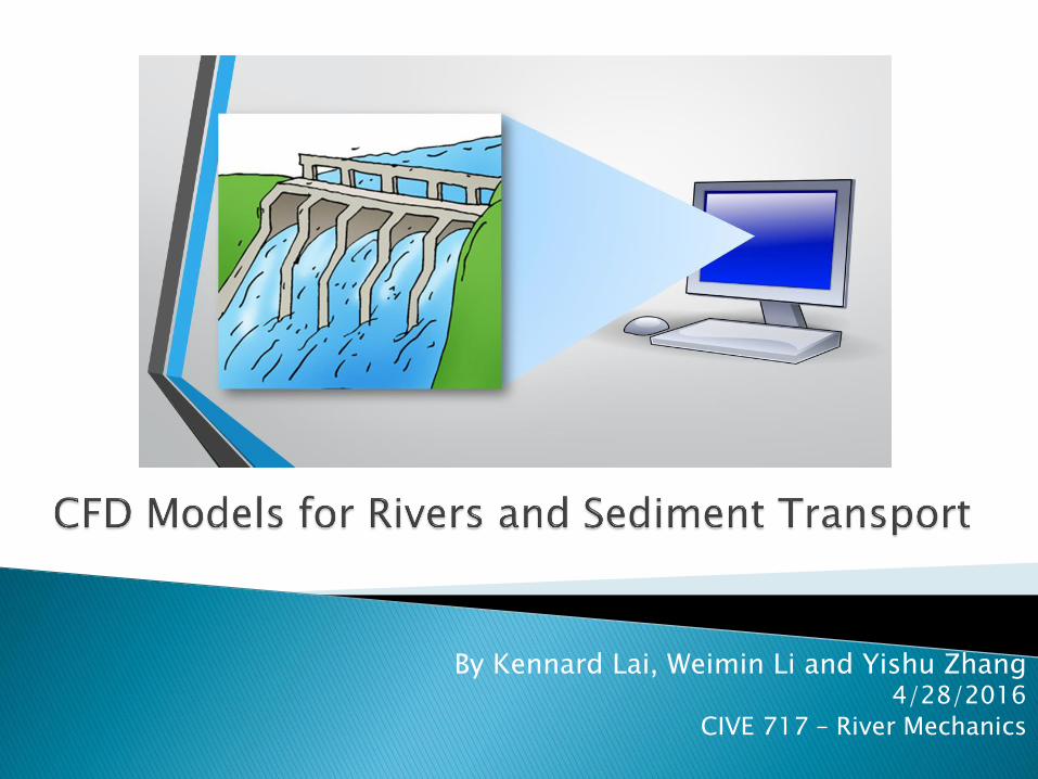
• Sediment transport in rivers
• Sediment deposition in reservoirs
• Waves driven by wind shear on reservoir
• Detention time of chlorine in baffle tanks in water
treatment facilities
• Modeling pollution flumes from off-shore fish farms
• Design of whitewater kayak parks
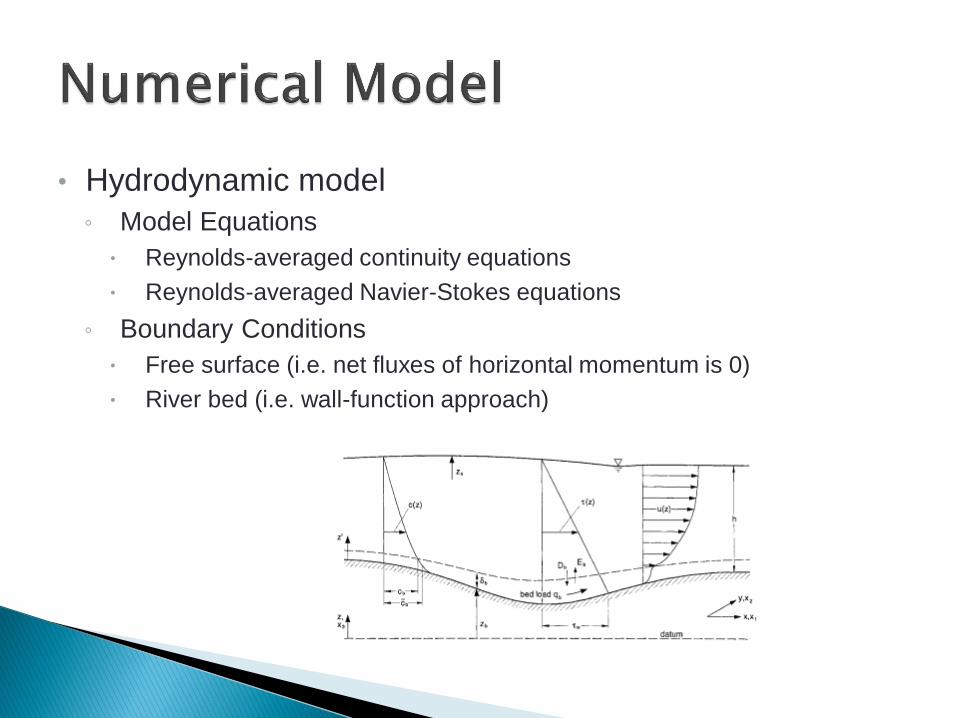
• Hydrodynamic model
◦ Model Equations
Reynolds-averaged continuity equations
Reynolds-averaged Navier-Stokes equations
◦ Boundary Conditions
Free surface (i.e. net fluxes of horizontal momentum is 0)
River bed (i.e. wall-function approach)
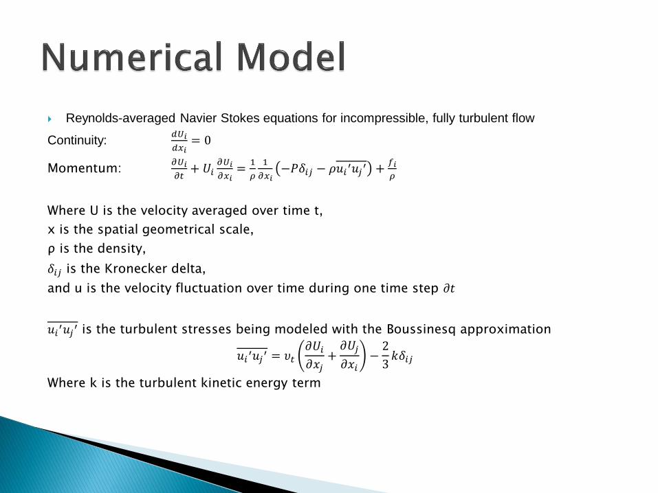
Reynolds-averaged Navier Stokes equations for incompressible, fully turbulent flow
Continuity: 𝑑𝑈𝑖
𝑑𝑥𝑖= 0
Momentum: 𝜕𝑈𝑖
𝜕𝑡+ 𝑈𝑖
𝜕𝑈𝑖
𝜕𝑥𝑖=
1
𝜌
1
𝜕𝑥𝑖−𝑃𝛿𝑖𝑗 − 𝜌𝑢𝑖 ′𝑢𝑗′ +
𝑓𝑖
𝜌
Where U is the velocity averaged over time t,
x is the spatial geometrical scale,
ρ is the density,
𝛿𝑖𝑗 is the Kronecker delta,
and u is the velocity fluctuation over time during one time step 𝜕𝑡
𝑢𝑖′𝑢𝑗′ is the turbulent stresses being modeled with the Boussinesq approximation
𝑢𝑖′𝑢𝑗
′ = 𝜐𝑡𝜕𝑈𝑖𝜕𝑥𝑗
+𝜕𝑈𝑗
𝜕𝑥𝑖−2
3𝑘𝛿𝑖𝑗
Where k is the turbulent kinetic energy term

• Sediment transport model
◦ Bed load transport
Sediment mass-balance equation
◦ Suspended load transport
Convection-diffusion equation
◦ Empirical Input
Near bed equilibrium concentration at a reference level
Equilibrium bed load transport
Non-equilibrium adaptation length

• The governing equations are approximated over control
volumes or a grid
• 1-D Grid
◦ Water surface elevation model in hydraulics
(standard step method)
• 2-D Grid
◦ Cartesian, structured, and unstructured
• 3-D Grid
◦ Three dimensional grids are very computationally expensive
◦ Grid sizes are smaller in areas with high gradients to capture the
range of motions and boost accuracy and efficiency
• Unstructured grids (most common)
• Coarse grid causes instabilities close to the boundary
◦ Inflation
◦ Changing shapes

• Physical experiments must always be used to validate
CFD codes
• Good agreement between model results and experiment
results indicates the CFD code is accurate and correct.

• Errors of O(∆x) in discretization of equations
• Errors caused by using averaged parameters (Reynolds averaged Navier-Stokes)
• Numerical physics
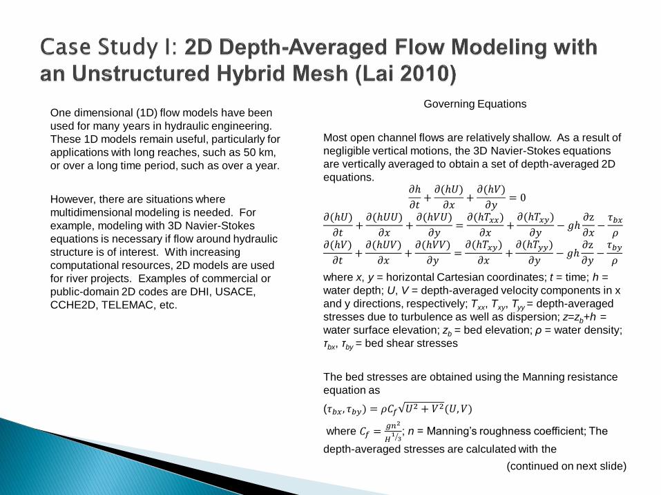
One dimensional (1D) flow models have been
used for many years in hydraulic engineering.
These 1D models remain useful, particularly for
applications with long reaches, such as 50 km,
or over a long time period, such as over a year.
However, there are situations where
multidimensional modeling is needed. For
example, modeling with 3D Navier-Stokes
equations is necessary if flow around hydraulic
structure is of interest. With increasing
computational resources, 2D models are used
for river projects. Examples of commercial or
public-domain 2D codes are DHI, USACE,
CCHE2D, TELEMAC, etc.
Governing Equations
Most open channel flows are relatively shallow. As a result of
negligible vertical motions, the 3D Navier-Stokes equations
are vertically averaged to obtain a set of depth-averaged 2D
equations. 𝜕ℎ
𝜕𝑡+𝜕(ℎ𝑈)
𝜕𝑥+𝜕(ℎ𝑉)
𝜕𝑦= 0
𝜕(ℎ𝑈)
𝜕𝑡+𝜕(ℎ𝑈𝑈)
𝜕𝑥+𝜕(ℎ𝑉𝑈)
𝜕𝑦=𝜕(ℎ𝑇𝑥𝑥)
𝜕𝑥+𝜕(ℎ𝑇𝑥𝑦)
𝜕𝑦− 𝑔ℎ
𝜕z
𝜕𝑥−𝜏𝑏𝑥𝜌
𝜕(ℎ𝑉)
𝜕𝑡+𝜕(ℎ𝑈𝑉)
𝜕𝑥+𝜕(ℎ𝑉𝑉)
𝜕𝑦=𝜕(ℎ𝑇𝑥𝑦)
𝜕𝑥+𝜕(ℎ𝑇𝑦𝑦)
𝜕𝑦− 𝑔ℎ
𝜕z
𝜕𝑦−𝜏𝑏𝑦𝜌
where x, y = horizontal Cartesian coordinates; t = time; h =
water depth; U, V = depth-averaged velocity components in x
and y directions, respectively; Txx, Txy, Tyy = depth-averaged
stresses due to turbulence as well as dispersion; z=zb+h =
water surface elevation; zb = bed elevation; ρ = water density;
τbx, τby = bed shear stresses
The bed stresses are obtained using the Manning resistance
equation as
(𝜏𝑏𝑥 , 𝜏𝑏𝑦) = 𝜌𝐶𝑓 𝑈2 + 𝑉2(𝑈, 𝑉)
where 𝐶𝑓 =𝑔𝑛2
𝐻13 ; n = Manning’s roughness coefficient; The
depth-averaged stresses are calculated with the
(continued on next slide)

Boussinesq’s formulation as 𝑇𝑥𝑥 = 2(𝜗 + 𝜗𝑡)𝜕𝑈
𝜕𝑥,
𝑇𝑦𝑦 = 2(𝜗 + 𝜗𝑡)𝜕𝑉
𝜕𝑦, 𝑇𝑥𝑦 = 2(𝜗 + 𝜗𝑡)(
𝜕𝑈
𝜕𝑦+
𝜕𝑉
𝜕𝑥) where
ν = kinematic viscosity of water, and νt = eddy
viscosity
The eddy viscosity is calculated with a turbulent
model. Dr. Lai has used two models in his study,
the depth-averaged parabolic model and the two-
equation k-ε model. For the parabolic model, the
eddy viscosity is calculated as
𝜗𝑡 = 𝐶𝑡𝑈∗ℎ
where Ct = the model constant with the range from
0.3 to 1.0. A default value of 0.7 is used in Dr. Lai’s
study; 𝑈∗ = 𝐶𝑓1 2 𝑈2 + 𝑉2
For the two-equation k-ε model, the eddy viscosity is calculated
as 𝜗𝑡 = 𝐶𝜇𝑘2/휀 with the two additional equations as following.
𝜕(ℎ𝑘)
𝜕𝑡+𝜕(ℎ𝑈𝑘)
𝜕𝑥+𝜕(ℎ𝑉𝑘)
𝜕𝑦
=𝜕
𝜕𝑥
ℎ𝜗𝑡𝜎𝑘
𝜕𝑘
𝜕𝑥+
𝜕
𝜕𝑦
ℎ𝜗𝑡𝜎𝑘
𝜕𝑘
𝜕𝑦+ 𝑃ℎ + 𝑃𝑘𝑏 − ℎ𝜖
𝜕(ℎ𝜖)
𝜕𝑡+𝜕(ℎ𝑈𝜖)
𝜕𝑥+𝜕(ℎ𝑉𝜖)
𝜕𝑦
=𝜕
𝜕𝑥
ℎ𝜗𝑡𝜎𝜖
𝜕𝜖
𝜕𝑥+
𝜕
𝜕𝑦
ℎ𝜗𝑡𝜎𝜖
𝜕𝜖
𝜕𝑦+ 𝐶𝜖1
𝜖
𝑘𝑃ℎ + 𝑃𝜖𝑏
− 𝐶𝜖2ℎ𝜖2
𝑘
Following Rodi’s recommendation, one has
𝑃ℎ = ℎ𝜗𝑡[2(𝜕𝑈
𝜕𝑥)2+2(
𝜕𝑉
𝜕𝑦)2 + (
𝜕𝑈
𝜕𝑦+
𝜕𝑉
𝜕𝑥)2], 𝑃𝑘𝑏 = 𝐶𝑓
−1 2 𝑈∗3,
𝑃𝜖𝑏 = 𝐶𝜖Γ𝐶𝜖2𝐶𝜇−1 2 𝐶𝑓
−3 4 𝑈∗4ℎ, 𝐶𝜇 = 0.09, 𝐶𝜖1 = 1.44, 𝐶𝜖2 = 1.92,
𝜎𝑘 = 1,
𝜎𝜖 = 1.3, 𝐶𝜖Γ = 1.8 − 3.6
Boundary Conditions
Boundary conditions consist of four types: inlet, exit, solid wall, and symmetry.
(1)Inlet: A total flow discharge, in the form of a constant or a time series hydrograph, is specified. Velocity distribution along the inlet is calculated in a way that the total discharge is satisfied. If a flow is subcritical at an inlet, however, the water surface elevation is not needed; instead a constant water surface slope normal to the inlet is assumed. If a flow is supercritical at the inlet, however, the water surface elevation at the inlet is needed as another input. If the k-ε model is used, the values of k and ε are also needed which, for most applications, have negligible impact on the flow pattern.
(2)Exit: Water surface elevation is specified at a subcritical exit but it is not required if flow at the exit is supercritical. Instead, it is assumed that the derivative of the water surface elevation normal to the exit is constant at the supercritical exit.
(3)Solid wall: no-slip condition is applied and the wall functions are employed. At a solid wall,
(𝜏𝑏𝑥 , 𝜏𝑏𝑦) = 𝜌𝐶𝜇1 4 𝑘𝑝
1 2 𝑘(𝑈, 𝑉) ln(𝐸𝑦𝑝+) where 𝑦𝑝
+ = 𝐶𝜇1 4 𝑘𝑝
1 2 𝑦𝑝 𝜗 for the k-ε model and 𝑘𝑝=turbulent kinetic energy at a mesh
cell that contains the wall boundary; and (𝜏𝑏𝑥 , 𝜏𝑏𝑦) = 𝜌𝑈∗𝑘(𝑈, 𝑉) ln(𝐸𝑦𝑝+) where 𝑦𝑝
+ = 𝑈∗𝑦𝑝 𝜗 for the depth-averaged
parabolic model where 𝑘 = vonKarmanconstant, 0.41, 𝑦𝑝 = normal distance from the center of a cell to a wall, and E = constant, 9.758.
(4)Symmetry: The normal velocity component is set to zero at a symmetry boundary.
Discretization
The 2D depth-averaged may be written in tensor form as
where V = velocity vector, T = second-order stress tensor, τb = bed shear stress
vector
As an illustration, consider a generic convection-diffusion equation that is
representative of all governing equations
where Φ = a dependent variable, a scalar or a component of a vector,
Γ = diffusivity coefficient, S*Φ = source/sing term
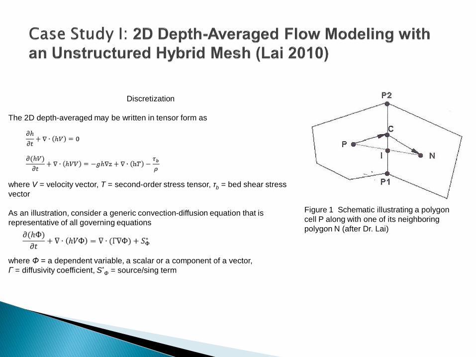
Figure 1 Schematic illustrating a polygon
cell P along with one of its neighboring
polygon N (after Dr. Lai)
Integration over an arbitrarily shaped polygon P shown in
the Figure 1 leads to
(ℎ𝑝𝑛+1𝛷𝑝
𝑛+1 − ℎ𝑝𝑛𝛷𝑝
𝑛)𝐴
∆𝑡+ (ℎ𝑐𝑉𝑐|𝑠|)
𝑛+1𝛷𝐶𝑛+1
𝑎𝑙𝑙𝑠𝑖𝑑𝑒𝑠
= (𝛤𝑐𝑛+1𝛻𝛷𝑛+1 ∙ 𝑛|𝑠|)
𝑎𝑙𝑙𝑠𝑖𝑑𝑒𝑠
+ 𝑆𝛷
where Δt = time step, A = cell area, Vc = Vc·n = velocity
component normal to the polygonal side (e.g. P1P2 in the
figure 1) and is evaluated at the side center C, n = unit
normal vector of a polygon side, s = polygon side
distance vector, and SΦ = S*ΦA, subscript C indicates a
value evaluated at the center of a polygon side and
superscripts n or n+1 denotes the time level.
𝛻𝛷 ∙ 𝑛 𝑠 = 𝐷𝑛 𝛷𝑁 − 𝛷𝑃 +𝐷𝑐 𝛷𝑃2 − 𝛷𝑃1
𝐷𝑛 =𝑠
(𝑟1 + 𝑟2) ∙ 𝑛
𝐷𝑐 =(𝑟1 + 𝑟2) ∙ 𝑠 |𝑠|
(𝑟1 + 𝑟2) ∙ 𝑛
The implicit solver requires the solution of nonsymmetric sparse
matrix linear equations. In Dr. Lai’s study, the standard
conjugate gradient solver with ILU preconditioning is used.
Wetting and Drying Treatment
Most natural rivers consist of main and side channels, bars,
inlands, and floodplains and the bed may be wet or dry
depending on flow stage. The wetting-drying property is not
known and is part of the solution. A robust wetting-drying
algorithm, therefore, is needed. Such an algorithm offers the
benefit that the same solution domain and mesh may be used
for all flow discharges. A cell is wet if water depth is above 1.0
mm.

Sandy River Delta Simulation
The SANDY River Delta dam is located near the
confluence of the Sandy and Columbia rivers, east of
Portland, Oregon (Figure 2). As a result of its closure
in 1938, flow has been redirected from the east
distributary to the west (downstream) distributary.
Although it was once the main distributary channel, the
east distributary is currently only activated under high
flow conditions. New efforts to improve aquatic habitat
conditions have considered the removal of the dam.
This model was used to evaluate possible effects on
the delta area if the dam is removed. The bed
elevation contours of the study area are displayed in
the Figure 2.
Figure 2 Study area of the Sandy and Columbia River confluence,
along with the topography for the solution domain (after Dr. Lai)
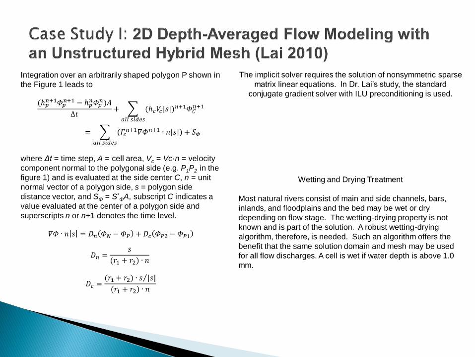
The solution domain was covered with a hybrid mesh with a total of 37,637 cells, A portion of the mesh around the
delta is shown in the Figure 3.
Figure 3 Portion of the mesh used to model the Sandy River and Columbia River Delta (after Dr. Lai)

Flow resistance is a model input represented by the Manning’s coefficient n. The solution domain was divided into a number of roughness zones based on the underlying bed properties, delineated using the available aerial photo and the bed gradation data. In the figure 14, the zones 1, 2, and 3 represent the main channel of the Sandy River; zones 4 and 5 represent the main channel of Columbia River; Zone 6 consists mostly of sand bars and less vegetated areas; and zone 7 represents islands and floodplains with heavy vegetation. The calibrated Manning’s coefficients are tabulated in the Table 1.
Figure 4 Roughness zones used for the Sandy River Delta (after Dr. Lai)
Table 1 Manning’s coefficient for Different Zones shown in the Figure 4
Zone number 1 2 3 4 5 6 7
Manning’s n 0.035 0.06 0.15 0.035 0.035 0.035 0.06
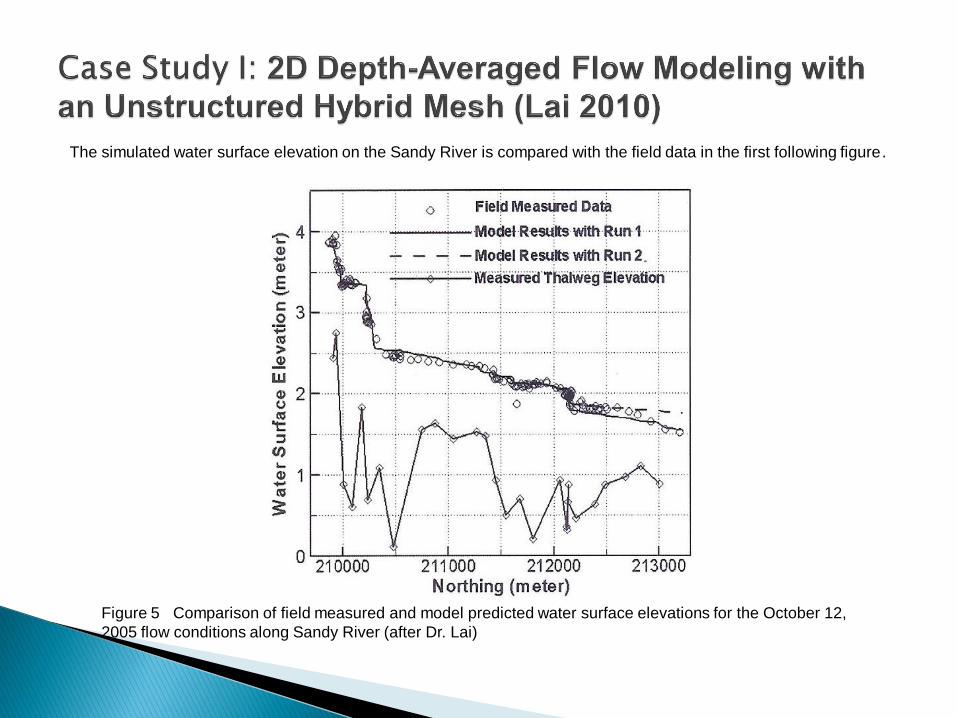
The simulated water surface elevation on the Sandy River is compared with the field data in the first following figure.
Figure 5 Comparison of field measured and model predicted water surface elevations for the October 12,
2005 flow conditions along Sandy River (after Dr. Lai)

The measured and predicted velocity magnitude
comparisons at all measurement points are
made for both the Sandy River and Columbia
River. The comparison of Sandy River is shown
below. The agreement between the model and
measured data are reasonable.
Figure 6 Comparison of field measured and model
predicted depth-averaged velocity for the October 12,
2005 flow conditions along the Sandy River (after Dr. Lai)
Conclusion
Dr. Lai’s numerical method is well suited
to natural river flows with a combination
of main channels, side channels, bars,
floodplains, and in-stream structures.

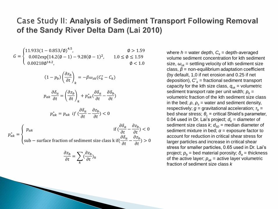
Sediment Transport Equations
The sediment is assumed to be non-cohesive and non-uniform and is divided into a number of sediment size classes. One
has non-equilibrium sediment transport equation for each size class k below.
𝜕(ℎ𝐶𝑘)
𝜕𝑡+𝜕(ℎ𝑈𝐶𝑘)
𝜕𝑥+𝜕(ℎ𝑉𝐶𝑘)
𝜕𝑦= 𝛽𝜔𝑠𝑘(𝐶𝑘
∗ − 𝐶𝑘)
𝐶𝑘∗ = 𝑞𝑠𝑘 𝑞
𝑞𝑠𝑘𝑔(𝑠 − 1)
(𝜏𝑏 𝜌 )1.5= 𝑝𝑘𝐺(∅𝑘)
𝑠 =𝜌𝑠𝜌
Shield’s parameter of sediment size class k
𝜃𝑘 =𝜏𝑏
𝜌𝑔(𝑠 − 1)𝑑𝑘
∅𝑘 =𝜃𝑘𝜃𝑐(𝑑𝑘𝑑50
)𝛼
𝐺 = 11.933(1− 0.853 ∅) 4.5
, ∅ > 1.59
0.002exp[14.2 ∅ − 1 − 9.28 ∅ − 1 2, 1.0 ≤ ∅ ≤ 1.59
0.00218∅14.2, ∅ < 1.0
1 − 𝑝𝑏𝜕𝑧𝑏𝜕𝑡
𝑘
= −𝛽𝜔𝑠𝑘(𝐶𝑘∗ − 𝐶𝑘)
𝑝𝑎𝑘𝜕𝛿𝑎𝜕𝑡
=𝜕𝑧𝑏𝜕𝑡
𝑘
+ 𝑝𝑎𝑘∗ (
𝜕𝛿𝑎𝜕𝑡
−𝜕𝛿𝑏𝜕𝑡
)
𝑝𝑎𝑘∗ = 𝑝𝑎𝑘𝑖𝑓(
𝜕𝛿𝑎𝜕𝑡
−𝜕𝑧𝑏𝜕𝑡
) < 0
𝑝𝑎𝑘∗ =
𝑝𝑎𝑘 if(𝜕𝛿𝑎𝜕𝑡
−𝜕𝑧𝑏𝜕𝑡
) < 0
sub − surfacefractionofsedimentsizeclasskif(𝜕𝛿𝑎𝜕𝑡
−𝜕𝑧𝑏𝜕𝑡
) > 0
𝜕𝑧𝑏𝜕𝑡
= (𝜕𝑧𝑏𝜕𝑡
)𝑘𝑘
where h = water depth, Ck = depth-averaged
volume sediment concentration for kth sediment
size, ωsk = settling velocity of kth sediment size
class, β = non-equilibrium adaptation coefficient
(by default, 1,0 if net erosion and 0.25 if net
deposition), C*k = fractional sediment transport
capacity for the kth size class, qsk = volumetric
sediment transport rate per unit width; pk =
volumetric fraction of the kth sediment size class
in the bed; ρ, ρs = water and sediment density,
respectively; g = gravitational acceleration; τb =
bed shear stress; θc = critical Shield’s parameter,
0.04 used in Dr. Lai’s project; dk = diameter of
sediment size class k; d50 = median diameter of
sediment mixture in bed; α = exposure factor to
account for reduction in critical shear stress for
larger particles and increase in critical shear
stress for smaller particles, 0.65 used in Dr. Lai’s
project; pb = bed material porosity; δa = thickness
of the active layer; pak = active layer volumetric
fraction of sediment size class k
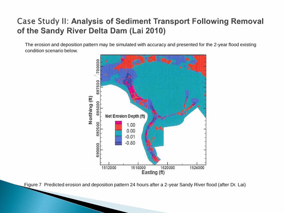
The erosion and deposition pattern may be simulated with accuracy and presented for the 2-year flood existing
condition scenario below.
Figure 7 Predicted erosion and deposition pattern 24 hours after a 2-year Sandy River flood (after Dr. Lai)

Bed changes in a section of the
Danube river for before and after
the flood of 2002
Purpose: To investigate the
possibility of modeling the bed-
changes in a natural river using a
3-D numerical model for
prediction of effects of floods or
alterations of the physical
characteristics of the river
Measured water depths before (b) and after (c) the flood. Measured (d) and computed (e) elevation changes. (a) identifies special regions further discussed in the paper

Model type: Full 3D CFD model
Equations:
Navier Stokes Equations using the k-
epsilon turbulence closure
Nonuniform sediment rating curve from
Wu et al. (2000)
Width-to-depth ratio: 60
Depth-to-grain size ratio: 200
Mean grain size, dm = 26 mm
Groynes and vegetated areas (green)
Median grain size, d50 at the end of the computation

Calculated bed changes, reference calculations with Strickler bed roughness:
(a) ks=0.12 m
(b) ks=0.2 m
(c) ks=0.075 m
(d) ks=2d50
(e) ks=4d50
Parameter Sensitivity Analysis:
• Varying grid resolution
• Varying time step
• Varying sediment transport
parameters
Conclusions:
“CFD model performed well when
compared with field measurements.
Model was able to represent
morphodynamic process, such as
deposition processes of a bar and
related erosion processes at the
scour on the opposite side”

Environmental concerns led to increase run-of-river intakes for
hydroelectric projects, replacing conventional deep reservoir intakes.
Run-of-river intakes have higher approach flow velocities and
turbulence, leading to increased sediment inflow at intake.
Purpose: ◦ Utilize CFD to evaluate potential construction cost savings by reducing excavation
downstream from the powerhouse and spillway and potential impact on flow hydraulics.
◦ Analyze different intake layouts to minimize head losses and provide more uniform
velocity distribution at the intake
◦ Assess potential of sediment into intake

Powerhouse intake layout design
Flow conditions are highly non-uniform
Large eddy in the approach channel contributed to head losses
Spur dyke caused uneven flow distribution
Optimized layout: ◦ Flow of intake moved farther upstream, curved guiding walls,
spur dyke removed, lowered invert elevation along the right size of the approach channel entrance

Hydraulics of sediment training wall
Usually a training wall is parallel to approach flow direction to increase flushing efficiency. But in this case the the approach flow is almost parallel to the dam, attacking the training wall at at acute angle
CFD showed that the training wall caused very turbulent flow conditions with increased local velocities
As a result, no training wall was included in the design
With the advance of computing technology, numerical simulations using CFD is proven to be useful tool in hydraulic engineering
CFD is viable, and more cost-effective complement, if-not-alternative to physical modeling

Fischer-Antze, T., N.R.B. Olsen, and D. Gutknecht (2008), Three-dimensional CFD modeling of morphological bed changes in the Danube River, Water Resources Research 44, W09422, DOI: 10.1029/2007WR006402
Jose Vasquez, Hurtig, K., Hughes, B., (accessed on 2016), Computational Fluid Dynamics (CFD) Modeling of Run-of-River Intakes, Northwest Hydraulic Consultatns Ltd., North Vancouver, Canada
Weiming Wu, Sam S.Y. Wang, Tafei Jia (2000) Nonuniform sediment transport in alluvial rivers, Journal of Hydraulic Research, 38:6, 427-434, DOI: 10.1080/00221680009498296
Yong G. Lai, 2010, 2D Depth-Averaged Flow Modeling with an Unstructured Hybrid Mesh, Journal of Hydraulic Engineering, 136(1), pp 12-23
Yong G. Lai. 2006, Analysis of Sediment Transport Following Removal of the Sandy River Delta Dam, US Bureau of Reclamation