BY - COREincompressible and compressible flows. It is believed that Reynolds stress models would...
183
NUMERICAL SIMULATION OF INCOMPRESSIBLE AND COMPRESSIBLE FLOW BY ZHIYIN YANG THESIS SUBMITTED TO THE UNIVERSITY OF SHEFFIELD FOR THE DEGREE OF DOCTOR OF PHILOSOPHY DEPARTMENT OF MECHANICAL AND PROCESS ENGINEERING UNIVERSITY OF SHEFFIELD FEBRUARY, 1989
Transcript of BY - COREincompressible and compressible flows. It is believed that Reynolds stress models would...

NUMERICAL SIMULATION OF
INCOMPRESSIBLE AND COMPRESSIBLE FLOW
BY
ZHIYIN YANG
THESIS SUBMITTED TO THE
UNIVERSITY OF SHEFFIELD FOR THE DEGREE OF
DOCTOR OF PHILOSOPHY
DEPARTMENT OF MECHANICAL AND PROCESS ENGINEERING
UNIVERSITY OF SHEFFIELD
FEBRUARY, 1989
SUMMARY
This thesis describes the development of a numerical solution procedure which
is valid for both incompressible flow and compressible flow at any Mach number.
Most of the available numerical methods are for incompressible flow or compress-
ible flow only and density is usually chosen as a main dependent variable by
almost all the methods developed for compressible flow. This practice limits the
range of the applicability of these methods since density changes can be very
small when Mach number is low. Even for high Mach number flows the exist-
ing time-dependent methods may be inefficient and costly when only the finial
steady-state is of concern. The presently developed numerical solution proce-
dure, which is based on the SIMPLE algorithm, solves the steady-state form of
the Navier-stokes equations, and pressure is chosen as a main dependent variable
since the pressure changes are always relatively larger than the density changes.
This choice makes it possible that the same set of variables can be used for both
incompressible and compressible flows.
It is believed that Reynolds stress models would give better performance in
some cases such as recirculating flow, highly swirling flow and so on where the
widely used two equation k-e model performs poorly. Hence, a comparative study
of a Reynolds stress model and the k-e model has been undertaken to assess their
performance in the case of highly swirling flows in vortex throttles. At the same
time the relative performance of different wall treatments is also presented.
It is generally accepted that no boundary conditions should be specified at
the outflow boundary when the outflow is supersonic, and all the variables can
11

be obtained by extrapolation. However, it has been found that this established
principle on the outflow boundary conditions is misleading, and at least one
variable should be specified at the outflow boundary. It is also shown that the
central differencing scheme should be used for the pressure gradient no matter
whether it is subsonic or supersonic flow.
iii

ACKNOWLEDGEMENTS
I would like to express my sincere thanks to Prof. J. Swithenbank for his
supervision, encouragement and many helpful suggestions during the study.
I am also grateful to many academic and technical staff, and to my colleagues
in the department for their advice and assistance, especially to Dr. F. Boysan
who gave me great help at the initial stage of the work.
The author is also indebeted to the Chinese Government and the British
Council for their financial sponsorship.
iv

Contents
SUMMARY ii
ACKNOMLEDGEMENTS iv
CONTENTS V
NOMENCLATURE X
1 INTRODUCTION 1
1.1 Numerical Flow Simulations .... .... .... ... .... .. 1
1.2 Incompressible Flows ... ..... .... ..... ..... . .. 3
1.3 Compressible Flows .......................... 5
1.4 Turbulence ....... ......... ............... 6
1.5, The Objectives of The Present Study . ....... .... .... 8
1.6 Outline of The Thesis .......................... 9
2 LITERATURE SURVEY 11
2.1 Methods for Incompressible Flows .......... ........ 11
2.1.1 The Poisson Equation Method ................ 12
V
2.1.2 Artificial Compressibility Method . ..... ...... .. 13
2.1.3 Pressure Correction Methods ... ......... .... 14
2.2 Methods for Compressible Flows ........... ........ 18
2.2.1 Unsteady Methods ...................... 19
2.2.2 Steady Methods ..... .... .... ....... .... 24
3 GOVERNING EQUATIONS AND TURBULENCE MODELLING
30
3.1 Basic Equations .... ........................ 31
3.1.1 Continuity Equation .... ......... ........ 31
3.1.2 Momentum Equations . ...... .... ..... .... 31
3.1.3 Energy Equation . ... .... .... . .... .... .. 33
3.1.4 Equation of State .... .... .......... ..... 34
3.2 Time-Averaging Procedure ... .... ......... .... .. 35
3.3 Turbulence Modelling .............. ... ...... .. 36
3.3.1 Zero Equation Models . .... .... ..... ...... 39
3.3.2 One Equation Models .... .... ....... ...... 40
3.3.3 Two Equation Models . .... .... ... .... .... 42
3.3.4 Stress Equation Models ....... ..... ...... .. 45
3.3.5 Multiple-Scale Models .................... 55
3.3.6 Other Approachs to Turbulence Modelling ..... .... 57
4 SOLUTION PROCEDURE 59
4.1 The Finite Difference Equations ...... ........... .. 60
vi

4.2 Solution of the Difference Equations .... ..... .... .... 61
4.3 Boundary Conditions . ....... ..... . ..... ...... 62
4.4 Treatment of Velocity-Pressure Coupling . ..... ........ 63
4.4.1 The SIMPLE Algorithm ................... 64
4.4.2 Modifications for Subsonic Flow ........... .... 67
4.4.3 Modifications for Supersonic Flow ... ... .... .... 69
4.4.4 The Pressure-Correction Equation ... .... ....... 73
4.4.5 Summary of the Solution Procedure ......... .... 77
5 APPLICATIONS TO STRONGLY SWIRLING FLOWS 79
5.1 Introduction .... .... ..... .... ..... .... .... 80
5.2 Governing Equations . ..... ........ ....... .... 83
5.2.1 The Reynolds stress model .................. 83
5.2.2 The k-c Model ......................... 85
5.3 Wall Treatment .... ..... ...... ..... ........ 87
5.3.1 The Conventional Wall Treatment . ............. 87
5.3.2 The Modified Wall Treatment ................ 89
5.4 Boundary Conditions . ......... .... ....... .... 91
5.4.1 Inlet Boundary ..... .... .... ..... ...... 91
5.4.2 Outlet Boundary ....................... 91
5.4.3 Wall Boundary and Symmetry Line ....... ... . .. 92
5.5 Geometry of Vortex Throttles .................... 92
5.6 Results and Comparisons ...... . ... ....... .... .. 93
VII

5.7 Discussions of the Results ... .... ....... ...... .. 96
5.7.1 Pressure Field . ..... .... ....... .... .... 97
5.7.2 Flow Field ........................... 98
5.7.3 The Effects of Reynolds Number . ....... ...... 99
5.7.4 Effect of Inlet Swirl Intensity ..... ........... 100
5.7.5 Effect of Inlet Turbulent Intensity .............. 101
5.7.6 Pressure Drop . ..... .... ........... .... 101
5.8 Conclusions .... .... ......... ............. 104
6 APPLICATIONS TO COMPRESSIBLE FLOWS 119
6.1 Governing Equations .......... ............... 120
6.2 Convergent and Divergent Nozzle Flows ...... .... .... 120
6.2.1 Analytical Solution ....... .... ........... 121
6.2.2 Numerical Solution ... .... ....... .... .... 122
6.2.3 Results and Comparison ................... 126
6.3 Channel Flow . .... ..... .... .... ....... .... 129
6.3.1 Geometry of the Channel ................... 129
6.3.2 Boundary Conditions .... ........ . .... .... 130
6.3.3 Results and Comparison .... ....... ........ 130
6.4 Flow Behind a Rearward-Facing Step . .... ..... ...... 133
6.4.1 Flow Geometry ..... .... .... ........... 133
6.4.2 Boundary Conditions ........ ............. 134
6.4.3 Results and Comparison ................... 134
vi"
6.5 Closure ... .... ....... ........ ... .... .... 135
7 CLOSURE 148
7.1 A Review of The Thesis . ... .... .... ... ...... .. 148
7.1.1 Turbulence Models .............. .... .... 149
7.1.2 Numerical Aspects ....... ......... ...... 151
7.1.3 Validation of the Prediction Procedure ..... .... .. 152
7.1.4 Applications to Other Cases ...... ....... .... 153
7.2 Suggestions for Future Work ...... ......... ..... . 154
REFERENCES 157
ix

NOMENCLATURE
ap, aw, aE, a N, as Coefficients in the discretization equations
a Local sound velocity
Ap, Ayi., AE, AN, As Area of cell boundaries
A Cross section area of nozzles
A* Throat area of nozzles
C1, C2, CD , Ca, Ce,
CT, Cµ, CEI, CE2 Turbulence model constants
C1 X/Cµ4
Cp Specific heat at constant pressure
C. Specific heat at constant Volume
DU p
Ap/ap
D; j Diffusion tensor
e Internal energy
E, E**, b, s, m Constants and parameters used in wall functions
f Body force
g Heat transfer by conduction
h Enthalpy
K 1/RT
k Turbulent kinetic energy
k Thermal conductivity
I Mixing length
M Mach number
X

p Fluctuating pressure
P Mean pressure
P* Stagnation pressure
P Production term in the k-equation
Pe Peclet number
P; j Production tensor
Pr Prandtl number
Prk Prandtl number for turbulent kinetic energy
Pr, Prandtl number for dissipation rate
Q Heat generation
r Radial ,tct ut ýº, t,
R Gas constant
Re Reynolds number
R; j Reynolds stress tensor
S Source term
t Time
T Temperature
T* Stagnation temperature
pu; ui Reynolds stress tensor
u, v, w Fluctuating velocities
U, V, W Mean velocities
x, y, z Cartesian coordinates
Vt characteristic velocity of turbulence
xi

GreekSymbols
a The Reynolds stress model constant
p Density
P Stagnation density
T Shear stress
Tw Wall shear stress
T{j Viscous stress tensor
v Kinematic viscosity
IZ Viscosity
fttu,. Turbulent Viscosity
lief f Effective Viscosity, ptu,. +µ
rc Von Karman constant
li* f, 114 µ
Dissipation function
4) ij Pressure-strain tensor
y Ratio of specific heats
r CTk2/E
r, Ck2/E Kronecker delta function
Turbulent kinetic energy dissipation rate
w Time-averaged square of the vorticity fluctuation
Subscripts
e Denotes edge of inertial sub-layer
X11
nb Denotes neighbouring points
P Central point of control volume
v Denotes edge of viscous sub-layer
W, E, N, S Neighbouring points
w, e, n, s Neighbouring points at control volume boundaries
Superscripts
U Related to axial direction
V Related to radial direction
- Averaged value
' Fluctuating value, or correction value
* Intermediate value, or stagnation value
X111

Chapter 1
INTRODUCTION
1.1 Numerical Flow Simulations
In the last decade, advances in computer technology and data communication
have speeded up numerical flow simulations enormously. The availability of
modern supercomputers and the ingenuity of computational fluid dynamics re-
searchers have resulted in new methods for solving historically intractable non-
linear flow field problems. Advances in data communication have facilitated
remote access to those computing engines, and advances in computer technology
incorporated in mini- and midicomputers now provide sophisticated interactive
graphics and data manipulation capability. All of these have brought about pro-
found effects on the engineering design process (1).
It is generally accepted that fluid dynamics can be divided into theoretical,
experimental and computational branches (2). Analytical methods provide quick,
closed-form solutions, but they require unduly restrictive assumptions, can handle
1

only very simple configurations, and capture only the idealized fluid dynamics.
Through experimentation, representative or actual configurations can be tested
and representative or completely experimental data can be obtained. However,
experimentation is costly both in terms of model and actual test time. In addi-
tion, the limited conditions that can be attained by experimental facilities restrict
the scope of experimental programs. By comparison, computational procedures
require few restrictive assumptions and can be used to treat complicated configu-
rations. Moreover, they have few Mach number or Reynolds number limitations,
they have complete control over fluid properties such as density, viscosity etc.,
they have enormous flexibility in the choice of flow parameters, in particular,
they can do what neither analytical methods nor experimental methods can do
- to test the sensitivity of phenomena to independent theoretical approximations
such as constant viscosity coefficient, neglect of buoyancy forces, unit Prandtl
number etc., and most important, they are far more cost effective than exper-
iments. Thus, the desirability of numerical flow simulations is enhanced when
one considers that the cost of experiments is continually increasing because of
model, labour, and energy overhead, whereas the cost of computer simulations is
continually decreasing as a result of improved numerical procedures and advances
in computer technology (3).
In spite of the advantages and the rapid development of numerical flow sim-
ulations, it is not expected that computational methods will completely replace
experimental testing in the foreseeable future. Their roles instead are comple-
mentary. The inadequacies in computational simulations are primarily associated
2
with poor resolution of physical phenomena, and this is the direct result of insuf-
ficient computer power. If one accepts the unsteady Navier-Stokes equations as
an adequate system to describe fluid flows, then physical phenomena of interest
could be accurately simulated with sufficient computer power. However, current
computer power is inadequate to permit numerical solution of these equations
with suitable resolution of the wide range of length scales active in high Reynolds
number turbulent flows. As a result of this, the averaged Navier-Stokes equations
have to be used at present. Computations require an adequate turbulence model
to correctly simulate viscous dominated flows (4).
It is such a comparative weighing of all the advantages and disadvantages
that underlies the growth of computational fluid dynamics and, especially, its
increasing role in design of new flight vehicles. Many numerical methods have
been developed but most of these methods are specific for either incompressible or
compressible flows; for either unsteady or steady flows. In the next two sections,
some general features of incompressible and compressible flows will be given,
which result in different numerical methods.
1.2 Incompressible Flows
The very obvious point is that density does not vary with the change of pres-
sure for incompressible flows. In other words, density is totally decoupled from
pressure and can be assumed constant. As a result, the time derivative term in
the continuity equation vanishes and density can be dropped from the continuity
3

equation. Therefore, neither density nor pressure can be directly associated with
the incompressible continuity equation. The continuity equation, in this case,
assumes only the role of a compatibility condition on the velocity field. This is
very important to the choice of the main dependent variables in the calculation
procedures.
It is apparent from what is mentioned above that density cannot be cho-
sen as a main dependent variable. Thus, there must be a way of calculating
pressure in order to solve the momentum equations. For two dimensional flows
the vorticity-stream function approach has been used very successfully instead
of solving the `primitive' equations. However, for three dimensional flows the
stream function as such does not exist, i. e., there is not a function such that its
isoline is the streamline. Nevertheless, a vorticity -stream function like system
has been formulated (2) to compute three dimensional incompressible flows in or-
der to avoid calculating pressure directly. Unfortunately, those methods require
more computer time and storage, and there may be some difficulties in specifying
boundary conditions.
The main obstacle arising from the choice of pressure as a main dependent
variable is that the original set of equations does not contain an equation for pres-
sure. Although a Poisson equation can be derived from the momentum equations
this method has not been widely used. An effective method to solve the `primi-
tive' equations had not been really developed until a mechanism was developed
by which the continuity and the momentum equations could be linked together to
produce a so called pressure correction equation for calculating pressure. It can
4

be said with confidence now that there is usually no difficulty in obtaining a good
numerical solution for incompressible flows. The current research in this field is
to refine the solution methods and to make them converge faster and perform
more effectively.
1.3 Compressible Flows
It is customary to calculate density directly from the continuity equation in the
case of compressible flows, and then pressure is obtained from the equation of
state. A great number of numerical methods with density as a main dependent
variable have been developed for unsteady flow problems and quite satisfactory
results have been obtained. But when only steady-state is concerned it usually
comes as a surprise to find that most (through not all) of the successful numerical
studies of steady-state flow problems are based on the time-dependent equations,
the steady-state solution being obtained, if it exists, as the asymptotic time
limit of the unsteady equations. The problem with density as a main dependent
variable is that pressure and density become weakly related and the variation of
density is almost negligible at low Mach numbers. Thus such an approach with
density as a main dependent variable is not viable. Even for supersonic flows in
some complicated configurations there exist some subsonic regimes where Mach
number can be very low. Furthermore, there are few methods developed for
solving the steady-state form of the compressible Navier-Stokes equations. It
is apparent that there is still considerable scope for further development and
5

improvements in this area.
1.4 Turbulence
Turbulence is one of the remaining unsolved problems in the area of physical
science. It is believed that the solution of the time-dependent three dimensional
Navier-Stokes equations and the conservation equations for mass and energy can
describe turbulent flows. However, the fastest and largest computers at present
are neither fast nor large enough to solve the equations directly for the required
range of length and time scale, even for simple flows. Many industrially im-
portant flows, such as the flow in a scramjet engine, are quite complex. The
basic problem in computations arises from the vast disparity in time and space
scales among the fundamental physical processes. Therefore, it is of practical im-
portance to describe turbulent flows in terms of time averaged quantities rather
than instantaneous. This kind of description leads to the well known turbulence
closure problem. The time-average processing of the Navier-Stokes equations
brings more unknowns, so called Reynolds stresses, which increase the number
of unknowns above the number of equations. The problem is then to supply the
information missing from the time-averaged equations by formulating a model to
describe some or all of the six independent Reynolds stresses.
Most turbulence models developed and tested so far are only for incompress-
ible flows. Some models give good predictions for certain flow configurations but
fail to give successful results in other cases (4). For flows with strong streamline
6
curvature such as highly swirling flows, it is expected that Reynolds stress models
which solve six partial differential equations for the six Reynolds stresses would
perform better. However, they have not been thoroughly tested for recirculat-
ing and swirling flows. Turbulence modelling is still a great challenge even for
incompressible flows.
The literature on turbulence modelling for compressible flows is much more
scarce. It is not expected that turbulence models developed for incompressible
flows can be applied successfully to compressible flows without any modifica-
tions. When the mass density is constant, as it is in all the turbulence models
for incompressible flows, all of the effects potentially depending on the vorticity
source term are absent. In chemically reactive flows the expansion due to heat
release influences turbulent mixing by providing the density gradient which leads
to vorticity generation (5). Even in non-reactive flows density gradients exist for
some cases. Furthermore, density fluctuations cannot be neglected when Mach
number is high. A successful turbulence model for compressible flows should in-
corporate the factors mentioned above. Unfortunately, such a model would be
very complicated and one has not been developed so far. Turbulence modelling
for compressible flows is still at an early stage, and many numerical simulations
for supersonic and hypersonic flows have been performed with very simple tur-
bulence models which contain many empirical factors. The big gap between the
"real world" and the models requires to be narrowed and a great deal of research
work in this area needs to be done.
7

1.5 The Objectives of The Present Study
The objectives of the present work are as follows:
1). Numerical methods for compressible flows have been highly developed
but they cannot be applied to low Mach number subsonic or incompressible flows
since density is used as a main dependent variable. Even for high Mach number
flows the existing time-dependent methods may not be very efficient when only
the final steady state is required. One of the main objectives of the present study
is to develop a prediction procedure which is valid for both incompressible and
compressible flows. The scheme, which is based on the SIMPLE (Semi-Implicit
Method for Pressure Linked Equations) method (6,7), solves the steady-state
form of the Navier-Stokes equations. Pressure is selected as a main dependent
variable since the pressure changes are always larger than the density changes
which become very small at low Mach numbers. This choice allows the same set
of variables to be used for both incompressible and compressible flows at any
Mach number.
2). Turbulence is still a remaining unsolved problem in the area of physics as
stated above. A number of turbulence models have been developed for incom-
pressible flows. Among those, the two equation k-e model (8) is the one most
widely used, and it provides an efficient way of calculating engineering flows.
But the performance of the standard k-e model becomes poor for some recircu-
lating flows, swirling flows and so on. It is believed that Reynolds stresses models
would give better performance but they have not well tested for some cases such
8
as highly swirling flows, One facet of the present work is to apply a Reynolds
stress model to the case of strongly swirling flows in vortex throttles and com-
pare the performance of the Reynolds stress model with that of the two equation
model. At the same time the relative performance of different wall treatments is
to be assessed.
1.6 Outline of The Thesis
In chapter two, a literature survey on numerical methods for both incompress-
ible and compressible flows is presented. As computational techniques have pro-
gressed dramatically and rapidly there are a great number of methods available.
Therefore, it is impossible to give a detailed survey within the scope of this thesis
since it is not the intention of the thesis to cover all aspects of numerical sim-
ulations of fluid flows. Bearing this in mind only the relevant finite-difference
methods for solving the `primitive' equations will be given in the survey.
In chapter three, the governing equations which describe the flows of a New-
tonian fluid are presented. The time-average processing which introduces more
unknowns is discussed. A general survey on turbulence models and some assump-
tions used in the process of modelling are presented.
Chapter four is devoted to the details of the prediction procedure. The cou-
pling between the continuity and the momentum equations together with the
discussion on the finite-difference scheme for the pressure gradient term in the
case of supersonic flows etc. are described.
9

In chapter five, applications of the prediction procedure to the incompressible
strongly swirling flows in vortex throttles are presented. The main point is to
test a Reynolds stress model in a case where the widely used two equation k-e
model gives poor performance. Several wall treatments will be used to assess
their performance in modelling the near wall regions.
The prediction procedure is tested in chapter six for some compressible flows.
Quasi-one dimensional convergent and divergent nozzle flows are selected to check
the accuracy of the developed prediction procedure since in this case the analytical
results are available. The prediction procedure is also applied to other cases to
demonstrate the general validity of the procedure.
In chapter seven, concluding remarks and suggestions for future work are
given.
10

Chapter 2
LITERATURE SURVEY
As computational techniques have developed very rapidly, numerous numerical
methods are available now to simulate fluid flows. It is beyond the scope of this
thesis to cover the whole area and only the relevant numerical methods for solving
the `primitive' equations directly are presented.
2.1 Methods for Incompressible Flows
As pointed out in chapter one, density cannot be chosen as a main dependent
variable for incompressible flows. The problem with the `primitive' equations is
then how to calculate pressure since the solution of the momentum equations
requires knowledge of the pressure gradient term. The solutions available to the
pressure-velocity coupling problem can be classified into the following groups:
1). Derive and solve a Poisson equation for pressure.
2). Use the artificial compressibility method of Chorin (9).
11

3). Pressure correction methods.
2.1.1 The Poisson Equation Method
A Poisson equation for the static pressure can be derived from the momentum
equations by differentiating the momentum equations first and then adding them
together. Details about the derivation and the final form of the equation are
given in (2). This equation can be solved with iterative solution methods.
Harlow and Welch (10) developed a computational method to get pressure
from a Poisson equation for time-dependent incompressible viscous flow in two
dimensional Cartesian coordinates. A staggered grid arrangement was used in
their calculation to avoid an unrealistic solution and "marked particles" were
introduced to make the flow visible. It was stated that their computational
method had some advantages over the vorticity-stream function approach in this
case.
Donovan (11) used a similar method to compute two dimensional flow in a
square cavity. The fluid in the cavity was initially at rest. The Poisson equation
derived from the momentum equations, with a source term as a function of veloc-
ities, was solved iteratively at each time step using the successive over-relaxation
(SOR) method. With pressure known, the Navier-Stokes equations were solved
explicitly for velocities. The terminal position of the calculated vortex center
was in agreement with the experimentally determined steady vortex center. The
predicted velocity and pressure distributions at large times agreed with previ-
ous solutions of the steady Navier-Stokes equations indicating that the unsteady
12

solution could give the correct steady results.
More recently, Lawal and Mujumdar (12) developed a numerical method to
handle three dimensional steady laminar flow and heat transfer of non- Newtonian
fluid in ducts. The Poisson equation for the static pressure was solved by the
successive over-relaxation method. For the purpose of testing the algorithm and
their computer code, the well known case of a Newtonian fluid in a square duct
was computed and very good agreement with available experimental results was
shown.
The main disadvantage of such a method is that a great of computer time is
needed. Another shortcoming of this method lies in its treatment of the boundary
conditions. However, this method has not been widely used mainly due to the fact
that a more efficient scheme which combines the continuity and the momentum
equations to derive a so called pressure correction equation has been developed.
Connell (13) found that the Poisson equation method took over 70% more CPU
time than using the popular SIMPLE algorithm.
2.1.2 Artificial Compressibility Method
Another technique to handle `primitive' equations was developed by Chorin (9)
to calculate thermal convection problems in both two and three dimensional
cases. The basic principle of the method lies in the introduction of an artificial
compressibility into the equations, in such a way that the final results do not
depend on the artificial compressibility. This is done by introducing an explicit
time derivative of artificial density into the continuity equation. In addition,
13
an artificial equation of state is introduced to couple pressure and the artificial
density. This set of governing equations is then comparable with the governing
equations of motion for compressible flows, which can be solved using a time-
marching technique. Connell and Stow (14) presented another so called density
correction algorithm to solve such a set of equations. The basic idea of their
algorithm was based on pressure correction methods which will be discussed next.
The first step consists of solving the momentum equations for the velocity field.
As the velocity field will, in general, not satisfy the continuity equation, the
artificial density is then corrected using the continuity equation and pressure is
obtained through the use of the artificial equation of state. The results for a driven
cavity test example were published, and it was concluded that this algorithm
took more CPU time than one of the pressure correction methods such as the
SIMPLE method (6,7). The artificial compressibility method is only applicable
to steady flows in order to make the final solution independent of the artificial
compressibility. In other words, the solution is meaningful only if a steady state
is attained and the time derivative of the artificial density vanishes. As a result
the method has not been widely used.
2.1.3 Pressure Correction Methods
In 1972, Patankar and Spalding (6) proposed a new approach to calculate pres-
sure in their calculation procedure for three dimensional parabolic flows. More
details about this approach were given by Patankar in (7). The basic idea is to
first guess the pressure field, get an approximation to the velocity field, and then
14
make corrections to the pressure field in such a sense as to bring the velocity field
into conformity with the continuity equation. This is the fundamental principle
of pressure correction methods. The central part of these methods is a so called
pressure correction equation which is generally derived from the finite-difference
form of the momentum and the continuity equations. Pressure correction meth-
ods have found wide applications since their original development.
One of the most frequently used pressure correction method is the SIMPLE
algorithm (6,7). This algorithm has been used very successfully for a wide va-
riety of cases (6,13,14,15,16,17,18). There is no doubt about the creditability
of this algorithm. Various modifications introduced so far have merely served
the purpose of making the original one perform more efficiently. Among those,
Patankar (7,19) introduced a modified version called SIMPLER (which stands for
SIMPLE-Revised). The main difference is that SIMPLER uses a pressure cor-
rection equation to adjust the velocity field just as the SIMPLE algorithm does
but employs a separate pressure equation to predict the pressure field. Further-
more, no approximations are used for the pressure equation in the development
of the SIMPLER method. The pressure field is a direct consequence of the given
velocity field. Hence, if the correct velocity field is obtained then the pressure
equation would produce the correct pressure field. However, both a pressure cor-
rection equation and a pressure equation must be solved at each iteration so that
much more CPU time is needed.
Relevant experiences with the SIMPLE and the SIMPLER methods have been
reported by Raithby and Schneider (20) who investigated some of the SIMPLE
15

variants. They also introduced CTS SIMPLE (Consistent Time Step SIMPLE).
Several alternative methods of updating pressure were examined. The PUMPIN (
Pressure Update from Multiple Path Integration) method which updates pressure
without the need to solve a separate Poisson equation was presented. A set of
methods PLUS- (Pressure Update from Least-Square Residual Minimization)
were derived. A pressure distribution that agrees with the results in some "best"
sense can be obtained by each of those methods. Unfortunately, an evaluation of
the relative performance of each method cannot be made since only the decrease
in error as a function of the iteration count was determined.
VanDoormaal and Raithby (21) provided several suggestions for the enhance-
ment of the SIMPLE method. The enhancements included the application of
boundary conditions, equation solution techniques, convergence criteria, and a
new variant SIMPLEC (SIMPLE Consistent). The SIMPLEC method recasts the
pressure correction equation such that relaxation is not necessary for pressure.
The relative performance of the SIMPLE, SIMPLER, and SIMPLEC methods
was compared.
Latimer and Pollard (22) introduced a new solution algorithm called FIMOSE
(Fully Implicit Method for Operator-Split Equations). The assumptions in the
derivation of the pressure correction equation that cause the other methods to
be Semi-Implicit was removed. The basis of the FIMOSE algorithm is to split
the operators in the governing equations to decouple the pressure-velocity link so
that only one variable is dealt with at any time. Moreover, two integral equations
were introduced to maintain a global conservation balance. The FIMOSE algo-
16

rithm is fully implicit because it uses a true predictor-corrector method in which
the governing equations are solved again by using updated sources to update
the velocity field, rather than using velocity-correction formulas. The interaction
of the governing equations are decoupled by splitting the operations on velocity
and pressure. Each equation is solved separately but tight coupling is maintained
between the equations by using the updated velocity and pressure field when re-
calculating the source terms before each equation is solved. In addition, they
compared several different versions of pressure correction methods, and the re-
suits for three laminar, incompressible, steady-state, uniform property fluid flow
problems were presented using four pressure-velocity coupling solution algorithms
- SIMPLER, CTS SIMPLE, SIMPLEC, and FIMOSE. All equations were solved
by the same routine. Their relative performance was estimated by calculating
the percentage difference in execution times. None of the methods showed gen-
eral advantages over other methods in three cases. The SIMPLEC algorithm was
faster than the SIMPLER and FIMOSE methods for a axisymmetrical sudden
expansion problem. However, the FIMOSE method was much faster in the case
of a porous wall in a plane duct while the SIMPLER algorithm provided quite
poor results.
From the discussions above it can be seen that a class of the SIMPLE meth-
ods has been developed and used successfully instead of the Poisson equation
and the artificial compressibility methods. Unfortunately, in spite of many of
the SIMPLE variants, the relative performance of each method has not been sys-
tematically tested. There appears to be no consensus of opinion as to which is
17
the best method for general engineering flow problems. The SIMPLE method,
generally speaking, requires notably more iterations for convergence than the
other methods evaluated but it is possible that the SIMPLE method may appear
more competitive when the actual computation time rather than the number of
iterations is taken as the measure of merit. Therefore, the SIMPLE method is
still widely used and is employed in the present work for the strongly swirling
incompressible flows in vortex throttles.
2.2 Methods for Compressible Flows
Most of the computational methods developed so far are for unsteady flows as
density can be calculated from the continuity equation directly, and then pressure
is evaluated from the equation of state. Even for steady flow problems the un-
steady governing equations are integrated in time until a steady state is reached.
For totally supersonic flow regimes, it is believed that space-marching methods
may be effective for solving steady-state equations of parabolic type with respect
to a spatial coordinate. Therefore, the numerical methods developed for unsteady
flows can be adapted to steady overall supersonic flows by eliminating the time
derivative and integrating the derivative in the flow direction as if it were a time
derivative. However, many engineering complicated flows contain some subsonic
regions, recirculating regions etc. instead of purely supersonic flows and they can
only be fully described by the Navier-Stokes equations. Unfortunately, the meth-
ods available for solving the steady-state Navier-Stokes equations are very few
18

and involve an extension of the SIMPLE algorithm (6,7) to compressible flows.
On the other hand, the literature on the solution of the Euler equations is very
vast and schemes for viscous flows are also applicable to the Euler equations.
Thus, discussions below will be focused on numerical methods for solving the
Navier-Stokes equations.
2.2.1 Unsteady Methods
The methods for unsteady flows can be classified into explicit and implicit meth-
ods according to the time differencing method. In an explicit technique the
unknown variables are expressed at the advanced time level entirely in terms of
the known values at the current time level hence the finite-difference equations
can be solved directly. In an implicit procedure the finite-difference equations
introduce unknown variables at both the current and the advanced time level.
Generally speaking, a procedure of this type necessitates the solution of a set
of simultaneous equations, which usually results in a complex and time consum-
ing procedure on a per grid point per time step basis. However, the explicit
schemes tend to be conditionally stable and suffer from the limitation of the time
step while the implicit methods are usually stable for large time steps (although
not necessarily unconditionally stable). Some methods split the equations and
use the explicit or implicit differencing schemes depending on the fractional step
considered. A more detailed survey can be found in (2,23 24,25).
19

Explicit Methods
The basic algorithm that has been used widely and successfully is the MacCor-
mack predictor-corrector method (26). It is a second order accurate method and
can be programmed quickly. In the predictor step, forward difference operators
are used, while backward difference operators are used in the corrector step. Since
it is easily applied to complex flow fields and is very robust this method is still
widely used today.
Baldwin and MacCormack (27) developed the explicit predictor-corrector
method further by splitting the set of two dimensional equations into two sets of
one dimensional equations while retaining second order accuracy, which makes the
solution more straightforward. The modified method is called the time-splitting
explicit numerical scheme. This scheme was used by Shang and Hankery (28) to
calculate supersonic turbulent flows for a series of compression corner configura-
tions. Good agreement between the experimental and calculated density profiles
in the viscous- inviscid interaction region was presented.
Knight (29) used the explicit predictor-corrector algorithm to solve two di-
mensional Navier-Stokes equations in conservation form. Predictions compared
favourably with experimental data for two different supersonic inlet designs. The
qualitative behaviour of shock wave/boundary layer interactions was predicted
as well.
Drummond (30) developed a computer program to model the turbulent re-
acting flowfield in an axisymmetrical ramjet dump combustor. The governing
equations were integrated using the explicit predictor- corrector method until a
20

steady-state solution was reached. Comparison between the nonreacting exper-
imental data and the predictions was presented and fair agreement overall was
observed.
Some other applications of MacCormack's explicit predictor-corrector method
can be found in (31,32,33). There are some other explicit schemes which are
given in (2,25). However, the stability limits of the explicit schemes can be very
restrictive in certain cases such as reacting flows, high Reynolds number flows
and so on. As a result of this, most methods currently used for the compressible
Navier-Stokes equations are of the implicit or hybrid type.
Implicit Methods
Implicit schemes are not subject to severe stability restrictions on the size of time
step and, therefore, may achieve a convergence rate increase of one to two orders
of magnitude compared to explicit methods. However, the solution procedure
typically involves inversion of block tridiagonal matrices, and is more difficulty
to program. The pioneering work on implicit schemes for the finite-difference
solution of the fluid dynamics equations of motion was performed by Briley and
McDonald (34); Beam and Warming (35).
Beam and Warming (35) developed an implicit scheme for the numerical so-
lution of the compressible Navier-Stokes equations in conservative form. The
scheme is second-order-time accurate, noniterative and unconditionally stable.
The ADI method is employed and the unknowns of the block-tridiagonal linear
system are conserved variables (density, momentum, total energy). Numerical
21

predictions for a two dimensional shock boundary layer interaction problem were
presented.
Visbal and Knight (36,37) developed a computer code using Beam and Warming's
implicit scheme. The developed computer code . was well tested (36) and very
good results were obtained for several test cases including inviscid shocked flows,
laminar and turbulent boundary layer flows, and laminar shock/boundary-layer
interactions. Some other applications of this scheme can be found in (38,39,40).
The method developed by Briley and McDonald (34) is more or less the
same as that of Beam and Warming. The major difference is that the primitive
variables (density, velocity, temperature) appeared as unknowns in the block-
tridiagonal linear system rather than the conserved variables. The applications
of this method are mainly to internal flows (41,42).
MacCormack (43) described a hybrid explicit-implicit scheme which is based
on his explicit predictor-corrector method (26). The scheme consists of two stages.
The explicit predictor-corrector method is used in the first stage, which is sub-
ject to the explicit stability restrictions. The second stage removes those stability
restrictions by transforming the equations of the first stage into an implicit form.
The method requires no block or scalar tridiagonal inversions as the matrix equa-
tions to be solved are block bidiagonal. As a result, the method is simple and
straightforward to program and should be more efficient than other methods. In
fact the new method was compared with the original explicit method for a series
of shock interaction problems, and it was shown that the new method was very
efficient as it took much less computer time. However, when compared with the
22

hybrid explicit-implicit characteristic method which was also developed by Mac-
Cormack (44), it was only slightly more efficient (43). Applications of this hybrid
explicit-implicit method are also given in (45,46,47).
Knight (48) extended his previously developed technique (49,50,51) for the
two dimensional Navier-Stokes equations to a three dimensional algorithm. The
algorithm combines MacCormack's explicit method with an implicit scheme for
the viscous sublayer and transition wall region of the turbulent boundary layer.
The algorithm was employed to integrate the Navier-Stokes equations in time
until a steady-state flowfield was obtained for the interaction of an oblique shock
wave with a turbulent boundary layer in three dimensions. It was shown that
the predictions were generally in close agreement with the experimental data.
All the methods discussed so far for unsteady compressible flows use density
as one main dependent variable since density can be obtained from the conti-
nuity equation directly. Pressure is then calculated from the equation of state.
However, as pointed out before, the methods with density as a main dependent
variable are not applicable to low Mach number flows since density changes be-
come very small while the pressure changes are always finite. For incompressible
flows it is impossible to solve the governing equations anymore with density as a
main dependent variable. Furthermore, when only the final steady-state solution
is of concern, it may be not economical to still use unsteady methods.
23

2.2.2 Steady Methods
When supersonic flows are considered, shock waves appear necessarily in certain
flow configurations. The conservation equations in integral form are valid for
all flows, including the ones with finite jumps. By applying Green's formulas,
the same equations can be recast into partial differential form (known as the
"divergence form"). However, partial differential equations have a more restricted
range of validity. In fact, partial differential equations cease to be valid wherever
the functions can not be differentiated. Therefore, they can describe regions
of continuous flows but not shock waves. Nevertheless, if the concept of the
derivative is generalized in the spirit of distribution theory, it has been shown (52)
that the equations in divergence form admit "weak" solutions (that is, solutions
containing a jump), and that such jumps appear in the right places. However,
the same cannot be said if the equations of motion are recast in any other form.
Two numerical techniques have emerged for the analysis of flows with shocks.
The first, known as "shock capturing", relies on the proven mathematical legit-
imacy of weak solutions, which requires no special treatment to deal with dis-
continuities. All types of flows, including flows with shocks, can be computed by
using the same discretization of the governing equations in divergence form at all
nodes. The unsteady methods discussed before can be classified into this category.
The second, known as "shock fitting", makes provisions for explicitly computing
the discontinuities. Basically, it locates the discontinuities and treats them as
boundaries between regions where a regular solution is valid. In this case, there
is no need for maintaining the equations of motion in divergence form. Although
24
shock capturing methods give a poor interpretation of physical phenomena and
are an uneconomical way of computing, as concluded by Moretti (53), they are
far more popular for several reasons. First, it would be very convenient to have
a computer code that can describe any flows, no matter how complicated, by
repeating the same set of operations at all nodes without having to set up special
logic to detect and track down discontinuities. In addition, it is possible to dis-
cuss the mathematical properties of such a code by a local analysis, and general
conclusions can be drawn about the order of accuracy, stability, and convergence.
In the shock fitting methods, the interaction between the discretized codes and
the original algebraic codes is much harder to analyze formally. Furthermore, for
problems of three or more independent variables, the partitioning of a flowfield
into regions where a regular solution is valid can create some difficult topologi-
cal problems (54). However, Moretti (53) presented a technique called "floating
shock fitting", which does not necessarily require discontinuities as boundaries
of flows. This procedure therefore eliminates the problems associated with par-
titioning the flowfield. Nevertheless, no studies will be made of this procedure
since shock fitting techniques are not within the scope of this thesis. More details
about shock fitting can be found in (53,54,55,56,57).
It is also necessary at this point to mention that instabilities may occur due
to large pressure gradients when shocks are present. Actually, in real flow com-
putations, instabilities may occur due not only to shocks but also to some other
sources such as non-linear effects, presence of walls or other boundaries of the
computational domain and so on. The computations do not necessarily diverge
25

but often oscillations occur and remain of finite amplitude as a result of instabili-
ties. The use of central differencing for convective terms can also result in spatial
oscillations at high Reynolds numbers even for incompressible flows. These oscil-
lations can be suppressed by adding artificial viscosity, which can be done in two
ways. The first is to explicitly add an artificial damping term into the equations.
This has been used widely for supersonic flows. The other is to use certain finite-
difference schemes such as upwind differencing which will introduce the artificial
viscosity automatically.
The literature on the solution of the steady-state form of the compressible
Navier-Stokes equations is very scarce despite the fact that quite a few meth-
ods have been developed for solving the steady-state Euler equations (58,59,60).
Several parabolic Navier-Stokes solvers were reviewed by Drummond et al (61)
for solving steady supersonic flows, but they are not applicable to complicated
engineering flows such as flows with recirculating regions, supersonic flows with
embedded subsonic regions and so on. These flows can only be fully described
by solving the compressible Navier-Stokes equations with pressure as a main
dependent variable. It appears that only a few schemes (62,63,64) have been
developed for solving the steady-state form of the compressible Navier-Stokes
equations, which are extensions of the SIMPLE or the SIMPLER (6,7) methods
for compressible flows.
Issa and Lockwood (62) introduced some modifications in order to properly
model the hyperbolic nature of supersonic flows. The basic idea is to cut off
downstream influences as theory tells us that any small disturbances downstream
26

cannot be felt upstream in supersonic flows, and furthermore, the disturbances
can only propagate downstream within certain regions. This is the hyperbolic
character which only the supersonic flows have. To put this into practice, the
pressure gradient term in the momentum equations is upwind differenced so that
downstream pressure will not influence upstream velocity. Convective terms are
also automatically upwind differenced due to the use of the hybrid differencing
scheme which switches to upwind differencing when the control volume Reynolds
number is above certain value. Furthermore, the supersonic mass fluxes are
calculated using upstream densities. This modified procedure (62) was applied to
compute near-wall supersonic flows. It was concluded that the modified procedure
performed tolerably well and was definitely superior to the existing parabolic
prediction methods which could not simulate the significant elliptic effects due to
the existence of the subsonic layer. However, the abrupt switch of the difference
scheme for the pressure gradient term, as the flow changes from the subsonic to
supersonic, may cause computational difficulties in the case of supersonic flows
with recirculating subsonic regions and transonic flow regimes. Also, the switch
from central differencing to upwind differencing for the pressure gradient term
may violate the conservation of mass. This will be discussed in more detail in
chapter four.
Hah (63) presented a procedure to compute turbulent flows in various tur-
bomachinery components. The scheme was developed for non-orthogonal grids.
However, it was pointed out by Karki (64) that this method had several serious
shortcomings and the general validity was doubtful.
27

Karki (64) developed a calculation procedure for flows at all speeds, and it was
shown clearly that only when pressure was chosen as a main dependent variable
could such a calculation procedure be valid for flows at all speeds. The calculation
procedure is a extension of the SIMPLER algorithm (7,19) to compressible flows.
In the original version of the SIMPLER method, the pressure field was obtained
by solving a pressure equation which is derived from the finite-difference form of
the full momentum equations and the continuity equation. Moreover, a pressure
correction equation was also employed to update the velocity fields. However, the
modified procedure uses two pressure correction equations to update the velocity
fields and the pressure field respectively. The pressure correction equation for
updating the pressure field is very similar to an alternative pressure correction
equation apart from the fact that the full momentum equations are used instead
of their truncated form. Furthermore, the central differencing scheme is used for
the pressure gradient term no matter whether it is subsonic or supersonic flow in
the modified procedure. In addition, the artificial viscosity could be introduced by
using upwind biased density when the Mach number is over one instead of adding
it explicitly. However, Karki argued that the use of two differencing schemes for
density might cause computational problems near the switch-over point, there-
fore, the density was always upwinded, i. e., the density at a control-volume face
was taken to be the value prevailing at the grid point upstream of it no matter
what the Mach number was. This practise seems to lack a sound theoretical
basis although the author stated that it led to a well-behaved pressure equation.
Nevertheless, the predictions showed that for quasi-one-dimensional inviscid and
28

two dimensional laminar flows the modified prediction procedure performed quite
well. Unfortunately, the calculation procedure was not put through more severe
tests such as recirculating flows where both supersonic and subsonic regions may
coexist. Thus, the general validity of the procedure remains questionable.
From the forgoing survey of the available numerical schemes, it is obvious
that there is considerable scope for further developments and improvements. The
computational techniques for compressible flows are highly developed but they
cannot be applied to low Mach number subsonic or incompressible flows due to
the choice of density as a main dependent variable. Even for high Mach number
flows, however, the existing time-dependent methods may not be very efficient
when only the final steady state is required. Few calculation procedures have
been developed to solve the steady- state form of the compressible Navier-Stokes
equations with pressure as a main dependent variable. These procedures are
supposed to be valid for flows at all speeds but they have not been well tested,
especially in some severe situations such as supersonic flow with recirculating
subsonic regions. Furthermore, turbulence modelling is still a great challenge
and it is believed that it is almost impossible to develop a universal turbulence
model (other than the Navier-Stokes equations themselves).
29

Chapter 3
GOVERNING EQUATIONS
AND TURBULENCE
MODELLING
In this chapter, the governing equations of fluid dynamics are presented, followed
by a description of the time-averaging procedure as proposed first by Osborne
Reynolds (65) giving rise to terms which have subsequently become known as the
Reynolds stresses. A brief introduction to turbulence modelling is also given.
The governing equations in this chapter are written in the Cartesian coordi-
nate system for the sake of simplicity. The equations in other coordinate systems
can be found in numerous textbooks, articles etc.
30

3.1 Basic Equations
The governing equations of fluid dynamics are based on the following universal
laws of conservation:
1). Conservation of Mass
2). Conservation of Momentum
3). Conservation of Energy
3.1.1 Continuity Equation
The continuity equation is obtained by applying the Conservation of Mass Law
to an infinitesimal, fixed control volume.
(3.1) ät + äx (Pu) + äy (pv) + äz (pw)
=0 where p is density, u, v, w represent the x, y, z components of the velocity vector.
When incompressible flows are considered, i. e., density is constant. The above
equation reduces to:
8u öv 8w _ 8x+8y +öz (3.2)
3.1.2 Momentum Equations
The Conservation of Momentum Law is nothing but Newton's second law. Ap-
plying this law to a fluid passing through an infinitesimal, fixed control volume
yields the following momentum equations written in conservation law form (also
called "divergence" form):
y Öt (pu) + (put +p-r.. ) +-r)+-r)=h (3.3)
I_(puv
31

at (PV) + ax
(Puv - Txv) ay (Pv2 +p- Tvv) (Pvw - Tvz) = Pfv (3.4)
aaa at
(pw) + ax (puw - r,, ) + aay (pvw - r) +z (pw2 -1- p-7.2) = pf: (3.5)
wheretf is the body force per unit volume and the most common body force is
the gravitational force. The components of the viscous stress tensor r11 are given
by au
_2 Txx = 2µ a 3
(au av
x+a awl
+ az) (3.6)
x y av 2
T""=2µö -3µ ýau av
öxý-8 awl
-} äzJ (3.7) (3 - y
aw 2 T:: = 2µ
a 3µ
(au av ax +a t
awl + äz J
(3.8) x \ y
Cau Tzv -µ äy av 1
+ äx) = Tyx (3.9)
_ au
Ts; -a aw
+ ax - Tzx (3.10)
av Tys=µ az
aw -I- ay =Txy () 3.11
substituting the expressions for the viscous stress tensor into the above momen-
turn equations the so called Navier-Stokes equations are obtained which can be
written in tensor form as:
pk aaaa au 1-2- au ät (puj) + axe (pu, uj) =- ox; + äx; µäx; +s-; µ aXk (3.12)
the body force is neglected in the above equation. The Navier-Stokes equations
form the basis upon which the entire science of viscous flow theory has been
developed.
If the flow is assumed incompressible and steady the above equation will
reduce to the following simpler form:
a ap a( au; 1 äx; (Puýuý) _ -axt + axj , ýxj) (3.13)
32
3.1.3 Energy Equation
The Conservation of Energy Law is identical to the First Law of Thermodynamics.
Applying this law to a fluid passing through an infinitesimal, fixed control volume
yields the following energy equation:
PDt+P(V"V)= OQ-0"q-}-ß (3.14)
where e is the internal energy per unit masst Q is the heat generation per unit
volume due to some chemical process such as combustion etc. The heat transfer
q by conduction can be expressed according to Fourier's Law as:
q. -kVT (3.15)
where k is the coefficient of thermal conductivity and T is temperature. I is
called the dissipation function which represents the rate of mechanical energy
dissipated into heat in the process of deformation of the fluid due to viscosity. In
a Cartesian coordinate system it has the following form:
öu; äu, ß 2)1 2 äuk 2
-µ 2(öxýý-öx;
)
3(L (3.16)
Oxk
If the flow is assumed to be incompressible, heat generation is neglected (no
combustion etc. ) and the coefficient of thermal conductivity is assumed constant,
Eq. (3.14) reduces to the following form:
T=LVZT+ (3.17) Dt
and the dissipation function is as follows:
/1 =2 tc I
ax e -f- axi
Ia (3.18)
33
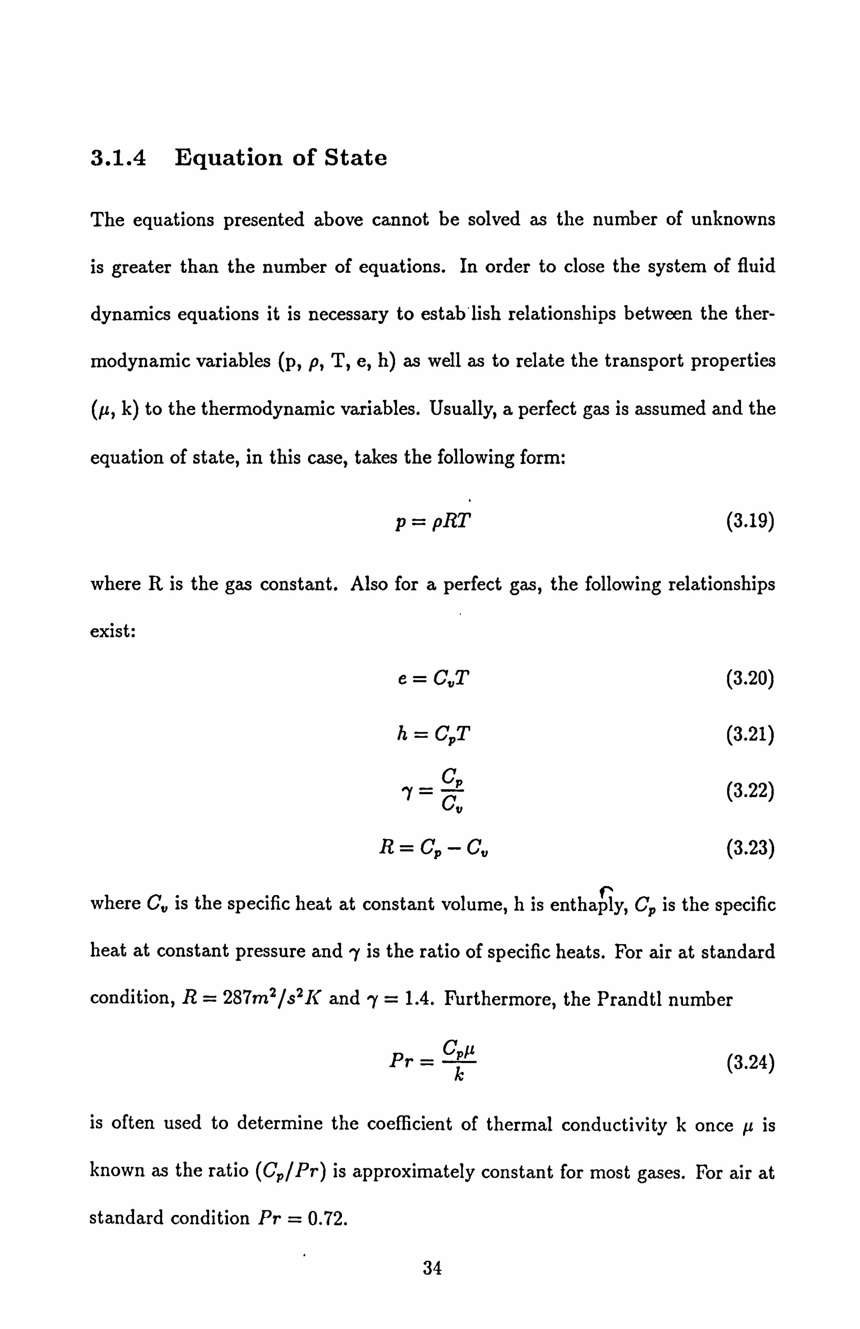
3.1.4 Equation of State
The equations presented above cannot be solved as the number of unknowns
is greater than the number of equations. In order to close the system of fluid
dynamics equations it is necessary to establish relationships between the ther-
modynamic variables (p, p, T, e, h) as well as to relate the transport properties
(p, k) to the thermodynamic variables. Usually, a perfect gas is assumed and the
equation of state, in this case, takes the following form:
p=pRT (3.19)
where R is the gas constant. Also for a perfect gas, the following relationships
exist:
e= C�T (3.20)
h=CPT (3.21)
C ry = C, v (3.22)
R=Cp - C� (3.23)
where C. is the specific heat at constant volume, h is enthap y, Cp is the specific
heat at constant pressure and y is the ratio of specific heats. For air at standard
condition, R= 287m2/s2K and ry = 1.4. Furthermore, the Prandtl number
Pr= k
(3.24)
is often used to determine the coefficient of thermal conductivity k once p is
known as the ratio (Cp/Pr) is approximately constant for most gases. For air at
standard condition Pr = 0.72.
34

3.2 Time-Averaging Procedure
The time-averaging procedure, following Reynolds, involves the decomposition of
instantaneous dependent variables into a time-averaged component plus a fluc-
tuating component about the average, i. e.
=+V (3.25)
where stands for u, v, w, p, p, T. For convenience, the mean value will be
denoted with capital letters and the fluctuating component will be denoted with
small letters hereafter. For example, U is the mean value of the velocity compo-
nent in the x-coordinate direction while u is the corresponding fluctuating part.
Substitute the above relation into the continuity and momentum equations and
then the entire equations are time averaged yields the following averaged equa-
tions in tensor form as:
+ T(PU:
+ P'u: =0 (3.26)
a_ a OP a Y (PUt + P'ut + Oxý (PU, U +U p'ui) äx ý' äx (T, i -Ujip'ui -- Pu. ui - P'usui) i
(3.27)
where the stress tensor is
ä2; ax; 3 sij aXk
where ö; j is the Kronecker delta function (Sj =1 if i=j and 5q =0 if i 54 j). For
incompressible flows the above equations reduce to:
i (PUS) =0 (3.29)
35

ät (Pui) +ä (PU; U1) _ -äP +ä (3.30)
where pu; u3 is the so called Reynolds stress and T; ý takes the following simpler
form:
Ti'_µIOu; +au; (3.31) axi ax; J
Apart from simple time-averaging, there is another approach to averaging
the equations which is called mass-weighted averaging. For the treatment of
compressible flows and mixtures of gases in particular, mass-weighted averag-
ing is convenient as the averaged equations take a simpler form than the time-
averaged equations. More details about mass-weighted averaging can be found
in (25,66,67,68).
3.3 Turbulence Modelling
The need for turbulence modelling was pointed out in chapter one. In order to
predict turbulent flows by solving the time-averaged equations it is necessary to
make closure assumptions for the unknowns which appear in the equations due to
the averaging procedure. Most of the turbulence models developed so far are for
incompressible flows, i. e., density is constant. In this case, the unknowns in the
averaged momen tumequations are the six Reynolds stresses. The discussions here
will focus on the modelling of the Reynolds stresses and some other approaches
to turbulence modelling will be also briefly introduced.
Boussinesq (69) proposed that the apparent turbulent stresses might be re-
lated to the rate of mean strain through an apparent scalar turbulent or "eddy"
36

viscosity. Although this concept was proposed more than one hundred years ago
it is still widely used in turbulence models today. For incompressible flows, the
Reynolds stresses can be expressed using the Boussinesq assumption as:
äu; öu; 2 Pu"u, = Pt
(ax; + öx; 3a`'Pk
(3.32)
where j is the turbulent viscosity and k is the averaged kinetic energy of tur-
bulence, k=u; u; /2. The problem is how to find lit when the above relation is
employed.
There are several ways of classifying turbulence models. One way is to divide
them into two categories according to whether the Boussinesq assumption is
used or not. Models using the Boussinesq assumption will be classified into
category one or called turbulent viscosity models. Most models currently used in
engineering caculations are of this type and experimental evidence indicates that
the turbulent viscosity hypothesis is valid in many flow situations. There are
exceptions, however, and there is no physical basis that it holds. Other models
which obtain the Reynolds stresses from the transport equations without the
Boussinesq assumption are referred to as category two, including those known as
Reynolds stress or, more generally, stress-equation models.
Another common classification of turbulence models is according to the num-
ber of partial differential transport equations solved in addition to the mean flow
equations. It is easier to follow the discussion in this way. According to this
classification turbulence models can be grouped into the following four classes (4,
70)
37
1). Zero equation models
2). One equation models
3). Two equation models
4). Stress equation models
Models in classes 1)-3) also belong to category one according to the previous
classification which use the Boussinesq assumpton while stress equation models
in class 4) fall into category two.
The zero equation model, which does not need any transport equations for
turbulence quantities, is also called "mean field" closure (71) while classes 2)-4)
are called "transport equation" closure.
A brief introduction to turbulence modelling will be given in the following part
of this chapter although detailed consideration of modelling of turbulent flows is
beyond the scope of this thesis. A general review of turbulence models and their
applications can be found in (4,25,71,72,73,74). Bradshaw (75) describes the
interplay between the development of models and the experiments. Launder and
Spalding (76) give the mathematical concepts of turbulence models. Bradshaw
and Cebeci (77) present calculation methods for various classes of turbulent flows.
Lumley (78,79) and Launder (80) discuss the prospects for high order closure
models. Turbulence models available for the prediction of three-dimensional flows
with curvature, rotation and flow separation are reviewed by Lekshminarayana
(81). An exhaustive review of turbulence models for near-wall and low Reynolds
number flows is given by Patel et al (82).
38

3.3.1 Zero Equation Models
Zero equation models (also called algebraic models) utilize the Boussinesq as-
sumption invariably. The first and most successful turbulence model of this type
proposed by Prandtl is still among the most widely used models. For thin shear
layers the Boussinesq assumption is applied to yield:
- pü = µt äy (3.33)
where pt is the turbulent viscosity which is related to the mean velocity by the
Prandtl mixing length hypothesis as follows:
ßt = pc l2 1 ay
1 (3.34)
where CM is a constant and 1 is the so called "mixing length" that can be thought
of the distance over which particles maintain their original momentum. The
product I äy I can be interpreted as the characteristic velocity of turbulence vt
by which the above relation can be rewritten in a more general form as:
Pt = pC,, vtl (3.35)
The mixing length has to be known before performing calculations but there
is no exact method for its prediction, hence it has to be prescribed with the aid of
empirical information. Nevertheless, the mixing length model has been used for
free shear and boundary layers very successfully. However, the evaluation of 1 in
the mixing length model changes according to the type of flows being considered
and it becomes extremely difficult to evaluate 1 for recirculating flows, three-
dimensional flows etc. The incorporation of the effects of curvature, buoyancy
39
and rotation in the model is also entirely empirical. In addition, the transport
and history effects of turbulence are not accounted for. In particular, the mixing
length model may give totally wrong answer in some cases, for example, when two
dimensional or axisymmetrical internal channel flows are considered, aý =0 in
the centre, then pt will become zero by Eq. (3.34) whereas experimental evidence
indicates that this is not true.
One major motivation for developing more complex models is the observation
that the algebraic models evaluate the turbulent viscosity in terms of only local
flow parameters, yet it is generally accepted that a turbulence model should
be able to provide a mechanism by which effects upstream can influence the
turbulence structure (and viscosity) downstream. In addition, with the simplest
models ad hoc additions and corrections are frequently required to handle specific
effects, and constants need to be adjusted to deal with different classes of flows.
If the general form for the turbulent viscosity, pt = pC, 1vtl, is accepted, then a
logical way to extend the generality of turbulent viscosity models is to construct
a more complex and general function of the flow for vi and perhaps 1, which can
account for the transport and history effects of turbulence. Specific modifications
to the constants are not then required for different classes of flows.
3.3.2 One Equation Models
In order to extend the generality of the algebraic models Prandtl and Kolmogoik
suggested in the 1940s that vt be porportional to the square root of the turbulent
kinetic energy, k=U; -U; /2. As a result, the turbulent viscosity can be expressed
40

as:
pt = pColk112 (3.36)
and pt will not be zero when äy = 0. Turbulent kinetic energy is a measurable
quantity and its physical meaning is quite clear, but the problem is how to predict
it.
A transport partial differential equation for k can be derived from the Navier-
Stokes equations after some manipul&tions. However, there are some unknowns
in the exact transport equation which need to be approximated by modelling
assumptions. For instance, when two dimensional incompressible thin-shear-layer
flows are considered, the exact transport equation for k takes the following form:
Dk p 15t
ä2k = jt
y-
ä ay
(pvk' -}- Up)
äU - püv ay - it
äu Z äv\ 2 ppyj ý-
ýy
J (3.37)
The first term on the right hand side represents diffusion due to viscous action
while the second term represents diffusion due to turbulence. The third and
fourth terms represent the generation and dissipation of turbulent kinetic energy
respectively. The turbulent diffusion term is usually modelled similarly to the
Reynolds stresses expressed in Eq. (3.32)
- pvk' _ lit ak (3.38)
Prk öy
where Prk is the Prandtl number for turbulent kinetic energy (ý 1.0). The
correlation of velocity and pressure fluctuation term äy(vp) is usually neglected.
The dissipation term is modelled using turbulent kinetic energy and a length
scale in this case. The modelled equation is as follows (25):
2C32
p-=9++ µe (3.39) Dt y Prk/
j (aU)
äyý ýý
41 SHEFFIELD UMVEPý'TY

the physical interpreation of various terms on the right hand side is quite clear,
i. e., they are the diffusion, generation and dissipation terms respectively. How-
ever, the length scale 1 needs to be specified algebraically. CD 0.164 if 1 is taken
as the ordinary mixing length (25).
In one equation models, the length scale has to be specified algebraically
as in zero equation models, and hence is also flow dependent. Moreover, it is
difficult to incorporate the length scale empirically for complicated flows such as
recirculating flows, flows with separation, streamline curvature etc. Therefore,
most one equation models do not show much improvement over zero equation
models and hence they are not very popular.
3.3.3 Two Equation Models
In order to eliminate the need for specifying the length scale based on empirical
information, the two equation models employ another transport partial differen-
tial equation to predict 1.
A transport equation for 1 can be derived, in principle, from the Navier-Stokes
equations but the unknows introduced in the transport equation cannot be easily
modelled. As a matter of fact, the introduction of several drastic modelling
approximations produce a rather empirical equation for 1. However, successful
experience has indicated that it is better to solve a transport partial differential
equation for a length scale related parameter rather than for the length scale
itself. Such a parameter is generally a combination of k and 1, Z= k°la.
Quite a few two equation models have been developed using different com-
42
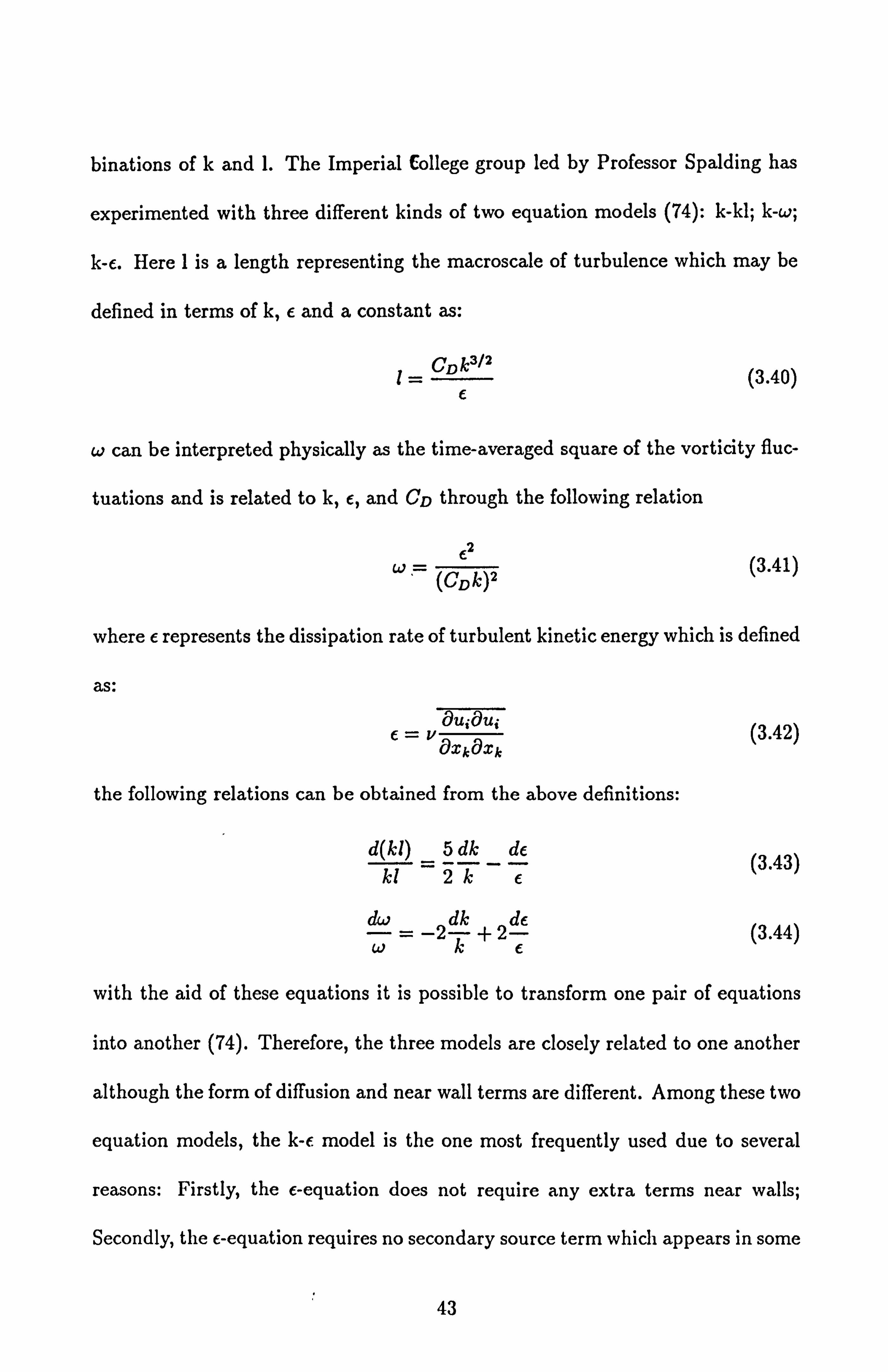
binations of k and 1. The Imperial Sollege group led by Professor Spalding has
experimented with three different kinds of two equation models (74): k-kl; k-w;
k-e. Here 1 is a length representing the macroscale of turbulence which may be
defined in terms of k, e and a constant as:
CDk312 E
(3.40)
w can be interpreted physically as the time-averaged square of the vorticity fluc-
tuations and is related to k, e, and CD through the following relation
W= (CDk)2 (3.41)
where e represents the dissipation rate of turbulent kinetic energy which is defined
as:
äu; au; vaxkaxk (3.42)
the following relations can be obtained from the above definitions:
d(kl) _5
dk de (3.43) kl 2T- e
_ -2 k
T+2- (3.44)
with the aid of these equations it is possible to transform one pair of equations
into another (74). Therefore, the three models are closely related to one another
although the form of diffusion and near wall terms are different. Among these two
equation models, the k-E model is the one most frequently used due to several
reasons: Firstly, the e-equation does not require any extra terms near walls;
Secondly, the e-equation requires no secondary source term which appears in some
43

other models. Moreover, e itself appears in the k-equation, which is convenient
as less modelling work is needed for the k-equation.
An exact transport equation for e can be derived from the Navier-Stokes
equations (84,85) and can be modelled by analogy with that of the k-equation.
The modelled transport equations for k and e with viscous diffusion presumed
negligible are given below (74):
Dk
__ a (ý= ak 1 (au; auk) au; J+ µt axk + ax;
) axk - pý (3.45) p Dt axk
[\Pr_) _ axk
DE -a it aE au; auk au; E2 + Cott! +- Cep- (3.46) pDt axk
ýýPrýý axk k axk ax; axk k -()
and the turbulent (eddy) viscosity is related to k and e as follows:
2 Ft=cip
kf (3.47)
the constants in these equations take the following values (74)
C, 4=0.09 C1=1.44 C2 = 1.92 Prk=1.0 PrE=1.3
These constants are not changed, generally speaking, in any calculations.
Nevertheless, they need to be adjusted in order to account for effects such as
streamline curvature, low Reynolds number etc.
It is necessary to point out at this stage that the above transport equations for
k and e are not appropriate for the near wall region, i. e., in the viscous sublayer
where the Reynolds number is very low and molecular transport becomes more
important. Thus, most applications of the k-e model (and other models) have
made use of wall functions which will be presented in chapter five. Alternatively,
additional terms can be put into the k and e equations to extend their applicability
to the viscous sublayer (86).
44

At present, the two equation k-e model is the most popular one for engineer-
ing calculations. However, this model (and all other two equation models as well)
have several limitations. Firstly, all two equation models are turbulent viscosity
models which assume that the Boussinesq assumption holds. The two equation
models fail if the Boussinesq assumption fails. Nevertheless, in many flow situa-
tions the assumption gives results accurate enough for engineering calcualtions.
Another practical limitation is the assumption of isotropic eddy viscosity, i. e., the
same values of pt are taken for different u; u7 terms as can be seen from Eq. (3.32)
while experimental evidence indicates that pt takes different values for different
u; u7 terms in certain cases such as strongly swirling flows. Moreover, the effects
of curvature, rotation and buoyancy forces have to be modelled separately. In
order to eliminate these limitations the so called stress equation models have been
developed.
3.3.4 Stress Equation Models
In the stress equation models, the turbulent viscosity hypothesis is not employed
and a partial differential transport equation is developed for each component
of the Reynolds stresses. In addition, the transport equation for turbulent ki-
netic energy dissiaption rate e is also needed. The stress equation models include
Reynolds stress models which solve the transport equations for the Reynolds
stresses directly through modelling assumptions, and algebraic stress models in
which an algebraic relation is derived from the Reynolds stress transport equa-
tions through some modelling assumptions. The stress equation models are also
45
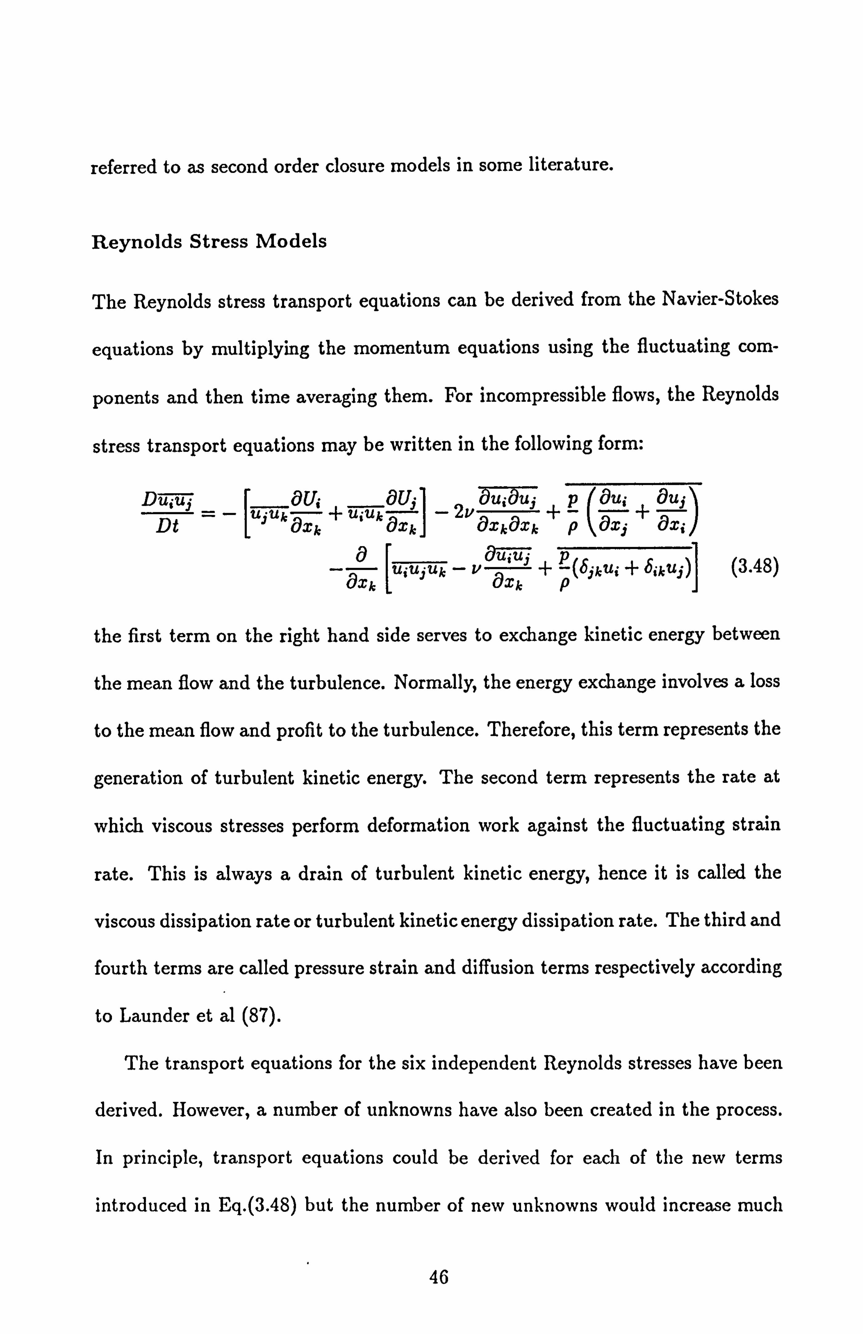
referred to as second order closure models in some literature.
Reynolds Stress Models
The Reynolds stress transport equations can be derived from the Navier-Stokes
equations by multiplying the momentum equations using the fluctuating com-
ponents and then time averaging them. For incompressible flows, the Reynolds
stress transport equations may be written in the following form:
aU u; u au; D- -uu
au + uuk ' 2v '+p+
auj Dt ' kaxk OXk, - aXkaxk p
(Oxj
a2;
a o-uiuj äxk
(uiZLjuk
-v ax +
ý(Öjk2li'i Öikuj)I (3.48)
L
the first term on the right hand side serves to exchange kinetic energy between
the mean flow and the turbulence. Normally, the energy exchange involves a loss
to the mean flow and profit to the turbulence. Therefore, this term represents the
generation of turbulent kinetic energy. The second term represents the rate at
which viscous stresses perform deformation work against the fluctuating strain
rate. This is always a drain of turbulent kinetic energy, hence it is called the
viscous dissipation rate or turbulent kinetic energy dissipation rate. The third and
fourth terms are called pressure strain and diffusion terms respectively according
to Launder et al (87).
The transport equations for the six independent Reynolds stresses have been
derived. However, a number of unknowns have also been created in the process.
In principle, transport equations could be derived for each of the new terms
introduced in Eq. (3.48) but the number of new unknowns would increase much
46
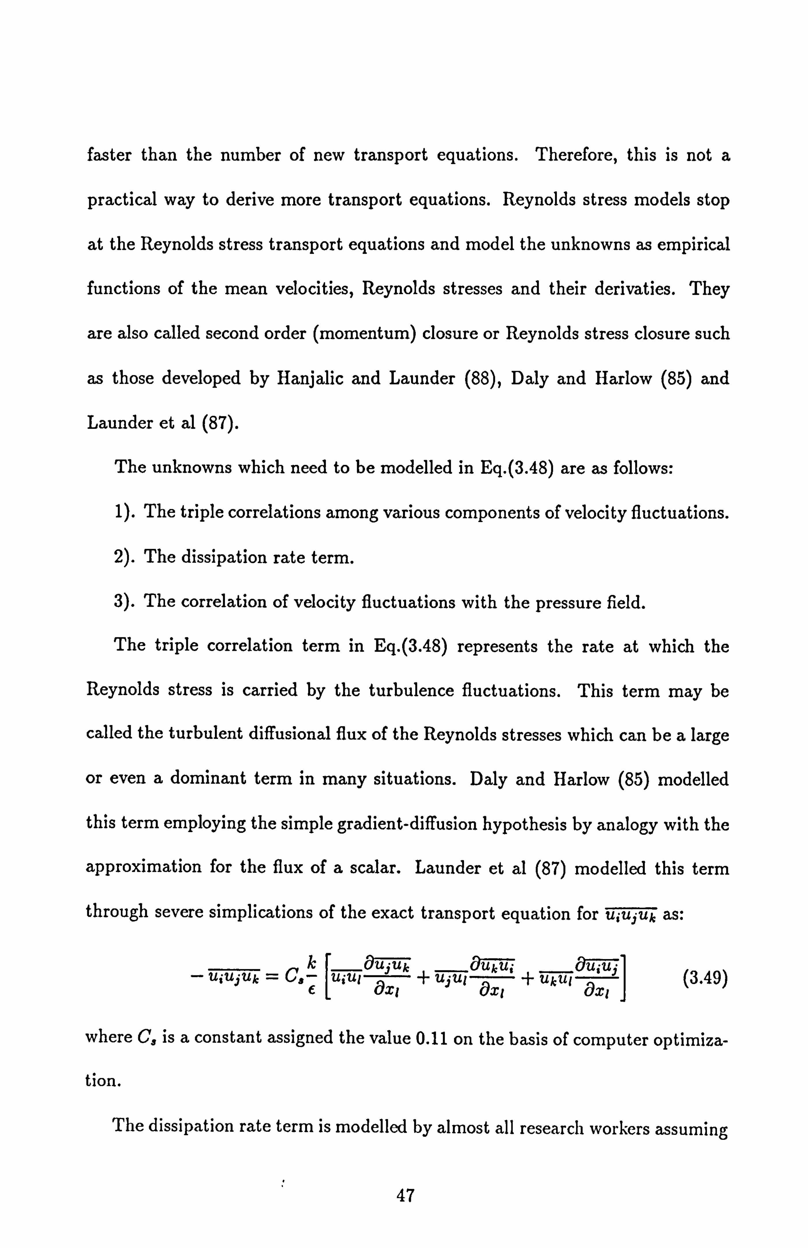
faster than the number of new transport equations. Therefore, this is not a
practical way to derive more transport equations. Reynolds stress models stop
at the Reynolds stress transport equations and model the unknowns as empirical
functions of the mean velocities, Reynolds stresses and their derivaties. They
are also called second order (momentum) closure or Reynolds stress closure such
as those developed by Hanjalic and Launder (88), Daly and Harlow (85) and
Launder et al (87).
The unknowns which need to be modelled in Eq. (3.48) are as follows:
1). The triple correlations among various components of velocity fluctuations.
2). The dissipation rate term.
3). The correlation of velocity fluctuations with the pressure field.
The triple correlation term in Eq. (3.48) represents the rate at which the
Reynolds stress is carried by the turbulence fluctuations. This term may be
called the turbulent diffusional flux of the Reynolds stresses which can be a large
or even a dominant term in many situations. Daly and Harlow (85) modelled
this term employing the simple gradient-diffusion hypothesis by analogy with the
approximation for the flux of a scalar. Launder et al (87) modelled this term
through severe simplications of the exact transport equation for u; u,, uk as:
u uk u; u t ý] (3.49) - utujuk = Cak
el
ru'ut äxt + uýut ex t+
akut äx
where C, is a constant assigned the value 0.11 on the basis of computer optimiza-
tion.
The dissipation rate term is modelled by almost all research workers assuming
47

that the dissipation motions are isotropic
öXk/ 3sij. (3.50) 2vlOXk/
(auj\
Although experimental evidence has shown that turbulence does not remain lo-
cally isotropic in the presence of strong strain fields Eq. (3.50) seemed to be the
best of the simple hypotheses.
The pressure-induced diffusion in the diffusion term in Eq. (3.48) was repre-
sented as a simple diffusion term by Daly and Harlow (85). However, Launder et
al (87) stated that it was usually neglected following the practice of most other
workers although there seemed to be no direct evidence to sustain or demolish
the assumption.
The only remaining term to be modelled is the pressure-strain correlation
which is of particualr importance for anistropic turbulence and seems to be the
most difficult to model. The appropriate starting point is to derive a Poisson
equation for mean and fluctuating pressure from the momentum equations, which
represents pressure as a function of the velocity field. This transforms the problem
to one in which only multiple velocity correlations are involved. For isothermal
incompressible flow, the Poisson equation for pressure is
_ V2(P p) __
av au 02u; u TI, _U; p+
2ax1 ax; + ax; ax;
+ 7x; a-KL
(3.51)
integrating the above equation by Green's formula yields the following expression
for pressure:
1 P(xo, yo, zo) + p(xo, yo, zo) _- --
fffV 2(p + p) d Vol
+S (3.52) 4r r
48

where S is a surface integral which is negligible away from the solid boundary and
hence is neglected hereafter. Multiplying both sides of Eq. (3.52) by (ä±e
and taking the time average, the pressure-strain correlation may be re-expressed
in the following form:
p öu' +
auj _ 4ýij, i + ß; i, 2 (3.53)
p
(8x, 8x;
1% ä2ulum öu, 8uj dVol 3.54 = 4ir J{
(49XIOX
M/ \axi + axi)
Ir()
2% aui '' äu; äu; dVol ) ýýý, z - 4r J (äxm) (Lum
aX -/\ axj + ax: )
r (3.55
where the prime superscript indicates that the quantity involved is evaluated at
a distance r from the one in question. ß; J, 1 involves only fluctuating quantities
and ß; j, 2 involves products of turbulence quantities and the mean rates of strain.
These two parts are modelled separately by almost all the research workers. ß; j, 1
is referred to as the "return-to-isotropy" term as it serves to interchange turbu-
lence energy among the various components, i. e., equaling the normal Reynolds
stresses and diminishing shear stresses. This term has significant influence for
problems involving anisotropic homogeneous flow where the mean velocity is small
or zero. A closure approximation for -O; j, 1 as first proposed by Rotta (89) and
adopted by most workers may take the following form:
ýti, l = -Cl k (utui -3 S12 k) (3.56)
This form is consistent with the assumption that the rate of return to isotropy
is directly proportional to the anisotropy (the term in brackets in the above
equation). Details about modelling the second part, 1; j, 2, can be found in (78,87,
49

88). Most workers adopt Rotta's proposals for this term and the final expression
takes the form (87):
(C2+8)lpi 2p8i] -(30C2-2)ku; +a"' 11 '3' 55 axj ax;
- (8C2 2) [Gii -3 PS ] (3.57)
11
where P; j [u; uk a+ uJuk
], G;; [U uk + 77 ä]. P represents
the rate of turbulent kinetic energy production. Launder et al argued that the
first group on the right hand side in Eq. (3.57) was the dominant one, and as a
result the equation was expressed in a simplified form as:
3 P51) (3.58)
where -y is a constant whose value is around 0.6, P;, and P are the same production
terms given before. The above equation is employed in the present study.
Near wall effects have not been taken into account in the modelling process so
far. A wall reduces the fluctuating velocity components normal to the wall and
enhances those parallel to it. The pressure-strain term, as stated before, serves to
redistribute turbulence energy among the Reynolds stresses. Thus, it would not
be appropriate to neglect the surface integral in Eq. (3.52) in the region near a
wall. It has been suggested by various workers that near wall corrections should
be incorporated into the expression for ß; j, 1 and ß; j, 2. The final form of near wall
correction to the pressure-strain given by Launder et al (87) is as follows:
2 k3/2 <> , j�� =
[o. 125(W - 3ö;; k) +0.015(P, 2 - Gii)]
ex (3.59)
i
where xl is the normal distance to the surface of a wall. Upon rearranging all the
modelled terms the final expression for the modelled Reynolds stress transport
50

equations may be written in Cartesian tensor form as:
D 7i [Ti ay; l e2 Dt =- ukaxk +uiUkaxk j- 3S, je - Clk(uýui - 3öijk)
uýuý u uý
uku` -ý- ukul
u`uj (3.60) i, axk E
[u-iul
-Ht's -I- ý; w+ co a--
ka ex i' ax, ax,
where Cj, 2is given by Eq. (3.57) or Eq. (3.58), 4D; j,,,, is the near wall correction
given by Eq. (3.59). The above equation can be also written in a compact form
as:
DDt' = Pu -
3S;; e + ý, i + Dij (3.61)
where
P; 3 - Production tensor (3.62)
4)ij = Pressure - strain tensor (3.63)
D;, -Diffusion tensor (3.64)
In order to solve the above equation one needs to know the turbulent kinetic
energy dissipation rate. The exact transport equation fore at high Reynolds
number is (84,87)
DE a au; 2V OP auk au; au; auk 2u; 2 Dt - a-Xk vuk
(äx, ) +pX, ä7x, -Zväxk äx ax, -2 Loo]x, (3.65)
This transport equation contains several unknowns which need to be modelled
to make the equation solvable. The modelled equation given by Hanjalic and
Launder (88) takes the following form:
De =a
(kT- a e) U; ez
Dt Cask e uu' äx, J C`ieu, ukk axk
C2 (3.66)
51

the first term on the right hand side approximates the corresponding term in
Eq. (3.64) responsible for the diffusion of e. The second and third terms represent
the generation of e and its destruction by viscous action.
The values of constants given by Launder et al (87) are as follows:
C1=1.5 C2= 0.4 C. = 0.11 ry=0.6 CC=0.15 Cc1=1.44 Ce2=1.90
Algebraic Stress Models
In Reynolds stress models there are six Reynolds stress transport equations in
addition to the transport equation for e. Solving such a set of equations needs
enormous computer time. Rodi (90,91) proposed an algebraic relation from
Eq. (3.60) for calculating the Reynolds stresses in order to reduce computational
effort. It can be seen from Eq. (3.60) that there are only two terms involving the
gradient of the Reynolds stresses, i. e., the term on the left hand side and the
difliusion term D;,, on the right. The Reynolds stress transport equations would
become algebraic equations if these two terms could be approximated involving
only algebraic relations for the Reynolds stresses by modelling assumptions. Rodi
(90,91) assumed that convective and diffusive transport of u; uI are proportional
to those of k and the proportionality factor is u; uc/k. Mathematically, these
assumptions may take the following forms:
Du; ui _
u; uj Dk Dt k Dt
(3.67)
Dsj =u ff D(k) (3.68)
where D(k) represents the diffusion of k. It is argued by Rodi that the above
assumptions are appropriate if the rate of variation of u; uj/k along a streamline
52

is much less than that of u; u� and if the spatial gradient of u; uj is large compared
with that of u; uj/k. Also, the transport equation for k can be written as:
Dk P_+ D(k) (3.69)
Dt
substituting Eq. (3.69) into Eq. (3.67), one has:
DDt =
uk' [P -e+ D(k)] (3.70)
combining Eq. (3.68) and Eq. (3.70) with Eq. (3.61) yields an algebraic equation
for u; uJ in tensor form as:
uk' (P - e) = P;; - 3öu;
e +4;; (3.71)
as k and e appear in the above equation so k and e equations need to be solved
as well.
Invariance and Realizability
The ideal turbulence models should have general applicability and be flow inde-
pendent. The development of Reynolds stress models is a step towards this ideal
as more physical processes such as those due to curvature, rotation, buoyancy,
and so on, can be accounted for automatically. For general applicability it has
been shown (78,79,92,93) that these models have to satisfy many constraints.
Tensor invariance requires the replaced terms to have the same tensor form as the
original terms so that they can be transformed properly in different coordinate
systems. This type of modelling is called invariant modelling (92). The concept
of realizability was first introduced by Schumann (93). Ile stated that no matter
53

what equation is used to predict u; ui it must have the property which does not
allow negative component energies and requires all off diagonal components of the
Reynolds stress to satisfy Schwartz's inequality. These and the additional con-
ditions put forth by Schumann can be written in a numerically most convenient
form as (93):
Rll>0 (3.72)
R11R22 - Rig >0 (3.73)
Ril(R22R33 - Rz3) - Rl2(Rl2R33- R23Rl3) + R13(Rl2R23 - R22R13) >0 (3.74)
Similar conditions apply for scalar fluxes. Schumann shows that the exact Reynolds
stress transport equations satisfy the realizability condition. However, it is also
indicated by him that some of the existing models do not satisfy such a condi-
tion. Nevertheless, attempts to satisfy the realizability condition lead invariably
to complicated model expressions. Therefore, at present no special efforts are
taken to ensure that models satisfy the realizability condition.
There is no doubt that stress equation models are relatively more general
than other models discussed previously. They are not restricted by the Boussi-
nesq assumption relating turbulent stresses to the rate of mean strain. However,
approximations and assumptions are still used in modelling various terms which
presently cannot be measured. Moreover, Reynolds stress models have not been
well tested for many types of complex flows and it may take some time before they
have been fully tested and refined to the point that they become commonplace
in engineering calculations.
54
3.3.5 Multiple-Scale Models
It is recongized that fully developed turbulence (when Reynolds number is well
above the critical value) consists of fluctuating motion with a wide spectrum
of eddy size and time scales. For instance, in turbulent pipe flow the largest
turbulence eddies are of a size comparable with the diameter of the pipe while the
smaller eddies are so small that viscous action becomes dominant. The large-scale
eddies contain much of the kinetic energy of turbulence and dissipate little energy
by viscous effects. These large-scale eddies interact with each other, generating
smaller eddies in which viscous dissipation becomes important. Since different
turbulent interactions are associated with different parts of the spectrum it would
be desirable to have turbulence models accounting for this detailed structure of
turbulence. Unfortunately, all the turbulence models discussed above are based
on a single-scale scheme. Hanjalic et al (94) proposed a multiple-scale model
based on a rational extension of widely used single-scale equations and ideas. An
outline of their model is briefly described below.
A typical energy spectrum of turbulence is known to consist of, generally
speaking, three regions. These are the production region (low wave number
region); the dissipation region (high wave number region) and between these two
regions, with an intermediate range of wave number, is the so called transfer
region (also called the inertial region). Since there is negligible kinetic energy
of turbulence in the dissipation region the total turbulent kinetic energy k is
assumed to comprise kp in the production region and kt in the transfer region.
Turbulent kinetic energy leaves the first region (the production region) at a rate
55

ep, enters the dissipation region at a rate e and across the transfer region at
an assumed representive spectral energy transfer rate et. This simplified energy
spectrum is the basis of the model of Hanjalic et al. They argue that the spectral
division appears to be too coarse but the single-scale models take no cognizance of
changes in the shape of the energy spectrum, and there is implicit the assumption
that Ep = Et = E. The transport equations for kp, kt, ep, et are formulated. In a
homogeneous flow the transport equations for kp and kt are (94):
Dkp _u"u
-au` (3.75) Dt `'5 p
Dkt_ Dt -ep -e (3.76)
and the transport equations for ep, et given by Hanjalic et al (94) take the following
forms: DEp
=1 eP aU;
C, p
z
2 Ep
+ DE -U, 7u
'C, p p (3.77)
Dt kp äxß kp
z DEt = Ctl EpEt
- ct2 Et + Det (3.78) Dt kt kp
where Do (0 stands for kp, kt, ep, et) is the diffusion term and can be uniformly
represented as:
D4, = 0.22-Oxk j Ep
(3.79) PJ
This model was used to predict axisymmetrical jets and boundary layers (94).
Good agreement was obtained between the prediction of the jet spread rate and
experimental data. For the boundary layers the prediction with this model is in
closer agreement with experimental data than the single-scale model of Launder
et al (87). This shows the potential advantages of including some account of the
56
spectral character of turbulence in traditional second-moment closures. However,
this model has not been tested further.
3.3.6 Other Approachs to Turbulence Modelling
Apart from the models discussed above there are some other approachs to turbu-
lence modelling such as two-point closure and large-eddy-simulation. The stress
equation models (second-order modelling), including multi-scale models, are only
one-point closure. This involves merely averaging the Navier-Stokes equations
and approximating the unknowns introduced in the averaging procedure through
modelling auusmptions. Usually, the approaches to solve turbulent flows can be
classified into three categories, i. e., one-point closure (which is the most widely
used technique so far), two-point closure and large-eddy-simulation.
Two-point closure considers differential equations for two point correlations or
the spectrum tensor. This technique is intermediate in complexity between large-
eddy-simulation (with sub-grid-scale modelling) and one-point closure (second-
order modelling). The potential advantage of the two-point closure lies in its
relative simplicity when compared with large-eddy-simulation and its flexibility
and universality when compared with the common one-point closure. In partic-
ular, it can be used to identify proper coefficients to be used in the one-point
closure.
Large-eddy-simulation has been developed recently. Deardorff (83) first sug-
gested this approach and used it to predict channel flows and atmospheric bound-
ary layers. This approach consists of averaging the Navier-Stokes equations over
57

a time T shorter than the time scale of the large turbulent structures of the
motion. Only the time-dependent fluctuations with a time scale smaller than T
are smoothed out which are then approximated by the so called sub-grid-scale
modelling. Such calculations have shown much promise. However, this tech-
nique is too costly at present to be considered as a practical way for engineering
calculations.
58

Chapter 4
SOLUTION PROCEDURE
The governing equations presented in the previous chapter are non-linear, cou-
pled, and second-order partial differential equations. The analytical solution is
formidable due to not only non-linearity but also the complex flow structure of
turbulence. Hence, a method of numerical solution has to be employed to solve
the governing nonlinear partial differential equations.
As numerical schemes and the methods to discretize the governing partial
differential equations are fairly standard and well documented (2,6,7,16,25,
64), only a brief introduction will be given in this chapter. However, the proper
differencing of the pressure gradient and the evaluation of density at the control
volume boundaries are of great importance in supersonic flow. In addition, the
treatment of velocity-pressure coupling becomes very crucial to the whole solution
procedure when pressure is chosen as a main dependent variable. Therefore, the
discussion will be focussed on these two important issues.
59

4.1 The Finite Difference Equations
The method employed to derive the finite difference equations is the control
volume approach due to its clear physical meaning. It entails dividing the com-
putational domain into a great number of finite volumes (control volumes) called
`cells'. The finite difference counterparts of the governing partial differential equa-
tions are derived for each cell by a combination of formal integration and some
approximations so as to preserve physical realism and computational stability.
A staggered grid system is employed here to avoid an unrealistic solution. All
the variables except the axial and radial velocity components are stored at the
nodes. The U and V velocity components are stored mid-way between the grid
nodes. This arrangement has the following advantages:
1). The velocities are between the pressures which drive them. This may
avoid an unrealistic pressure field.
2). The velocities are directly available for the evaluation of the convective
fluxes across the control volume boundaries of the nodes. This is also convenient
for the solution procedure adopted for the continuity equation.
The numerical scheme employed to approximate the convective terms is the
so called `hybrid scheme' which is a combination of the central- and upwind-
differencing schemes. Whether the central- or upwind- differencing scheme is
used or not depends on the local convection/diffusion ratio as measured by the
local Peclet number, defined as follows:
Pe = uP& (4.1) v
60

where v is the kinematic viscosity and Sx is the mesh increment. When the
local Pe is equal to 2 or less the central differencing scheme is used. When the
local Pe is over 2 the upwind differencing scheme is used instead of the central
differencing scheme in order to avoid numerical instability. The hybrid scheme
has been proved to be stable and superior to both the central- and upwind-
differencing schemes. Moreover, the QUICK (Quadratic Upstream Interpolation
for Convective Kinematics) differencing scheme, which is more accurate, has also
been incorporated into the computer code.
4.2 Solution of the Difference Equations
The algebraic finite difference equations obtained from the governing partial dif-
ferential equations are also non-linear and coupled and cannot be solved directly.
Hence, an iterative solution method has to be used to solve these equations. The
non-linearities are usually handled by expressing the quantities at the current
iteration level in terms of the values available at the previous iteration level. In
the present work, the non-linear algebraic finite difference equations are linearized
through the calculation of coefficients based on the currently available flow field
values. This practise results in the coefficients lagging behind by one iteration.
However, when the solution converges all the equations are satisfied and this
effect is eliminated automatically.
A form of the Gauss-Seidel line by line iteration method is then employed to
solve the linearized algebraic finite difference equations in such a way that each
61

variable is solved separately instead of a simultaneous solution of all the variables.
The variables along each grid line are calculated by the use of the Tri-Diagonal
Matrix Algorithm (TDMA) which is given in more detail in (7).
4.3 Boundary Conditions
It is believed that most of the flow patterns of common gases and liquids can be
described by the same governing partial differential equations, the Navier-Stokes
equations. The flows (solutions) are distingushed only by boundary and initial
conditions, and by the flow parameters such as Re, Pr etc. It is therefore under-
standable that the specification of the computational boundary conditions plays
a very crucial role in the solution procedure. The proper specification of the
boundary conditions, apart from affecting numerical stability, greatly affects the
accuracy of the solution of the finite difference equations. This is of great im-
portance to compressible flow as the mathematical theory for the computational
boundary conditions is not so well established for the compressible Navier-Stokes
equations as it is for the incompressible form of the governing equations.
For confined flow, the boundaries can be classified, generally speaking, into
four categories:
1). Inlet (Inflow) boundary,
2). Wall boundary,
3). Symmetry boundary,
4). Outlet (outflow) boundary.
62

Wall and symmetry boundaries can be also grouped as no-flow boundaries,
i. e., the fluid cannot cross this kind of boundary.
The slip and no-slip wall boundary conditions are usually used for inviscid
and viscous flows resprectively. More detailes can be found in (2).
Across a symmetry surface the reflection method is usually adopted, e. g., if a
line of node points j=s are on the line of symmetry, one has
V"-i =-V, +i (4.2)
V, =0 (4.3)
Fd-i = Fs+1 (4.4)
where F=p, U, W or T etc.
The treatment of the inlet and outlet boundary conditions, especially for com-
pressible flow, is very important but the established treatment of outlet boundary
conditions for supersonic flow is misleading. This will be discussed in more detail
in chapter six.
4.4 Treatment of Velocity-Pressure Coupling
It was pointed out previously that when pressure is chosen as a main dependent
variable the difficulty is how to evalute pressure as there is not a governing equa-
tion for pressure in the original set of equations. However, there are several ways
of calculating pressure indirectly, such as the Poisson equation method, which
have been discussed in chapter two. Among these methods, pressure correction
63

methods have gained more favor than the others and found wide application.
In this section, the pressure correction method for incompressible flow used in
the present study will be briefly outlined and its extension to compressible flow
presented.
4.4.1 The SIMPLE Algorithm
The obstacle arising from the choice of pressure as a main dependent variable
can be removed by devising a mechanism by which the continuity and momen-
tum equations are linked together to evaluate pressure. The basic idea of pressure
correction methods is to first guess a pressure field, then get an approximate so-
lution to the velocity field. The velocity field obtained using the guessed pressure
field does generally not satisfy the continuity equation, and corrections to the
pressure field are made in such a way so as to bring the velocity field into con-
formity with the continuity equation. The key point of this is approach to derive
a so called pressure-correction equation from the finite difference form of the
continuity and momentum equations. In the present study, the pressure correc-
tion method employed is the SIMPLE (Semi-Implicit Method for Pressure-Linked
Equations) algorithm proposed by Pantakar and Spalding (6,7) which is outlined
for the two dimensional case as follows:
1). Guess the initial values of the flow field variables, which are usually
specified as zero.
2). The following momentum equations are solved using the guessed pressure
64
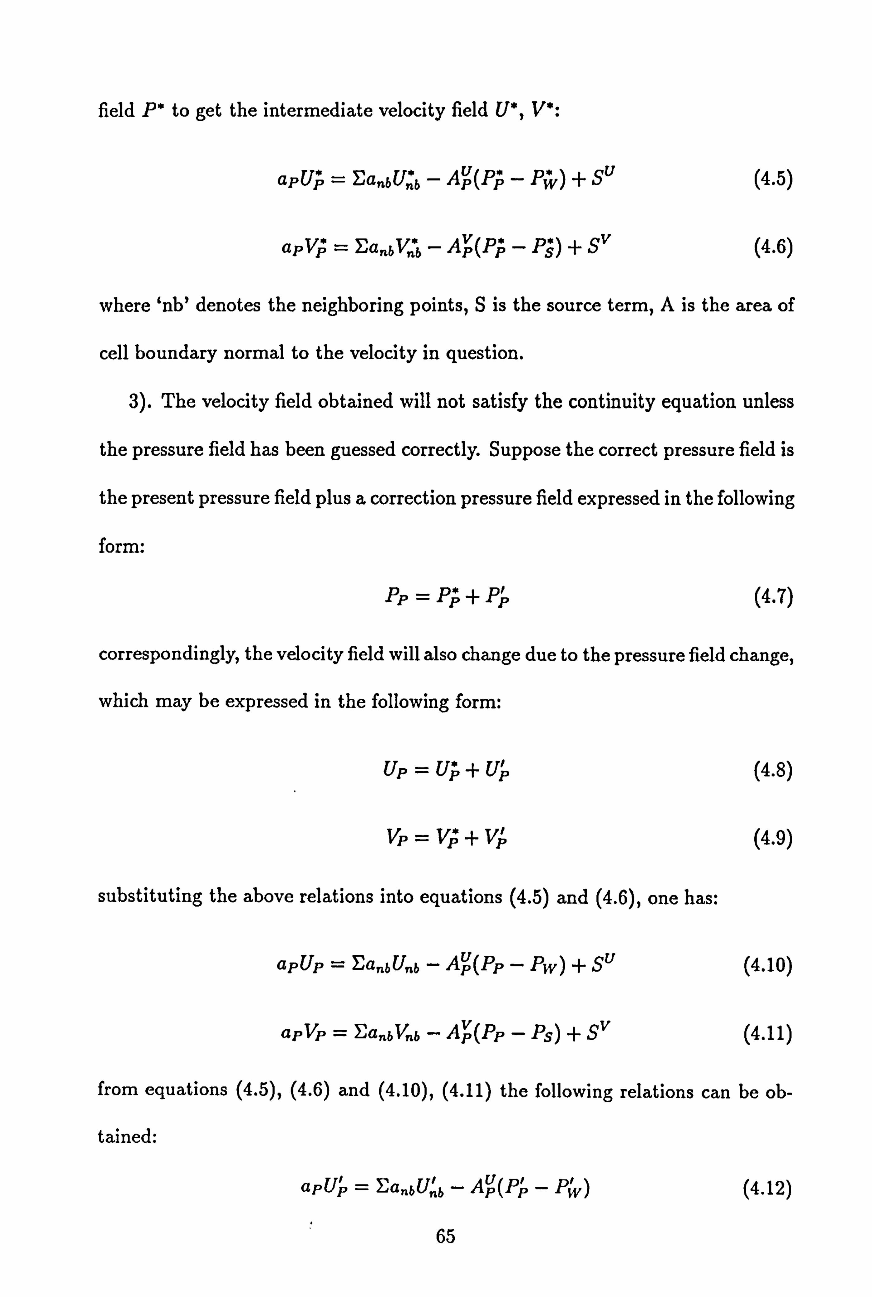
field P* to get the intermediate velocity field U*, V *:
apUU = Ea,, bUnb - AP (PP - Pw) + SU (4.5)
aPVP = Ean6Vri6 - AP(PP - Ps) + Sv (4.6)
where `nb' denotes the neighboring points, S is the source term, A is the area of
cell boundary normal to the velocity in question.
3). The velocity field obtained will not satisfy the continuity equation unless
the pressure field has been guessed correctly. Suppose the correct pressure field is
the present pressure field plus a correction pressure field expressed in the following
form:
PP = PP -I- PP (4.7)
correspondingly, the velocity field will also change due to the pressure field change,
which may be expressed in the following form:
up =UP+UP (4.8)
Vp = Vj + Vj (4.9)
substituting the above relations into equations (4.5) and (4.6), one has:
apUp = Ea bU b- AU(PP - Pw) + SU (4.10)
apVp = EanbVnb - AV (Pp - Ps) + Sv (4.11)
from equations (4.5), (4.6) and (4.10), (4.11) the following relations can be ob-
tained:
apU, = FQn6Unb - AP(ý'P - Pw) (4.12)
65

apVP = FQn6Vnb - AP( Pp - Ps) (4.13)
neglecting EanbU, b and EanbVnb, the relationship between the pressure change
and the corresponding velocity change can be expressed as follows:
UP = DP(Ptiy - PP) (4.14)
Vp = DP (Ps - Pr) (4.15)
D p, Dp can be evaluated from the relevant momentum equations:
D° = 4/a4 (4.16)
DP = AP/av (4.17)
4). P is calculated from the pressure-correction equation which is derived as
follows:
subsituting the following relations
UP = UP + DP(Pw - Pp) (4.18)
VP = VP + DP GPs - Pp) (4.19)
into the finite difference form of the continuity equation and after some manipu-
lation, the resultant pressure-correction equation is:
apPP = awPPv + aEPE + aNPiv + asPP + So (4.20)
aw = PwAwDu (4.21)
aE = PeAEDE (4.22)
as = P. AsDs (4.23)
66
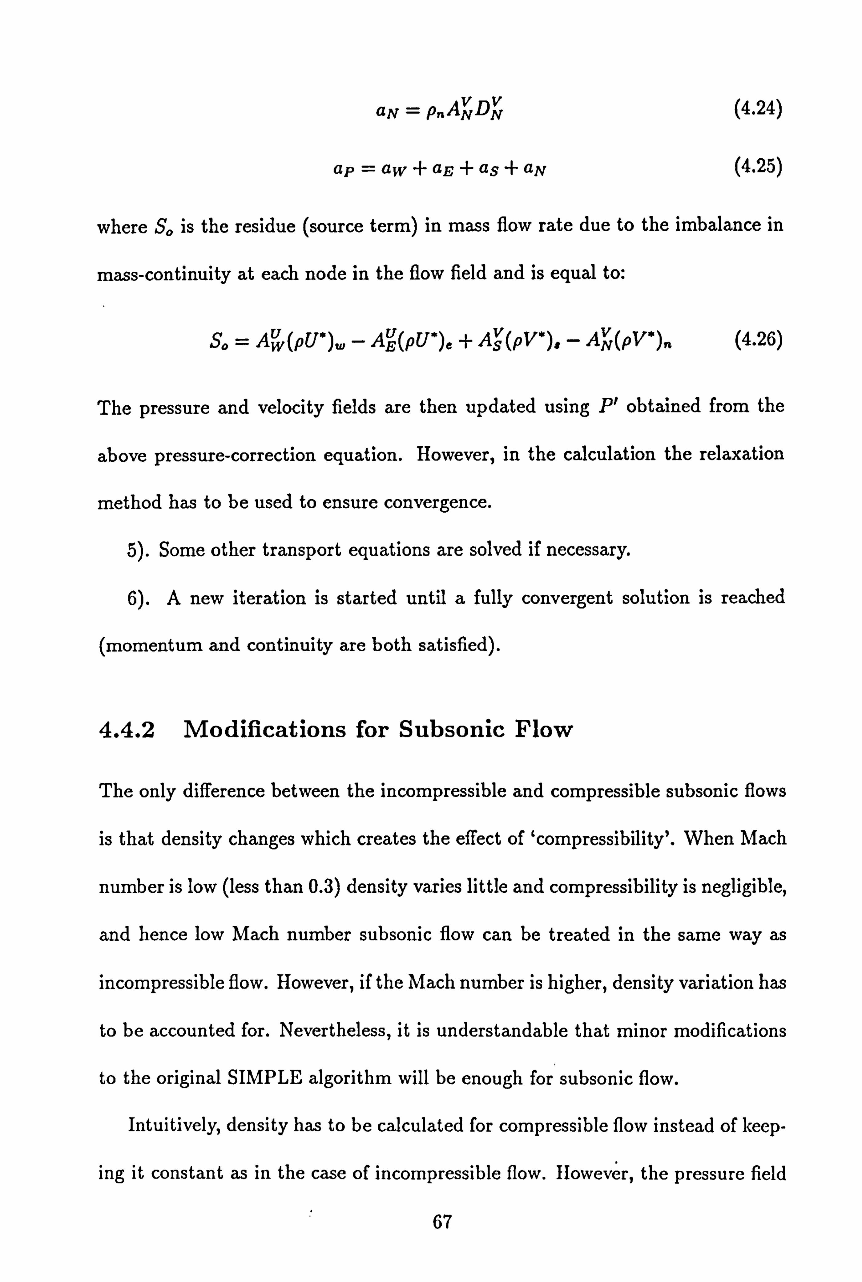
aN =p ANDN (4.24)
ap=aw+aE+as+aN (4.25)
where So is the residue (source term) in mass flow rate due to the imbalance in
mass-continuity at each node in the flow field and is equal to:
So = AU (pU*)+o - AU(PU*)e + AS (pV *), - AN(PV *)n (4.26)
The pressure and velocity fields are then updated using P obtained from the
above pressure-correction equation. However, in the calculation the relaxation
method has to be used to ensure convergence.
5). Some other transport equations are solved if necessary.
6). A new iteration is started until a fully convergent solution is reached
(momentum and continuity are both satisfied).
4.4.2 Modifications for Subsonic Flow
The only difference between the incompressible and compressible subsonic flows
is that density changes which creates the effect of `compressibility'. When Mach
number is low (less than 0.3) density varies little and compressibility is negligible,
and hence low Mach number subsonic flow can be treated in the same way as
incompressible flow. However, if the Mach number is higher, density variation has
to be accounted for. Nevertheless, it is understandable that minor modifications
to the original SIMPLE algorithm will be enough for subsonic flow.
Intuitively, density has to be calculated for compressible flow instead of keep-
ing it constant as in the case of incompressible flow. However, the pressure field
67

obtained using the SIMPLE algorithm is based on an arbitrary pressure at the
specified reference point, and usually it is set equal to zero. Therefore, the pres-
sure field cannot be used to calculate density directly unless the correct pressure is
given at the specified reference point. As a result, one important step is to specify
a correct pressure for compressible subsonic (the same for supersonic) flow. This
pressure is given'either experimentally or analytically. Moreover, if temperature
needs to be calculated then the transport equation of stagnation enthalpy should
be solved. The calculation of density is switched on using the gas state law after
a reasonable pressure field is established, i. e., after a certain number of iterations
so as to avoid an unrealistic pressure field since negative pressure may be present
at the very begining of calculation. The modified solution procedure is then as
follows:
1). - 4). The same as before,
5). The transport equation of stagnation enthalpy is solved to get the tem-
perature field.
6). The calculation of density is switched on after a certain number of itera-
tions.
7). Some other transport equations are solved if necessary.
8). A new iteration is started until a fully convergent solution is reached.
It has been found that the modified solution procedure performs quite well
for subsonic flow in several cases. It can be claimed with confidence that the
modified solution procedure can handle subsonic flow in general if the computa-
tional boundary conditions are specified properly. This aspect will be discussed
68
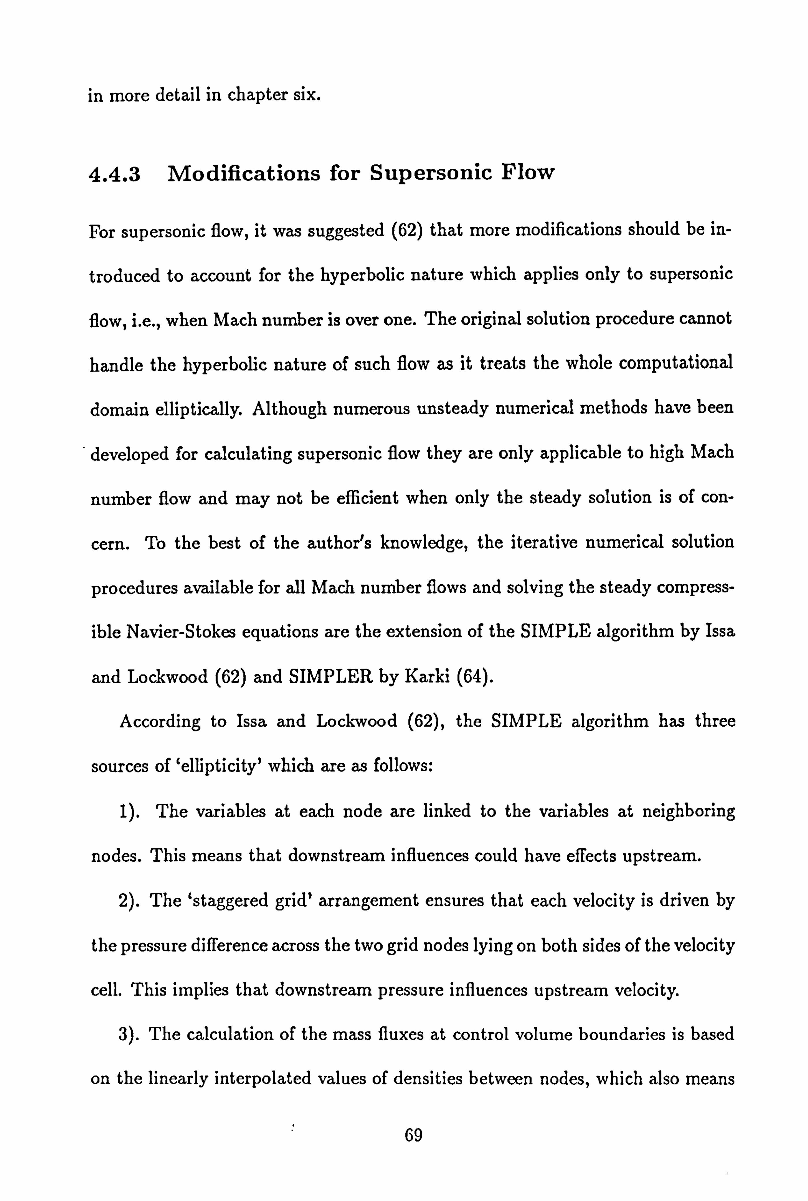
in more detail in chapter six.
4.4.3 Modifications for Supersonic Flow
For supersonic flow, it was suggested (62) that more modifications should be in-
troduced to account for the hyperbolic nature which applies only to supersonic
flow, i. e., when Mach number is over one. The original solution procedure cannot
handle the hyperbolic nature of such flow as it treats the whole computational
domain elliptically. Although numerous unsteady numerical methods have been
developed for calculating supersonic flow they are only applicable to high Mach
number flow and may not be efficient when only the steady solution is of con-
cern. To the best of the author's knowledge, the iterative numerical solution
procedures available for all Mach number flows and solving the steady compress-
ible Navier-Stokes equations are the extension of the SIMPLE algorithm by Issa
and Lockwood (62) and SIMPLER by Karki (64).
According to Issa and Lockwood (62), the SIMPLE algorithm has three
sources of `ellipticity' which are as follows:
1). The variables at each node are linked to the variables at neighboring
nodes. This means that downstream influences could have effects upstream.
2). The `staggered grid' arrangement ensures that each velocity is driven by
the pressure difference across the two grid nodes lying on both sides of the velocity
cell. This implies that downstream pressure influences upstream velocity.
3). The calculation of the mass fluxes at control volume boundaries is based
on the linearly interpolated values of densities between nodes, which also means
69

that the downstream pertubations can be transmitted upstream.
Issa and Lockwood argued that modifications should be introduced to elim-
inate these downstream influences so as to make the solution procedure able to
handle the hyperbolic nature of supersonic flow.
The first elliptical numerical influence is automatically eliminated due to
the use of a hybrid differencing scheme which employs an upwind differencing
scheme for the convective terms and ingores diffusional effects when the con-
vection/diffusion ratio is large. This is definitely satisfied for supersonic flow.
Therefore there is no need to introduce any modification for the first elliptical
source.
With respect to the second elliptical influence, this was done (62) in such a
simple way that the pressure difference across the adjacent two upstream nodes
was taken instead of the two nodes lying on both sides of the velocity. For
example, the unmodified pressure gradient (P(I, J) - P(I - 1, J))/Sx for the
velocity U(I, J) will be (P(I - 1, J) - P(I - 2, J))/8x after modification. This
treatment of the pressure gradient is doubtful and will be discussed later.
The third elliptical effect was removed by using only upstream densities when
the supersonic fluxes were calculated, i. e., density was upwinded when supersonic
mass fluxes were calculated.
Karki (64) also argued that the evaluation of density at the control volume
boundaries and the differencing of the pressure gradient were two very critical
issues, which determined the validity of a solution procedure in the transonic
and supersonic flow regions. These two very important issues are actually the
70

second and third elliptical sources as defined by Issa and Lockwood (64). Their
argurements, not surprisingly, are exactly the same bearing in mind that the
first elliptical source can be eliminated automatically by the use of the hybrid
differencing scheme. The difference is how they modified the solution procedure
to account for these effects.
For the third elliptical source, i. e., how to evaluate density at the control
volume boundaries, upstream densities were used for the supersonic mass flux
calculations in Issa and Lockwood's modified solution procedure as mentioned
above. It was shown by Karki (64) that using an upwind biased density was
equivalent to the effect of adding the artificial viscosity. Bearing this in mind, it
is understandable why upstream densities are used for the supersonic mass flux
calculations. However, Karki (64) also argued that the use of two different meth-
ods to evaluate density for subsonic and supersonic flow respectively might cause
some numerical problems near the switch-over point, and the switch-over point
itself might be problem dependent. Therefore, density was always upwinded no
matter what the Mach number was in Karki's modified solution procedure. This
treatment seems to provide enough numerical diffusion but also adds damping
even in subsonic flow regions where it is not required. In the present study, den-
sity is therefore upwinded only when local Mach number is over one, and it has
been found that this treatment does not cause any problem near the switch-over
point.
The second elliptical source, i. e., the treatment of the pressure gradient, seems
to be quite confusing. The hyperbolic nature of supersonic flow tells us that small
71
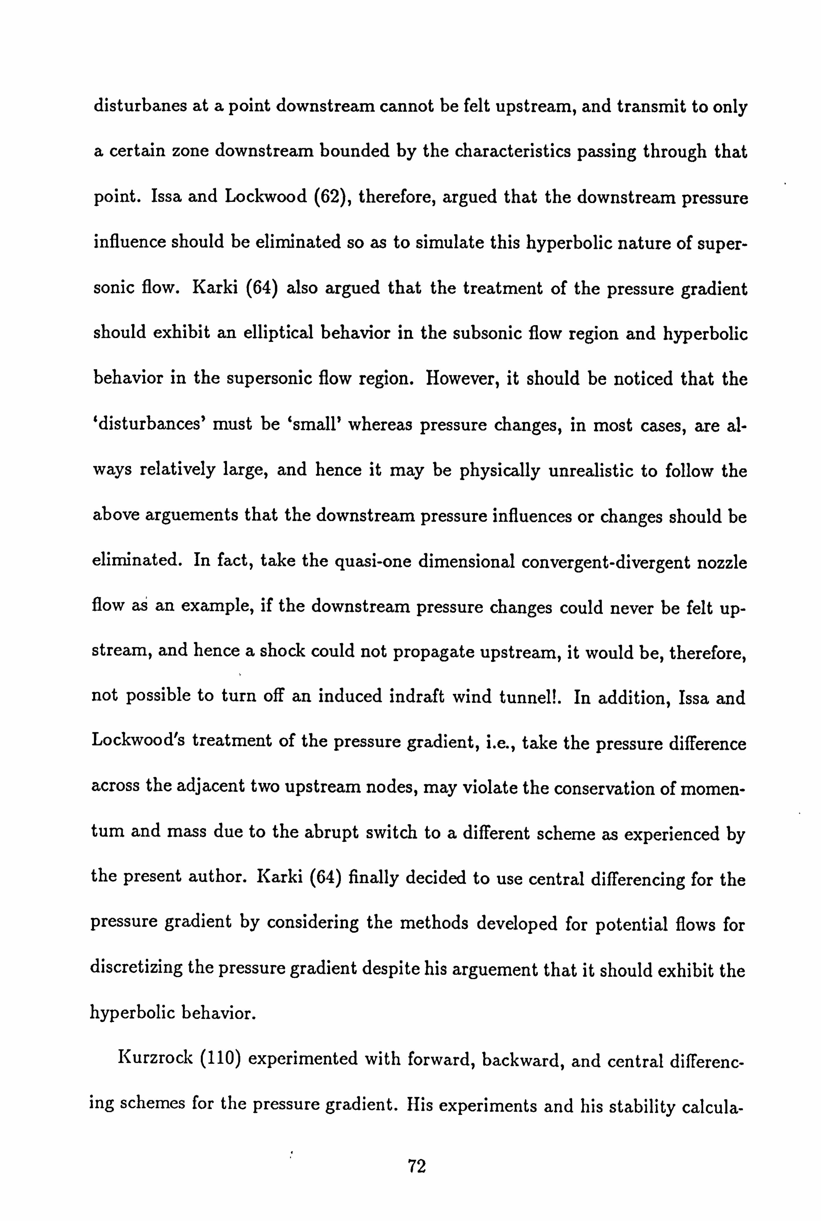
disturbanes at a point downstream cannot be felt upstream, and transmit to only
a certain zone downstream bounded by the characteristics passing through that
point. Issa and Lockwood (62), therefore, argued that the downstream pressure
influence should be eliminated so as to simulate this hyperbolic nature of super-
sonic flow. Karki (64) also argued that the treatment of the pressure gradient
should exhibit an elliptical behavior in the subsonic flow region and hyperbolic
behavior in the supersonic flow region. However, it should be noticed that the
`disturbances' must be `small' whereas pressure changes, in most cases, are al-
ways relatively large, and hence it may be physically unrealistic to follow the
above arguements that the downstream pressure influences or changes should be
eliminated. In fact, take the quasi-one dimensional convergent-divergent nozzle
flow as an example, if the downstream pressure changes could never be felt up-
stream, and hence a shock could not propagate upstream, it would be, therefore,
not possible to turn off an induced indraft wind tunnel!. In addition, Issa and
Lockwood's treatment of the pressure gradient, i. e., take the pressure difference
across the adjacent two upstream nodes, may violate the conservation of momen-
turn and mass due to the abrupt switch to a different scheme as experienced by
the present author. Karki (64) finally decided to use central differencing for the
pressure gradient by considering the methods developed for potential flows for
discretizing the pressure gradient despite his arguement that it should exhibit the
hyperbolic behavior.
Kurzrock (110) experimented with forward, backward, and central differenc-
ing schemes for the pressure gradient. His experiments and his stability calcula-
72

tions show that the central differencing scheme is perferable. Moreover, almost
all the unsteady methods developed for compressible flow (26,27,33,37,53) em-
ploy the same differencing scheme for the pressure gradient no matter whether
supersonic or subsonic flow is calculated.
Due to all the reasons and facts presented above the present modified solution
procedure uses the central differencing scheme for the pressure gradient in both
supersonic and subsonic flow regions. It has been found that this practise has
given good performance for several supersonic flow cases. It is worth pointing out
that the specification of the computational boundary conditions is more crucial
in compressible flow calculations, especially in supersonic flow calculations as the
established principle is misleading as pointed out above, this will be discussed in
more detail in chapter six.
4.4.4 The Pressure-Correction Equation
The pressure-correction equation is derived from the momentum and continuity
equations by assuming that the current velocities calculated using the guessed
pressure field will not satisfy the continuity equation, and hence there must be
an adjustment or a change to the pressure field. As a result of this, velocities
will change correspondingly as expressed in Eq. (4.8) and Eq. (4.9). However,
when compressible flow is under consideration density will also change due to the
pressure change which can be expressed as follows:
p= p* + p' (4.27)
73

the density change p' is related to the pressure change through the equation of
state, and can be expressed in the following form:
P, = KP' (4.28)
where K can be evaluated from the equation of state as follows:
P (4.29) P RT
K= äP RT
(4.30)
where R is the gas constant and T is temperature.
The finite difference form of the continuity equation in the two dimensional
case is:
(pU)e - (pU)w + (PV). - (pV)a =0 (4.31)
When the pressure field changes the velocity and density fields will also change.
The mass flux, e. g., (pU), can be evaluated as follows:
(PU)e = (P* + P)e(U* + U')e (4.32)
expanding the above equation, one has:
ýPU)e = (P*U*)e + (P*U, )e + (P, U*)e + Wu I )e (4.33)
The fourth term on the right hand side of the above equation is one order smaller
and hence can be neglected. The above equation then reduces to the following
form:
(pU)e = (p*U*)e + (p*U')e + (p'U*) (4.34)
74

As the central differencing scheme is still used for the pressure gradient, Eq. (4.14)
and Eq. (4.28) are then substituted into the above equation to yield the following
equation:
(pU). = (p*U*)e + (p*D°)e(P' - PP) + (U*KP')e (4.35)
(pU),,,, (pV),,, (pV), can be also obtained in the same way and expressed as
follows:
(pU)w = (p*U*)
w+ (p*DU)w(P1',
- Pp) + (U*KP')w (4.36)
(pV )n = (p*V *)n, + (p*DV)n(PP - Pk) + (V*KP')n (4.37)
(pV)3 = (p*V*) + (p`DT')3(PP - Pp) + (V*KP)i (4.38)
When the upwind differencing scheme is used the values of density correction
at the control volume boundaries, taking e as an example, can be evaluated as
follows:
p'Pmax[U, *, 0.0] + p'' max[-Uß, 0.0] (4.39)
substituting these relations into Eq. (4.32) and after some manipulation, the mod-
ified pressure-correction equation is:
aPPP = awPW + aEPE + aNPN + asPP + So (4.40)
aw = Avy(pwDw + Kwmax[U,, 0.0]) (4.41)
aE = Au E(p, DE + KEmax[-Uß, 0.0]) (4.42)
aN = AN(p*Dvi + KNmax[-U, , 0.0]) (4.43)
as = AS(p; Ds +Ifsmax[U,, 0.0]) (4.44)
75

ap =A y(pwD°y + Kpmax[-Uu , 0.0]) + AE(p: DE + Ifpmax[UU, 0.0])
+AN(pnDN + Ifpmax[U, , 0.0]) + AS (p, 'DS + KPmax[-U;, O. 0]) (4.45)
So = Aw(P`U'),,, - AE(P"U`)e + As (P`V *)" - AN(P*V*)n (4.46)
Karki (64), however, employed the above modified pressure-correction equation
to update only the velocity field whereas the pressure field was corrected by an-
other pressure-correction equation which he termed the `first' pressure-correction
equation. This so called `first' was also derived from the momentum and conti-
nuity equations in more or less the same way as the derivation in SIMPLER (7,
19). It differs from the above pressure-correction equation in that the full mo-
mentum equations were used, i. e., the two terms Ea�bU, 6, EanbVfb in Eq(4.12)
and Eq. (4.13) were not neglected in the derivation. Details can be found in (64).
However, it has been experienced by the present author that the above modi-
fied pressure-correction equation (4.42) does not show any superiority to the un-
modified one. In principle, density changes should be accounted for in deriving
the pressure-correction equation in the case of compressible flow. Nevertheless,
the density field is renewed once a new pressure field is obtained, which means
that density changes will be accounted for after one iteration. In other words,
density changes lag behind one iteration in the case of compressible flow when
the unmodified pressure-correction equation is used. It is worth pointing out that
this treatment of density is exactly the same way in which the non-linearities of
the momentum equations are treated. Therefore, the original pressure-correction
equation is employed in the present study, and the results obtained confirm that
76

it did lead to a convergent solution for compressible flow provided the calculation
of density was switched on after a reasonable pressure field had been established
and the computational boundary conditions were specified properly.
4.4.5 Summary of the Solution Procedure
In this chapter, a brief introduction was given to the derivation of the finite dif-
ference equations from the corresponding governing partial differential equations,
the solution of these equations and so on. Detailed discussion was presented about
the evaluation of density at the control volume boundaries and the differencing
scheme for the pressure gradient in the case of supersonic flow. It was clearly
stated that the idea to completely eliminate downstream pressure influence to
simulate the hyperbolic nature of supersonic flow sounded correct superficially
but actually was misleading. The pressure-correction equation was also discussed
in more detail with the conclusion that the pressure-correction equation did not
need to be modified necessarily for compressible flow. The overall solution pro-
cedure is as follows:
1). The initial values of the flow field variables are specified or simply set
equal to zero.
2). The momentum equations are solved using the currently available pressure
field.
3). The pressure-correction equation is solved and the pressure and velocity
fields are updated.
4). The transport equation of the stagnation enthalpy is solved to get tem-
77

perature.
5). The calculation of density is switched on after a reasonable pressure field
is established, that is after a certain number of iterations if compressible flow is
under study.
6). Other transport equations are solved if necessary.
7). A new iteration is then started until a fully convergent solution is reached.
78

Chapter 5
APPLICATIONS TO
STRONGLY SWIRLING
FLOWS
In this chapter, the prediction procedure is applied to strongly swirling con-
fined incompressible turbulent flows in vortex throttles. As stated in previous
chapters there is usually no difficulty in obtaining a good numerical solution for
incompressible flows, and the SIMPLE algorithm incorporated in the prediction
procedure has been well tested for incompressible flows (13,14,15,16,17,18).
However, turbulence modelling is still a challenge in the case of strongly swirling
turbulent flows. It is expected that for strongly swirling flows, the anistropy
becomes more and more important, resulting in the components of turbulent vis-
cosity, µ,. x, µe etc. adopting different values (95,96). The conventional two
equation k-c model uses the same value for all the components of turbulent vis-
79

cosity according to the Boussinesq assumption, which is appropriate for isotropic
turbulent flows. It is generally accepted that Reynolds stress models, predict-
ing each component of the Reynolds stresses separately, offer more universality
but they have not been thoroughly tested for recirculating, swirling flows etc.
An attempt is made in the present study to employ a Reynolds stress model
and compare the performance of such a Reynolds stress model with that of the
two equation k-e model in the case of strongly swirling confined turbulent flows.
In addition, a conventional wall treatment (97) and a modified wall treatment,
based on Chieng-Launder (98) and Johnson-Launder -wall treatment (97), are
employed in order to model the near wall region more carefully, and their relative
performance compared. In all cases the results are compared with experimental
data.
5.1 Introduction
Swirling flows are very important phenomena found in nature and they have
become of interest in association with a wide range of applications. In nonreac-
tive cases applications include, for example: vortex amplifiers, cyclone separators,
agricultural spraying machines, heat exchangers etc. In combustion systems, such
as in gasoline engines, gas turbines, industrial furnaces, the dramatic effects of
swirl to stabilize flames and to improve combustion efficiency have been known
and appreciated for many years. Better understanding of swirling flows will un-
doubtedly help the improved design of the various devices and bring about more
80

new applications. However, the strongly coupled, nonlinear governing partial
differential equations and the complex nature of turbulence impose formidable
difficulty to solution by analytical methods. An alternative approach is the nu-
merical solution procedure.
For the strongly swirling incompressible turbulent flow computations, the
most difficult problem to deal with is the turbulence modelling. The conventional
two equation k-e model has been well tested and successfully applied to numerous
engineering calculations but its performance becomes poor for certain situations
such as recirculating and swirling flows, especially for strongly swirling flows (4,
17,96,99,100). This may be attributed to the assumption of isotropic turbulence
which is not appropriate for swirling flows as anisotropy becomes more and more
important. Experimental study of swirling flow (101), free swirling jets (102) and
the flow field near the recirculation zone at the exit of a swirl generator (103)
have shown that the axial and radial components of turbulent viscosity change
significantly, yielding a considerable degree of anisotropy. Modifications could be
made to account for the anisotropy by specifying the r9-viscosity number etc.,
a,. 8 = 1, which is in general larger than 1 (96). However, since this is too
empirical and flow dependent it can be hardly accepted in terms of universality.
Boysan and Swithenbank (17) applied an algebraic stress model to the prediction
of strongly swirling confined turbulent flow in a cyclone chamber and showed that
some important flow features could be captured using the algebraic stress model
whereas the two equation k-e model failed to reproduce them. An evaluation of
the performance of the two equation k-e model and algebraic stress models was
81

presented by Nallasamy (4), concluding that the performance of the conventional
two equation k-e model becomes poor for attached flow, recirculating flow, swirl
flow etc. and algebraic stress models perform better. It is also pointed out by
him that Reynolds stress models have not been thoroughly tested for recirculating
and swirling flows.
In this chapter, calculations have been performed for strongly swirling con-
fined turbulent incompressible flows in 76mm and 102mm chamber diameter vor-
tex throttles. Both the widely tested conventional k-e model and a Reynolds stress
model are employed in the study for the sake of comparison. Wall functions are
used to simplify the calculations in the near wall region, and both a conventional
wall treatment (97) and a modified wall treatment, based on Ching-Launder (98)
and Johnson-Launder wall treatment (97), are adopted. The predicted pressure
drops through the vortex throttles over a certain range of flow rate are compared
with experimental data. The predicted streamlines, velocity profiles etc. are
presented and the flow field structure is analyzed. Moreover, numerical exper-
iments have been made to assess the effect of inlet swirl intensity (the ratio of
inlet tangential velocity to inlet radial velocity), the inlet Reynolds number, and
inlet turbulent intensity on the flow fields. Finally, further exploration of pressure
drop in such vortex throttles is given and some other possible applications are
discussed.
82
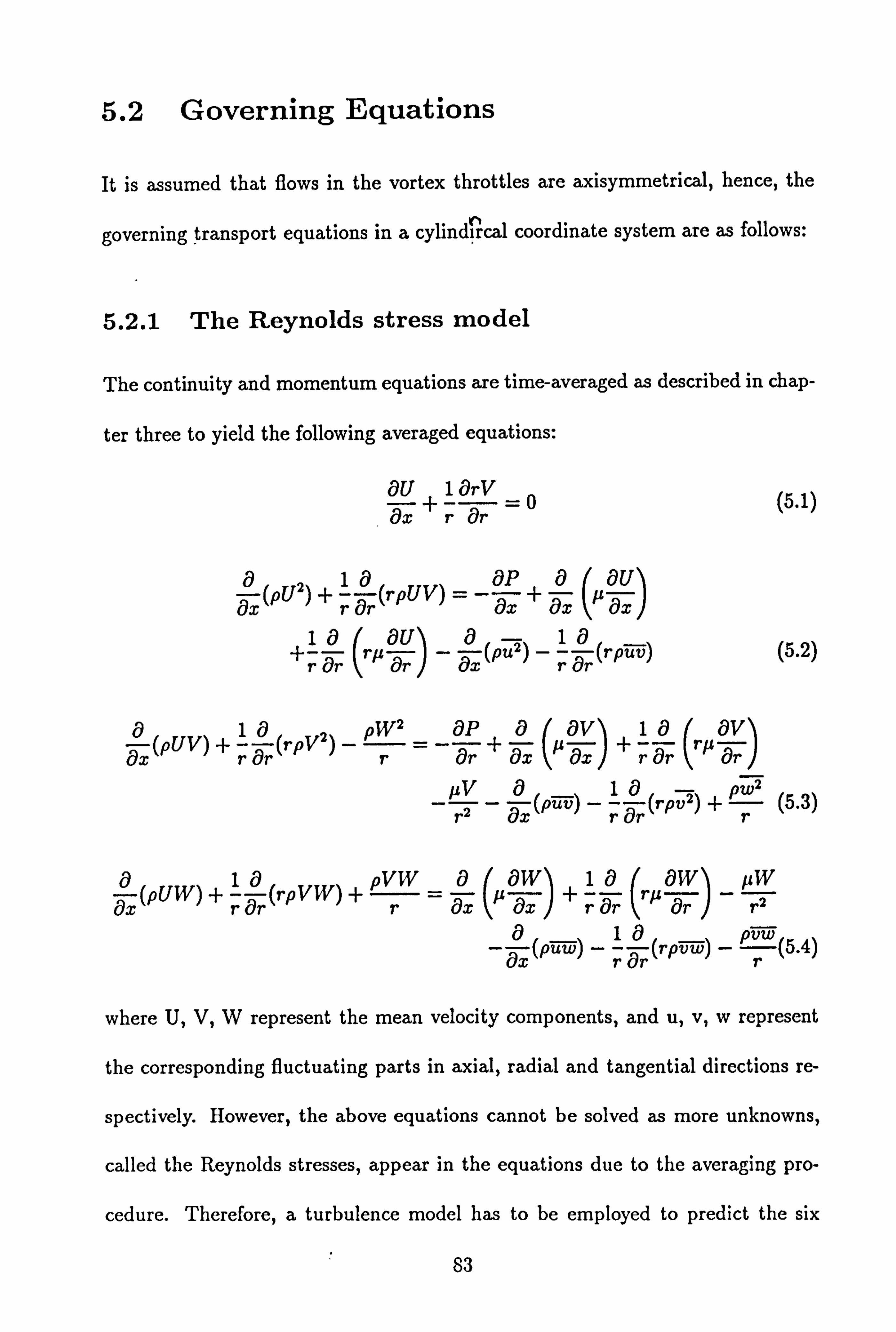
5.2 Governing Equations
It is assumed that flows in the vortex throttles are axisymmetrical, hence, the
governing transport equations in a cylind rcal coordinate system are as follows:
5.2.1 The Reynolds stress model
The continuity and momentum equations are time-averaged as described in chap-
ter three to yield the following averaged equations:
äU +
lärV (5.1) äx r Or
a21a aP a(aul ax
(pu) +r ar (r pUV) =- ax + ax p ax
+r 37 (rý a_)
-5 (put) -r- (rpüv) (5.2)
a1a 2) pW2 = _aP
a( aaxyl 1ra( ayl ax
(pUV) +r Or (rPV
r ar+ axJ+ Tr `rp Or
_z -
r2 - (püv) -r- (rpv2) + pr (5.3)
as ax
(pUW) + rar
(rpVW) + pVW raax
(paWax) +r aa r
(rlz"W) W 8r r2
-x(püw) - (rpvw) - prw(5.4)
where U, V, W represent the mean velocity components, and u, v, w represent
the corresponding fluctuating parts in axial, radial and tangential directions re-
spectively. However, the above equations cannot be solved as more unknowns,
called the Reynolds stresses, appear in the equations due to the averaging pro-
cedure. Therefore, a turbulence model has to be employed to predict the six
83

Reynolds stresses directly or indirectly. In the Reynolds stress model employed
in this study, the modelled transport equations for k, v2- - u2-, v2 - w2, üv, üw,
vw and c are as follows:
frk)+ 1 rvk) . (v + r) + rar ax ax rar är,
(au av au av v aw aw w ax + vw r (5.5) -üv ä7r + ax) - u2 ax -
v2 är - w2 r- VW-Ur- - uw-
F [U(; )2
- u2)] + Tar
[rV (v2 -
u2)] - 2vw
W= qx (v + r) av
ax u
uZ)l - 2Z
(v2 - u2) -
Cl (v2 - u2) +r
ar r(v + r) a(v
Or J
-2(1 - a) Luv (9v
-auf + v2- -z
aU - VU-11] (5.6)
äý Or J Or ax r
[U(v2 - w2)ý ý"
r är [rV (v2
- w2)ý - 4vw W=
(v + r) av
ax
w (2- 2']
2) _ 1 t9- +T
Fr(v+r)0'' a(72 ar
42 (i - w2)
- Cl k (v2 - w2)
- w2 -w ýW
-} W-w ýWl
(5.7) -2(1 - a) IUV ýx
-} v2 ýV
Tr r Cý J
0 49 ax(Uüv) -I-
r
r(rVü) - üwW =x [(v
+ r) ä- +
rär
[r(v+r)
är
j-
zr uv-Clkuv-
u av au av) (1 a)
ýV2_F + u2 ax + uv
(äx + är- - uwWl (5.8)
J
äx (Uüw) +rr (rV uw) + üv =
[(v + r) 1+r ex ex
- [r(U
+ r) ar - r2 ü- Cl ü-
r är
(1 - a) [F
wau + ii w au äx +
r) +v
ýý + u2
ex (5.9)
84
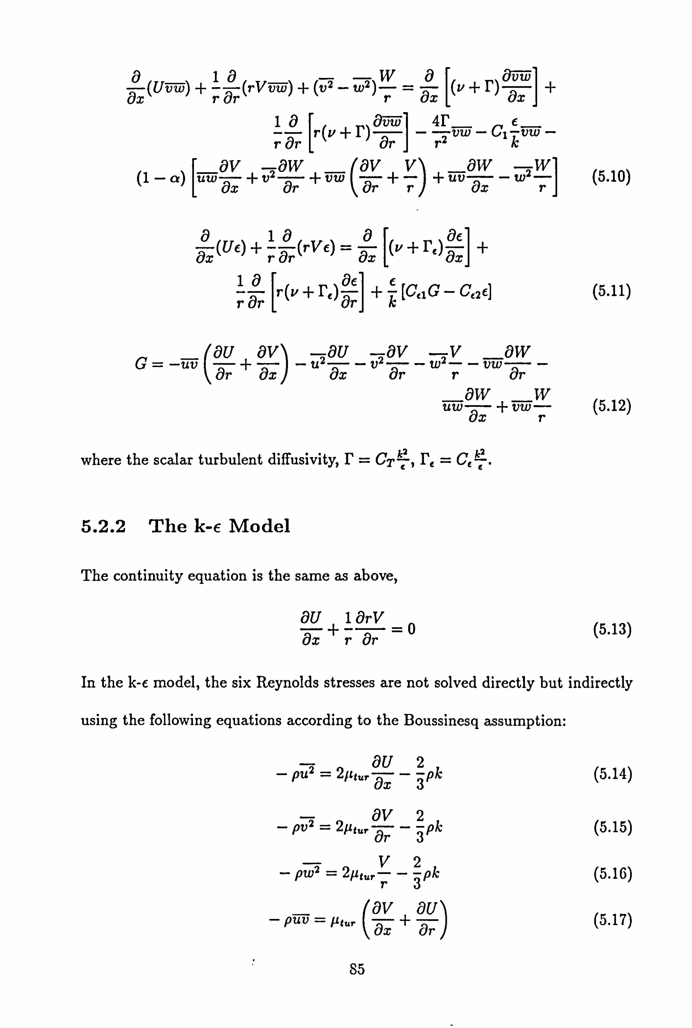
TX (Uvw) +r (rV vw) -}- (v2 - w2) W=T [(v+r)j+
5r- r rar
[r(v+r) or J- rZvw-CIkvw-
(1-a) Iiiw +v2as -} vw(ýv+ T
+iii aW
7x -wýWJ (5.10)
TX (v6) +1ä (rvE) =ä [(v+r)] +
1 2- [r(v + r, ) ac +k [CE1G - Ce2e] (5.11)
rýr
]
(är au av) av av v aw G= -üv + ax J- u2 ax - v2 er -wzr - vw ar -
uw ýw
+vW (5.12) xr
where the scalar turbulent diffusivity, I' = CT7, r= CE E'.
5.2.2 The k-c Model
The continuity equation is the same as above,
äU 1 örV öx r ar
0 (5.13)
In the k-e model, the six Reynolds stresses are not solved directly but indirectly
using the following equations according to the Boussinesq assumption:
- Put = ZEttur 5x
-3 Pk 5.14)
- pv2 = 2µe, ir ý7
-2 pk (5.15)
-pwz=2pt, r
-2pk (5.16)
pü =I tur Cav + avl (5.17) Tx or
,
85

aW 5.18 p7121J - /tur ax
(äw - W) (5.19) - pw = µeur är rJ
Substituting the above relations into the averaged momentum equations and
after some manipulations the momentum equations have the following forms:
a (pU2 1a aP a( aU) 1 a( aUl (5 äx
)+r Or
(r pUV) =- äx + äx `1L`! i äx) +r
är `rýCýf fr J (5.20)
a (pUV) +ia (rpvz) _ Pw2 = _a- +a jeffav + TX rar r Or ax ax
1a av) lirffV (5.21) rar
rpýff ar r2
a1a pyW ar aW 1
aý(pUW) +r ar(rpVW) +_
r a. (JLeff
ax )
+1 a (rp,,
ff aw)
- P°ffW (5.22)
r Tr ar r2
where U, V, W represent the mean velocity components in axial, radial and tan-
gential directions respectively. µeff is the effective viscosity expressed as follows:
ILeff =P+ Pour (5.23)
where pt, is the turbulent viscosity which is obtained from the following equation
2 µtur = Cup
kf (5.24)
and the transport equations for k and e are as follows:
aaa /LtuTl ak TX (pUk) +r ar (rpV k) = ax
Cµ + Prk J ax)
+r Or
[r (jz + pt., )
I ar] + Gk - PC (5.25) k
86

I-(pU) aa ýturl aE 1 +rar(rpVE)= ax [Cý+
Pr: )
ax1 +
1a '96 f r Tr
[r (11 + Pfit ry J ar, + k(C`lGk - C`2PE) (5.26)
au2 av2 (vl2 Gk = 2fýeur (ax)
+ (ar)
+\r/+
222
11tu (aU + aý + axý + [rar (--)j I(5.27)
The numerical constants used in the above equations take the following values
in both models:
Cµ Cl CT a Prk Pr, CE Cpl CE2
0.09 1.5 0.1 0.4 1.0 1.3 0.07 1.44 1.92
5.3 Wall Treatment
For wall-bounded flows, a special treatment should be employed to handle a region
near the wall where viscous effects become important and the turbulence levels
decrease. There are usually two ways by which one can achieve this, i. e., either
using low Reynolds number turbulence models or using wall functions. The latter
approach is adopted in this study and more details about the wall treatment is
given elsewhere (97). Here an outline is presented.
5.3.1 The Conventional Wall Treatment
The expression for the wall shear stress given in (97) is as follows:
0 , UP C, i 141c 2
Tw = (5.28)
In Ey+
87

where subscript P refers to values at a point P in the inertial sub-layer and E
is a constant, x is the von Karman constant. The values of these two constants
are determined from the experimental logarithmic law as, rc = 0.4187, E=9.793.
yk1/2 C, 1/4
Y=P &I ,y is the distance from the wall and v is the kinematic viscosity.
Cµ is a constant whose value is 0.09. It is assumed that the shear stress in the
viscous sub-layer is constant and equal to that of the inertial sub-layer. Therefore,
the shear stress in both the viscous and inertial sub-layer is the same as that of
the wall shear stress which is then used in the momentum equations in the wall-
adjacent grid cells.
The same needs to be done in the wall-adjacent grid cells for k and e. For
k, the generation and dissipation rates must be specified. The generation rate is
assumed to be
T +dW/ -Tw UP-0+Wp-0
_Tr(UP+WP) (5.29) w
(dUTY dy \yP-0 yP-0 yP
The dissipation rate for both k and c is assumed to be
k3/2
e= CtyP (5.30)
where Cl is a constant defined as
Cl =C /4 (5.31)
This conventional wall treatment has been used traditionally by the Imperial
college group and hence is denoted as the IC wall treatment in (97).
88
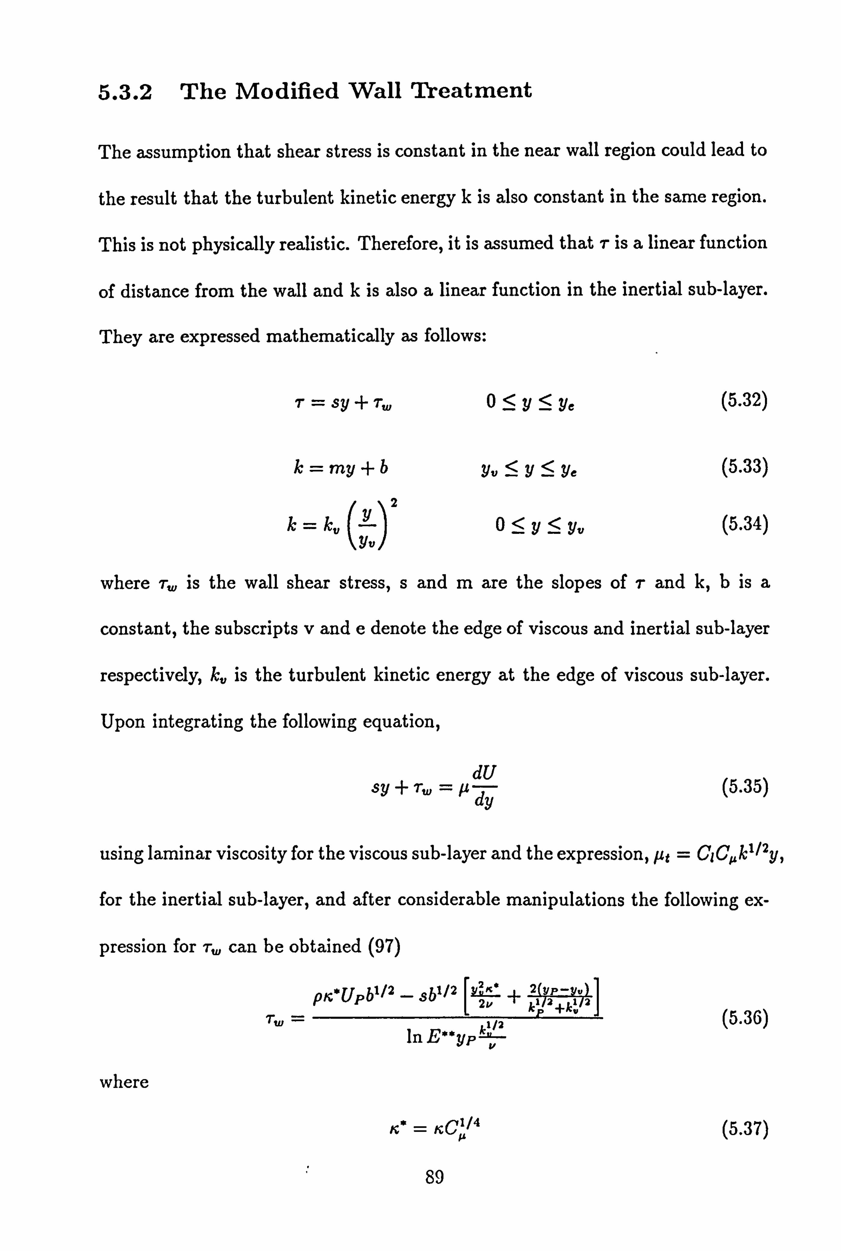
5.3.2 The Modified Wall Treatment
The assumption that shear stress is constant in the near wall region could lead to
the result that the turbulent kinetic energy k is also constant in the same region.
This is not physically realistic. Therefore, it is assumed that r is a linear function
of distance from the wall and k is also a linear function in the inertial sub-layer.
They are expressed mathematically as follows:
T= Sy + Tw 0SY: 5 Ye (5.32)
k=my+b y�<y<ye (5.33)
/ k=k�i y)z 0< y_ y� (5.34)
yv
where Tw is the wall shear stress, s and m are the slopes of r and k, b is a
constant, the subscripts v and e denote the edge of viscous and inertial sub-layer
respectively, k� is the turbulent kinetic energy at the edge of viscous sub-layer.
Upon integrating the following equation,
dU sy + Tw = it (5.35)
using laminar viscosity for the viscous sub-layer and the expression, µt = C1Cµkll2y,
for the inertial sub-layer, and after considerable manipulations the following ex-
pression for Tw can be obtained (97)
pfe*Upb' - sb112 I
ý2 + 21 2' lV 2
_k +k�
Tw 1n E**
#P k-"/
P (5.3G) v
where
r Cµ14 (5.37)
89
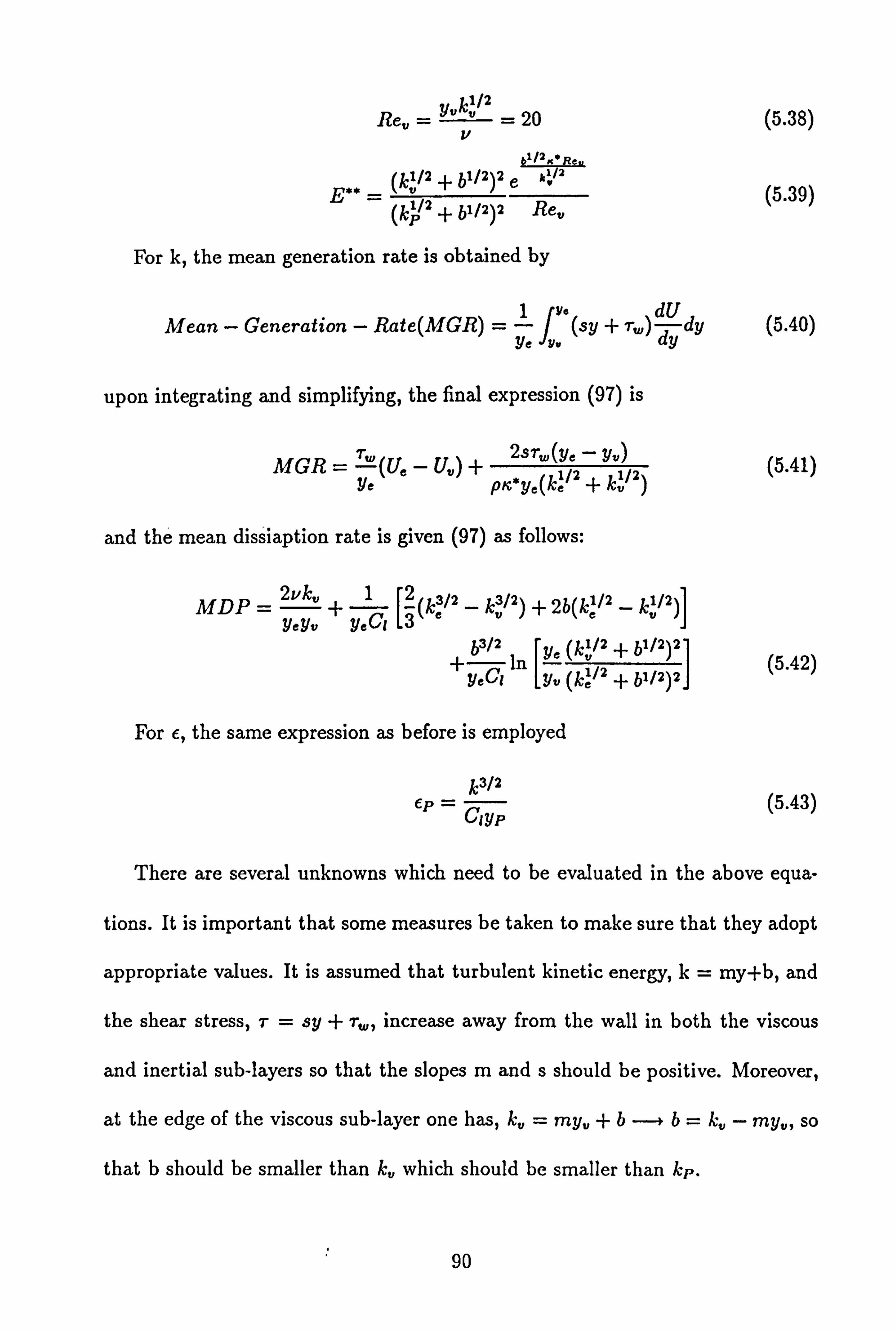
=v °/2 Re� yk = 20 (5.38)
v 61/2 *Re
E** . (k"/2 + bl/2)2 e kj 2 k' 2+ bl/2)2 Re�
(5.39)
For k, the mean generation rate is obtained by
Mean - Generation - Rate(MGR) =1-f ye(sy +Tw)
dU d dy (5.40)
Ye Y. y
upon integrating and simplifying, the final expression (97) is
MGR = Tw M- U�) +
2srw(y Z-
y ýý (5.41)
Ye P, c`Je(ke + kv
and the mean dissiaption rate is given (97) as follows:
MDP = 2ykv
+ [k/2
- k/2) -I- 2b(k/2 - k/2)] yeyv ye Cl 3
b3/2 [(kl/2 + b1/2)21 +Y C1
in yv (ke/2 + bl/2)2 J (5.42)
For c, the same expression as before is employed
k3/2 ep Cjyp (5.43)
There are several unknowns which need to be evaluated in the above equa-
tions. It is important that some measures be taken to make sure that they adopt
appropriate values. It is assumed that turbulent kinetic energy, k= my+b, and
the shear stress, T= sy +, r,,,,, increase away from the wall in both the viscous
and inertial sub-layers so that the slopes m and s should be positive. Moreover,
at the edge of the viscous sub-layer one has, k,, = my,, +b -º b= k� - my,,, so
that b should be smaller than k� which should be smaller than kp.
90

5.4 Boundary Conditions
The treatment of the boundary conditions for incompressible flows is well docu-
mented in (2). The boundary conditions used in this study are given briefly as
follows:
5.4.1 Inlet Boundary
The values of the variables are usually known or can be calculated from the given
conditions at the inlet boundary. The values are used in the boundary control
volumes in the discretization equations and nothing special requires to be done.
One point which should be noted is that a boundary condition for pressure is not
required due to the use of staggered grids. Therefore, in the present work only
the velocities were specified at the inlet boundary.
5.4.2 Outlet Boundary
The fluid leaves the computational domain at the outlet boundary and usually
there is no information about the variables. This boundary is often an artificial
boundary used to limit the computational domain to a finite region. Hence, the
outlet boundary should placed and treated such that it minimizes the influences
on the results in the region of interest. In this study, the tangential and radial
velocity component gradients were assumed to be zero and the axial velocity
component was adjusted to satisfy overall mass conservation.
91

5.4.3 Wall Boundary and Symmetry Line
At the solid wall, the no-slip condition is usually applied for viscous flows. Ac-
cording to this condition the velocity of the fluid at the wall should be the same
as that of the wall. In the study, all the walls are fixed and hence the velocities
at the wall were zero. At a symmetry line, the normal component of velocity and
the normal gradient of the parallel component of velocity are zero. In this case at
the axis of the symmetry, the tangential and radial velocities, W and V, vanish
under the assumption of axi-symmetric flow.
5.5 Geometry of Vortex Throttles
Figure 5.1 shows the geometry of vortex throttles used in this study. They are of
the square-edged type with symmetrical structure. Flow enters at the tangential
port, forms a vortex in the chamber and leaves through the axial port. The
following table gives details of the value of the various dimensions in millimeters,
as defined in Figure 5.1.
D h w da 1s Dp D;
102 13.12 10.05 12.75 12.95 14 38 19
76 13.12 10.20 12.85 13.05 13 38 19
The inlet tangential and radial velocities are calculated from the given flow
rate and Reynolds number.
92

5.6 Results and Comparisons
Fig. 5.2 and Fig. 5.3 compare measured and predicted pressure drops with the
two equation k-c model for various water flowrates through both the 76mm and
102mm chamber diameter vortex throttles respectively. It can be seen that bet-
ter agreement has been achieved between the experimental data and the results
predicted using the modified wall treatment, compared with the relatively poor
predictions obtained using the conventional wall treatment. This confirms that it
is important to handle the near wall region carefully since the conventional two
equation k-e model and some of the other turbulence models are appropriate to
high Reynolds number flows only. This also indicates that the wall shear stresses
play a important role in determining the pressure drop in the vortex throttles
as will be discussed below. All predictions presented hereafter are obtained with
the modified wall treatment.
Fig. 5.4 shows experimental data and the two equation predictions of pressure
drop versus the flowrates through both the 76mm and 102mm chamber diameter
vortex throttles. It can be seen that measured pressure drops across the 76mm
diameter vortex throttle are slightly larger than those of the 102mm diameter
one. This again indicates the importance of internal wall friction (wall shear
stresses) in determining the pressure drop as mentioned before. In the absence of
internal wall friction, the strength of the potential vortex in the vortex chamber
would increase with increasing chamber diameter. In practice, however, internal
wall friction forces limit this effect. It can also be seen from this figure that the
93
two equation k-e model fails to predict the higher pressure drop as measured in
the 76mm chamber diameter vortex throttle.
Fig. 5.5 compares the Reynolds stress model predictions of pressure drops
with experimental data in both the 76mm and 102mm chamber diameter vortex
throttles. It can be seen that the Reynolds stress model predictions give not
only closer agreement with the experimental data but also slightly higher pres-
sure drops in the 76mm chamber diameter vortex throttle. This verifies that
the Reynolds stress model offers more universality and gives better predictions
than the two equation k-e model in the case of highly swirling flows despite its
complication and requiring more CPU time.
Fig. 5.6 shows the ideal free vortex tangential velocity profile and the pre-
dicted profiles for Re=11078 in the 102mm chamber diameter vortex throttle at
x/R=0.065. For a free vortex the tangential velocity can be expressed as Wr=C,
where C is a constant and r is the distance from the axis. Hence the tangential
velocity goes to infinity at the axis in the case of a free vortex. In reality, how-
ever, the tangential velocity is zero at the axis of symmetry and has the Rankine
free-forced vortex form in the vortex chamber as shown. It can also be seen that
the peak value of the tangential velocity predicted by the Reynolds stress model
is larger than that predicted by the k-e model, which agrees with the higher
pressure drop predicted by the Reynolds stress model as will be discussed later.
Fig. 5.7 shows the experimental and predicted data plotted as Euler number
versus Reynolds number for the 102mm throttle, based on the the flow condition
at the inlet tangential port. The Reynolds stress model predictions are again
94
closer to the experimental data than the k-e model predictions. It can be also
seen that the performance of the throttle is a strong function of Reynolds number
below about Re=10,000, with Euler number rising from a minimum value of
about 10 to a maximun value of about 60. However, when Reynolds number is
over 10,000 Euler number is seen to be fairly constant at the maximum value.
Fig. 5.9 and Fig. 5.10 compare the Reynolds stress model and k-e model
predictions of tangential and axial velocity profiles for the 102mm throttle at
Re=11078. Fig. 5.9 shows that the Reynolds stress model predicts a sharper
tangential velocity profile in the vortex chamber, as can also be seen from Fig.
5.6. By comparison, the two equation k-e model predicts a flatter and smoother
tangential velocity profile. This may be attributed to the overprediction of the
turbulent kinetic energy by the k-e model, as can be seen in Fig. 5.8 which
shows turbulent kinetic energy predicted by the Reynolds stress model and the
k-e model resprectively for Re=11078 in the 102mm diameter vortex chamber at
x/R=0.065. Near the axis the Reynolds stress model predicts a lower tangential
velocity compared with the k-e model. This may be because the Reynolds stress
model predicts a stronger recirculation region along the axis, bringing more fluid
with very low tangential velocity back, which can be seen from the axial profiles
as shown.
Fig. 5.11 shows streamlines in the 102mm chamber diameter vortex throttle
obtained by the Reynolds stress model and the k-e model at Re=11078. Some
differences can be observed between the Reynolds stress model predictions and
the k-c model predictions, especially in the vortex chamber where slightly differ-
95

ent flow patterns have been predictied. This is probably due to the difference
of tangential velocity predicted by the two models. Higher tangential velocity is
predicted by the Reynolds stress model in the chamber near the axial port, re-
sulting in higher centrifugal force which causes more outward radial flows, hence
a strong recirculation zone is predicted in the vortex chamber. The recirculation
zone is also predicted, though to a lesser extent, by the two equation k-e model.
At the axial port exit the flow patterns predicted by both the Reynolds stress
model and the k-e model are very similar and a recirculation zone which is usually
referred to as CTRZ (Central Toroidal Recirculation Zone) is predicted by both
models. Details of the flow structure will be discussed in the next section.
The results for the 76mm diameter vortex throttle are almost the same as
those for the 102mm diameter one so that it is not necessary to present them
again. They are not presented in the following discussion for the same reason.
5.7 Discussions of the Results
It has been well established that swirl flows can be classified into two groups
according to the degree of swirl strength. They are the low swirl and high swirl
flows respectively, and the flow characteristics are quite different in the two cases.
The degree of swirl is usually characterized by the so called swirl number S,
which stands for the ratio of axial flux of swirl momentum to axial flux of axial
momentum (96). At higher degrees of swirl (S is larger than 0.6), strong radial
and axial pressure gradients are set up, resulting in axial recirculation in the
96

form of a CTRZ (Central Toroidal Recirculation Zone) as metioned above. The
study undertaken belongs to the high swirl flows, and one point which needs to
be noted is that the inlet swirl intensity (the ratio of inlet tangential velocity to
inlet radial velocity) is used to characterize the flow field for convenience instead
of swirl number S in the present study.
5.7.1 Pressure Field
Fig. 5.12 shows the pressure profiles and the pressure contours predicted by the
Reynolds stress model in the 102mm diameter throttle at Re=11078. The radial
pressure gradient in the vortex chamber near the axis is apparent (as can be seen
from both the profile and contours) and the axial pressure gradient can be seen
clearly along the axis. From the pressure profile in the vortex chamber one can
see that a low pressure zone occurs around the axis in the vortex chamber as a
result of the centrifugal force. This is the cause of the axial pressure gradient
which results in the axial recirculation. Out of the axial port, pressure is almost
constant due to the decay of tangential velocity. In the vortex chamber the total
pressure, PO WW =P+ 2ý (radial and axial velocities are negligible), is almost
constant. However, out of the axial port both tangential velocity and pressure
are very low, as shown in Fig. 5.9 and Fig. 5.12, which means that a large amount
of total pressure (energy) is lost through the axial port due to wall friction and
the sudden expansion at the exit of the axial port. This indicates the importance
of the design of the axial port and the expansion part in determining throttle
performance.
97

5.7.2 Flow Field
Fig. 5.13 shows the k-c prediction of streamlines and velocity vectors in the
102mm diameter throttle at Re=5565. The salient features of the flow field pre-
dicted are the two recirculation zones, one is in the vortex chamber and another
is along the axis and is referred to as the CTRZ mentioned above, which occurs in
swirl flows when the swirl number is over 0.6. In the particular case under study
it is due to the inlet high swirl intensity (the ratio of inlet tangential velocity
to radial velocity), which creates a large centrifugal force in the vortex chamber,
causing a low pressure zone around the axis as explained above. With respect to
the recirculation zone in the vortex chamber it may be explained as follows:
Because of the viscous action, there is a tangential boundary layer on the walls
in the vortex chamber. In the boundary layer the reduced tangential velocity leads
to a reduced centrifugal force and thus the fluid tends to move inwards as shown in
Fig. 5.13 due to the radial pressure gradient force and the inertial force. Outside
the boundary layer, however, the centrifugal force on a particle of fluid tends to
be balanced by the radial pressure gradient force and the inertial force. When
the inlet swirl intensity increases the tangential velocity rises as well, and so does
the centrifugal force. Eventually a point is reached where the tangential velocity
in the main body of the vortex chamber produces a centrifugal force which just
balances the radial pressure gradient force plus the radial inertial force, this can
be defined as a critical point beyond which the larger centrifugal force will cause
outward radial flow and hence the recirculation zone occurs in the vortex chamber.
However, the chamber recirculation zone is not only dependent on the inlet swirl
98

intensity but also on the inlet Reynold number as well, which will be discussed
later. Moreover, one may notice at the corner region in the vortex chamber near
the axial port where the boundary layer ends, a flow separation can be observed
which is similar to the usual separation in boundary layers. In this particular
case it is because the radial pressure gradient force and the inertial force are not
large enough to maintain inward flow due to an increase of the centrifugal force
just outside the boundary layer. These phenomena are not predicted when the
inlet swirl intensity is small enough as will be discussed later. In addition, when
Reynolds number is changed the flow field also changes which will be discussed
next.
5.7.3 The Effects of Reynolds Number
Fig. 5.14 shows the k-e model predictions of streamlines in the 102mm diameter
throttle at different Reynolds numbers. For all the cases the Central Toroidal Re-
circulation Zone can be clearly seen, and so can the separation zone at the corner
near the axial port in the vortex chamber. In Fig 5.14(a) at Re=3385 and Fig.
5.14(b) at Re=5565 a strong recirculation zone is observed in the vortex chamber.
This is also apparent, though to a lesser extent, in Fig. 5.14(c) at Re=11078.
However, when the inlet Reynolds number is raised to 14600 the reverse flow in
the vortex chamber disappears as shown in Fig. 5.14(d). According to what is
stated above, this means the centrifugal force is no longer larger than the pressure
gradient force plus the radial inertial force. This is probably because the inertial
radial force increases proportionally with the increase of inlet Reynolds number.
99
The centrifugal force rises as well but not so rapidly as the radial inertial force.
In conclusion, the inlet Reynolds number has great effects on the flow pattern in
the vortex chamber but out of the chamber the flow field does not change too
much.
5.7.4 Effect of Inlet Swirl Intensity
It is well known that one of the most important factors influencing a swirling
flow field is the swirl number. In this study, however, the inlet swirl intensity
(denoted hereafter as SI) is adopted for convenience as mentioned before. One
would imagine that the inlet SI will also have great effect on the flow field. All
the results presented above have been obtained when the inlet SI is about 32,
which is the value for the vortex throttles used. For a certain vortex throttle
design the inlet SI is determined solely by the inlet geometry of the throttle. The
results shown below do not refer to any practical vortex throttle and they are
just numerical experiments to assess the effects of the inlet SI on the flow field.
Fig. 5.15 gives the k-e predictions of streamlines in the 102mm throttle at
the same inlet Reynolds number but when the inlet SI is changed. When the
inlet SI is reduced to 15 the flow field does not change too much as can be seen
in Fig. 5.15 (b). By comparison, in the case of low inlet SI, as shown in Fig.
5.15 (c) and Fig. 5.15 (d), dramatic changes occur. The recirculation zone in the
vortex chamber disappears completely and the size of the CTRZ reduces as well.
When the inlet SI is reduced to 1 both the CT1IZ and the separation region at
the corner disappear entirely. This shows that the inlet SI has a great effect on
100

the flow field as does the swirl number, confirming that it is equivalent to use the
inlet SI instead of swirl number to characterize the flow field.
5.7.5 Effect of Inlet Turbulent Intensity
Solving the transport equation for turbulent kinetic energy needs the specification
of the inlet condition, but unfortunately no experimental data is available. In
most cases the inlet turbulent intensity is assumed around 10 to 20 percent. For
the case undertaken 10 percent has been assumed. However, in order to assess
the effect of inlet turbulent intensity several values from 1 percent to 30 percent
have been adopted. It has been found that the change of inlet turbulent intensity
has hardly any influence on pressure drop and mean velocities nor even on the
turbulent kinetic energy and its dissipation rate. This indicates that turbulent
kinetic energy is mainly produced inside the flow field in this case.
5.7.6 Pressure Drop
It would be too broad to discuss pressure drop in general flow fields and it is also
beyond the scope of this thesis. In the following part of the discussion the pressure
drop in the vortex throttles will be discussed, in particular, the important factors
influencing the pressure drop in such a device will be given. Moreover, some
difference between the mechanism causing pressure drop in the swirling flows in
vortex throttles and in pipe flows will be presented.
Pressure drop or pressure loss is actually an energy loss from the point of view
of energy conservation. In the case of swirling flows in vortex throttles, pressure
101

drop (energy loss) occurs mainly through the axial port by dissipating the high
tangential velocity and depends on several factors. This will be discussed as
follows:
In the vortex chamber there is a small amount energy loss due to wall fric-
tion and viscous dissipation although a large pressure gradient exists because of
centrifugal force. The total pressure, Ptotai =P+ 2' (radial and axial velocities
are negligible), is almost constant. However, outside of the axial port both tan-
gential velocity and pressure are very low, as shown in Fig. 5.9 and Fig. 5.12,
which means that a large amount of total pressure (energy) is lost through the
axial port and at the exit of the axial port due to the sudden expansion. This
indicates that higher tangential velocity near the axial port would lead to higher
energy loss as tangential velocity decays very quickly. Therefore, any means to
create a stronger vortex, resulting in higher tangential velocity, would increase
the pressure drop. The ideal case is the free vortex as shown in Fig. 5.6, but
this is impossible in reality due to the viscosity of fluids and wall friction. In nor-
mal pipe flows, increasing wall friction results in higher pressure drop but in the
case under study increasing wall friction in the vortex chamber would reduce the
vortex strength, resulting in lower tangential velocity and hence lower pressure
drop.
Energy is mainly lost through the axial port due to wall friction of the port
and due to the viscous interaction in the fluid because of the sudden expansion at
the outlet of the axial port as well as interaction with the recirculation flow along
the axis. This may be verified by Fig. 5.16 which shows contours of turbulent
102

kinetic energy disspation rate. It can be seen from the contours that turbulent
kinetic energy is mainly dissipated through the axial port. One may infer that
the mean kinetic energy is also largely dissipated through the axial port due to
wall friction of the port and the sudden expansion. This means that pressure
drop across vortex throttles mainly occurs through the axial port. Therefore the
design of the axial port is very crucial, and the wall of the axial port should be
made as rough as possible so as to get higher wall friction. However, the wall
of the vortex chamber should be made as smooth as possible in order to reduce
energy loss in the vortex chamber and hence increase the vortex strength.
The mechanism of turbulence tells us that turbulence extracts energy from the
mean motion by various means such as shear stress, buoyancy and other ways.
Larger eddies formed initially decay into smaller ones until the viscous action
becomes very important and turbulent kinetic energy is then dissipated. This is
essentially irreversible process. Applying this mechanism to the swirling flows in
vortex throttles, it can be concluded that turbulence influences pressure drop by
way of extracting energy from mean motion in the vortex chamber, which reduces
the vortex strength and hence lowers the tangential velocity near the axis. This
is illustrated further by Fig. 5.9 which shows turbulent kinetic energy predicted
by the Reynolds stress model and the k-e model respectively. It can be seen that
much higher turbulent kinetic energy in the chamber has been predicted by the
k-e model, which agrees with a slightly lower pressure drop predicted by the k-e
model as compared with the Reynolds stress model.
In conclusion, increasing any energy loss in the vortex chamber would lead to
103

the reduction of the vortex strength and hence lower tangential velocity, conse-
quently, lower pressure drop. Whereas increasing energy loss through the axial
port and out of it would result in higher pressure drop.
In some applications it would be useful to exploit the high centrifugal force
and tangential velocity created within a vortex, without the penalty of the high
overall pressure loss. This would require recovery of the vortex energy, as opposed
its dissipation in the throttle. Turbulence usually extracts energy from the mean
flow and dissipates it by viscous action, which is against this objective. However,
turbulent kinetic energy is, in most situations, very small compared with the total
kinetic energy and in our case, the Reynolds stress model predictd the turbulent
kinetic energy in the chamber to be only about 3.5%. of the total kinetic energy.
Therefore, Significant energy recovery would be possible if viscous losses due to
the axial recirculation, the sudden expansion of the axial port, and friction losses
within the port, could be minimised.
5.8 Conclusions
Both the widely used two equation k-e model and a more complicated Reynolds
stress model have been employed to simulate numerically the strongly swirling
confined turbulent flows in vortex throttles. The influence of the inlet swirl
intensity, inlet Reynolds number, and inlet turbulence intensity on the flow field
have been analyzed. Several conclusions may be reached.
The wall shear stresses greatly influence the performence of vortex throttles,
104
and careful modelling in the near wall region leads to better results.
The conventional k-E model gives relatively poor predictions compared with
measured pressure drop and fails to predict higher measured pressure drops in a
76mm diameter vortex throttle as compared with a 102mm one.
The Reynolds stress model gives better predictions than the conventional two
equation k-e model for the highly swirling flows, producing good agreement with
measured pressure drop data and successfully predicting the better performance
of the 76mm throttle.
The turbulent kinetic energy predicted by the conventional k-e model in the
vortex chamber is much higher than that predicted by the Reynolds stress model.
This explains why the Reynolds stress model predicts higher pressure drops since
the vortex is stronger if turbulent kinetic energy is lower as discussed before.
The swirl intensity can be equally used as the swirl number to characterize
the flow field in vortex throttles. Numerical experiments showed that the flow
field changed enormously when the inlet swirl intensity reduced, and all the re-
circulating flow in the high inlet swirl intensity disappeared when the inlet swirl
intensity reduced to one.
The inlet Reynolds number influences mainly the flow field in the vortex
chamber. The recirculation zone reduces when the inlet Reynolds number in-
creases and it disappears completely when the inlet Reynolds number is above
approximately 14600 according to the predictions.
The inlet turbulence intensity has little influence on the overall predictions.
This was shown when the inlet turbulence intensity was changed from 1% to 30%
105

since the mean variables hardly changed.
The pressure drop through vortex throttles differs from that in pipe flows due
to the mechanism of swirl conservation. It depends on mainly dissipating the
high tangential velocity created in the vortex chamber through the axial port.
Therefore, any means to produce higher tangential velocity can result in higher
possible pressure drop.
Design of the axial port of throttles is very important as energy is mainly
dissipated through the axial port. In addition, the walls of the vortex chamber
should be made as smooth as possible so as to get higher tangential velocity,
and the walls of the axial port should be made as rough as possible in order to
dissipate energy as much as possible.
106

Two mesh sizes were used for one imcompressible flow
case (30*30,45*45), and it was found that the
difference between the results was negligible
(discrepancy within 3%). This means that the predicted
results are grid independent and therefore, all the
predicted results were obtained using a 30*30 grid.
In all the predictions, step grids were used to
simulate different geometries.

Z: lýI Z v
a 0
tA a L
cL
--¢- The modiFied wall treatment -+-- The conventional wall treatment -ý-- Experimental data
0
-ý- Experimental data
-+- The modiFied wall treatment
--ý- The conventional wall treatment
Fig. 5.2 Comparison between measured and predicted pressure drop by the K-E model using both the conventional wa[l and the modiFied wall treatment Pot the 76mm throttles.
z
v
a tA t
Floxrate (LilIN)
Fig. 5.3 Comparison between measured and predicted pressure drop by the K-E model using both the conventional wall and the modiFied wall treatment For the 102mm throttle.
/hY r
Flowrate (L/IIIN)
i r
ýý
8123456783 0
109
3456785
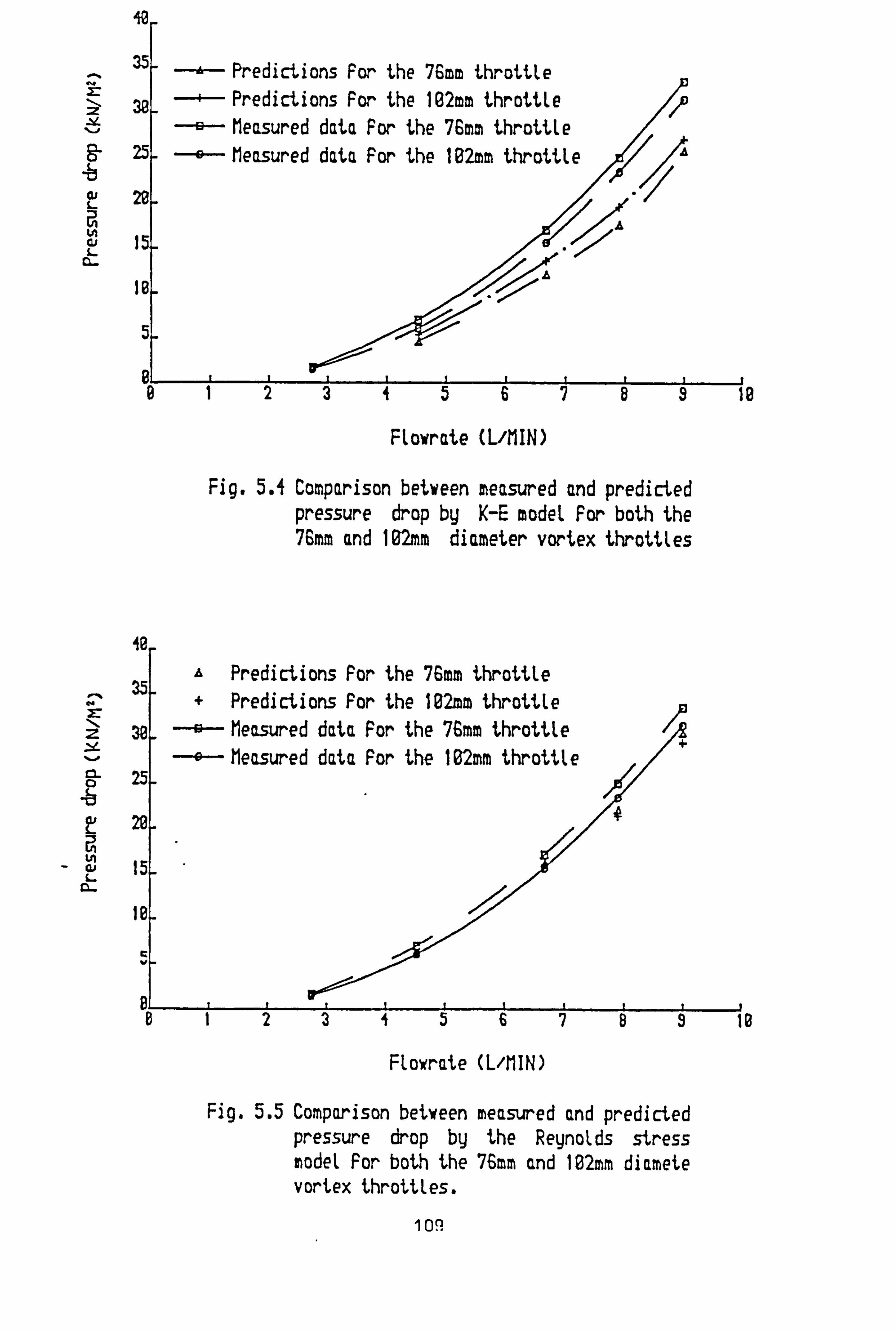
s 3
C,
a L Cl..
40
-a- Predictions For the 76mm throttle --ý- Predictions For the 102mm throttle ' --ý- Measured data For the 76mm throttle --$- Measured data For the 1H2mm throttle
/°
P
78
Flowrate (L'MIN)
Nc
2 V
C. 0
L
Fig. 5.4 Comparison between measured and predicted pressure drop by K-E model for both the 76mm and 102mm diameter vortex throttles
A Predictions For the 76mm throttle + Predictions For the 102mm throttle
--ý- Measured data For the 76mm throttle
-e-- Measured data For the 1E2mm throttle
4567E
Flowrate (L/t1IN)
/, 4
Fig. 5.5 Comparison between measured and predicted pressure drop by the Reynolds stress model For both the 76mm and 102mm diamete vortex throttles.
109
a
9
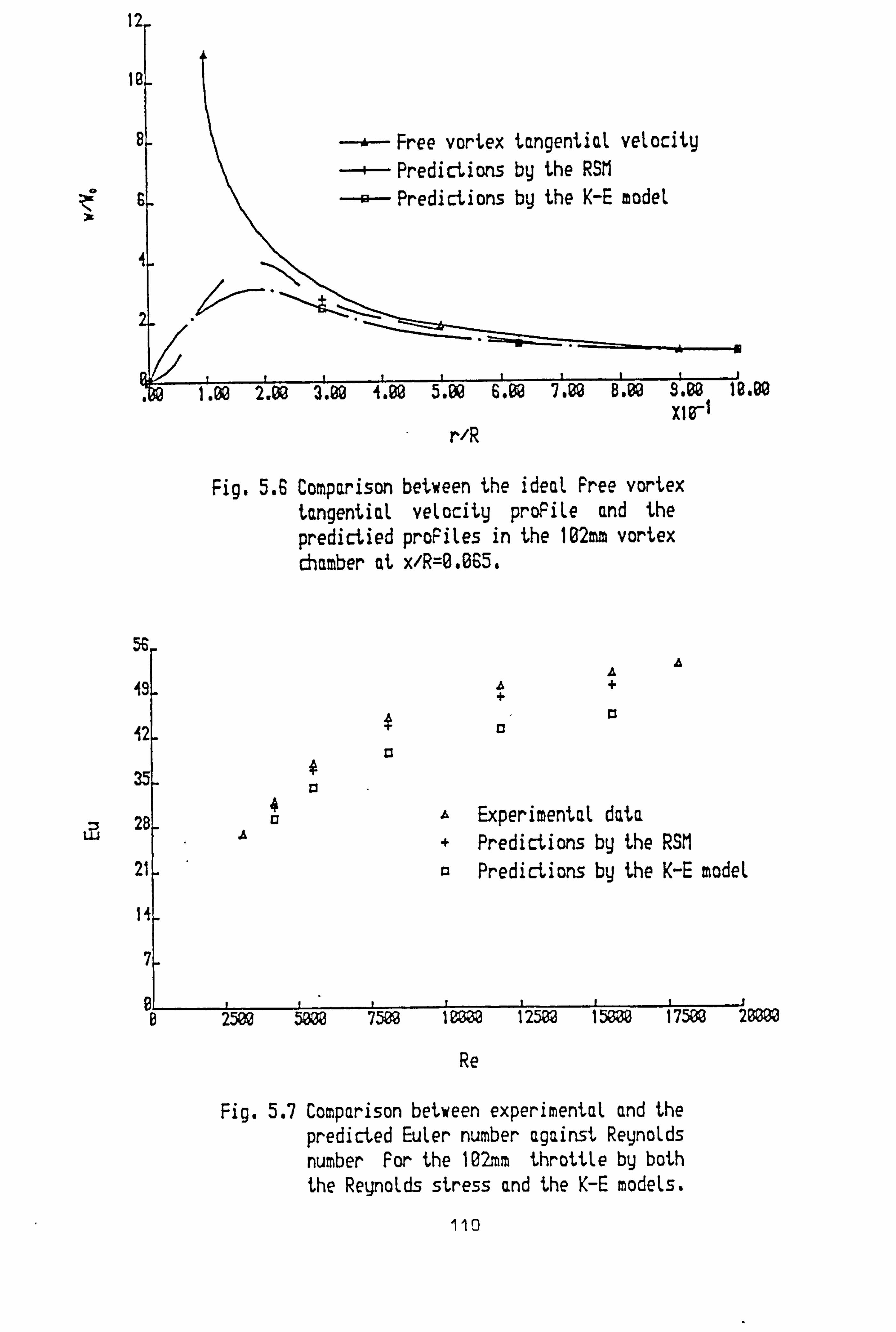
0
i
-+- Free vortex tangential velocity --+- Predictions by the RSM
--ý- Predictions by the K-E model
.. 1.
ýýýý ý.
4.02 5.00 6.02 7.22 8.00 9.68 18.00 X16-,
r/R
w
5ä
Fig. 5.6 Comparison between the ideal Free vortex tangential velocity proPile and the predictied proPiles in the 162mm vortex chamber at x/R=0.065.
a Experimental data + Predictions by the RSM 13 Predictions by the K-E model 21
1'1
1 7500 1 2ßa 12502 15000
Re
e A
A+
n An n
n äA Experimental data
%1 n__J: ýl: __- L.. IL_ ne
Fig. 5.7 Comparison between experimental and the predicted Euler number against Reynolds number For the 102mm throttle by both the Reynolds stress and the K-E models.
110

s
. ýc
3.02 X1r1
r/R
Fig. 5.8 Turbulent kinetic energy proFiles in the 162a, m vortex chamber predicted by the R5M and the K-E model respectively at x/R=0.065.
111

ýý
-ýý
ý(M/S) 4
The RSM predictions The K-E predictions
Fig. 5.9 The tangential velocity proFiles predicted bg both models in the 102mm throttle at Re=11078.
H The RSM predictions The K-E predictions
Fig. 5.10 The axial velocity proPiles predicted by both models in the 102mm throttle at Re=11078.
112
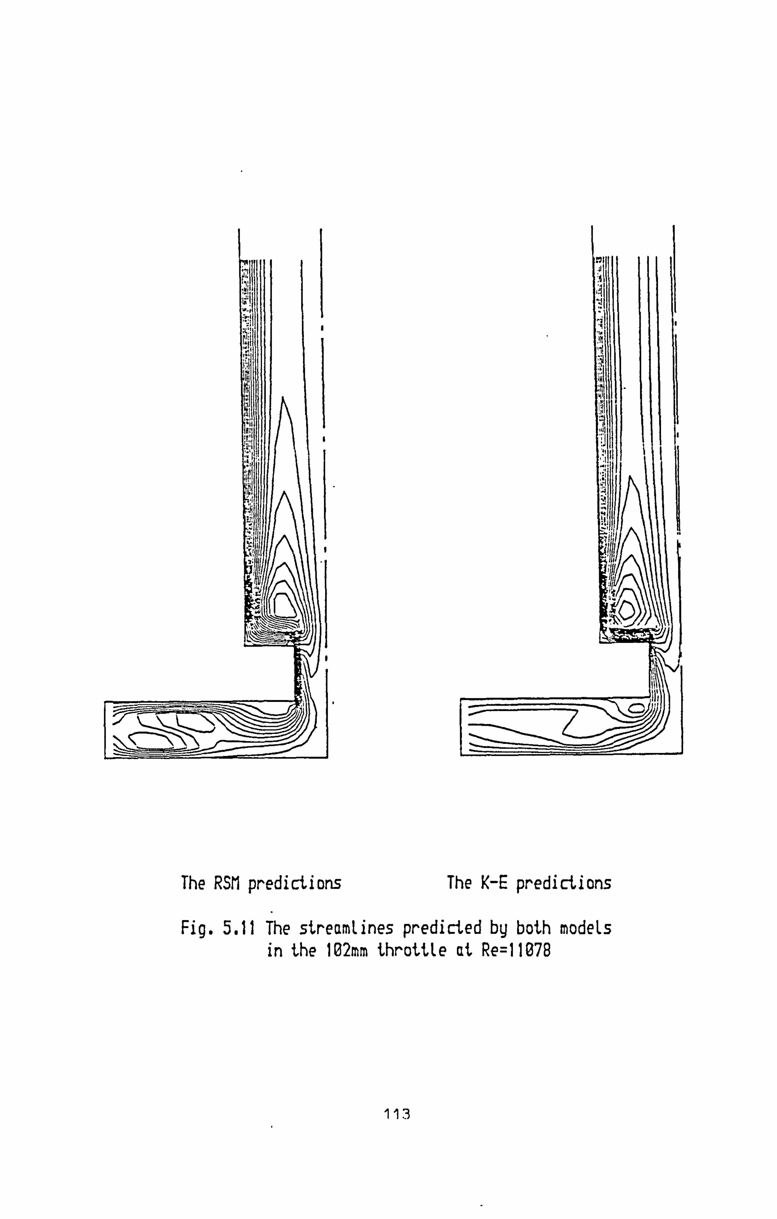
The RSM predictions The K-E predictions
Fig. 5.11 The streamlines predicted by both models in the 102mm throttle at Re=11078
113

i
--------- ii
i --------
f
50 (kM/Mz)
25
Pro=files Contours
Fig. 5.12' The pressure proFiles and contours predicted by the Reunolds stress model in the 102rm throttle at Re=11078
r
Q E
y
i
114

it I. gill 1ý1tý.
. ýrl! It..
. rttlý iitý.
rtltý Itr
rtll lir..,
rtil rir..
"ýlll Iltý.
.. t ;. ; 'ý X11!
rlllý Ilr. ýrll! ilr.,,
tl1lý ilr.., tlýl1
? yyv
...........
. ....
The streamlines The velocity vectors
Fig. 5.13 The streamlines and velocity vectors predicted by the K-E model in the 102mm throttle at Re=5565.
115

R 2385
Re=11376
Fig. 5.14 The stnea. -Aines rodet in the1 Retmo! ds numbers.
R: =55 5
Re=14äe0
predicted by the K-E throttle at ditH erent
116

SI=32
SI=5
SI=15
SI=1
Fig. 5.15 The streamlines predicted by the K-E node. in the 102mm throttle at diFFerent inlet Swirl Intensity (SI)
117

ýf
iý ýý: ý ý
Fig. 5.16 The contours of turbulent kinetic energy dissipation rate predicted by the RSM in the 102mm throttle at Re=11078.
115

Chapter 6
APPLICATIONS TO
COMPRESSIBLE FLOWS
In this chapter, the prediction procedure is applied to steady compressible sub-
sonic, transonic and supersonic flows. The prediction procedure is tested for
accuracy against known analytical solutions for inviscid subsonic, transonic and
supersonic flows in convergent and divergent nozzles. The accuracy of this nu-
merical scheme is further assessed by comparing the results with those obtained
using Godunov first and second-order methods (104) for two dimensional sub-
sonic, transonic and supersonic flows in a channel with a circular arc bump. This
problem was selected as a test case for a workshop (105) and since then has be-
come a standard test problem. The prediction procedure has also been applied
to a more severe case, i. e., supersonic flow behind a rearward-facing step where
a recirculating subsonic flow region is embedded.
The results obtained clearly indicate that the prediction procedure is able to
119

handle laminar subsonic, transonic and supersonic flows. However, when com-
pressible turbulent flows are considered additional problems related to the mod-
elling of turbulence may arise so that turbulent flows are not considered as test
problems in the present study.
6.1 Governing Equations
The governing equations employed are the two dimensional Navier-Stokes equa-
tions which, in the case of inviscid flows, are actually the Euler equations. In
addition, the energy equation and the state equation are also needed. The gov-
erning equations have already been presented in chapter three, and they can be
found in many textbooks and articles (2,25,58,59,60,106).
6.2 Convergent and Divergent Nozzle Flows
The convergent and divergent nozzle flows were selected as the first test problem
mainly because the analytical results are available for comparison with the numer-
ical solutions. Moreover, the flow fields are relatively simple so that the accuracy
of the numerical scheme can be assessed more correctly from the comparison
between the analytical results and the numerical solutions, and confidence can
be gained from this about the capability of the prediction procedure to handle
subsonic, transonic and supersonic flows.
120
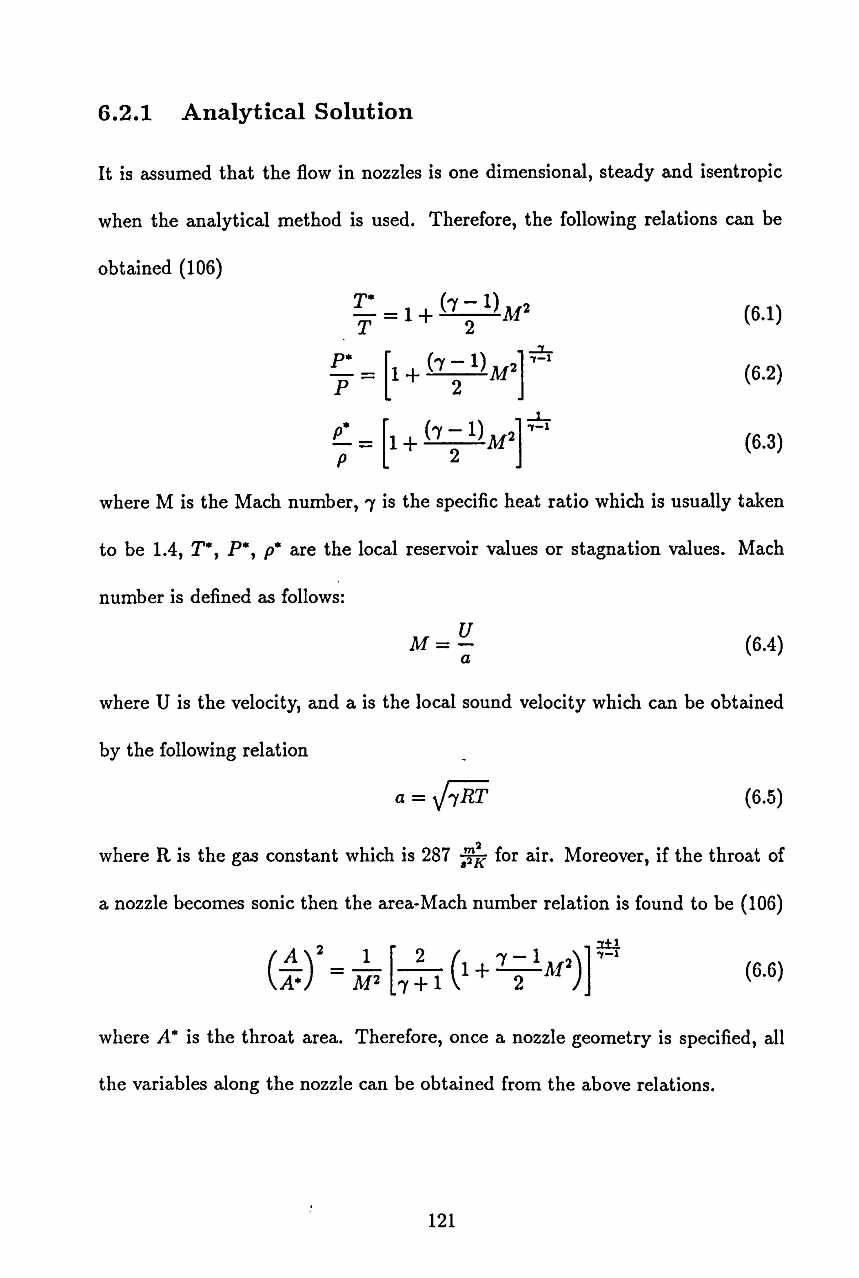
6.2.1 Analytical Solution
It is assumed that the flow in nozzles is one dimensional, steady and isentropic
when the analytical method is used. Therefore, the following relations can be
obtained (106)
T` (ry - 1) Z T, +2M (6.1)
P` =1+
(-1 1)M2 (6.2) PI2
P` =
r1 +
(ry 1) M2
l'_1 (6.3)
P2 lJ where M is the Mach number, y is the specific heat ratio which is usually taken
to be 1.4, T*, P*, p* are the local reservoir values or stagnation values. Mach
number is defined as follows:
M_U a
(6.4)
where U is the velocity, and a is the local sound velocity which can be obtained
by the following relation
a= yRT (6.5)
where R is the gas constant which is 287äK for air. Moreover, if the throat of
a nozzle becomes sonic then the area-Mach number relation is found to be (106)
a_I AJ Mz
[7+i (i+ 721 M2)] 7-1 (6.6) CA*
where A* is the throat area. Therefore, once a nozzle geometry is specified, all
the variables along the nozzle can be obtained from the above relations.
121

6.2.2 Numerical Solution
Calculations of the inviscid subsonic, transonic and supersonic nozzle flows were
performed assuming two dimensional axisymmetrical flows with the tangential
velocity equal to zero. In addition, the stagnation enthalpy was constant as
inviscid and adiabatic flows were assumed so that there was no need to solve the
energy equation.
The stagnation values were taken to be
T* = 303 K (6.7)
P' = 100000 N/n2 (6.8)
The inlet conditions could be worked out by the relations presented in the section
on the analytical solution. They are given as follows:
For the subsonic and transonic flows
M1 = 0.24 (6.9)
Pin = 96070 N/m2 (6.10)
Tin = 300 K (6.11)
Uin = 83.3 m/s (6.12)
For the supersonic flow
Min = 1.17 (6.13)
Pin = 42870 N/rn2 (6.14)
Tin = 238 K (6.15)
U; n = 361.8 m/s (6.16)
122

Geometry of Nozzles
Fig. 6.1 shows the geometry of the nozzles used in this study. The subsonic flow is
obtained in the convergent nozzle, the supersonic flow is produced in the divergent
nozzle and the transonic flow is created in the convergent and divergent nozzle
by specifying appropriate inlet and outlet boundary conditions. The details of
dimensions are given in millmeters as follows:
The convergent nozzle
D1 = 31.6 D2 = 20 L= 35
The convergent-divergent nozzle
D1=31.6 D2=20 L=70
The divergent nozzle
Dl = 20.22 D2 = 31.6 L= 35
Boundary Conditions
Proper specification of the boundary conditions is a crucial aspect in computing
compressible flows. There are, unfortunately, only a few cases where mathemati-
cal theory can tell us what boundary conditions should be imposed so as to ensure
the uniqueness of the solution. Hence, boundary conditions for compressible flows
are usually treated in a heuristic way. Nevertheless, an FDE solution with math-
ematically inconsistent boundary conditions may still give an approximation to
the PDE.
The wall and symmetry boundary conditions for compressible and incom-
pressible flows are more or less the same, and they are fully discussed in reference
123

(2). Therefore, the discussion here will focus on the inlet and outlet boundary
conditions for not only the nozzle flows but also for compressible flows in general.
Inlet Boundary
It is generally accepted that if the inflow is supersonic, all the variables must
be specified at the inlet boundary. However, when the inflow is subsonic, there
are different choices as to which variables are specifi ed. For a two dimensional
subsonic flow, the system of partial differential equations requires three bound-
ary conditions (107). In addition, the numerical methods need a fourth boundary
condition. There are, therefore, basically two ways of specifying the inlet bound-
ary conditions. One is to specify three boundary conditions which are usually
the velocity components along with either density or temperature, and the fourth
boundary condition is extrapolated (107). Another is to specify the inlet bound-
ary conditions completely (2,107). This is a stable boundary condition and
stated as overspecification of the inlet boundary in (107). Nevertheless, most of
the published two dimensional compressible flow computations have adopted this
method. More detailed discussion is given in (107).
In the present study of subsonic nozzle flow, the stagnation pressure, the
stagnation temperature, the inlet Mach number and the inlet flow angle were
given so that the inlet velocity components, inlet density and inlet temperature
could be worked out using the relations presented in the section on the analytical
solution. The inlet boundary conditions were specified completely in the present
calculations.
Outlet Boundary
124

For a two dimensional subsonic outflow boundary, the partial differential equa-
tions require one boundary condition and the numerical solution requires three
additional boundary conditions. Usually, the static pressure is specified and other
variables are extrapolated. However, in some cases, when nothing is available at
the outlet boundary, all variables have to be extrapolated. This is not correct
mathematically and it was pointed out in (107) that the steady-state solution de-
pended strongly on the initial flow field. Detailed discussion about the subsonic
outflow boundary conditions is given in (107).
In the present study of the subsonic nozzle flow, density was specified at the
outlet boundary. The axial velocity was adjusted until the overall mass flowrate
was satisfied. Other variables were extrapolated.
For supersonic flow, there is a general point that outlet boundary conditions
are not important if the outflow is supersonic since supersonic flow limits the
upstream effect. However, this is incorrect as argued by Roache (2), and the
present author, having some experience in supersonic computations, agrees with
Roache's arguments. As stated by Roache (2); if the boundaries had no effect
at all, it would be impossible to "turn off "an indraft supersonic wind tunnel.
It is also stated in (2) that the downstream outflow problem is more important
in supersonic flow than in subsonic flow. The above statements are not diffi-
cult to understand when one considers quasi-one-dimensional inviscid flow in the
convergent-divergent nozzle as shown in Fig. 6.1, where the inlet boundary con-
ditions are fixed. The back pressure can have great influence on the flow pattern
in the nozzle. When the outflow is already supersonic, a reduction in the back
125

pressure will not be felt upstream. However, if the back pressure is raised, a
shock wave will move into the nozzle, its final position depending on the back
pressure. If the back psressure is further raised above a critical value, the flow
will become subsonic through the whole nozzle. Therefore, in Crocco's (108)
calculation of quasi-one-dimensional flow in a duct, two downstream variables,
pressure and temperature, had to be specified to approach a steady solution.
Benison and Rubin (109) also had to fix density at the outflow boundary in their
quasi-one-dimensional calculations. More detailed discussion is given in (2).
In the present study, it has been found that at least one variable, either
static pressure or density, has to be specified at the outlet boundary, and in
the calculation, density was fixed at the supersonic outflow boundary. Other
variables were extrapolated and the axial velocity was adjusted to satisfy overall
mass conservation.
6.2.3 Results and Comparison
When the numerical solutions are compared with the one dimensional analytical
results, the average value of the numerical solutions at each x location is taken.
This is because the numerical solutions are two dimensional.
Subsonic Flow
Fig. 6.2 shows the predicted Mach number profile and the analytical result for
the subsonic flow in the convergent nozzle. Two grid sizes were used to make sure
that the solution is grid independent. It can be seen that very good agreement
126

between the predictions and the analytical solutions has been achieved, and the
results obtained by different grids are almost the same. This means that the
numerical solutions are independent of the grid size and the results are reliable
in this respect.
Fig. 6.3 compares the predicted pressure profile with the pressure profile
obtained by the analytical method for subsonic flow in the convergent nozzle.
It can be seen from the figure that the agreement between the predictions and
the analytical solutions is again very good. This indicates that the prediction
procedure performs quite well for subsonic steady inviscid nozzle flow.
Transonic Flow
For the transonic and supersonic flows, only one grid size was used since the
numerical solutions for the subsonic flow, as shown above, changed very little
when different grid sizes were used.
Fig. 6.4 compares the predicted Mach number profile with the Mach number
profile obtained by the analytical method for transonic flow in the convergent-
divergent nozzle. Good agreement can be seen from this figure, however, near
the throat where a transonic flow region exists, the predicted Mach number is a
little bit lower than the analytical result. This may be partly due to the fact that
the geometry is not simulated exactly since step grids were used instead of using
body fitted coordinates, and partly due to the switch of the different numerical
schemes for density evaluation.
Fig. 6.5 shows the predicted pressure profile and the pressure profile obtained
127
by the analytical method along the convergent-divergent nozzle. The agreement
is, as can be seen from the figure, quite good overall apart from the near throat
region where the predicted pressure is higher than that obtained by the analytical
method. This corresponds to the prediction of the Mach number in this region
discussed above.
Supersonic Flow
Fig. 6.6 compares the predicted Mach number profile with the analytical Mach
number profile for supersonic flow in the divergent nozzle. As can be seen from
the figure, generally good agreement has been reached but not as good as that
for the subsonic flow. This may be attributed partly to the use of the step grids
and partly to the reason that the prediction procedure cannot fully simulate the
nature of supersonic flow as stated before.
Fig. 6.7 shows the predicted pressure profile together with the pressure profile
obtained using the analytical method. Once again only a general good agreement
has been achieved, which corresponds to the prediction of the Mach number as
shown in Fig. 6.6.
Fig. 6.8 and Fig. 6.9 show the predicted velocity vectors in the convergent
and the divergent nozzles respectively. It can be seen from the figures that the
flows are almost one dimensional in both cases since the radial velocity is quite
small compared with the axial velocity. This indicates that the assumption of
one dimensional flow in the nozzles is very close to reality.
From the above results it can be said that the prediction procedure performs
128
quite well for the subsonic, transonic and supersonic steady inviscid nozzle flows.
However, further tests in different flow situations should be made to assess the
general validity of the prediction procedure.
6.3 Channel Flow
The second test problem chosen in this study is the two dimensional subsonic,
transonic and supersonic flow in a channel with a circular arc bump on the lower
wall. This problem was selected to assess the accuracy of the prediction procedure
since it is a standard test problem as stated before, and it is well suited for
computer code development and testing. In addition, there are results obtained
by Godunov first- and second-order methods available for comparison with the
present numerical solution.
6.3.1 Geometry of the Channel
Fig. 6.10 shows the channel used in the present study. It has a circular arc bump
on the lower wall. The distance between the upper and the lower walls is equal to
the chord length. The total length of the channel is three times the chord length.
Two circular arc bump thickness-to-chord ratios were used in the study: 10% for
the subsonic and transonic flow modelling, 4% for the supersonic flow modelling.
Step grids were used to simulate the geometry of the circular arc bump.
129
6.3.2 Boundary Conditions
A detailed discussion on the boundary conditions for compressible flow has been
presented in the previous section. It is argued that one variable should be specified
at the outlet boundary for not only subsonic flow but also for supersonic flow if
possible. For the flow considered here in the channel, at the inlet, the total
temperature, the total pressure and the Mach number were specified. Density
was specified at the outlet boundary. The axial velocity was adjusted until the
overall mass flowrate was satisfied.
6.3.3 Results and Comparison
Fig. 6.11 compares the predicted Mach number profile with the results obtained
by the first- and second-order Godunov methods (104) at the lower wall of the
channel for subsonic flow. It can be seen from the figure that good overall agree-
ment has been achieved. However, at around the mid-chord the prediction pro-
cedure overpredicted the Mach number by about 3%. This may be attributed
to the use of the step grid to simulate the circular arc bump. Near the outlet,
the present prediction is much closer to the results obtained by the second-order
Godunov method compared with the first-order Godunov method.
The comparison between the present prediction and the results given by the
first- and second-order Godunov methods at the upper wall of the channel is
shown in Fig. 6.12. Very good agreement has been achieved as can be seen from
the figure.
From Fig. 6.11, it could be said that the prediction procedure performed
130
better than the first-order Godunov method as the overall prediction is closer to
the results by the second-order Godunov method. Nevertheless, at around the
mid-chord the result given by the first-order Godunov method is closer to the
result obtained from the second-order Godunov method. In addition, one can
hardly distinguish the difference between the present prediction and the result of
the first-order Godunov method from Fig. 6.12. Therefore, it is fair to say that
the prediction procedure is onl? first-order accuracy in the case of subsonic flow.
For transonic flow, the comparison between the present prediction and the
results obtained by the first- and second-order Godunov methods at the lower
wall and the upper wall of the channel are presented respectively in Fig. 6.13
and Fig. 6.14.
Fig. 6.13 shows the results at the lower wall of the channel. In this case, a
supersonic flow region appears around mid-chord and is terminated by a shock
at about two-thirds length of the chord. It is seen that the prediction procedure
underpredicted the shock strength by about 8% compared with the second-order
Godunov method. However, the results obtained by the first-order method agree
very well with the present prediction. This indicates that in the case of transonic
o flow the prediction procedure is also-'first-order accuracy.
Fig. 6.14 compares the present prediction with the results by the Godunov
methods at the upper wall. As can be seen from the figure, the overall agree-
ment between the prediction and the results obtained by the first-order Godunov
ce method is better which confirms that the prediction procedure is first-order ac-
curacy.
131

Fig. 6.15 compares the prediction of Mach number with the results by the
first- and second-order Godunov methods at the lower wall for the case of su-
personic flow. In this case, there is an oblique shock wave at the leading edge
of the circular are bump. It can be seen from Fig. 6.15 that Mach number
dropped suddenly at the leading edge which indicates that the oblique shock
wave is predicted. However, the present prediction is rather poor compared with
the results obtained by the second-order Godunov method but comparable with
the results by the first-order Godunov method. At the end of the circular arc
bump, i. e., at the trailing edge, a shock wave also exists. This can be also seen
from the figure since there is another sudden drop of Mach number. The present
prediction is again rather poor compared with the results by the second-order Go-
dunov method and can only be comparable with those by the first-order Godunov
method.
Fig. 6.16 presents the comparison at the upper wall of the channel for the same
case. The results by the second-order Godunov method show a very sharp drop
of Mach number at about two-thirds of the channel length where the oblique
shock wave formed at the leading edge intersects the top wall. However, the
present prediction is rather poor even compared with the results by the first-order
Godunov method. The shock wave is too oversmeared by the present prediction
procedure as can be seen from Fig. 6.16. This indicates that in order to get good
resolution of shock waves alternative numerical techniques have to be employed.
It can be seen from the above comparative study that the present prediction
procedure is only comparable with the first-order method. The overall predictions
132

are, generally speaking, quite good but some other special numerical technique
has to be employed in order to get a better prediction of supersonic flow with
strong shock waves.
6.4 Flow Behind a Rearward-Facing Step
The previous test cases have clearly demonstrated that the prediction procedure
can handle the quasi-one dimensional subsonic, transonic and supersonic nozzle
flows. For two dimensional subsonic, transonic and supersonic flows in the channel
with a circular arc bump, overall good agreement has been achieved between
the present predictions and the results obtained by the Godunov methods. In
this section, in order to check the general validity of the prediction procedure
a more complicated flow case is chosen as a more severe test for the prediction
procedure. This is supersonic laminar flow behind a rearward-facing step with a
subsonic recirculating flow region. This kind of flow can be found in important
engineering applications such as the flow in a supersonic combustor.
6.4.1 Flow Geometry
Fig. 6.17 shows the flow geometry under investigation. The Reynolds number of
the laminar approach flow at the step is 1.2 x 10⁶ which corresponds to a static
pressure of 2900 Pa and a static temperature of 80 K (32). The air inflow Mach
number is 3.5 which corresponds to a inlet velocity of 627.5 m/s at the step.
133

6.4.2 Boundary Conditions
The specification of computational boundary conditions for compressible flow has
been fully discussed above. For this particular case, the velocity, static pressure
and temperature were specified at the inlet boundary and density was specified at
the outlet boundary. The no-slip boundary condition was applied at the wall and
reflection boundary conditions as presented before were employed for the upper
boundary.
6.4.3 Results and Comparison
Fig. 6.18 presents the comparison between the predicted wall pressure distribu-
tion and the experimental data (32) behind the step. The pressure was normal-
ized by the inflow static pressure. It can be seen from the figure that quite good
agreement has been achieved.
Fig. 6.19 compares the predicted static pressure profile with the experimental
data at a location downstream of a step at x/h = 0.0537. The pressure was
normalized by the inflow static pressure. An overall good agreement has been
obtained as shown in the figure.
Fig. 6.20 and Fig. 6.21 presents the comparisons between the predicted
normalized static pressure profiles and the experimental data at locations down-
stream of steps at x/h = 2.137,4.279. It can be seen again that general overall
good agreement has been achieved. However, there are some discrepances be-
tween the predictions and the experimental data near the wall. This may be at-
tributed to the fact that the flow attaches to the lower wall between two locations
134
and hence more complicated phenomena such as a shock wave, flow separation
and transition may occur which the prediction procedure cannot simulate exactly.
Fig. 6.22 presents the predicted velocity vectors. It can be seen that the
flow field near the upper boundary does not change much. This verifies that it is
appropriate to employ the reflection boundary conditions for the upper boundary.
6.5 Closure
The prediction procedure has been applied to several compressible flow cases
which include subsonic, transonic and supersonic flows. The one crucial issue in
computing compressible flow is the specification of the computational boundary
conditions. These are, in particular, of great importance for supersonic flow as
the established principle is misleading. The results shown above confirm that the
prediction procedure can not only handle simple quasi-one dimensional subsonic,
transonic and supersonic flows but also can predict quite well two-dimensional
subsonic, transonic and supersonic channel flows and the even more complicated
supersonic flow behind a rearward-facing step with a subsonic recirculating flow
region. However, the present prediction procedure cannot give good resolution of
shock waves. This indicates that other numerical techniques have to be employed
in order to get a better prediction of supersonic flow with shock waves.
135
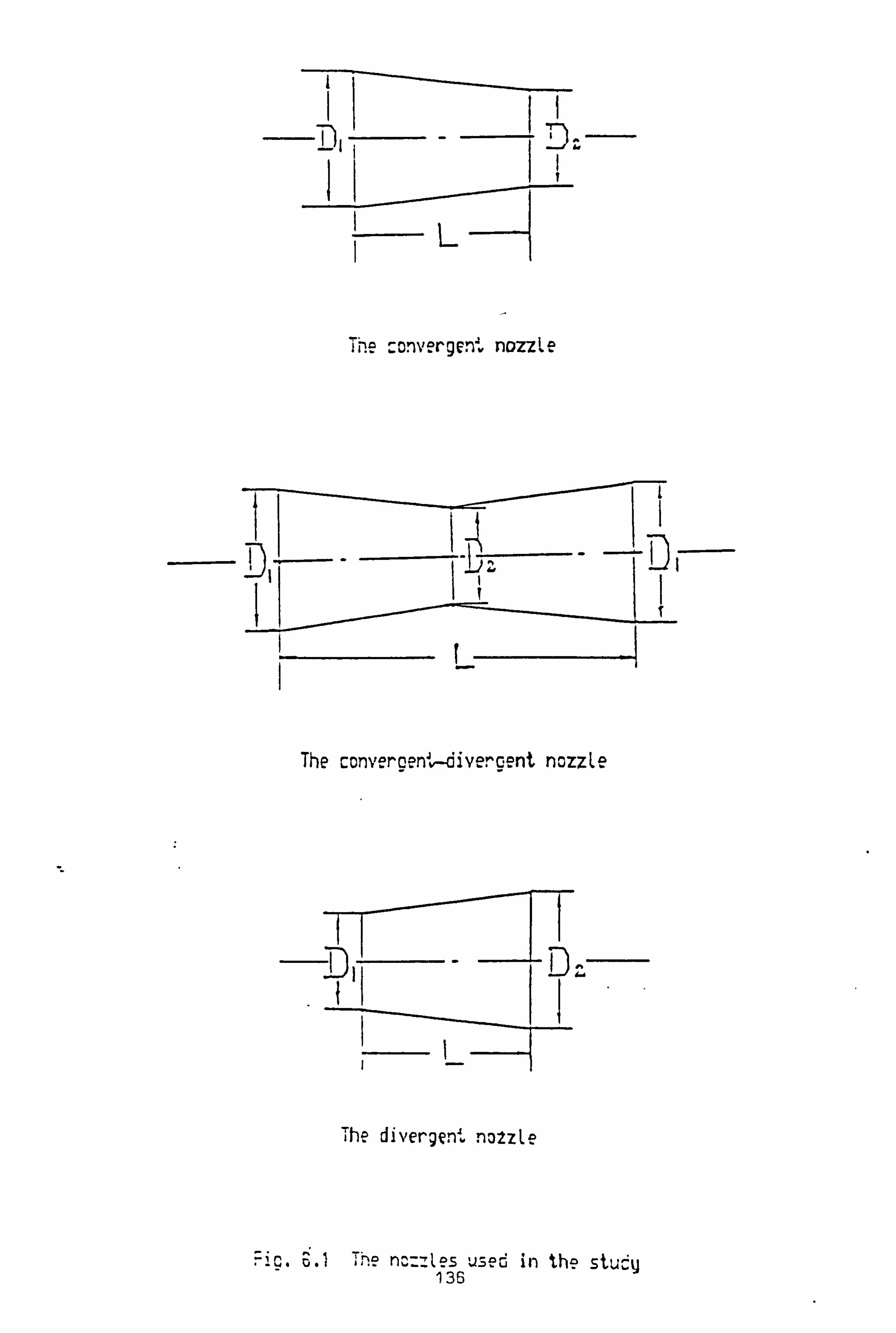
t
i1 Dz 1
! he convergence nozzle
t
ý IJ
r
The convereen'�-divercent nozzle
TT The divergent no2zle
Fiy, ö. i he ncý=las used in the study 136

e. ez!
ß. e21 ö. eu=
5. eel
I . ee_
1
The cnc; u: iCal. resL: t The precis ion by the 27'43 cris the predi- ion by the 1BY43 grid
0
. VV
. ea 1. e2 2. ee 3. e0 4. ee :..
1/L
.c7.2 8. C3 5.02 IC. B2 x12-1
=iS2 r Mnnrý Dei: e nr
. G. ý ýo ýý, son between ýý ?rýc Mach, nunoer pro=i1e cnd the cnclyticcl result in the converoent nozzle.
X1e-1 10.02-
S .'
-The onciu icat result 7.00 The prediction by the 27}43 grid
s ; a The prediction by the 18M grid
M - ý
5.00
S. eOý
3.62
ýz t. & 2. eß 3.02 4. B? 5.22 E. 02 ;. ea E. e7 °. 03 tc. ce X10-1
I/L
Fig. 6.3 Comparison between the predicted pressure pro=ile and the cn¢tutical result in the converoent nozzle.
137
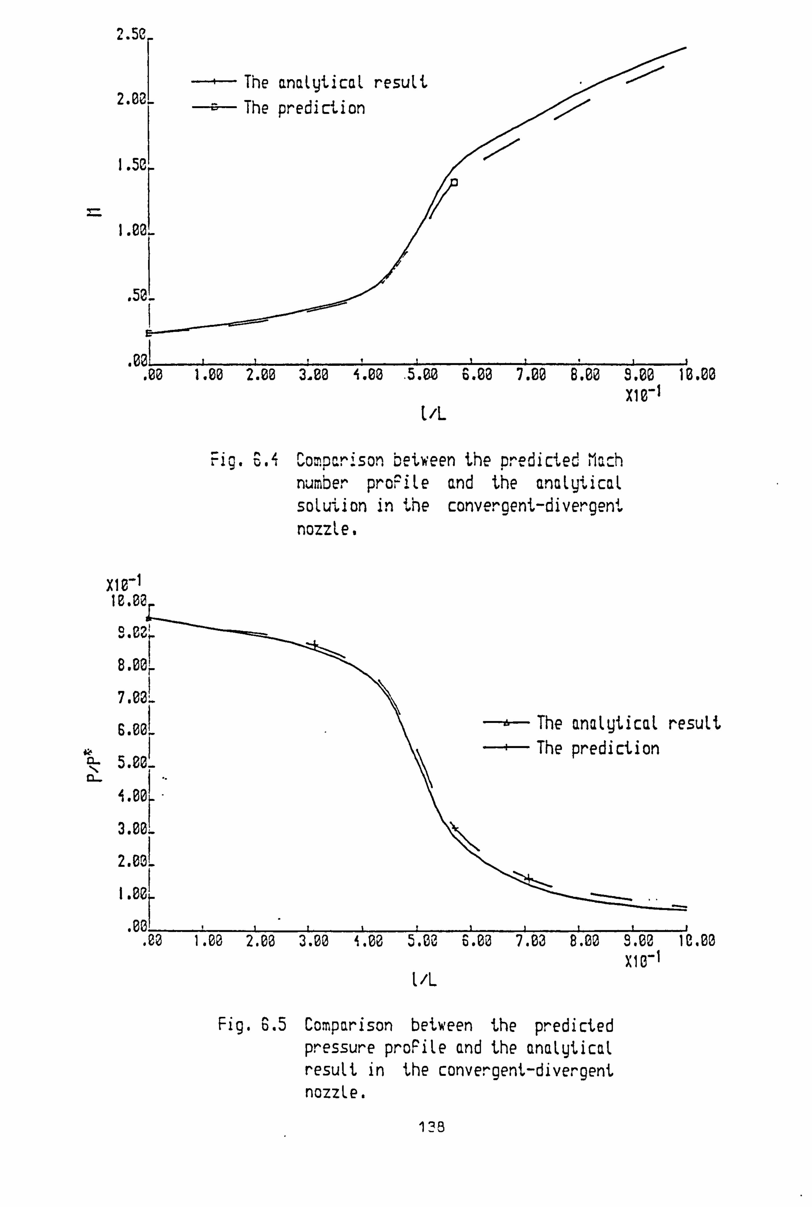
2.50
2.00_
1.50
1.00
. 52_
. vv
. 00 1.00 2.00 3.00 4.00 . 5.00 6.02 7.00 8.06 5.00 16.06 X10⁻¹
IIL
Fig. E. 4 Comparison between the predicted Mach number prorile and the analytical solution in the convergent-divergent nozzle.
z1e-1 10.00
s. e2ý 8.00r
7.001 6.001 -ý- The analytical result
k -ý- The prediction 5.00- rL- I 4.00
3..
2.001
1.001
. 00 1.00 2.00 3.00 5.00 5.00 6.00 7.03 8.00 3.00 10.00 X10⁻¹
t/L
Fig. G. 5 Comparison between the predicted pressure proFile and the analytical result in the convergent-divergent nozzle.
1? B

2.50
2.20,.
1.92
1. ö0_
i
The analytical result The prediction
1.30
. 00 1.00 2.80 3.00 4.00 5.00 6.00 7.00 8.00 8.00 10.00 X10⁻¹
l/L
Fig. 0.6 Comparison between the predicted Mach number proFile and the analytical result in the diveroent nozzle.
xi -1 5.00
4.
3.80E N
12-
nom. \ 2.00L
The analytical result -{ý- The pediction
---- 12 1.00
. 00 1.00 2.03 3.03 1.03 5.00 6.00 7.00 8.00 9.03 10.03 X10⁻¹
l/L
Fig. 6.7 Comparison between the predicted pressure proFile and the analytical result in the divergent nozzle.
139
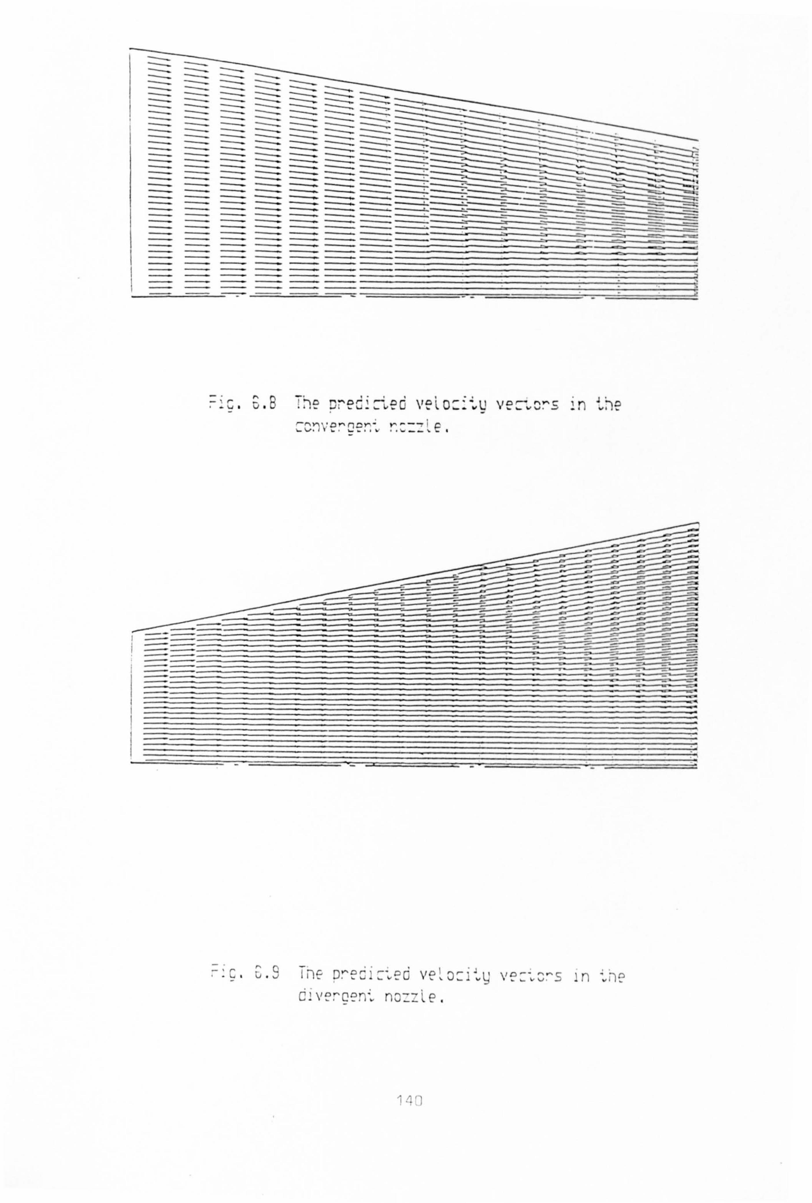
1 !1 ß`1e
IlE D"°G1G °_G V°: OG: h \'e: . ̂5 In ne cive^epn. nc_; e.
111

L
13.10 The channel with a circular arc bump used in the study.
141

X1e-1 10.00 s. eer 6.001
2. ear 6.00_
= 5. eß. 9.02E
3.20!
2.001
ý . eý:.
--- The predicted proFile o Results by the second-order method + Results by the First-order method
0 1
++
. 00 1.00 2.00 3.00 4.00 5.00 6.00 7.00 8.00 9.00 X10⁻¹
, /L
Fig. 6.11 Comparison 5eiween the predicted Mach number pro=ile a-;, the Lower waU. and the results obtained by the First and second-order Godunoýý Methods for the subsonic Fiow.
X10-1 10.00
s. oo! The predicted pro^ile
a Results by the second-order method LOA Results by the =ir5t-order method 6.00'
r 5.0
4.001
3.00
2.00 . 00 1.00 2.03 3.00 4.00 5.00 6.02 7.03 B. 00 5.03
X10-1 l/L
Fig. 6.12 Comparison between the predicted Mach number proFile at the upper wall and the results obtained by the First and second-order Godunov methods For the subsonic Flow.
. 00
. 02
142

ý"Býý- -- 1 The predicted proFile + Results bg the second-order method a Results by the first-order method 1.40E
+ . 26ý
1.001
+
/o
. 86i p
. 00 1.00 2.80 3.00 4.00 5.03 6.80 7.20 8.03 5.00 10.00 X10'1
. IL
Fig. C. 13 Comparison between the predicted Mach number proFile at thºe tower wall and the results obtained bg the First and second-order Godunov methods For the transonic Flow.
xla_, f2.33i
n. n --ý-- The predicted proFile + Results by the second-order method
10.221. Resui is by the first -order method 9.33-
8.44! yn
7.56;
0.6 '
5.78!
4.89_
A 1. N 2.03 3.33 4.03 5.03 6.03 7.03 8.00 5.03 10.03 X10⁻¹
ý/L
Fig. 6.14 Comparison between the predicted reach number pro°ile at the upper wall and the results obtained by the First and second-order Godunov methods For the transonic Flow.
143

2"1er -+- The predicted proFile a Results by the first-order method
ý, 9eý o Results by the second-order method
1.76 /° 000
n ° 1.5ýý
0
I. 101 1 "J- t --' 1 1- . 03 1.03 2.00 3.00 '.. 20 5.00 6.00 7.00 8.00 S. 03 10.00
X10', l/L
Fig. £. 15 Comparison between the predicted Mach number pro=ile and the results obtained by the First and second-order Gudonov methods at the lower wall in the case of supersonic Flow.
2.10
I. 90;
1.70
1. Sß1
0 00
ß. 3aß o
. e0 1. e0 2.00 3.02 1.00 5.03 6.00 7.03 8.00 3.00 x10-I
L I/
Fig. 6.16 Comparison between the predicted flach number proFile and the results obtained by the First and second-order Gudonov methods at the upper wall in the case of supersonic Flow.
144
The predicted profile n Results by the First-order method
Resulis by the second-order method 0
. ea

Fcs=2.900 KPc
S=sDK Re=1.2>aCý(! oMlnor)
Yi JhLScm
I---- X
Bio. 6.17 glow oeomeira.
_LL
^Z
0 X/il
Fig. 6.18 Comparison between the predicted wall pressure distribution and experimental dc a For the supersonic Laminar Flow over a rearw"arc-=ccin; step.
145

, 80I r
the predicted pressure proFile 02,1 a Experimental data
, 4D!
1y i
. ea" , ai 2 3 4
g/h
F i;. 6,19 Comparison between the predicted pressure pro=i; e and experimental data For the supersonic Laminar Flow behind a rearward-"acing step at xJh=0.0537.
1.00-
N
CL! LL
Cl-
yih
Fig. 6.20 Comparison between the predicted pressure proFile and experimental data For the supersonic laminar Flow behind a rearward-Facing step at x/h=2.137.
146

62ý i
Exae"'_Ten-c: aZ
. OIL 223
y/h
: "OC~50`^ 7ý.. Woan ýiý rýnoý" Apr
data '0! " the SUDeer50n. C : aTina ELOh'
rearn'C^C-=CC: n; 5 eD at
X%.. =/ . _? S.
Fig. G . 22 ß; ie prediciec veloc., ý veEtors For, `; ° suoerSOnlC G""nomr "loh' ben'_nd
I:; '

Chapter 7
CLOSURE
In this chapter, the concluding remarks are presented. The discussion will be
divided into two parts. In the first part, a brief review of the whole thesis will
be presented. This is followed by suggestions for further work in regard to the
present study.
7.1 A Review of The Thesis
The main objectives of the present work are stated in chapter one.
1). The first objective is to develop a general elliptical prediction procedure
which is valid for both incompressible flow and compressible flow at any Mach
number. The prediction procedure is based on the SIMPLE algorithm and solves
the steady-state form of the Navier-Stokes equations. In order to make the predic-
tion procedure valid for both incompressible and compressible flows, pressure has
to be chosen as a main dependent variable instead of density. This is in contrast
148

with the time-dependent (unsteady) methods which usually employ density as a
main dependent variable and integrate the unsteady form of the Navier-Stokes
equations to reach a steady state.
2). The second objective is to undertake a comparative study of the two-
equation k-e turbulence model and a Reynolds stress model in the case of strongly
swirling flows in vortex throttles. It was anticipated that Reynolds stress models
would give better performance than the two equation k-E model in such a case.
The work reported in this thesis is summarized as follows to the extent to
which these objectives have been attained.
7.1.1 Turbulence Models
In order to solve the time averaged Navier-Stokes equations, it is necessary to
approximate the correlation terms representing the turbulent shear stresses by
modelling assumptions. Several approaches have been discussed in the previous
chapters. Among these the one-point closure approach has been widely used,
and hence almost all the one-point closure turbulence models have been reviewed
with particular emphases on the two-equation k-e model and the Reynolds stress
model.
The two-equation k-c model, using the Boussinesq assumption, relates the
turbulent shear stresses or the Reynolds stresses to the mean strain through the
turbulent viscosity or eddy viscosity. This turbulence model has been widely used
in engineering calculations. However, the two-equation k-e model (and other two-
equation turbulence models) have several limitations as pointed out in chapter
149

three. One of the practical limitations is the assumption of isotropic eddy vis-
cosity. This affects its performance in the case of strongly swirling flows under
consideration as anistropy then becomes important. In addition, some physi-
cal processes such as those due to streamline curvature, rotation, and buoyancy
forces have to be modelled separately.
Reynolds stress models, however, do not have these limitations as the Boussi-
nesq assumption is not employed and a transport equation is developed for each
Reynolds stress. Moreover, the effects of streamline curvature, rotation, and
buoyancy forces are believed to be accounted for automatically in Reynolds stress
models. They are, therefore, in principle superior to the two-equation k-e model.
However, they have not been thoroughly tested for some complicated flows such
as the very strongly swirling flows under study. In addition, they are more com-
plicated and need enormous computer power.
Both the k-c model and a Reynolds stress model have been applied to the
strongly swirling flows in vortex throttles. The results obtained have confirmed
that the Reynolds stress model gives overall better performance compared with
the two-equation k-E model. The k-c model overpredicted the turbulent kinetic
energy greatly compared with the Reynolds stress model. This could be the
major reason (although there are some other reasons) why the k-e model gives
poor performance in such a case.
150

7.1.2 Numerical Aspects
The control volume method was used to discretize the governing non-linear partial
differential equations. In order to avoid an unrealistic solution the staggered grid
system was employed. The resultant finite difference equations were solved by
a line-by-line iteration method and the variables along each line were obtained
using the TDMA (Tri-Diagonal Matrix Algorithm). The pressure-velocity link
was handled by employing the SIMPLE algorithm.
For compressible subsonic flow, some modifications have been made to the
SIMPLE algorithm to calculate density. It has been found that one variable
(usually static pressure or density) should be specified at the outlet boundary to
ensure a realistic accurate solution.
When supersonic flow is of concern more modifications must be made to ac-
count for the hyperbolic nature of such flow. It has been stated that the eval-
uation of density at the control volume boundaries and the differencing of the
pressure gradient are two important issues. It seems contradictory on one hand
that downstream influences should be eliminated in the case of supersonic flow
and on the other hand a central differencing scheme was still used for the pres-
sure gradient. However, it should be pointed out that the so called downstream
influences refer to some `small disturbances', and it has been stated clearly that
eliminating the downstream pressure influence is misleading, since it would result
in some unrealistic conclusions. As a result of this, it may be fair to say that
the prediction procedure simulates the hyperbolic nature of supersonic flow only
partially as the downstream small disturbances cannot be eliminated completely.
151
Moreover, shocks were oversmeared by the prediction procedure as no special
technique has been employed to handle them.
It has been argued that the pressure-correction equation should be modified
for compressible flow as density changes in such a case. Nevertheless, the ex-
periences gained by the present author has indicated that this is not necessary
provided the density calculation is switched on after a reasonable pressure field
has been established and proper under-relaxation factors are given. In fact, this
means that density change lags one iteration behind which is equivalent to the
treatment of the non-linearities of the momentum equations in the prediction
procedure.
The established principle that no boundary conditions should be specified at
the supersonic flow outlet is questionable. The treatment that all variables at the
outlet boundary are interpolated may be valid in some cases. However, in some
other cases such as the convergent and divergent nozzle flow under study at least
one variable should be specified at the outlet boundary.
7.1.3 Validation of the Prediction Procedure
The prediction procedure was validiated by comparing the predictions with the
known analytical and numerical results in two cases. The first study is the
quasi-one dimensional inviscid subsonic, transonic and supersonic flows in the
convergent, convergent and divergent, and divergent nozzles respectively. The
comparison has been made between the known analytical results and the pre-
dictions. Good agreement has been achieved, especially for subsonic flow in the
152
convergent nozzle where the agreement is very good. The second validation test
is the two dimensional subsonic, transonic and supersonic flow in a channel with a
circular arc bump. This is a standard test problem. On the whole, the prediction
procedure performed well but the shock was oversmeared as pointed out before.
In addition, one factor that would affect the accuracy of the prediction procedure
is that step grids were used to simulate different geometries, and it is believed
that the use of body-fitted coordinates would improve the accuracy.
7.1.4 Applications to Other Cases
The prediction procedure has been also applied to other flow cases; the more
severe and complicated supersonic laminar flow behind a backward-facing step
which has embedded subsonic flow regions was calculated. The predicted pressure
profiles were compared with the experimental data and good overall agreement
was achieved. However, it is difficult to assess the performance of the prediction
procedure in the turbulent case as additional problems related to the turbulence
modelling may arise.
On the basis of the results reported in this thesis, the prediction procedure
is, generally speaking, able to handle subsonic, transonic and supersonic flows.
However, when flow with shocks is of concern the shock resolution is very poor
as no special technique has been employed to handle shocks. Moreover, the
hyperbolic nature of supersonic flow cannot be simulated exactly.
153
7.2 Suggestions for Future Work
The present study has not covered some areas both in depth and breadth. Further
research could be usefully performed to improve the effectiveness of the prediction
procedure and to deepen our understanding of some physical phenomena. Some
examples are as follows:
The present numerical scheme simulates the hyperbolic nature of supersonic
flow only partially. The linkage between each node and the neighboring nodes in
the lateral direction have not been modified. In reality the variables at a certain
location should be affected by the small disturbances only within certain `influ-
ence zones' bounded by the characteristic curves. However, the characteristic
angles vary throughout the flow field and are not known in advance. It is, there-
fore, very difficult but not impossible to construct the required grid to simulate
this feature exactly.
The prediction procedure has not employed any special techniques to handle
shocks, and hence shocks are oversmeared and the shock resolution is very poor.
In order to solve supersonic shock flow successfully it is necessary to employ
a more accurate shock-capturing numerical scheme to evaluate the steady-state
Navier-Stokes equations.
Turbulence modelling is still a great challenge for incompressible flow, let
alone compressible flow. Most turbulence models developed so far are only for
incompressible flow and the literature on turbulence modell ing for the compress-
ible case is much more scarce. There is considerable scope since a great deal of
154
research work in this area needs to be done so as to improve our understanding
of the physical phenomena.
Systematic study should be undertaken to investigate the effects of computa-
tional boundary conditions on the whole solution procedure for compressible flow,
in particular for supersonic flow. It has been stated that the established princi-
ple on the supersonic flow outlet boundary treatment is, in some cases, rather
misleading. However, when there are no variables given at the outlet then what
kind of boundary treatment should be used. The interpolation method may be
valid in some cases but not always. Further study should be done on this aspect.
The flow field in scramjet combustor is very complicated due to highly turbu-
lent reacting mixed supersonic/subsonic flow. It is of great value both for better
understanding of mixed supersonic/subsonic reactive flow and engineering appli-
cations to be able to predict such complicated flow accurately. Further research
work on reacting mixed supersonic/subsonic flow is of great importance to future
long-range commerical aviation and outer-space exploration.
The vortex throttles used in the present study are very effective in producing
a high pressure drop as a result of dissipating the high tangential velocity. How-
ever, in some applications it would be useful to exploit the centrifugal force and
tangential velocity created within a vortex, without the penalty of the high over-
all pressure loss. This would require recovery of the vortex energy, as opposed
to its dissipation as in the throttle. Turbulence usually extracts energy from the
mean flow and dissipates it by viscous action, which is contrary to this objective.
Nevertheless, turbulent kinetic energy is, in most cases, much less than the total
155

kinetic energy. For example, in our case, the turbulent kinetic energy predicted
by the Reynolds stress model in the chamber is only about 3% of the total kinetic
energy. Therefore, Significant energy recovery would be possible if losses due to
the axial recirculation, the sudden expansion at the axial port , and friction losses
within the port, could be minimised.
156

References
[1] Ballhaus, W. F., Jr., Computational Aerodynamics and Design. Eight Inter-
national Conference on Numerical Methods in Fluid Dynamics Proceedings,
Aachen, pp. 1-20,1982.
[2] Roache, P. J., "Computational Fluid Dynamics". Hermosa, Albuquerque,
1972.
[3] Kutler, P., A Perspective of Theoretical and Applied Computational Fluid
Dynamics. AIAA J., Vol. 23, No. 3, pp. 328-341,1985.
[4] Nallasamy, M., Turbulence Models and Their Applications to the Prediction
of Internal Flows: A Review. Computers & Fluids, Vol. 15, No. 2, pp. 151-
194,1987.
[5] Oran, E. S. and Boris, J. P., Detailed Modelling of Combustion System.
Prog. Energy Combust. Sci., Vol. 7, pp. 1-72,1981.
[6] Patankar, S. V. and Spalding, D. B., A Calculation Procedure for Heat,
Mass and Momentum Transfer in Three-Dimensional Parabolic Flows. In-
ternational J. of Heat and Mass Transfer, Vol. 15, pp. 1787-1805,1972.
[7] Patankar, S. V., "Numerical Heat Transfer and Fluid Flow". Hemisphere,
1980.
157
[8] Launder, B. E. and Spalding, D. B., The Numerical Computation of Tur-
bulent Flows. Comput. Meth. Appl. Mech. Engng., Vol. 3, pp. 269-289,
1974.
[9] Chorin, A. J., A Numerical Method for Solving Incompressible Viscous
Flow Problems. J. Comp. Phys., Vol. 2, pp. 12-26,1967.
[10] Harlow, F. H. and Welch, J. E., Numerical Calculation of Time-Dependent
Viscous Incompressible Flow of Fluid with Free Surface. Phys. of Fluids,
Vol. 8, No. 3, pp. 2182-2189,1965.
[11] Donavan, L. F., A Numerical Solution of Unsteady Flow in Two-
Dimensional Square Cavity. AIAA J., Vol. 8, No. 3, pp. 524-529,1970.
[12] Lawal, A. and Mujumdar, A. S., Laminar Flow and Heat Transfer in
Power-Law Fluids Flowing in Arbitrary Cross-Section Ducts. Numerical
Heat Transfer, Vol. 8, pp. 217-244,1985.
[13] Connell, S. D., Numerical Solution of the Equations of Viscous Flow. Ph. D
Thesis, Nottingham University, 1983.
[14] Connell, S. D. and Stow, P., The Pressure Correction Method. Computer
& Fluids, Vol. 14, No. 1, pp. 1-10,1986.
[15] Patankar, S. V., Numerical Prediction of Three Dimensional Flows, in B.
E. Launder (ed. ), Studies in Convection: Theory, Measurment and Appli-
cations, Vol. 1, pp. 1-78, Academic, New York, 1975.
158
[16] Rubini, P. A., Flow Modelling in Pipe Bends. Ph. D Thesis, Sheffield Uni-
versity, 1987.
[17] Boysan, F. and Swithenbank, J., Numerical Prediction of Confined Vortex
Flows. Sheffield Univ., Dept. of Chem. Eng. and Fuel Tech., Report No.
HIC 370,1980.
[18] Hjertager, B. H. and Magnussen, B. F., Computation of Some Three Di-
mensional Laminar Incompressible Internal Flows. Proc. 1976 Heat Transfer
and Fluid Mechanics Institute, Stanford Univ. Press, pp 436-451.
[19] Patankar, S. V., A Calcuä tion Procedure for Two-Dimensional Elliptic
Situations. Numerical Heat Transfer, Vol. 4, pp. 409-425,1981.
[20] Raithby, G. D. and Schneider, G. E., Numerical Solution of Problems in
Incompressible Fluid Flow: Treatment of the Velocity - Pressure Coupling.
Numerical Heat Transfer, Vol. 2, pp. 417-440,1979.
[21) VanDoormaal, J. P. and Raithby, G. D., Enhancements of the SIMPLE
Method for Predicting Incompressible Fluid Flows. Numerical Heat Trans-
fer, Vol. 7, pp. 147-163,1984.
[22] Latimer, B. R. and Pollard, A., Comparison of Pressure-Velocity Coupling
Solution Algorithms. Numerical Heat Transfer, Vol. 8, pp. 635-652,1985.
[23] White, M. E., Drummond, J. P. and Kumar, A., Evolution and Status of
CFD Techniques for Scramjet Applications. AIAA-86-0160, January, 1986.
159

[24] MacCormack, R. W., Current Status of Numerical Solutions of the Navier-
Stokes Equations. AIAA-85-0035, January, 1985.
[25] Anderson, D. A., Tannehill, J. C. and Pletcher, R. H., "Computational
Fluid Mechanics and Heat Transfer". Hemiphere, 1984.
[26] MacCormack, R. W., The Effect of Viscosity in Hypervelocity Impact Cra-
tering. AIAA Paper 69-354, April, 1969.
[27] Baldwin, B. S. and MacCormack, It. W., Numerical Solution of the Interac-
tion of a Strong Shock Wave with a Hypersonic Turbulent boundary Layer.
AIAA Paper 74-558,1974.
[28] Shang, J. S. and Hankery Jr, W. L., Numericla Solution for Supersonic
Turbulent Flow Over a Compression Ramp. AIAA J., Vol. 13, No. 10, pp.
1368-1374,1975.
[29] Knight, D. D., Numerical Simulation of High Speed Inlets Using the Navier-
Stokes Equations. AIAA J., Vol. 15, No. 11,1977.
[30] Drummond, J. P., Numerical Study of a Ramjet Dump Combustor Flow-
field. AIAA J., Vol. 23, pp. 604-611,1985.
[31] Uenishi, K. and Roger, R. C., Three Dimensional Computation of Mixing
of Transverse Injector in a Ducted Supersonic Airstream. AIAA-86-1423,
June, 1986.
160

[32] Uenishi, K., Roger, R. C. and Northam, G. B., Three-Dimensional Numeri-
cal Predictions of the Flow Behind a Rearward-Facing Step in a Supersonic
Combustor. AIAA-87-1962, June, 1987.
[331 Dash, S. M. and Thorpe, R. D., Shock"Captitng Model for One- and Two-
Phase Supersonic Exhaust Flow. AIAA J., Vol. 19, No. 7, pp. 842-851,
1981.
[34] Briley, W. R. and McDonald, H., Solution to the Multi-Dimensional Com-
pressible Navier-Stokes Equations by a Generalized Implicit Method. J. of
Comp. Phys., Vol. 24, pp. 372-379,1977.
[35] Beam, R. and Warming, R. F., An Implicit Factored Scheme for the Com-
pressible Navier-Stokes Equations. AIAA J., Vol. 16, pp. 393-402,1978.
[36] Visbal, M., Numerical Simulation of Shock/Turbulent Boundary Layer
Interaction over Two-Dimensional Compression Corners. Ph. D Thesis,
Rugters University, 1983.
[37] Visbal, M. and Knight, D. D., The Baldwin-Lomax Turbulence-Model for
Two-Dimensional Shock Wave/Boundary-Layer Interactions. AIAA J., Vol.
22, No. 7,1984.
[38] Pulliam, T. H. and Steger, J. L., Implicit Finite-Difference Simulation
Three-Dimensional Compressible Flow. AIAA J., Vol. 18, ppl59-167,1980.
[39] Baldwin, B. S. and Lomax, H., Thin Layer Approximation and Algebraic
Model for Separated Turbulent Flows. AIAA Paper No. 78-257,1978.
161

[40] Pulliam, T. H. and Steger J. L., Recent Improvements in Efficiency, Accu-
racy and Convergence of an Implicit Approximate Factorization Scheme.
AIAA Paper No. 85-0360,1985.
[41] Shamroth, S. J., McDonald , H. and Briley, W. R., Prediction of Cascade
Flow Fields Using the Averaged Navier-Stokes Equations. J. of Engineering
for Gas Turbine and Power, Vol. 106, pp. 383-390,1984.
[42] Weinberg, B. C., Yang, R. J., McDonald, H. and Shamroth, S. J., Calcula-
tion of Two and Three Dimensional Transonic Cascade Flow Fields Using
the Navier-Stokes Equations. J. of Engineering for Gas Turbine and Power,
Vol. 108, pp. 93-102,1986.
[43] MacCormack, R. W., A Numerical Method for Solving the Equations of
Compressible Viscous Flow. AIAA J., Vol. 20, No. 9, pp. 1275-1281,1982.
[441 MacCormack, R. W., An Efficient Numerical Method for Solving the Time-
Dependent Compressible Navier-Stokes Equations at High Reynolds Num-
ber. Computing in Applied Mechanics, Applied Mechnical Div., Vol. 18,
the American Society of Mechnical Engineers, 1976.
[45] White, M. E. and Anderson, J. D., Application of MacCormack's Implicit
Method to Quasi-One-Dimensional Nozzle Flows. AIAA Paper 82-0992,
1982.
162

[46] Kneile, K. R. and MacCormack, R. W., Implicit Solution of the Three-
Dimensional Compressible Navier-Stokes Equations Internal Flows. Lecture
Notes in Physics, Vol. 218, Springer-Verlag, pp. 302-307,1985.
[47] Lawrence, S. L., Tannehill, J. C. and Chausse, D. S., Application of Implicit
MacCormack Scheme to the Parabolized Navier-Stokes Equations. AIAA
J., Vol. 22, pp. 1755-1763,1984.
[48] Knight, D. D., A Hybrid Explicit-Implicit Numerical Algorithm for the
Three-Dimensional Compressible Navier-Stokes Equations. AIAA-83-0223,
January, 1983.
[49] Knight, D. D., Improved Calculation of High Speed Inlet Flows: Part 1,
Numerical Algorithm. AIAA J., Vol. 19, pp. 34-41,1981.
[50] Knight, D. D., Improved Calculation of High Speed Inlet Flows: Part 2,
Results. AIAA J., Vol. 19, pp. 172-179,1981.
[51] Knight, D. D., Calculation of High Speed Inlet Using the Navier-Stokes
Equations. J. Aircraft, Vol. 18, pp. 748-754,1981.
[52] Lax, P. D., Weak Solutions of Nonlinear Hyperbolic Equations and Their
Numerical Computation. Commun. Pure Appl. Math. 7: 159-193,1954.
[53] Moretti, G., Three-Dimensional, Supersonic, Steady Flows with Any Num-
ber of Embedded Shocks. AIAA Paper 74-10,1974.
[54] Marconi, F. and Salas, M., Computation of Three-Dimensional Flows about
Aircraft Configurations. Computer & Fluids, Vol. 1, pp. 185-195,1973.
163

[55] Salas, M., Shock Fitting Method for Complicated Two-Dimensional Super-
sonic Flows. AIAA J., Vol. 14, No. 5, pp. 583-588,1976.
[56] de Neef, T., Moretti, G., Shock Fitting for Everybody. Computer & Fluids,
Vol. 8, pp. 327-334,1980.
[57] Moretti, G., Computation of Flows with Shocks. Ann. Rev. Fluid Mech.,
Vol. 19, pp. 313-337,1987.
[58] Jespersew, D. C., Design and Implementation of a Multigrid Code for the
Euler Equations. Applied Math. and Comp, Vol. 13, pp. 357-374,1983.
[59] Atkins, H. L. and Hassan, H. A., Transonic Flow Calculations Using the
Euler Equations. AIAA J., Vol. 23, pp. 842-847,1983.
[60] Johnson, G. M., Relaxation Solution of the Full Euler Equations. Lecture
Notes in Physics, Vol. 17, pp. 273-279, Springer-Verlag, 1982.
[61] Drummond, J. P., Rogers, R. C. and Evans, J. S., Combustor Modelling
for Scramjet Engines. AGARD-CP-275, Oct. 1979.
[62] Issa, R. I. and Lockwood, F. C., On the Prediction of Two-Dimensional
Supersonic Viscous Interactions Near Walls. AIAA J., Vol. 15, No. 2, pp.
182-188,1977.
[63] Hah, C., Modelling of Turbulent Flow Fields Through a Cascade of Airfoils
at Stall Conditions. AIAA J., Vol. 23, pp. 1411-1417,1985.
164

[641 Karki, K. C., A Calculation Procedure for Viscous Flows at All Speeds
in Complex Geometries. Ph. D Thesis, The University of Minnesota, June,
1986.
[65] Reynolds, 0., Phil. Trans. A 186,123,1895.
[66] Vandromme, D., Turbulence Modeling in Variable-Density Flows. Ph. D
Thesis, University of Brussel, 1980.
[67] Chen, J. Y., Second-order Modeling of Variable Density Turbulent Flows
with Favre Averaging and a Consistent Form for Pressure Fluctuation Cor-
relations. Sandia Report, Sand 86-8856,1986.
[68] Jones, W. P. and Whitelaw, J. H., Calculation Methods for Reacting 'Eir-
bulent Flows: A Review. Combustion and Flame, Vol. 48, pp. 1-26,1982.
[69] Boussinesq, J., Essai Sur La Theorie Des Eaux Courantes. Mein. Presentes
Acad. Sci., Vol. 23, Paris, p. 46,1877.
[70] Reynolds, W. C., Computation of Turbulent Flows. Ann. Rev. Fluid Mech.,
Vol. 8, pp. 183-208,1976.
[71] Mellor, G. L. and Herring, H. J., A Survey of the Mean Turbulent Field
Closure Models. AIAA J., Vol. 11, pp. 590-599,1973.
[72] Rodi, W., Examples of Turbulence Models for Incompressible Flows. AIAA
J., Vol. 20, pp. 872-879,1982.
165

[73] Spalding, D. B., Turbulence Models. A Lecture Course, Imperial College of
Science and Technology, 1982.
[74) Launder, B. E. and Spalding, D. B., The Numerical Computation of Tur-
bulent Flows. Comput. Meth. Appl. Mech. Eng., Vol. 3, pp. 269-289,1974.
[75] Bradshaw, P., The Understanding and Prediction of Turbulent Flow. Aero-
naut. J., Vol. 76, pp. 403-417,1972.
[76] Launder, B. E. and Spalding, D. B., "Mathematical Models of Turbulence".
Academic Press, London, 1972.
[77] Bradshaw, P. and Cebeci, T., "Engineering Calculation Methods". Aca-
demic Press, London, 1978.
[78] Lumley, J. L., Computational Modelling of Turbulent Flows. Adv. Appl.
Meth., Vol. 18, pp. 123-176,1978.
[79] Lumley, J. L., Turbulence Modelling. J. Appl. Meth., Vol. 50, pp. 1097-
1103,1983.
[80] Launder, B. E., Stress Transport Closure - into the Third Generation.
Symp. Turbulent Shear Flows, Vol. 3, pp. 259-266,1982.
[81] Lekshininarayana, B., Turbulence Modelling for Complex Flows. AIAA-85-
1652,1985.
[82] Patel, V. C., Rodi, W. and Scheuerer, G., Turbulence Models for Near Wall
and Low Reynolds Flows: A Review. AIAA J., Vol. 23, pp. 1308-1319,1985.
166
[83] Deardorff, J. W., A Numerical Study of Three-Dimensional Turbulent
Channel Flow at Large Reynolds Number. J. Fluid Mech., Vol. 41, pp.
452-480,1970.
[84] Tennekes, H. and Lumley, J. L., "A First Course in Turbulence". M. I. T.
Press, 1972.
[85] Daly, B. J. and Harlow, F. H., Transport Equations in Turbulence. Phys.
Fluids, Vol. 13, pp. 2634-2649,1970.
[86] Jones, W. P. and Launder, B. E., The Calculation of Low-Reynolds-Number
Phenomena With a Two-Equation Model of Turbulence. Int. J. Heat Mass
Transfer, Vol. 16, pp. 1119-1130,1972.
[87] Launder, B. E., Reece, G. J. and Rodi, W., Progress in the Development of
a Reynolds-Stress Turbulence Closure. J. Fluid Mech., Vol. 68, pp. 537-566,
1975.
[88] Hanjalic, K. and Launder, B. E., A Reynolds Stress Model of Turbulence
and Its Application to the Thin Shear Flows. J. Fluid Mech., Vol. 52, p.
609,1972.
[89] Rotta, J. C., Statistische Theorie Nichthomog Ener Turbulenz. Z. Phys.,
Vol. 129, p. 547,1951.
[90] Rodi, W., The Prediction of Free Boundary Layers by Use of a Two-
Equation Model of Turbulence. Ph. D Thesis, University of London, 1972.
167

[911 Rodi, W., A New Algebraic Relation for Calculating the Reynolds Stresses.
ZAMM, Vol. 56, T219-T221,1976.
[92] Donaldson, C. dup., Calculation of Turbulent Shear Flows for Atmospheric
and Vortex Motions. AIAA J., Vol. 10, pp 4-12,1972.
[93] Schumann, U., Realizability of Reynolds Stress Turbulence Models. Phys.
Fluids, Vol. 20, pp. 721-725,1977.
[94] Hanjalic, H., Launder, B. E. and Schistel, R., Multiple-Time-Scale Con-
cepts in Turbulent Transport Modeling. Proc. Turbulent Shear Flows, Vol.
2, pp. 10.31-10.36,1979.
[951 Lilley, D. G., Prediction of Inert Turbulent Swirl Flows. AIAA J., Vol. 11,
p. 955,1971.
[96] Gupta, A. K., Lilley, D. G. and Syred, N., "Swirl Flows". Abacus Press,
Kent, 1984.
[97] Johnson, R. W., Ph. D Thesis, Dept. of Mech. Engin., UMIST, 1984.
[98] Chieng. C. C. and Launder, B. E., On the Calculation of Turbulent Heat
Transfer Downstream from an Abrupt Pipe Expansion. Num. Heat Trans.,
Vol. 3 p. 189,1980.
[99] Boysan, F., Ayers, W. H. and Swithenbank, J., A Fundamental Mathemat-
ical Modelling Approach to Cyclone Design, Trans. Instn. Chem. Dngrs.,
Vol. 60, pp. 223-230,1982.
168
[100] Gupta, A. K. and Lilley, D. G., "Flowfield Modelling and Diagnostics.
Abacus Press, Kent, 1985.
[101] Fejer, A., Lavan, Z. and Wolf, Jr., L., Study of Swirling Fluid Flows. ARL-
68-0173, Aerospace Research Laboratories, USAF, Wright-Patterson AFB,
Ohio, Oct., 1968.
[102] Allan, R. A., Ph. D Thesis, Dept of Chem. Eng. and Fuel Tech., Sheffield
Univ., England, 1970.
[103] Syred, N., Beer, J. M. and Chigier, N. A., Proc. of Salford Symp. on Internal
Flows, Inst. of Mech. Eng., London, 1971.
[104] Eidelman, S., Collela, P. and Shreeve, R. P., Application of the Godunov
Method and Its Second-Order Extension to Cascade Flow Modelling, AIAA
J., Vol. 22, pp. 1609-1615,1984.
[105] Rizzi, A. and Viviand, H., Eds., Numerical Methods for the Computation
of Inviscid Transonic Flows with Shock Waves, Notes on Numerical Fluid
Mechanics, Vol. 3, Vieweg, 1981.
[106] Liepmann, H. W. and Roshko, A., "Elements of Gasdynamics, " Jhon Wiley
& Sons, Inc., New York, 1957.
[107] Rudy, D. 11. and Strikwerda, J. C., Boundary Conditions for Subsonic Com-
pressible Navier-Stokes Calculations. Computer and Fluids, Vol. 9, pp. 327-
338,1981.
169

[108] Crocco, L., A Suggestion for the Numerical Solution of the Steday Navier-
Stokes Equations. AIAA J., Vol. 3, pp. 1824-1832,1965.
[109] Benison, G. I. and Rubin, E. L., A Difference Method for the Solution of
the Unsteady Quasi-One Dimensional Viscous Flow in a Divergent Duct.
PIBAL Report, No. 69-9, Polytechnic Institute of Brooklyn, New York.
[110] Kurzrock, J. W., Exact Numerical Solution of the Time-Dependent Com-
pressible Navier-Stokes Equations. Ph. D Thesis, Cornell University, Ithaca,
New York, 1966.
170