BV202r – Introduction to Business Valuation - Income …mmoore.ba.ttu.edu/ValuationClub/BV 202...
457
BV202r – Introduction to Business Valuation - Income Approach v. 1.7 (01/16) 1
Transcript of BV202r – Introduction to Business Valuation - Income …mmoore.ba.ttu.edu/ValuationClub/BV 202...
BV202r – Introduction to Business Valuation - Income Approach
v. 1.7 (01/16)
1

Chapter 1
Introduction to BV202
2
Course Objectives
Income Approach Define and explain income streams and business risk. Understand equity and invested capital measures of
income. Treat non-operating and nonrecurring items
appropriately in the income approach. Project financial statements. Understand and differentiate the capitalization of
benefits and discounted future benefits methods of valuation under the income approach.
3
Course Objectives
Income Approach (cont’d) Develop equity and invested capital discount rates. Understand the variables used in the development of a
discount rate. Understand the derivation and use of data from
Morningstar’s (formerly Ibbotson’s) Stocks, Bonds, Bills, and Inflation (SBBI) Yearbook and the Duff & Phelps Risk Premium Report. SBBI data now referred to as CRSP data – se
Chapter 8
4
Course Objectives
Income Approach (cont’d) Understand controversies involved in key discount rate
components, the equity risk premium (ERP) and the company specific risk premium (CSRP).
Understand, differentiate, and apply the build up method (BUM) and the capital asset pricing model (CAPM) method for deriving costs of capital recognizing the assumptions, application, and limitations of each.
5

Course Objectives
Income Approach (cont’d) Understand when to use and how to derive and apply
the weighted average cost of capital (WACC). Determining the market value of debt. Perform an income approach valuation using both the
capitalization of benefits and discounted future benefits methods.
6

Course Objectives
Levels of Value Understand the level of value resulting from application
of the income approach
7

Course Outline
Income Approach Overview of the Income Approach Key Variables Benefit Streams Projecting Financial Statements Capitalization of Benefits Method Discounted Future benefits Method Introduction to Discount Rates
8
Course Outline
Income Approach (cont’d) Developing the Equity Discount Rate The Capital Asset Pricing Model (CAPM) Weighted Average Cost of Capital (WACC)
9
ASA Education Offerings
Principles of Valuation (POV) Courses BV201 – Introduction to Business Valuation BV202 - BV203, BV204
Intangible Assets BV301, BV302
Center for Advanced Valuation Studies (CAVS) www.bvappraisers.org/courses
Webinars Annual Conference
10

Chapter 2
Overview of the Income Approach
11
Definitions
From the American Society of Appraisers:
“The income approach is a general way of determining a value indication of a business, business ownership interest, or security using one or more methods through which anticipated benefits are converted into value.” (BVS-IV Par. II-A)
12

Definitions
From ASC 820 (formerly SFAS 157):
“This approach uses valuation techniques to convert future amounts (e.g., cash flows or earnings) to a single, discounted amount. The fair value measure is based on the value that is indicated by market expectations about the future amounts. The income approach includes present value techniques; option-pricing models, such as the Black-Scholes-Merton formula and lattice models; and the multi-period excess earnings method.”
13
Methods vs Procedures
Methods Capitalization of benefits Discounted future benefits
Procedures Single scenario models Multiple scenario models
14
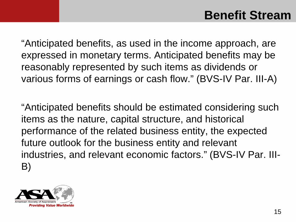
Benefit Stream
“Anticipated benefits, as used in the income approach, are expressed in monetary terms. Anticipated benefits may be reasonably represented by such items as dividends or various forms of earnings or cash flow.” (BVS-IV Par. III-A)
“Anticipated benefits should be estimated considering such items as the nature, capital structure, and historical performance of the related business entity, the expected future outlook for the business entity and relevant industries, and relevant economic factors.” (BVS-IV Par. III-B)
15
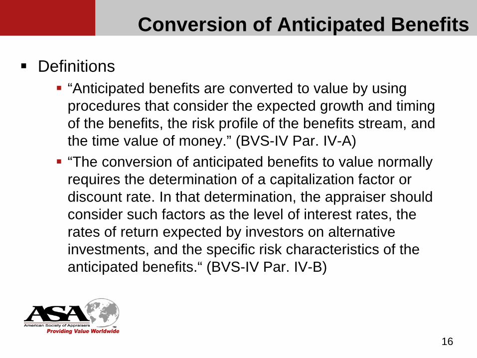
Conversion of Anticipated Benefits
Definitions “Anticipated benefits are converted to value by using
procedures that consider the expected growth and timing of the benefits, the risk profile of the benefits stream, and the time value of money.” (BVS-IV Par. IV-A) “The conversion of anticipated benefits to value normally
requires the determination of a capitalization factor or discount rate. In that determination, the appraiser should consider such factors as the level of interest rates, the rates of return expected by investors on alternative investments, and the specific risk characteristics of the anticipated benefits.“ (BVS-IV Par. IV-B)
16

Conversion of Anticipated Benefits
Consistency Between Discount Rate and Benefit Stream “The capitalization factors or discount rates should be
consistent with the types of anticipated benefits used.” (BVS-IV Par. IV-D) “For example, pre-tax factors or rates should be used
with pre-tax benefits; common equity factors or rates should be used with common equity benefits; and net cash flow factors or rates should be used with net cash flow benefits.” (BVS-IV Par. IV-D)
17
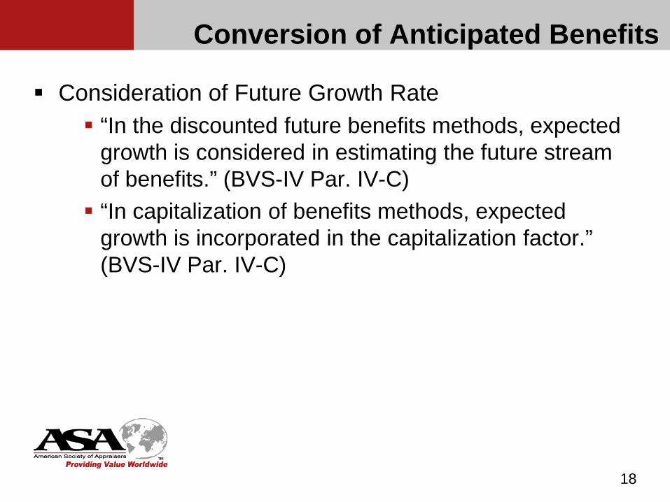
Conversion of Anticipated Benefits
Consideration of Future Growth Rate “In the discounted future benefits methods, expected
growth is considered in estimating the future stream of benefits.” (BVS-IV Par. IV-C) “In capitalization of benefits methods, expected
growth is incorporated in the capitalization factor.” (BVS-IV Par. IV-C)
18

Key Valuation Variables
19
Value (V) = Benefit Stream (BS)
Discount Rate (k) – Growth (g)

Chapter 3
Economic Benefits
20
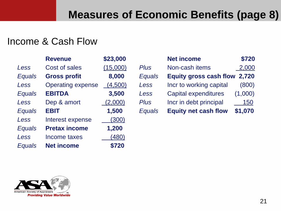
Measures of Economic Benefits (page 8)
Income & Cash Flow
21
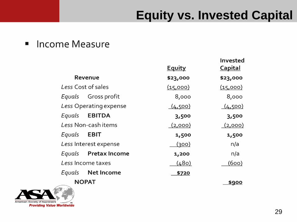
Revenue $23,000Less Cost of sales (15,000)Equals Gross profit 8,000Less Operating expense (4,500)Equals EBITDA 3,500Less Dep & amort (2,000)Equals EBIT 1,500Less Interest expense (300)Equals Pretax income 1,200Less Income taxes (480)Equals Net income $720
Net income $720Plus Non-cash items 2,000Equals Equity gross cash flow 2,720Less Incr to working capital (800)Less Capital expenditures (1,000)Plus Incr in debt principal 150Equals Equity net cash flow $1,070
Measures of Economic Benefits
Income vs. cash flow Cash-basis vs. accrual basis Different measures of income require different
discount or capitalization rates to yield the same value for the company.
22

Exercise 3-1
MEASURES OF ECONOMIC BENEFITS
Assume the following facts:Net Income = $800,000Depreciation = $350,000Interest expense = $100,000Capital expenditures = $250,000Increase in working capital = $75,000Increase in L-T debt = $200,000Tax rate = 40%
23
3-1(a) Calculate gross equity cash flow
3-1(b) Calculate net equity cash flow3-1(c) Calculate pre-tax income
Exercise 3-1 SOLUTION
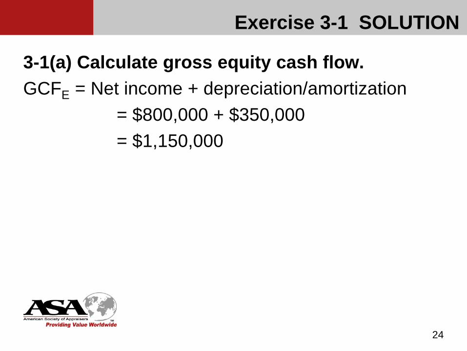
3-1(a) Calculate gross equity cash flow. GCFE = Net income + depreciation/amortization
= $800,000 + $350,000= $1,150,000
24
Exercise 3-1 SOLUTION
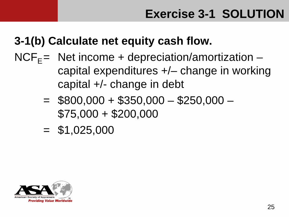
3-1(b) Calculate net equity cash flow. NCFE= Net income + depreciation/amortization –
capital expenditures +/– change in working capital +/- change in debt
= $800,000 + $350,000 – $250,000 –$75,000 + $200,000
= $1,025,000
25
Exercise 3-1 SOLUTION
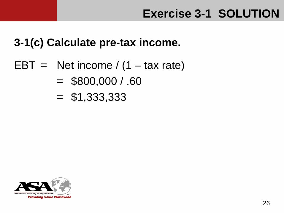
3-1(c) Calculate pre-tax income.
EBT = Net income / (1 – tax rate)= $800,000 / .60= $1,333,333
26

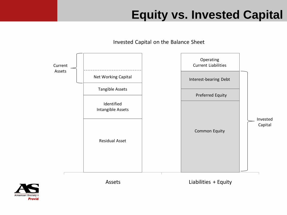
Equity vs. Invested Capital (page 11)
Matching the income measure with the subject interest Equity measures represent the returns available to the
equity holders Invested capital measures represent the returns
available to the equity holders and debt holders
27
28
Assets Liabilities + Equity
Net Working Capital
Tangible Assets
IdentifiedIntangible Assets
Residual Asset
OperatingCurrent Liabilities
Interest-bearing Debt
Preferred Equity
Common Equity
CurrentAssets
InvestedCapital
Invested Capital on the Balance Sheet
Equity vs. Invested Capital
29
Equity vs. Invested Capital
Net Cash Flow (page 12)
Net cash flow can also be determined on either an equity basis or an invested capital basis.
Equity net cash flow deducts interest expense on debt and adds or subtracts changes in debt principal. Cash flows that are paid to debt providers are excluded from the analysis, isolating the cash flow to equity only. An increase in debt is a cash inflow; a payment of debt is a cash outflow.
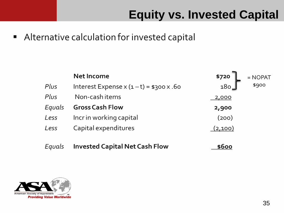
Invested capital net cash flow does not contain these two debt-related elements. Furthermore, income taxes are calculated on EBIT, which represents the earnings of the company prior to any payments to either debt or equity holders. In this way, the interest expense is becomes net of the tax benefit.
While the equity after tax income is referred to as Net Income, the invested capital after tax income is referred to as Net Operating Profit After Tax or “NOPAT”.
30

Defining Invested Capital Invested capital is the sum of equity and interest bearing debt in a
business enterprise. The debt is typically a) all interest-bearing debt or b) long-term interest-bearing debt.
Theoretically, invested capital debt includes interest-bearing debt used in the company’s long-term or permanent capital structure.
Note that as used above, “long-term” does not have the same meaning as “long-term debt” shown on the company’s balance sheet. It includes the short-term portion of long term debt as well.
Some companies (particularly small ones) may finance themselves “permanently” using only a revolving line of credit, credit cards, or short-term debt. In that case, in may be appropriate to include the revolving or short-term debt in invested capital, since, as a practical matter, it is treated by the company as long-term debt, and is unlikely to be paid down appreciably
31
It has become common practice to treat all interest-bearing debt as invested capital debt, with one major exception: Debt incurred on a temporary seasonal basis, which will be paid
off in the company’s normal cash cycle, is often treated as an operating liability of the company rather than invested capital debt.
In this case, interest expense associated with the temporary debt is treated as an operating expense and deducted from revenue in calculating invested capital net cash flow.
In any event, the interest expense associated with debt included in invested capital should not be deducted in the calculation of invested capital benefit streams.
32
Defining Invested Capital
Other exceptions may exist. For example, some analysts do not consider floor-plan debt and related interest for a car dealer to be invested capital since it is a routine aspect of dealership operations. The key factor is consistency between the treatment of the debt
principal and its related interest expense. If debt is treated as invested capital, do not deduct related interest
expense when calculating invested capital cash flow. If debt is treated as an operating item, related interest expense
should be deducted when calculating invested capital cash flow.
Any short-term debt (including the current portion of long-term debt) that is considered to be invested capital must be excluded from working capital calculations
33
Defining Invested Capital

Equity Cash Flow v IC Cash Flow
34
35
Equity vs. Invested Capital
Direct and indirect methods to value equity Direct: Applying discount and/or capitalization factors to
an equity benefit stream Indirect: Applying discount and/or capitalization factors
to an invested capital benefit stream, then subtracting the value of the debt in the invested capital
36
Equity vs. Invested Capital
Invested Capital
Defining invested capital (cont’d) Key is consistency: the interest expense for any debt
included in invested capital must be excluded from the determination of an invested capital income measure
Any short term debt included in invested capital must be excluded from operating working capital
37
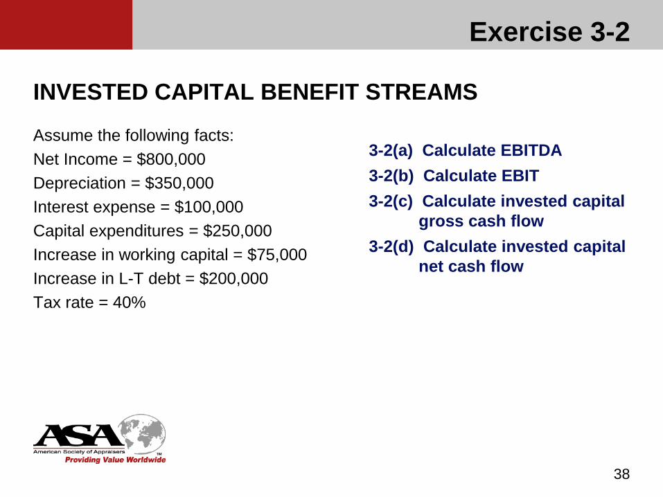
Exercise 3-2
INVESTED CAPITAL BENEFIT STREAMS
Assume the following facts:Net Income = $800,000Depreciation = $350,000Interest expense = $100,000Capital expenditures = $250,000Increase in working capital = $75,000Increase in L-T debt = $200,000Tax rate = 40%
38
3-2(a) Calculate EBITDA3-2(b) Calculate EBIT3-2(c) Calculate invested capital
gross cash flow3-2(d) Calculate invested capital
net cash flow
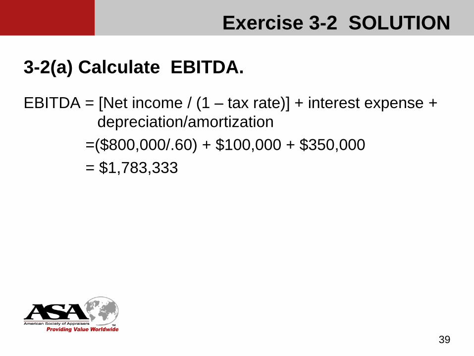
Exercise 3-2 SOLUTION
3-2(a) Calculate EBITDA.
EBITDA = [Net income / (1 – tax rate)] + interest expense + depreciation/amortization
=($800,000/.60) + $100,000 + $350,000= $1,783,333
39
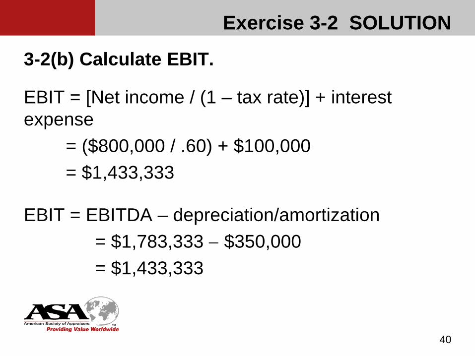
Exercise 3-2 SOLUTION
3-2(b) Calculate EBIT.
EBIT = [Net income / (1 – tax rate)] + interest expense
= ($800,000 / .60) + $100,000= $1,433,333
EBIT = EBITDA – depreciation/amortization= $1,783,333 − $350,000= $1,433,333
40

Exercise 3-2 SOLUTION
3-2(c) Calculate gross invested capital cash flow.
GCFIC = NOPAT + depreciation/amortization= [EBIT x (1 – tax rate)] + depreciation= ($1,433,333 x .60) + $350,000 = $860,000 + $350,000= $1,210,000
41

Exercise 3-2 SOLUTION
3-2(d) Calculate net invested capital cash flow.
NCFIC = NOPAT + depreciation/amortization – capital expenditures +/– change in working capital
=$860,000 + $350,000 – $250,000 – $75,000= $885,000
42
Equity vs. Invested Capital (page 17)
Application of discount and capitalization rates Equity measures should be discounted or capitalized
using an equity discount or capitalization factor (typically the cost of equity or equity multiples) Invested capital measures should be discounted or
capitalized using an invested capital discount or capitalization factor (typically the weighted average cost of capital or invested capital multiples)
43
Using the appropriate discount rate: Equity net cash flow is discounted using an equity
discount rate, which can be quantified using the buildup method, the capital asset pricing model (CAPM), or other methods. Equity discount rates are discussed in more detail later in this course.
Application of an equity discount rate and/or equity capitalization rate with an equity benefit stream results in the value of equity. This method is referred to as the direct-to-equity method.
44
Equity vs. Invested Capital

Invested capital cash flow is discounted using the weighted average cost of capital (WACC). WACC is a blend of an equity discount rate and a debt discount rate, based on an appropriate capital structure for the company.
Application of an invested capital discount rate and/or invested capital capitalization rate with an invested capital benefit stream results in the value of invested capital. The value of equity is obtained by subtracting the fair (market) value of outstanding debt as of the valuation date. This method is referred to as the indirect-to-equity method, because it first values invested capital, and equity can only be valued by then subtracting the value of debt.
45
Equity vs. Invested Capital

Matching Rate of Return to Benefit Stream
The best techniques for developing discount and capitalization rates result in rates that are directly applicable to net cash flow.
Discount rates and capitalization rates developed using the techniques presented in this course must be appropriately modified to apply to any other economic benefit.
In any event, the discount or capitalization rate used must be consistent with the economic benefit stream being uses (i.e., an after tax invested capital cash flow discount rate should be used on after tax invested capital cash flows, etc.);
46
For a particular business, there can be additional considerations in selecting an economic benefit stream to discount or capitalize: The nature and size of the business
Capital intensive, high debt/depreciation High growth – net income far different from net cf
The capital structure of the business1. Atypical debt/equity structure
The purpose of the appraisal1. Typically net cash flow for acquisitions2. Some legal jurisdictions prefer net income measures
The extent and quality of available information The particular interest being valued
1. Control v non-control
47
Matching Rate of Return to Benefit Stream

Exercise 3-3DETERMINING BENEFIT STREAMSUsing Exhibit 3-1 at the end of this chapter, calculate the following measures of 2011 income and indicate whether they are used to determine the value of equity or of invested capital:
48
Benefit MeasureCalculated
AmountEquity orInvested Capital?
Pretax income $EBITDA $Invested capital net cash flow $ Invested capitalNet operating profit after tax (NOPAT) $Equity net cash flow $ EquityNet income $Invested capital gross cash flow $ Invested cap[italEquity gross cash flow $ EquityEBIT $
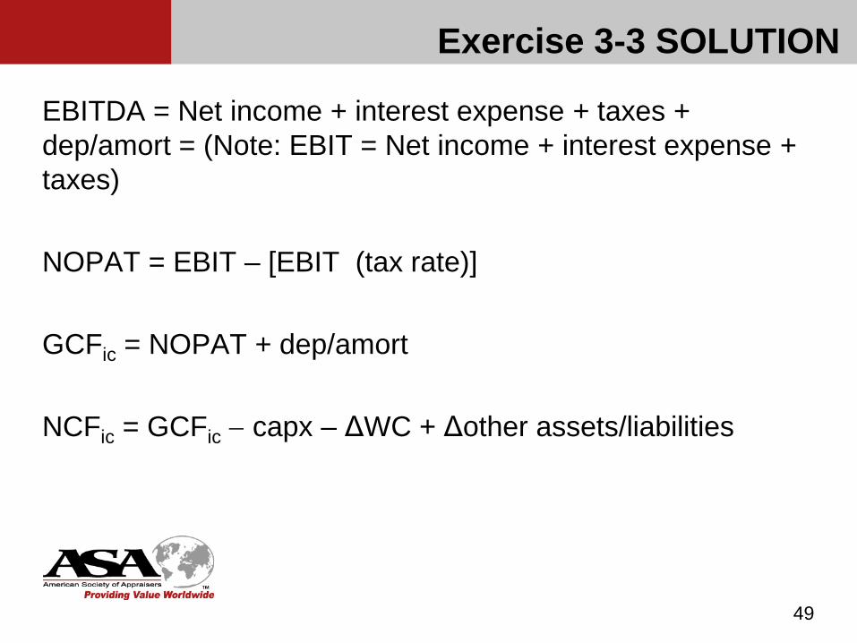
EBITDA = Net income + interest expense + taxes + dep/amort = (Note: EBIT = Net income + interest expense + taxes)
NOPAT = EBIT – [EBIT (tax rate)]
GCFic = NOPAT + dep/amort
NCFic = GCFic − capx – ΔWC + Δother assets/liabilities
49
Exercise 3-3 SOLUTION
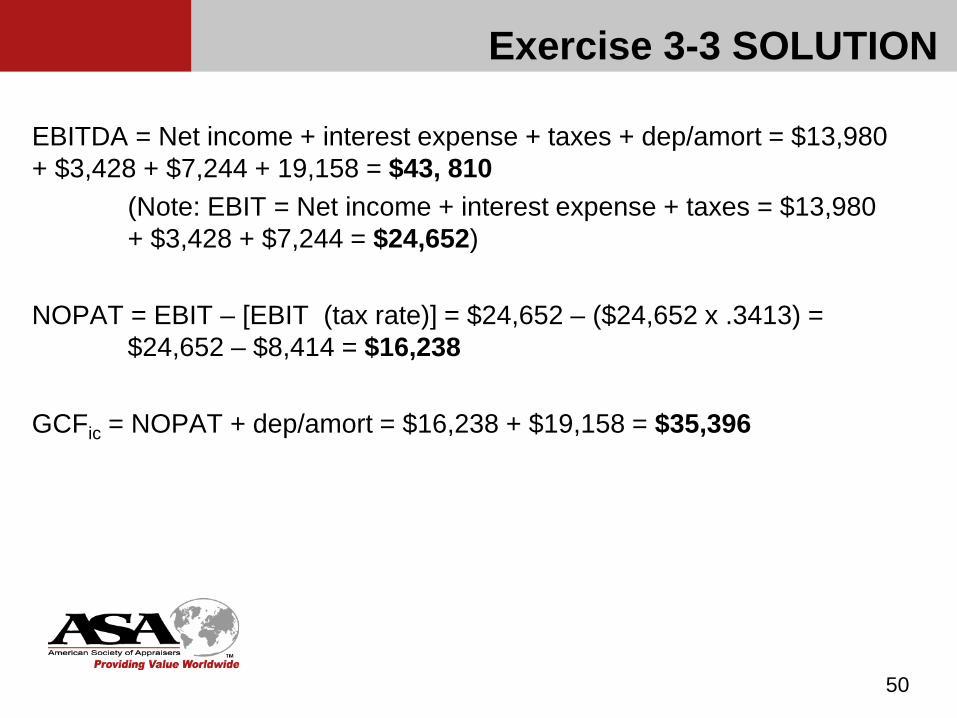
EBITDA = Net income + interest expense + taxes + dep/amort = $13,980 + $3,428 + $7,244 + 19,158 = $43, 810
(Note: EBIT = Net income + interest expense + taxes = $13,980 + $3,428 + $7,244 = $24,652)
NOPAT = EBIT – [EBIT (tax rate)] = $24,652 – ($24,652 x .3413) = $24,652 – $8,414 = $16,238
GCFic = NOPAT + dep/amort = $16,238 + $19,158 = $35,396
50
Exercise 3-3 SOLUTION
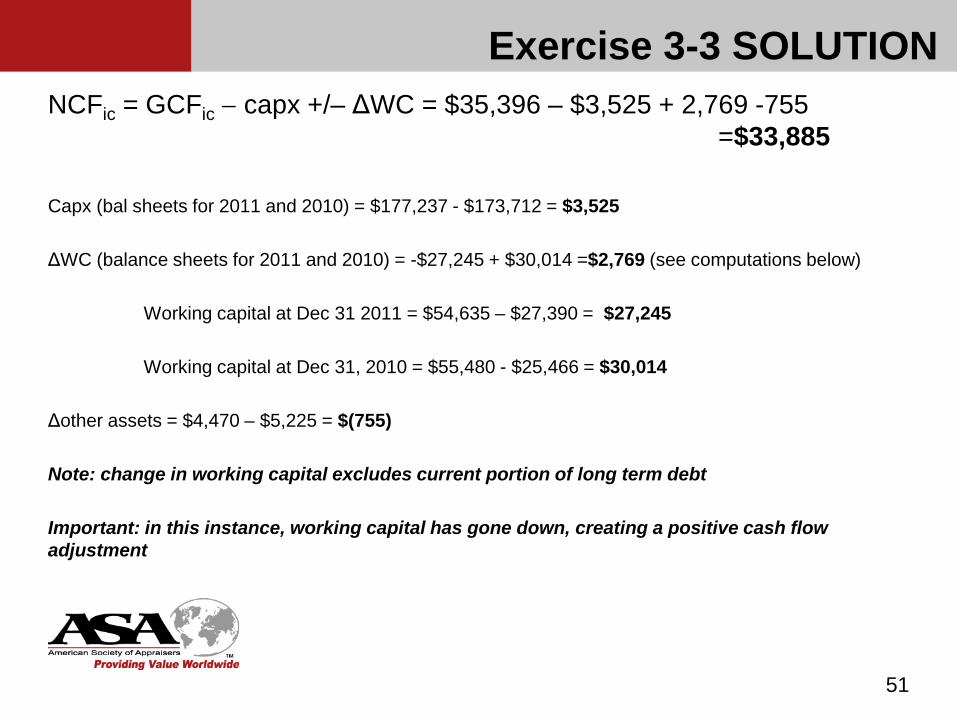
NCFic = GCFic − capx +/– ΔWC = $35,396 – $3,525 + 2,769 -755 =$33,885
Capx (bal sheets for 2011 and 2010) = $177,237 - $173,712 = $3,525
ΔWC (balance sheets for 2011 and 2010) = -$27,245 + $30,014 =$2,769 (see computations below)
Working capital at Dec 31 2011 = $54,635 – $27,390 = $27,245
Working capital at Dec 31, 2010 = $55,480 - $25,466 = $30,014
Δother assets = $4,470 – $5,225 = $(755)
Note: change in working capital excludes current portion of long term debt
Important: in this instance, working capital has gone down, creating a positive cash flow adjustment
51
Exercise 3-3 SOLUTION
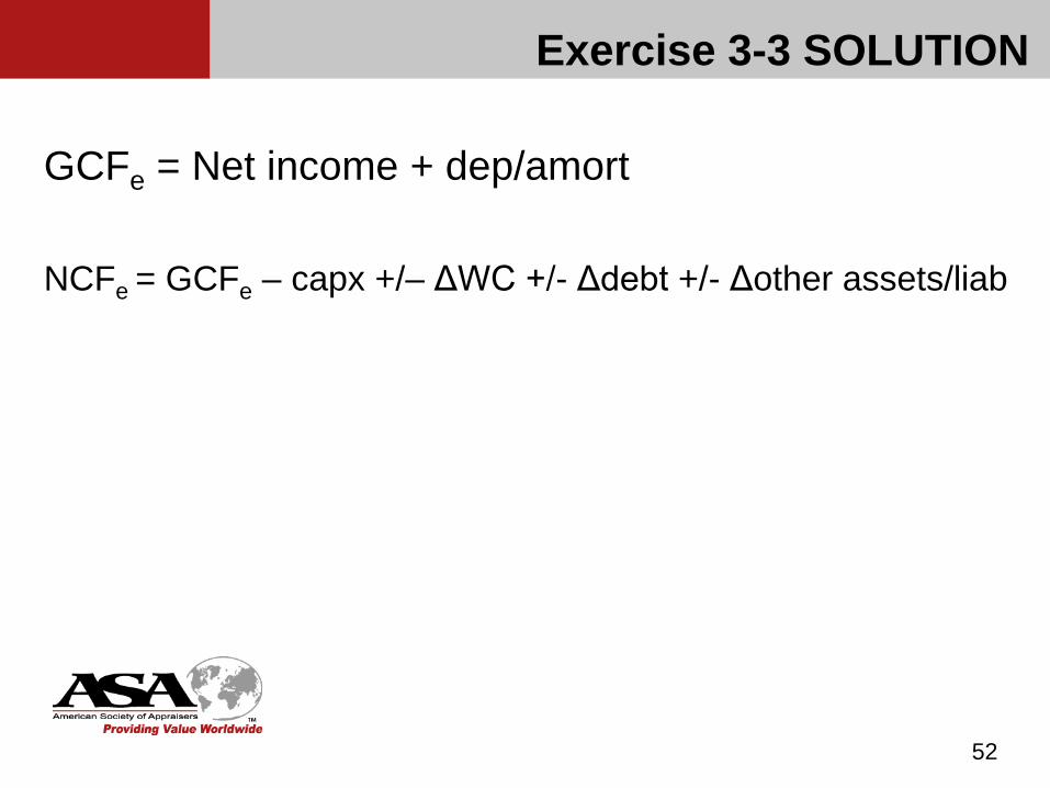
GCFe = Net income + dep/amort
NCFe = GCFe – capx +/– ΔWC +/- Δdebt +/- Δother assets/liab
52
Exercise 3-3 SOLUTION

GCFe = Net income + dep/amort = $13,980 + $19,158 = $33,138
NCFe = GCFe – capx +/– ΔWC +/- Δ other assets +/- Δdebt = $33,138 –$3,525 - $755 + $2,769 - $50 - $9,545 = $22,032
Δ other assets = $4,470 - $5,225=$(755)Δ long term debt= $33,574 - $43,119= $(9,545)Δ current portion of debt= $15,876 - $15,926= $(50)ΔWC (bal sheets ‘11 and ‘10) = $(11,369) + $14,088 = $2,719
Note that Δ current portion of debt of $(50) is either part of Δ long term debt or ΔWC
WC at Dec 31, 2011= $54,635 - $43,266=$11,369WC at Dec 31, 2010= $55,480 - $41,392=$14,088
53
Exercise 3-3 SOLUTION
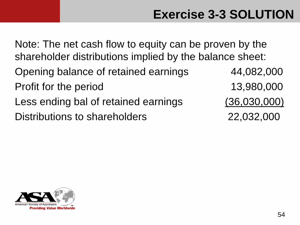
Note: The net cash flow to equity can be proven by the shareholder distributions implied by the balance sheet:Opening balance of retained earnings 44,082,000Profit for the period 13,980,000Less ending bal of retained earnings (36,030,000)Distributions to shareholders 22,032,000
54
Exercise 3-3 SOLUTION

55
Benefit MeasureCalculated
AmountEquity or
Invested Capital?
Pretax income $21,224 EquityEBITDA $43,810 Invested capitalInvested capital net cash flow $33,885 Invested capitalNet operating profit after tax (NOPAT) $16,238 Invested CapitalEquity net cash flow $22,032 EquityNet income $13,980 EquityInvested capital gross cash flow $35,396 Invested capitalEquity gross cash flow $33,138 EquityEBIT $24,652 Invested Capital
Exercise 3-3 SOLUTION
56
Equity InvestedCapital
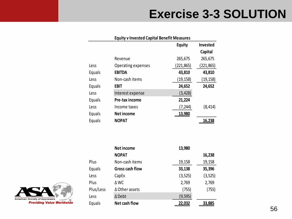
Revenue 265,675 265,675 Less Operating expenses (221,865) (221,865) Equals EBITDA 43,810 43,810 Less Non-cash items (19,158) (19,158) Equals EBIT 24,652 24,652 Less Interest expense (3,428) Equals Pre-tax income 21,224 Less Income taxes (7,244) (8,414) Equals Net income 13,980 Equals NOPAT 16,238
Net income 13,980 NOPAT 16,238
Plus Non-cash items 19,158 19,158 Equals Gross cash flow 33,138 35,396 Less CapEx (3,525) (3,525) Plus ∆ WC 2,769 2,769 Plus/Less ∆ Other assets (755) (755) Less ∆ Debt (9,595) Equals Net cash flow 22,032 33,885
Equity v Invested Capital Benefit Measures
Exercise 3-3 SOLUTION

Financial Statement Adjustments (p 21)Four reasons for potentially making adjustments to subject company financial statements:
1. To eliminate discretionary expenses of the business (e.g., above-market owner’s compensation, perquisites, related party transactions)
2. To make historical statements more representative of expected future performance: Eliminating or “smoothing” the effect of extraordinary and
nonrecurring items (Examples include casualty losses, discontinued operations, and legal settlements.)
Adjusting for a change in accounting conventions
3. To adjust for accounting methods used by the subject company that are not comparable to industry peers (for example, LIFO versus FIFO inventory accounting methods, accelerated depreciation methods, non-GAAP accounting methods)
4. To separate assets and liabilities (and related income and expense) that are not necessary for operating the business
57

Financial Statement Adjustments
Adjustments may be different for valuation of a minority interest versus a controlling interest.
One technique for valuing a minority interest is to discount or capitalize the economic benefit that is available to the minority interest shareholder. Fewer adjustments to the economic benefit may be necessary using this technique because minority
owners cannot typically affect or change policies set by the controlling owner. Typically, no adjustments are made for non-operating assets and liabilities, discretionary expenses
(including above-market owner compensation), and related party transactions. This is not a hard and fast rule and is dependent upon the facts and circumstances.
Adjustments may still be made for nonrecurring items and to match accounting methods used in the industry.
However, adjustments may be made if there is substantial reason to believe the controlling shareholders will make the associated changes in operations.
For an interest between 50% and 100%, adjustments will depend on the percentage held and on the level at which state law (or operating documents and contractual terms) accord the relevant powers of control
58
Typical areas to explore for possible normalizing adjustments can include, among others:
Owners’ salaries – salary surveys may provide evidence of market salaries for a particular job/position/title.If possible, it would be helpful to drill down in the data for salary levels by geography, years of experience, education level, etc.
Rent paid to related parties – where the property occupied by the company is owned by a related party, rent paid may be below or above market rates. If a recent real estate appraisal was done, it may offer insight into what the market rent for the property may be. If not, real estate professionals familiar with the market may be able to offer guidance on market rent for the property type in question.
– .
59
Financial Statement Adjustments
Consulting or fee arrangements with related parties –determine if services were provided by these individuals/entities, and if the amounts paid were appropriate in the circumstance.
Any other transaction that is not with an arm’s length partner.
60
Financial Statement Adjustments
Addressing the issue of synergies When employing the income approach, the analyst must
determine how to handle the potential incremental value from current or prospective synergies. Under the fair market value standard, the impact of
synergies is typically removed unless the current population of likely buyers includes mostly synergistic buyers. Similarly, under the fair value standard, the impact of
synergies is typically removed unless it is concluded that the current market participants could take advantage of, and pay for such synergies.
61
Financial Statement Adjustments
Financial Statement Adjustments
Adjusting for Non-operating Assets and Liabilities Identification of non-operating items
Operating assets and liabilities are considered essential to ongoing business operations. They are used to generate operating income.
Non-operating assets could be extracted from the business and sold separately without impairing operations.
Non-operating assets may be unrelated to business operations, or
They may be assets in “excess” of what is reasonable and necessary for operations.
In either case, they have a different level of risk and required return than business operations, which justifies treating them differently.
62
Financial Statement Adjustments
Non-operating liabilities May be associated with a non-operating asset Another common non-operating liability in small
businesses is a shareholder loan that is essential to support the business and cannot be repaid without endangering its survival. This is not a true liability, but a disguised form of equity.
63

Financial Statement Adjustments
When valuing a control interest, non-operating assets and liabilities and their related income or expense are usually separated from the analysis of the operating business. Remove non-operating assets and liabilities from the operating balance
sheet. Carefully identify associated income and expense and remove it from
the operating income statement. Determine the fair market value of non-operating assets and liabilities,
which may reflect taxes and transactions costs related to a sale of these items.
Add the fair market value of the non-operating items to the value of operations to obtain the total value of the business.
Note that the opposite of an excess asset is an asset deficiency, such as deficient working capital or inadequate or aged production capacity (fixed assets). In this case, the amount of the deficiency may be subtracted from the value of the business.
64

Exercise 3-4Using Exhibit 3-1 at the end of this chapter, determine if a normalizing adjustment is needed for each of the following for 2011 and, if so, how would you determine the amount of the adjustment. Assume you are valuing a controlling interest.
1. Other salaries and fringes include compensation for two of the CEO’s family members who work part time, but receive compensation based on full time salaries.
2. Professional fees and consulting expense includes legal fees of $75,000 for the negotiation of the buyout of a former shareholder.
3. Rent and storage includes below market rent for a facility owned by a non-related entity, with one year left on the lease.
4. Interest expense includes a fee paid to the majority shareholder to compensate her for providing a personal guarantee on a $1,000,000 line of credit, in order to secure a lower interest rate from the lender.
65

Exercise 3-4 SolutionOther salaries and fringes include compensation for two of the CEO’s family members who work part time, but receive compensation based on full time salaries.
Salaries expense should be reduced by the amount by which the compensation paid exceeds the market value of the services paid.
66

Exercise 3-4 SolutionProfessional fees and consulting expense includes legal fees of $75,000 for the negotiation of the buyout of a former shareholder.
The analyst needs to explore whether this is something that occurs periodically, or is a non-recurring expense that cannot be expected to recur in the future. If it is not uncommon, it probably should not be an adjustment.
67
Exercise 3-4 SolutionRent and storage includes below market rent for a facility owned by a non-related entity, with one year left on the lease.
This is not an item that should be adjusted, since the arrangement is with an independent party and is the result of an arm’s length arrangement.However, since there is one year left on the lease, the analyst needs to consider if the lease renewal will be at the higher market level or, alternatively, if the company will move to a different location altogether, and what the rent might be at that location.
68
Exercise 3-4 SolutionInterest expense includes a fee paid to the majority shareholder to compensate her for providing a personal guarantee on a $1,000,000 line of credit, in order to secure a lower interest rate from the lender.
The analyst should determine what the effective interest rate paid by the company is with and without the fee paid to the shareholder, and assess whether the fee is excessive or insufficient, in the circumstances.
69
Chapter 4
Projecting Financial Statements
70
Sources of projections (page 28)
Management—many companies prepare internal financial statement projections for banking and managerial purposes. These should be included as an item in the document request. If management’s projections are used, the variables must be vetted based
upon the appraiser’s training, experience and independent research and on the accuracy of management’s prior projections.
Management’s projections should be analyzed for ulterior motives:
How to deal with management-prepared projections that lack credibility
Practitioner—if the subject company does not prepare projections, the appraiser may consider either working with management to prepare projections or independently preparing a projection.
71

Projections can be a weighted average or a simple average of prior years’ operations, or the prior year amount grown by a certain amount. Using an average of prior results for a company that is experiencing growth will tend to understate value.
If a company is growing, then by definition any average of prior results, even a weighted average giving great weight to the most recent period, will yield a number that is below what should be expected.
72
Sources of projections

Projections
For example, the following revenue pattern shows annual growth of 5%.
If the company is growing by 5%, 20X6 revenues should be $1,276,281. Any average of the prior years will result in an estimate of revenues that is too low.
73
20X1 20X2 20X3 20X4 20X5Revenues 1,000,000 1,050,000 1,102,500 1,157,625 1,215,506
Projections should be developed line by line, and not in large subgroups (i.e., cost of goods as a single number) so that a thoughtful examination of the details of the balance sheet and income statement accounts is not lost.
74
Projections

The projections should be reviewed for various financial relationships, including- Working capital balances are maintained at the
appropriate levels, both in dollar amounts and in terms of ratios such as working capital, receivables/inventory turnover, etc.
Capital expenditures take into account recent amounts of cap ex or the deferral of cap ex, and whether cap ex will be paid for out of cash flow or be financed
75
Projections
Debt service, and its impact on interest expense, must be considered in the context of the amortization of installment loans, the need for additional borrowing, or the presence, and limits, of lines of credit
76
Projections
Factors to Consider (page 29)
Macroeconomic Factors Industry Factors Local Economic Factors Company Factors Income Statement considerations Balance sheet considerations
77

Methods of Projecting Percent of Sales Projections Assumes that certain expenses, assets, and liabilities maintain a
constant relationship with sales Most common methodology Easy to implement Can be implemented based on past company and/or industry
performance. May not be appropriate for start-up companies (most commonly used for mature companies)
Monte Carlo Simulations More complex—large number of variables Often requires specialized software
Probability-Weighted Models (best case, expected case, worst case)
78
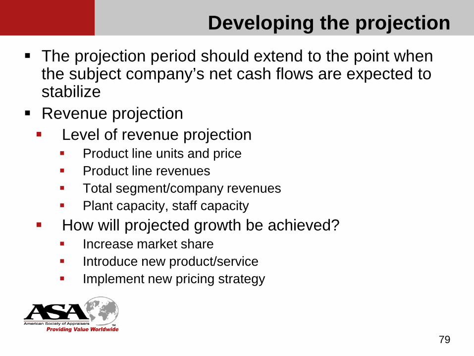
Developing the projection The projection period should extend to the point when
the subject company’s net cash flows are expected to stabilize
Revenue projection Level of revenue projection
Product line units and price Product line revenues Total segment/company revenues Plant capacity, staff capacity
How will projected growth be achieved? Increase market share Introduce new product/service Implement new pricing strategy
79

Developing the projection Historical growth as a basis for future growth
Growth projections should be forward looking. However, historical growth can be informative
Measures of historical growth Average annual growth - Susceptible to volatility Compounded annual growth CAGR will always be lower than the annual average growth
except when the year-to-year growth is the same over the entire period
CAGR ignores what happens in the interim years Median annual growth May not discern trends
Log linear regression Incorporates information from all years
80

Developing the projection Expense projection Determination of variable, semi-variable, and fixed
expenses: Look at the historical percent of sales, or cost per unit
produced/sold, for expense line items; consistent percent of sales or dollar per unit may suggest the expense is variable and dependent on revenues. Determine the extent of correlation between revenues
(or units) and the expense item. A high correlation may suggest the expense is variable and dependent on revenues. Discuss the expense categories with management.
81
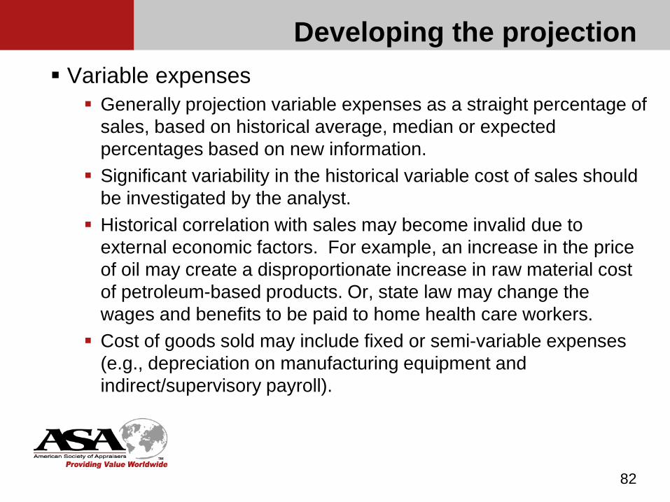
Developing the projection Variable expenses
Generally projection variable expenses as a straight percentage of sales, based on historical average, median or expected percentages based on new information.
Significant variability in the historical variable cost of sales should be investigated by the analyst.
Historical correlation with sales may become invalid due to external economic factors. For example, an increase in the price of oil may create a disproportionate increase in raw material cost of petroleum-based products. Or, state law may change the wages and benefits to be paid to home health care workers.
Cost of goods sold may include fixed or semi-variable expenses (e.g., depreciation on manufacturing equipment and indirect/supervisory payroll).
82

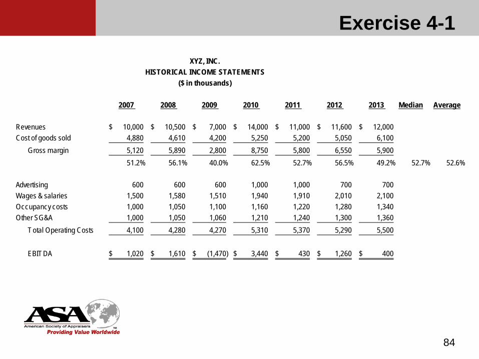
Exercise 4-1
83
PROJECTING GROSS MARGINPlease refer to the income statements for XYZ, Inc. in Exhibit 4-1 at the end of this chapter.
4-1(i) What COGS% would you use for your 2014 projection and why?
4-1(ii) What possible conclusions, if any, could you draw from this historical experience? What questions would you raise in your site visit and management interview?
Exercise 4-1
84
2007 2008 2009 2010 2011 2012 2013 Median Average
Revenues 10,000$ 10,500$ 7,000$ 14,000$ 11,000$ 11,600$ 12,000$ Cost of goods sold 4,880 4,610 4,200 5,250 5,200 5,050 6,100
Gross margin 5,120 5,890 2,800 8,750 5,800 6,550 5,900 51.2% 56.1% 40.0% 62.5% 52.7% 56.5% 49.2% 52.7% 52.6%
Advertising 600 600 600 1,000 1,000 700 700 Wages & salaries 1,500 1,580 1,510 1,940 1,910 2,010 2,100 Occupancy costs 1,000 1,050 1,100 1,160 1,220 1,280 1,340 Other SG&A 1,000 1,050 1,060 1,210 1,240 1,300 1,360
Total Operating Costs 4,100 4,280 4,270 5,310 5,370 5,290 5,500
EBITDA 1,020$ 1,610$ (1,470)$ 3,440$ 430$ 1,260$ 400$
XYZ, INC.HISTORICAL INCOME STATEMENTS
($ in thousands)
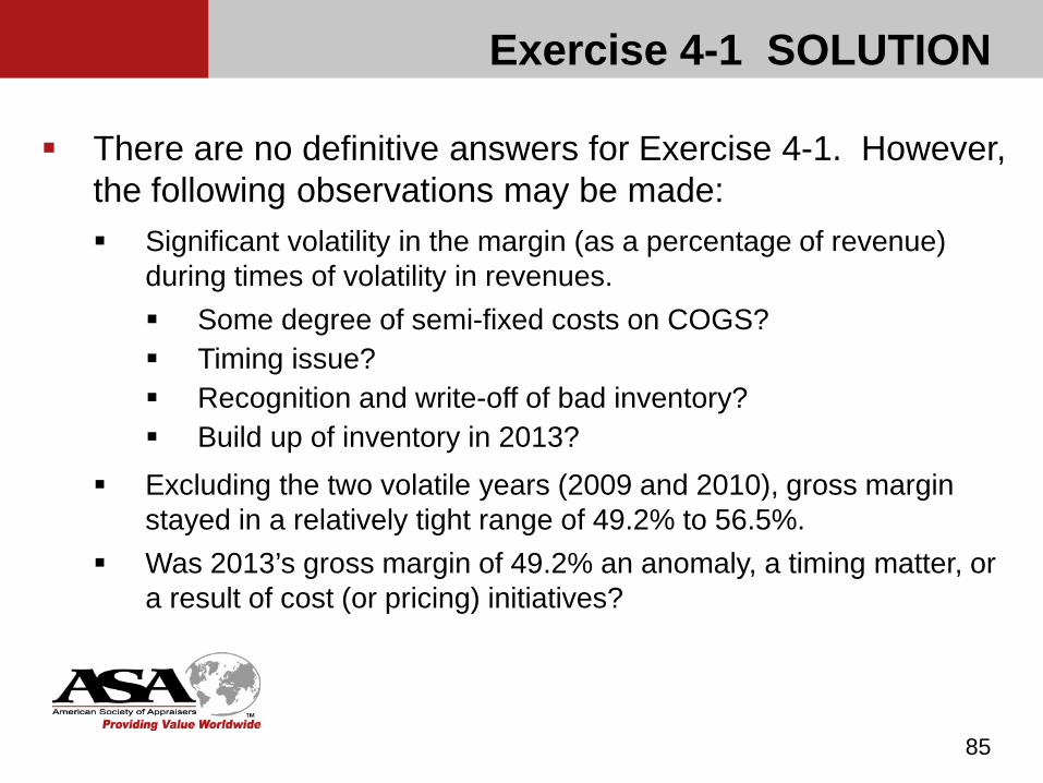
Exercise 4-1 SOLUTION
85
There are no definitive answers for Exercise 4-1. However, the following observations may be made: Significant volatility in the margin (as a percentage of revenue)
during times of volatility in revenues. Some degree of semi-fixed costs on COGS? Timing issue? Recognition and write-off of bad inventory? Build up of inventory in 2013?
Excluding the two volatile years (2009 and 2010), gross margin stayed in a relatively tight range of 49.2% to 56.5%.
Was 2013’s gross margin of 49.2% an anomaly, a timing matter, or a result of cost (or pricing) initiatives?
Exercise 4-2
86
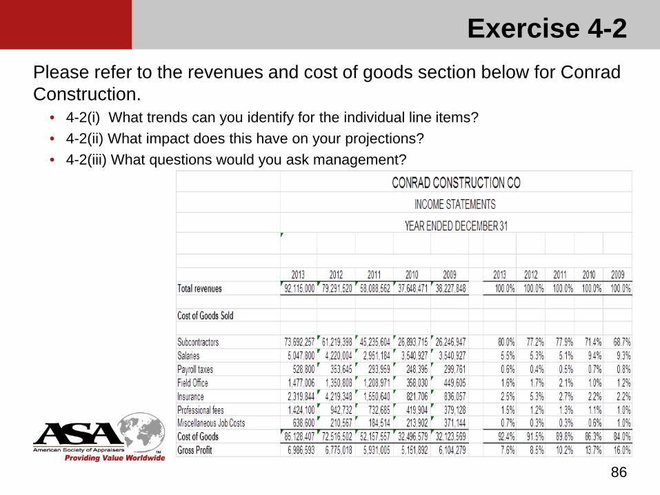
Please refer to the revenues and cost of goods section below for Conrad Construction.
• 4-2(i) What trends can you identify for the individual line items?• 4-2(ii) What impact does this have on your projections?• 4-2(iii) What questions would you ask management?
Exercise 4-2 SOLUTION As before, there are no definitive answers for Exercise 4-2.
However, the following observations may be made:
As revenues have grown, subcontractors have grown as a % of revenues
After 2010, the dollar amount of Field Office expense seems to be fairly fixed
Insurance was unusually high in 2012, perhaps due to a one-time charge, or possibly an acceleration of 2012 expenses. These two possible explanations (and others) could lead to very different projection assumptions.
87
Developing the projection
Fixed/semi-fixed expenses Salaries & wages Occupancy costs Interest expense projected as a function of debt levels and
projected capital structure (Interest expense may be plugged at first and fine-tuned later since exact debt level is unknown.)
Taxes based on projected effective tax rate of the subject company. Any NOLs must be dealt with
Other items of expense and income must be projected individually.
Remember, fixed costs are only valid within relevant ranges of production and sales.
88
Taxing Pass-Through Entities
The rates of return used in the income approach are derived from the public marketplace, which is almost exclusively made up of C corporations. For purposes of BV202 it is assumed the subject company is also a C corporation; the subject company is thus comparable to the companies from which the discount rate is derived, at least as it relates to corporate level taxes.
Often, we are asked to value an interest in a pass-through entity (“PTE”) such as a Subchapter S corporation, partnership or LLC. Such an entity is considered a pass-through entity because its income is not taxed at the entity level, but rather is taxed to the owner on the owner’s personal income tax return.
A detailed discussion of the valuation considerations surrounding this topic is reserved for BV204. However, a summary of the rationale for treating a PTE as though it were a C corporation, for valuation purposes, is presented below.
89
Taxing Pass-Through Entities
It is the owner of a pass-through entity that is liable for tax on his or her pro rata portion of the company’s earnings, but at personal income tax rates. Thus, the owner is required to pay a tax based on the amount of company income.
The cash to pay this tax must come either from the owner’s personal assets or from cash distributions from the company. In either case, it is assumed the working capital and cash balances of the company will not be impaired, but will be maintained at an appropriate level to adequately fund operations. If the owner of a pass-through entity pays the tax out of personal assets, the company usually makes distributions sufficient at least to cover the tax payment, so that the owner is cash neutral as it relates to taxes on the company’s income. Thus, the net economic impact of the taxes on the owner is the same as if the company paid the tax.
90
Taxing Pass-Through Entities
For these reasons, for valuation purposes the shareholders’ pass-through of S corporation earnings, and their accompanying payment of taxes on those corporate earnings is indeed a ‘corporate tax’ which is economically equivalent to the corporate tax paid by C corporations.
For valuation purposes, appraisers should consider this tax liability as real at the corporate level.” (Chris Mercer, Valuing Shareholder Cash Flows, 2005 E-Book Edition, Peabody Publishing, LP, Memphis, Tennessee, 2005, page 132, emphasis in the original.)
91
Exercise 4-3Please refer to the income statements for GDT, Inc. in Exhibit 4-6 at the end of this chapter. Assume the following:
- Revenues will increase 10% and 15% in years 2012 and 2013 respectively.- Approximately 75% of all Salaries and Fringe Benefits are fixed and will grow at 5% per
year. The remaining 25% of Salaries and Fringe Benefits are variable and will grow at the same rate as Revenues.
- Approximately 60% of Purchased Transportation are fixed and will grow at 5% per year. - The remaining 40% of Salaries and Wages are variable and will grow at the same rate as
Revenues.- Rent and Storage costs will grow at 5% per year.- Approximately 90% of all other expenses are fixed and will grow at 5% per year. The
remaining 10% of all other expenses are variable and will grow at the same rate as Revenues.
- Generate an operating expense projection for 2012 and 2013. Assume the subject interest lacks control. Be prepared to explain and support the bases for your projections.
92
Exercise 4-3 Solution
Drivers’ salaries and fringes 2012 Drivers’ salaries and fringes = (2011 Drivers’ salaries and
fringes 75% 1.05) + (2011 Drivers’ salaries and fringes 25% 1.10) = ($92,035,450 75% 1.05) + ($92,035,450 25% 1.10) = $72,477,917 + $25,309,749 = $97,787,666
2013 Drivers’ salaries and fringes = (2012 Drivers’ salaries and fringes 75% 1.05) + (2012 Drivers’ salaries and fringes 25% 1.15) = ($97,787,666 75% 1.05) + ($97,787,666 25% 1.15) = $77,007,787 + $28,113,954 = $105,121,741
The other salaries and fringes amounts are computed in the same manner
93
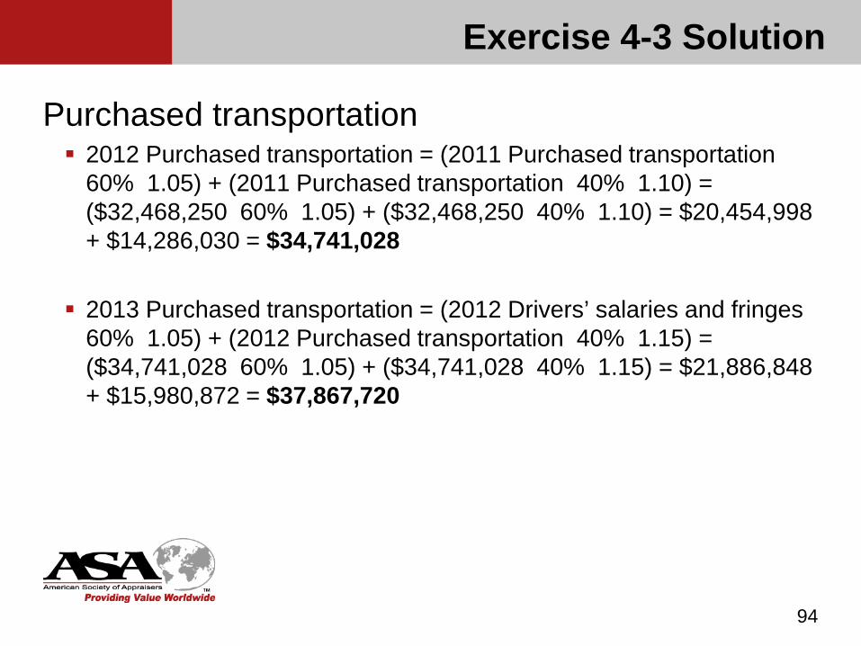
Exercise 4-3 Solution
Purchased transportation 2012 Purchased transportation = (2011 Purchased transportation
60% 1.05) + (2011 Purchased transportation 40% 1.10) = ($32,468,250 60% 1.05) + ($32,468,250 40% 1.10) = $20,454,998 + $14,286,030 = $34,741,028
2013 Purchased transportation = (2012 Drivers’ salaries and fringes 60% 1.05) + (2012 Purchased transportation 40% 1.15) = ($34,741,028 60% 1.05) + ($34,741,028 40% 1.15) = $21,886,848 + $15,980,872 = $37,867,720
94

Transportation rental 2012 Transportation rental = (2011 Transportation rental 90% 1.05)
+ (2011 Transportation rental 10% 1.10) = ($10,822,750 90% 1.05) + ($10,822,750 10% 1.10) = $10,227,499 + $1,190,502 = $11,418,001
2013 Transportation rental = (2012 Transportation rental 90% 1.05) + (2012 Transportation rental 10% 1.15) = ($11,418,001 90% 1.05) + ($11,418,001 10% 1.15) = $10,790,011 + $1,313,070 = $12,103,081
All the other expense items, other than rent and stage are computed in the same manner
95
Exercise 4-3 Solution
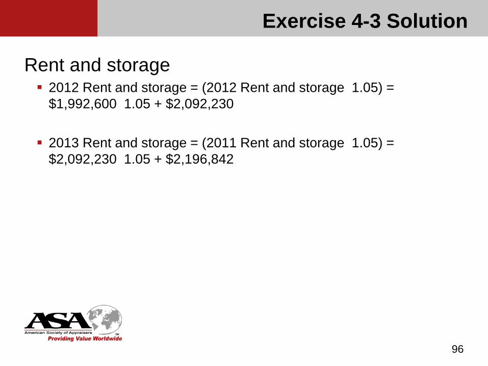
Rent and storage 2012 Rent and storage = (2012 Rent and storage 1.05) =
$1,992,600 1.05 + $2,092,230
2013 Rent and storage = (2011 Rent and storage 1.05) = $2,092,230 1.05 + $2,196,842
96
Exercise 4-3 Solution

97
2011 2012 2013Total revenues 265,675,000 292,242,500 336,078,875
Operating expensesDrivers' salaries and fringes 92,035,450 97,787,666 105,121,741 Other salaries and fringes 16,241,550 17,256,647 18,550,895 Officers' salaries and fringes 9,250,000 9,828,125 10,565,234 Purchased transportation 32,468,250 34,741,028 37,867,720 Transportation rental 10,822,750 11,418,001 12,103,081 Fuel 21,315,900 22,488,275 23,837,571 Rent and storage 1,992,600 2,092,230 2,196,842 Insurance - general 3,985,100 4,204,281 4,456,537 Licenses and fees 2,656,800 2,802,924 2,971,099 Repairs and maintenance 5,313,500 5,605,743 5,942,087 Other operating supplies 7,970,100 8,408,456 8,912,963 Pension, profit-sharing 3,985,100 4,204,281 4,456,537 Telephone 1,992,600 2,102,193 2,228,325 Computers and technology 1,594,100 1,681,776 1,782,682 Utilities 4,250,800 4,484,594 4,753,670 Insurance - group 2,656,800 2,802,924 2,971,099 Insurance - other 106,300 112,147 118,875 Professional fees and consulting 132,800 140,104 148,510 Advertising 797,000 840,835 891,285 Other general and admin 2,297,500 2,423,863 2,569,294
221,865,000 235,426,093 252,446,047
Operating income 43,810,000 56,816,407 83,632,828
GENERAL DELIVERY TRUCKING, INCEXERCISE SOLUTION
Exercise 4-3 Solution

Developing the projection (page 40)
Working capital Project working capital components based on relationship with revenue
or expense categories Cash-cash expenses-cash turnover
A/R-credit sales-days of sales or A/R turnover
Inventory-COGS-days of COGS or inventory turnover
A/P-total expenses (excl. payroll)-days of expenses or A/P turnover
Accrued taxes, payroll, other expenses
98
Best to project each component of working capital separately as opposed to projecting net working capital as one variable. If working capital is projected as a single variable, the appraiser may not become aware of underlying assumptions that are unreasonable or unsustainable, such as inventory turnover or days receivables that are too high or too low
99
Developing the projection
100
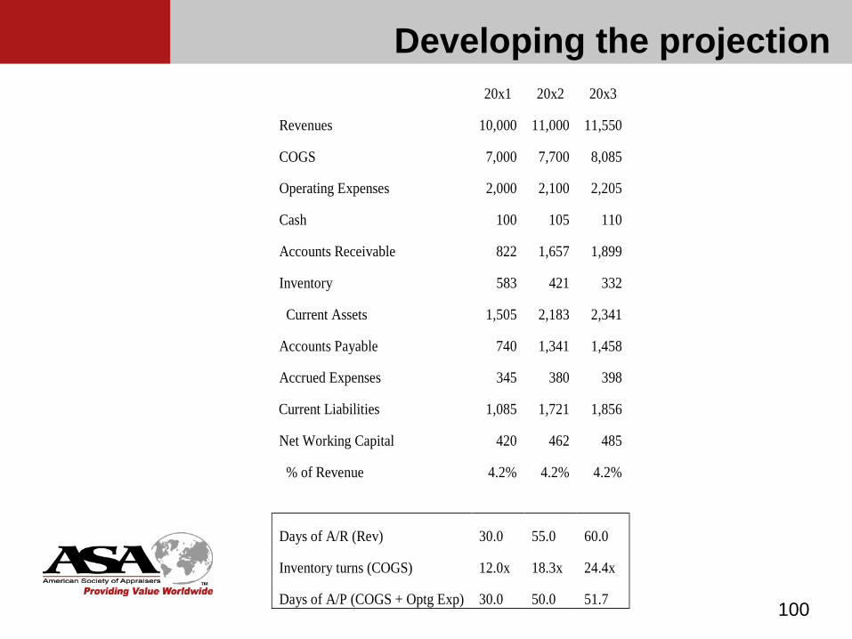
20x1 20x2 20x3
Revenues 10,000 11,000 11,550
COGS 7,000 7,700 8,085
Operating Expenses 2,000 2,100 2,205
Cash 100 105 110
Accounts Receivable
Inventory
822
583
1,657
421
1,899
332
Current Assets 1,505 2,183 2,341
Accounts Payable 740 1,341 1,458
Accrued Expenses 345 380 398
Current Liabilities 1,085 1,721 1,856
Net Working Capital 420 462 485
% of Revenue 4.2% 4.2% 4.2%
Days of A/R (Rev) 30.0 55.0 60.0
Inventory turns (COGS) 12.0x 18.3x 24.4x
Days of A/P (COGS + Optg Exp) 30.0 50.0 51.7
Developing the projection

101
PROJECTING NET WORKING CAPITALPlease refer to the income statements for XYZ, Inc. in Exhibit 4-1 at the end of this chapter. Assume the following: Revenues will grow by 10% in 2014 and 15% in 2015 Gross margins for 2014 and 2015 will be 53% Management advises it intends to implement the following strategies in 2014 (consider whether, given the company’s historical trends these goals can be achieved, and if you feel you must modify them in any way):
A minimum cash balance of $50 will be kept to fund operating needs. An aggressive plan to reduce days of accounts receivables outstanding to 15 days. Just-in-time inventory system to increase turns to 9 times. Making sure vendors are paid within 30 days.
The long term debt is scheduled to have $250 of principal repayment in 2014 and in 2015. Accrued expenses are expected to be $82 as of 12/31/14 and $91 as of 12/31/15. Wages and salaries expense will grow by 5% in both 2014 and 2015, and accrued payroll is expected to be eight days for both years
Exercise 4-4A

Exercise 4-4A (cont’d)
102
PROJECTING NET WORKING CAPITALGenerate an operating net working capital projection for 2014 and 2015. Assume the subject interest lacks control. Be prepared to explain and support the bases for your projections.

Exercise 4-4A SOLUTION
103
Cash projection2014 cash = $50 (given)2015 cash = $50 (given)Any additional cash flow is assumed to be distributed.

Exercise 4-4A SOLUTION
104
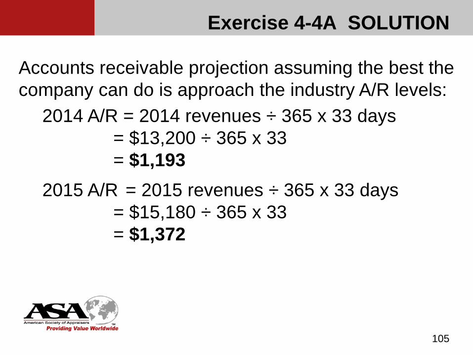
Accounts receivable projection Management wants to reduce outstanding A/R to 15 days. Historically, days of A/R have ranged from 40 to 60, while the industry
has been fairly stable at around 33. Will management be successful in reducing A/R balances to the levels
desired in light of its own history and that of the industry? Will additional cost and/or price discounts be necessary to do so? The point is that just because management wants to reduce A/R
does not mean that it will be able to do so. It is the analyst’s job to determine if this goal is reasonable.
For purposes of this exercise, the industry average of 33 days is used
Exercise 4-4A SOLUTION
105
Accounts receivable projection assuming the best the company can do is approach the industry A/R levels:
2014 A/R = 2014 revenues ÷ 365 x 33 days= $13,200 ÷ 365 x 33 = $1,193
2015 A/R = 2015 revenues ÷ 365 x 33 days = $15,180 ÷ 365 x 33 = $1,372
Exercise 4-4A SOLUTION
106
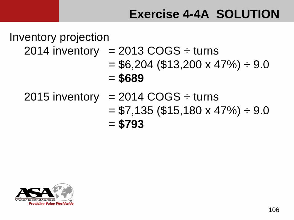
Inventory projection2014 inventory = 2013 COGS ÷ turns
= $6,204 ($13,200 x 47%) ÷ 9.0 = $689
2015 inventory = 2014 COGS ÷ turns = $7,135 ($15,180 x 47%) ÷ 9.0 = $793

Exercise 4-4A SOLUTION
107
Accounts payable projection2014 A/P = 2009 COGS / 365 x 30
= $6,204 / 365 x 30= $510
2015 A/P = 2010 COGS / 365 x 30= $7,135 / 365 x 30= $586

Exercise 4-4A SOLUTION
108
Current portion of long-term debt projection:This is part of the invested capital of the company and, therefore, not included in operating working capital.

Exercise 4-4A SOLUTION
109
Accrued expenses projection2014 acc’d exp = $82 (given)2015 acc’d exp = $91 (given)
Exercise 4-4A SOLUTION
110
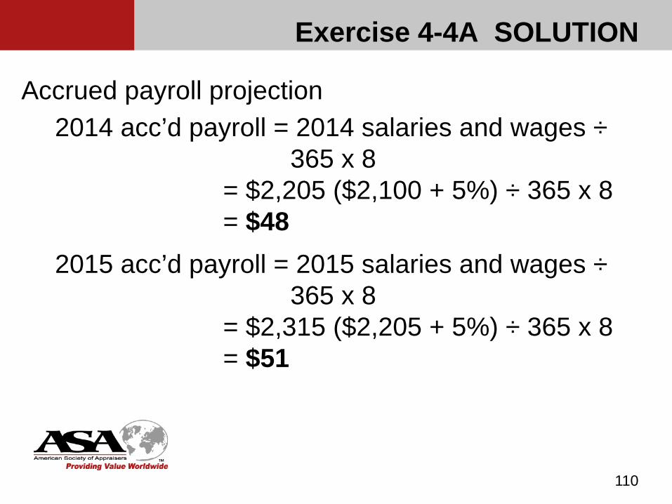
Accrued payroll projection2014 acc’d payroll = 2014 salaries and wages ÷
365 x 8 = $2,205 ($2,100 + 5%) ÷ 365 x 8 = $48
2015 acc’d payroll = 2015 salaries and wages ÷365 x 8
= $2,315 ($2,205 + 5%) ÷ 365 x 8 = $51

Exercise 4-4A SOLUTION
111
2014 and 2015 Projected Operating Net Working Capital2013
Actual2014
projection2015
projection
Current assetsCash 20 50 50Accounts receivable 1,320 1,193 1,372Inventory 950 689 793Total current assets 2,290 1,932 2,215
Current liabilitiesAccounts payable 1,040 510 586Accrued expenses 80 82 91Accrued payroll 50 48 51Total current liabilities 1,170 640 728
Net working capital 1,120 1,292 1,487
% of revenues 9.3% 9.8% 9.8%Change in NWC n/a +172 +195

Developing the projection (page 43)
Fixed assets Should consider need to replace existing assets and need to
expand to meet growth expectations Historical relationship between capex needs and revenues
may provide a reasonable basis Relationship between Projected capex and Projected
depreciation requires reconciliation
112
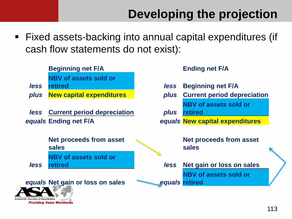
Developing the projection
Fixed assets-backing into annual capital expenditures (if cash flow statements do not exist):
113
Beginning net F/A Ending net F/A
lessNBV of assets sold or retired less Beginning net F/A
plus New capital expenditures plus Current period depreciation
less Current period depreciation plusNBV of assets sold or retired
equals Ending net F/A equals New capital expenditures
Net proceeds from asset sales
Net proceeds from asset sales
lessNBV of assets sold or retired less Net gain or loss on sales
equals Net gain or loss on sales equalsNBV of assets sold or retired

Developing the projection
Debt/financing projection Should consider existing capital structure and source(s) of
capital for growth Operating debt (e.g., line of credit) may be required to fund
cash flow deficits Interest projection should be consistent with debt projection
114
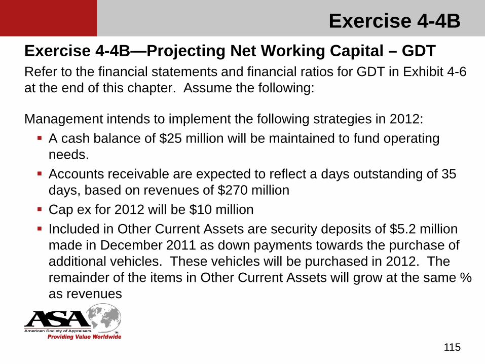
Exercise 4-4BExercise 4-4B—Projecting Net Working Capital – GDTRefer to the financial statements and financial ratios for GDT in Exhibit 4-6 at the end of this chapter. Assume the following:
Management intends to implement the following strategies in 2012: A cash balance of $25 million will be maintained to fund operating
needs. Accounts receivable are expected to reflect a days outstanding of 35
days, based on revenues of $270 million Cap ex for 2012 will be $10 million Included in Other Current Assets are security deposits of $5.2 million
made in December 2011 as down payments towards the purchase of additional vehicles. These vehicles will be purchased in 2012. The remainder of the items in Other Current Assets will grow at the same % as revenues
115
Exercise 4-4B
Assumptions, continued: Certain fixed asset loans are coming due in 2013 so that the current
portion of long term debt at the end of 2012 will be $16,450,000 Accounts payable, accruals and accrued expenses will be managed
so that a current ratio of 1.2:1 will be maintained
Prepare the current asset and current liability portions of the projected balance sheet.
116
Exercise 4-4B Solution
117
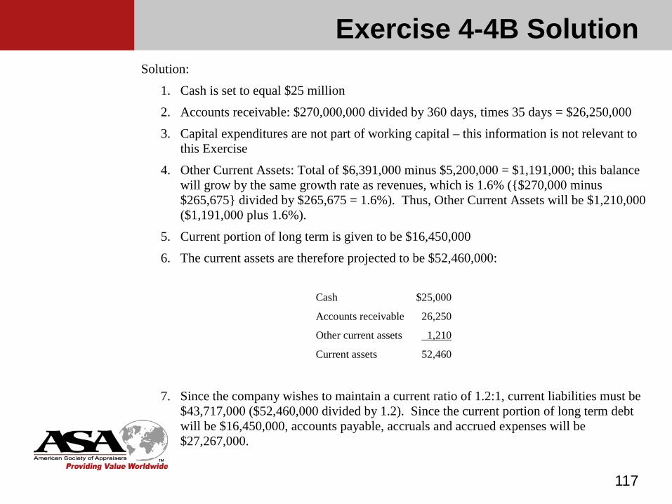
Solution:
1. Cash is set to equal $25 million
2. Accounts receivable: $270,000,000 divided by 360 days, times 35 days = $26,250,000
3. Capital expenditures are not part of working capital – this information is not relevant to this Exercise
4. Other Current Assets: Total of $6,391,000 minus $5,200,000 = $1,191,000; this balance will grow by the same growth rate as revenues, which is 1.6% ({$270,000 minus $265,675} divided by $265,675 = 1.6%). Thus, Other Current Assets will be $1,210,000 ($1,191,000 plus 1.6%).
5. Current portion of long term is given to be $16,450,000
6. The current assets are therefore projected to be $52,460,000:
Cash $25,000
Accounts receivable 26,250
Other current assets 1,210
Current assets 52,460
7. Since the company wishes to maintain a current ratio of 1.2:1, current liabilities must be $43,717,000 ($52,460,000 divided by 1.2). Since the current portion of long term debt will be $16,450,000, accounts payable, accruals and accrued expenses will be $27,267,000.
Developing the projection
Function of the projected revenue, expenses, and balance sheet components
Financial ratios for the projected period should be calculated and compared with the subject company’s historical results and with industry or peer group benchmarks
118
Developing the projection
Problems with percent of sale projections May overlook management objectives such as improved
margins, improved efficiencies, asset management May overlook changes in pricing strategies Assumes linear relationships
119
Management projections
Review assumptions Evaluate management’s historical ability to meet its
projections Investigate potential bias in/ulterior motives for the
projection For example, a projection prepared to raise capital may be overly
optimistic
Perform ratio and sensitivity analyses on the projection
120
If uncomfortable with the projection Attempt to reconcile with management Utilize a multi-scenario method Prepare independent projection(s) Adjust the discount rate (not recommended, except for
start ups, VC’s – addressed later) Resign from engagement (method of last resort)
121
Management projections
Exercise 4-5
122
ASSESSING FACTORS FOR PROJECTIONSPlease read Exhibit 4-2 at the end of this chapter, then do Exercise 4-4 also at the end of this chapter.
Review an analysis of the history, economic, and industry data provided. Your assignment is to identify the most relevant factors and trends that may have an impact on a projection or projections for Spring Hill Furniture. You may also state how these relevant factors should be discussed with the company’s management in order to have a better understanding as to its impact on the projection or projections. Finally, relate these factors back to the three primary valuation variables: benefit stream (profitability), risk and growth.

Exercise 4-5 SOLUTION
123
IN CLASS DISCUSSION

Exercise 4-6
124
REVIEWING MANAGEMENT PROJECTIONSReview the company’s historical financial statements provided in Exhibit 4-3 and management-prepared projection provided in Exhibit 4-4. Identify any inconsistencies that may be evident in light of the information received in Exercise 4-5. State how these inconsistencies should be discussed with the company’s management to convey a better understanding of the reasonableness of the projection provided.
You can use the page provided at the end of Exhibit 4-4 to document your findings.

Exercise 4-6 SOLUTION
125
IN CLASS DISCUSSION
Projections of Nonlinear Relationships (p 51)
Economies of scale Inventory—when a large inventory base needs to be built up for
start-up sales, but additional sales require far less inventory investment (Example: large retailer such as Home Depot)
Property, plant, and equipment—investment occurs within relevant ranges of sales (No new investment is needed until sales capacity is reached; then a major investment is required.)
Projecting nonlinear assets Management input is required. Projecting tools here are usually beyond the scope of the
valuation assignment.
126
Projecting Stub Periods If the valuation date is other than year end, say June 30 for a company
with a December 31 year end, and the appraiser is working with historical financials through June 30, special considerations must be made. The appraiser must consider whether the company experiences any seasonality
in its sales, so that a simple annualization of the interim numbers would produce an erroneous result. For example, if a company has sales through six months of $5 million, but experiences a higher percentage of its sales in the fall season, simply annualizing sales to $10 million will understate revenues.
Similarly, if there are different product mixes or pricing structures during the first half of the year as compared to the second half, the gross profit percentage may differ in each portion of the year.
The appraiser must also use caution in drawing conclusions from comparing the most recent June 30 balance sheet with a series of five or more years of year end balance sheets. A company may maintain higher or lower balances of receivables, inventory, lines of credit, etc, during the year than at the end of the year.
127

Projecting Stub Periods
Special considerations, continued: In addition, the company may not record a full year’s worth of certain
expenses evenly throughout the year; for example, insurance expense may be recorded when paid, or year end bonuses or employee benefit accruals may not be recorded at all until year end.
Lastly, for smaller companies, interim financial statements are typically prepared internally, and not by the company’s independent accountant. This may lead to different classifications of various balances, or mispostings, that the independent accountant has not yet corrected.
For all these reasons, extra care must be exercised when using interim financial data in your analysis
128

Common Errors
Unsupported assumptions Significant sales growth without commensurate
investment in working capital or fixed assets No analysis of fixed versus variable costs; all costs
assumed to be variable Working capital projection includes interest-bearing debt;
debt is then included in a separate debt principal projection
Other items of assets and liabilities omitted
129

Common Errors
Perpetuity growth higher than what can be sustained No re-examination of ratios to check the projection’s effect
on capital structure Use of historical averages Debt principal changes without consideration of its effect
on cost of debt or cost of equity.
130
Common Errors Cash flow projected into perpetuity includes impossible assumptions about
ongoing cap ex and depreciation, i.e. depreciation exceeding capital ex into perpetuity. Some analysts make the simplistic projection that capital ex will equal annual
depreciation, including in the final, stabilized period of the cash flow projection. On a long-term basis, this assumption would be valid only if the expected long
term growth is zero and the costs for the capital assets are expected to remain unchanged.
Most analysts agree that over the long term, annual capital ex will exceed the annual depreciation expense because:
Rising costs of capital assets: the depreciation expense in any given year is based on the cost of the capital asset base when those assets were acquired and will be replaced with higher-priced assets
Growth will require additional assets:the depreciation expense in any given year is based on the capital assets employed at the time. Growth will require that the company add assets to the capital asset base.
131

Common Errors
Depreciation and capital expenditures (cont’d) Daniel McConaughy and Lorena Bordi study
the long term capital expenditures exceeded depreciation across all industries, some more than others.
those that make the assumption in the single period model that capital expenditures equal depreciation will overstate value.
depending on the industry, profitability, and growth, the overstatement can be significant.
132

Common Errors
Depreciation and capital expenditures (cont’d) Brant Armentrout model
the author developed a model to reflect the expected long term ratio of depreciation to capital expenditures (expressed as a %) to be used as a “sanity check” for the analysts projections of those variables.
Armentrout suggests that long term capital expenditure needs are closely related to sales allowing the analyst to reasonably projection capital expenditures relative to the revenue projection.
133
Common Errors
Depreciation and capital expenditures (cont’d) Brant Armentrout model
The greater the long term growth, the lower the ratio of depreciation to capital expenditures (and vice versa).
The greater the average depreciable lives of the asset base the lower the ratio of depreciation to capital expenditures (and vice versa).
134

Common Errors
In the terminal year, cash flow from changes in debt usually should result in an increase in cash flow. If it is a use of cash (debt repayment exceeds new
borrowings) then, given enough time, all the debt will be repaid and, ultimately, the subject company will be lending money to the bank! If debt repayment equals new borrowings in the terminal
year, the implication is that the balance of debt will remain unchanged, which is unlikely for a company that is expected to grow into perpetuity.
135

Exercise 4-7-Projecting GDT’s Financials
In this exercise you will develop your own projections for General Delivery Trucking (GDT). See Chapter 11 for information to help you develop your projection assumptions.
136

Chapter 5
Capitalization of Benefits Method
137

Definitions and Formula (page 91)
Also known as the “Single Period Capitalization Method”
Capitalization—the conversion of a single period of economic benefits into value (BV Standards Glossary)
Capitalization factor—any multiple or divisor used to convert anticipated economic benefits of a single period into value (BV Standards Glossary)
138
Definitions and Formula
Capitalization rate—any divisor (usually expressed as a percentage) used to convert anticipated economic benefits of a single period into value (BV Standards Glossary)
Capitalization of benefits method is based on the formula for calculating the value of an anticipated economic benefit of a single period growing at a constant rate in perpetuity.
139
Definitions and Formula
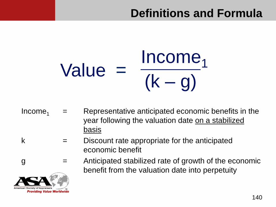
Income1 = Representative anticipated economic benefits in the year following the valuation date on a stabilized basis
k = Discount rate appropriate for the anticipated economic benefit
g = Anticipated stabilized rate of growth of the economic benefit from the valuation date into perpetuity
140
Income1(k – g)=Value
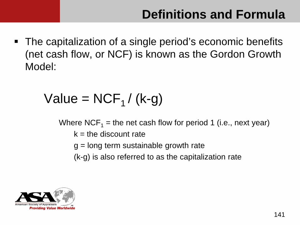
The capitalization of a single period’s economic benefits (net cash flow, or NCF) is known as the Gordon Growth Model:
Value = NCF1 / (k-g)
Where NCF1 = the net cash flow for period 1 (i.e., next year)k = the discount rateg = long term sustainable growth rate(k-g) is also referred to as the capitalization rate
141
Definitions and Formula
The Gordon Growth Model is used when the expected economic benefit for next year (period 1) is expected to grow at a stable long term rate (k-g) into perpetuity.
142
Definitions and Formula
Definitions and Formula
The economic benefits figure in the capitalization formula is next year’s anticipated economic benefits.
This is a function of the mathematical derivation of the growing perpetuity formula.
A capitalization of benefits method is identical to a discounted future benefits method assuming a constant growth rate in future income.
143
Definitions and Formula
Capitalization of Benefits Method Example The company’s equity net cash flow has grown during the
most recent five fiscal years at a compound annual growth rate of about 5%. Normalized equity net cash flow for the next fiscal year is
projected at $600,000. A discount rate for the company is 22%. The anticipated long-term growth rate in equity net cash
flow is 4%.
144
Definitions and Formula
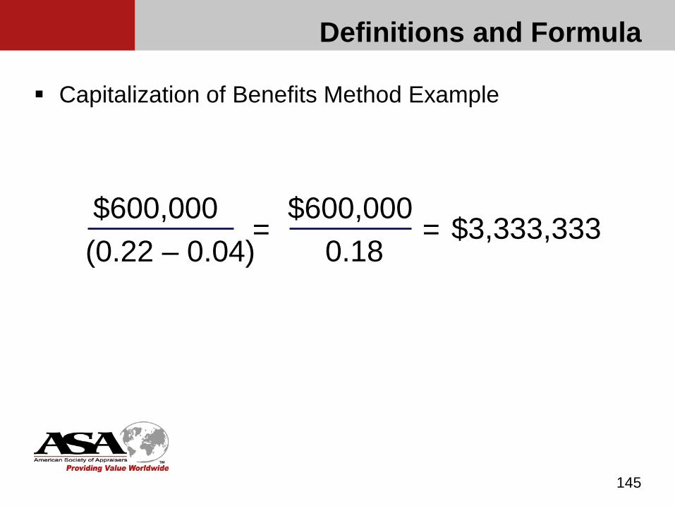
Capitalization of Benefits Method Example
145
$600,000(0.22 – 0.04)
= $3,333,333$600,000
0.18=
Model Components
The Economic Benefits to be Capitalized Economic benefits from stabilized operations which
represents future anticipated economic benefits The anticipated economic benefit that best represents
future expectations varies with business trends. Most recent results For a declining business (negative growth), this approach is
generally inappropriate. Simple average of results over an entire business cycle
146

Model Components
The Capitalization Rate Capitalization rates can be developed on an equity basis
or an invested capital basis. Adjustments necessary to develop capitalization rates for
other levels of economic benefits are discussed at the end of this chapter.
147
Model Components
The Capitalization Rate Other sources of capitalization rates: The public stock markets—The analyst must be
satisfied that the companies selected for comparative purposes are sufficiently similar to the subject to provide meaningful data. Transaction data
148
Model Components
The Capitalization Rate Discount Rates External factors such as national and local economic
conditions and outlook, national and local industry conditions and outlook, cost and availability of capital, competition, etc. Internal factors include financial condition of the
business (leverage, available cash, current ratio, etc.), quality of earnings (historic levels, margins, etc), quality of management, customer base, etc.
149
Model Components
The Capitalization Rate Long-Term Growth The long-term rate of growth should be one that can
be sustained into perpetuity. The growth rate should take into consideration the
business’s current position in its life cycle. Over a prolonged period of time it is difficult to sustain
growth that exceeds the rate of inflation plus the real rate of growth in terms of the population (GDP growth).
150

Use in Market Approach (page 94)
A multiple is the inverse of a capitalization rate
Cap Rate = 1 / MultipleMultiple = 1 / Cap Rate
If the Price/Equity Cash Flow multiple = 15 and the equity cash flow estimated long- term growth rate is 3%, what is the implied equity discount rate?
Cap Rate = 1 / Multiple = 1 / 15 = 6.67% Cap Rate = Discount Rate – Growth Discount rate = Cap Rate + Growth = 6.67% + 3.00% = 9.67%
151

Use in Market Approach
Some would argue, however, that investors in the public securities have a shorter holding period expectation (less than two years) than investors in private securities. Longer holding period means greater risk.
Therefore, their “long-term” growth consideration is three to five years, not perpetuity. This often results in greater growth expectations by public investors than their private counterparts.
152
Use in Market Approach
Distinctions in the application of the method in the income and market approaches. In the market approach, growth is embedded in the market multiple
(the inverse of the capitalization rate) In the income approach, growth must be quantified and is reflected in
the benefit stream and the capitalization rate.
153
Cap Rate Sensitivity
Value conclusions are very sensitive to the selected capitalization rate.
For example, for a company with anticipated future net equity cash flow of $500,000, increasing the 18% capitalization rate by two percentage points to 20% reduces the value of the subject company from $2.778 million to $2.500 million or by about 10%.
154
Exercise 5-1
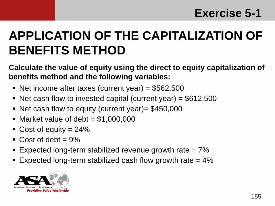
155
APPLICATION OF THE CAPITALIZATION OF BENEFITS METHODCalculate the value of equity using the direct to equity capitalization of benefits method and the following variables: Net income after taxes (current year) = $562,500 Net cash flow to invested capital (current year) = $612,500 Net cash flow to equity (current year)= $450,000 Market value of debt = $1,000,000 Cost of equity = 24% Cost of debt = 9% Expected long-term stabilized revenue growth rate = 7% Expected long-term stabilized cash flow growth rate = 4%
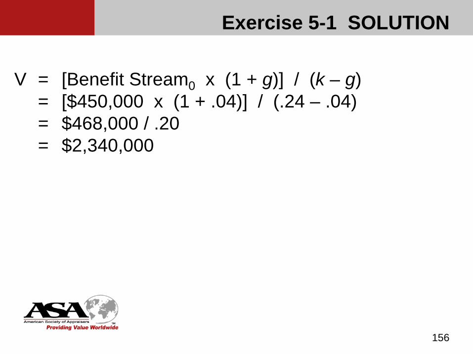
Exercise 5-1 SOLUTION
156
V = [Benefit Stream0 x (1 + g)] / (k – g)= [$450,000 x (1 + .04)] / (.24 – .04)= $468,000 / .20= $2,340,000

Capitalization rates differ for varying levels of anticipated economic benefits. (The higher up the P&L the level of anticipated economic benefits is, the higher the capitalization rate.)
157
Cap Rates for Other Income Measures

Cap Rates for Other Income Measures
Converting an equity net cash flow capitalization rate to a net income capitalization rate: The first step is to identify the normalized relationship
between net income and equity net cash flow. Calculate the annual historical ratios of net income to equity net
cash flow. Adjust for any anticipated changes in the future. Depending on the facts and circumstances of the engagement,
an analysis of similar ratios for publicly traded companies over time may provide support for the normalized relationship.
158

Converting an equity net cash flow capitalization rate to a net income capitalization rate (cont’d): With the important assumption that the ratio between net
income and equity net cash flow is constant in the future, the conversion formula is:
CRnet income = NI/NCF CRnet cash flowCR = Capitalization rateNI = Net incomeNCF = Equity net cash flow
159
Cap Rates for Other Income Measures
Converting an equity net cash flow capitalization rate to a net income capitalization rate (cont’d): If normalized net income is expected to be 125% of
normalized equity net cash flow, a 20.0% net cash flow capitalization rate translates into a 25% net income capitalization rate:
1.25 x 20.0% = 25%
160
Cap Rates for Other Income Measures
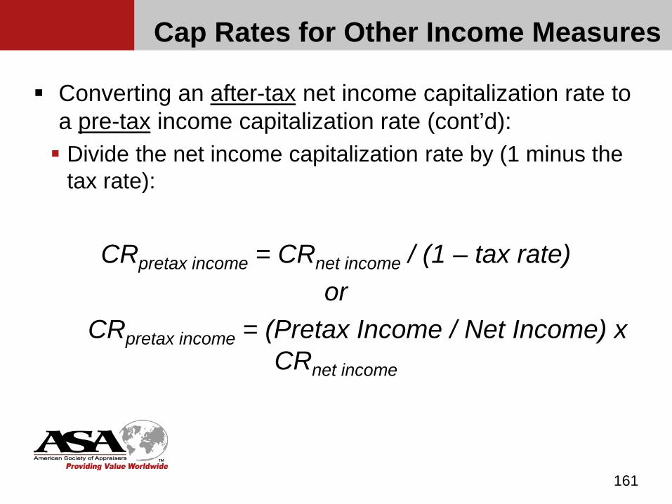
Converting an after-tax net income capitalization rate to a pre-tax income capitalization rate (cont’d): Divide the net income capitalization rate by (1 minus the
tax rate):
CRpretax income = CRnet income / (1 – tax rate)or
CRpretax income = (Pretax Income / Net Income) x CRnet income
161
Cap Rates for Other Income Measures
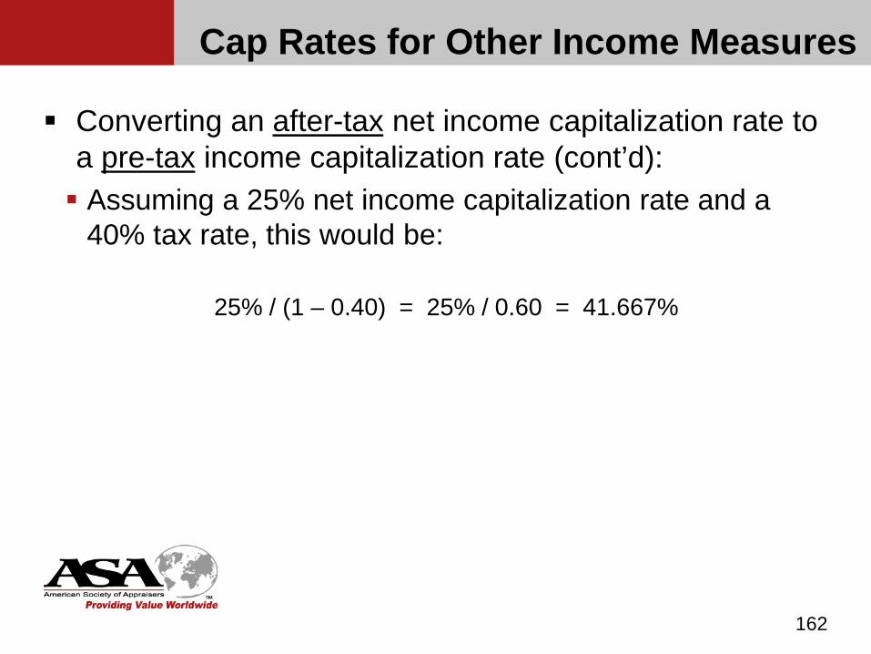
Converting an after-tax net income capitalization rate to a pre-tax income capitalization rate (cont’d): Assuming a 25% net income capitalization rate and a
40% tax rate, this would be:
25% / (1 – 0.40) = 25% / 0.60 = 41.667%
162
Cap Rates for Other Income Measures

Capitalization rates can be adjusted based on the relationships between the measures of income: Pre-tax earnings capitalization rate = After-tax earnings
capitalization rate x (pre-tax earnings / after-tax earnings) Net income capitalization rate = Cash flow capitalization
rate x (net income / cash flow) However, the same is not true for converting discount
rates due to growth.
163
Cap Rates for Other Income Measures
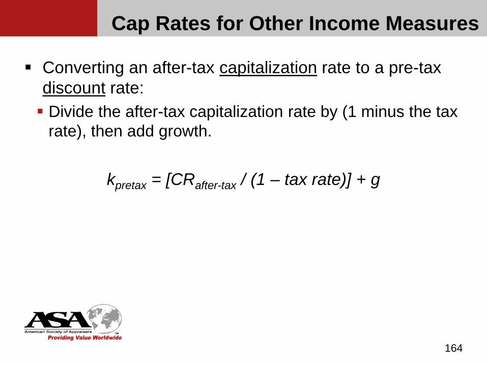
Converting an after-tax capitalization rate to a pre-tax discount rate: Divide the after-tax capitalization rate by (1 minus the tax
rate), then add growth.
kpretax = [CRafter-tax / (1 – tax rate)] + g
164
Cap Rates for Other Income Measures
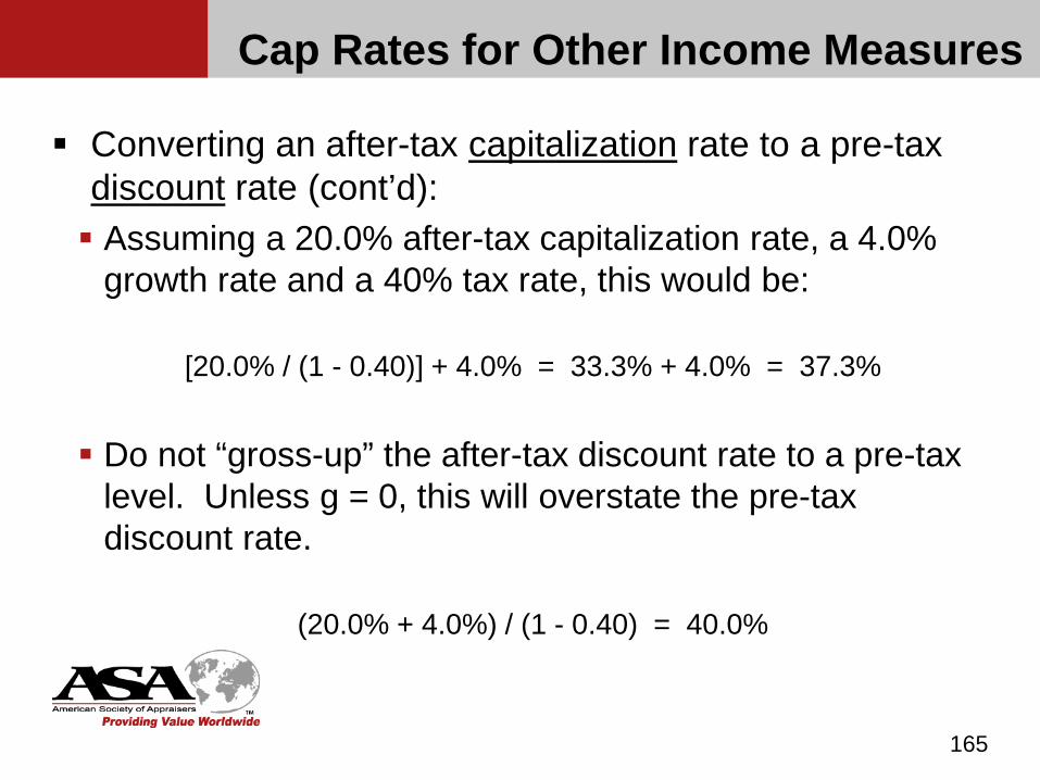
Converting an after-tax capitalization rate to a pre-tax discount rate (cont’d): Assuming a 20.0% after-tax capitalization rate, a 4.0%
growth rate and a 40% tax rate, this would be:
[20.0% / (1 - 0.40)] + 4.0% = 33.3% + 4.0% = 37.3%
Do not “gross-up” the after-tax discount rate to a pre-tax level. Unless g = 0, this will overstate the pre-tax discount rate.
(20.0% + 4.0%) / (1 - 0.40) = 40.0%
165
Cap Rates for Other Income Measures
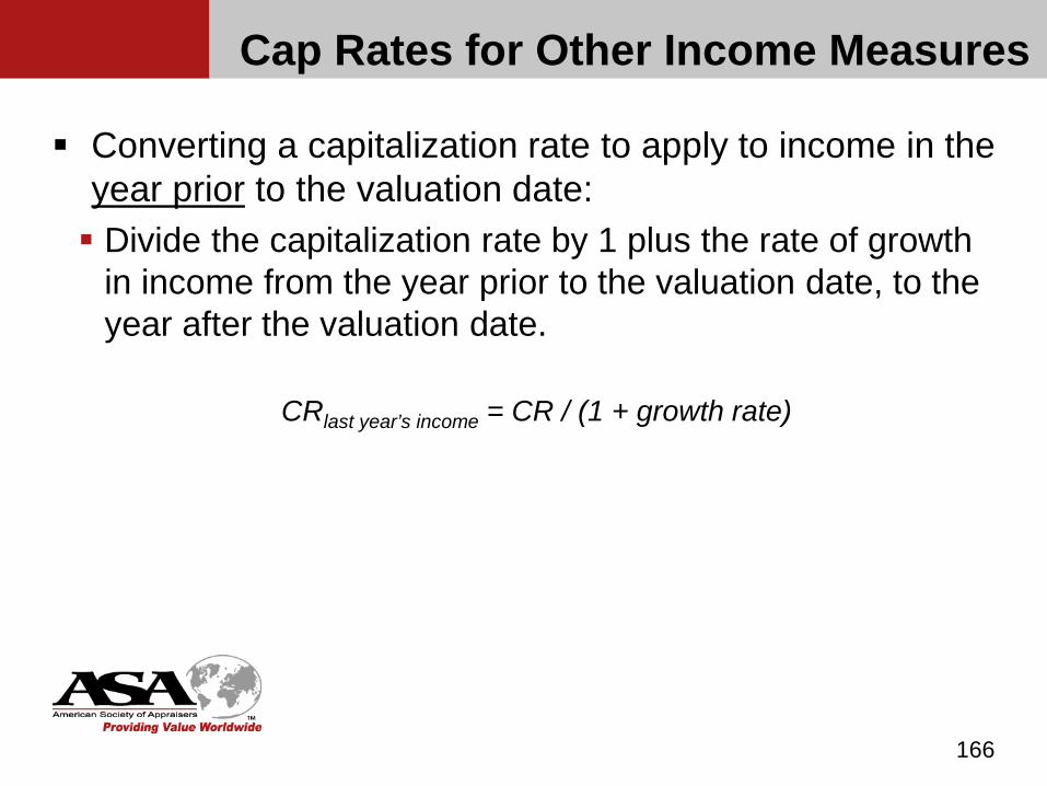
Converting a capitalization rate to apply to income in the year prior to the valuation date: Divide the capitalization rate by 1 plus the rate of growth
in income from the year prior to the valuation date, to the year after the valuation date.
CRlast year’s income = CR / (1 + growth rate)
166
Cap Rates for Other Income Measures
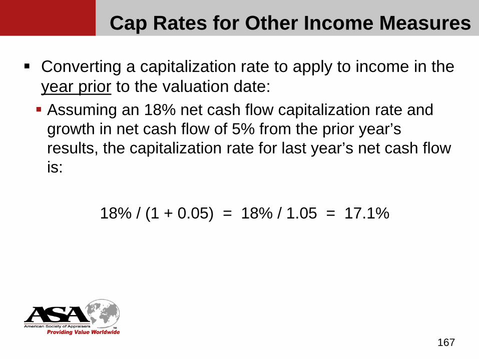
Converting a capitalization rate to apply to income in the year prior to the valuation date: Assuming an 18% net cash flow capitalization rate and
growth in net cash flow of 5% from the prior year’s results, the capitalization rate for last year’s net cash flow is:
18% / (1 + 0.05) = 18% / 1.05 = 17.1%
167
Cap Rates for Other Income Measures
Exercise 5-2
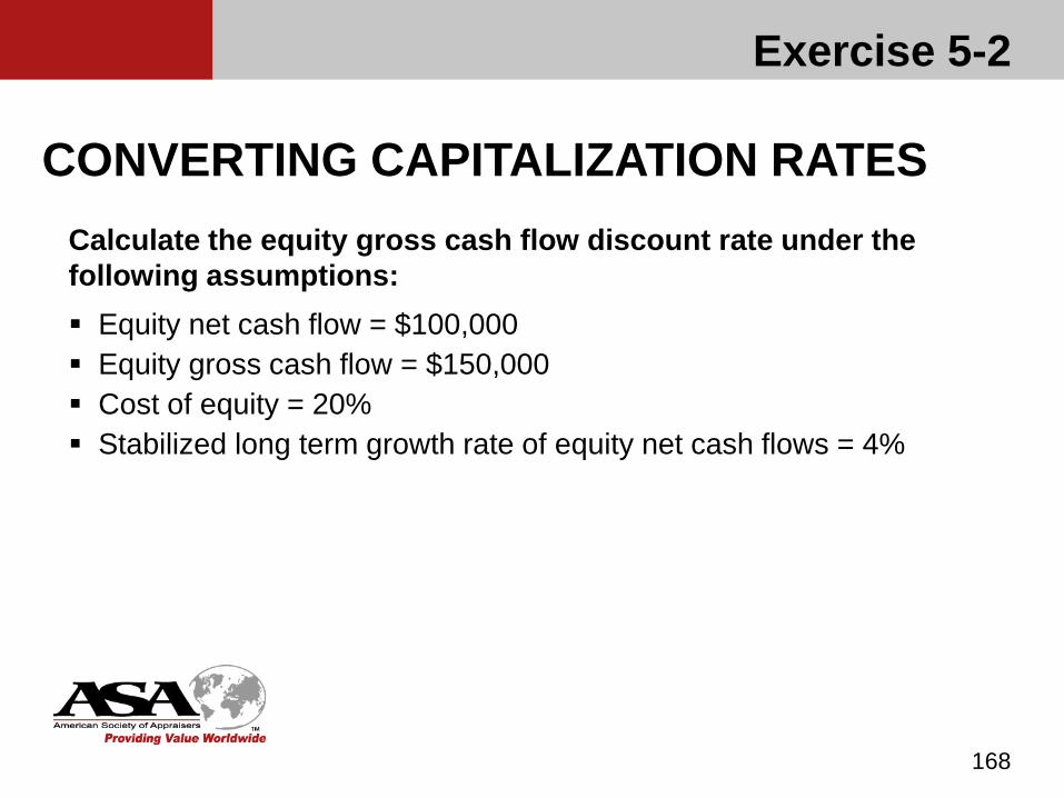
168
CONVERTING CAPITALIZATION RATESCalculate the equity gross cash flow discount rate under the following assumptions: Equity net cash flow = $100,000 Equity gross cash flow = $150,000 Cost of equity = 20% Stabilized long term growth rate of equity net cash flows = 4%
Exercise 5-2 SOLUTION
169
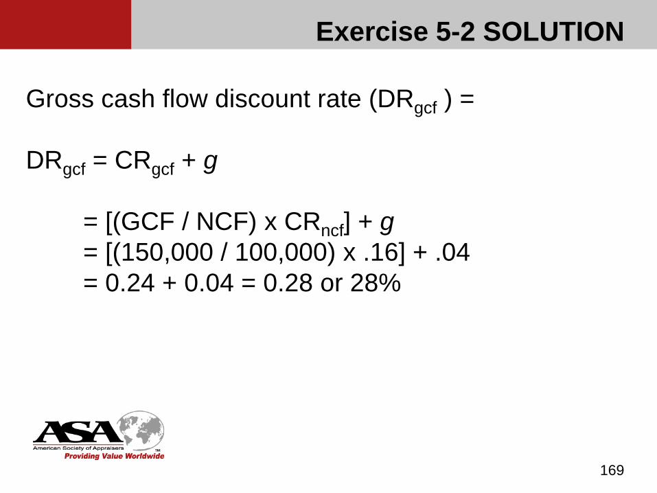
Gross cash flow discount rate (DRgcf ) =
DRgcf = CRgcf + g
= [(GCF / NCF) x CRncf] + g= [(150,000 / 100,000) x .16] + .04= 0.24 + 0.04 = 0.28 or 28%

Because the exercise asks for the equity gross cash flow discount rate, not capitalization rate, a growth rate must be added to the equity cash flow capitalization rate.
It is important to note that only in a stable state will the expected long-term growth rate be the same for different levels of benefit streams.
170
Exercise 5-2 SOLUTION
Chapter 6
Discounted Future Benefits Method
171
Definitions and Formula (page 102)
Also known as the “Multi Period Discounting Method” Allows for greater flexibility and precision in reflecting
known variations in the future anticipated economic benefits of a business.
172
Definitions and Formula
The discounted future benefits method involves the following steps: Determine what benefit stream measure to use. Projection the benefit stream for a period of years (the discrete
projection period). Discount each year’s benefit stream to present value at the
appropriate discount rate. Sum the present values of the explicit projection benefit streams.
173
Definitions and Formula
The discounted future benefits method involves the following steps (cont’d): Determine the value of the business at the end of the discrete
projection period, which is variously known as the terminal value, continuing value, or residual value of the business.
Add the present value of the terminal value to the present value of the discrete projection period benefit streams.
174
Definitions and Formula
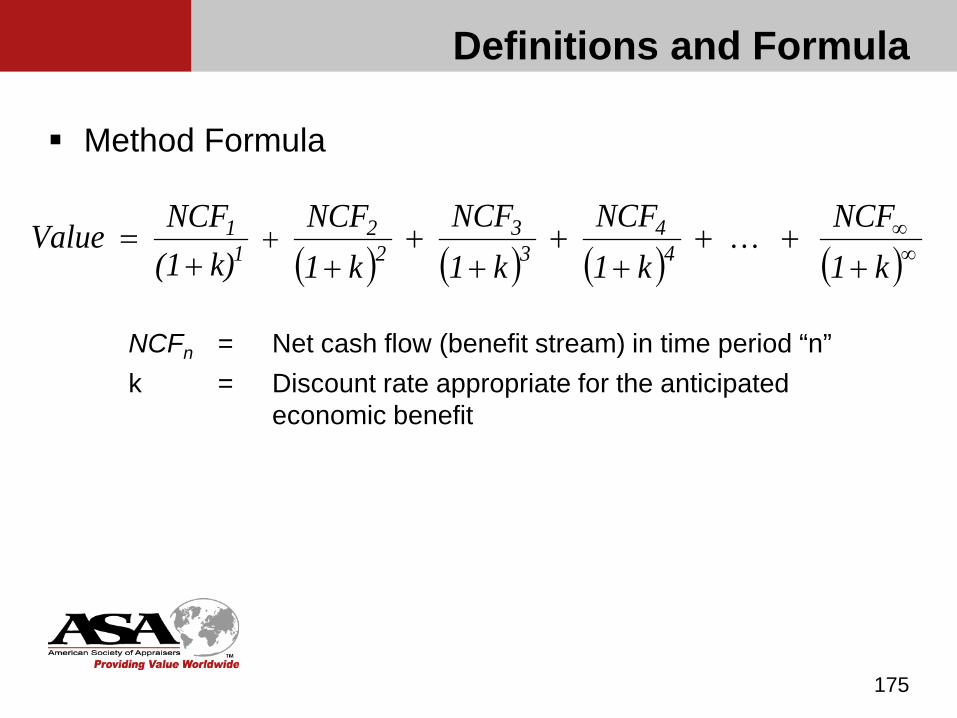
Method Formula
175
( ) ( ) ( ) ( )∞∞
+++
++
++
++= +
k1NCF
k1NCF
k1NCF
k1NCF
k)(1NCF Value 4
43
32
21
1
NCFn = Net cash flow (benefit stream) in time period “n”k = Discount rate appropriate for the anticipated
economic benefit

Definitions and Formula
This equation can also be expressed as:
176
NCFn = Net cash flow (benefit stream) in time period “n”k = Discount rate appropriate for the anticipated economic
benefitn = Time period
∑∞=
= +=
n
nn
n
kNCFValue
1 1 )(
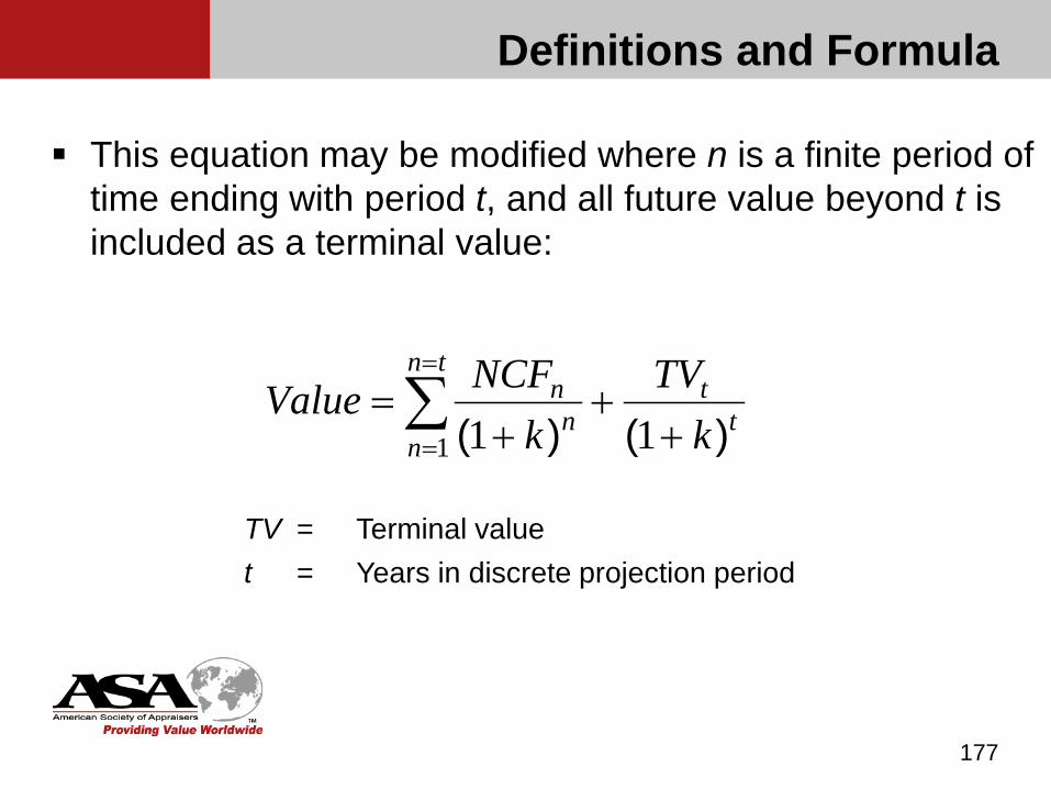
Definitions and Formula
This equation may be modified where n is a finite period of time ending with period t, and all future value beyond t is included as a terminal value:
177
TV = Terminal valuet = Years in discrete projection period
tt
tn
nn
n
kTV
kNCFValue
)()( ++
+= ∑
=
= 111
Key Elements in Method
The length of the discrete projection period Explicit projections should be made for a period long
enough to get beyond circumstances that are unusual or atypical (stabilized conditions – see examples in outline). A common practice is to use a discrete projection period
of five years, but there is no inherent economic logic to five years as opposed to four, six, or some other number of years.
178

Key Elements in Method
The length of the discrete projection period The choice of a projection horizon should depend on the
specific circumstances of the subject company and should be long enough to achieve stabilized earnings and cash flow.
179
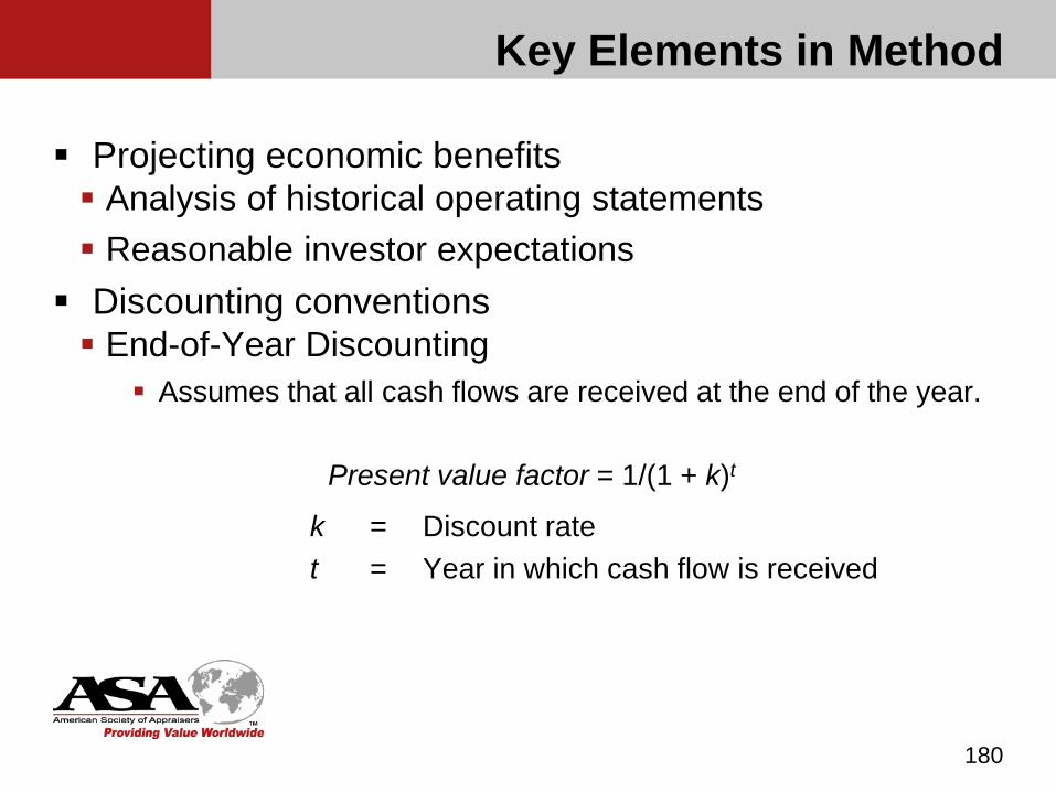
Key Elements in Method
Projecting economic benefits Analysis of historical operating statements Reasonable investor expectations Discounting conventions End-of-Year Discounting
Assumes that all cash flows are received at the end of the year.
Present value factor = 1/(1 + k)t
k = Discount ratet = Year in which cash flow is received
180

Key Elements in Method
Discounting Conventions (cont’d) Mid-Year Discounting
When cash flows are received relatively evenly throughout the year, an alternative discounting methodology is appropriate.
The present value factor for the mid-year discounting convention is calculated as follows:
Present value factor = 1/(1 + k)(t – 0.5)
181
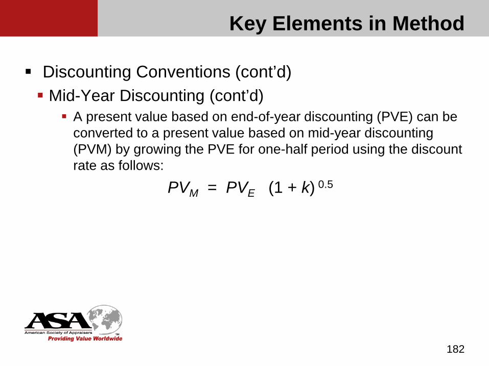
Key Elements in Method
Discounting Conventions (cont’d) Mid-Year Discounting (cont’d)
A present value based on end-of-year discounting (PVE) can be converted to a present value based on mid-year discounting (PVM) by growing the PVE for one-half period using the discount rate as follows:
PVM = PVE (1 + k) 0.5
182
Key Elements in Method
Discounting Conventions (cont'd) Seasonal retail businesses, dependent on holiday
sales—end-of-year convention Non-seasonal business—typically mid-year convention Use of a discounting convention should be a decision
based upon the facts and circumstances of the engagement. The discounting convention can be something other than end-of-year or mid-year if warranted by the facts and circumstances.
183

Exercise 6-1
184
MULTIPLE PERIOD DISCOUNTINGCalculate the present value of the following net equity cash flows using both end-of-year and mid-year discounting conventions using the following data. Do not attempt to calculate the terminal value at this time. That will be addressed in a later exercise. • Appraisal date = December 31, 20X0• Long-term growth rate = 4%• Discount rate = 20%• Projected net cash flows to equity:
20X1 = $525,00020X2 = $572,00020X3 = $618,00020X4 = $661,00020X5 = $687,000
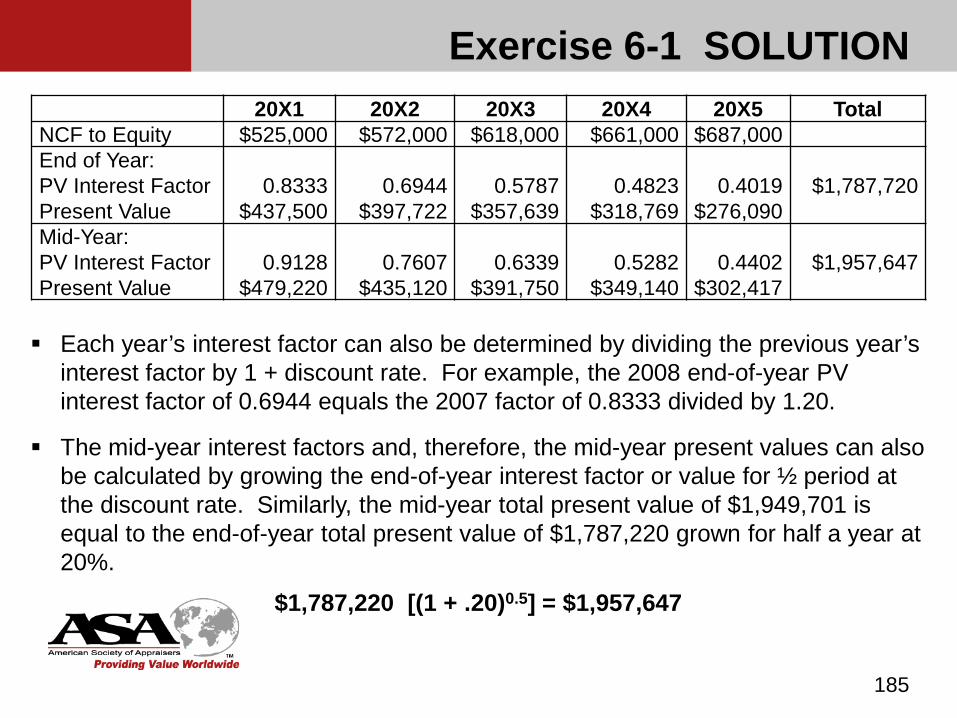
Exercise 6-1 SOLUTION
185
Each year’s interest factor can also be determined by dividing the previous year’s interest factor by 1 + discount rate. For example, the 2008 end-of-year PV interest factor of 0.6944 equals the 2007 factor of 0.8333 divided by 1.20.
The mid-year interest factors and, therefore, the mid-year present values can also be calculated by growing the end-of-year interest factor or value for ½ period at the discount rate. Similarly, the mid-year total present value of $1,949,701 is equal to the end-of-year total present value of $1,787,220 grown for half a year at 20%.
$1,787,220 [(1 + .20)0.5] = $1,957,647
20X1 20X2 20X3 20X4 20X5 TotalNCF to Equity $525,000 $572,000 $618,000 $661,000 $687,000End of Year:PV Interest FactorPresent Value
0.8333$437,500
0.6944$397,722
0.5787$357,639
0.4823$318,769
0.4019$276,090
$1,787,720
Mid-Year:PV Interest FactorPresent Value
0.9128$479,220
0.7607$435,120
0.6339$391,750
0.5282$349,140
0.4402$302,417
$1,957,647
Key Elements in Method
Calculating terminal value The terminal value is defined as “the value [of the
business] as of the end of the discrete projection period in a discounted future benefits model” (BV Standards Glossary).
186
Key Elements in Method
Calculating terminal value (cont’d) Some alternatives to calculating the terminal value
include: Liquidation value Capitalization of the stabilized benefit stream as of the
end of the discrete projection period Application of a current (or forward-looking) market
multiple
187

Calculating terminal value (cont’d) The terminal value formula when using the Gordon
Growth Model is as follows:
Net cash flow in the last year of the explicit projection should grow at the long-term growth rate.
If there is a different growth rate in the last year of the projection than is used for the long-term growth assumption, the required change in working capital and fixed assets will be misstated in the terminal value factor.
188
(1 )Terminal Value
NCF gtk g× +
= −
Key Elements in Method
The Gordon Growth Model (used in the Single Period Capitalization Method) is also used in computing the Terminal Value because the same criteria are present:
The expected economic benefit for next year (period T) is expected to grow at a stable long term rate (k-g) into perpetuity.
Period T (the terminal year) replaces period 1 that was used in the Single Period Capitalization Method.
189
Key Elements in Method
Key Elements in Method
Calculating terminal value (cont’d) Present value of the terminal value Observations on Terminal Value
Forever is a long, long time. Typically, modest growth (3% to 5%) is assumed in the terminal value factor.
The growth rate may reflect little more than inflation, population growth, and minor productivity or demand changes.
190
Key Elements in Method
Calculating terminal value (cont’d) Observations on Terminal Value
An exit or liquidation value may be more appropriate in some cases. The depreciation/capital expenditure relationship must make sense. The change in debt assumptions must make sense In most applications of the discounted future benefits method, the
terminal value can represent a substantial portion of the overall value of the business. Therefore, particular care must be exercised in its derivation.
191
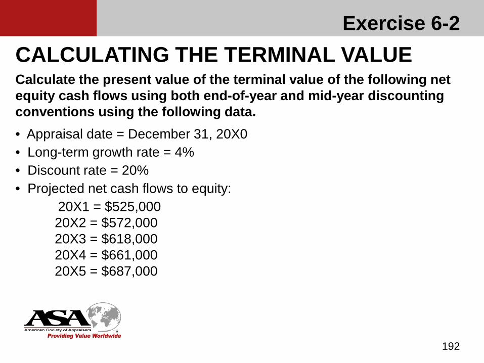
Exercise 6-2
192
CALCULATING THE TERMINAL VALUECalculate the present value of the terminal value of the following net equity cash flows using both end-of-year and mid-year discounting conventions using the following data. • Appraisal date = December 31, 20X0• Long-term growth rate = 4%• Discount rate = 20%• Projected net cash flows to equity:
20X1 = $525,00020X2 = $572,00020X3 = $618,00020X4 = $661,00020X5 = $687,000
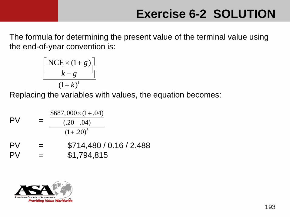
Exercise 6-2 SOLUTION
193
The formula for determining the present value of the terminal value using the end-of-year convention is:
Replacing the variables with values, the equation becomes:
PV =
PV = $714,480 / 0.16 / 2.488PV = $1,794,815
5
$687,000 (1 .04)(.20 .04)(1 .20)
× +−
+
NCF (1 )
(1 )
t
t
gk g
k
× + −
+
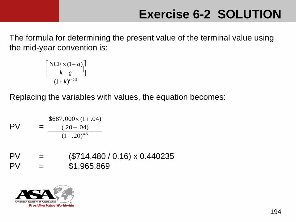
Exercise 6-2 SOLUTION
194
The formula for determining the present value of the terminal value using the mid-year convention is:
Replacing the variables with values, the equation becomes:
PV =
PV = ($714,480 / 0.16) x 0.440235 PV = $1,965,869
0.5
NCF (1 )
(1 )
t
t
gk g
k −
× + −
+
4.5
$687,000 (1 .04)(.20 .04)(1 .20)
× +−
+
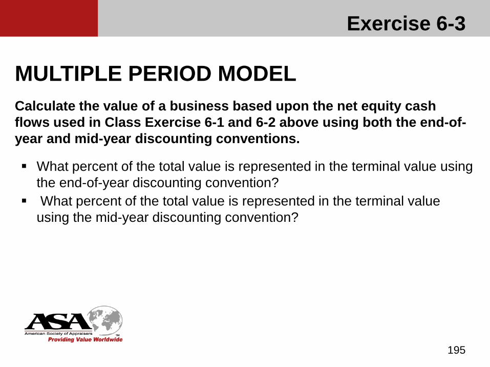
Exercise 6-3
195
MULTIPLE PERIOD MODELCalculate the value of a business based upon the net equity cash flows used in Class Exercise 6-1 and 6-2 above using both the end-of-year and mid-year discounting conventions.
What percent of the total value is represented in the terminal value using the end-of-year discounting convention?
What percent of the total value is represented in the terminal value using the mid-year discounting convention?
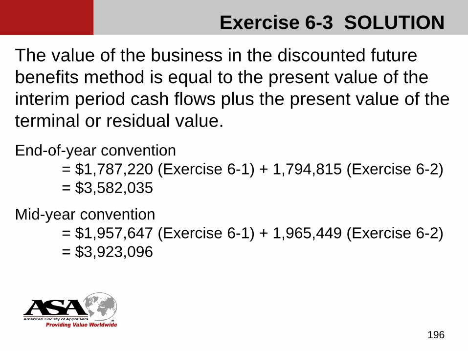
Exercise 6-3 SOLUTION
196
The value of the business in the discounted future benefits method is equal to the present value of the interim period cash flows plus the present value of the terminal or residual value.End-of-year convention
= $1,787,220 (Exercise 6-1) + 1,794,815 (Exercise 6-2)= $3,582,035
Mid-year convention= $1,957,647 (Exercise 6-1) + 1,965,449 (Exercise 6-2) = $3,923,096

Exercise 6-4
197
SENSITIVITY ANALYSISCalculate the value of a business based upon the net equity cash flows used in Class Exercise 6-1 and 6-2 above but change the discount rate to 18%. Use the end-of-year discounting convention. What was the percentage change in the discount rate? What was the resulting percentage change in the calculated value?
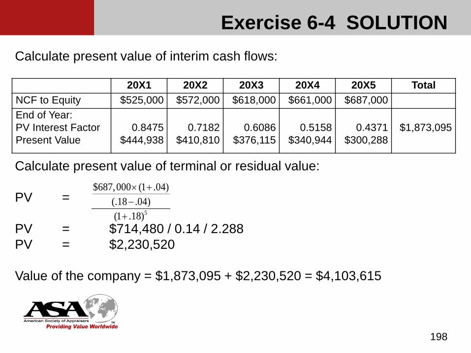
Exercise 6-4 SOLUTION
198
Calculate present value of interim cash flows:
Calculate present value of terminal or residual value:
PV =
PV = $714,480 / 0.14 / 2.288PV = $2,230,520
Value of the company = $1,873,095 + $2,230,520 = $4,103,615
20X1 20X2 20X3 20X4 20X5 TotalNCF to Equity $525,000 $572,000 $618,000 $661,000 $687,000End of Year:PV Interest FactorPresent Value
0.8475$444,938
0.7182$410,810
0.6086$376,115
0.5158$340,944
0.4371$300,288
$1,873,095
5
$687,000 (1 .04)(.18 .04)(1 .18)
× +−
+
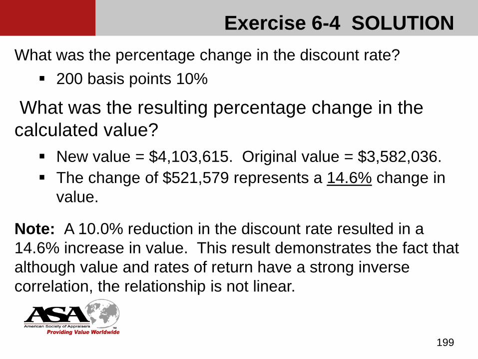
Exercise 6-4 SOLUTION
199
What was the percentage change in the discount rate? 200 basis points 10%
What was the resulting percentage change in the calculated value? New value = $4,103,615. Original value = $3,582,036. The change of $521,579 represents a 14.6% change in
value.
Note: A 10.0% reduction in the discount rate resulted in a 14.6% increase in value. This result demonstrates the fact that although value and rates of return have a strong inverse correlation, the relationship is not linear.
Chapter 7
Introduction to Discount Rates
200
Definitions and Terminology (page 113)
Discount rate—a rate of return used to convert a monetary sum, payable or receivable in the future, into present value (BVS Definitions)
The discount rate is equal to the “cost of capital”—the expected rate of return that the market requires in order to attract funds to a particular investment (BVS Definitions).
201

Definitions and Terminology
The discount rate is based on the principle of determining the appropriate rate of return given the risk of the subject investment. The rate should be higher than for investments of lower risk levels, and lower for investments of higher risk levels, other things being equal.
Considerations for the discount rate are: A risk-free rate Premium for risk, or risk premium
“Risk” can be related to size, industry, and factors specific to the subject company
202
Definitions and Terminology
Different discount rates for various levels of capital Interest-bearing debt: prevailing interest rates plus costs
of debt Common equity: cost of or required rate of return on
common equity Preferred equity: cost of or required rate of return on
preferred equity
203
Definitions and Terminology
Different discount rates for various levels of capital (cont’d) Total equity: weighted costs of common equity and
preferred equity Invested capital: weighted costs common equity,
preferred equity, and interest-bearing permanent debt
204
Definitions and Terminology
Other terms often used to describe a discount rate: Cost of capital Rate of return Required rate of return Cost of equity Weighted average cost of capital Alternative cost of capital Hurdle rate
205
Risk-Return-Discount Rate
In the context of the discount rate, risk is defined as the degree of uncertainty as to the realization of the future benefits stream.
There is a positive relationship between risk and return. There is a negative relationship between the discount
rate and value.
206
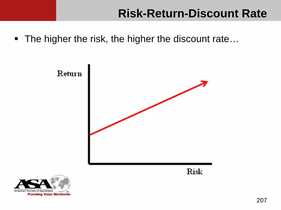
Risk-Return-Discount Rate
The higher the risk, the higher the discount rate…
207
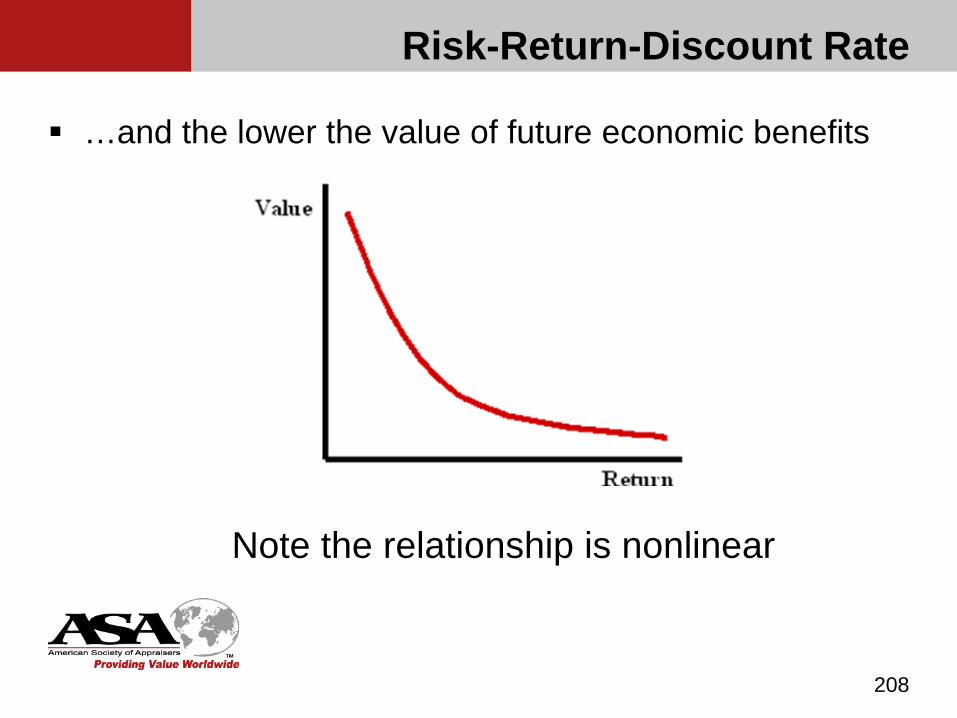
Risk-Return-Discount Rate
…and the lower the value of future economic benefits
Note the relationship is nonlinear
208

Risk-Return-Discount Rate (page 115)
Risk is associated with volatility, which can be measured as the probability distribution of potential returns on an investment (σ is the symbol for standard deviation).
The utility company is less risky and investors would demand a lower required of return for an investment. The tighter the probability distribution of returns on an investment given varying economic conditions, the lower the risk the investment will have.
209
- 2σ - 1σ Average + 1σ + 2σUtility Company 10% 11% 12% 13% 14%Car Dealer -24% -6% 12% 30% 48%
Types of Risk
Systematic (un-diversifiable) risk—the risk that is common to all risky securities and cannot be eliminated through diversification (BVS Definitions) Systematic risk is the uncertainty of future returns due to the
sensitivity of the return on the subject investment to movements in the return for the investment market as a whole.
210
Types of Risk
Systematic (un-diversifiable) risk (cont’d) Systematic risk includes the risks of systematic negative
events that affect all or most firms, such as war, recessions, interest rate cycles, etc. Other terms used to describe systematic risk:
Un-diversifiable risk Market risk
211
Types of Risk
Unsystematic (diversifiable) risk—the risk specific to an individual security that can be avoided through diversification (BVS Definitions) Unsystematic risk is the risk of random negative events
particular to a subject company such as labor strikes, failed product launches, lawsuits, departures of key personnel, etc.
212
Types of Risk
Unsystematic (diversifiable) risk (cont’d) Unsystematic risk may include industry risk depending on
the method used to determine the discount rate. Other terms used to describe unsystematic risk:
213
Unique risk Diversifiable risk Specific risk Investment-specific risk
Idiosyncratic risk Residual risk Company-specific risk
Characteristics of the Discount Rate
Determinants of the discount rate Market determined Forward-looking Varies with time, even for the same investment Incorporates inflationary expectation Based on returns available for alternative investments,
including returns on the broad equity market Must be adjusted for risk specific to the asset or right
being appraised
214
Characteristics of the Discount Rate
Determinants of the discount rate (cont’d) Depends on the nature of the future economic benefits Pre-tax or after tax Cash flow or income Equity or invested capital
215

Characteristics of the Discount Rate
Factors Affecting Discount Rate Selection External factors (those over which the managers of the
business have no control; see outline) Internal factors (those over which the managers of the
business have control; see outline)
216
Discount Rates
Cost of equity (ke) – Equity discount rate Weighted average cost of capital (WACC) –
Invested capital discount rate
217

Chapter 8
Developing the Equity Discount Rate
218
Methods (page 118) Build up method SBBI (now referred to as the Center for Research in
Security Prices, CRSP)
Duff & Phelps
Adjusted or Modified CAPM
219
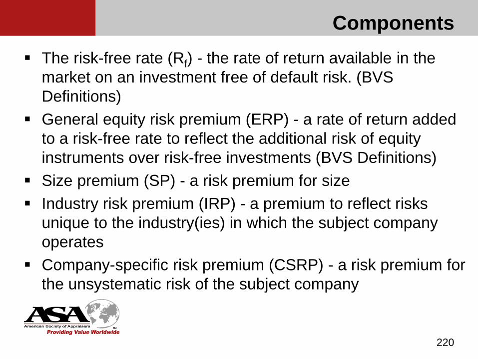
Components The risk-free rate (Rf) - the rate of return available in the
market on an investment free of default risk. (BVS Definitions)
General equity risk premium (ERP) - a rate of return added to a risk-free rate to reflect the additional risk of equity instruments over risk-free investments (BVS Definitions)
Size premium (SP) - a risk premium for size Industry risk premium (IRP) - a premium to reflect risks
unique to the industry(ies) in which the subject company operates
Company-specific risk premium (CSRP) - a risk premium for the unsystematic risk of the subject company
220
Overview: Build-up Method
Based on the principle that the discount rate is based on a number of identifiable risk factors that when added together result in the required rate of return for an equity investment in the company.
221
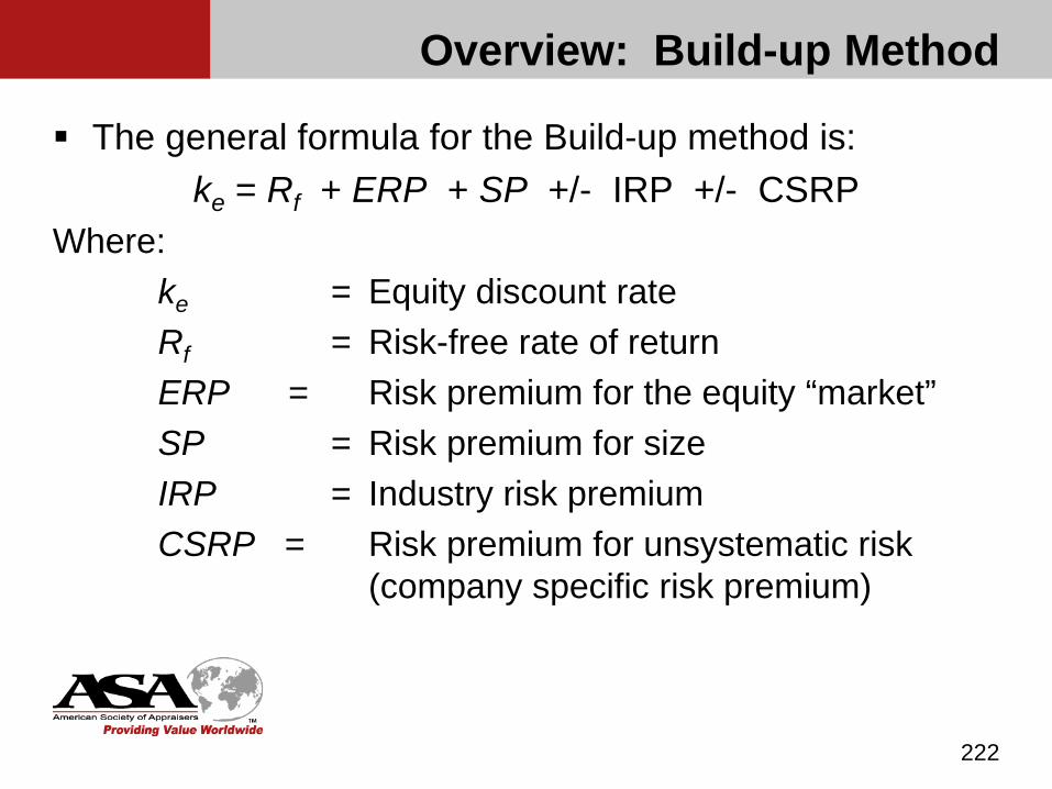
Overview: Build-up Method
The general formula for the Build-up method is:ke = Rf + ERP + SP +/- IRP +/- CSRP
Where:ke = Equity discount rateRf = Risk-free rate of returnERP = Risk premium for the equity “market” SP = Risk premium for sizeIRP = Industry risk premiumCSRP = Risk premium for unsystematic risk
(company specific risk premium)
222
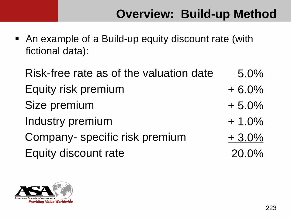
Overview: Build-up Method
An example of a Build-up equity discount rate (with fictional data):
223
Risk-free rate as of the valuation dateEquity risk premiumSize premiumIndustry premiumCompany- specific risk premiumEquity discount rate
5.0%+ 6.0%+ 5.0%+ 1.0%+ 3.0%20.0%
Risk-Free Rate of Return
Treasury securities There is agreement that Treasury securities are relatively
safe securities because their income payments and redemption dates are specified in advance, and they are virtually free of default risk. Differences in maturity introduce different risks
224
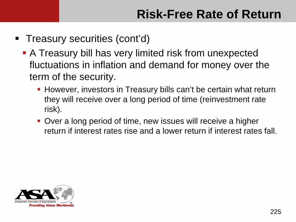
Risk-Free Rate of Return
Treasury securities (cont’d) A Treasury bill has very limited risk from unexpected
fluctuations in inflation and demand for money over the term of the security. However, investors in Treasury bills can’t be certain what return
they will receive over a long period of time (reinvestment rate risk).
Over a long period of time, new issues will receive a higher return if interest rates rise and a lower return if interest rates fall.
225

Risk-Free Rate of Return
Treasury securities (cont’d) Longer-term Treasury notes and bonds generally offer
higher returns than Treasury bills. Include an “investment horizon risk premium,” which
compensates investors for being locked in and unable to react to changing market conditions.
Accordingly, there is some debate about whether it is more accurate to use short-term Treasury bills or long-term Treasury bonds to represent the risk-free rate of return.
226
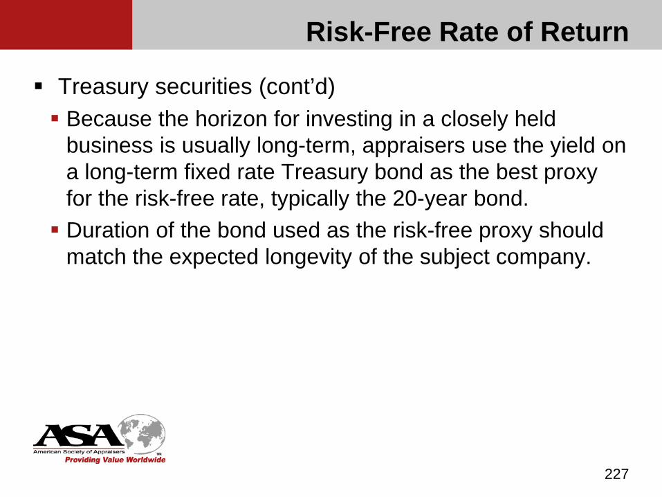
Risk-Free Rate of Return
Treasury securities (cont’d) Because the horizon for investing in a closely held
business is usually long-term, appraisers use the yield on a long-term fixed rate Treasury bond as the best proxy for the risk-free rate, typically the 20-year bond. Duration of the bond used as the risk-free proxy should
match the expected longevity of the subject company.
227
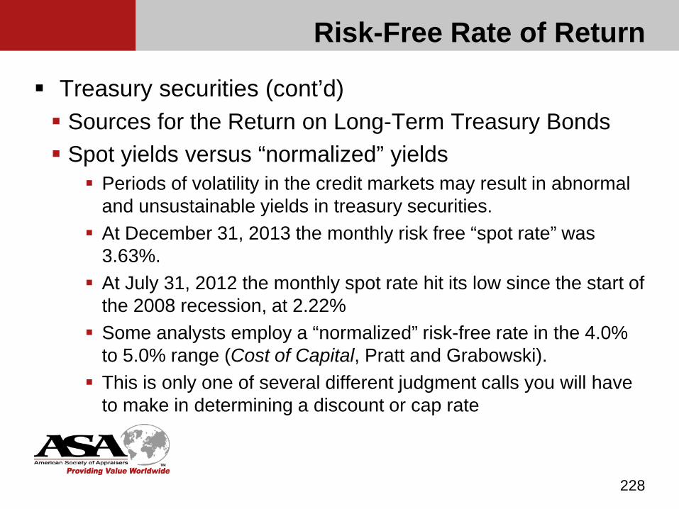
Risk-Free Rate of Return
Treasury securities (cont’d) Sources for the Return on Long-Term Treasury Bonds Spot yields versus “normalized” yields
Periods of volatility in the credit markets may result in abnormal and unsustainable yields in treasury securities.
At December 31, 2013 the monthly risk free “spot rate” was 3.63%.
At July 31, 2012 the monthly spot rate hit its low since the start of the 2008 recession, at 2.22%
Some analysts employ a “normalized” risk-free rate in the 4.0% to 5.0% range (Cost of Capital, Pratt and Grabowski).
This is only one of several different judgment calls you will have to make in determining a discount or cap rate
228
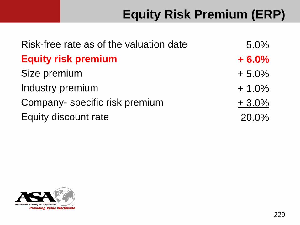
229
Risk-free rate as of the valuation date Equity risk premiumSize premiumIndustry premiumCompany- specific risk premiumEquity discount rate
5.0%+ 6.0%+ 5.0%+ 1.0%+ 3.0%20.0%
Equity Risk Premium (ERP)

Equity Risk Premium (ERP)
The equity risk premium is the rate of return investors receive as compensation for the risk of equities in excess of the rate of return received on the risk-free security.
The general formula for the equity risk premium is:
ERPm = E(Rm) – Rf
ERPm = Risk premium for the equity “market” (ERP) E(Rm) = Expected return on the equity “market” Rf = Risk-free rate of return
230
Equity Risk Premium (ERP)
The ERP is a forward-looking concept. It is based on the expected excess return on the stock market during the term of the investment and should be reflective of what the ERP will be in the future. Forward-looking ERP is unobservable ERP is often estimated by using either
(1) historical realized returns or (2) forward-looking estimates.
231

Equity Risk Premium (ERP)
Historical realized ERP Assumes that the historical differential between stocks and
government bond returns is a relatively stable indicator of investor willingness to assume the risk associated with equities. Advantages of the historical realized ERP
• The data are objective and easy to find.• It conforms to the belief that historical returns may be the best
indicator of future returns.• It is easier to explain what returns were historically realized in the
market than either what returns should have been expected or are projected to occur.
• The use of historical data is widely accepted and the most common method used in the business valuation community.
232
Equity Risk Premium (ERP)
Historical realized ERP Disadvantages of the historical realized ERP
• The past may not reflect the future.• Different measurement periods produce significantly different
results. • Research suggests actual historical realized returns were
different from the returns that were expected.
233
Equity Risk Premium (ERP)
Forward-looking ERP Assumes that an analyst can make a better projection of
the relative risk and return of equities Forward-looking ERP methods include (1) supply-side
models, (2) projections by brokerage firms and economic consulting firms, and (3) surveys of financial professionals and academics. Main advantage of forward-looking ERP: It is
theoretically closer to what we are actually seeking
234
Equity Risk Premium (ERP) (p 122)
A commonly used source for the historical realized ERP had been the Stocks, Bonds, Bills, and Inflation Yearbook (SBBI), last published in 2013 (data through 2012) First published by Ibbotson Associates in 1983 Previously published by Morningstar, Inc. Beginning in 1999, SBBI information is provided in
the SBBI Classic Edition Yearbook and had been in the SBBI Valuation Edition Yearbook
Beginning with 2014 (data through 2013), is now published by Duff & Phelps’ Valuation Handbook and is referred to as “CRSP” data (Center for Research in Security Prices)
235

Equity Risk Premium (ERP)
CRSP ERP (cont’d) Historical market data on the stock market and
government bonds since 1926. Represents the beginning of a new economic cycle brought on
by the Great Depression. The original source for the data is the Center for Research in Security Prices (CRSP).
Calculated as the arithmetic mean of the total return on the stock market less the arithmetic mean of the income-only return on long-term government bonds measured over the same time horizon.
236
Equity Risk Premium (ERP)
CRSP ERP (cont’d) ERPm = E(Rm) – Rf = Average Total Return on the
Market for X years minus the Average Income Return on Long-Term Government Bonds for X years CRSP uses the S&P 500 as its benchmark for the stock
market returns (Rm)
237
Equity Risk Premium (ERP)
CRSP ERP (cont’d) S&P 500
The S&P 500 includes 500 leading companies in 88 leading industries of the U.S. economy and is considered a large company index.
The S&P 500 is capitalization-weighted—The stock prices of the 500 companies are averaged, but the average is weighted by market capitalization, which is the dollar value of a company's outstanding common shares.
238
Equity Risk Premium (ERP)
CRSP ERP (cont’d) S&P 500 (cont’d)
The S&P 500 covers approximately 75% of the U.S. equities market (based on market capitalization) and is considered to be a proxy for the total stock market.
Later editions of SBBI also show alternative measures of broad stock market performance that show different returns than the S&P 500 (see outline)
239

Equity Risk Premium (ERP)
CRSP ERP (cont’d) CRSP provides equity risk premium data based on 30-
day Treasury bills, 5-year Treasury bonds, and 20-year Treasury bonds Since the life of a company is often considered to be
infinite, most business valuation analysts, as well as CRSP, consider the long-horizon ERP based on the 20-year Treasury bond to be appropriate for business valuations.
240

Equity Risk Premium (ERP)
CRSP ERP (cont’d) The total return on Treasury securities has three
components: Income return—portion of the total return from the bond’s coupon
payment, or cash flow Capital appreciation (or depreciation)—change in the price of the
bond over time Reinvestment return—monthly returns reinvested in a similar
bond for the remainder of the bond’s term
241
Equity Risk Premium (ERP)
CRSP ERP (cont’d) The ERP should be calculated by subtracting the long-
term average of the income return only on long-term Treasury bonds from the long-term average stock market return. The capital appreciation and reinvestment returns are
subject to risk from unexpected changes in bond yields, defeating the purpose of trying to identify the most “risk-free” security.
242
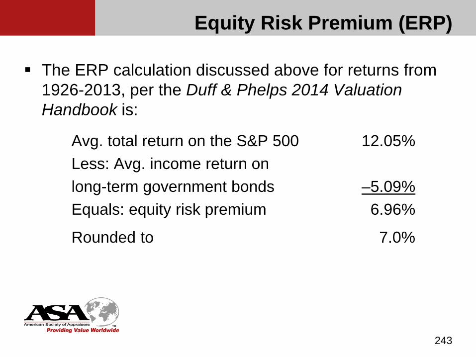
Equity Risk Premium (ERP)
The ERP calculation discussed above for returns from 1926-2013, per the Duff & Phelps 2014 Valuation Handbook is:
Avg. total return on the S&P 500 12.05%Less: Avg. income return onlong-term government bonds –5.09%Equals: equity risk premium 6.96%
Rounded to 7.0%
243
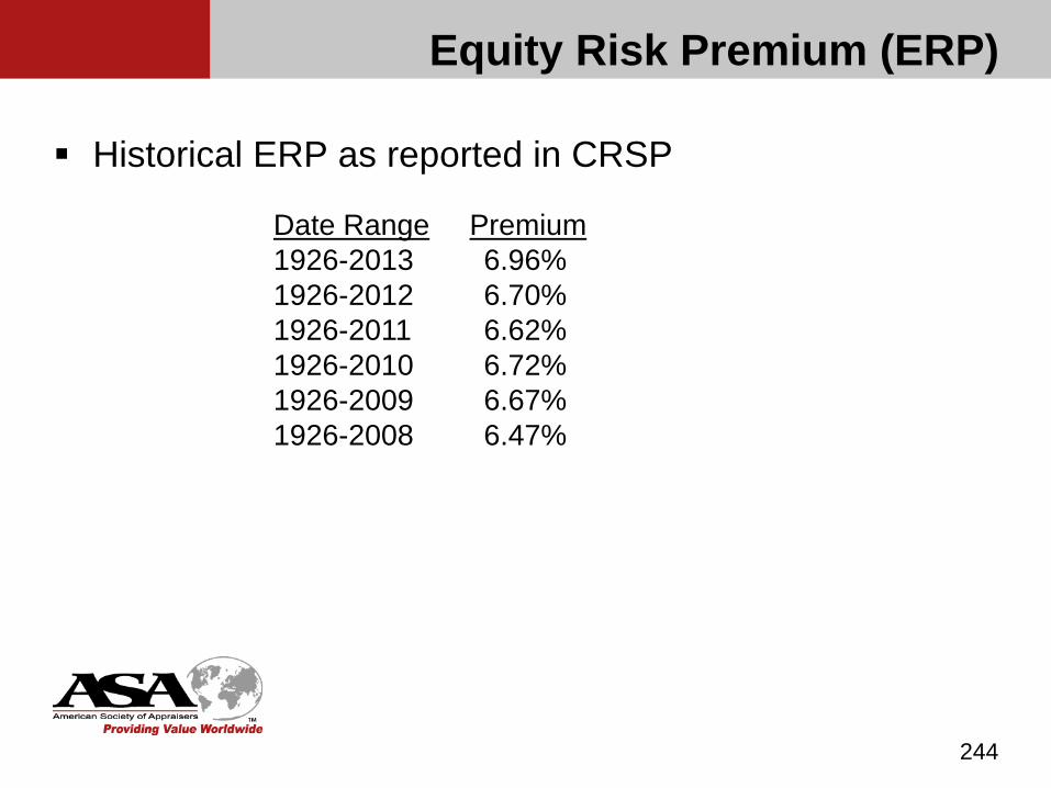
Equity Risk Premium (ERP)
Historical ERP as reported in CRSP
244
Date Range Premium1926-2013 6.96%1926-2012 6.70%1926-2011 6.62%1926-2010 6.72%1926-2009 6.67%1926-2008 6.47%
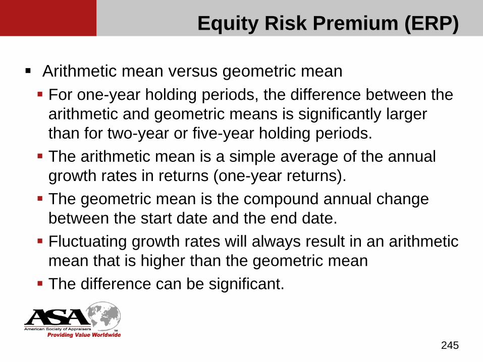
Equity Risk Premium (ERP)
Arithmetic mean versus geometric mean For one-year holding periods, the difference between the
arithmetic and geometric means is significantly larger than for two-year or five-year holding periods. The arithmetic mean is a simple average of the annual
growth rates in returns (one-year returns). The geometric mean is the compound annual change
between the start date and the end date. Fluctuating growth rates will always result in an arithmetic
mean that is higher than the geometric mean The difference can be significant.
245
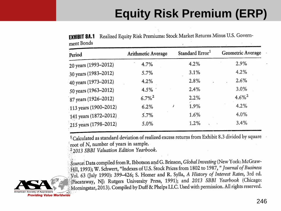
Equity Risk Premium (ERP)
246

Equity Risk Premium (ERP)
Challenges to the traditional ERP reported by CRSP Holding periods
The CRSP ERP is calculated based on one year holding period returns.
Lower ERPs result from using the same data but assuming multiple period returns
Because the multi-period ERP’s are computed based on the geometric average
247

Equity Risk Premium (ERP)
248

Equity Risk Premium (ERP)
Challenges to the traditional ERP reported by CRSP Use of the historical realized ERP is predicated on the
assumption that past patterns are reflective of current investor expectations. This presumed relationship may or may not hold true. A number of academic studies cast doubt on the basic
logic of using historical returns as a basis for quantifying expected returns. This is based on the observation that the historical realized ERP is higher than what can be explained by economic theory.
249
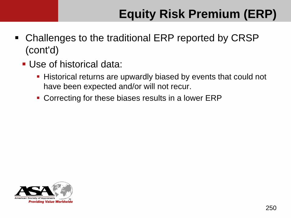
Equity Risk Premium (ERP)
Challenges to the traditional ERP reported by CRSP (cont'd) Use of historical data:
Historical returns are upwardly biased by events that could not have been expected and/or will not recur.
Correcting for these biases results in a lower ERP
250
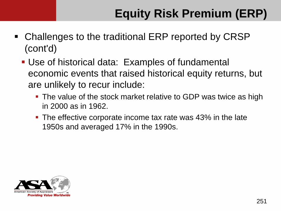
Equity Risk Premium (ERP)
Challenges to the traditional ERP reported by CRSP (cont'd) Use of historical data: Examples of fundamental
economic events that raised historical equity returns, but are unlikely to recur include: The value of the stock market relative to GDP was twice as high
in 2000 as in 1962. The effective corporate income tax rate was 43% in the late
1950s and averaged 17% in the 1990s.
251

Equity Risk Premium (ERP)
Challenges to the traditional ERP reported by CRSP (cont'd) Use of historical data: Examples of fundamental
economic events that raised historical equity returns, but are unlikely to recur include: Equity investments can now be held in tax-free or tax-deferred
accounts, which did not exist in the 1950s and 1960s. Low real rates on bonds during the immediate post-World War II
period contributed to higher equity returns. Alternative estimates of the ERP: 2.9% to 4.5% (see outline)
252
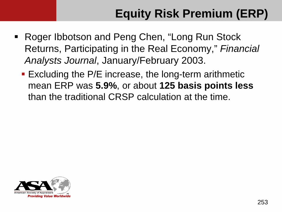
Equity Risk Premium (ERP)
Roger Ibbotson and Peng Chen, “Long Run Stock Returns, Participating in the Real Economy,” Financial Analysts Journal, January/February 2003. Excluding the P/E increase, the long-term arithmetic
mean ERP was 5.9%, or about 125 basis points lessthan the traditional CRSP calculation at the time.
253

Equity Risk Premium (ERP) (p 128)
Supply side ERP Intended to measure a forward-looking ERP Use fundamental information, such as earnings, dividend,
or overall economic productivity CRSP now presents the supply-side ERP based on the
Ibbotson and Chen model. Breaks historical realized equity returns into (1) inflation, (2)
income return, (3) growth in real earnings per share, and (4) growth in P/E ratio.
The CRSP supply-side ERP excludes the growth in the P/E ratio.
254
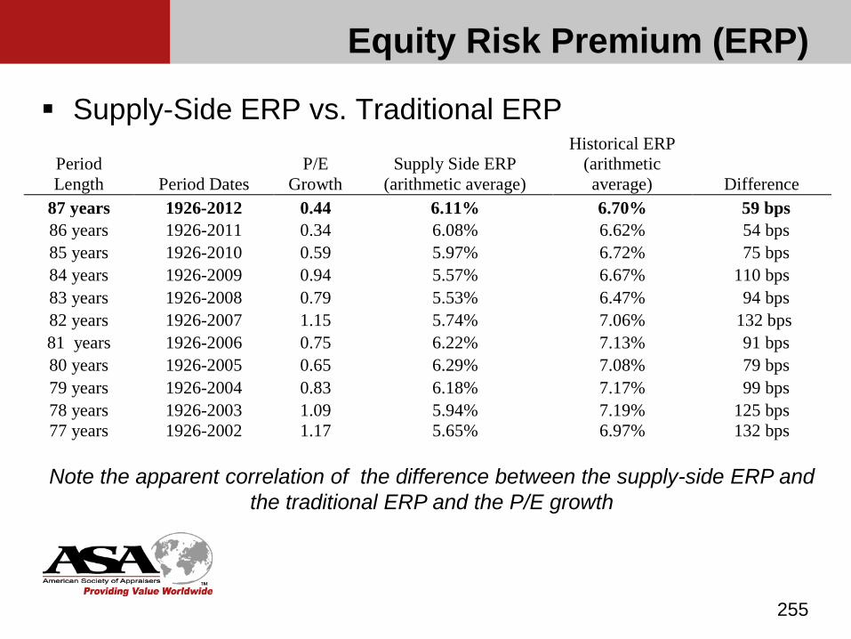
Equity Risk Premium (ERP)
Supply-Side ERP vs. Traditional ERP
255
Note the apparent correlation of the difference between the supply-side ERP and the traditional ERP and the P/E growth
Period Length Period Dates
P/E Growth
Supply Side ERP (arithmetic average)
Historical ERP (arithmetic average) Difference
87 years 1926-2012 0.44 6.11% 6.70% 59 bps 86 years 1926-2011 0.34 6.08% 6.62% 54 bps 85 years 1926-2010 0.59 5.97% 6.72% 75 bps 84 years 1926-2009 0.94 5.57% 6.67% 110 bps 83 years 1926-2008 0.79 5.53% 6.47% 94 bps 82 years 1926-2007 1.15 5.74% 7.06% 132 bps 81 years 1926-2006 0.75 6.22% 7.13% 91 bps 80 years 1926-2005 0.65 6.29% 7.08% 79 bps 79 years 1926-2004 0.83 6.18% 7.17% 99 bps 78 years 1926-2003 1.09 5.94% 7.19% 125 bps 77 years 1926-2002 1.17 5.65% 6.97% 132 bps
Equity Risk Premium (ERP)
Supply side ERP (cont’d) Several other studies and survey data exist – refer to the
course manual
256
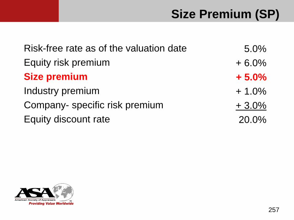
257
Risk-free rate as of the valuation date Equity risk premiumSize premiumIndustry premiumCompany- specific risk premiumEquity discount rate
5.0%+ 6.0%+ 5.0%+ 1.0%+ 3.0%20.0%
Size Premium (SP)
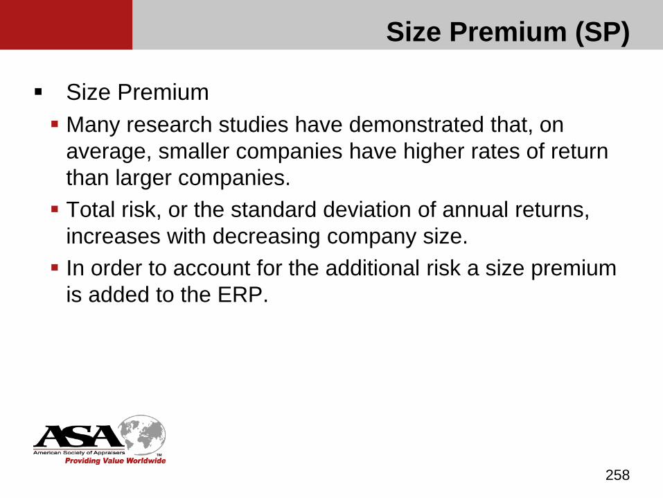
Size Premium (SP)
Size Premium Many research studies have demonstrated that, on
average, smaller companies have higher rates of return than larger companies. Total risk, or the standard deviation of annual returns,
increases with decreasing company size. In order to account for the additional risk a size premium
is added to the ERP.
258
Size Premium (SP)
The two most commonly used sources of empirical data for the size premium CRSP Size Premium Duff and Phelps Risk Premium Study
259

Size Premium (SP)
CRSP Size Deciles CRSP presents information that analyzes the size effect
across 10 deciles of the stock market. Both the average returns and the total risk increase as
one moves from the decile containing the largest companies (Decile 1) to the decile containing the smallest companies (Decile 10).
260

Size Premium (SP)
CRSP Size Deciles (cont’d) In addition to providing historical realized returns for each
decile, CRSP calculates the excess return due purely to size (“beta-adjusted” size premium), rather than incorporating both size and industry considerations as the traditional CRSP Small Company Stock Premium does.
261
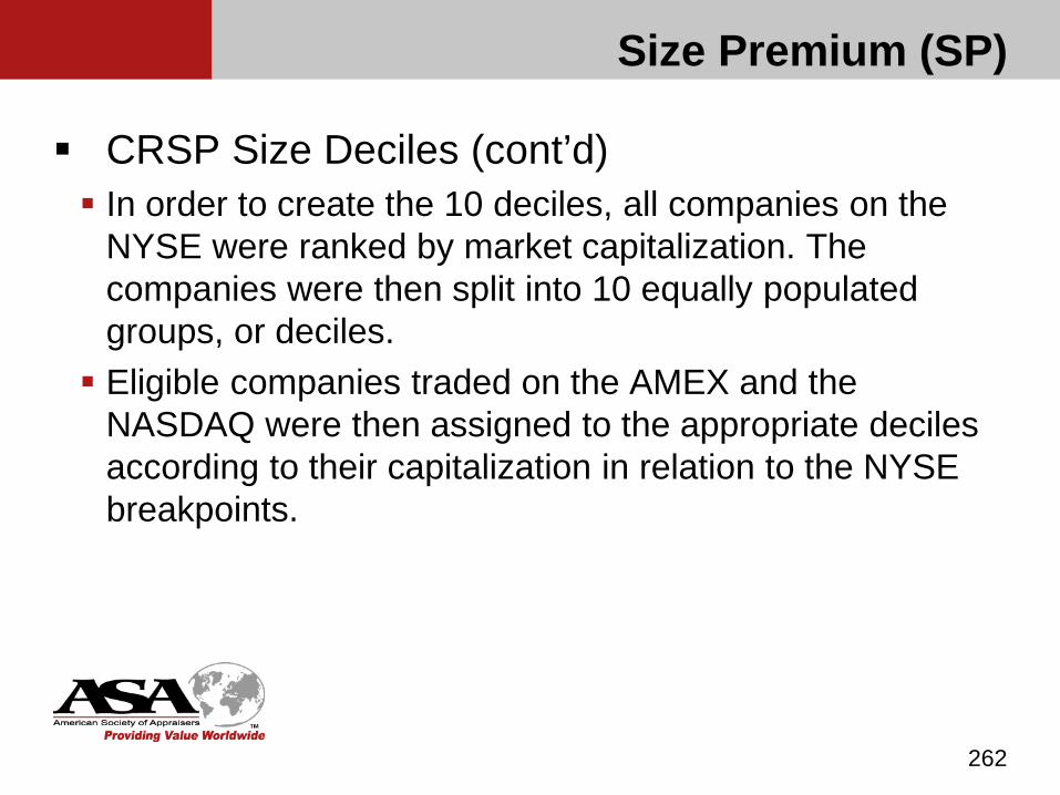
Size Premium (SP)
CRSP Size Deciles (cont’d) In order to create the 10 deciles, all companies on the
NYSE were ranked by market capitalization. The companies were then split into 10 equally populated groups, or deciles. Eligible companies traded on the AMEX and the
NASDAQ were then assigned to the appropriate decilesaccording to their capitalization in relation to the NYSE breakpoints.
262
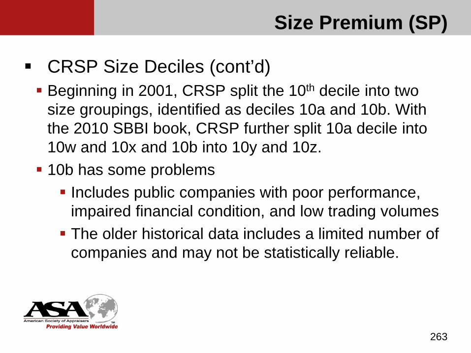
Size Premium (SP)
CRSP Size Deciles (cont’d) Beginning in 2001, CRSP split the 10th decile into two
size groupings, identified as deciles 10a and 10b. With the 2010 SBBI book, CRSP further split 10a decile into 10w and 10x and 10b into 10y and 10z. 10b has some problems Includes public companies with poor performance,
impaired financial condition, and low trading volumes The older historical data includes a limited number of
companies and may not be statistically reliable.
263
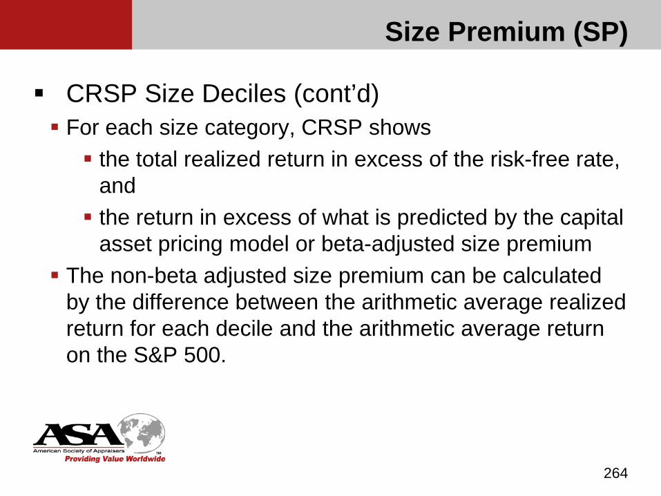
Size Premium (SP)
CRSP Size Deciles (cont’d) For each size category, CRSP shows the total realized return in excess of the risk-free rate,
and the return in excess of what is predicted by the capital
asset pricing model or beta-adjusted size premium The non-beta adjusted size premium can be calculated
by the difference between the arithmetic average realized return for each decile and the arithmetic average return on the S&P 500.
264

Size Premium (SP)
CRSP Size Deciles (cont’d) According to CRSP, in the Build-up model, the beta-
adjusted size premium should be used.
265
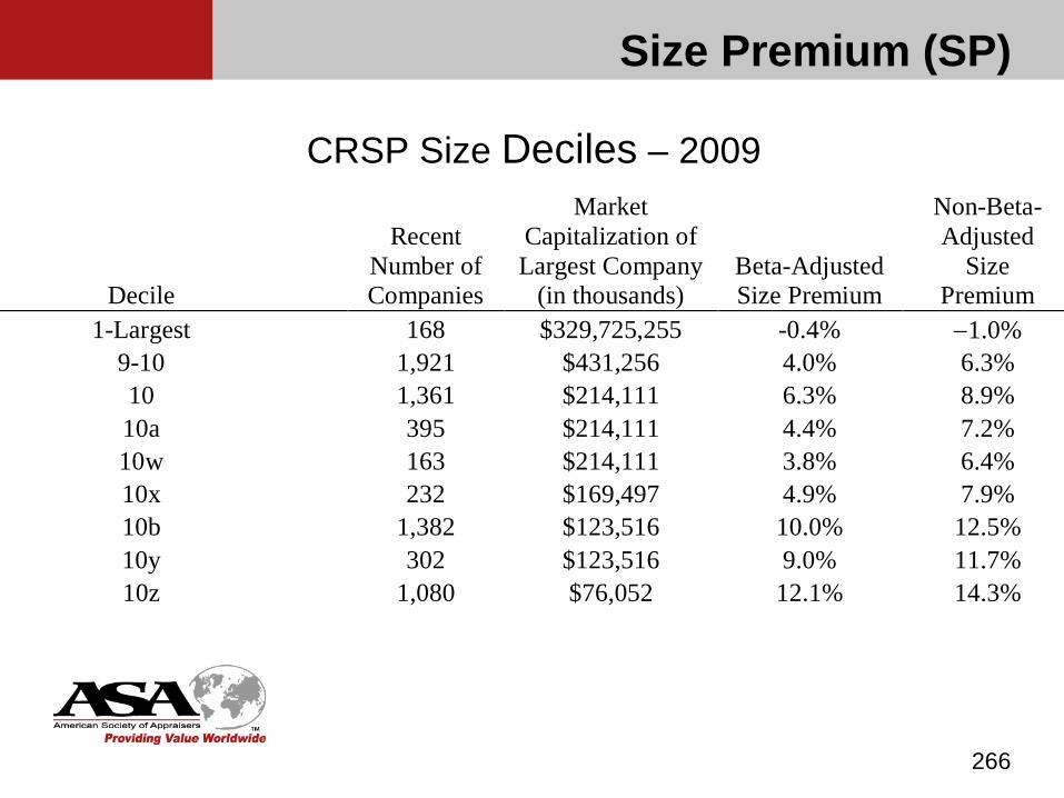
Size Premium (SP)
CRSP Size Deciles – 2009
266
Decile
Recent Number of Companies
Market Capitalization of Largest Company
(in thousands) Beta-Adjusted Size Premium
Non-Beta-Adjusted
Size Premium
1-Largest 168 $329,725,255 -0.4% −1.0% 9-10 1,921 $431,256 4.0% 6.3% 10 1,361 $214,111 6.3% 8.9% 10a 395 $214,111 4.4% 7.2% 10w 163 $214,111 3.8% 6.4% 10x 232 $169,497 4.9% 7.9% 10b 1,382 $123,516 10.0% 12.5% 10y 302 $123,516 9.0% 11.7% 10z 1,080 $76,052 12.1% 14.3%
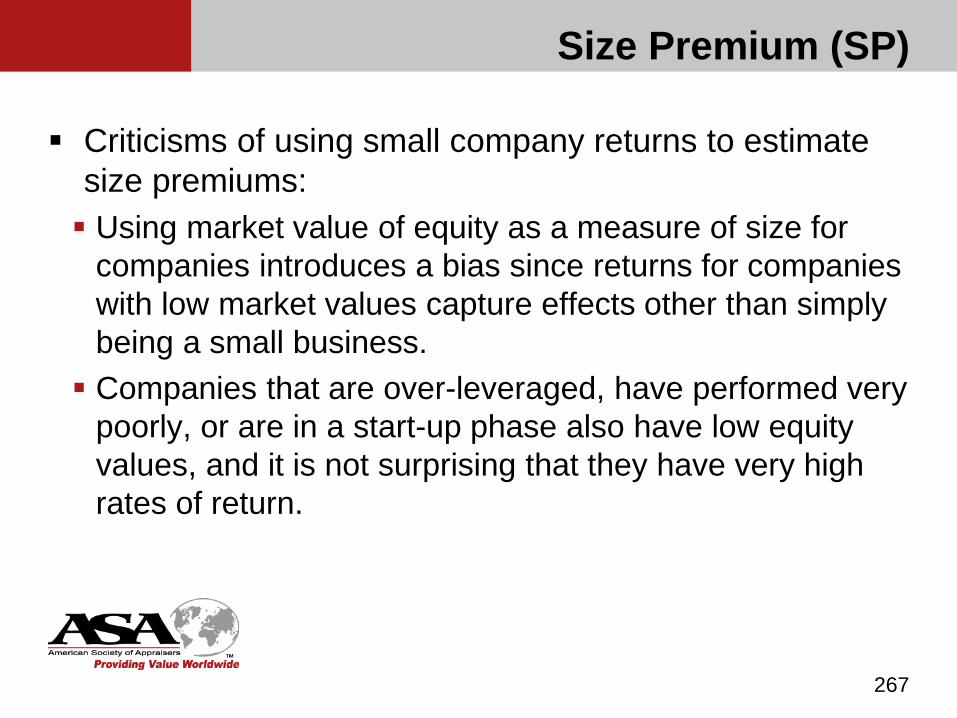
Size Premium (SP)
Criticisms of using small company returns to estimate size premiums: Using market value of equity as a measure of size for
companies introduces a bias since returns for companies with low market values capture effects other than simply being a small business. Companies that are over-leveraged, have performed very
poorly, or are in a start-up phase also have low equity values, and it is not surprising that they have very high rates of return.
267
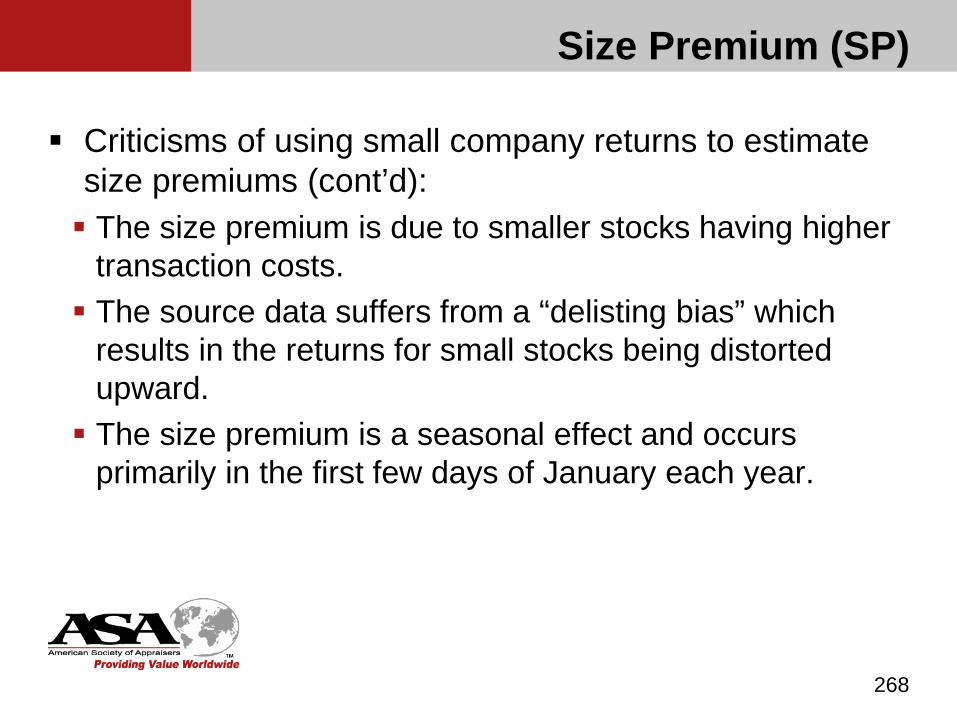
Size Premium (SP)
Criticisms of using small company returns to estimate size premiums (cont’d): The size premium is due to smaller stocks having higher
transaction costs. The source data suffers from a “delisting bias” which
results in the returns for small stocks being distorted upward. The size premium is a seasonal effect and occurs
primarily in the first few days of January each year.
268

Exercise 8-1
269
BUILD UP METHOD (CRSP)Using information provided in Exhibit 8-2 (at the end of Chapter 8), calculate the equity discount rate for Spring Hill Furniture based on the build-up method, assuming the expected ERP and a company specific risk premium of 4%. Assume the company’s size places it in subdecile 10b and do not use an industry risk premium.

Exercise 8-1 SOLUTION
270
Exercise 8-1 SolutionComponent Rate SourceRisk-Free Rate 4.6% 20-Year Treasury Bond Rate
Equity Risk Premium + 6.0% Supply side (forward-looking) ERP
Size Premium + 9.7% Beta Adjusted Size Premia for 10b subdecile
Company-Specific Risk Premium + 4.0% Given
Equity Discount Rate 24.3%
An Alternative to the CRSP Build Up Method Duff & Phelps Risk Premium Reports
271
Duff & Phelps Risk Premium Study (p. 133)
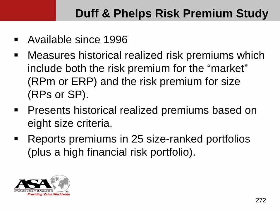
Duff & Phelps Risk Premium Study
Available since 1996 Measures historical realized risk premiums which
include both the risk premium for the “market” (RPm or ERP) and the risk premium for size (RPs or SP).
Presents historical realized premiums based on eight size criteria.
Reports premiums in 25 size-ranked portfolios (plus a high financial risk portfolio).
272
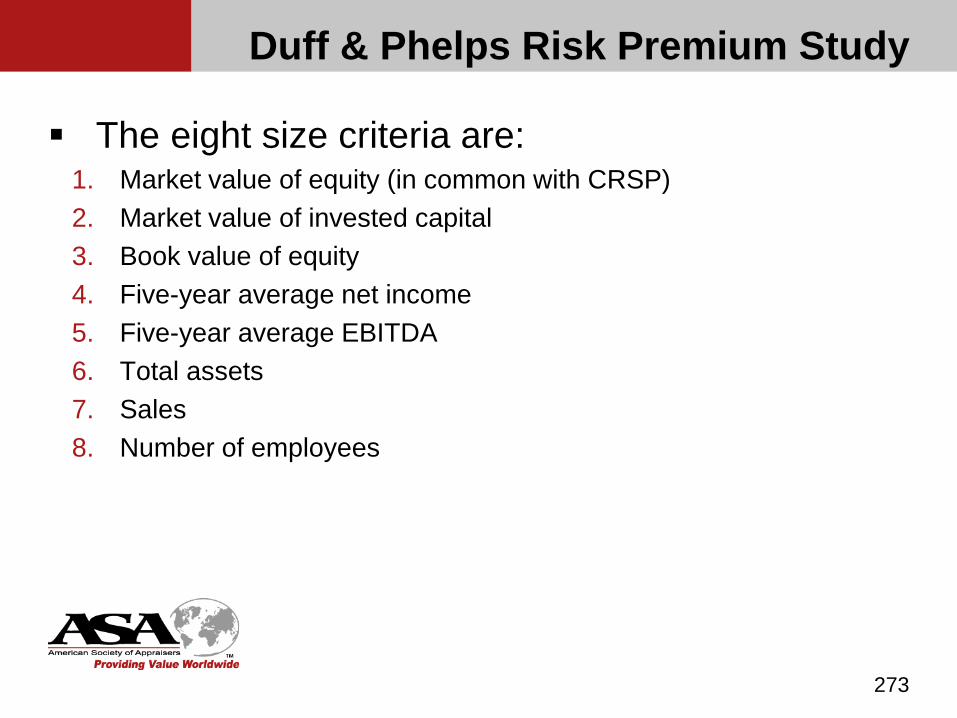
Duff & Phelps Risk Premium Study
The eight size criteria are:1. Market value of equity (in common with CRSP)2. Market value of invested capital3. Book value of equity4. Five-year average net income 5. Five-year average EBITDA6. Total assets 7. Sales8. Number of employees
273

Duff & Phelps Risk Premium Study
The table below presents a further breakdown of the metrics of the companies that comprise the 25th portfolio. The two metrics that are based on market value of equity are not shown; dollars are in millions. Some are fairly small (i. e., sales < $1.7 million; 5-yr average net income <$200k)
274
BOOK VALUE
OF EQUITY
5-YR AVG
NET INC
TOTAL
ASSETS
5-YR AVG
EBITDA
SALES # OF
EMPLOYEES
LARGEST 149.763 8.816 274.802 36.979 266.356 560
MEDIAN 58.803 3.627 104.899 13.698 102.842 233
SMALLEST 4.327 0.190 5.791 0.317 1.671 3

Duff & Phelps Risk Premium Study
It may still be that the subject company’s metrics fall below these ranges. “In such cases, it may be appropriate to extrapolate to smaller sizes using the regression equations. As a general rule, extrapolating a statistical relationship far beyond the range of the data used in the statistical analysis is not recommended.
“We {D&P} do not recommend extrapolating in cases where all size measures of the subject are less than the smallest company comprising the 25th portfolio, and one should never use those size measures for which the subject company’s size is equal to zero or negative.”
275
Duff & Phelps Risk Premium Study
The analyst does not need to use all eight measures of size when estimating the cost of equity using the Duff & Phelps data.
“When using the Size Study, the minimum number of size measures required is one.”
276
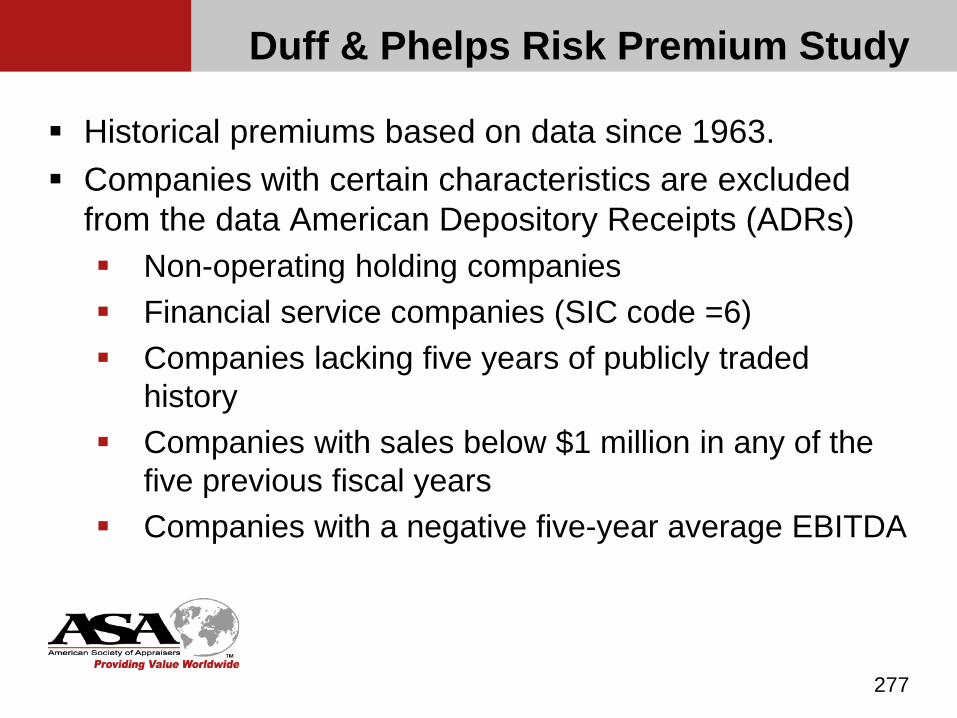
Duff & Phelps Risk Premium Study
Historical premiums based on data since 1963. Companies with certain characteristics are excluded
from the data American Depository Receipts (ADRs) Non-operating holding companies Financial service companies (SIC code =6) Companies lacking five years of publicly traded
history Companies with sales below $1 million in any of the
five previous fiscal years Companies with a negative five-year average EBITDA
277
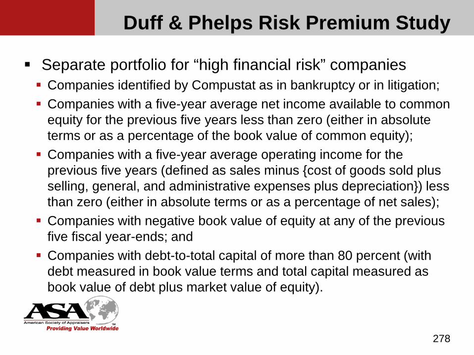
Duff & Phelps Risk Premium Study
Separate portfolio for “high financial risk” companies Companies identified by Compustat as in bankruptcy or in litigation; Companies with a five-year average net income available to common
equity for the previous five years less than zero (either in absolute terms or as a percentage of the book value of common equity);
Companies with a five-year average operating income for the previous five years (defined as sales minus {cost of goods sold plus selling, general, and administrative expenses plus depreciation}) less than zero (either in absolute terms or as a percentage of net sales);
Companies with negative book value of equity at any of the previous five fiscal year-ends; and
Companies with debt-to-total capital of more than 80 percent (with debt measured in book value terms and total capital measured as book value of debt plus market value of equity).
278

Duff & Phelps Risk Premium Study
The D&P Report differs from the CRSP size premium analysis in several key areas: The period covered by its analysis—The D&P data cover
1963 through the valuation date rather than 1926 forward, which is tabulated in the CRSP calculation. The nature of the calculated ERP—The D&P ERP
includes both the ERP for large company stocks and the size premium.
279

Duff & Phelps Risk Premium Study
The D&P Report differs from the CRSP size premium analysis in several key areas (cont’d): The number of stratifications of size—The D&P Report contains 25;
the CRSP study contains 10. The D&P Report calculates a “smoothed” average historical ERP
using a regression analysis with the average historical equity risk premium as dependent variable and the logarithm of the average sorting criteria as independent variable (converted into a base-10 logarithm).
280
Duff & Phelps Risk Premium Study
The D&P Report differs from the CRSP size premium analysis in several key areas (cont’d): The D&P Report provides the average debt to market value of
invested capital (MVIC) ratio for each portfolio
281
Duff & Phelps Risk Premium Study
The D&P Report has two separate data sets for use, depending on the methodology used to develop a discount rate. Exhibits A-1 through A-8 of the D&P Report (the “A Exhibits”) provide
historical risk premiums for use in the Build-up method. Exhibits B-1 though B-8 (the “B Exhibits”) provide premiums over
CAPM data for use in the capital asset pricing model (CAPM).
282
D&P publishes additional tables, which the practitioner should be aware of, but a deeper discussion of which is beyond the scope of this course- C Exhibits – present the data for the 25 portfolios ranked by the
eight measure of size, and presenting three risk characteristics: operating margin, coefficient of variation (“cv”) in operating income margin and cv in return on book equity
D Exhibits – rank the companies not by measures of size, but by accounting measures of profitability: operating margin, cv in operating income margin and cv in return on book equity.
H Exhibits – separate exhibits for high financial risk companies, i.e., losing money, high leverage, in bankruptcy.
283
Duff & Phelps Risk Premium Study

The C Exhibits, D Exhibits and H Exhibits can be useful in estimating specific company risk by observing the returns of companies with these specific risk characteristics (profitability, cv in profitability, financial distress)
284
Duff & Phelps Risk Premium Study

Duff & Phelps Risk Premium Study
The size premium over the risk free rate (A Exhibits) always requires application of the ERP Adjustment whereas
The size premium over the CAPM (B Exhibits) never requires application of the ERP Adjustment because it is already reflected in the CAPM estimate
Exhibit 9-2 contains an excerpt from the D&P reports summarizing how to properly use the data in the several D&P exhibits.
285
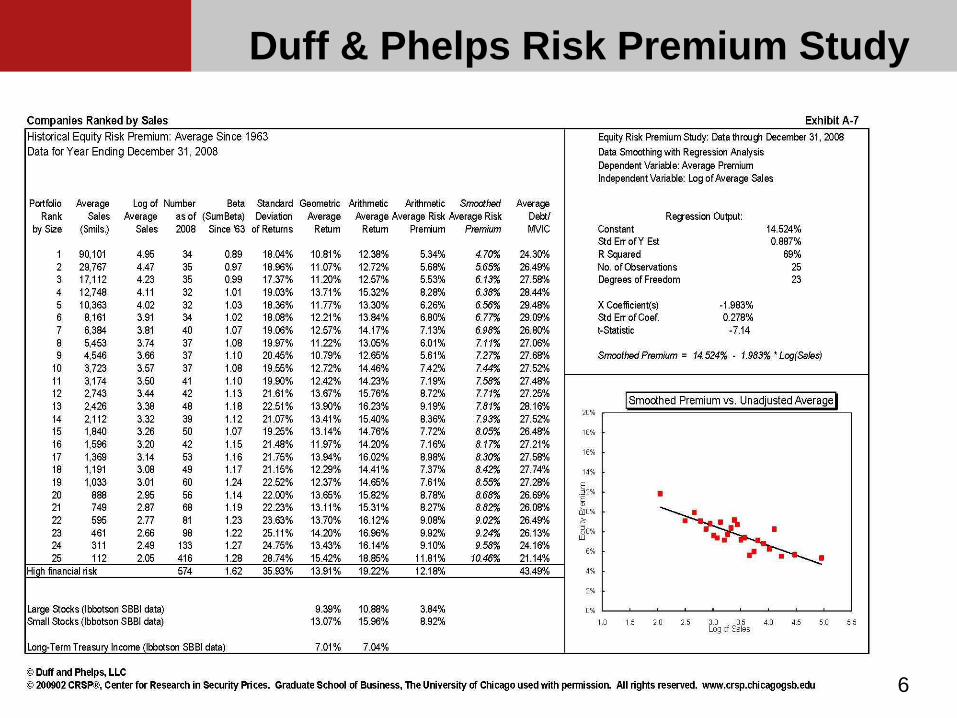
Duff & Phelps Risk Premium Study
286
Duff & Phelps Risk Premium Study
The D&P Report has two separate data sets for use, depending on the methodology used to develop a discount rate. Exhibits B-1 though B-8 of the D&P Report (the “B Exhibits”) provide
premiums over CAPM data for use in the capital asset pricing model (CAPM).
287
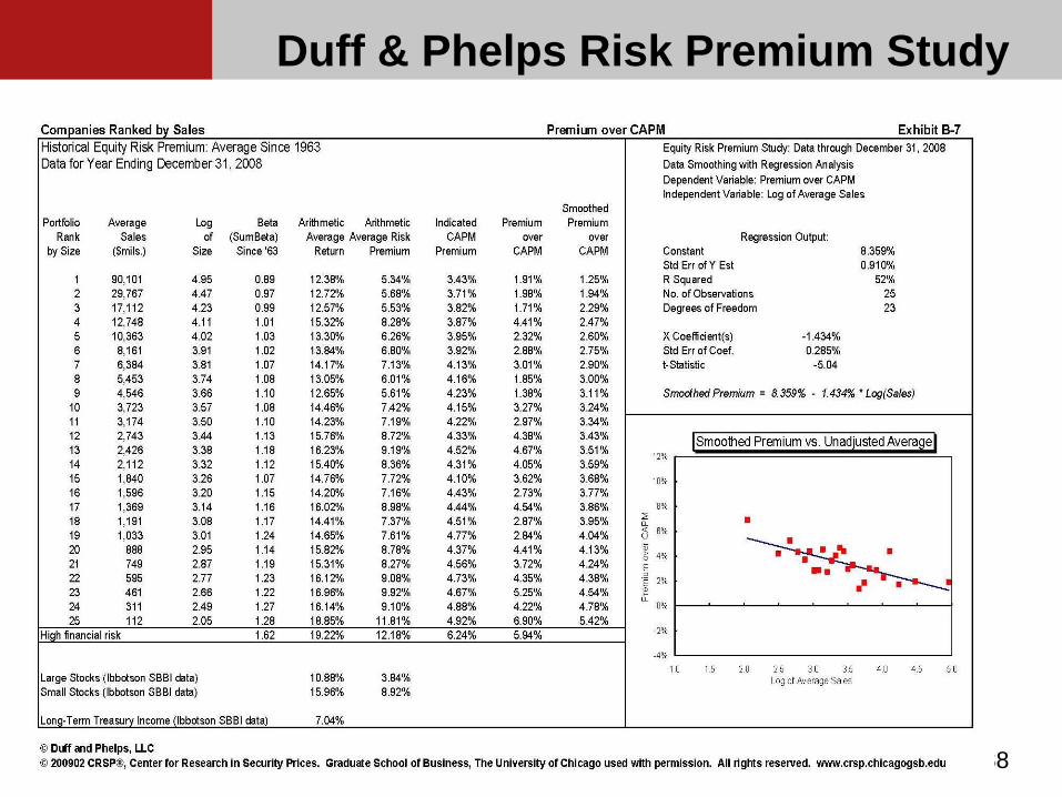
Duff & Phelps Risk Premium Study
288
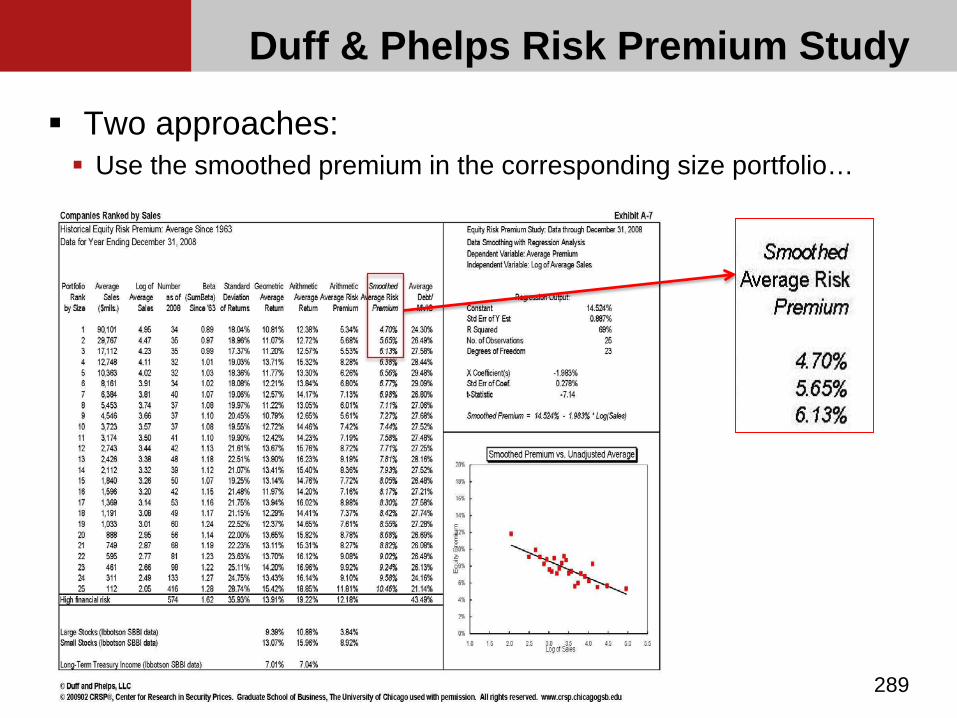
Duff & Phelps Risk Premium Study
Two approaches: Use the smoothed premium in the corresponding size portfolio…
289

Duff & Phelps Risk Premium Study
Two approaches: …Or use the linear regression equation
290
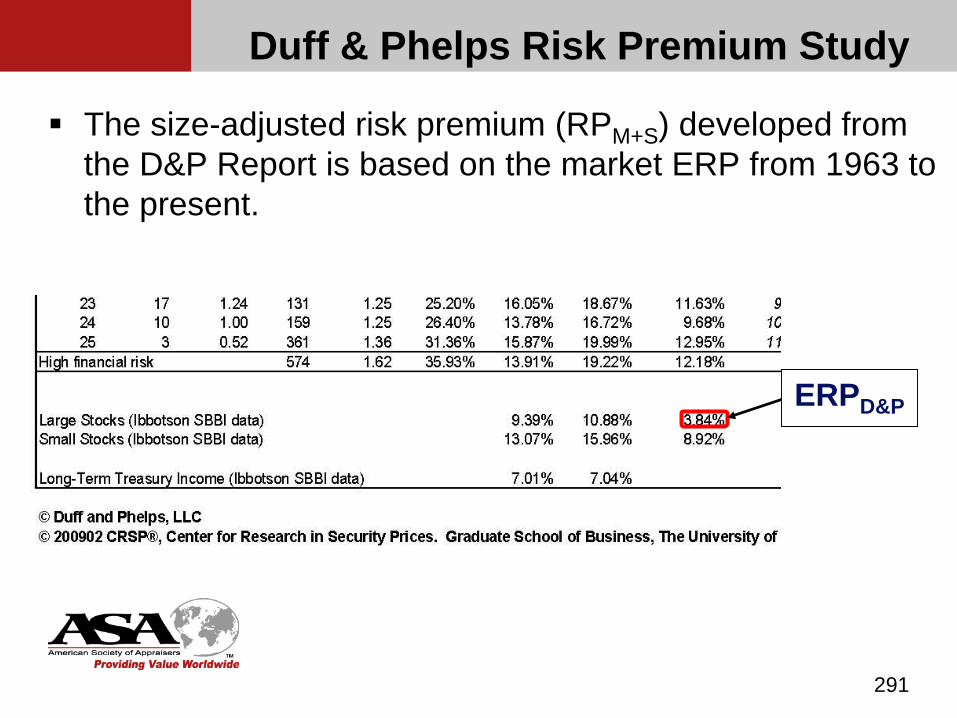
Duff & Phelps Risk Premium Study
The size-adjusted risk premium (RPM+S) developed from the D&P Report is based on the market ERP from 1963 to the present.
291
ERPD&P

Duff & Phelps Risk Premium Study
When using the Duff & Phelps A Exhibits, the RPM+Smust be adjusted for any differences between the historical ERP and the expected future ERP.
For example: The analyst estimates a size-adjusted risk premium of 12.10% from the D&P Report regression equations. The historical ERP implied in the D&P Report is 3.84%. However, the analyst believes the future market ERP will be closer to 5.00%. The size-adjusted risk premium can be further adjusted by adding to it the difference between the expected ERP (5.00%) and the historical ERP (3.84%)
Adjusted RPM+S = 12.10% + (5.00% - 3.84%) = 12.10% + 1.16% = 13.26%
292
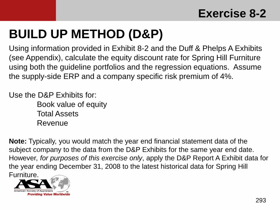
Exercise 8-2
293
BUILD UP METHOD (D&P)Using information provided in Exhibit 8-2 and the Duff & Phelps A Exhibits (see Appendix), calculate the equity discount rate for Spring Hill Furniture using both the guideline portfolios and the regression equations. Assume the supply-side ERP and a company specific risk premium of 4%.
Use the D&P Exhibits for:Book value of equityTotal AssetsRevenue
Note: Typically, you would match the year end financial statement data of the subject company to the data from the D&P Exhibits for the same year end date. However, for purposes of this exercise only, apply the D&P Report A Exhibit data for the year ending December 31, 2008 to the latest historical data for Spring Hill Furniture.

Exercise 8-2 SOLUTION8-2 Using the A Exhibits
a. Estimate size-adjusted ERP$mm Guideline Smoothed Premium
Portfolio 2008 D&PBook value of equity 26.823 25 10.88%Total assets 36.775 25 11.21%Total sales 69.918 25 10.46%
Average premium 10.85%
b. Determine equity discount rateComponent RateRisk-free rate (20-year Treasury bond rate) 4.60%Equity risk premium, adjusted for size (above) 10.85%Adjusted ERP (6.0% forward looking less 3.84% historical) 2.16%Company specific premium (Given) 4.00%
21.61%
294
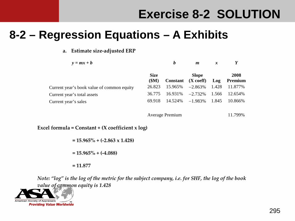
Exercise 8-2 SOLUTION
295
8-2 – Regression Equations – A Exhibitsa. Estimate size-adjusted ERP
y = mx + b b m x Y
Size ($M) Constant
Slope (X coeff) Log
2008 Premium
Current year’s book value of common equity 26.823 15.965% −2.863% 1.428 11.877%
Current year’s total assets 36.775 16.931% −2.732% 1.566 12.654%
Current year’s sales 69.918 14.524% −1.983% 1.845 10.866%
Average Premium 11.799%
Excel formula = Constant + (X coefficient x log)
= 15.965% + (-2.863 x 1.428)
= 15.965% + (-4.088)
= 11.877
Note: “log” is the log of the metric for the subject company, i.e. for SHF, the log of the book value of common equity is 1.428

Exercise 8-2 SOLUTION
296
8-2 – Regression Equations
a. Determine equity discount rate
Component Rate Source Risk-Free Rate 4.6% 20-Year Treasury Bond Rate Equity Risk Premium (Adjusted for Size) + 11.8% From above Adjusted ERP + 2.2% 6.0% forward-looking less 3.8% historical Company-Specific Risk Premium + 4.0% Given Equity Discount Rate 22.6%
Note the difference in the resulting premiums between using the guideline portfolios and the regression equations. This difference illustrates the risk of not capturing the entire size risk premium for smaller companies if the portfolios are used.
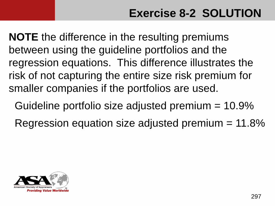
Exercise 8-2 SOLUTION
297
NOTE the difference in the resulting premiums between using the guideline portfolios and the regression equations. This difference illustrates the risk of not capturing the entire size risk premium for smaller companies if the portfolios are used.Guideline portfolio size adjusted premium = 10.9%Regression equation size adjusted premium = 11.8%
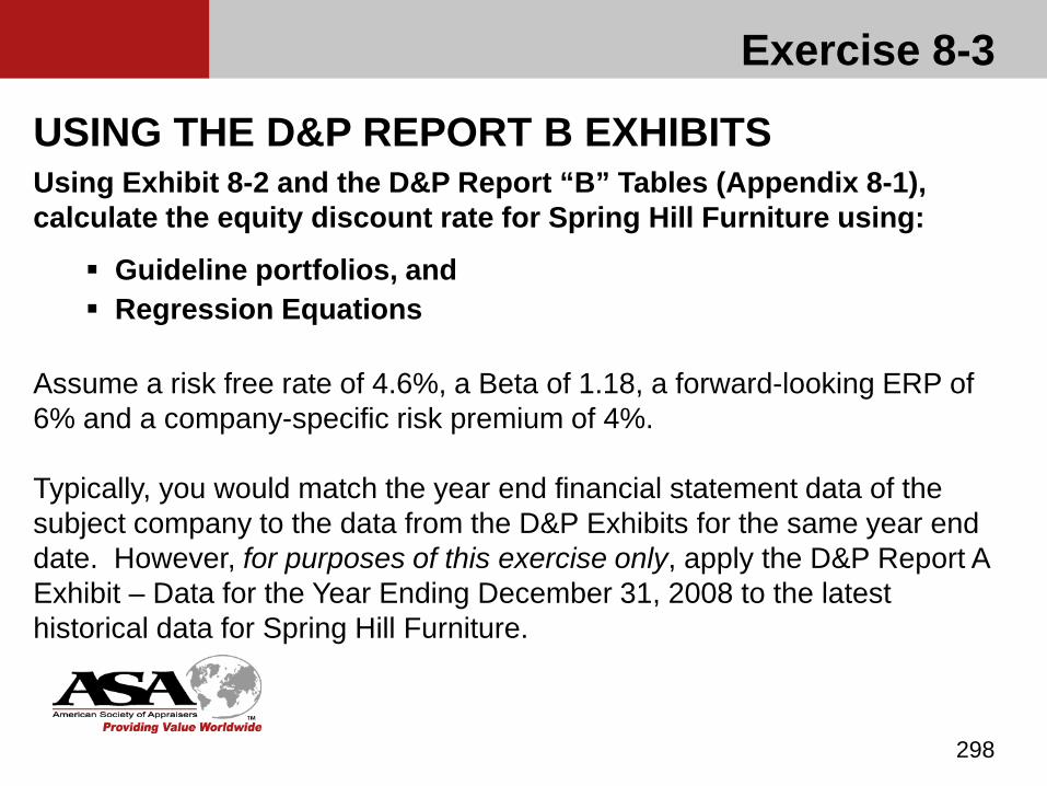
Exercise 8-3
298
USING THE D&P REPORT B EXHIBITSUsing Exhibit 8-2 and the D&P Report “B” Tables (Appendix 8-1), calculate the equity discount rate for Spring Hill Furniture using:
Guideline portfolios, and Regression Equations
Assume a risk free rate of 4.6%, a Beta of 1.18, a forward-looking ERP of 6% and a company-specific risk premium of 4%.
Typically, you would match the year end financial statement data of the subject company to the data from the D&P Exhibits for the same year end date. However, for purposes of this exercise only, apply the D&P Report A Exhibit – Data for the Year Ending December 31, 2008 to the latest historical data for Spring Hill Furniture.
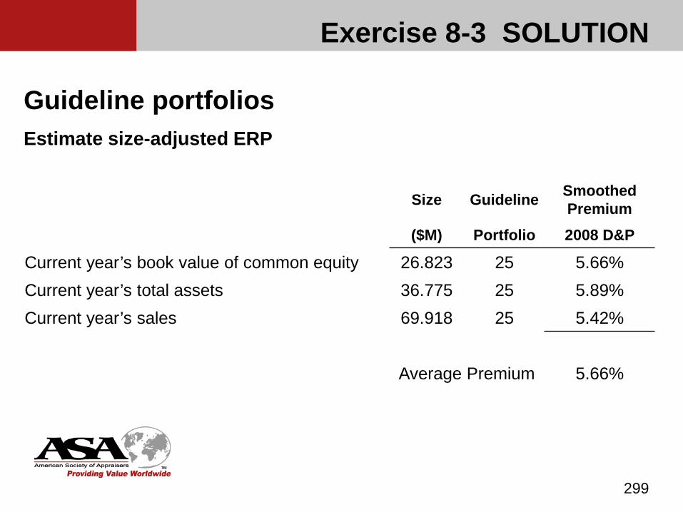
Exercise 8-3 SOLUTION
299
Guideline portfoliosEstimate size-adjusted ERP
Size Guideline SmoothedPremium
($M) Portfolio 2008 D&P
Current year’s book value of common equity 26.823 25 5.66%Current year’s total assets 36.775 25 5.89%Current year’s sales 69.918 25 5.42%
Average Premium 5.66%
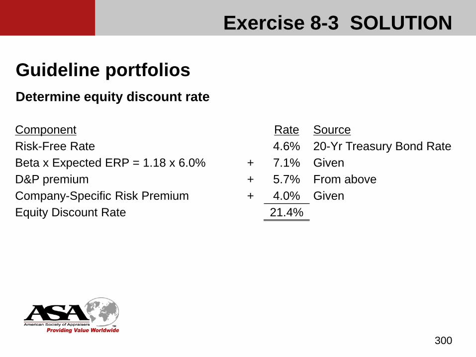
Exercise 8-3 SOLUTION
300
Guideline portfoliosDetermine equity discount rate
Component Rate SourceRisk-Free Rate 4.6% 20-Yr Treasury Bond RateBeta x Expected ERP = 1.18 x 6.0% + 7.1% GivenD&P premium + 5.7% From aboveCompany-Specific Risk Premium + 4.0% GivenEquity Discount Rate 21.4%
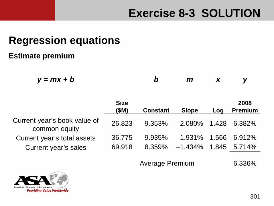
Exercise 8-3 SOLUTION
301
Regression equationsEstimate premium
y = mx + b b m x y
Size($M) Constant Slope Log
2008 Premium
Current year’s book value of common equity
26.823 9.353% −2.080% 1.428 6.382%
Current year’s total assets 36.775 9.935% −1.931% 1.566 6.912%Current year’s sales 69.918 8.359% −1.434% 1.845 5.714%
Average Premium 6.336%
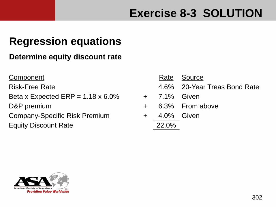
Exercise 8-3 SOLUTION
302
Regression equationsDetermine equity discount rate
Component Rate SourceRisk-Free Rate 4.6% 20-Year Treas Bond RateBeta x Expected ERP = 1.18 x 6.0% + 7.1% GivenD&P premium + 6.3% From aboveCompany-Specific Risk Premium + 4.0% GivenEquity Discount Rate 22.0%

Re-levering the ERP (page 146)
The equity risk premiums (and size-adjusted premiums) developed in the Build-up model with CRSP and D&P Report data reflect the leverage used by the companies in the studies. The subject company may have a different debt structure and, therefore, a different risk profile.
Un-levering the ERP removes the financial risk from the observed data. The unlevered ERP measures pure operating risk without the effect of leverage.
303

Re-levering the ERP
Some practitioners re-lever ERPs to adjust for the subject company’s use of leverage and the associated financial risk. This typically is appropriate only in those circumstances where the assumption is that the capital structure of the subject company will be different than that of the general market.
304

Re-levering the ERP
Since most analysts use CRSP and D&P Report data to estimate the ERP, it is important to know what the authors of those studies say about this topic. D&P suggests the premium derived from its data may be
re-levered if the analyst suspects that the risk profile of the subject company differs from that of the companies in the D&P Report data due to leverage. CRSP is silent.
305
Re-levering the ERP
The concept and methodologies for un-levering and re-levering will be discussed in more detail in the next chapter in the context of re-levering betas for the Capital Asset Pricing Model.
306
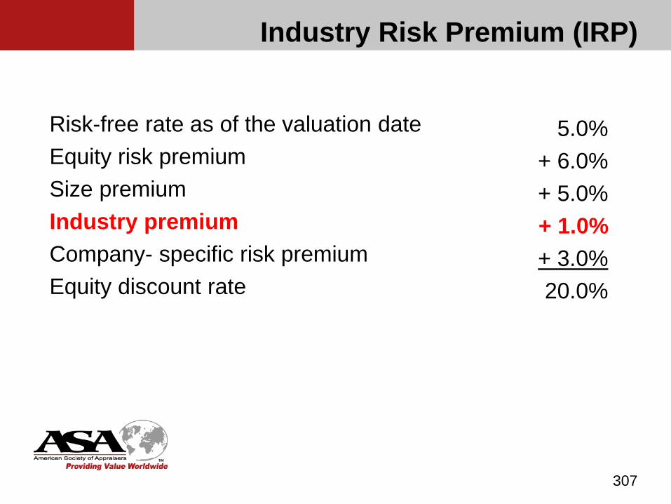
307
Risk-free rate as of the valuation date Equity risk premiumSize premiumIndustry premiumCompany- specific risk premiumEquity discount rate
5.0%+ 6.0%+ 5.0%+ 1.0%+ 3.0%20.0%
Industry Risk Premium (IRP)
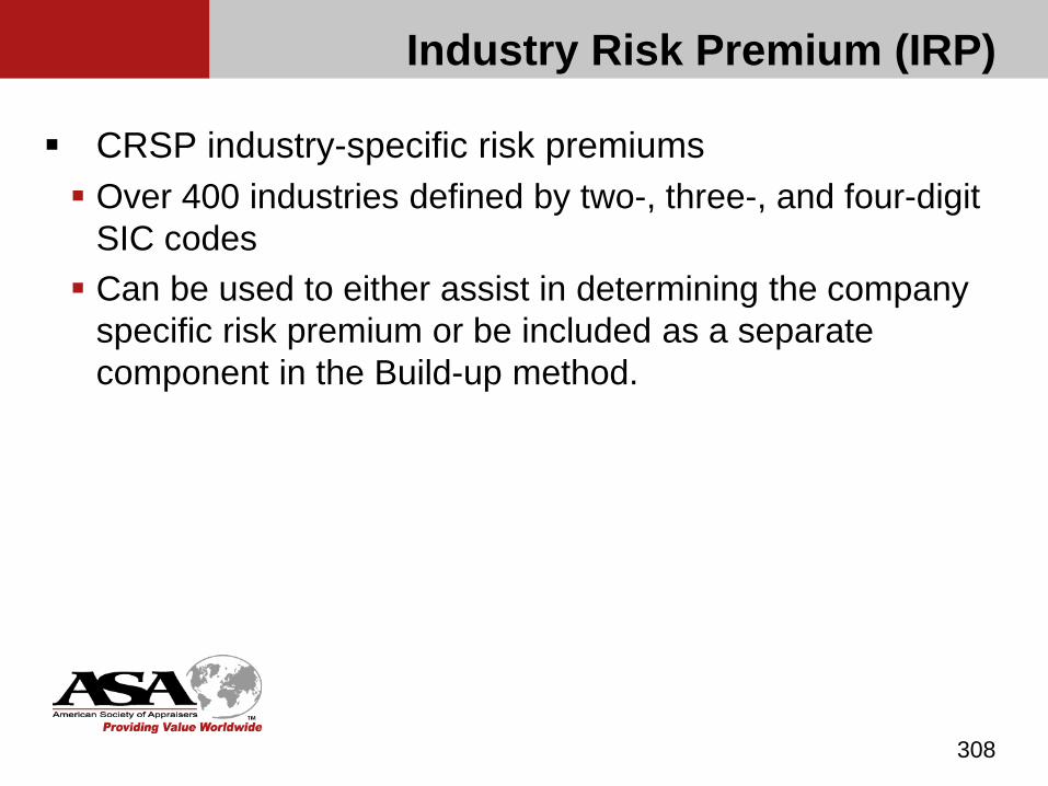
Industry Risk Premium (IRP)
CRSP industry-specific risk premiums Over 400 industries defined by two-, three-, and four-digit
SIC codes Can be used to either assist in determining the company
specific risk premium or be included as a separate component in the Build-up method.
308
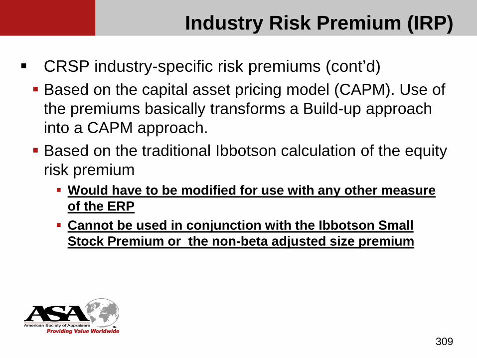
Industry Risk Premium (IRP)
CRSP industry-specific risk premiums (cont’d) Based on the capital asset pricing model (CAPM). Use of
the premiums basically transforms a Build-up approach into a CAPM approach. Based on the traditional Ibbotson calculation of the equity
risk premium Would have to be modified for use with any other measure
of the ERP Cannot be used in conjunction with the Ibbotson Small
Stock Premium or the non-beta adjusted size premium
309

Industry Risk Premium (IRP)
CRSP industry-specific risk premiums (cont’d) Based on full information betas The full information beta (FI beta) is multiplied by the
historical ERP, and then the ERP is subtracted to develop the industry risk premium, as shown below:
IRP = (βFI × ERP) - ERPWhere:
IRP = The industry risk premiumβFI = The full information betaERP = The historical equity risk premium
310
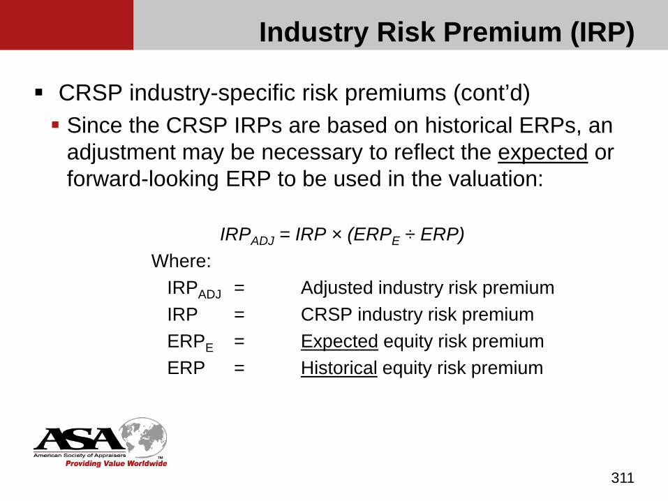
Industry Risk Premium (IRP)
CRSP industry-specific risk premiums (cont’d) Since the CRSP IRPs are based on historical ERPs, an
adjustment may be necessary to reflect the expected or forward-looking ERP to be used in the valuation:
IRPADJ = IRP × (ERPE ÷ ERP)Where:
IRPADJ = Adjusted industry risk premiumIRP = CRSP industry risk premiumERPE = Expected equity risk premiumERP = Historical equity risk premium
311
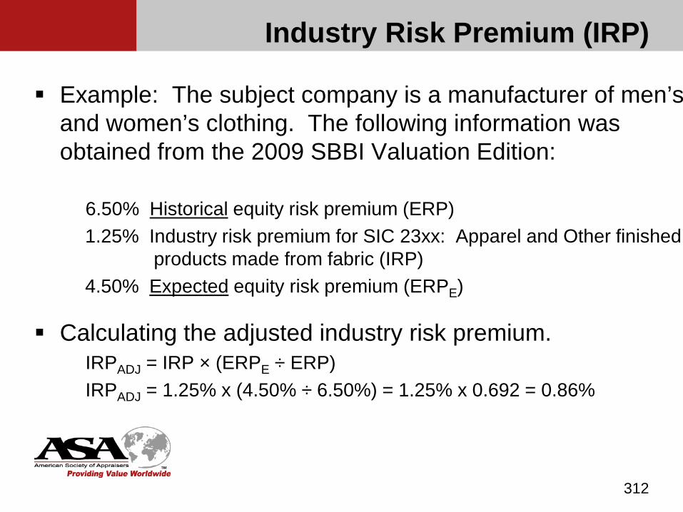
Industry Risk Premium (IRP)
Example: The subject company is a manufacturer of men’s and women’s clothing. The following information was obtained from the 2009 SBBI Valuation Edition:
6.50% Historical equity risk premium (ERP)1.25% Industry risk premium for SIC 23xx: Apparel and Other finished
products made from fabric (IRP)4.50% Expected equity risk premium (ERPE)
Calculating the adjusted industry risk premium.IRPADJ = IRP × (ERPE ÷ ERP)IRPADJ = 1.25% x (4.50% ÷ 6.50%) = 1.25% x 0.692 = 0.86%
312
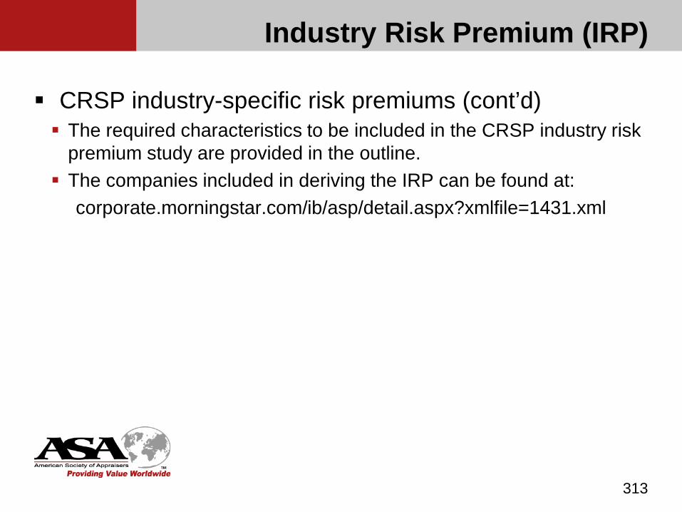
Industry Risk Premium (IRP)
CRSP industry-specific risk premiums (cont’d) The required characteristics to be included in the CRSP industry risk
premium study are provided in the outline. The companies included in deriving the IRP can be found at:
corporate.morningstar.com/ib/asp/detail.aspx?xmlfile=1431.xml
313
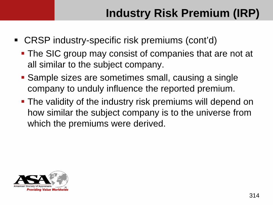
Industry Risk Premium (IRP)
CRSP industry-specific risk premiums (cont’d) The SIC group may consist of companies that are not at
all similar to the subject company. Sample sizes are sometimes small, causing a single
company to unduly influence the reported premium. The validity of the industry risk premiums will depend on
how similar the subject company is to the universe from which the premiums were derived.
314
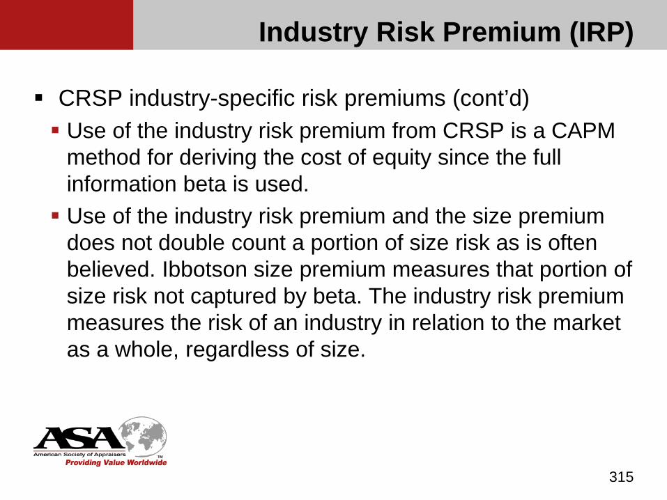
Industry Risk Premium (IRP)
CRSP industry-specific risk premiums (cont’d) Use of the industry risk premium from CRSP is a CAPM
method for deriving the cost of equity since the full information beta is used. Use of the industry risk premium and the size premium
does not double count a portion of size risk as is often believed. Ibbotson size premium measures that portion of size risk not captured by beta. The industry risk premium measures the risk of an industry in relation to the market as a whole, regardless of size.
315

Use of the full information beta as published by D&P converts a traditional beta (which is applied as a multiplier to the equity risk premium in the CAPM) to a discrete amount to be summed with the other components in the build up method. This essentially converts the BUM to a CAPM model, carrying with it all the inherent issues associated with the CAPM (discussed subsequently).
Keep in mind, also, that IRP’s are valid only to the extent that the subject company’s risk characteristics are similar to the weighted average of the companies that make up the SIC code.
316
Industry Risk Premium (IRP)

Industry Risk Premium (IRP)
CRSP industry-specific risk premiums (cont’d) The authors of the D&P Report suggest that the CRSP
industry risk premium (IRPCRSP) data can be used with the D&P Report data designed for use in the Build-up method (exhibits A-1 through A-8). Must be adjusted: IRPADJ = IRP × (ERPE ÷ ERP) May result in double counting of the beta effect.
The authors recommend using the adjusted IRP with the smoothed size premiums obtained from exhibits B-1 to B-8, but assuming a beta of 1.0.
317

Industry Risk Premium (IRP) EXAMPLE: Risk-free rate of 4.5%, traditional ERP of
6.7%, forward-looking ERP estimate of 5.5%, IRP of 2.1%, and an indicated size premium from Ex B-1 to B-8 of 5.1%:
Risk-free rate 4.5%ERP 5.5% (assumes beta = 1.0)Adjusted IRP 1.7% = (5.5% ÷ 6.7%) x 2.1%= Industry CAPM 11.7%Size premium 5.1% (from Ex B-1 to B-8)= ke 16.8%
By assuming a beta of 1.0 and applying the adjusted IRP, the calculation is converted to a CAPM calculation and eliminates any double counting of the beta effect.
318
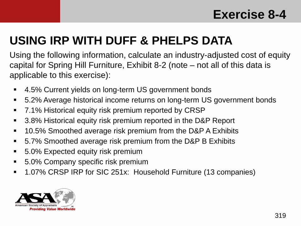
Exercise 8-4
319
USING IRP WITH DUFF & PHELPS DATAUsing the following information, calculate an industry-adjusted cost of equity capital for Spring Hill Furniture, Exhibit 8-2 (note – not all of this data is applicable to this exercise):
4.5% Current yields on long-term US government bonds 5.2% Average historical income returns on long-term US government bonds 7.1% Historical equity risk premium reported by CRSP 3.8% Historical equity risk premium reported in the D&P Report 10.5% Smoothed average risk premium from the D&P A Exhibits 5.7% Smoothed average risk premium from the D&P B Exhibits 5.0% Expected equity risk premium 5.0% Company specific risk premium 1.07% CRSP IRP for SIC 251x: Household Furniture (13 companies)
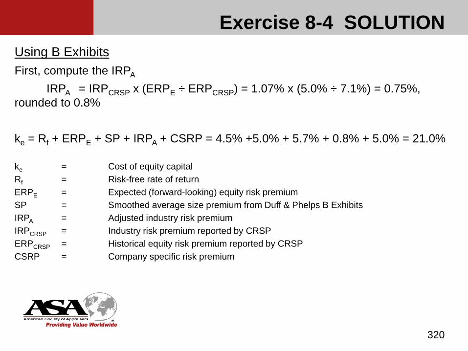
Exercise 8-4 SOLUTION
320
Using B ExhibitsFirst, compute the IRPA
IRPA = IRPCRSP x (ERPE ÷ ERPCRSP) = 1.07% x (5.0% ÷ 7.1%) = 0.75%, rounded to 0.8%
ke = Rf + ERPE + SP + IRPA + CSRP = 4.5% +5.0% + 5.7% + 0.8% + 5.0% = 21.0%
ke = Cost of equity capitalRf = Risk-free rate of returnERPE = Expected (forward-looking) equity risk premiumSP = Smoothed average size premium from Duff & Phelps B ExhibitsIRPA = Adjusted industry risk premiumIRPCRSP = Industry risk premium reported by CRSPERPCRSP = Historical equity risk premium reported by CRSPCSRP = Company specific risk premium
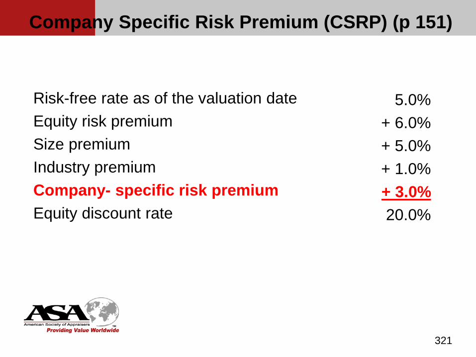
321
Risk-free rate as of the valuation date Equity risk premiumSize premiumIndustry premiumCompany- specific risk premiumEquity discount rate
5.0%+ 6.0%+ 5.0%+ 1.0%+ 3.0%20.0%
Company Specific Risk Premium (CSRP) (p 151)
Company Specific Risk Premium (CSRP)
Little objective data and no quantitative means of establishing the CSRP. While various methods have been developed in an attempt to remove the subjectivity of the CSRP, it remains a matter of judgment and experience.
Important qualitative factors that should be considered (see outline). Business risk Industry Financial risk
322

Company Specific Risk Premium (CSRP)
Some guidance in the BV literature – “The company specific adjustment is usually in the range of a negative 2
percent to a positive 5 percent, but sometimes falls outside that range, and is occasionally as high as positive 10 percent. A 10 percent adjustment could be warranted in extreme circumstances such as a startup company or a financially distressed company.”
“The additional adjustments for size and other risk factors for a small company will range from 3% to 15%. However, adjustments may be significantly greater than 15% for some high-risk companies, or even negative for companies with lower risk than the average small company.”
“Sometimes we see 10 percentage points in the company-specific risk premium, and that, depending on the company and industry, is normally too much. Ten points would push the discount rate close to a venture capital or start-up company rate.”
323
Thus, the guidance offered by the professional literature indicates a range of from -2% for companies with lower risk than the average small, privately held company, to approximately 10% for a company with greater risk than the average small, privately held company.
324
Company Specific Risk Premium (CSRP)
Application of Build Up Discount Rates A discount rate developed using the Build-up
techniques discussed in this chapter should be applied to a stream of equity net cash flow from a C corporation. This correctly matches the character of the returns used
to develop the ERP component of the discount rate. Issues associated with using Build-up equity discount
rates (and rates based upon CAPM) to value S corporations are presented in BV204.
325
A discount rate developed using the Build-up method does not have a “minority” or “control” character. The fundamental business risk does not change with the
ownership level. Other risks do change with the ownership level, including
the ability to readily sell the interest, influence operations, and realize a return on the investment, but these risks are captured in the discounts and premiums.
326
Application of Build Up Discount Rates
Theoretically, a discount rate applicable to equity net cash flow could be adjusted to apply to a different income stream. Introduces other inconsistencies in the calculation of
value. Grossing up an after-tax discount rate to a pre-tax rate
and applying it to pre-tax cash flow will not yield the same result as using after-tax cash flow and an after-tax discount rate due to timing of cash flows versus expenses of capital expenditures.
327
Application of Build Up Discount Rates
Start-up & Early Stage Companies (p 153) A business enterprise generally follows a lifecycle that
includes three or four stages Start-up Growth Maturity Decline
328
Start-up and Early Stage Companies The premise of the cost of equity is the same for
companies in all four stages. That is, investors are risk averse and will require additional return for accepting more risk.
The studies that analysts frequently use to estimate risk premiums are based on publicly-traded operating companies generally in the growth, maturity, or decline stages.
329
Start-up and Early Stage Companies However, the analyst frequently must value interests in
start-up and early stage companies. No history, in need of capital, and undeveloped or
unproven products/services = additional risk Everything else being equal, companies in the start-up
stage will have higher costs of equity than those in the other three stages.
330

Start-up and Early Stage Companies The AICPA Practice Aid Valuation of Privately-Held-
Company Equity Securities as Compensation Identifies six stages of business enterprise
development
331
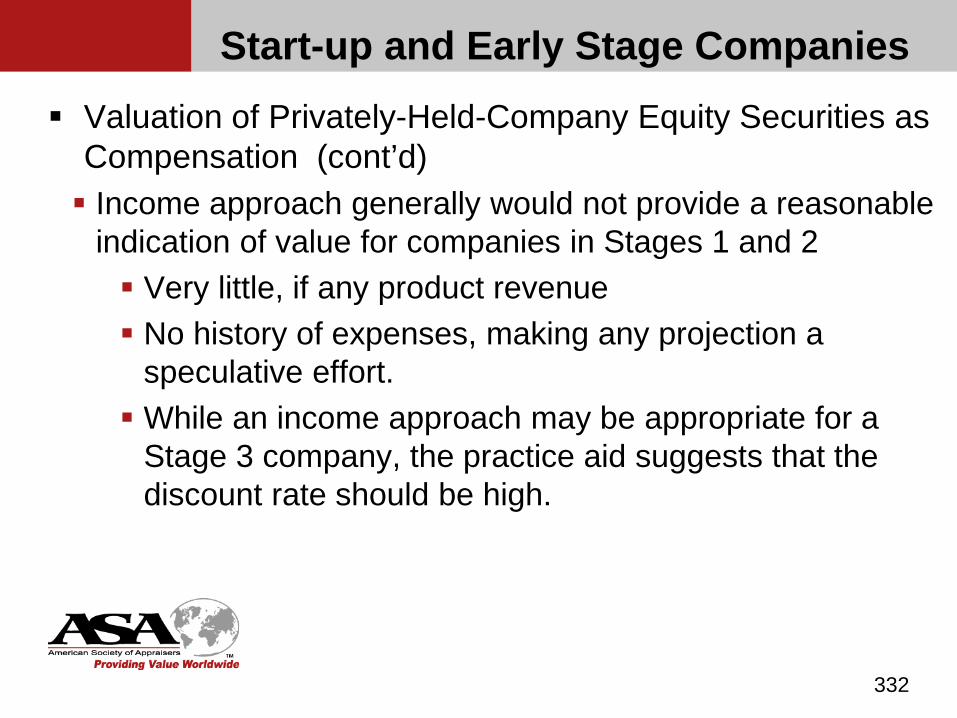
Start-up and Early Stage Companies Valuation of Privately-Held-Company Equity Securities as
Compensation (cont’d) Income approach generally would not provide a reasonable
indication of value for companies in Stages 1 and 2 Very little, if any product revenue No history of expenses, making any projection a
speculative effort. While an income approach may be appropriate for a
Stage 3 company, the practice aid suggests that the discount rate should be high.
332
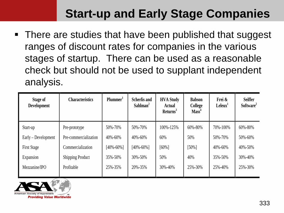
Start-up and Early Stage Companies There are studies that have been published that suggest
ranges of discount rates for companies in the various stages of startup. There can be used as a reasonable check but should not be used to supplant independent analysis.
333
Stage of Development
Characteristics Plummer1 Scherlis and Sahlman2
HVA Study Actual
Returns3
Babson College Mass4
Frei & Leleux1
Seiffer Software2
Start-up
Early – Development
First Stage
Expansion
Mezzanine/IPO
Pre-prototype
Pre-commercialization
Commercialization
Shipping Product
Profitable
50%-70%
40%-60%
[40%-60%]
35%-50%
25%-35%
50%-70%
40%-60%
[40%-60%]
30%-50%
20%-35%
100%-125%
60%
[60%]
50%
30%-40%
60%-80%
50%
[50%]
40%
25%-30%
70%-100%
50%-70%
40%-60%
35%-50%
25%-40%
60%-80%
50%-60%
40%-50%
30%-40%
25%-30%
Chapter 9
Capital Asset Pricing Model
334

History and Derivation (page 165)
History Originally developed in 1964. Developed in the context of portfolio theory, as a means
of measuring the risk that an individual stock contributes to a well-diversified portfolio. Based on “efficient market” theory, which suggests that
security prices in public markets will not depart for any length of time from their justified economic values. The original model was not intended to derive the cost of
equity for an individual stock. It has been adapted for this purpose through the modifications explained here.
335
History and Derivation
Derivation of CAPM Diversifiable or unsystematic risk – The risk of random
negative events particular to a subject company such as labor strikes, failed product launches, lawsuits, departures of key personnel, etc. Diversifiable in that by adding other investments to the portfolio,
this risk can be diversified away
Unsystematic in that it follows no pattern in relationship to the market in general due to factors unique to the specific company
336
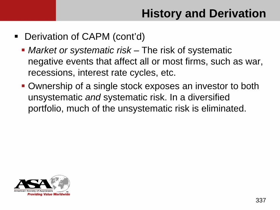
History and Derivation
Derivation of CAPM (cont’d) Market or systematic risk – The risk of systematic
negative events that affect all or most firms, such as war, recessions, interest rate cycles, etc. Ownership of a single stock exposes an investor to both
unsystematic and systematic risk. In a diversified portfolio, much of the unsystematic risk is eliminated.
337
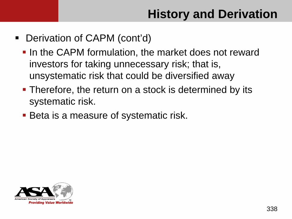
History and Derivation
Derivation of CAPM (cont’d) In the CAPM formulation, the market does not reward
investors for taking unnecessary risk; that is, unsystematic risk that could be diversified away Therefore, the return on a stock is determined by its
systematic risk. Beta is a measure of systematic risk.
338
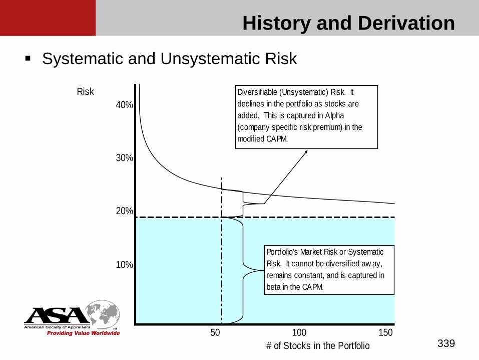
History and Derivation Systematic and Unsystematic Risk
339
Risk40%
30%
20%
10%
50 100 150# of Stocks in the Portfolio
Portfolio's Market Risk or Systematic Risk. It cannot be diversif ied aw ay, remains constant, and is captured in beta in the CAPM.
Diversif iable (Unsystematic) Risk. It declines in the portfolio as stocks are added. This is captured in Alpha (company specif ic risk premium) in the modif ied CAPM.
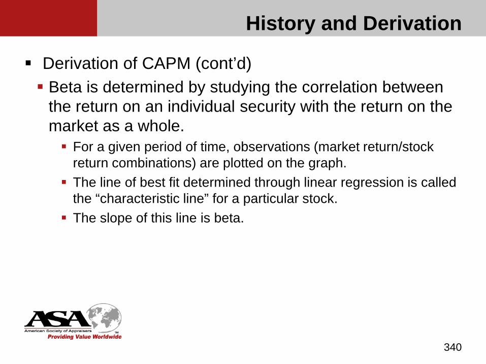
History and Derivation
Derivation of CAPM (cont’d) Beta is determined by studying the correlation between
the return on an individual security with the return on the market as a whole. For a given period of time, observations (market return/stock
return combinations) are plotted on the graph. The line of best fit determined through linear regression is called
the “characteristic line” for a particular stock. The slope of this line is beta.
340

History and DerivationYear 1 Year 2 Year 1 Year 2
Stock X return –25% 40% Market return –10% 20%
341
History and Derivation
Derivation of CAPM The security market line depicts the relationship
between risk and return that is derived from CAPM. It is the line on the graph that connects the return on a
portfolio comprised 100% of the risk-free security and a portfolio that is comprised of the general equity market and fully diversified. No security whose risk and return place it above or below
the security market line is desirable. So, the market will re-price the security until it achieves a relationship of risk and return that is consistent with the security market line.
342

Security Market Line
343
ReturnsRe = 17%
Rm = 11%
Rf = 5%
0 2.0Risk
Measured by beta
1.0
Market Equity Risk Premium (ERP) = 6%
SML: Ke = Rf + β(ERP) = 5% + β(6%)
Portfolio A: 100% in risk-free investments
Portfolio B: 100% in the equity market;
sufficiently large portfolio
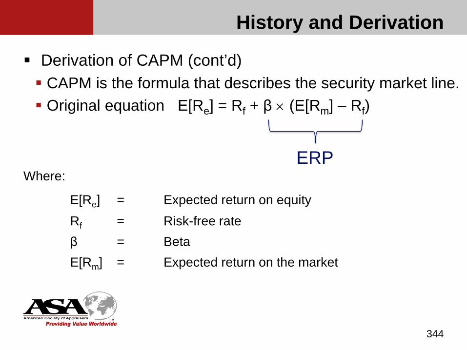
History and Derivation
Derivation of CAPM (cont’d) CAPM is the formula that describes the security market line. Original equation E[Re] = Rf + β × (E[Rm] – Rf)
Where:
E[Re] = Expected return on equityRf = Risk-free rate β = BetaE[Rm] = Expected return on the market
344
ERP
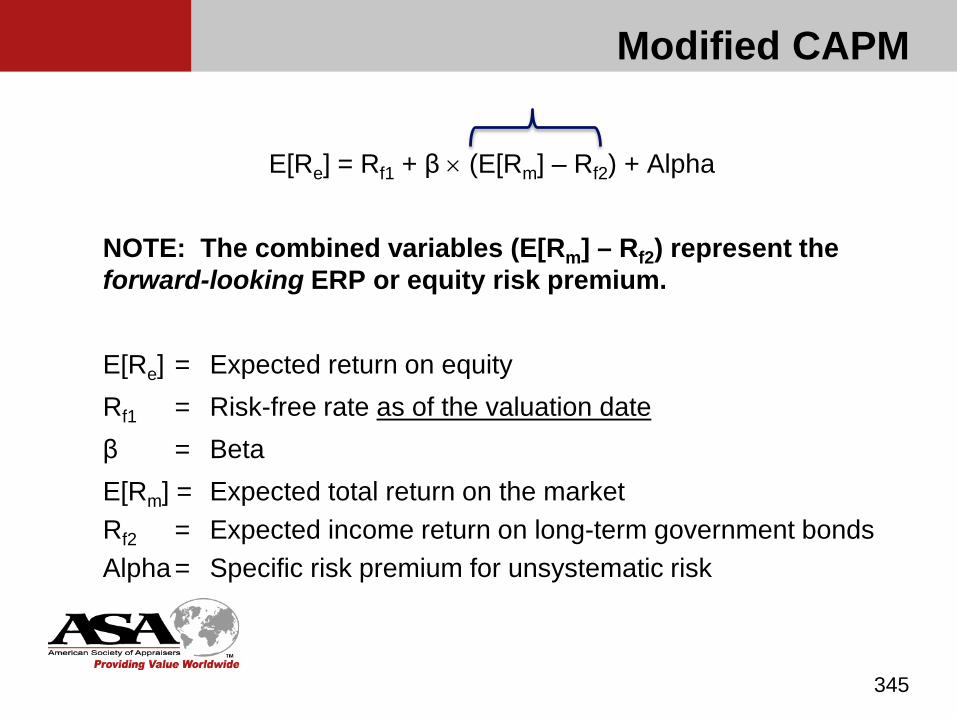
Modified CAPM
E[Re] = Rf1 + β × (E[Rm] – Rf2) + Alpha
NOTE: The combined variables (E[Rm] – Rf2) represent the forward-looking ERP or equity risk premium.
E[Re] = Expected return on equityRf1 = Risk-free rate as of the valuation dateβ = BetaE[Rm] = Expected total return on the marketRf2 = Expected income return on long-term government bondsAlpha= Specific risk premium for unsystematic risk
345
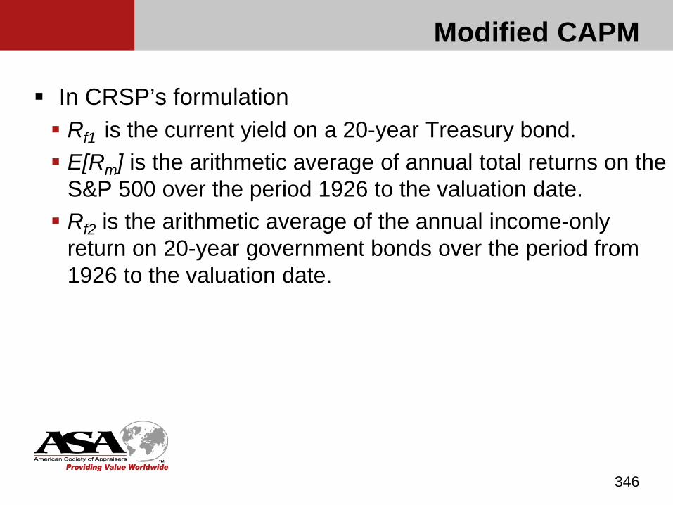
Modified CAPM
In CRSP’s formulation Rf1 is the current yield on a 20-year Treasury bond. E[Rm] is the arithmetic average of annual total returns on the
S&P 500 over the period 1926 to the valuation date. Rf2 is the arithmetic average of the annual income-only
return on 20-year government bonds over the period from 1926 to the valuation date.
346

Modified CAPM
Size premiums in CAPM The original CAPM accounts for some, but not all, of the risk
associated with size. In CRSP, betas for each of the 10 portfolios of stocks are
calculated by regressing the monthly total returns of the portfolio in excess of the 30-day U.S. Treasury bill versus the S&P 500 total returns in excess of the U.S. Treasury bill. Therefore, the beta of each portfolio should contain some
risk associated with size.
347

Modified CAPM
Size premiums in CAPM (cont’d) The actual realized returns in each size decile are generally
greater than the estimated return using the beta and the ERP as calculated above. This difference between this calculated return and actual realized return is referred to in CRSP as the beta-adjusted size premium. Both the CRSP beta-adjusted size premiums and the Duff &
Phelps smoothed size premiums from the B Exhibits may be used with the modified CAPM.
348

Modified CAPM
Alpha Measurement of alpha in the modified CAPM is subjective
and is generally considered to include a size premium and a premium for subject company risk. Any industry risk premium (or discount) is thought to be subsumed in beta (depending on the source(s) used to derive beta).
349

Key Assumptions of CAPM (page 169)
Investors are risk averse. Generally an acceptable assumption.
Rational investors seek to hold efficient portfolios; that is, portfolios that are well diversified. Interests in privately-held companies are generally not held
in large, well diversified portfolios.
350
Key Assumptions of CAPM
All investors have identical expectations about such variables as expected rates of return and how capitalization factors are generated. May not be the case.
There are no investment-related taxes or transaction costs. Not a valid assumption.
351
Key Assumptions of CAPM
Relative price volatility (beta) is a modifier of equity market risk and required return. Beta volatility is not a good indicator of return; beta volatility
may not be a good measure of risk.
The rate received from lending money is the same as the cost of borrowing money. Not a valid assumption.
The market has perfect divisibility and liquidity.
352
Key Assumptions of CAPM
Other problems with the Assumptions The model assumes that all investors have complete or
exactly equivalent knowledge and the market is rational. Investors in closely held securities generally have a longer
holding period than investors in public companies. The equation was meant to be conceptual, not a formula for
calculating rates of return for individual securities.
353
Derivation of Betas (page 170)
Beta is a relationship obtained from regressing an individual stock's total return (dividends and capital appreciation) against a market return such as the S&P 500. β = 1.0: total return for the subject security moves in tandem
with the total return of the market. β > 1.0: total return for the subject security moves in the
same direction as the market but with greater magnitude.
354

Derivation of Betas
Beta (cont’d) β < 1.0: total return for the subject security moves in the
same direction as the market but with less magnitude. β < 0.0: total return for the subject security moves in the
opposite direction from the total return on the market.
355

Use of Betas
Betas are unavailable for private companies. Typical practice is to develop an estimate of beta from
guideline public companies. Used this way, beta assumes the function of an industry
risk component. In the CAPM formula, beta is multiplied by the equity risk
premium (ERP = Rm – Rf1), not the sum of the ERP and the size risk premium.
356
Use of Betas (page 171)
Small company risks must be added later. Un-levering and Re-levering Betas Published betas for publicly traded stock reflect the capital structure and
financial leverage of those companies. Guideline betas may be un-levered to remove the effect of financial
leverage leaving the effect of operating risk only, then re-lever to reflect the leverage of the subject company
Two methods Hamada Formula Harris-Pringle Formula
357
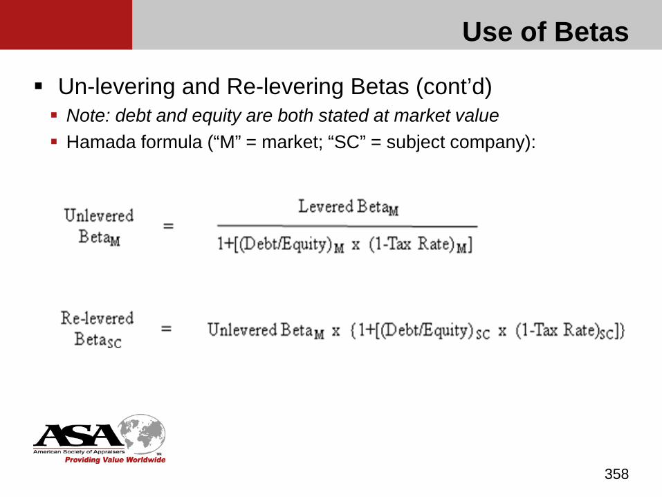
Use of Betas
Un-levering and Re-levering Betas (cont’d) Note: debt and equity are both stated at market value Hamada formula (“M” = market; “SC” = subject company):
358
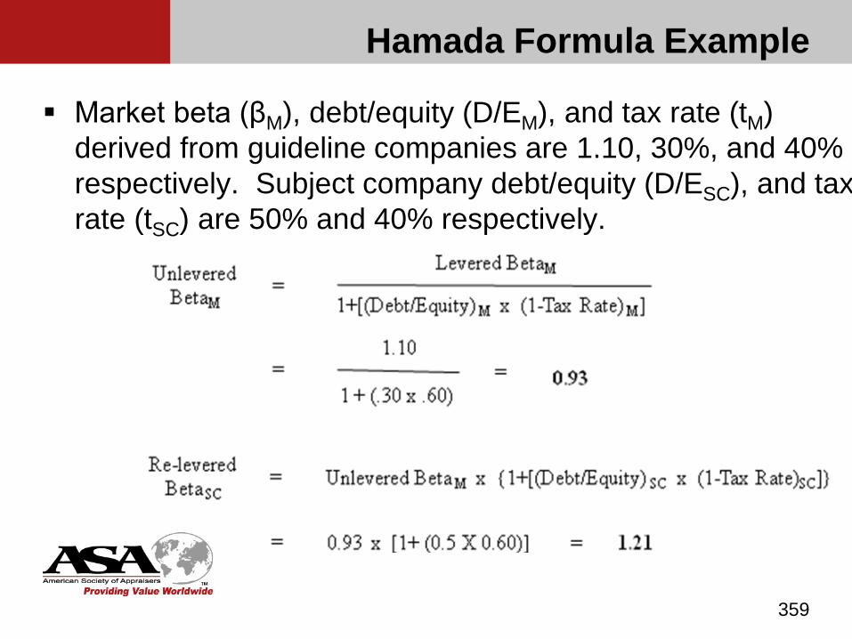
Hamada Formula Example
Market beta (βM), debt/equity (D/EM), and tax rate (tM) derived from guideline companies are 1.10, 30%, and 40% respectively. Subject company debt/equity (D/ESC), and tax rate (tSC) are 50% and 40% respectively.
359
Use of Betas
Un-levering and Re-levering Betas (cont’d) Hamada formula (cont’d) The Hamada Formula is based on an assumption of
constant debt (dollars). It is problematic when used under the assumption of constant relative debt to equity.
360
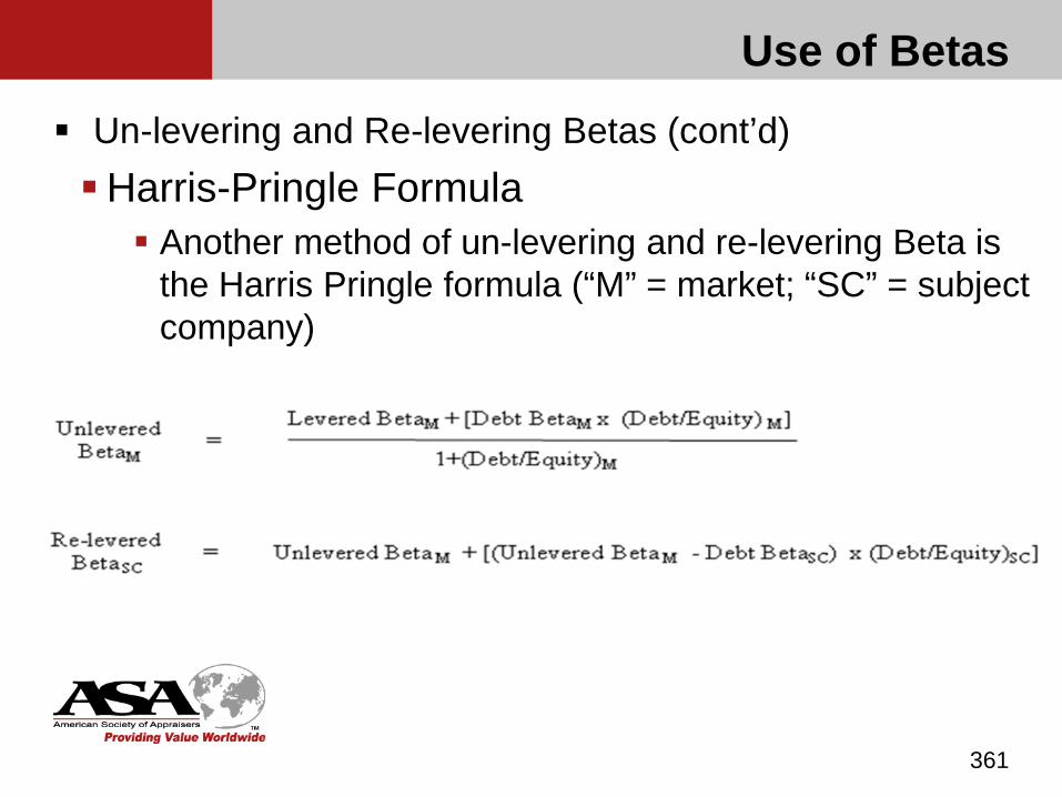
Use of Betas
Un-levering and Re-levering Betas (cont’d)Harris-Pringle Formula Another method of un-levering and re-levering Beta is
the Harris Pringle formula (“M” = market; “SC” = subject company)
361
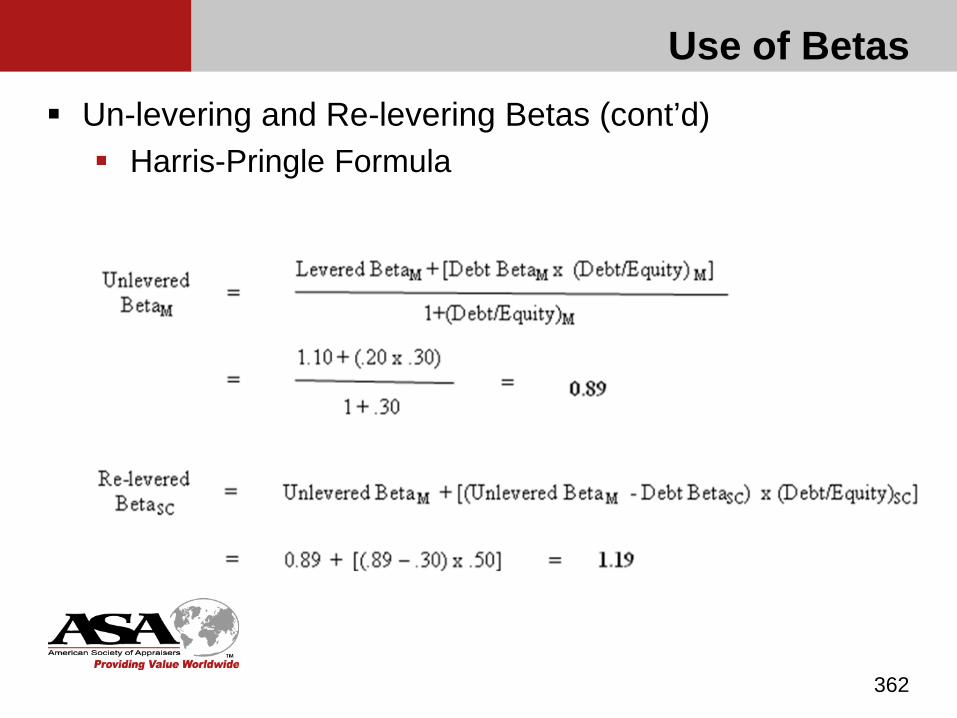
Use of Betas Un-levering and Re-levering Betas (cont’d) Harris-Pringle Formula
362
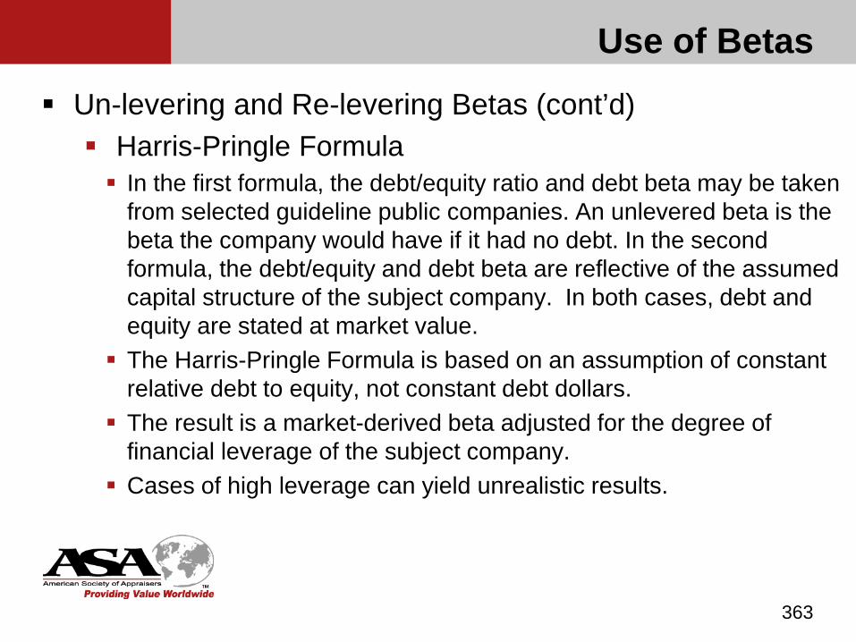
Use of Betas Un-levering and Re-levering Betas (cont’d) Harris-Pringle Formula In the first formula, the debt/equity ratio and debt beta may be taken
from selected guideline public companies. An unlevered beta is the beta the company would have if it had no debt. In the second formula, the debt/equity and debt beta are reflective of the assumed capital structure of the subject company. In both cases, debt and equity are stated at market value.
The Harris-Pringle Formula is based on an assumption of constant relative debt to equity, not constant debt dollars.
The result is a market-derived beta adjusted for the degree of financial leverage of the subject company.
Cases of high leverage can yield unrealistic results.
363

Exercise 9-1
364
RE-LEVERING BETASUsing the Hamada formula and the Harris-Pringle Formula, derive the re-levered beta under the following assumptions:
Levered guideline beta = 1.22 Guideline debt to invested capital is 35% Guideline tax rate is 40% Company market value of invested capital is $75 million Company book value of invested capital is $33 million Company market and book value of debt is $10 million Company tax rate is 40% Market debt beta is 0.15 Company debt beta 0.18
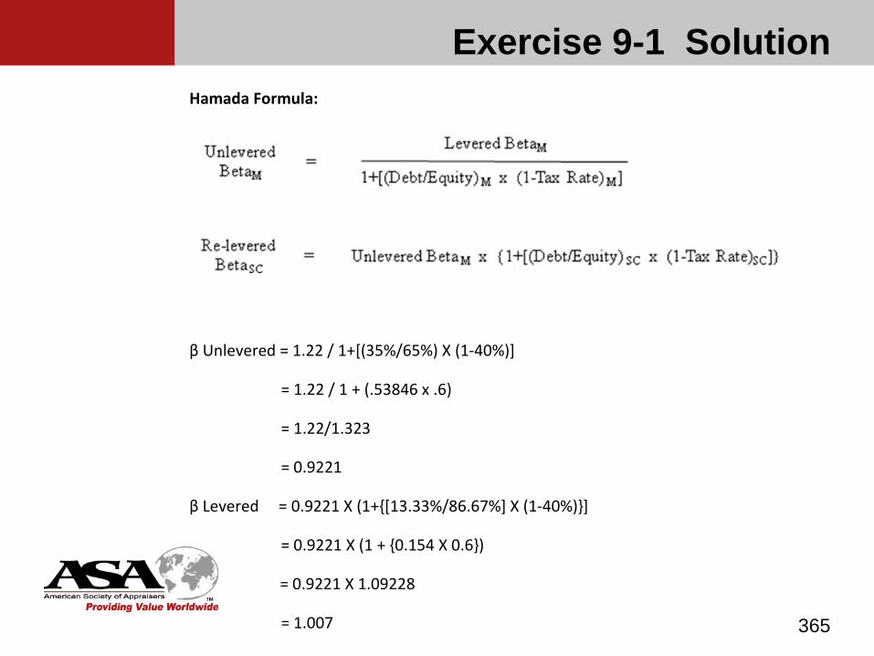
Exercise 9-1 Solution
365
Hamada Formula:
β Unlevered = 1.22 / 1+[(35%/65%) X (1-40%)]
= 1.22 / 1 + (.53846 x .6)
= 1.22/1.323
= 0.9221
β Levered = 0.9221 X (1+{[13.33%/86.67%] X (1-40%)}]
= 0.9221 X (1 + {0.154 X 0.6})
= 0.9221 X 1.09228
= 1.007
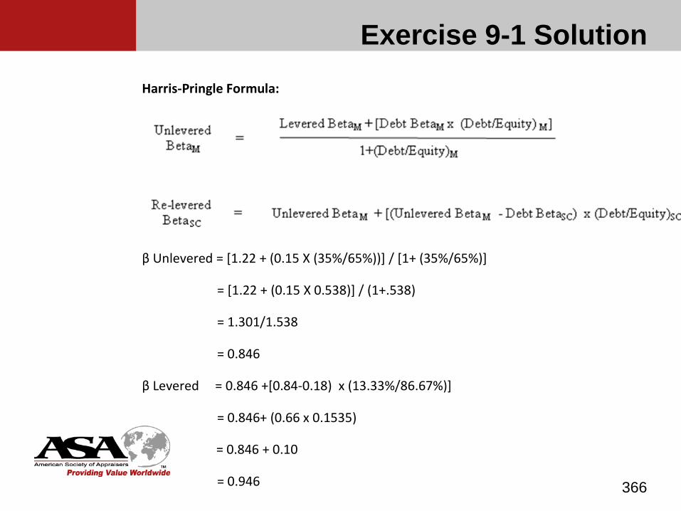
Exercise 9-1 Solution
366
Harris-Pringle Formula:
β Unlevered = [1.22 + (0.15 X (35%/65%))] / [1+ (35%/65%)]
= [1.22 + (0.15 X 0.538)] / (1+.538)
= 1.301/1.538
= 0.846
β Levered = 0.846 +[0.84-0.18) x (13.33%/86.67%)]
= 0.846+ (0.66 x 0.1535)
= 0.846 + 0.10
= 0.946

Sources of Betas (page 175)
Betas are not stable over time, nor are they calculated in the same way by the different services that report betas.
Within any assignment, betas should be obtained from the same source to ensure consistency in how they are derived
367
Sources of Betas
Common sources Standard & Poor’s Sixty monthly returns are used in the calculation (five
years) Sharp or sudden changes are not “smoothed.” Stock performance is regressed against the S&P 500.
Value Line Weekly returns are used in the calculation. Sharp or sudden changes are not “smoothed.” Stock performance is regressed against the NYSE.
368
Sources of Betas
Common sources (cont’d) Media General Financial Services’ IndustriScope Thirty-six month-end returns used in the calculations
(three years) Regressed against the S&P 500
Morningstar’s (formerly Ibbotson’s) Beta Book Yahoo Finance, Hoovers and other Internet source A history of industry betas can be found at New York
University’s Stern School of Management
369
Challenges to the CAPM
It is important to remember that CAPM was not originally intended for use in business appraisal. An appraiser who uses this methodology must have a thorough understanding of the model, its theoretical constraints, and weaknesses created by its use in the appraisal process.
370
Application of CAPM Discount Rates
Since the ERP component is the same between CAPM and Build-up discount rates, the reasoning about the nature of the resulting discount rate is the same.
A discount rate developed using CAPM should be applied to a stream of equity net cash flow from a C corporation.
371
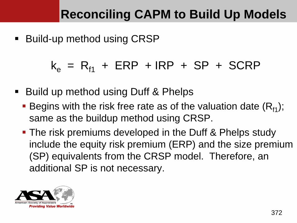
Reconciling CAPM to Build Up Models
Build-up method using CRSP
ke = Rf1 + ERP + IRP + SP + SCRP
Build up method using Duff & Phelps Begins with the risk free rate as of the valuation date (Rf1);
same as the buildup method using CRSP. The risk premiums developed in the Duff & Phelps study
include the equity risk premium (ERP) and the size premium (SP) equivalents from the CRSP model. Therefore, an additional SP is not necessary.
372

Reconciling CAPM to Build Up Models
Build up method using Duff & Phelps (cont’d) The underlying data used to develop CRSP is different than
that used to develop the Duff & Phelps study in terms of how far back each study reaches and in terms of the estimated ERP resulting from each study. Some analysts suggest that the industry risk premiums
(IRP) reported in CRSP should not be used in a build up method based on the Duff & Phelps. Others suggest that the IRP can be adjusted for the
difference in the studies’ ERPs and used with the Duff & Phelps data.
373

Reconciling CAPM to Build Up Models
Build up method using Duff & Phelps (cont’d) A particular company’s cost of equity should not vary due simply to
different sources of data or methodologies used to estimate that rate.
As a practical matter, of course, they do differ, depending on the selection of: The beginning point for computing the equity risk premium (1926? 1963? Other?) The measurement of Beta (Monthly returns? Weekly returns?) Which market the returns are regressed against (S&P? NYSE?) The use of ten deciles (CRSP) or twenty five portfolios (D&P) How the size premium is measured (CRSP or “baked in” to the D&P equations)
374

Reconciling CAPM to Build Up Models
Modified CAPMke = Rf1 + β(ERP) + Alpha
Begins with Rf1 same as the buildup method using CRSP or Duff & Phelps.
The ERP in the modified CAPM model is the same as that used in CRSP.
Depending on the source(s) of the beta (β) used, a component of the industry risk premium (IRP) and the size premium (SP) may be accounted for by using beta.
375
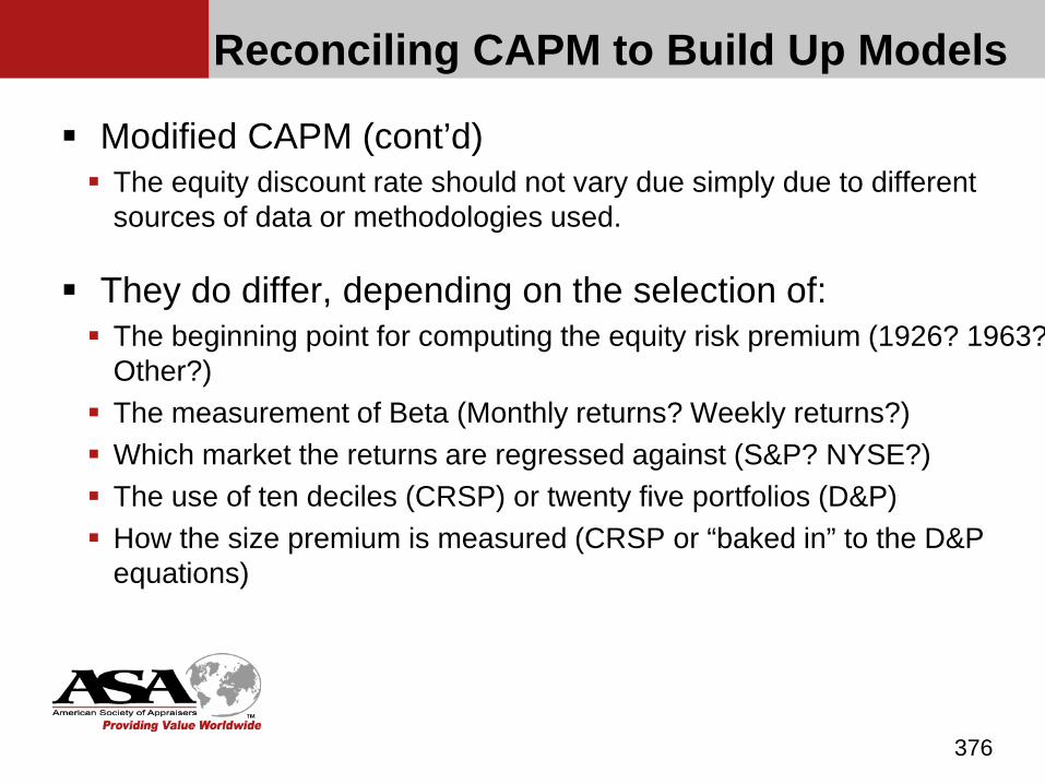
Reconciling CAPM to Build Up Models
Modified CAPM (cont’d) The equity discount rate should not vary due simply due to different
sources of data or methodologies used.
They do differ, depending on the selection of: The beginning point for computing the equity risk premium (1926? 1963?
Other?) The measurement of Beta (Monthly returns? Weekly returns?) Which market the returns are regressed against (S&P? NYSE?) The use of ten deciles (CRSP) or twenty five portfolios (D&P) How the size premium is measured (CRSP or “baked in” to the D&P
equations)
376
Exercise 9-2
377
APPLYING THE CAPM AND BUILD-UP MODELSUsing the data in Exhibit 9-1 at the end of the chapter and the D&P data in Appendix 8-1, develop an estimate for the cost of equity for Reconcile Corp. using the Build-up Method (both CRSP and Duff & Phelps) and CAPM. Use the regression equations of the B Exhibits for the Duff & Phelps Buildup
Method.
Re-lever beta using Harris-Pringle. Refer to Appendix 8-1 for the Duff & Phelps exhibits. Assume a Company Specific Risk Premium (CSRP) of zero. To the extent that the estimates under each method vary, record possible
explanations for the differences and/or what might reconcile them.
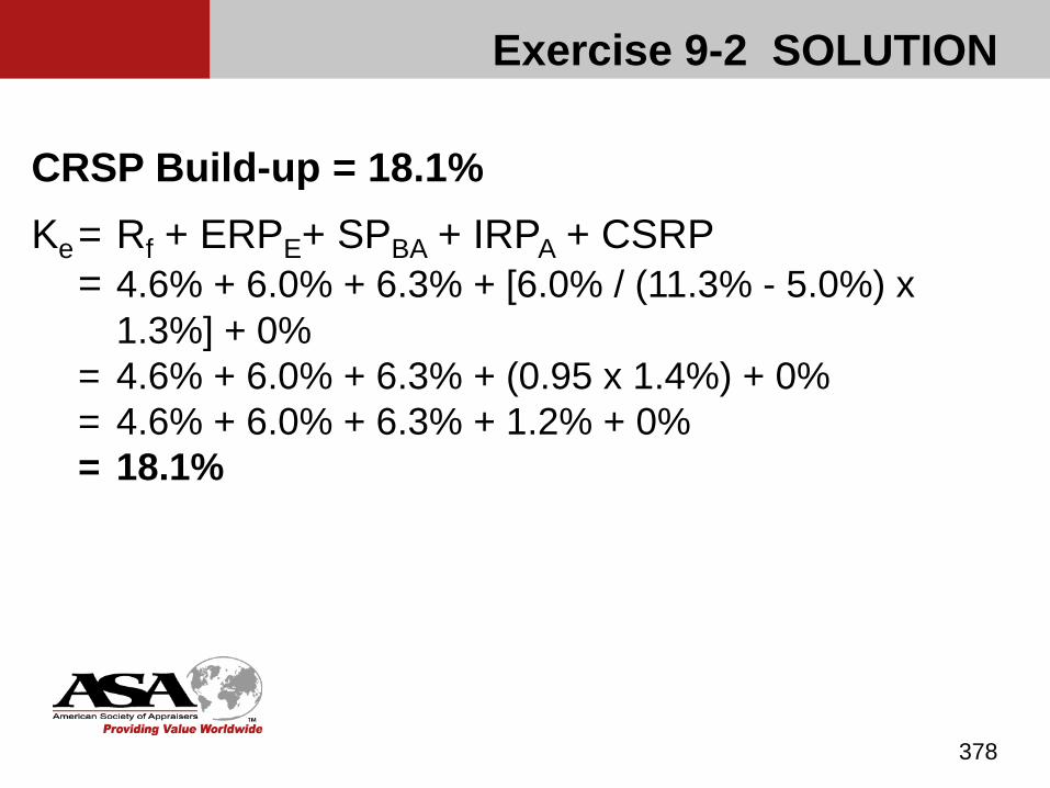
378
CRSP Build-up = 18.1%Ke= Rf + ERPE+ SPBA + IRPA + CSRP
= 4.6% + 6.0% + 6.3% + [6.0% / (11.3% - 5.0%) x 1.3%] + 0%
= 4.6% + 6.0% + 6.3% + (0.95 x 1.4%) + 0%= 4.6% + 6.0% + 6.3% + 1.2% + 0%= 18.1%
Exercise 9-2 SOLUTION
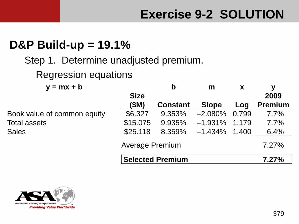
Exercise 9-2 SOLUTION
379
D&P Build-up = 19.1%Step 1. Determine unadjusted premium.
Regression equationsy = mx + b b m x y
Size($M) Constant Slope Log
2009 Premium
Book value of common equity $6.327 9.353% −2.080% 0.799 7.7%Total assets $15.075 9.935% −1.931% 1.179 7.7%Sales $25.118 8.359% −1.434% 1.400 6.4%
Average Premium 7.27%
Selected Premium 7.27%
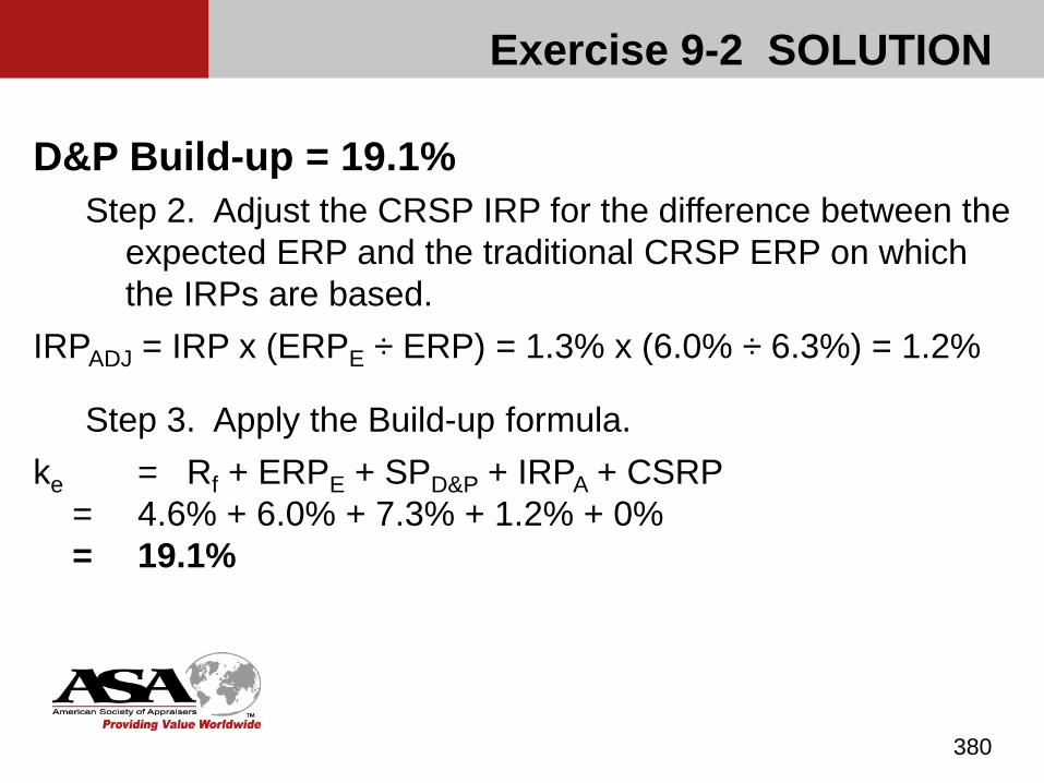
Exercise 9-2 SOLUTION
380
D&P Build-up = 19.1%Step 2. Adjust the CRSP IRP for the difference between the
expected ERP and the traditional CRSP ERP on which the IRPs are based.
IRPADJ = IRP x (ERPE ÷ ERP) = 1.3% x (6.0% ÷ 6.3%) = 1.2%
Step 3. Apply the Build-up formula.ke = Rf + ERPE + SPD&P + IRPA + CSRP
= 4.6% + 6.0% + 7.3% + 1.2% + 0%= 19.1%
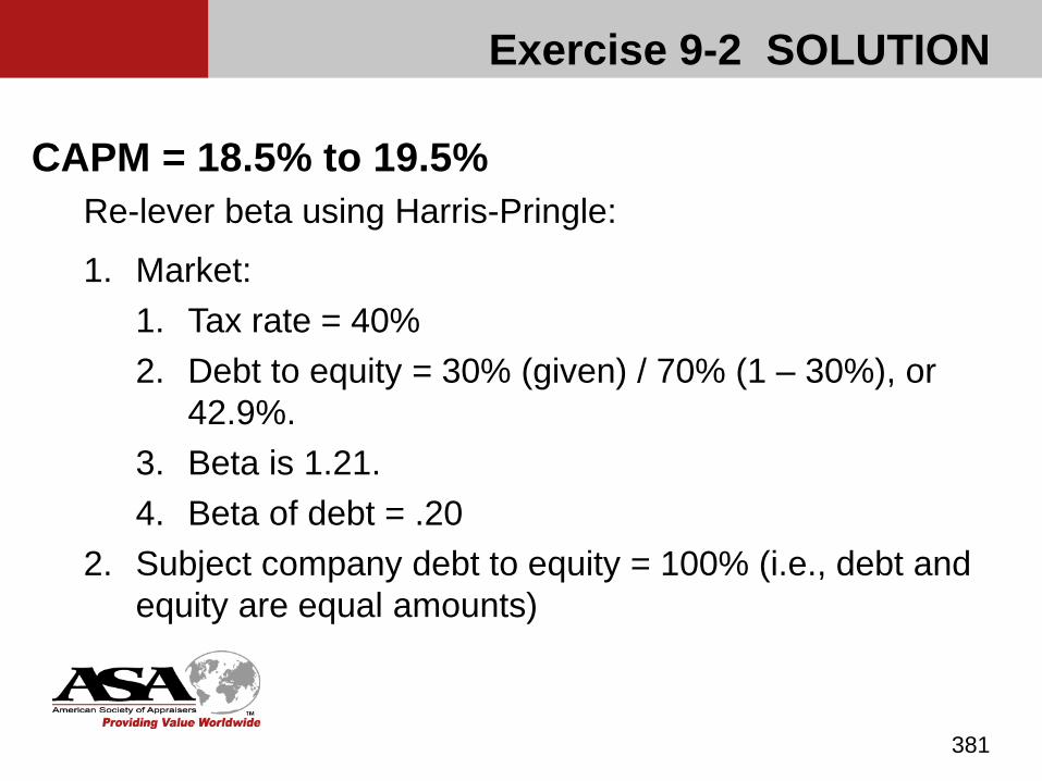
Exercise 9-2 SOLUTION
381
CAPM = 18.5% to 19.5%Re-lever beta using Harris-Pringle:
1. Market:1. Tax rate = 40% 2. Debt to equity = 30% (given) / 70% (1 – 30%), or
42.9%. 3. Beta is 1.21.4. Beta of debt = .20
2. Subject company debt to equity = 100% (i.e., debt and equity are equal amounts)
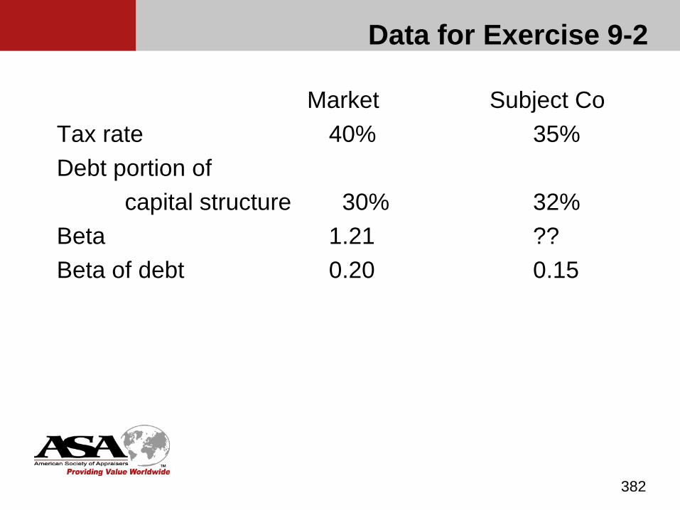
Data for Exercise 9-2
Market Subject CoTax rate 40% 35%Debt portion of
capital structure 30% 32%Beta 1.21 ??Beta of debt 0.20 0.15
382

EXERCISE 9-2 SOLUTION
383
Harris-Pringle Formula:
β Unlevered = [1.21 + (0.20 X (30%/70%))] / [1+ (30%/70%)]
= [1.21 + (0.20 X 0.429)] / (1+.429)
= 1.296/1.429
= 0.907
β Levered = 0.907 + [0.907 - 0.15) x (32%/68%)]
= 0.907 + (0.757 x 0.471)
= 0.907 + 0.36
= 1.267
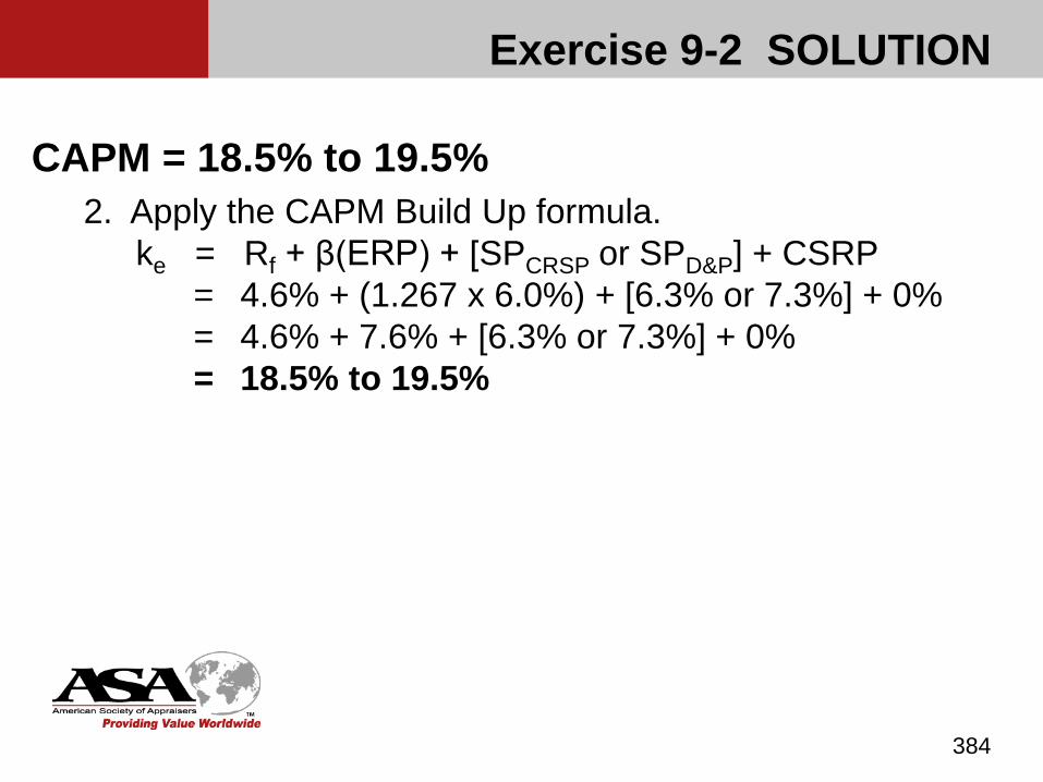
Exercise 9-2 SOLUTION
384
CAPM = 18.5% to 19.5%2. Apply the CAPM Build Up formula.
ke = Rf + β(ERP) + [SPCRSP or SPD&P] + CSRP = 4.6% + (1.267 x 6.0%) + [6.3% or 7.3%] + 0%= 4.6% + 7.6% + [6.3% or 7.3%] + 0%= 18.5% to 19.5%
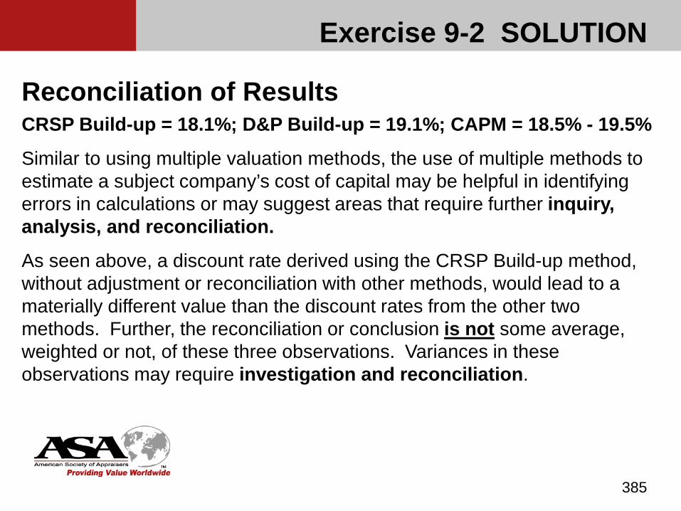
Exercise 9-2 SOLUTION
385
Reconciliation of ResultsCRSP Build-up = 18.1%; D&P Build-up = 19.1%; CAPM = 18.5% - 19.5%
Similar to using multiple valuation methods, the use of multiple methods to estimate a subject company’s cost of capital may be helpful in identifying errors in calculations or may suggest areas that require further inquiry, analysis, and reconciliation.
As seen above, a discount rate derived using the CRSP Build-up method, without adjustment or reconciliation with other methods, would lead to a materially different value than the discount rates from the other two methods. Further, the reconciliation or conclusion is not some average, weighted or not, of these three observations. Variances in these observations may require investigation and reconciliation.

Exercise 9-2 SOLUTION
386
Reconciliation of ResultsCRSP Build-up = 18.1%; D&P Build-up = 19.1%; CAPM = 18.5% - 19.5%
The CRSP and Duff & Phelps indications account for industry risk and size risk, but do not account for additional risk, if any, from greater use of leverage (i.e., we did not re-lever the risk premium). Which model, in this case, presents a more credible representation of the additional risk for the size of Reconcile Corporation?

Exercise 9-2 SOLUTION
387
Reconciliation of ResultsCRSP Build-up = 18.1%; D&P Build-up = 19.1%; CAPM = 18.5% - 19.5%
The CAPM indication also accounts for industry risk and size risk. The unlevered beta of 0.96 implies an industry risk premium of -.24% (i.e., {0.96 - 1.00} x 6% ERP). The CAPM size premium is derived from either CRSP or Duff & Phelps. The CAPM indication also accounts for the greater leverage employed by Reconcile. The incremental beta, when re-levered (i.e., 1.26 versus 0.96) suggests an additional 1.8% risk premium (i.e., {1.26 – 0.96} x 6% ERP) in the CAPM model for Reconcile for the additional leverage. Neither of the buildup models captured that incremental risk. .

Exercise 9-2 SOLUTION
388
Reconciliation of ResultsCRSP Build-up = 18.1%; D&P Build-up = 19.1%; CAPM = 18.5% - 19.5%
On a theoretical basis, the three models would produce the same estimate of cost of capital. The reconciliation ultimately rests in alpha, or the unsystematic risk of a subject company that has not been adjusted for in the other components of the cost-of-capital equations.
Chapter 10
Weighted Average Cost of Capital
389
Definition and Formula (page 184)
The weighted average cost of capital (WACC) is A cost of capital (“discount rate”) determined by a
weighted average, at market value, of the cost of all financing sources in the business enterprise’s capital structure. (BVS Definitions) A blended rate that reflects the required rates of return to
both debt and equity. It also reflects the capital structure and the tax rate. WACC is a discount rate (a rate of return), not a
capitalization rate.
390

Definition and Formula
When correctly applied to invested capital net cash flow, a WACC discount rate results in the market value of invested capital (MVIC). Invested capital is The sum of the debt and equity in an enterprise on a
long-term basis (BVS Definitions). The sum of the market value of debt and equity. The sum of net working capital plus fixed assets plus
the market value of intangible assets.
391
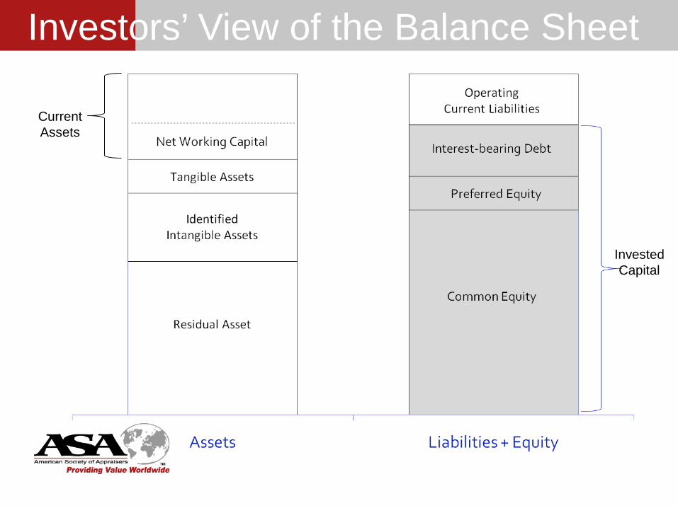
CurrentAssets
InvestedCapital
Investors’ View of the Balance Sheet
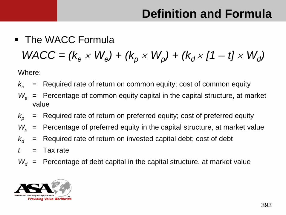
Definition and Formula
The WACC Formula WACC = (ke × We) + (kp × Wp) + (kd × [1 – t] × Wd)
Where:ke = Required rate of return on common equity; cost of common equityWe = Percentage of common equity capital in the capital structure, at market
valuekp = Required rate of return on preferred equity; cost of preferred equityWp = Percentage of preferred equity in the capital structure, at market valuekd = Required rate of return on invested capital debt; cost of debtt = Tax rateWd = Percentage of debt capital in the capital structure, at market value
393

Definition and Formula (page 185)
Invested Capital Debt Treated in this course as if it includes all interest-bearing
debt except that used for temporary seasonal purposes. Treatment of debt principal and related interest.
Interest expense associated with invested capital debt should not be a deduction in calculating invested capital cash flow.
Interest expense associated with operating debt should be a deduction in calculating invested capital cash flow.
394

Key Components of the WACC
Cost of common equity Modified CAPM or build up method
Cost of debt Market rate the business would incur on invested capital
borrowing. Sensitive to economic conditions and the company’s
ability to service debt, indicated by its capital structure and debt coverage ratios.
395
Key Components of the WACC
Cost of debt (cont’d) A particular company’s cost of debt as of the valuation
date may or may not resemble the interest rates on existing debt. Cost of debt considerations:
The current capital markets Availability and cost of debt Subject company’s current financial conditions and collateral
availability
396

Key Components of the WACC
Cost of debt (cont’d) While the cost of debt is often viewed as a simple cost of
interest relative to the amount borrowed, inclusion of compliance costs could lead to a higher cost of debt. As a certain share of offering costs is fixed relative to the
amount of funds raised, a smaller financing would also be expected to provide reduced proceeds (as a percent of the gross borrowings) relative to a larger financing.
397
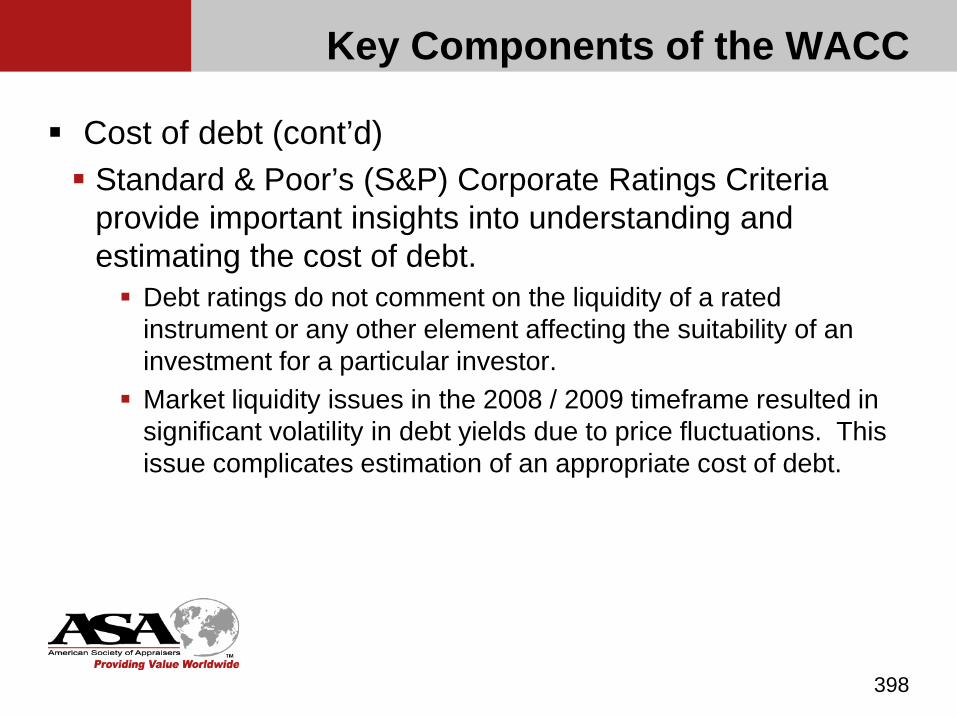
Key Components of the WACC
Cost of debt (cont’d) Standard & Poor’s (S&P) Corporate Ratings Criteria
provide important insights into understanding and estimating the cost of debt. Debt ratings do not comment on the liquidity of a rated
instrument or any other element affecting the suitability of an investment for a particular investor.
Market liquidity issues in the 2008 / 2009 timeframe resulted in significant volatility in debt yields due to price fluctuations. This issue complicates estimation of an appropriate cost of debt.
398
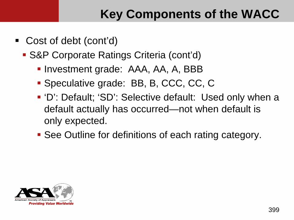
Key Components of the WACC
Cost of debt (cont’d) S&P Corporate Ratings Criteria (cont’d) Investment grade: AAA, AA, A, BBB Speculative grade: BB, B, CCC, CC, C ‘D’: Default; ‘SD’: Selective default: Used only when a
default actually has occurred—not when default is only expected. See Outline for definitions of each rating category.
399
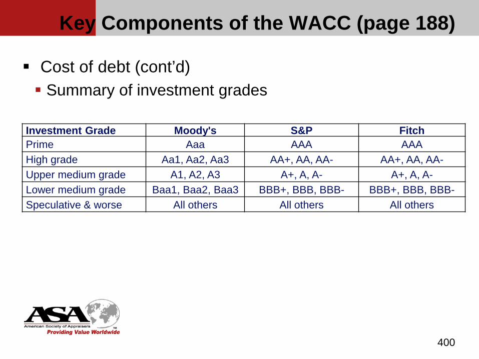
Key Components of the WACC (page 188)
Cost of debt (cont’d) Summary of investment grades
400
Investment Grade Moody's S&P FitchPrime Aaa AAA AAAHigh grade Aa1, Aa2, Aa3 AA+, AA, AA- AA+, AA, AA-Upper medium grade A1, A2, A3 A+, A, A- A+, A, A-Lower medium grade Baa1, Baa2, Baa3 BBB+, BBB, BBB- BBB+, BBB, BBB-Speculative & worse All others All others All others
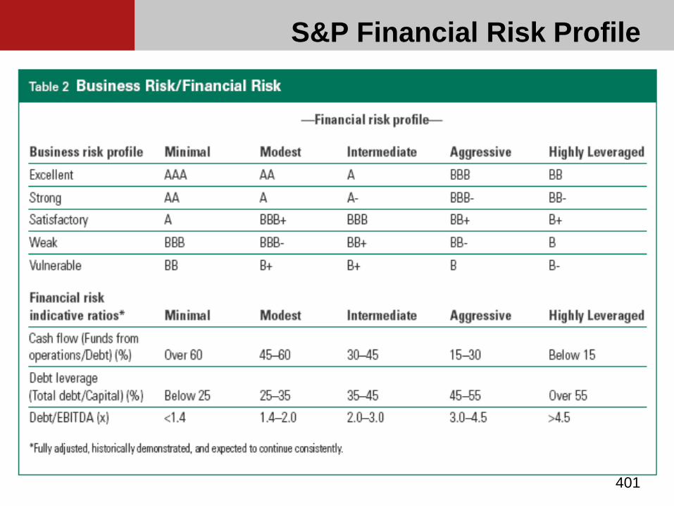
S&P Financial Risk Profile
401

Key Components of the WACC
Cost of debt (cont’d) Edward Altman Z Score and Bond Rating Equivalent Altman created the Z Score in 1968 as a predictive
measure of a company entering bankruptcy. The initial model was more suited to tangible asset
intensive companies (manufacturing). A Z Score greater than 2.99 indicates a “safe zone”
from potential bankruptcy; 1.80 to 2.99 is a “grey area”; less than 1.80 is “distress area”
402
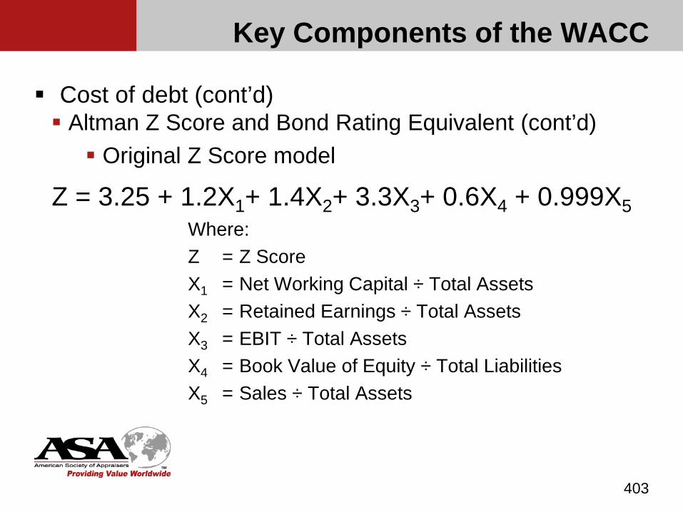
Key Components of the WACC
Cost of debt (cont’d) Altman Z Score and Bond Rating Equivalent (cont’d) Original Z Score model
Z = 3.25 + 1.2X1+ 1.4X2+ 3.3X3+ 0.6X4 + 0.999X5Where:Z = Z ScoreX1 = Net Working Capital ÷ Total AssetsX2 = Retained Earnings ÷ Total AssetsX3 = EBIT ÷ Total AssetsX4 = Book Value of Equity ÷ Total LiabilitiesX5 = Sales ÷ Total Assets
403
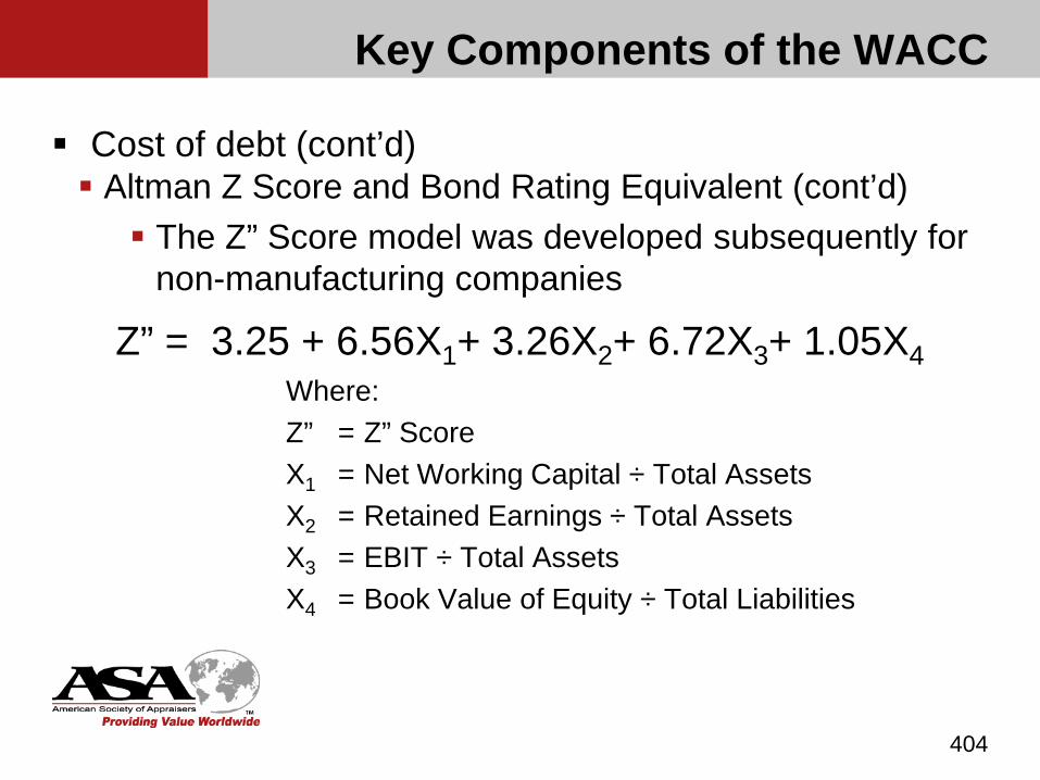
Key Components of the WACC
Cost of debt (cont’d) Altman Z Score and Bond Rating Equivalent (cont’d) The Z” Score model was developed subsequently for
non-manufacturing companies
Z” = 3.25 + 6.56X1+ 3.26X2+ 6.72X3+ 1.05X4Where:Z” = Z” ScoreX1 = Net Working Capital ÷ Total AssetsX2 = Retained Earnings ÷ Total AssetsX3 = EBIT ÷ Total AssetsX4 = Book Value of Equity ÷ Total Liabilities
404
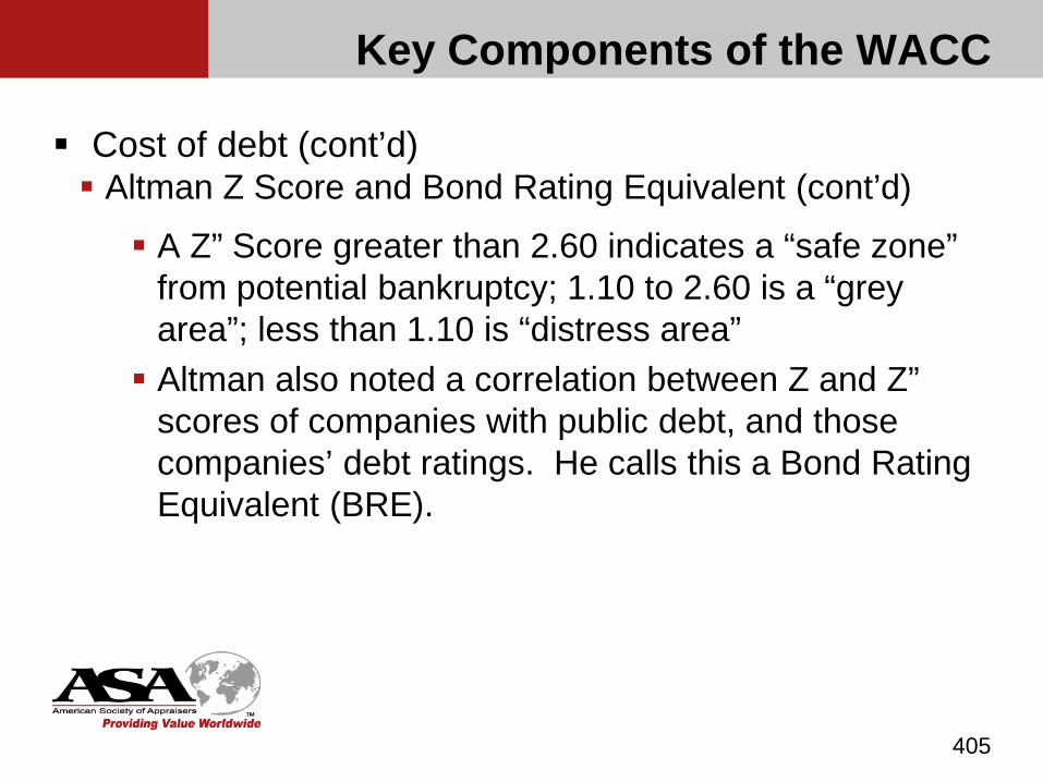
Key Components of the WACC
Cost of debt (cont’d) Altman Z Score and Bond Rating Equivalent (cont’d)
A Z” Score greater than 2.60 indicates a “safe zone” from potential bankruptcy; 1.10 to 2.60 is a “grey area”; less than 1.10 is “distress area” Altman also noted a correlation between Z and Z”
scores of companies with public debt, and those companies’ debt ratings. He calls this a Bond Rating Equivalent (BRE).
405

Altman Bond Rating Equivalent
Manufacturing/Industrial Companies
406
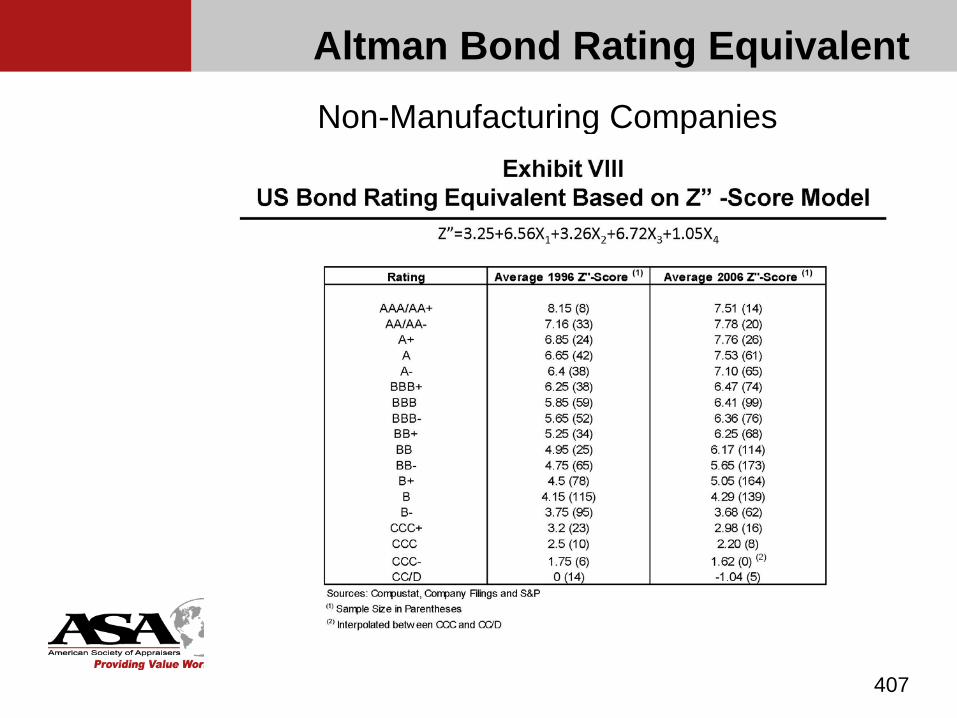
Altman Bond Rating EquivalentNon-Manufacturing Companies
407

Key Components of the WACC
Cost of debt (cont’d) Tax rate The cost of equity is an after-tax cost. Therefore, the
cost of debt in the WACC must be on an after-tax basis as well. The appropriate tax rate is the company's marginal
tax rate, expressed as a percentage of pretax income.
408
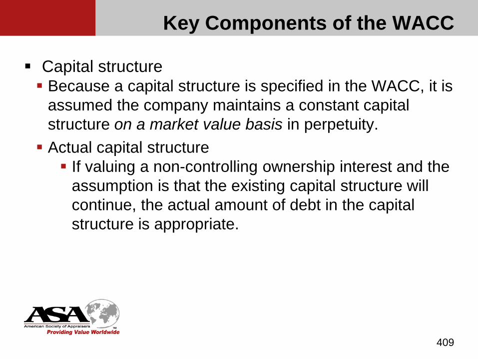
Key Components of the WACC
Capital structure Because a capital structure is specified in the WACC, it is
assumed the company maintains a constant capital structure on a market value basis in perpetuity. Actual capital structure If valuing a non-controlling ownership interest and the
assumption is that the existing capital structure will continue, the actual amount of debt in the capital structure is appropriate.
409
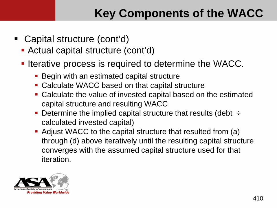
Key Components of the WACC
Capital structure (cont’d) Actual capital structure (cont’d) Iterative process is required to determine the WACC.
Begin with an estimated capital structure Calculate WACC based on that capital structure Calculate the value of invested capital based on the estimated
capital structure and resulting WACC Determine the implied capital structure that results (debt ÷
calculated invested capital) Adjust WACC to the capital structure that resulted from (a)
through (d) above iteratively until the resulting capital structure converges with the assumed capital structure used for that iteration.
410
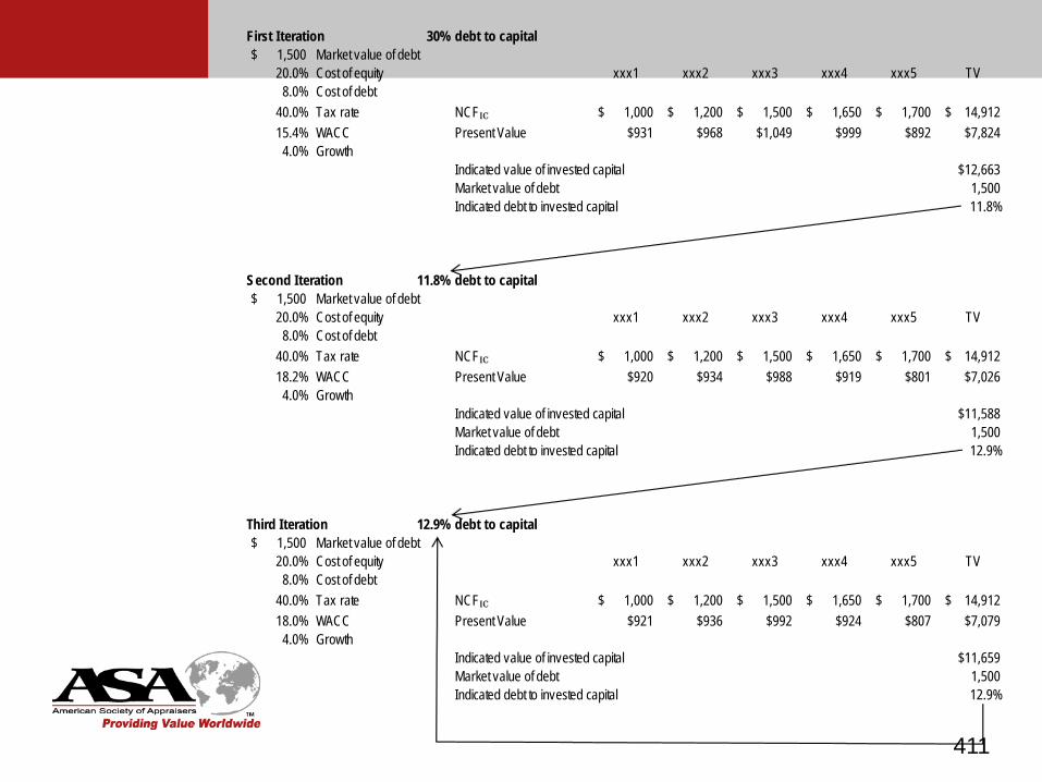
411
First I teration 30% debt to capital1,500$ Market value of debt20.0% Cost of equity xxx1 xxx2 xxx3 xxx4 xxx5 TV
8.0% Cost of debt40.0% Tax rate NCFIC 1,000$ 1,200$ 1,500$ 1,650$ 1,700$ 14,912$ 15.4% WACC Present Value $931 $968 $1,049 $999 $892 $7,824
4.0% GrowthIndicated value of invested capital $12,663Market value of debt 1,500 Indicated debt to invested capital 11.8%
Second Iteration 11.8% debt to capital1,500$ Market value of debt20.0% Cost of equity xxx1 xxx2 xxx3 xxx4 xxx5 TV
8.0% Cost of debt40.0% Tax rate NCFIC 1,000$ 1,200$ 1,500$ 1,650$ 1,700$ 14,912$ 18.2% WACC Present Value $920 $934 $988 $919 $801 $7,026
4.0% GrowthIndicated value of invested capital $11,588Market value of debt 1,500 Indicated debt to invested capital 12.9%
Third Iteration 12.9% debt to capital1,500$ Market value of debt20.0% Cost of equity xxx1 xxx2 xxx3 xxx4 xxx5 TV
8.0% Cost of debt40.0% Tax rate NCFIC 1,000$ 1,200$ 1,500$ 1,650$ 1,700$ 14,912$ 18.0% WACC Present Value $921 $936 $992 $924 $807 $7,079
4.0% GrowthIndicated value of invested capital $11,659Market value of debt 1,500 Indicated debt to invested capital 12.9%
Key Components of the WACC
Capital structure (cont’d) Hypothetical capital structure When valuing a controlling ownership interest, a
change in the capital structure may be appropriate. Optimal capital structure or market-based capital
structure
412
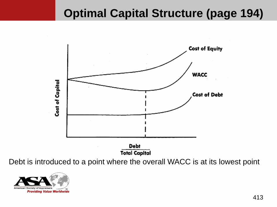
Optimal Capital Structure (page 194)
413
Debt is introduced to a point where the overall WACC is at its lowest point
Key Components of the WACC
Capital structure (cont’d) Hypothetical/optimal capital structure (cont’d)
Key considerations in estimating debt capacity are asset collateral, strength of cash flow, and industry norms. Many appraisers use industry averages based on
analysis of guideline public companies. However, public firms may differ from the subject firm
in key attributes impacting the ability to support debt.
414
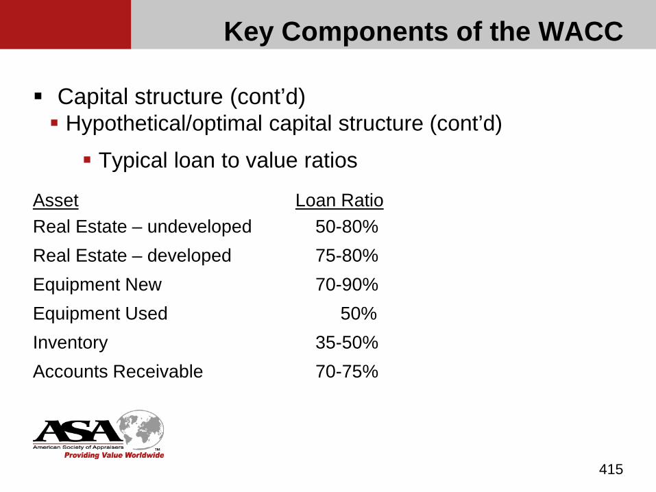
Key Components of the WACC
Capital structure (cont’d) Hypothetical/optimal capital structure (cont’d)
Typical loan to value ratios
Asset Loan RatioReal Estate – undeveloped 50-80%Real Estate – developed 75-80%Equipment New 70-90%Equipment Used 50%Inventory 35-50%Accounts Receivable 70-75%
415
Key Components of the WACC
Capital structure (cont’d) The weight of debt in the WACC is based on the market
value of the debt. Market value of debt may vary materially from its book
value Two methods to determine the market value of debt
1. Market: Guideline debt transactions2. Income: Discounted cash flows
416

Key Components of the WACC
Capital structure (cont’d) Market value of the debt (cont’d) Interest rate risk Default risk Illiquidity risk
417
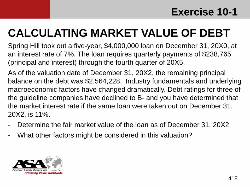
Exercise 10-1
418
CALCULATING MARKET VALUE OF DEBTSpring Hill took out a five-year, $4,000,000 loan on December 31, 20X0, at an interest rate of 7%. The loan requires quarterly payments of $238,765 (principal and interest) through the fourth quarter of 20X5.As of the valuation date of December 31, 20X2, the remaining principal balance on the debt was $2,564,228. Industry fundamentals and underlying macroeconomic factors have changed dramatically. Debt ratings for three of the guideline companies have declined to B- and you have determined that the market interest rate if the same loan were taken out on December 31, 20X2, is 11%.- Determine the fair market value of the loan as of December 31, 20X2- What other factors might be considered in this valuation?
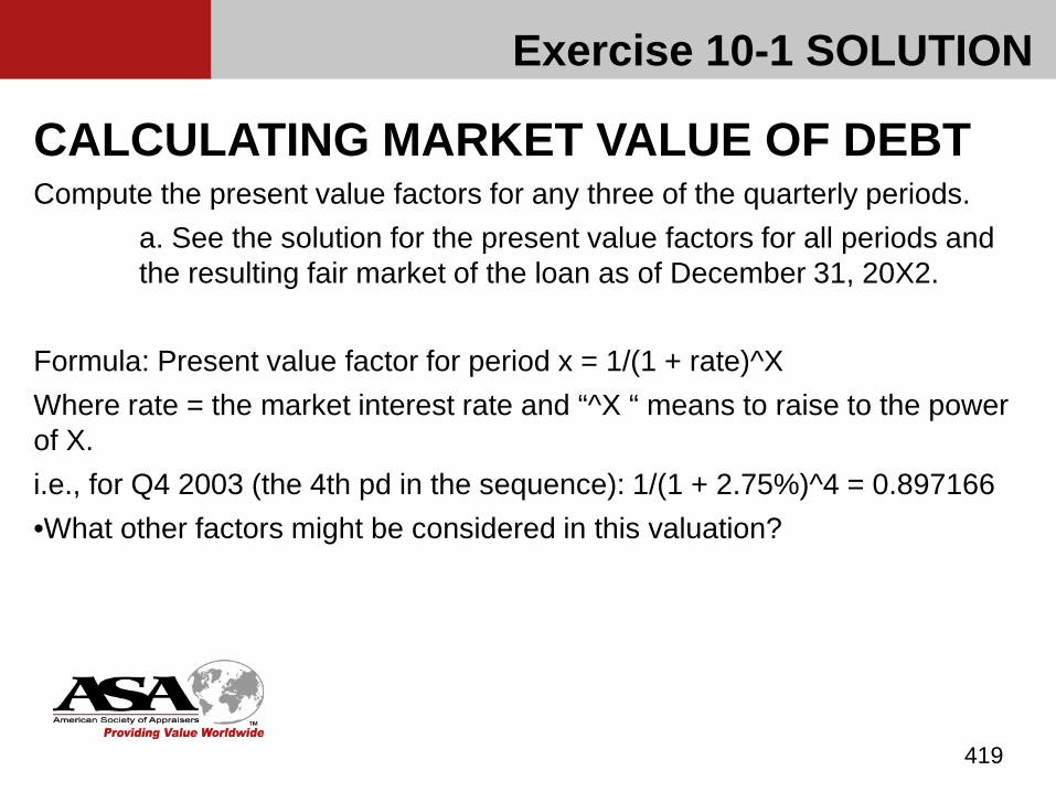
419
CALCULATING MARKET VALUE OF DEBTCompute the present value factors for any three of the quarterly periods.
a. See the solution for the present value factors for all periods and the resulting fair market of the loan as of December 31, 20X2.
Formula: Present value factor for period x = 1/(1 + rate)^XWhere rate = the market interest rate and “^X “ means to raise to the power of X.i.e., for Q4 2003 (the 4th pd in the sequence): 1/(1 + 2.75%)^4 = 0.897166•What other factors might be considered in this valuation?
Exercise 10-1 SOLUTION
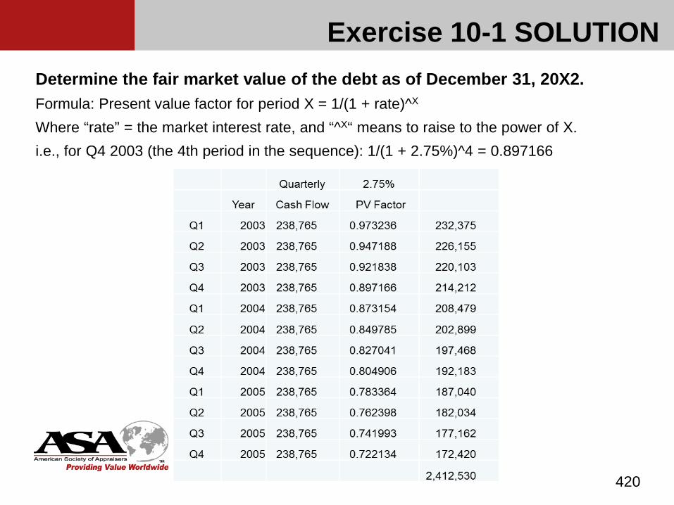
420
Determine the fair market value of the debt as of December 31, 20X2. Formula: Present value factor for period X = 1/(1 + rate)^X
Where “rate” = the market interest rate, and “^X“ means to raise to the power of X.i.e., for Q4 2003 (the 4th period in the sequence): 1/(1 + 2.75%)^4 = 0.897166
Exercise 10-1 SOLUTION

421
What other factors might be considered in this valuation?Liquidity: The value of debt is affected by interest rate risk, default risk, and liquidity risk. Valuing the remaining quarterly payments using a rate of 11% accounts for the interest rate and default risk. However, potential illiquidity of the market in general and for this specific debt may require further adjustment.
Due-on-sale or change-in-control clause: The definitions of fair value and fair market value include the assumption that a transaction does or will take place. There is growing support for the argument that the value of debt with a due-on-sale or change-in-control clause is the book value/outstanding balance plus accrued interest on the valuation date, regardless of current interest rate risks, the borrower’s credit worthiness, or market liquidity.
Exercise 10-1 SOLUTION
Application of the WACC
The WACC should be applied to invested capital net cash flow.
Since the value result from applying the WACC is invested capital, invested capital debt must be deducted to arrive at an equity value.
The cost of debt and the cost of capital used in the WACC are only relevant within a reasonable range.
422
Application of the WACC
As the percentage of debt in the capital structure increases, so will the cost of borrowing.
As the percentage of debt in the capital structure increases, so does the risk and required return on equity.
423

Exercise 10-2
424
APPLICATION OF THE WACCUsing information provided in Exhibit 10-1 (at the end of the chapter) and an equity discount rate of 22.0%, calculate the weighted average cost of capital assuming the subject of the valuation is: 10-2(a) A controlling ownership interest, and 10-2(b) A non-controlling ownership interest.
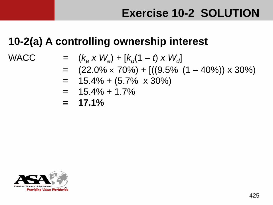
Exercise 10-2 SOLUTION
425
10-2(a) A controlling ownership interestWACC = (ke x We) + [kd(1 – t) x Wd]
= (22.0% × 70%) + [((9.5% (1 – 40%)) x 30%)= 15.4% + (5.7% x 30%)= 15.4% + 1.7% = 17.1%
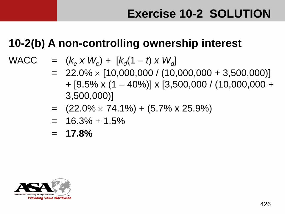
Exercise 10-2 SOLUTION
426
10-2(b) A non-controlling ownership interestWACC = (ke x We) + [kd(1 – t) x Wd]
= 22.0% × [10,000,000 / (10,000,000 + 3,500,000)] + [9.5% x (1 – 40%)] x [3,500,000 / (10,000,000 + 3,500,000)]
= (22.0% × 74.1%) + (5.7% x 25.9%)= 16.3% + 1.5% = 17.8%

Chapter 11
Pulling it All Together
427
Pulling it All Together (page 204)
428
To this point we have studied the theory behind the Income Approach, and explored the empirical data and other inputs that are used. In this Chapter we will compute the value of a 100% interest in General Delivery Trucking using all the tools we have learned.p204
In Exercise 4-7 you developed projected financial statements for GDT. In Exercise 11-1 you will determine a capitalization rate for cash flow to equity, and apply it to the resulting cash flow projections to determine a value for 100% of the shares of GDT, as of December 31, 2011, before any valuation discounts.

Pulling it All Together
429
EXERCISE 11-1
Your assignment is to compute the net present value of a 100% interest in GDT as of December 31, 2011.
Refer to Chapter 11 for instructions and information necessary to estimate a capitalization rate to apply to the cash flow to the equity of GDT, and develop an estimate of value, prior to any consideration of valuation adjustments (premiums or discounts).
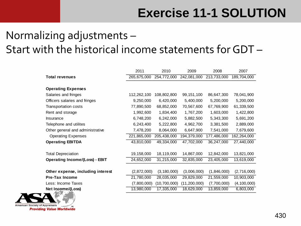
430
Normalizing adjustments –Start with the historical income statements for GDT –
2011 2010 2009 2008 2007Total revenues 265,675,000 254,772,000 242,081,000 213,733,000 189,704,000
Operating ExpensesSalaries and fringes 112,262,100 108,802,800 99,151,100 86,647,300 78,041,900Officers salaries and fringes 9,250,000 6,420,000 5,400,000 5,200,000 5,200,000Transportation costs 77,890,500 68,852,000 70,567,600 67,769,900 61,339,500Rent and storage 1,992,600 1,834,400 1,767,200 1,603,000 1,422,800Insurance 6,748,200 6,242,000 5,882,500 5,343,300 5,691,200Telephone and utilites 6,243,400 5,222,800 4,962,700 3,381,500 2,889,000Other general and administrative 7,478,200 8,064,000 6,647,900 7,541,000 7,679,600
Operating Expenses 221,865,000 205,438,000 194,379,000 177,486,000 162,264,000Operating EBITDA 43,810,000 49,334,000 47,702,000 36,247,000 27,440,000
Total Depreciation 19,158,000 18,119,000 14,867,000 12,842,000 13,821,000Operating Income/(Loss) - EBIT 24,652,000 31,215,000 32,835,000 23,405,000 13,619,000
Other expense, including interest (2,872,000) (3,180,000) (3,006,000) (1,846,000) (2,716,000)Pre-Tax Income 21,780,000 28,035,000 29,829,000 21,559,000 10,903,000Less: Income Taxes (7,800,000) (10,700,000) (11,200,000) (7,700,000) (4,100,000)Net Income/(Loss) 13,980,000 17,335,000 18,629,000 13,859,000 6,803,000
Exercise 11-1 SOLUTION

Exercise 11-1 SOLUTION
Normalization adjustments to the historical financial statements –(Note – this shows only those items for which the 2011 results are impacted –that is, since the adjustment for litigation costs does not impact 2011, it is omitted from the table below)
431
2011 2010 2009 2008 2007Officers salaries and fringes 9,250,000 6,420,000 5,400,000 5,200,000 5,200,000Adjustments (7,000,000) (4,636,596) (3,705,433) (3,703,869) (3,872,072) Adjusted 2,250,000 1,783,404 1,694,567 1,496,131 1,327,928
Other general and administrative 7,478,200 8,064,000 6,647,900 7,541,000 7,679,600Adjustments (400,000) (600,000) (1,200,000) (3,600,000) (6,800,000) Adjusted 7,078,200 7,464,000 5,447,900 3,941,000 879,600
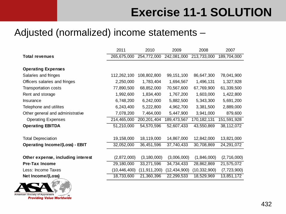
Adjusted (normalized) income statements –
432
2011 2010 2009 2008 2007Total revenues 265,675,000 254,772,000 242,081,000 213,733,000 189,704,000
Operating ExpensesSalaries and fringes 112,262,100 108,802,800 99,151,100 86,647,300 78,041,900Officers salaries and fringes 2,250,000 1,783,404 1,694,567 1,496,131 1,327,928Transportation costs 77,890,500 68,852,000 70,567,600 67,769,900 61,339,500Rent and storage 1,992,600 1,834,400 1,767,200 1,603,000 1,422,800Insurance 6,748,200 6,242,000 5,882,500 5,343,300 5,691,200Telephone and utilites 6,243,400 5,222,800 4,962,700 3,381,500 2,889,000Other general and administrative 7,078,200 7,464,000 5,447,900 3,941,000 879,600
Operating Expenses 214,465,000 200,201,404 189,473,567 170,182,131 151,591,928Operating EBITDA 51,210,000 54,570,596 52,607,433 43,550,869 38,112,072
Total Depreciation 19,158,000 18,119,000 14,867,000 12,842,000 13,821,000Operating Income/(Loss) - EBIT 32,052,000 36,451,596 37,740,433 30,708,869 24,291,072
Other expense, including interest (2,872,000) (3,180,000) (3,006,000) (1,846,000) (2,716,000)Pre-Tax Income 29,180,000 33,271,596 34,734,433 28,862,869 21,575,072Less: Income Taxes (10,446,400) (11,911,200) (12,434,900) (10,332,900) (7,723,900)Net Income/(Loss) 18,733,600 21,360,396 22,299,533 18,529,969 13,851,172
Exercise 11-1 SOLUTION
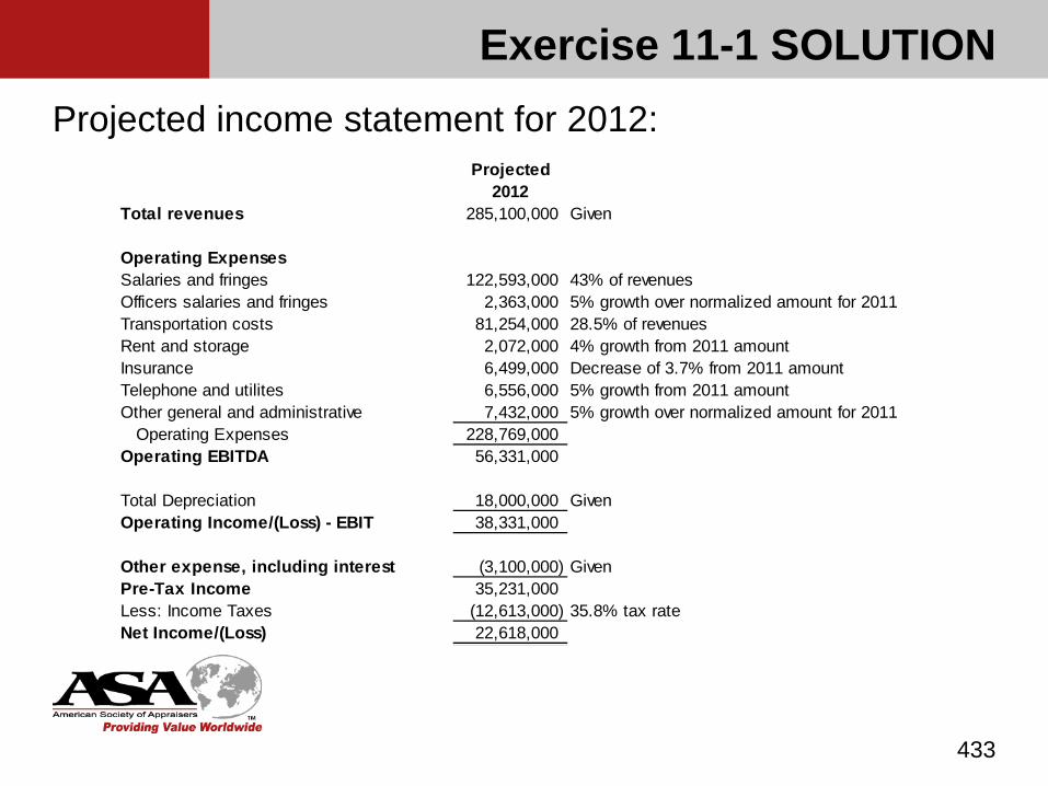
Projected income statement for 2012:
433
Projected2012
Total revenues 285,100,000 Given
Operating ExpensesSalaries and fringes 122,593,000 43% of revenuesOfficers salaries and fringes 2,363,000 5% growth over normalized amount for 2011Transportation costs 81,254,000 28.5% of revenuesRent and storage 2,072,000 4% growth from 2011 amountInsurance 6,499,000 Decrease of 3.7% from 2011 amountTelephone and utilites 6,556,000 5% growth from 2011 amountOther general and administrative 7,432,000 5% growth over normalized amount for 2011
Operating Expenses 228,769,000Operating EBITDA 56,331,000
Total Depreciation 18,000,000 GivenOperating Income/(Loss) - EBIT 38,331,000
Other expense, including interest (3,100,000) GivenPre-Tax Income 35,231,000Less: Income Taxes (12,613,000) 35.8% tax rate Net Income/(Loss) 22,618,000
Exercise 11-1 SOLUTION
Note that this is an oversimplification for the purposes of this Exercise. In practice, individual line items of the income statement must be projected as far into the future as needed to assure stable long-term growth.
434
Exercise 11-1 SOLUTION
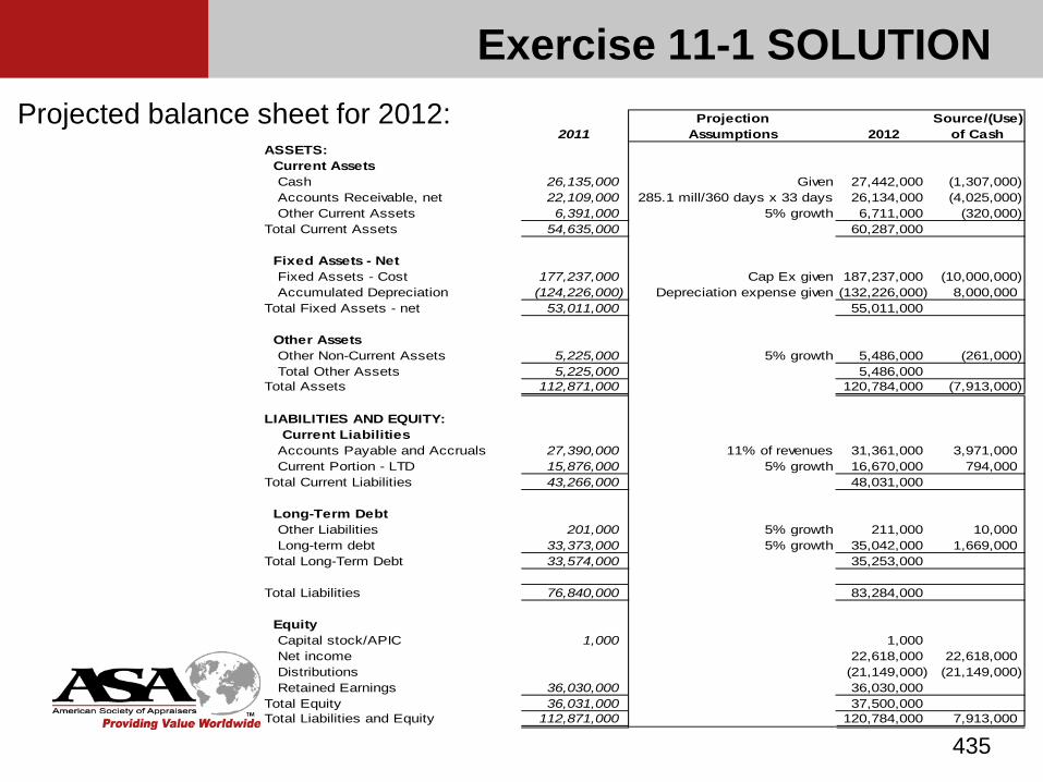
Projected balance sheet for 2012:
435
Projection Source/(Use)2011 Assumptions 2012 of Cash
ASSETS: Current Assets
Cash 26,135,000 Given 27,442,000 (1,307,000)Accounts Receivable, net 22,109,000 285.1 mill/360 days x 33 days 26,134,000 (4,025,000)Other Current Assets 6,391,000 5% growth 6,711,000 (320,000)
Total Current Assets 54,635,000 60,287,000
Fixed Assets - NetFixed Assets - Cost 177,237,000 Cap Ex given 187,237,000 (10,000,000)Accumulated Depreciation (124,226,000) Depreciation expense given (132,226,000) 8,000,000
Total Fixed Assets - net 53,011,000 55,011,000
Other AssetsOther Non-Current Assets 5,225,000 5% growth 5,486,000 (261,000)Total Other Assets 5,225,000 5,486,000
Total Assets 112,871,000 120,784,000 (7,913,000)
LIABILITIES AND EQUITY: Current Liabilities
Accounts Payable and Accruals 27,390,000 11% of revenues 31,361,000 3,971,000Current Portion - LTD 15,876,000 5% growth 16,670,000 794,000
Total Current Liabilities 43,266,000 48,031,000
Long-Term DebtOther Liabilities 201,000 5% growth 211,000 10,000Long-term debt 33,373,000 5% growth 35,042,000 1,669,000
Total Long-Term Debt 33,574,000 35,253,000
Total Liabilities 76,840,000 83,284,000
EquityCapital stock/APIC 1,000 1,000Net income 22,618,000 22,618,000Distributions (21,149,000) (21,149,000)Retained Earnings 36,030,000 36,030,000
Total Equity 36,031,000 37,500,000Total Liabilities and Equity 112,871,000 120,784,000 7,913,000
Exercise 11-1 SOLUTION
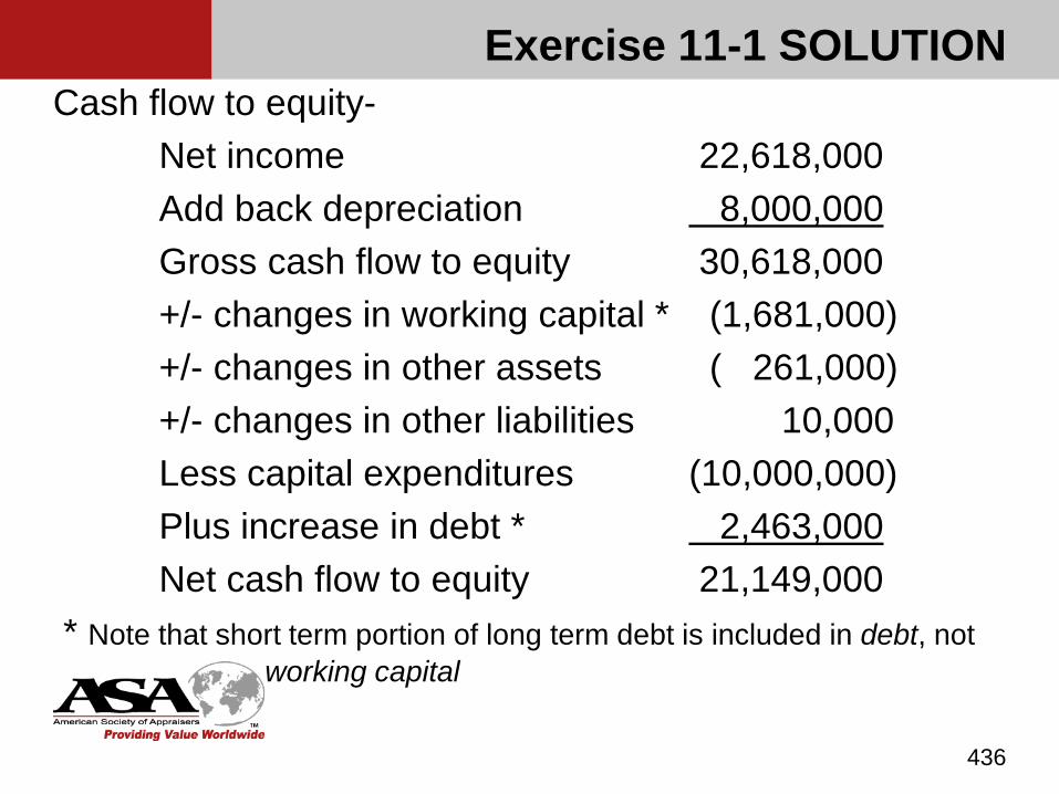
Cash flow to equity-Net income 22,618,000Add back depreciation 8,000,000Gross cash flow to equity 30,618,000+/- changes in working capital * (1,681,000)+/- changes in other assets ( 261,000)+/- changes in other liabilities 10,000Less capital expenditures (10,000,000)Plus increase in debt * 2,463,000Net cash flow to equity 21,149,000
* Note that short term portion of long term debt is included in debt, not working capital
436
Exercise 11-1 SOLUTION
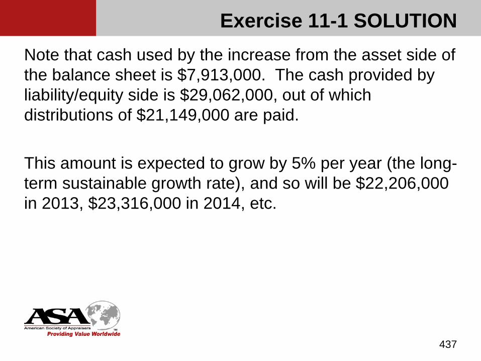
Note that cash used by the increase from the asset side of the balance sheet is $7,913,000. The cash provided by liability/equity side is $29,062,000, out of which distributions of $21,149,000 are paid.
This amount is expected to grow by 5% per year (the long-term sustainable growth rate), and so will be $22,206,000 in 2013, $23,316,000 in 2014, etc.
437
Exercise 11-1 SOLUTION

This amount is expected to grow by 5% per year (the long-term sustainable growth rate), and so will be $22,206,000 in 2013, $23,316,000 in 2014, etc.
Note that this is an oversimplification for the purposes of this Exercise. In practice, individual line items of the balance sheet must be projected as far into the future as the projected income statements.
438
Exercise 11-1 SOLUTION

Developing the Discount RateExhibits B-2 (Book value of equity), B-3 (5-year average net income) and B-5 (Total assets) were used in this example solution, with the results below, using a simple average of the three Exhibits:
439
D&PExhibit
B-2 Book value of equity = $36 million is the 25th portfolio 6.18%
B-3 5-year average (adjusted) net income = $18,463,300, 23rd portfolio 5.79%
B-5 Total assets = $112,871,000, 25th portfolio 6.69%
Selected Risk Premium for Size (average of the three) 6.22%
Exercise 11-1 SOLUTION
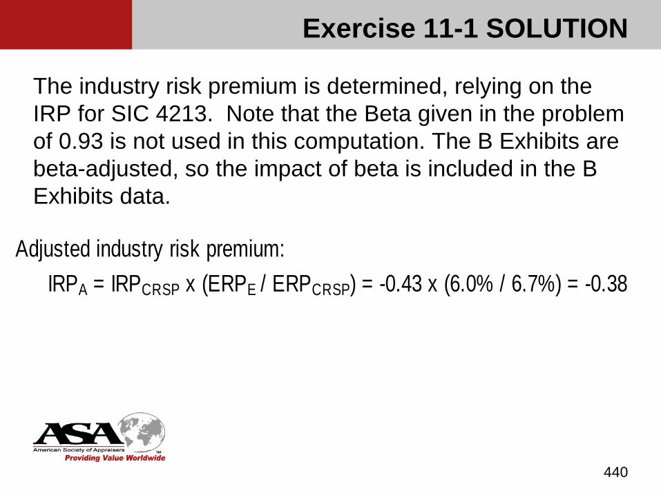
The industry risk premium is determined, relying on the IRP for SIC 4213. Note that the Beta given in the problem of 0.93 is not used in this computation. The B Exhibits are beta-adjusted, so the impact of beta is included in the B Exhibits data.
440
Adjusted industry risk premium:IRPA = IRPCRSP x (ERPE / ERPCRSP) = -0.43 x (6.0% / 6.7%) = -0.38
Exercise 11-1 SOLUTION
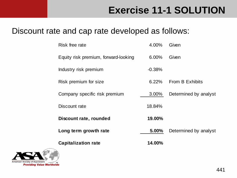
Discount rate and cap rate developed as follows:
441
Risk free rate 4.00% Given
Equity risk premium, forward-looking 6.00% Given
Industry risk premium -0.38%
Risk premium for size 6.22% From B Exhibits
Company specific risk premium 3.00% Determined by analyst
Discount rate 18.84%
Discount rate, rounded 19.00%
Long term growth rate 5.00% Determined by analyst
Capitalization rate 14.00%
Exercise 11-1 SOLUTION
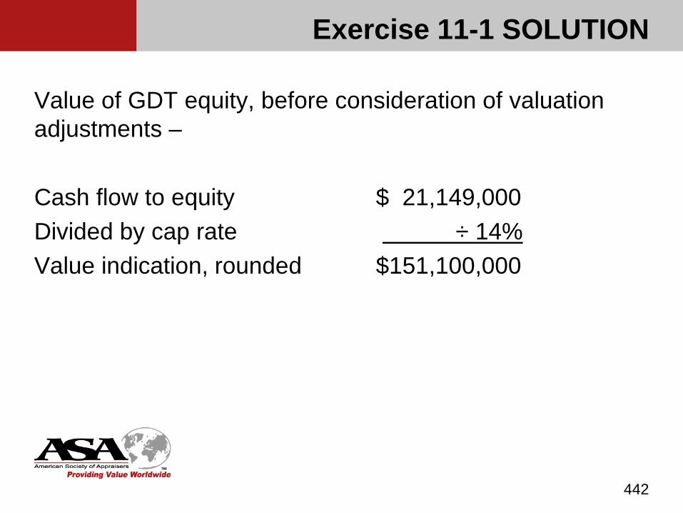
Value of GDT equity, before consideration of valuation adjustments –
Cash flow to equity $ 21,149,000Divided by cap rate ÷ 14%Value indication, rounded $151,100,000
442
Exercise 11-1 SOLUTION

Chapter 12
Levels of Value
443
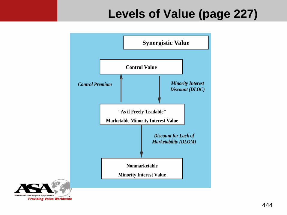
Levels of Value (page 227)
444
Levels of Value
Control Value
Control Premium Minority Interest Discount (DLOC)
“As if Freely Tradable”
Marketable Minority Interest Value
Discount for Lack of Marketability (DLOM)
Nonmarketable
Minority Interest Value
Test Synergistic Value
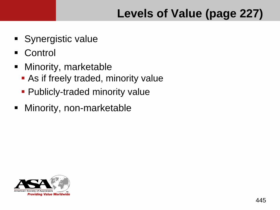
Levels of Value (page 227)
Synergistic value Control Minority, marketable As if freely traded, minority value Publicly-traded minority value
Minority, non-marketable
445

Methodologies and Levels of Value
446
Approach/Method Assumptions Resulting ValueIncome approach Control cash flows
Minority cash flowsControl *Minority, marketable
Merger & acquisition
Guideline public company
Control transacted
Control cash flowsMinority cash flows
Control *
Control *Minority, marketable
Asset accumulation method
Excess earnings method
Control over assets
Control over assets
Control *
Control *
* - for control level of value, synergies could indicate investment value
Level of Value-Income Approach
Minority or Control? Discount rates are derived from returns generated by
minority interests in public companies. The returns measured in the market include some control
transactions. If control adjustments are made to the benefit stream, it is
reasonable to believe that applying a market-derived discount rate yields a minority basis of value?
447
Level of Value-Income Approach
Minority or Control (cont’d)? Management of publicly traded companies have different
motivation (maximizing shareholder value) than those of closely held companies (maximizing after-tax owner’s discretionary income). Publicly traded companies management and boards are
subject to oversight and scrutiny (e.g., SEC, DOJ, large-block holders, independent boards, auditors).
448
Level of Value-Income Approach
Minority or Control (cont’d)? Today, the level of value yielded by income approach
methods is considered to depend on the character of the income stream discounted or capitalized. If adjustments have been made to reflect the cash flow
that only a controlling shareholder can access, then the value derived is control. If the cash flow is only what is actually available to a
minority shareholder, then the value derived is minority.
449
Level of Value-Income Approach
Minority or Control (cont’d)? Note that, in some cases, additional adjustments may be
needed for control issues not reflected in cash flow. Even if there is full pro rata distribution of control level
cash flow, the minority interest may still warrant a discount. If all cash flow is diverted to the controlling shareholder,
the minority interest value may still not be zero.
450

Level of Value-Income Approach
Marketable or Non-marketable? The income approach is assumed to yield a marketable
value. Discount rates are derived from returns in the public
market, where securities have relatively instant liquidity. The projected income stream is assumed to be
immediately transferable.
451

Level of Value-Income Approach
Marketable or Non-marketable (cont’d)? Some practitioners increase the discount rate to account
for perceived marketability factors in the subject. It is preferable to separate the analysis of marketability
factors and address them explicitly in a lack of marketability discount.
452

Level of Value-Income Approach
The income approach level of value will therefore usually be “control” or “minority, marketable” If the initial conclusion is a control value, it is possible to
reach a minority, non-marketable value by applying a discount for lack of control and a discount for lack of marketability (“indirect method”). If the initial conclusion is a minority, marketable value, it
is possible to reach a minority, non-marketable value by applying a discount for lack of marketability (“direct method”).
453
Level of Value-Income Approach
Marketability vs. liquidity Liquidity: the ability to convert an asset…into cash
without significant loss of principal Marketability: the capability and ease of transfer or
salability of an asset
454

Sequential Nature of Discounts
The DLOC and DLOM should be applied sequentially. They are not additive.
Control value $100- DLOC (30% x $100) -30= Minority as if freely-traded 70= DLOM (20% x $70) -14= Minority, non-marketable $ 56
Effective combined discount 44%
455

EXAM REVIEW
456
Exam Tips
Read each question completely and carefully. Answer the question being asked. Do not read too much into the question; there are
no intentionally tricky questions. There may be some rounding errors on the
calculation problems. Choose the closest answer provided.
Each question carries the same weight (1 point).
457