Buyer Size, Price Discrimination, and Quality Differentiation inInternational Trade∗

Anna Ignatenko†

November 11, 2019

Please click here for the most recent version

Abstract

A surprising finding from firm-level customs data is that, in violation of the Law of One Price,different buyers of imported inputs pay different prices. The literature has attributed this fullyto differences in the quality of inputs. Instead, in this paper I argue that this phenomenon canbe explained by price discrimination in the input market. Using a unique dataset that identifiesboth the sellers and the buyers and provides detailed descriptions of the transacted products, Ifind substantial variation in prices charged by the same seller for the same product. I rationalizethis finding by introducing oligopolistic input producers to a standard trade model, and showthat the ability to backwards integrate allows larger buyers to obtain lower input prices. Myanalysis suggests that productivity gains from trade differ across firms and depend on the prices,quality and variety of inputs imported by a firm. It also implies that consumer gains from tradeare larger under price discrimination in input markets.

JEL codes: F10, F11, F14, F23, L11Key words: price discrimination, vertical integration, buyer size, oligopoly, imported inputs

∗Acknowledgements: I am very thankful to my advisors, Rob Feenstra, Andre Boik, Deborah Swenson, andAlan Taylor for their invaluable guidance and encouragement. I would also like to thank Andrew Atkeson, LorenzoCaliendo, Hiroyuki Kasahara, Monica Morlacco, Kadee Russ, Ina Simonovska, Sanjay Singh, participants of RIDGEDecember Forum 2018, Sardinian Empirical Trade Conference, Hitotsubashi International Trade and InvestmentWorkshop, and UC Davis International/Macro Brownbags for helpful comments and suggestions. I am especiallygrateful to Rob Feenstra for providing funding for data acquisition. All errors are mine.

†Department of Economics, University of California, Davis, One Shields Avenue, Davis, CA 95616; e-mail: aig-natenko@ucdavis.edu

1

1 Introduction

In the face of new and more granular firm-level data, a recurring finding is that firms chargedifferent prices to different buyers: a violation of the Law of One Price. The existing trade literaturehas overwhelmingly explained this through a theory that different destination countries demanddifferent qualities of goods, and that the price variation across buyers is accounted for by differencesin qualities. In other words, the Law of One Price is not in fact violated because the goods beingsold are different. However, another and perhaps even more natural explanation for the firm-to-firm price variation, is that the goods are in fact the same but firms discriminate across differentbuyers. This alternative explanation for the price patterns in trade has been demonstrated to bevalid in the firm-to-end-consumer context by Simonovska (2015), and has been studied extensivelyin an industrial organization literature that dates back as early as Robinson (1933). It wouldalso seem natural then that discrimination could also occur in firm-to-firm transactions, which hasbeen studied by industrial organization economists since at least Katz (1987). There are countlessanecdotal examples of different firms obtaining different input prices from domestic suppliers: Wal-Mart, for example, is notorious for their lower input prices for identical goods. This paper arguesthat the variation of prices across buyers, conditional on the product’s quality, is systematic ininternational firm-to-firm transactions.

In this paper, I use a new matched importer-exporter customs dataset from Paraguay to studythe determinants of price variation across importers. To illustrate my main motivating finding,Figure 1 displays the extent of variation of unit-values across firms importing the same product(defined as an 8-digit Harmonized system, HS8, code) from the same seller. The documentedvariation is surprisingly large, with the average coefficient of variation of about 65%. I show thatthis variation is not entirely driven by the differences in quality of products by using extremelynarrow product definitions at the level of brand and detailed commercial descriptions uniquelyavailable in the new customs dataset from Paraguay. Furthermore, I find that conditional onquality, product prices vary systematically with the importer size: larger importers and importerspurchasing in larger volumes consistently pay lower prices.

To rationalize these findings, I build a novel model of international trade, in which price dis-crimination arises as a result of strategic interaction of buyers and sellers of inputs. Buildingon the idea proposed in Katz (1987), in this model the production of final goods requires inputsthat downstream producers can either buy from upstream producers and/or produce themselves.Learning the upstream technology is costly, and thus only more productive downstream firms findit worthwhile to produce inputs in-house. Because they can always substitute their own inputs forthe expensive ones, firms that “backwards integrate” are more elastic to changes in inputs prices.Since input producers set prices inversely proportional to firm’s demand elasticity, more productivedownstream firms are predicted to obtain better input prices. Intuitively, the threat of losing largebuyers, which can switch to their own inputs, is what makes input producers lower the prices theycharge to large buyers.

2

Figure 1: Unit values of imported goods sold by the same seller vary across importers

Note that buyer size has radically different implications for prices in the intermediate goods andfinal goods markets. In the later, consumers with higher willingness to pay are known to be chargedhigher prices (e.g. Simonovska (2015), Jung et al. (2015) in international trade literature, andGerardi and Shapiro (2009), Chandra and Lederman (2015) in industrial organization literature).This paper suggests that this is because consumers, unlike final goods producers, can not crediblythreaten the sellers with “backwards integration”.

This paper is the first to rationalize the existence of third-degree price discrimination in firm-to-firm international trade transactions. The fist main insight of the proposed theoretical model is thatmore efficient firms have a viable threat of substitution when negotiating the price with any seller.The importance of intra-firm trade in global trade flows (e.g. Bernard et al. (2009)) suggests that“backwards integration” can be a natural threat point for many importers. International tradeliterature also offers other mechanisms resulting in more efficient firms to have more attractivealternative options of sourcing inputs. More efficient firms can afford to search more and findbetter suppliers (e.g. Bernard et al. (2015)). Larger importers can afford to pay fixed costs ofimporting from many more countries (e.g. Antras et al. (2017)). In line with these mechanisms,the main prediction of this paper can be interpreted more broadly as following: firms with largerextensive margin of sourcing are able to negotiate lower prices from their suppliers.

The second insight is that as importing firms import goods of varying quality and face differentprices conditional on the same quality, productivity gains from trade are heterogeneous acrossbuyers. Under CES production function, I apply the logic similar to Feenstra (1994) to decomposefirm productivity into four components: exogenous productivity draw, price, quality and variety of

3

imported inputs. Since larger firms are charged lower mark-ups due to price discrimination in inputmarkets, they experience larger cost-shock pass-through. In other words, larger firms gain morefrom trade liberalization, and the overall gains from trade depend on the distribution of firm sizein equilibrium. Specifically, more concentrated downstream sectors are expected to obtain largergains from trade liberalization in the upstream sector.

I also study the implications of price discrimination in input markets for final goods consumers.In industries with free entry, the larger extent of price discrimination in input markets leads tohigher expected profits of the downstream firms and fewer active firms on the market in equilibrium.Since only the most productive firms remain on the market, it benefits final goods consumersthrough lower prices of final goods.

The reminder of the paper is organized as follows. In Section 2, I document price variation infirm-to-firm transactions that is consistent with the existence of price discrimination. In Section 3,I introduce a new model of trade that explains such variation. In Section 4, I study the implicationsof price discrimination for the gains from trade, and in Section 5 I conclude.

2 Data and Stylized Facts

2.1 Data

The main dataset consists of the entire universe of import and export transactions of Paraguayanfirms over the period 2013 - 2018. For each transaction, the data records information on the prod-uct transacted, free-on-board (FOB) and customs-insurance-freight (CIF) values (in US dollars),gross and net weight (in kilograms), quantity (in units), the date of transaction, as well as theimporting/exporting firm’s unique identifier. In contrast to many other firm-level customs datasets, the Paraguayan data also includes the name of the foreign supplier of imported goods, whichI have cleaned and standardizing following the procedure described in Appendix A. Each importtransaction is thus identified with a buyer identifier (b), a product code at the HS 8-digit level ofdisaggregation (p), a supplier name (s), a (foreign) country of purchase (c), and a date (t). On theother hand, each export transaction is described with an exporter identifier, a product code at theHS 8-digit level of disaggregation, a date, and a destination country.

Table 1 shows that, as in most developing countries, there are a lot more importing firms andimport transactions than exporting firms and export transactions in Paraguay a year. While, onaverage, more than 6 000 firms engage in importing per year, only a thousand firms engage inexporting with 650 of them both importing and exporting. This results in more than 600 000import transaction per year, and only 105 000 export transactions per year.

Both importers and exporters exhibit substantial heterogeneity in their size and sourcing/exportingstrategies. An average importer imports 158 HS 8-digit products a year and sources imports from7 different countries, while an average exporter exports 14 different HS 8-digit products to 10destination countries. Importers that also export, on average, import more HS8 products, source

4

goods from more countries, and, in general, have higher import expenditures than non-exportingimporters. Exporting importers comprise only about 10% of importing firms, by count, but accountfor one third of the observed import transactions in the data.

mean sd p10 p25 p50 p75 p90Importers

# Importers/Year 6 159 282 5 524 6 083 6 273 6 373 6 408# HS8 products/Year-Firm 158 147 15 39 106 244 409# Countries/Year-Firm 7 6 1 2 5 11 16FOB Value (’000 $US)/Year-Firm 12 441 22 792 246 982 3 982 15 187 32 888N/Year 630 714N 3 730 018

Exporters# Exporters/Year 1 053 47 1 000 1 013 1 045 1 071 1 128# HS8 products/Year-Firm 14 15 2 4 11 17 25# Destinations/Year-Firm 10 12 1 3 4 11 30FOB Value (’000 $US)/Year-Firm 58 060 105 347 701 3 272 22 984 55 147 224 089N/Year 105 452N 589 605

Importers-Exporters# Firms/Year 651 35 596 626 654 668 709# HS8 products/Year-Importer 214 163 28 67 172 341 457# Countries/Year-Importer 11 7 2 6 11 16 21FOB Value (’000 $US)/Year-Importer 20 968 24 671 1 152 3 682 13 367 29 707 48 617# HS8 products/Year-Exporter 15 26 1 2 5 16 46# Destinations/Year-Exporter 4 5 1 1 2 4 7FOB Value (’000 $US)/Year-Exporter 11 482 49 335 4 33 209 1 722 29 511N/Year 627 866N 1 062 048

Table 1: Summary Statistics, 2013 - 2018

Most import and export transactions involve intermediate goods, as defined by the UN Classifi-cation of Broad Economic Caterogies (BEC). classification. Table 2 shows that intermediate goodscomprise 50% of import and 58% of export transaction and account for 35% and 40% of the totalyearly (FOB) value of imports and exports, respectively. As an agricultural economy, Paraguayimports mostly differentiated products (by value), and exports mostly homogeneous products (ref-erence prices and goods traded on organized exchanges), as defined in the Rauch classification(Rauch (1999)).

In this paper, I study the determinants of import price variation across importers, yet the datadoes not record per-unit prices of imported goods. Following the literature, I first compute unitvalues as ratios of FOB value over volume imported as proxies for prices of imported goods:

pbspt = V aluebspt/V olumebspt,

where the data provides two measures of volume - physical units and physical weight (gross and netof packaging weight). Since unit values are known to be a noisy measure of prices, below I discuss

5

Imported goods Exported goodsBy count, % By FOB value, % By count, % By FOB value, %

Consumption 27 20 22 4Capital 14 22 2 1Intermediate 50 35 58 40Differentiated 83 59 71 14Reference priced 12 20 6 3Traded 1 3 21 45

Table 2: Imported and exported goods, by type, 2013 - 2018.

the potential sources of the measurement error and how I use my data to address them and, incertain cases, compute unit values very closely resembling per-unit prices.

A major critique of using unit values as a proxy for prices is that quality differences betweengoods and ”hidden” varieties are not accounted for. When an actual product transacted is unknown,then differences in unobserved product characteristics and/or quality within a broad HS categorycan make problematic the comparison of unit values across importers. To mitigate this problem, Imake use of the uniquely detailed nature of product descriptions available in the data. First, partfrom a country of purchase and a detailed HS 8-digit product code, the data includes the nameof the seller in the foreign country and brand name of the product. Table 3 shows that acrossall 36 823 HS8-Country product categories only 10% are supplied by the only seller and come inonly 2 different brands. The median number of sellers per HS8-Country category is equal to 16

for all products, 18 - for differentiated products, and 7 and 4 - for reference priced and traded onorganized exchanges products, respectively. The large number of suppliers within HS8-Countrycategories, even among relatively homogeneous products, can only be sustained if there is enoughproduct differentiation by the seller.In this case, seller identifier should be included in the productdefinition. Since 75% of foreign sellers supply only one brand within an HS8 product category,defining a product as an HS8-seller combination, will take into account brand differentiation withinHS8-Country product categories.

When individual products are defined as an HS8-seller combination, the number of productsincreases to 158 294, which substantially limited the extent of within product differentiation. Atthis level of disaggregation, the only remaining source of measurement error in the unit values canbe due to sellers vertically differentiating products within HS 8-digit codes across buyers. To assessthe relevance of this concern, I rely on word descriptions of products provided by foreign sellers.According to customs regulation in Paraguay, commercial invoices upon importing must includea full and accurate (non-generic) descriptions of goods and their country of origin (which canbe different from the source country). Table 4 provides several examples of product descriptions(translated from Spanish to English) and brand names that I obtain after applying methods oftextual data cleaning to them (for details, see Appendix A). It suggests that in some cases, productdescriptions can be used to identify different varieties within a given HS8-seller or HS8-seller-brand

6

mean sd count p10 p25 p50 p75 p90

Number of sellers per HS8-Country

All products 27 30 36 823 2 5 16 40 70

Differentiated 29 30 28 693 2 6 18 43 73Reference priced 16 24 6 351 1 3 7 19 43Traded 6 5 506 1 2 4 8 13

Number of brand names per HS8-Country

All products 35 59 36 823 2 5 16 40 81

Differentiated 38 62 28 693 2 6 17 43 86Reference priced 15 19 6 351 1 3 8 19 42Traded 7 9 506 1 2 4 8 14

Number of brand names per HS8-Seller

All products 4 13 158 294 1 1 1 2 5

Differentiated 4 14 135 192 1 1 1 2 6Reference priced 2 3 17 643 1 1 1 2 4Traded 2 2 1 064 1 1 1 2 3

Table 3: Within HS8-Country product differentiation, 2013 - 2018.

combinations.

HS code Seller Description Brand32149000 Autocolor LTDA Mortar type ACI 20 kg bag Votorantim32149000 Autocolor LTDA Mortar type ACI 20 kg bag Quartzolit33021000 Bebidas Refrescantes Acid solution colorants Coca-Cola33021000 Bebidas Refrescantes Aspartame Coca-Cola33051000 Euro 2000 SA Shampoo Keratin Lift x 960cc Question Professional33051000 Euro 2000 SA Shampoo Nutrition x 960cc Question Professional33051000 Euro 2000 SA Shampoo Retention x 960cc Question Professional84833029 Data Tech Inc Vehicle bearings Ford84833029 Data Tech Inc Vehicle bearings Toyota87019490 Agco Maq Agricola Tractor model A990 4x4 yellow 2017 Valtra87019490 Agco Maq Agricola Tractor model A750 4x4 yellow 2017 Valtra87019490 Agco Maq Agricola Tractor model BM110 4x4 yellow 2017 Valtra

Table 4: Examples of brands and commercial descriptions in the data

7

The second concern that can cause measurement error in the unit value proxies for prices isimprecision with which the volume of trade is recorded. Physical units can be reported by theseller in any unit type1, which makes the comparison of unit values across transactions problem-atic. Physical weight, on the other hand, is required to be reported in kilograms, which makes ituniformity across a more suitable measure of volume. However, if unit weight (weight/quantity)varies substantially across sub-varieties within HS8-seller categories, it can lead to imprecise unitvalues. To minimize the measurement error in the unit values, for each HS8-seller combination, Ichoose the measure of volume of trade which minimizes the within HS8-seller coefficient of variationof unit values. Although this procedure helps reducing the measurement error at the HS8-sellererror, it can make unit values incomparable across different sellers of the same HS8 product cate-gory, if they use different units to measure the volume of trade. It is not a problem for the mainresults, as my analysis is concerned mainly with within HS8-seller variation of prices across buyers.However, to put some of my results in perspective of the previous literature that defines a productat the HS8-country level, I make unit values comparable across sellers within HS8-country categoryby choosing a volume measure that minimizes the within HS8-country variation of unit values.

Another source of measurement error in the unit value proxies for prices, especially in developingcountries, is VAT fraud and unfair trade practices ranging from fallacious declaration of value tomis-classifications of high tariff products as lower tariffs goods. Since the customs value of importedgoods is the tax base for imposing customs duty and VAT taxes, importers might provide incentivesto their foreign supplier to under-report the true value of goods imported. To address this problem,Paraguayan customs authorities use reference values as selectivity filters to determine cases wherea detailed analysis of the declared customs value if required. If the declared value is lower thanthe reference value, the importer must pay the difference between the duty payable on the basisof the declared value and that which maybe due on the basis of the reference value, unless he/shecan provide documents justifying the price. If mis-reporting of declaration values exists in mydata, it it is unlikely to drive the entire variation of imported goods prices across buyers for thefollowing reasons. First, if foreign sellers under-reports declaration values, they are likely to doit by under-reporting both prices and quantities, which is unlikely to cause a systematic bias ofunit-values upwards or downwards. Second, if a foreign seller indeed engages in fraud, he/she islikely to agree to do so for every buyer, which can possibly lead to the bias in firm-level average unitvalues, without affecting the distribution of unit values across buyers. In any case, I use insightsfrom tax/tariff evasion literature (Javorcik and Narciso (2008), Mishra et al. (2008)) and check thatmy results hold in the subsample of goods with low tariffs and homogeneous goods, where fraud isless likely to occur. Additionally, I remove imported goods that cleared customs at the Cuidad delEste customs post located at the border between Paraguay, Argentina, and Brazil and known as asmuggling area.

1In the data, only 35% of HS8-Country combinations are reported in terms of one unit type

8

2.2 Stylized Facts

In this subsection, I explore the matched buyer-seller customs data for Paraguayan importers todocument the extent and sources of import price variation within a given product category. I alsodescribe several new facts on buyer and seller heterogeneity as well as their relationship, which canhelp explaining the observed import price variation across buyers.

Fact 1: Average prices of imported goods substantially vary across importers, even withinnarrowly defined seller-product categories.

To document how prices of imported goods vary across buyers, I first calculate transaction-level unit values as proxies for individual prices and compute an average unit value a buyer inParaguay pays for a product from a given source country-HS8 product category in a given year.Then, for each source country-HS8 product category, I calculate the coefficient of variation of theseaverage unit values as a measure of price dispersion across buyers. Figure 2 shows the distributionof the coefficient of variation of unit values in the sample of all products, and, separately, in thesub-samples of homogeneous and differentiated goods, as defined in the Rauch classification.

(a) All products (b) By product typeMean 95%-CI

All products 0.94 [0.89; 0.98]Homogeneous 0.68 [0.63; 0.74]Differentiated 0.98 [0.93; 1.02]

Figure 2: Dispersion of import prices within HS8-Country across buyers, 2013 - 2018.

Notes: Only HS8-Country combinations with more than 5 different importers a year are included in the construc-tion of the distributions. HS8-Country combinations with COV above 5 are assigned a value of 5, for illustrativepurposes. Standard errors for 95%-confidence intervals are clustered at the HS8-product level. Products are definedas homogeneous or differentiated based on the Rauch (Rauch (1999)) classification, where homogeneous productsinclude goods traded on organized exchange and reference priced goods.

Across all HS8-Country product categories, the average coefficient of variation of import pricesacross importers is equal to 94%. Traditionally, this import price variation has been fully attributed

9

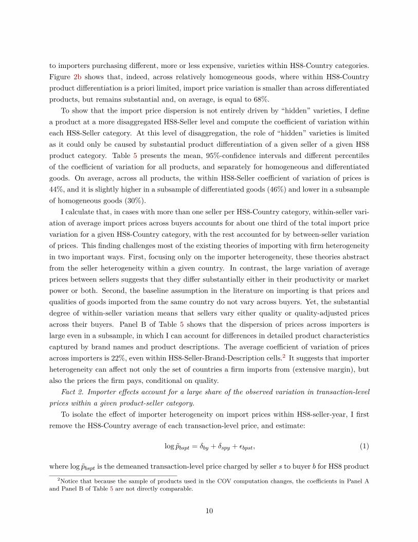
to importers purchasing different, more or less expensive, varieties within HS8-Country categories.Figure 2b shows that, indeed, across relatively homogeneous goods, where within HS8-Countryproduct differentiation is a priori limited, import price variation is smaller than across differentiatedproducts, but remains substantial and, on average, is equal to 68%.

To show that the import price dispersion is not entirely driven by “hidden” varieties, I definea product at a more disaggregated HS8-Seller level and compute the coefficient of variation withineach HS8-Seller category. At this level of disaggregation, the role of “hidden” varieties is limitedas it could only be caused by substantial product differentiation of a given seller of a given HS8product category. Table 5 presents the mean, 95%-confidence intervals and different percentilesof the coefficient of variation for all products, and separately for homogeneous and differentiatedgoods. On average, across all products, the within HS8-Seller coefficient of variation of prices is44%, and it is slightly higher in a subsample of differentiated goods (46%) and lower in a subsampleof homogeneous goods (30%).

I calculate that, in cases with more than one seller per HS8-Country category, within-seller vari-ation of average import prices across buyers accounts for about one third of the total import pricevariation for a given HS8-Country category, with the rest accounted for by between-seller variationof prices. This finding challenges most of the existing theories of importing with firm heterogeneityin two important ways. First, focusing only on the importer heterogeneity, these theories abstractfrom the seller heterogeneity within a given country. In contrast, the large variation of averageprices between sellers suggests that they differ substantially either in their productivity or marketpower or both. Second, the baseline assumption in the literature on importing is that prices andqualities of goods imported from the same country do not vary across buyers. Yet, the substantialdegree of within-seller variation means that sellers vary either quality or quality-adjusted pricesacross their buyers. Panel B of Table 5 shows that the dispersion of prices across importers islarge even in a subsample, in which I can account for differences in detailed product characteristicscaptured by brand names and product descriptions. The average coefficient of variation of pricesacross importers is 22%, even within HS8-Seller-Brand-Description cells.2 It suggests that importerheterogeneity can affect not only the set of countries a firm imports from (extensive margin), butalso the prices the firm pays, conditional on quality.

Fact 2. Importer effects account for a large share of the observed variation in transaction-levelprices within a given product-seller category.

To isolate the effect of importer heterogeneity on import prices within HS8-seller-year, I firstremove the HS8-Country average of each transaction-level price, and estimate:

log pbspt = δby + δspy + ϵbpst, (1)

where log pbspt is the demeaned transaction-level price charged by seller s to buyer b for HS8 product2Notice that because the sample of products used in the COV computation changes, the coefficients in Panel A

and Panel B of Table 5 are not directly comparable.

10

mean 95%-CI p10 p25 p50 p75 p90 count

Panel A: Within HS8-Seller

All products 0.44 [0.42, 0.45] 0.04 0.12 0.32 0.66 1.02 237 683

Differentiated 0.46 [0.44, 0.47] 0.05 0.15 0.36 0.68 1.04 202 712Homogeneous 0.30 [0.28, 0.33] 0.01 0.05 0.15 0.44 0.84 34 971

Panel B: Within HS-Seller-Brand-Description

All products 0.22 [0.20, 0.24] 0 0.02 0.11 0.29 0.61 65 879

Differentiated 0.24 [0.22, 0.27] 0.00 0.04 0.13 0.33 0.66 54 521Homogeneous 0.12 [0.10, 0.15] 0 0.00 0.03 0.14 0.33 11 358

Table 5: Coefficient of variation of import prices within HS8-Seller across buyers, 2013-2018.

p at time t; δby collects buyer-year fixed effects, and δspy collects seller-HS8-year fixed effects. Noticethat the seller-product-year fixed effects can be only estimated for a subsample of sellers that sellthe same HS8 product to at least two buyers in a given year. Analogously, buyer fixed effects areestimated based off a subsample of buyers that source at least two different HS8-Seller products ayear. These two conditions result in the loss of about a half of observations.

The results of estimation are presented in Table 6, which shows the percentage of the variationin (demeaned) transaction prices accounted for by buyer-year and seller-product-year fixed effects.First, both fixed effects account for a large share of within HS8-Country variation in import prices,as suggested by the adjusted R2 of 37%, on average across all products. Second, buyer-year fixedeffects across all products explain about 20% of the total variation of import prices within HS8-Country categories. This share is larger for homogeneous and consumption goods, where it reaches55% and 39%, respectively.

Cov(δby ,log p)V ar(log p)

Cov(δspy ,log p)V ar(log p) Adj. R2 N

All products 20.5% 79.5% 0.37 1 193 223

Homogeneous 54.5% 45.5% 0.41 187 834Differentiated 20% 80% 0.37 945 031

Consumption 38.5% 61.5% 0.37 294 293Intermediate 26.2% 73.8% 0.37 612 456

Table 6: Variance decomposition of transaction-level prices within HS8-Country, 2013 - 2018

11

Therefore, in contrast to the existing theories of importing, buyer heterogeneity accounts for asubstantial share of import price variation, even conditional on the buyer’s sourcing strategy definedat the disaggregated seller-HS8 level. The existing literature has provided only one explanation forthis empirical fact: due to complementaries between buyer productivity and seller quality, large,productive firms specialize in importing of higher-quality goods from a given supplier (Blaum et al.(2017)). In the next section, I argue that buyer productivity is systematically correlated withimport prices, even conditional on quality of imported goods.

3 Empirical Evidence of Price Discrimination

3.1 Main Results

Here I show that import prices systematically vary across importers of different size, conditional onthe quality of imported goods. The main challenge is that neither quality of imported goods, notfirm size are directly observed in the data. To overcome this problem, I explore the richness of mycustoms data and experiment with several different proxies for firm size and quality of importedgoods.

First, I consider quantity purchased within a given transaction as a measure of firm size, andinvestigate how it relates to the price charged by the seller. To capture differences in quality ofimported goods across buyers, I experiment with a large set of HS8-seller-year fixed effects andmore granular HS8-seller-brand-description fixed effects. Table 7 presents the results, where in allspecifications, I additionally include country-quarter fixed effects to absorb the differences in seller’scosts across time within a year. Columns (1) to (3) show that buyers purchasing larger volume of agiven HS8 product from a given seller pay lower per unit prices. A one percent increase in quantitywithin a transaction is associated with a 0.25% reduction in price.

If HS8-seller-year fixed effects do not fully absorb differences in quality, and if there are comple-mentaries between importer productivity and quality of imports, then this OLS estimate is expectedto be downward biased. To assess if this is true in the data, in column (2) I allow for homogeneousgoods, where quality differentiation is a priori limited to have a different slope coefficient, whichis expected to be larger in absolute value. The results suggest that buyers of relatively more ho-mogeneous products experience 0.06 percentage points larger reduction in per-unit price with theincrease in quantity.

In column (3), I investigate whether the relationship between prices and quantities are differentacross intermediate goods and final goods (which include consumption goods and capital goods).There could be several reasons for the relationship to be different across product types. First,consumer and capital goods could have more dimensions of product differentiations that are hardto describe, compared to intermediate inputs. Secondly, consumer and capital goods are likely tobe traded between wholesalers and retailers, which are usually multi-product firms that can sellvery different products even within HS8-seller categories. In contrast, intermediate goods are likely

12

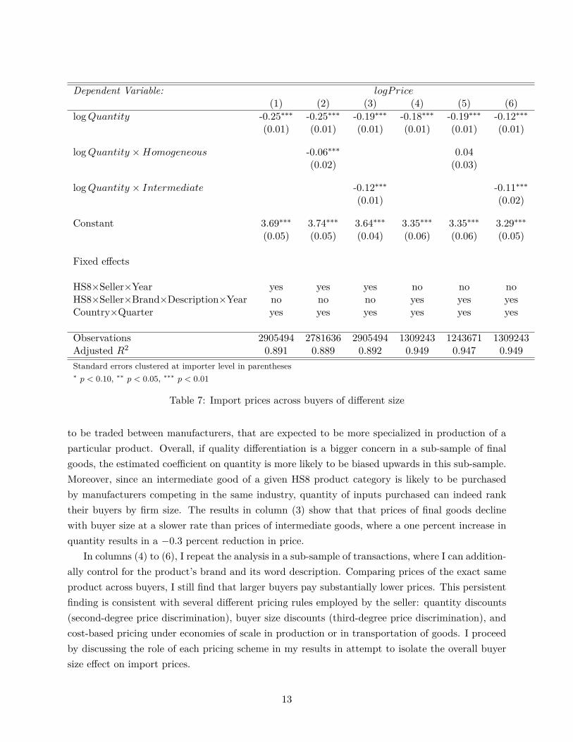
Dependent Variable: logPrice(1) (2) (3) (4) (5) (6)

logQuantity -0.25∗∗∗ -0.25∗∗∗ -0.19∗∗∗ -0.18∗∗∗ -0.19∗∗∗ -0.12∗∗∗(0.01) (0.01) (0.01) (0.01) (0.01) (0.01)

logQuantity ×Homogeneous -0.06∗∗∗ 0.04(0.02) (0.03)

logQuantity × Intermediate -0.12∗∗∗ -0.11∗∗∗(0.01) (0.02)

Constant 3.69∗∗∗ 3.74∗∗∗ 3.64∗∗∗ 3.35∗∗∗ 3.35∗∗∗ 3.29∗∗∗(0.05) (0.05) (0.04) (0.06) (0.06) (0.05)

Fixed effects

HS8×Seller×Year yes yes yes no no noHS8×Seller×Brand×Description×Year no no no yes yes yesCountry×Quarter yes yes yes yes yes yes

Observations 2905494 2781636 2905494 1309243 1243671 1309243Adjusted R2 0.891 0.889 0.892 0.949 0.947 0.949Standard errors clustered at importer level in parentheses∗ p < 0.10, ∗∗ p < 0.05, ∗∗∗ p < 0.01

Table 7: Import prices across buyers of different size

to be traded between manufacturers, that are expected to be more specialized in production of aparticular product. Overall, if quality differentiation is a bigger concern in a sub-sample of finalgoods, the estimated coefficient on quantity is more likely to be biased upwards in this sub-sample.Moreover, since an intermediate good of a given HS8 product category is likely to be purchasedby manufacturers competing in the same industry, quantity of inputs purchased can indeed ranktheir buyers by firm size. The results in column (3) show that that prices of final goods declinewith buyer size at a slower rate than prices of intermediate goods, where a one percent increase inquantity results in a −0.3 percent reduction in price.

In columns (4) to (6), I repeat the analysis in a sub-sample of transactions, where I can addition-ally control for the product’s brand and its word description. Comparing prices of the exact sameproduct across buyers, I still find that larger buyers pay substantially lower prices. This persistentfinding is consistent with several different pricing rules employed by the seller: quantity discounts(second-degree price discrimination), buyer size discounts (third-degree price discrimination), andcost-based pricing under economies of scale in production or in transportation of goods. I proceedby discussing the role of each pricing scheme in my results in attempt to isolate the overall buyersize effect on import prices.

13

Under second-degree price discrimination, the seller does not observe each buyer’s size and,to maximize profits, designs a non-linear pricing scheme that encourages the buyers to truthfullyreveal their type. Such non-linear pricing scheme are associated with quantity discounts: buyerwith larger orders are charge smaller per-unit mark-ups. On the other extreme, cost-based pricingunder economies of scale implies that sellers experience cost reductions on larger orders and fullypass along their cost savings to the buyers. Both of these pricing schemes imply that large volumebuyers pay lower per-unit prices, which could lead to the results reported in Table 7.

Separating these two effects from the buyer size effect, whereby buyers with different intrinsiccharacteristics pay different prices, is possible in a sub-sample of buyers with multiple orders fromthe same supplier per year. In Table, I estimate the relationship between per-unit price and totalyearly quantity of a given product using a sub-sample of buyers with multiple shipments of a givengood from a given seller per year. I find that a one percent increase in the overall quantity purchaseda year is associated with 0.09% decrease in a transaction-level price. In column (3), I additionallyinclude the quantity purchased at a time to control for second-degree price discrimination andeconomies of scale, and still find that buyers obtain additional discounts purely due to the size.Columns (4) and (5) show that the buyer-size discounts on top of the quantity discounts are largerin subsamples of homogeneous and intermediate goods. In these sub-samples, for a given volume ofa transaction, a one percent increase in the total yearly quantity purchased from the supplier, onaverage, is associated with 0.11% and 0.06% reduction in prices of homogeneous and intermediategoods, respectively.

The remaining concern with quantities transacted between a buyer and a supplier is that itmay not provide a truthful ranking of firms by their size. Firstly, if buyers of a given productbelong to different industries, they might have different production requirements causing quantitiesof imported goods to vary across buyers, irrespective of their true size. Secondly, if buyers belongto different industries, then differences in the demand for a given imported good can merely reflectdifferences in the demand of their output rather than firm productivity itself. To address thisproblem, it is necessary to control for the industry of the buyer, which is unavailable in customsdata. However, in a sub-sample of importers that also export their output, I can assign importersto the industry based on the products that they export. Specifically, I consider exporting importersthat export products belonging to the only HS2 product category and assign that product categoryas the importer’s main industry.

In Table 9, I repeat the analysis summarized in Tables 7 - 8 in sub-sample of exporting importersthat allows me to control for the industry of the buyer. In columns (1) and (2), I use the size ofa given shipment as a measure of buyer size and additionally control for the product-industry-yearfixed effects in column (2), relative to column (1). The results barely change with the inclusion ofindustry controls, which is in line with the quantity discounts interpretation of the price-quantityrelationship. Under second-degree price discrimination, the seller does not observe buyer’s identityor industry the buyer belongs to, and charged the price solely based on the volume of the order.

14

Dependent Variable: logPrice(1) (2) (3) (4) (5)

logQuantity -0.18∗∗∗ -0.18∗∗∗ -0.23∗∗∗ -0.14∗∗∗(0.01) (0.01) (0.01) (0.03)

log Y earlyQuantity -0.09∗∗∗ -0.03∗∗∗ -0.11∗∗∗ -0.06∗∗(0.02) (0.01) (0.02) (0.02)

Constant 3.29∗∗∗ 3.05∗∗∗ 3.53∗∗∗ 4.10∗∗∗ 2.57∗∗∗(0.06) (0.11) (0.11) (0.16) (0.29)

Fixed effects

HS8×Seller×Brand×Description×Year yes yes yes yes yesCountry×Quarter yes yes yes yes yesHomogeneous goods only no no no yes noIntermediate goods only no no no yes

Observations 1170020 1170020 1170020 573620 196342Adjusted R2 0.946 0.941 0.946 0.924 0.969Standard errors clustered at importer level in parentheses∗ p < 0.10, ∗∗ p < 0.05, ∗∗∗ p < 0.01

Table 8: Quantity discounts vs. Buyer size discounts

In contrast, when adding industry controls in column (4) relative to column (3), where buyersize is measures with yearly quantity of the good purchased, buyer-size discounts substantiallyincrease. Columns (5) and (6) show that buyer-size discounts, conditional on the volume in a giventransaction, are substantially larger in a sub-sample of exporting importers than in the full sample.Namely, conditional on the size of a given shipment, a one percent increase in the overall yearlyquantity purchased from a given seller results in 0.22% reduction in price, which is higher largerthan a 0.03% reduction estimated in the full sample of importers. Additionally controlling forthe buyer’s industry increases the magnitude of the buyer discount to 0.39% and barely changesquantity discounts.

15

Dependent Variable: logPrice(1) (2) (3) (4) (5) (6)

logQuantity -0.19∗∗∗ -0.18∗∗∗ -0.19∗∗∗ -0.17∗∗∗(0.03) (0.04) (0.03) (0.04)

log Y earlyQuantity -0.33∗∗∗ -0.53∗∗∗ -0.22∗∗ -0.39∗∗∗(0.12) (0.15) (0.11) (0.14)

Constant 3.47∗∗∗ 3.40∗∗∗ 4.88∗∗∗ 6.30∗∗∗ 4.98∗∗∗ 6.18∗∗∗(0.16) (0.18) (0.86) (1.08) (0.75) (0.96)

Fixed effects

HS8×Seller×Brand×Description×Year yes yes yes yes yes yesCountry×Quarter yes yes yes yes yesHS8×Country×Industry× Year no yes no yes no yes

Observations 140056 127106 140056 127106 140056 127106Adjusted R2 0.942 0.945 0.936 0.940 0.942 0.945Standard errors clustered at importer level in parentheses∗ p < 0.10, ∗∗ p < 0.05, ∗∗∗ p < 0.01

Table 9: Quantity discounts vs. Buyer size, Exporting Importers

4 Theoretical Framework

In this section, I develop a theoretical framework linking buyer’s productivity to the prices ofimported inputs she pays. The two main ingredients of this framework are strategic interactions oflarge intermediate goods producers and the endogenous choice of the extensive margin of sourcing.This framework predicts price discrimination in firm-to-firm transactions with large buyers of inputsobtaining better input prices. I further use the proposed framework to study the implications ofprice discrimination for consumer and producer gains from trade liberalization.

4.1 Environment

Consider the world consisting of N countries indexed by i and j. Each country i is populated byLi consumers that inelastically supply one unit of labor each and consume a continuum of finalgoods varieties. These varieties are produced by heterogeneous final goods producers, which differin their productivity ϕ. Production of final goods requires intermediate goods, which firms caneither produce themselves or purchase from independent input producers upstream. Final goodsproduction technology features increasing returns to scale with fixed costs depending on firm’sdecision to engage in in-house production of inputs. There is free entry in the final goods market,and the market structure is monopolistic competition.

16

Fixed number of intermediate goods producers in each country j produce substitutable inputsusing labor as the only input in their linear production function. They compete in prices and arelarge enough relative to the market to internalize the effects of their decisions on aggregate marketoutcomes. This departure from traditional international trade literature that assume atomisticfirms with no market power, brings several new insights. First, it implies that firms charge variablemark-ups of price over marginal costs: input producers with larger market share face lower perceivedelasticity of demand and thus can charge higher mark-ups. Second, market power allows same inputproducers to charge different prices to different buyers for the same good.

For third-degree price discrimination to arise in equilibrium, the following assumptions need tobe satisfied. Firstly, intermediate goods producers can observe individual characteristics of theirdownstream buyers, and, secondly, intermediate goods can only be purchased from their respectiveproducers (in other words, re-selling is not possible).

The sequence of moves in this environment is as follows. First, each potential entrant intothe final goods market pay entry costs in terms of labor and learn their productivity. Second,those firms that decide to stay on the market, consider investing additional fixed costs in inputsproduction technology and exporting. Third, intermediate goods producers decide what prices tocharge to their buyers downstream. And in the last stage, final goods producers make their inputsourcing and pricing decisions.

In the following sections I describe the details of the model and outline the industry equilibrium.

4.2 Preferences

Consumers in country i have identical preferences represented by the standard CES utility functionover a set Ωi of final goods’ varieties ω:

Ui = (

∫ω∈Ωi

qi(ω)σ−1σ dω)

σσ−1 (2)

These utility function gives rise to the following demand system in country i:

qi(ω) = EiPσ−1i pi(ω)

−σ,

where pi(ω) is the price of variety ω, Pi ≡( ∫

ω∈Ωipi(ω)

1−σidω) 1

1−σi is the standard CES price indexof final goods, and Ei is country i’s aggregate spending on manufacturing goods.

4.3 Technology and market structure

In this economy final goods are produced in the downstream sector, which relies on inputs suppliedby the upstream sector. Below I describe the market structures in both sectors.

Downstream sector. Each final goods variety is sold by a single firm in a monopolisticallycompetitive environment with free entry. Potential entrant f pays a sunk cost fe to draw a random

17

productivity ϕf and then choose whether to pay per-period fixed costs of production f . In everyperiod, there is an exogenous probability of exit, β.

Firms that stay in the market produce final goods using the following production function:

Yf = ϕf

(L

ζ−1ζ

f +Xζ−1ζ

f

) ζζ−1

(3)

Xf =((αDXD

f )ρ−1ρ + (αMXM

f )ρ−1ρ

) ρρ−1 (4)

where Yf is the output of downstream firm with productivity draw ϕf , using labor Lf , the domesticintermediate good XD

f and the aggregate imported intermediate good XMf . Parameters αD and

αM reflect the quality of domestic and imported inputs, respectively.The imported composite input XM

f is a CES aggregate over all foreign input suppliers of firmf . Apart from buying inputs from a common set of independent suppliers Ω, firm f can also payfixed costs of “backwards integration”, fBI , and produce inputs in-house at marginal costs pBI .Therefore, the imported composite input XM

f can be expressed as:

XMf =

(∑n∈Ω

(αnxnf )η−1η + 1f (α

BIxBIf )η−1η

) ηη−1

, (5)

where 1f is an indicator function, which is equal to one if firm f backwards integrate in the inputproduction.

There are at least two aspects of the downstream technology (3) - (5) worth emphasizing. First,the quality parameters αn do not vary across buyers of inputs. It means that there are inputproducers that sell exactly the same products to all downstream firms. Second, the average qualityof inputs varies across downstream firms only if there is selection into backwards integration. Inthis model, backwards integration is the only source of heterogeneity in the extensive margin ofinputs sourcing across firms. However, the model can be interpreted more broadly to encompassother explanations of the observed differences in the extensive margin of sourcing. If there aresearch costs of finding a supplier (as in Krolikowski and McCallum (2017), Bernard et al. (2015))or transaction costs of outsourcing (as in Kikuchi et al. (2012)), the term 1f (α

BIxBIf )η−1η will reflect

firm f ’s decision whether to incur those costs or not. Likewise, this term will capture firm’s decisionto incur relationship-specific investment to obtain a “better” quality (ie tailored) input from anycommon supplier.

Upstream sector. Unless produced in-house, all imported inputs in this economy can onlybe purchased from a fixed (exogenous) number of foreign producers, Ω. To produce one unit ofan input of quality αn, input producer n with productivity ψn uses labor, Ln, according to theCobb-Douglas technology:

αn = (Lnψn)θ, (6)

18

where 0 < θ < 1 reflects diminishing returns to quality.Input producer n faces iceberg trade costs τn > 1 and chooses the free on board (f.o.b) price

pkn for each buyer k. In doing so, firms supplying the same buyer compete oligopolistically, andinternalize the effect of their pricing decisions on buyer’s costs of sourcing inputs. Therefore, whenquoting a price to its buyer, the firm takes into account the possibility of backwards integrationinto the input production by the buyer.

After downstream producers pay the fixed costs of entry and learn their productivity, the gameproceeds in three stages: first, the upstream firms choose the prices of inputs, pkn k, then thedownstream firms decide whether to backwards integrate or not, and in the final stage productiondecisions are made.

In the next subsection, I describe the problems of both upstream and downstream firms and showhow oligopolistic competition in the upstream sector combined with the possibility of backwardsintegration in the downstream sector results in price discrimination in the inputs market.

4.4 Firms’ objective functions and equilibrium input prices

In the final stage of the game, each downstream firm f chooses price pf to maximize its profits:

maxpf

(pf − cf )p−σf EP σ−1 − fw − 1ffBIw, (7)

where the marginal costs of the firm cf is the unit-cost function dual to the production function in(3):

cf ≡ 1

ϕf

(w1−ζ + P 1−ζ

f

) 11−ζ (8)

Monopolistic competition in the downstream sector implies that the solution to (7) is a constantmark-up over firm f ′s marginal costs:

pf =σ

σ − 1cf (9)

If firm f stays on the markets, its output, revenue and total profits will be given by:

qf = c−σf EP σ−1m−σ (10)

rf = c1−σf E(P/m)σ−1 (11)

πf =rfσ

− fw − 1ffBIw (12)

where m ≡ σσ−1 denotes a constant mark-up, common across all downstream firms.

In the second stage, the downstream firms must decide whether to backwards integrate intothe input production or not, given the prices of independent suppliers. As can be see from (5),backwards integration reduces the costs of sourcing inputs from abroad through the “love-of-variety”

19

effect of the CES production function. Specifically, the unit-cost function dual to (5) is given by:

PMf =

(∑n∈Ω

(pnf/αnf )

1−η + 1f (pBI/αBI)1−η

) 11−η

(13)

On the other hand, it is associated with higher fixed costs of production. Backwards integrationoccurs when the benefits from backwards integration outweigh the costs. Suppose that the firm’sdecision represented by 1f can be approximated with a continuous function ∆. Then taking thederivative of πf with respect to ∆ and letting ∆ → 0 yields:

∂πf∂∆

|∆→0 =1

η − 1c−σf EP σ−1m−σ︸ ︷︷ ︸

=qf

cfsBI − fBIw =1

η − 1qfcfsBI − fBIw (14)

where sBI ≡ pBIxBI

wL+∑n∈Ω

pnxnis a share of the in-house produced input in total production costs when

∆ → 0. This share is large when the quality-adjusted price of the firm’s own input is low relativeto the average quality-adjusted prices of the inputs the firms buys. From (14), it follows thatbackwards integration is profitable when

1

η − 1cfsBI >

fBIw

qf, (15)

where the left-hand side represents the per-unit costs savings due to backwards integration, and theright-hand side is the costs of backwards integration per unit of output. Note that when productsare perfect substitutes (η → ∞), there is no “love-of-variety” effect, which leads to zero costssavings from backwards integration.

Condition (14) also implies that a firm has to be large enough in terms of its output qf for back-wards integration to become profitable. Specifically, there is a productivity cut-off for backwardsintegration, ϕBI , such that only firms with productivity draw above it backwards integrate:

ϕBI =

(fBIw(η − 1)

EP σ−1m−σsBI

) 1σ−1

c, (16)

where c ≡(w1−ζ + P 1−ζ) 1

1−ζ is a cost index under no backwards integration, common across alldownstream firms.

Proposition 1. There exist a productivity cut-off, ϕBI , such that only downstream firms withproductivity draws above the cut-off, backwards integrate into the production of inputs. Thisproductivity cut-off is determined in expression (16).

Proof follows from the profit maximizing condition with respect to backwards integration in(14).

In the first stage, the input producers upstream choose input prices for the downstream firms

20

to maximize profits. Since there are two types of input buyers - those that backwards integrateand those that do not - price discrimination is profit maximizing. Thus, upstream producer nmay choose different prices to different buyers as a solution to the following profit maximizationproblem:

maxpnf

(pnf −

wn (αn)1/θ τn

ψn

)αM

ρ−1αn

η−1

(pnf

PMf

)−η (PMfPf

)−ρ

Xf︸ ︷︷ ︸=demand for input xnf

(17)

As a solution to this profit maximization problem, the upstream producer will choose price pnf ,according to the Lerner index:

pnf −1ψnwn (αn)

1/θ τn

pnf=

1

εnf(18)

where the left-hand side is a mark-up over the upstream producer’s costs and the right-hand sideis the inverse of demand elasticity of the downstream buyer of input n. This elasticity can beexpressed as a function of supplier n in firm f ’s expenditures on imported inputs, snf :

εnf ≡ −∂xnf∂pnf

pnfxnf

= η − (η − ρ)snf , (19)

where snf ≡ (pnf /αn)1−η

(PMf )1−η is the share of input n in firm f ’s expenditures on imported inputs.

The downstream firms that can backwards integrate (those with ϕf exceeding ϕBI) spend asmaller share of their expenditures on each common across firms producer n. It means that due tobackwards integration, larger downstream firms have larger demand elasticity for any input theypurchase.

The profit maximizing condition in (18) suggests that the input price can be decomposed intoa cost and a mark-ups components as follows:

pnf =εnf

εnf − 1︸ ︷︷ ︸mark-up

1

ψnwn (αn)

1/θ τn︸ ︷︷ ︸marginal costs

(20)

The input producers selling higher quality inputs charge higher prices to all their buyers, becausethey have both higher marginal costs of production and higher mark-ups. When comparing twodownstream buyers of one seller of the exact same quality input, larger buyers that backwardsintegrate into the input production obtain more favorable input prices because of the lower mark-ups. I summarize these results in the following proposition.

Proposition 2. Oligopolistic input producers producing higher quality inputs charge highermark-ups. For an input of the same quality, an oligopolistic input producer charges a higher mark-up to a buyer that does not backwards integrate and a lower mark-up to a buyer of the same quality

21

input that does backwards integrate.Proof follows from expressions in (18) - (20).Propositions 1 and 2 together suggest that the oligopolistic input producers engage in price dis-

crimination, such that, compared to their less productive rivals, more productive firms downstreamobtain better input prices for the exact same goods. In the next subsection, I explore what thedeviation from the Law of One Price implies for the industry equilibrium in the downstream sector.

4.5 The effect of price discrimination on the industry equilibrium

In the zero stage of the game, downstream firms decide whether they should stay on the marketor not after learning their productivity. The firm entry/exit decision pins down the industryequilibrium outcomes such as the number of active firms on the market, their average profits andthe consumer price index. In this subsection, I show that by improving intra-industry resourcereallocation, price discrimination in the inputs markets benefits final goods consumers throughlower prices.

Free entry requires that the sunk entry cost few equals the present value of expected profits:

few = (1−G(ϕ∗))1

βπ, (21)

where ϕ∗ is the exit productivity cut-off, 1 − G(ϕ∗) is the share of potential entrants that stayactive on the market after learning their productivity, π is the expected per-period profits of activefirms, and β is an exogenous probability of exit.

The least productive firm that stays on the market after learning its productivity earns zeroprofits. Assuming that this firm can not backwards integrate into the production of inputs, itsproductivity, ϕ∗, is determined from the zero-profit condition:

ϕ∗ =

(fw(σ − 1)

EP σ−1m−σ

) 1σ

c (22)

The expected per-period profits of active firms can be calculated as the profit of the firm withaverage productivity, c:

π =1

σc1−σE(P/m)σ−1 − fw − 1−G(ϕBI)

1−G(ϕ∗)fBIw (23)

where 1−G(ϕBI)1−G(ϕ∗)

is the probability of backwards integration.For the ease of derivations, I will further rely on the assumption that firm productivity in

the downstream sector, G(ϕ) has a Pareto distribution with the shape parameter κ: G(ϕ) =

1 − ϕ−κ. Then using the expressions for productivity cut-offs (16) and (22) in (23), one can findthe equilibrium average profits:

22

π =σ − 1

κ− σ + 1fwΛ, (24)

where Λ ≡ 1 +(fBIf

)σ−κ−1σ−1

(γ − 1)κ

σ−1 is increasing in the extend of price discrimination γ. Notethat the Law of One Price implies that γ = 1 and thus underestimates the average profits inthe downstream sector. In contrast, the larger is the extend of price discrimination, the higherper-period average profits.

Since in equilibrium more productive firms downstream obtain better input prices, price dis-crimination improves the intra-industry allocation of resources, leading to higher average profits.The reallocation of resources from less to more productive firms, however, comes at the cost ofhigher exit rates under price discrimination. Using the expression for the expected profits in thefree entry condition (21), one can find that the exit productivity cut-off increases in the extend ofprice discrimination:

ϕ∗ =

(σ − 1

κ− σ + 1

f

feβΛ

) 1κ

(25)

As a result, price discrimination in the inputs markets implies higher market concentration inthe downstream sector. In equilibrium, the number of active firms downstream is given by

M = 1−G(ϕ∗) =κ− σ + 1

σ − 1

βfeΛf

(26)

Since price discrimination results in higher average productivity and does not change firms’ marketpower (mark-ups are constant with the CES preferences), it is expected to increase consumer welfarethrough lower prices. To derive this result formally, I use the zero-profit condition for the leastproductive active firm, ϕ∗ to derive the price index faced by final consumers:

P =

(σ − 1

κ− σ + 1

f

βfeΛ

)− 1κ(fσ

E

) 1σ−1

mc (27)

It is easy to see that the extend of price discrimination reduces the final goods price index, thusbenefiting the consumers. In the next proposition I summarize the effects of price discriminationin the inputs market on the industry equilibrium.

Proposition 3. Deviation from the Law of One Price in the form of price discrimination in theinputs markets implies higher average profits, higher market concentration, and lower final goodsprices.

Proof follows from the expressions in (23), (26), (27) and the fact that Λ increases in the extendof price discrimination.

23

5 Price Discrimination and the Gains from Trade

5.1 Input trade liberalization

I use the framework introduced above to understand the mechanisms through which trade reformsaffect firm performance and social welfare. Since firms participate in international markets asboth buyers of inputs and sellers of final goods, they are affected by both input and output tradeliberalization reforms. In this paper, I explore how the deviation from the Law of One Priceaffects welfare gains from both types of reforms. In this subsection, I focus on the effect of pricediscrimination on welfare gains from input trade liberalization.

The proposed theoretical framework allows for three mechanisms through which a reduction ininput tariffs can affect firm performance in the downstream sector: the intensive and the extensivemargins of trade in inputs and the intra-industry reallocation of activities across downstream firms.In what follows, I study each mechanism separately.

As it was derived above, in equilibrium, the price of input n faced by firm f can be written asa firm-specific mark-up times marginal costs:

pnf = µnf (pnf )cn, (28)

where µnf (pnf ) ≡εnf (p

nf )

εnf (pnf )−1 is a function of the input demand elasticity, which depends on input n’s

share in firm f ’s expenditures. Since this share itself depends on the price of the input, it followsthat both the input demand elasticity and the mark-up can be written as function of pnf .

Now consider a reduction in tariffs faced by input producer n, equivalent to the reduction iniceberg trade costs τn. To understand the cost-shock pass-through into the input price, rewriteequation (28) in logs:

logpnf = logµnf (pnf ) + logcn (29)

Denoting the mark-up elasticity with respect to price with Γnf = −dlogµnf (p

nf )

dlogpnfand taking first

differences of (29) yields:dlogpnf = −Γnfdlogp

nf + dlogτn (30)

From here it follows that the change in the input price due to the input trade liberalization isdetermined by the mark-up elasticity with respect to price:

dlogpnfdτn

=1

1 + Γnf(31)

Note that if Γnf is positive, then the pass-through is incomplete, and it decreases with Γnf . Intuitively,a reduction in tariffs leads to an increase in firm’s market share, which induces the firms to increasethe mark-ups. As a result, the buyers of inputs benefit through a less than complete pass-throughof the full cost reduction.

24

Given the input demand elasticity in (??), the mark-up elasticity with respect to price becomes

Γnf =(η − ρ)(η − 1)snf

(1− snf

)εnf

(εnf − 1

) > 0 (32)

It is positive and increases in the input’s expenditure share for inputs with less than 50% sharein firms’ total expenditures. Hence, larger downstream buyers that backwards integrate enjoylarger cost-shock pass-through. In other words, larger buyers downstream gain more from inputtrade liberalization than smaller ones. The same result holds if the cost shock originates from theexchange rate volatility.

Importantly, the cost-shock pass-through is incomplete and decreases in the buyer’s size solelydue to the mark-ups being variable across the buyers of inputs. If sellers of inputs charged thesame mark-up to all their buyers, the cost-shock pass-through would be the same across the buyers.Therefore, if, given the same cost shock, larger buyers experience larger price changes in the data,it in itself proves the existence of price discrimination. This result is summarized in the followingproposition.

Proposition 4. If input producers compete oligopolistically and can price discriminate, thecost-shock pass-through is incomplete and heterogeneous across input buyers. Specifically, thecost-shock pass-through (weakly) decreases in the buyer’s size.

Proof. The incompleteness of the cost-shock pass-through follows from (31). To see, how thepass-through relates to the buyer’s size, consider the expression for mark-up elasticity in (32).If snf ∈ [0, 1/2], it increases in input n’s share snf . Since larger buyers of inputs can backwardsintegrate, snf weakly decreases in buyer’s size. Hence, larger buyers of inputs experience largercost-shock pass-through.

5.2 Trade Liberalization Downstream

Now I relax the assumption that only intermediate goods are traded internationally and allow forexports of final goods. I introduce the following notation: subscript d denotes domestic economy,while subscript i denotes any foreign country.

Exporting final goods to any foreign country i requires investing fx fixed costs. Then, down-stream firms decide whether to export and backwards integrate by comparing the total profits ofthe four possible options, described below.

Profits if only serving the domestic market and outsourcing all inputs:

πOd =1

σEd(Pd/m)σ−1

(CO)1−σ

ϕσ−1 − f (33)

25

Profits if only serving the domestic market with in-house production of inputs:

πBId =1

σEd(Pd/m)σ−1

(CBI

)1−σϕσ−1 − nf (34)

Profits if exporting to country i and outsourcing all inputs:

πOx =1

σ

(CO)1−σ

ϕσ−1(Ed(Pd/m)σ−1 + τ1−σdi Ei(Pi/m)σ−1

)− f − fx (35)

Profits if exporting to country i with in-house production of inputs:

πBIx =1

σ

(CBI

)1−σϕσ−1

(Ed(Pd/m)σ−1 + τ1−σdi Ei(Pi/m)σ−1

)− nf − fx (36)

Exporting decision as well as the choice of a sourcing strategy S = BI,O are illustrated inFigure 3, where the four profit functions are plotted against firm productivity ϕ.

In equilibrium depicted in Figure 3, downstream firms self-select into four groups: the leastproductive firms (ϕσ−1 < ϕσ−1

∗ ) exit the market, the low productivity firms (ϕσ−1∗ ≤ ϕσ−1 ≤

ϕσ−1x ) outsource all their inputs and only serve the domestic final goods consumers, the medium

productivity firms (ϕσ−1x ≤ ϕσ−1 ≤ ϕσ−1

I ) still outsource all their inputs but also export their finalgoods, and finally, the most productive firms (ϕσ−1 > ϕσ−1

I ) both export and produce some of theirinputs in-house.

Note that in Figure 3, the parameters are such that the strategy of serving only domesticconsumers and producing some inputs in-house is always dominated by other strategies.It impliesthat there are no firms that invest in in-house production of inputs and do not export, which reflectsthe complementarity between exporting and in-house production.

In equilibrium, the demand for input k by downstream firms that outsource their inputs andby those that backwards integrate is, respectively:

xOk =

(pOk /δk

POf

)−η (POf /αf

POx

)−ρ (CO)−σ

(ϕ/m)σ(EdP

σ−1d + 1xτ

−σdi EiP

σ−1i

)xBIk =

(pBIk /δk

PBIf

)−η (PBIf /αf

PBIx

)−ρ (CBI

)−σ(ϕ/m)σ

(EdP

σ−1d + τ−σdi EiP

σ−1i

),

(37)

where 1x is an indicator function, which is equal to one if the firm is an exporter and zerootherwise.

To study how trade liberalization (i.e. reduction in bilateral iceberg trade costs τdi ) affects firms’incentives to backwards integrate and export, it is useful to write down the cut-off productivities,ϕ∗, ϕx and ϕI .

26

Figure 3: Exporting and Input sourcing modes

The exit productivity cut-off ϕ∗ is determined from the zero-profit condition:

πOd (ϕ∗) = 0 ⇔ 1

σEd(Pd/m)σ−1

(CO)1−σ

ϕσ−1∗ − f = 0 (38)

Since the marginal exporter from d to i outsources all its inputs, the exporting productivitycut-off ϕx can be expressed as a function of ϕ∗ using πOd (ϕx) = πOx (ϕx) as:

ϕx = ϕ∗

(fx/(EiP

σ−1i )

f/(EdPσ−1d )

) 1σ−1

τdi (39)

Hence, as long as fx/(EiPσ−1i )

f/(EdPσ−1d )

> 1, ϕx > ϕ∗, as illustrated in Figure 3.Finally, the least productive firm that can produce inputs in-house is an exporter. The produc-

tivity of this firm, ϕI , is found from πBIx (ϕI) = πOx (ϕI) as:

ϕI = ϕ∗

(n− 1

γ − 1

EdPσ−1d

EdPσ−1d + τ1−σdi EiP

σ−1i

) 1σ−1

(40)

From the expressions (39) - (40) it follows that both exporting and backward integration pro-ductivity cut-offs are increasing in iceberg trade costs τdi. In other words, the reduction in trade

27

costs due to trade liberalization with country i allows firms that previously did not export to startexporting. Moreover, some firms that found it profitable to export even before trade liberalization,now find it also profitable to invest in the upstream technology. This is because trade liberalizationworks as a (arguably exogenous) shock to the demand for goods produced by exporters, whichmakes backward integration more profitable.

The described effects of trade liberalization in the downstream sector are illustrated in Figure 4.

Figure 4: The effects of trade liberalization

Figure 4 makes it clear that gains from trade liberalization are heterogeneous across differentdownstream firms. For example, firms that were large exporters of final goods even before tradeliberalization are not expected to gain through lower input prices, as they already obtain low inputprices due to their size. On the other hand, very small domestic producers of final goods still cannot export even after the decrease in transportation costs. It is only the more productive newexporters and less productive old exporters that are predicted to gain through lower input prices.After the reduction in trade costs, those firms experience a positive demand shock, which makesin-house production of inputs more profitable and allows them to obtain lower input prices fromthe upstream producers.

Being positively correlated with firm sales, reductions in tariffs on final goods can be used asan instrumental variable for firm size when studying its effect on input prices faced by final goodsproducers.

In what follows I explore the implications of third-degree price discrimination in inputs marketsfor the downstream industry equilibrium.

5.3 Industry Equilibrium

Downstream industry equilibrium in country d consists of the price of final goods (Pd), (endogenous)number of firms (Md) and the average profits of active firms.

28

Free entry to the downstream sector requires that the sunk entry cost fe equals the presentvalue of expected profits:

fe = (1−G(ϕ∗))1

βπ, (41)

where 1−G(ϕ∗) is the share of potential entrant that stay active after learning their productivity,and π is an expected per-period profits of active firms. The expected per-period profits can beexpressed as the sum of expected profits from domestic sales and expected profits from exporting:

π = πd + pxπx, (42)

where px = 1−G(ϕx)1−G(ϕ∗)

is the share of exporting firms in the downstream sector. For the ease ofderivations, I will further assume that G(ϕ) is a Pareto cummulative distribution function with theshape parameter κ3:

G(ϕ) = 1− ϕ−κ

Under this distributional assumption, the expected profits become4:

π =σ − 1

κ− σ + 1f∆ (43)

∆ = 1+(fxf

)−κ+σ−1σ−1

(AdAi

)− κσ−1

τ−κ + (γ − 1)κ

σ−1 (n− 1)σ−κ−1σ−1

(Ad

Ad+τ1−σdi Ai

)−κ−σ−1σ−1

(1 + κσ−1

Aiτ−κ

fxAd),

where Aj = Ej(Pj/m)σ−1.As ∆ is increasing in the marginal cost advantage of in-house production γ, so is the average

profits in the downstream sector.Using the solution for expected profits (43) in the free entry condition (41), one can find the

exit productivity cut-off as a function of parameters, including ∆:

ϕ∗ =

(σ − 1

κ− σ + 1

f

βfe∆

) 1κ

(44)

This cut-off allows to solve for the number of active firms in the downstream sector of countryd:

Md = 1−G(ϕ∗) =κ− σ + 1

σ − 1

βfe∆f

(45)

Therefore, larger cost reductions due to in-house production implies fewer firms in the downstreamsector in equilibrium. This is because price discrimination in inputs markets leads to higher ex-pected profits in the downstream sector. Under free entry and constant mark-ups, higher expectedprofits can only be sustained with fewer firms on the market, hence - smaller Md.

3Standard assumption that found empirical support in international trade literature4For expected profits to be positive, the following restriction on the parameters should be satisfied: κ > σ − 1

29

Two other important productivity cut-offs, ϕx and ϕI can be easily obtained from (39) and (40):

ϕx =

(σ − 1

κ− σ + 1

f

βfe∆

) 1κ

(fx/τ

1−σdi Ai

f/Ad

) 1σ−1

τdi (46)

ϕI =

(σ − 1

κ− σ + 1

f

βfe∆

) 1κ

(n− 1

γ − 1

Ad

Ad + τ1−σdi Ai

) 1σ−1

(47)

Finally, the price index in the downstream sector can be solved for using the solution for ϕ∗and the zero-profit condition for the least productive active firm on the market (38):

Pd =

(σ − 1

κ− σ + 1

f

βfe∆

)− 1κ(fσ

Ed

) 1σ−1

mPOx (48)

Thus, final goods consumers gain from price discrimination, as it reduces the price of theconsumer goods: as γ increases, the final goods price index Pd falls.

30

6 Conclusion

The existence of price discrimination has been long documented and studied in industrial orga-nization, yet the international trade literature neglects the possibility of different firms gettingdifferent price for exact same product. I this paper, using firm-level Customs data, I showed thatthe assumption of common prices does not seem to hold in the data. When purchasing the sameinput, buyers with larger quantities obtain lower input prices. To rationalize this observation, Ibuild a model of trade in intermediate goods, in which there are differences in endogenous demandelasticity across buyers of inputs. In this model, heterogeneous downstream firms can decide toproduce inputs in-house and export their goods. Both exporting and in-house production are as-sociated with larger fixed costs. As a result, only initially more productive firms sort into in-houseproduction of inputs and exporting. As more productive firms can substitute inputs produced in-house for the one they buy from upstream suppliers, their demand on inputs is more elastic. Sinceinput prices are inversely proportional to the demand elasticity, upstream suppliers charge lowerprices to larger (more productive) downstream firms.

Incorporating price discrimination into the general equilibrium trade model allows to studyits implications for market aggregates. For instance, wider possibility for price discriminationin the upstream sector increases the expected profit of the downstream sectors and reduces thenumber of active firms in that sector. This, in turn, implies that consumers benefit from pricediscrimination through lower production costs of the final goods producers as well as the selectionof more productive firms.

This paper also showed that firms decisions to export and engage in in-house production ofinputs are complementary. On the one hand, by reducing firm’s production costs and thus increas-ing operational profits, in-house production of inputs allows firms to overcome the fixed costs ofexporting. On the other hand, by offering larger economies of scale, exporting itself encouragesfirms to set-up the production of inputs. Thus, instances of trade liberalization in the downstreamsectors can be used as exogenous shocks to identify the causal effect of firm’s productivity of theprices of inputs it faces.

The proposed framework with price discrimination in the inputs markets can be further used toempirically study the role of imported intermediates in firms productivity. When firms face differentprices on same inputs, it results in heterogeneity in productivity gains from trade liberalization inthe upstream sectors.

31

References

Antras, P., Fort, T. C., and Tintelnot, F. (2017). The margins of global sourcing: theory andevidence from us firms. American Economic Review, 107(9):2514–64.

Bernard, A. B., Jensen, J. B., and Schott, P. K. (2009). Importers, exporters and multinationals:a portrait of firms in the us that trade goods. In Producer dynamics: New evidence from microdata, pages 513–552. University of Chicago Press.

Bernard, A. B., Moxnes, A., and Saito, Y. U. (2015). Production networks, geography and firmperformance. Technical report, National Bureau of Economic Research.

Blaum, J., Lelarge, C., and Peters, M. (2017). Firm size and the intensive margin of import demand.

Chandra, A. and Lederman, M. (2015). Revisiting the relationship between competition and pricediscrimination in the airline industry. Rotman School of Management Working Paper, (2477719).

Feenstra, R. C. (1994). New product varieties and the measurement of international prices. TheAmerican Economic Review, pages 157–177.

Gerardi, K. S. and Shapiro, A. H. (2009). Does competition reduce price dispersion? new evidencefrom the airline industry. Journal of Political Economy, 117(1):1–37.

Javorcik, B. S. and Narciso, G. (2008). Differentiated products and evasion of import tariffs. Journalof International Economics, 76(2):208–222.

Jung, J. W., Simonovska, I., and Weinberger, A. (2015). Exporter heterogeneity and price discrim-ination: a quantitative view. Technical report, National Bureau of Economic Research.

Katz, M. L. (1987). The welfare effects of third-degree price discrimination in intermediate goodmarkets. The American Economic Review, pages 154–167.

Kikuchi, T., Nishimura, K., and Stachurski, J. (2012). Coase meets tarski: new insights fromcoase’s theory of the firm.

Krolikowski, P. M. and McCallum, A. H. (2017). Goods-market frictions and international trade.

Mishra, P., Subramanian, A., and Topalova, P. (2008). Tariffs, enforcement, and customs evasion:Evidence from india. Journal of public Economics, 92(10-11):1907–1925.

Rauch, J. E. (1999). Networks versus markets in international trade. Journal of internationalEconomics, 48(1):7–35.

Simonovska, I. (2015). Income differences and prices of tradables: Insights from an online retailer.The Review of Economic Studies, 82(4):1612–1656.

32