Butterfly Valve and Flow

8/3/2019 Butterfly Valve and Flow

http://slidepdf.com/reader/full/butterfly-valve-and-flow 1/5

NUMERICAL ANALYSIS OF BUTTERFLY VALVE-PREDICTION OF FLOW

COEFFICIENT AND HYDRODYNAMIC TORQUE COEFFICIENT

Xue guan Song1

, Young Chul Park 2

1Graduate student, [email protected]

2Professior, [email protected]

CAE Lab, Department of Mechanical Engineering, Dong-A University,

840 Hadan-dong, Saha-gu, Busan 604-714TEL: (82)051-200-6991; FAX: (82)051-200-7652

South Korea

ABSTRACTButterfly valves are commonly used as control

equipments in applications where the pressure drops

required of the valves are relatively low. As shutoff valve

(on/off service) or throttling valves (for flow or pressurecontrol), the higher performance and the better precision

of butterfly valves are required. Thus it’s more and more

essential to know the flow characteristic around the valve.

Due to the fast progress of the flow visualization and

numerical technique, it becomes possible to observe theflows around a valve and to estimate the performance of a

valve. In this paper, three-dimensional numerical

simulations by commercial code CFX were conducted toobserve the flow patterns and to measure valve flow

coefficient and hydrodynamic torque coefficient when

butterfly valve with various opening degrees and uniformincoming velocity were used in a piping system. By

contrast, a group of experimental data is used to compare

with the data obtained by CFX simulation to investigatethe validity of numerical method. Researching these

results did not gave only access to understand the process

of the valve flows at different valve opening degrees, butalso was made to determine the accuracy of the employed

method. Furthermore, the results of the three-dimensional

analysis can be used in the design of butterfly valve in the

industry.

KEY WORDS

butterfly valve, numerical simulation, flow coefficient,

hydrodynamic torque coefficient

1. IntroductionA butterfly valve (Fig. 1) is a type of flow control

device that controls the flow of gas or liquid in a variety

of process. It consists of a metal circular disc with its

pivot axes at right angles to the direction of flow in the pipe, which when rotated on a shaft, seals against seats in

the valve body. This valve offers a rotary stem movement

of 90 degrees or less in a compact design.The importance of butterfly valves has been more and

more increasing in the pipe system. And there are so

many reports on the characteristics, i.e. the flowcoefficient, the torque coefficient, the pressure recovery

factor and so on. Kerh et al. [1] performed an analysis of

the butterfly valve on the basis of the experimentalresults. Sarpkara [2] theoretically treated the

characteristics of a flat butterfly valve. Kimura and

Tanaka [3] studied the pressure loss characteristics

theoretically for a practical butterfly valve and so on.With the development of the Computational Fluid

Dynamics (CFD), the approach of using the technique of

computational fluid dynamics has been substantiallyappreciated in mainstream scientific research and in

industrial engineering communities. By now, the CFD

simulation by commercial code has been proved itsfeasibility to predict the flow characteristic. There have

been also many reports on valve using Computational

Fluid Dynamics analysis. Huang and Kim [4] performed a

three-dimensional numerical flow visualization of incompressible flows around the butterfly valve which

revealed velocity field, pressure distributions by using

commercial programs. Lin and Schohl [5] performed an

analysis about the application of CFD commercial package in the butterfly valve field. Chern and Wang [6]

employed a commercial package, STAR-CDTM, toinvestigate fluid flows through a ball valve and to

estimate relevant coefficient of a ball valve.

The main object of this research is to develop a model by using the commercial code ANSYS CFX 10.0, which

accurately represents the flow behaviour and provide a

three-dimensionalnumerical simulation

of water around the

butterfly valve and

estimate the pressure

drop, flow coefficientand hydrodynamictorque coefficient. It

is the first step

towards improvingvalve design. Fig. 1 Butterfly valve (D=1.8m)

Proceedings of the World Congress on Engineering and Computer Science 2007WCECS 2007, October 24-26, 2007, San Francisco, USA

ISBN:978-988-98671-6-4 WCECS 2007



stressesReynoldstheis jiuu ′′∂

2

1

j

i

j

ji

i

j

j

i j

x

uv

x

uu

x

pg

x

uu

∂

∂+

∂

′′∂−

∂

∂−=

∂

∂

ρ

2. Flow and hydrodynamic flow coefficient2.1 Flow coefficient C V

The flow coefficient is used to relate to the pressureloss of a valve to the discharge of the valve at a giving

valve opening angle. Today, C V is the most widely used

value for valve size and pipe system. By using the C V , a proper valve size can be accurately determined for most

applications. The most common form used by valve

industry is Equation (1):

where the pressure drop Δ P ISA can be measured from

static wall taps located 2 pipe diameters upstream and 6

pipe diameters downstream of the valve. And Δ P is the

pressure drop in units of psi, Qgpm is in units of gpm, and

Sg is the specific gravity of the fluid (1 for water ). In fact, this Equation ignored the affecting of friction

force. According to ISA testing specifications, it isnoticed that at valve of Cv/d 2 greater than 20, the affectingof the friction is significant and must be considered. In

terms of practical experience and evaluation in advance,most water valves, including this object, have value of Cv/d 2 greater than 20. Hence another Equation about

pressure drop with the fiction factor can be derived as

Equation (2):

where f is the friction factor, d is the diameter of valve

in units of inches.

So, the corrected Equation of C V can be written as

Equation (3):

2

2008986.0/ ⎟

⎠

⎞⎜⎝

⎛ ⋅⋅−Δ

=

d

Q f SP

QCv

g ISA

net

*Notice: Cv is a dimensional value.

2.2 Dynamic flow coefficient Ct

Hydrodynamic torque T( α) is the valve shaft produced

by the flow passing through the valve at a given valve

opening angle α. The hydrodynamic torque coefficient Ct

is a factor, which is independent of the size of the valve.For a given valve and valve opening, it is easy to calculate

the hydrodynamic flow torque by using Ct times the

different pressure drop, Equation (4) shows the relation between Ct , T , pressure drop and valve diameter.

3. CFD Model3.1 Model description

The prototype size is 1.8 m in diameter and it is

manufactured from cast steel with machined inside

surfaces. For getting a better result in this simulation, The

CFD model of butterfly valve is created at a 1:1 scalewith a rough (roughness height estimated to be about 0.5

mm) inside surface. It has a shape similar to “Discus” and

its maximum thickness in the middle of the valve is 360

mm and the minimum along the flange is 20 mm. Theupstream length L1 and downstream length L2 are addedto provide a flow field.

3.2 Flow Pattern

The fluid, which was modeled as water, is given auniform velocity of 3m/s at the inlet and zero reference

pressure at the outlet.

Through rough calculation, the range of Reynolds

Number of flow in this study is larger than 105, hence the

effect of the Reynolds Number is so small that it can be

neglected [7].

3.3 Numerical Method

Incompressible and viscous fluid (water) flows throughthe butterfly valve. The flow pattern reveals that the flow

studied is turbulence flow.

To deal with the turbulence modeling, the eldest

approach, Reynolds-averaged Navier-Stokes Equations

(RANS), is utilized. Its common form can be written asEquation (5)

where u is the mean velocity and the subscript, i, j=1~3, refers to Reynolds-averaged components in three

directions respectively.

3.4 Turbulence model

In fact, the Reynolds Averaged Navier-Stokes (RANS)

Equations are the models which seek to modify the

original unsteady Navier-Stokes Equations by theintroduction of averaged and fluctuating quantities.

However, the averaging procedure introduces

additional unknown terms containing products of thefluctuating quantities, which act like additional stresses in

the fluid. These terms, called Reynolds stresses, are

difficult to determine directly and so become further unknowns. The Reynolds (turbulent) stresses need to be

modeled by additional equations of known quantities in

order to achieve “closure”.To solve this, many turbulence models have been

created. Hereinto, three models are most commonly used,

i.e. the k-ε model, k-ω model and Reynolds Shear Stress

Model. After comparing the three models for valve

opening of 55o, as a result, the author chose the k-ε model

because the k-ε model does not involve the complex non-

linear damping functions required for the other models

and is therefore more accurate and more robust [8].

4

2

008986.0d

Q f SPP g ISAnet ⋅⋅⋅−Δ=Δ

g ISA

gpm

ISASP

QCv

/Δ=

3

)(

d P

T C

net

T ⋅Δ

=α

(3)

(5)

(4)

(2)

(1)


ISBN:978-988-98671-6-4 WCECS 2007



Correspondingly, the k-ω model offers no advantage and

the Reynolds stress model is too expensive incomputation. Table 1 shows more details about the three

models.

Table 1 Strengths and weaknesses of different models

strengths weaknesses

k-ε and k-ω model are

computationally cheap

k-ε overestimates

turbulence

k-ω model is more

accurate at boundary level

flows

Reynolds stress iscomputationally

expensive

Reynolds stress is

generally more accurate

Reynolds stress

underestimated longrange effect

3.5 Pipe length

In terms of the research of Huang and Kim (1996), theupstream length ( L1) and the downstream length ( L2)

should be at least 2 times and 8 times of the diameter

respectively. Fig. 2 shows the various velocity vector along the pipe at length of n*d (n=-2~8). As shown in Fig.

2, the fluid upstream and downstream far from the valve

is so well-proportioned, by contraries, the fluiddownstream near the valve is in disorder. This phenomena

also validates that both the upstream length and the

downstream length should be long enough.In this work, for the reason of accuracy and

convenience, originally, L1 is set to 8 times of diameters,

and L2 is set to 10.2 times of diameters. As illustrated in

Fig. 2, there are no reverse flows near the outlet.Meanwhile, the error of the average velocity between 8times diameters downstream and 10 times diameters

downstream is less than 0.01%, which indicates that the

length of the additional pipe can satisfy the accuracyrequired of the simulation.

Fig. 2 velocity vector at various lengths

3.6 Torque computationAs a kind of application of the computational fluid

dynamics (CFD), CFX uses finite difference numerical

procedures to solve the governing equations for fluidvelocities, mass flow, pressure, temperature, turbulence

parameters and other fluid properties. Numerical

techniques involve the sub-division of the domain into afinite set of neighboring cells known as "control volumes"

and applying the discretized governing partial differential

equations over each cell. As a result, an approximation of the value of each variable at specific points throughout

the domain can be obtained. In this way, one can derives a

special picture of the behavior of the flow by subtracting

the needed data of nodes, which attached to the surface of the valve disc. In this study, the resulting hydrodynamic

torque is calculated by integrate the instantaneous parietal

pressure torque [9] acting on the valve disc for rotation

axis (“z” axis). Fig. 3 illustrates the way how to calculatehydrodynamic torque simply. As shown in Fig. 3, force atevery node can be separated to rectangular coordinate

components, and then using Equation (6) to multiply them

by their corresponding arms of force, the hydrodynamictorque can be obtained.

where “i” is a limited number of nodes, which attaches

to the disc and stem surface, “ z ” is the rotational axis.

3.7 Mesh of geometry modelBesides those remarkable factors, another important

factor affecting the accuracy of the simulation is the

quality of “meshing”. Theoretically, the more elements in

the geometry, the higher mesh quality, and the better theaccuracy of the results is. Simultaneity, a longer computer

calculation time will be take.

Based on the guidance of the CFX user’s manual [10]

and several simulations with different meshing size, themesh with 948721 elements and 231054 nodes was used.

The details about the mesh and calculation are listed in

table 2.

Table 2 Various mesh sizes and calculation informationTotal Elements 142536 948721 1275822

Total Nodes 34715 231054 327351

Total CPU time (s) 1.456E4 5.826E4 1.672E5

Discretization, total 12% 4% 2%

Domain Imbalance 0.008 % 0.0009 % 0.0014%

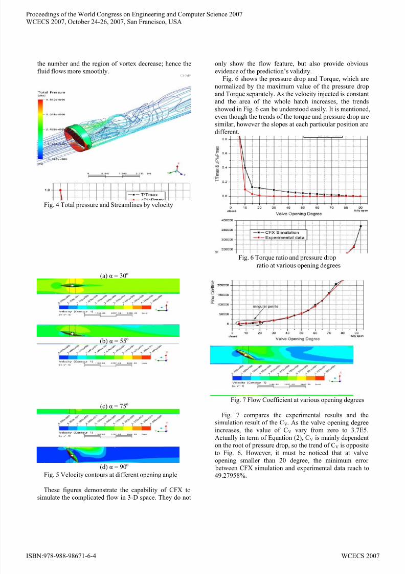
4. Results and DiscussionFig. 4 shows the computed velocity streamlines and

total pressure at the inner surface of valve for the 20o

opening angle. Fig. 5 illustrates the velocity contours on

the middle surface at four different opening degrees. It

can be found that as the valve opening degree increase,

∑∑==

⋅+⋅=n

i x

n

i y z yF xF T

11

)(α (6)

Fig. 3 Method of torque calculation


ISBN:978-988-98671-6-4 WCECS 2007



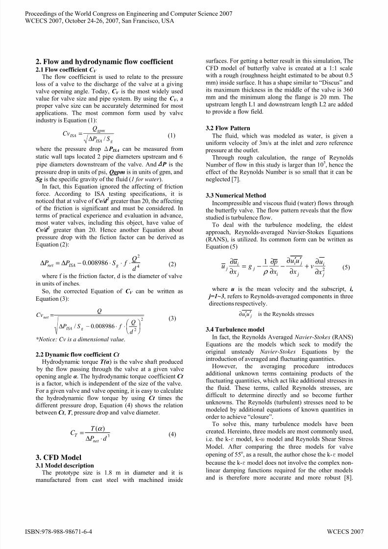
the number and the region of vortex decrease; hence the

fluid flows more smoothly.

Fig. 4 Total pressure and Streamlines by velocity

(a) α = 30o

(b) α = 55o

(c) α = 75o

(d) α = 90o

Fig. 5 Velocity contours at different opening angle

These figures demonstrate the capability of CFX tosimulate the complicated flow in 3-D space. They do not

only show the flow feature, but also provide obvious

evidence of the prediction’s validity.Fig. 6 shows the pressure drop and Torque, which are

normalized by the maximum value of the pressure drop

and Torque separately. As the velocity injected is constant

and the area of the whole hatch increases, the trendsshowed in Fig. 6 can be understood easily. It is mentioned,even though the trends of the torque and pressure drop are

similar, however the slopes at each particular position are

different.

Fig. 6 Torque ratio and pressure drop

ratio at various opening degrees

Fig. 7 Flow Coefficient at various opening degrees

Fig. 7 compares the experimental results and thesimulation result of the CV. As the valve opening degree

increases, the value of CV vary from zero to 3.7E5.

Actually in term of Equation (2), CV is mainly dependenton the root of pressure drop, so the trend of CV is opposite

to Fig. 6. However, it must be noticed that at valve

opening smaller than 20 degree, the minimum error

between CFX simulation and experimental data reach to49.27958%.


ISBN:978-988-98671-6-4 WCECS 2007



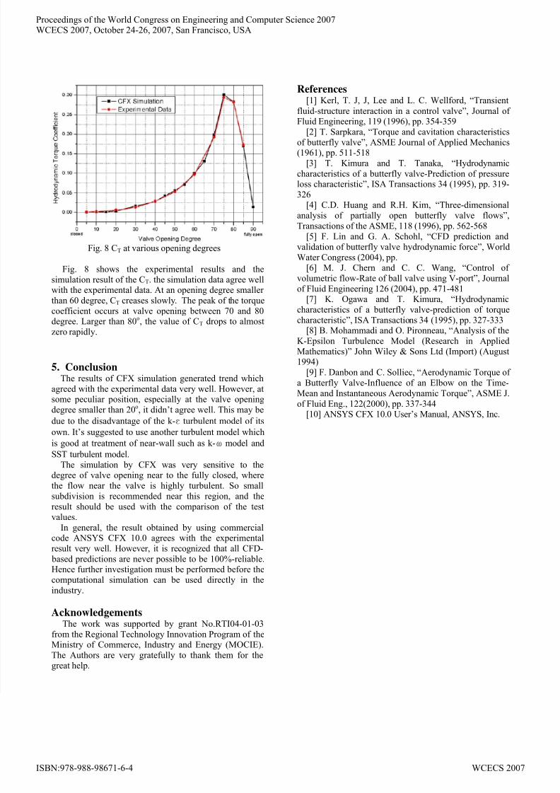
Fig. 8 CT at various opening degrees

Fig. 8 shows the experimental results and the

simulation result of the CT. the simulation data agree wellwith the experimental data. At an opening degree smaller

than 60 degree, CT creases slowly. The peak of the torque

coefficient occurs at valve opening between 70 and 80degree. Larger than 80o, the value of CT drops to almost

zero rapidly.

5. ConclusionThe results of CFX simulation generated trend which

agreed with the experimental data very well. However, atsome peculiar position, especially at the valve opening

degree smaller than 20o, it didn’t agree well. This may be

due to the disadvantage of the k-ε turbulent model of its

own. It’s suggested to use another turbulent model which

is good at treatment of near-wall such as k-ω model and

SST turbulent model.

The simulation by CFX was very sensitive to thedegree of valve opening near to the fully closed, where

the flow near the valve is highly turbulent. So small

subdivision is recommended near this region, and the

result should be used with the comparison of the test

values.

In general, the result obtained by using commercialcode ANSYS CFX 10.0 agrees with the experimental

result very well. However, it is recognized that all CFD-

based predictions are never possible to be 100%-reliable.Hence further investigation must be performed before the

computational simulation can be used directly in the

industry.

AcknowledgementsThe work was supported by grant No.RTI04-01-03

from the Regional Technology Innovation Program of theMinistry of Commerce, Industry and Energy (MOCIE).

The Authors are very gratefully to thank them for thegreat help.

References[1] Kerl, T. J, J, Lee and L. C. Wellford, “Transient

fluid-structure interaction in a control valve”, Journal of Fluid Engineering, 119 (1996), pp. 354-359

[2] T. Sarpkara, “Torque and cavitation characteristics

of butterfly valve”, ASME Journal of Applied Mechanics(1961), pp. 511-518

[3] T. Kimura and T. Tanaka, “Hydrodynamic

characteristics of a butterfly valve-Prediction of pressureloss characteristic”, ISA Transactions 34 (1995), pp. 319-

326[4] C.D. Huang and R.H. Kim, “Three-dimensional

analysis of partially open butterfly valve flows”,

Transactions of the ASME, 118 (1996), pp. 562-568

[5] F. Lin and G. A. Schohl, “CFD prediction and

validation of butterfly valve hydrodynamic force”, World

Water Congress (2004), pp.[6] M. J. Chern and C. C. Wang, “Control of

volumetric flow-Rate of ball valve using V-port”, Journalof Fluid Engineering 126 (2004), pp. 471-481

[7] K. Ogawa and T. Kimura, “Hydrodynamic

characteristics of a butterfly valve-prediction of torque

characteristic”, ISA Transactions 34 (1995), pp. 327-333[8] B. Mohammadi and O. Pironneau, “Analysis of the

K-Epsilon Turbulence Model (Research in Applied

Mathematics)” John Wiley & Sons Ltd (Import) (August1994)

[9] F. Danbon and C. Solliec, “Aerodynamic Torque of

a Butterfly Valve-Influence of an Elbow on the Time-

Mean and Instantaneous Aerodynamic Torque”, ASME J.

of Fluid Eng., 122(2000), pp. 337-344

[10] ANSYS CFX 10.0 User’s Manual, ANSYS, Inc.


ISBN:978-988-98671-6-4 WCECS 2007

Butterfly Valve and Flow

Documents

Transcript of Butterfly Valve and Flow