
Business Statistics 41000: Homework # 2...
24
0.1+0.3+0.4+ P (X =0.1) = 1 P (X =0.1) = 0.20 0.00 0.01 0.02 0.03 0.04 0.05 0.06 0.07 0.08 0.09 0.10 0.11 0.12 0.13 0.14 0.1 0.2 0.3 0.4 0.5 0.6 0.7 0.8 0.9 1.0 X P (X> 0.05) = P (X =0.07) + P (X =0.10) = 0.4+0.2=0.6 E[X ] = 0.02 * 0.1+0.04 * 0.3+0.07 * 0.4+0.1 * 0.2 = 0.002 + 0.012 + 0.028 + 0.02 = 0.062
Transcript of Business Statistics 41000: Homework # 2...

Business Statistics 41000: Homework # 2 Solutions
Drew Creal
February 9, 2014
Question # 1. Discrete Random Variables and Their Distributions
(a) The probabilities have to sum to 1, which means that 0.1 + 0.3 + 0.4 + P (X = 0.1) = 1. We
can therefore deduce that P (X = 0.1) = 0.20.
(b) Here is a plot of the distribution.
0.00 0.01 0.02 0.03 0.04 0.05 0.06 0.07 0.08 0.09 0.10 0.11 0.12 0.13 0.14
0.1
0.2
0.3
0.4
0.5
0.6
0.7
0.8
0.9
1.0
(c) The random variable X can take on two values greater than 0.05. We sum their probabilities:
P (X > 0.05) = P (X = 0.07) + P (X = 0.10) = 0.4 + 0.2 = 0.6.
(d)
E[X] = 0.02 ∗ 0.1 + 0.04 ∗ 0.3 + 0.07 ∗ 0.4 + 0.1 ∗ 0.2
= 0.002 + 0.012 + 0.028 + 0.02
= 0.062
1

(e)
V [X] = 0.1 (0.02− 0.062)2 + 0.3 (0.04− 0.062)2 + 0.4 (0.07− 0.062)2 + 0.2 (0.10− 0.062)2
= 0.1 (−0.042)2 + 0.3 (−0.022)2 + 0.4 (0.008)2 + 0.2 (0.038)2
= 0.1 (0.0018) + 0.3 (0.0005) + 0.4 (0.000064) + 0.2 (0.0014)
= 0.00018 + 0.00015 + 0.0000256 + 0.00028
= 0.000636
(f) The standard deviation is the square root of the variance. We have σX =√σ2X =
√0.00067 =
0.0259

Question # 2. Discrete Random Variables and Their Distributions
(a) The random variable X can only take on two outcomes which are 1 and 0. We are rolling a
�fair� die so that the probability P (X = 1) is the same as the probability that we roll a six
which is P (X = 1) = 16 . The probability that X = 0 is therefore 5
6 . It is important that you
recognize that X ∼ Bernoulli(16
). We can write this in a two-way table:
x p(x)
0 56
1 16
(b) We know that X ∼ Bernoulli(16
). In class, we wrote out the formulas for the mean and variance
of a Bernoulli (p) random variable. These are E[X] = p and V [X] = p(1 − p). Now, we just
plug p = 16 into these formulas to get E[X] = 1
6 and V [X] = 0.139.

Question # 3. Discrete Random Variables and Their Distributions
(a) We just sum the probabilities between 0 and 0.15. P (0 < R < 0.15) = P (R = 0.01) + P (R =
0.05) + P (0.10) = 0.2 + 0.3 + 0.2 = 0.7. Notice that we do not include P (R = 0.15) because
it says less than 0.15 not less than or equal to.
(b) We want to compute P (X < 0) = P (X = −0.05) + P (X = −0.01) = 0.1 + 0.1 = 0.2.
(c) Here, we apply the formula for the expected value that we gave in class.
E[R] = 0.1 ∗ −0.05 + 0.1 ∗ −0.01 + 0.2 ∗ 0.01 + 0.3 ∗ 0.05 + 0.2 ∗ 0.10 + 0.1 ∗ 0.15
= −0.005− 0.001 + 0.002 + 0.015 + 0.02 + 0.015
= 0.046
(d) Here, we �rst compute the variance and then just take the square root.
V [R] = 0.1 (−0.05− 0.046)2 + 0.1 (−0.01− 0.046)2 + 0.2 (0.01− 0.046)2
+0.3 (0.05− 0.046)2 + 0.2 (0.10− 0.046)2 + 0.1 (0.15− 0.046)2
= 0.1 (−0.096)2 + 0.1 (−0.056)2 + 0.2 (−0.036)2 + 0.3 (0.004)2 + 0.2 (0.054)2 + 0.1 (0.104)2
= 0.1 (0.009) + 0.1 (0.003) + 0.2 (0.0013) + 0.3 (0.000002) + 0.2 (0.003) + 0.1 (0.0108)
= 0.0009 + 0.0003 + 0.00026 + 0.0000006 + 0.0006 + 0.00108
= 0.00314
Taking the square root we get σX =√σ2X =
√0.00314 = 0.05604

(e) Here is a plot of the distribution.
−0.050 −0.025 0.000 0.025 0.050 0.075 0.100 0.125 0.150
0.2
0.4
0.6
0.8
1.0
r
p(r)

Question # 4. Marginal and Conditional Distributions of Discrete
Random Variables
(a) Here is the tree diagram.
G = 1 (GOOD)
G = 0
(BAD)
0.5
0.5
0.8
0.2
0.4
0.6
E = 1 P(E = 1 and G = 1) = 0.5 * 0.8 = 0.4
E = 0 P(E = 0 and G = 1) = 0.5 * 0.2 = 0.1
E = 1 P(E = 1 and G = 0) = 0.5 * 0.4 = 0.2
E = 0 P(E = 0 and G = 0) = 0.5 * 0.6 = 0
(b) Given the information from the tree diagram above, we can easily represent it as a two-way
table.
G
0 1 pE(e)
E 0 0.3 0.1 0.4
1 0.2 0.4 0.6
pG(g) 0.5 0.5
(c) Here, we are given P (E = 1|G = 1) but we want to know P (G = 1|E = 1). (NOTE: This
is exactly the same problem as the example from Lecture #3 where we were testing for a
disease.) However, we have already computed the joint distribution of (E,G) and it is simple
to obtain the marginal distributions. Therefore, we can use our formula for the de�nition of

a conditional probability
P (G = 1|E = 1) =P (G = 1, E = 1)
P (E = 1)
=0.4
0.6
= 0.667
One �nal comment to make. In this problem, we have implicitly used Bayes Rule.

Question # 5. Marginal and Conditional Distributions of Discrete
Random Variables
(a) To compute P (X ≤ 0.1, Y ≤ 0.1), we need to add the probabilities.
P (X ≤ 0.1, Y ≤ 0.1) = P (X = 0.05, Y = 0.05) + P (X = 0.1, Y = 0.05)
+P (X = 0.05, Y = 0.1) + P (X = 0.1, Y = 0.1)
= 0.1 + 0.07 + 0.03 + 0.3
= 0.5
(b) To obtain the marginal distribution of X, we simply add each column downwards.
X
0.05 0.10 0.15
Y 0.05 0.10 0.07 0.07
0.10 0.03 0.30 0.03
0.15 0.05 0.05 0.30
pX(x) 0.18 0.42 0.40
Notice that pX(x) is a probability distribution itself because pX(x) = P (X = 0.05) + P (X =
0.10) + P (X = 0.15) = 0.18 + 0.42 + 0.40 = 1. The probabilities sum to one.
(c) To obtain the marginal distribution of Y , we simply add each column across.
X
0.05 0.10 0.15 pY (y)
Y 0.05 0.10 0.07 0.07 0.24
0.10 0.03 0.30 0.03 0.36
0.15 0.05 0.05 0.30 0.40
Notice that pY (y) is also a probability distribution itself because pY (y) = P (Y = 0.05) +
P (Y = 0.10) + P (Y = 0.15) = 0.24 + 0.36 + 0.40 = 1. The probabilities sum to one.
(d) We know the joint probabilities and the marginal probabilites from our work above, therefore
to determine the conditional distribution P (Y = y|X = 0.15) we can use our formulas from

class. Since Y has three outcomes, there are three probabilities that we need to calculate.
P (Y = 0.05|X = 0.15) =P (Y = 0.05, X = 0.15)
P (X = 0.15)
=0.07
0.40= 0.175
P (Y = 0.1|X = 0.15) =P (Y = 0.1, X = 0.15)
P (X = 0.15)
=0.03
0.40= 0.075
P (Y = 0.15|X = 0.15) =P (Y = 0.15, X = 0.15)
P (X = 0.15)
=0.30
0.40= 0.75
Notice that P (Y = y|X = 0.15) is also a probability distribution itself because P (Y =
y|X = 0.15) = P (Y = 0.05|X = 0.15) + P (Y = 0.1|X = 0.15) + P (Y = 0.15|X = 0.15) =
0.175 + 0.075 + 0.75 = 1. The probabilities sum to one.
(e) We know the joint probabilities and the marginal probabilites from our work above, therefore
to determine the conditional distribution P (Y = y|X = 0.05) we can use our formulas from
class. Since Y has three outcomes, there are three probabilities that we need to calculate.
P (Y = 0.05|X = 0.05) =P (Y = 0.05, X = 0.05)
P (X = 0.05)
=0.10
0.18= 0.555
P (Y = 0.1|X = 0.05) =P (Y = 0.1, X = 0.05)
P (X = 0.05)
=0.03
0.18= 0.167
P (Y = 0.15|X = 0.05) =P (Y = 0.15, X = 0.05)
P (X = 0.05)
=0.05
0.18= 0.278
Notice that P (Y = y|X = 0.05) is also a probability distribution itself because P (Y =
y|X = 0.05) = P (Y = 0.05|X = 0.05) + P (Y = 0.1|X = 0.05) + P (Y = 0.15|X = 0.05) =
0.555 + 0.167 + 0.278 = 1. The probabilities sum to one.
(f) By comparing (d) and (e), the distributions are clearly not independent as the conditional dis-

tributions we calculated are not equal to one another nor are they equal to the marginal distri-
bution pY (y). To determine if it is positive or negatively correlated, compare the conditional
distributions P (Y = 0.15|X = 0.15) vs P (Y = 0.15|X = 0.05) and P (Y = 0.05|X = 0.15) vs
P (Y = 0.05|X = 0.05). Notice that conditional on X being small (large), the probabilities
get larger for Y when it is also small (large). Therefore, it is positively correlated.
(g) To calculate the mean and variance of Y , we need to use the marginal probability distribution
from part (c).
E[Y ] = 0.24 ∗ 0.05 + 0.36 ∗ 0.10 + 0.4 ∗ 0.15
= 0.012 + 0.036 + 0.06
= 0.108
V [Y ] = 0.24 (0.05− 0.108)2 + 0.36 (0.10− 0.108)2 + 0.4 (0.15− 0.108)2
= 0.24 (−0.058)2 + 0.36 (−0.008)2 + 0.4 (0.042)2
= 0.24 (0.0034) + 0.36 (0.00006) + 0.4 (0.0018)
= 0.00082 + 0.000022 + 0.00072 = 0.00156
(h) To calculate the conditional mean of the distribution P (Y = y|X = 0.15), we use the proba-
bilities from this distribution.
E[Y |X = 0.15] = 0.175 ∗ 0.05 + 0.075 ∗ 0.10 + 0.75 ∗ 0.15
= 0.0088 + 0.0075 + 0.1125
= 0.128
If we know X = 15% we would guess a higher value for Y because higher values for Y are
more likely when X = 15%.

Question # 6. Sampling WITHOUT replacement and WITH re-
placment
(a) The distribution of Y1 is Bernoulli(.5).
y1 p(y1)
0 12
1 12
(b) P (Y2 = y2|Y1 = 1) is the conditional distribution of the second voter given that we chose a
Democrat on the �rst pick:
y2 P (y2|Y1 = 1)
0 59
1 49
(c) and (d) To write out the joint probability distribution P (Y2 = y2, Y1 = y1) in a table we �rst
need to calculate the entries!
P (Y1 = 1, Y2 = 1) = P (Y2 = 1|Y1 = 1)P (Y1 = 1)
= (4/9) ∗ (1/2) = 0.22
P (Y1 = 1, Y2 = 0) = P (Y2 = 0|Y1 = 1)P (Y1 = 1)
= (5/9) ∗ (1/2) = 0.28
P (Y1 = 0, Y2 = 1) = P (Y2 = 1|Y1 = 0)P (Y1 = 0)
= (5/9) ∗ (1/2) = 0.28
P (Y1 = 0, Y2 = 0) = P (Y2 = 0|Y1 = 0)P (Y1 = 0)
= (4/9) ∗ (1/2) = 0.22
Then, we just put these values in a table. We can calculate the marginal distributions easily
by summing over rows and columns.

Y2
0 1 pY1(y1)
Y1 0 0.22 0.28 0.50
1 0.28 0.22 0.50
pY2(y2) 0.50 0.50
(e) Here, we can use our formulas relating joint distributions to conditional and marginal distri-
butions, i.e. P (Y1 = y1, Y2 = y2, Y3 = y3) = P (Y3 = y3|Y2 = y2, Y1 = y1)P (Y2 = y2|Y1 =
y1)P (Y1 = y1). This formula is applied in the table.
p(y1, y2, y3)
(0,0,0) (1/2)*(4/9)*(3/8) = 0.083
(0,0,1) (1/2)*(4/9)*(5/8) = 0.139
(0,1,0) (1/2)*(5/9)*(4/8) = 0.139
(0,1,1) (1/2)*(5/9)*(4/8) = 0.139
(1,0,0) (1/2)*(5/9)*(4/8) = 0.139
(1,0,1) (1/2)*(5/9)*(4/8) = 0.139
(1,1,0) (1/2)*(4/9)*(5/8) = 0.139
(1,1,1) (1/2)*(4/9)*(3/8) = 0.083
(f) Now, we are sampling WITH replacement! The conditional distribution is:
y2 P (y2|Y1 = 1)
0 510
1 510
You should see that the marginal distribution of Y2 and the conditional distributions of P (Y2 =
y2|Y1 = 0) and P (Y2 = y2|Y1 = 1) are all the same. This is one way we can tell that Y1 and
Y2 are independent.

Question # 7. Independence and Identical Distributions
(a) We can quickly calculate the marginal distributions
Y2
0 1 pY1(y1)
Y1 0 0.067 0.233 0.30
1 0.233 0.467 0.70
pY2(y2) 0.30 0.70
The conditional distributions are
P (Y2 = 1|Y1 = 1) =P (Y2 = 1, Y1 = 0)
P (Y1 = 1)
=0.467
0.70= 0.667
P (Y2 = 0|Y1 = 1) =P (Y2 = 0, Y1 = 1)
P (Y1 = 1)
=0.233
0.70= 0.333
P (Y2 = 1|Y1 = 0) =P (Y2 = 1, Y1 = 0)
P (Y1 = 0)
=0.233
0.30= 0.777
P (Y2 = 0|Y1 = 0) =P (Y2 = 0, Y1 = 1)
P (Y1 = 0)
=0.067
0.30= 0.223
The conditional distributions P (Y2 = y2|Y1 = 1) and P (Y2 = y2|Y1 = 0) are not the same.
They depend on what we observe for Y1. Therefore, they are NOT independent.
(b) The marginal distributions pY1(y1) and pY2(y2) are the same. Therefore, the random variables
are identically distributed. They are not i.i.d. because they are not BOTH independent and
identically distributed.
(c) We are sampling without replacement. If we sampled with replacement, Y1 and Y2 would be
independent (we would put the �rst voter back, so the probability of the second voter being
Democrat would not depend whether the �rst was a Democrat).

(d) We need to calculate the joint probabilities of Y1 and Y2.
P (Y2 = 1, Y1 = 1) = P (Y2 = 1|Y1 = 1)P (Y1 = 1)
= (6999/9999)(7000/10000) = 0.48998
P (Y2 = 0, Y1 = 1) = P (Y2 = 0|Y1 = 1)P (Y1 = 1)
= (2999/9999)(7000/10000) = 0.20996 ≈ 0.21002
P (Y2 = 1, Y1 = 0) = P (Y2 = 1|Y1 = 0)P (Y1 = 0)
= (7000/9999)(3000/10000) = 0.21002
P (Y2 = 0, Y1 = 0) = P (Y2 = 0|Y1 = 0)P (Y1 = 0)
= (2999/9999)(3000/10000) = 0.08998
Notice that the numbers are so large that it really depends on how we round the answers.
Y2
0 1 pY1(y1)
Y1 0 0.08998 0.21002 0.30
1 0.21002 0.48998 0.70
pY2(y2) 0.30 0.70
The conditional probabilities are:
P (Y2 = 1|Y1 = 1) =P (Y2 = 1, Y1 = 1)
P (Y1 = 1)
= (6999/9999) = 0.699969
P (Y2 = 1|Y1 = 0) =P (Y2 = 1, Y1 = 0)
P (Y1 = 1)
= (7000/9999) = 0.700070
The probabilities do depend on what we observe for Y1 but notice that they are very close!
The data is approximately i.i.d..

Question # 8. Covariance, Correlation, Independence and Iden-
tical Distributions
W
5 15 pV (v)
V 5 0.05 0.05 0.10
15 0.45 0.45 0.90
pW (w) 0.50 0.50
X
5 15 pY (y)
Y 5 0.45 0.05 0.50
15 0.05 0.45 0.50
pX(x) 0.50 0.50
(a) First, we need to compute the means of both X and Y using the marginal distributions.
E[X] = 0.5 ∗ 5 + 0.5 ∗ 15 = 10
E[Y ] = 0.5 ∗ 5 + 0.5 ∗ 15 = 10
The covariance between (X,Y ) is
cov(X,Y ) = 0.45 ∗ (5− 10) ∗ (5− 10) + 0.05 ∗ (15− 10) ∗ (5− 10)
+0.05 ∗ (5− 10) ∗ (15− 10) + 0.45 ∗ (15− 10) ∗ (15− 10)
= 0.45 ∗ 25− 0.05 ∗ 25− 0.05 ∗ 25 + 0.45 ∗ 25 = 20
(b) First, we need to compute the means of both W and V using the marginal distributions.
E[W ] = 0.5 ∗ 5 + 0.5 ∗ 15 = 10
E[V ] = 0.1 ∗ 5 + 0.9 ∗ 15 = 14
The covariance between (W,V ) is
cov(W,V ) = 0.05 ∗ (5− 10) ∗ (5− 14) + 0.05 ∗ (15− 10) ∗ (5− 14)
+0.45 ∗ (5− 10) ∗ (15− 14) + 0.45 ∗ (15− 10) ∗ (15− 14)
= 0.05 ∗ 45− 0.05 ∗ 45− 0.45 ∗ 5 + 0.45 ∗ 5 = 0
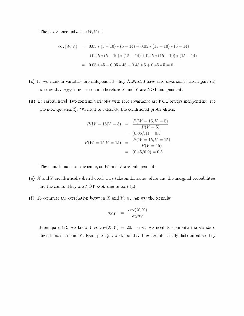
(c) If two random variables are independent, they ALWAYS have zero covariance. From part (a)
we saw that σXY is not zero and therefore X and Y are NOT independent.
(d) Be careful here! Two random variables with zero covariance are NOT always independent (see
the next question!!). We need to calculate the conditional probabilities.
P (W = 15|V = 5) =P (W = 15, V = 5)
P (V = 5)
= (0.05/.1) = 0.5
P (W = 15|V = 15) =P (W = 15, V = 15)
P (V = 15)
= (0.45/0.9) = 0.5
The conditionals are the same, so W and V are independent.
(e) X and Y are identically distributed: they take on the same values and the marginal probabilities
are the same. They are NOT i.i.d. due to part (c).
(f) To compute the correlation between X and Y , we can use the formula:
ρX,Y =cov(X,Y )
σXσY
From part (a), we know that cov(X,Y ) = 20. First, we need to compute the standard
deviations of X and Y . From part (e), we know that they are identically distributed so they

have the same mean and the same variance (standard deviations).
V [X] = 0.5 ∗ (5− 10)2 + 0.5 ∗ (15− 10)2
= 0.5 ∗ 25 + 0.5 ∗ 25
= 25
σx = σy =√25 = 5
This implies that
ρX,Y =cov(X,Y )
σXσY
=20
25= 4/5

Question # 9. Covariance, Correlation, Independence and Iden-
tical Distributions
(a) First, we need to compute the means of both X and Y using the marginal distributions. The
marginal distributions are
X
-1 0 1 pY (y)
Y 0 0 13 0 1
3
1 13 0 1
323
pX(x) 13
13
13
and therefore we get
E[X] =1
3∗ −1 + 1
3∗ 0 + 1
3∗ 1 = 0
E[Y ] =1
3∗ 0 + 2
3∗ 1 =
2
3
The covariance between (X,Y ) is (here in the calculations we only take into consideration
those combinations with non-zero joint probability)
cov(X,Y ) = 0.333 ∗ (0− 0) ∗ (0− 0.667) + 0.333 ∗ (−1− 0) ∗ (1− 0.667)
+0.333 ∗ (1− 0) ∗ (1− 0.667)
= 0

(b) The conditional probabilities can be calculated as:
P (Y = 1|X = −1) =P (Y = 1, X = −1)
P (X = −1)
=1/3
1/3= 1
P (Y = 0|X = −1) =P (Y = 1, X = −1)
P (X = −1)
=0
1/3= 0
P (Y = 1|X = 0) =P (Y = 1, X = −1)
P (X = −1)
=0
1/3= 0
P (Y = 0|X = 0) =P (Y = 1, X = −1)
P (X = −1)
=1/3
1/3= 1
P (Y = 1|X = 1) =P (Y = 1, X = −1)
P (X = −1)
=1/3
1/3= 1
P (Y = 0|X = 1) =P (Y = 1, X = −1)
P (X = −1)
=0
1/3= 0
(c) No. The marginal and conditional probabilities are not the same. These two random variables
have zero covariance but are NOT independent.
(d) Take another look at Y and X. There is a nonlinear relationship between these variables:
Y = X2. Remember, covariance and correlation only measure linear relationships. Here X
and Y are related but not linearly. The point of this question is to drive home the message
that: If X and Y are independent, covariance is ALWAYS zero. If covariance is zero, X and
Y are NOT ALWAYS independent.

Question # 10. Expected Value and Variance of Linear Combina-
tions
First, recognize that Rf is not a random variable. This means that the asset always has a return
of 0.02 no matter what.
(a) Here, we can apply our formulas for expectations of linearly related random variables.
E[P1] = E[.4 ∗Rf + .6 ∗R3]
= .4 ∗Rf + .6 ∗ E[R3]
= .4 ∗ .02 + .6 ∗ .15 = 0.098
(b) Here, we can apply our formulas for the variance of linearly related random variables.
V [P1] = V [.4 ∗Rf + .6 ∗R3]
= (.6)2 ∗ V [R3]
= (0.36) ∗ (0.0225) = 0.0081
It is important to note that Rf drops out from the calculation because it is not a random
variable.
(c) RP1,R3 = 1. The random variables P1 and R3 are linearly related. Therefore, their correlation
is 1.
(d) RP1,R2 = 0. The correlation between R3 and R2 is zero because these random variables are
independent. Taking linear combinations does not change the correlation (Remember problem
# 13 part (g) of Homework # 1) unless you multiply by a negative number which changes
the sign.

(e) Here, we can apply our formulas for expectations of linearly related random variables.
E[P2] = E[0.2 ∗Rf + 0.4 ∗R1 + 0.4R2]
= 0.2 ∗Rf + 0.4 ∗ E[R1] + 0.4 ∗ E[R2]
= 0.2 ∗ .02 + 0.4 ∗ 0.05 + 0.4 ∗ 0.10
= 0.004 + 0.02 + 0.04 = 0.064
(f) Here, we can apply our formulas for the variance of linearly related random variables.
V [P2] = V [0.2 ∗Rf + 0.4 ∗R1 + 0.4R2]
= (0.4)2 ∗ V [R1] + (0.4)2 ∗ V [R2] + 2(0.4)(0.4)corrR1,R2σR1σR2
= 0.16 ∗ (0.05)2 + 0.16 ∗ (0.10)2 + 2(0.4)(0.4)(0.5)(0.05)(0.1)
= 0.0004 + 0.0016 + 0.0008 = 0.0028
(g) P2 is a linear combination of R1 and R2, which are both independent of R3. So corr(P2, R3) =
0. We have not formally shown this but it should make intuitive sense.

Question # 11. Expectation and Variance of Linear Combinations
(a) For each random variable i, we have E[Yi] = E[Wi]− 1 = −1 and V [Yi] = V [Wi] = 10.
E[Z] = E[Y1 + Y2 + Y3]
= E[Y1] + E[Y2] + E[Y3]
= −3
and
V ar[Z] = V ar[Y1 + Y2 + Y3]
= V ar[Y1] + V ar[Y2] + V ar[Y3]
= 30
In the last part, the variance of the sum is equal to the sum of the variances because each Yi
is independent.
(b) We just use our formulas again
E[V ] = E[3W − 1]
= 3E[W ]− 1
= −1
and
V ar[V ] = V ar[3W − 1]
= 9V ar[W ]
= 90
Tripling your bet is more pro�table on average but much riskier.
(c) This is simple if you realize that the mean of a sum is the sum of the means, and since the
W 's are independent, the variance of the sum is the sum of the variances. So since A = 12T ,

E[T ] = E[A] = 0 and V ar[T ] = 20, V ar[A] = 5.
(d)
E[T ] = E
[n∑
i=1
Wi
]=
n∑i=1
E [Wi] = 0
and
V ar[T ] = V ar
[n∑
i=1
Wi
]
=n∑
i=1
V ar [Wi]
=n∑
i=1
10 = 10n
and
E[A] = E
[1
n
n∑i=1
Wi
]=
1
n
n∑i=1
E [Wi] = 0
and
V ar[A] = V ar
[1
n
n∑i=1
Wi
]
=
n∑i=1
V ar
[1
nWi
]
=
n∑i=1
1
n210 =
10
n
(e)
E[X] = E
[1
n
n∑i=1
Xi
]
=1
n
n∑i=1
E [Xi]
=1
n
n∑i=1
µ
= µ

and
V ar[X] = V ar
[1
n
n∑i=1
Xi
]
=n∑
i=1
V ar
[1
nXi
]
=n∑
i=1
1
n2σ2 =
σ2
n


![©2014 Check Point Software Technologies Ltd. 41000 Introduction [Confidential] For designated groups and individuals.](https://static.fdocuments.us/doc/165x107/56649ea25503460f94ba60ac/2014-check-point-software-technologies-ltd-41000-introduction-confidential.jpg)
