Business Process Veri cation with Constraint Temporal...
24
1 Business Process Verification with Constraint Temporal Answer Set Programming * Laura Giordano DISIT, Universit` a del Piemonte Orientale, Italy Alberto Martelli, Matteo Spiotta Dipartimento di Informatica, Universit` a di Torino, Italy Daniele Theseider Dupr´ e DISIT, Universit` a del Piemonte Orientale, Italy submitted 10 April 2013; revised 23 May 2013; accepted 23 June 2013 Abstract The paper provides a framework for the verification of business processes, based on an extension of answer set programming (ASP) with temporal logic and constraints. The framework allows to capture expressive fluent annotations as well as data awareness in a uniform way. It allows for a declarative specification of a business process but also for encoding processes specified in conventional workflow languages. Verification of temporal properties of a business process, including verification of compliance to business rules, is performed by bounded model check- ing techniques in Answer Set Programming, extended with constraint solving for dealing with conditions on numeric data. 1 Introduction The verification of business process compliance to business rules and regulations has gained a lot of interest in recent years, leading to the development of a process annota- tion approach (Governatori and Sadiq 2009; Weber et al. 2010; Hoffmann et al. 2009): information relevant for compliance verification is added, capturing the semantics of atomic tasks execution through preconditions and effects. The treatment of data in pro- cess verification has also attracted growing interest, with the definition of artifact-centric and data-centric process models (Nigam and Caswell 2003; Deutsch et al. 2009). In this paper we combine the two perspectives and propose a framework, based on Answer Set Programming (ASP) (Gelfond 2007), for the specification and verification of business processes, which integrates the treatment of data in business processes with an expressive treatment of annotations, that allows for the specification of conditional effects of atomic tasks as well as for the definition of causal dependencies among annotations. This semantic specification provides background knowledge common to the process and to the compliance rules to be verified. Following (D’Aprile et al. 2010), annotations are specified by an action theory which defines the direct and indirect effects and the * This research has been partially supported by Regione Piemonte, Project ICT4LAW, and by the Compagnia di San Paolo.
Transcript of Business Process Veri cation with Constraint Temporal...

1
Business Process Verification with ConstraintTemporal Answer Set Programming ∗
Laura Giordano
DISIT, Universita del Piemonte Orientale, Italy
Alberto Martelli, Matteo Spiotta
Dipartimento di Informatica, Universita di Torino, Italy
Daniele Theseider Dupre
DISIT, Universita del Piemonte Orientale, Italy
submitted 10 April 2013; revised 23 May 2013; accepted 23 June 2013
Abstract
The paper provides a framework for the verification of business processes, based on an extensionof answer set programming (ASP) with temporal logic and constraints. The framework allowsto capture expressive fluent annotations as well as data awareness in a uniform way. It allowsfor a declarative specification of a business process but also for encoding processes specifiedin conventional workflow languages. Verification of temporal properties of a business process,including verification of compliance to business rules, is performed by bounded model check-ing techniques in Answer Set Programming, extended with constraint solving for dealing withconditions on numeric data.
1 Introduction
The verification of business process compliance to business rules and regulations has
gained a lot of interest in recent years, leading to the development of a process annota-
tion approach (Governatori and Sadiq 2009; Weber et al. 2010; Hoffmann et al. 2009):
information relevant for compliance verification is added, capturing the semantics of
atomic tasks execution through preconditions and effects. The treatment of data in pro-
cess verification has also attracted growing interest, with the definition of artifact-centric
and data-centric process models (Nigam and Caswell 2003; Deutsch et al. 2009).
In this paper we combine the two perspectives and propose a framework, based on
Answer Set Programming (ASP) (Gelfond 2007), for the specification and verification of
business processes, which integrates the treatment of data in business processes with an
expressive treatment of annotations, that allows for the specification of conditional effects
of atomic tasks as well as for the definition of causal dependencies among annotations.
This semantic specification provides background knowledge common to the process and
to the compliance rules to be verified. Following (D’Aprile et al. 2010), annotations
are specified by an action theory which defines the direct and indirect effects and the
∗ This research has been partially supported by Regione Piemonte, Project ICT4LAW, and by theCompagnia di San Paolo.
2 Laura Giordano et al.
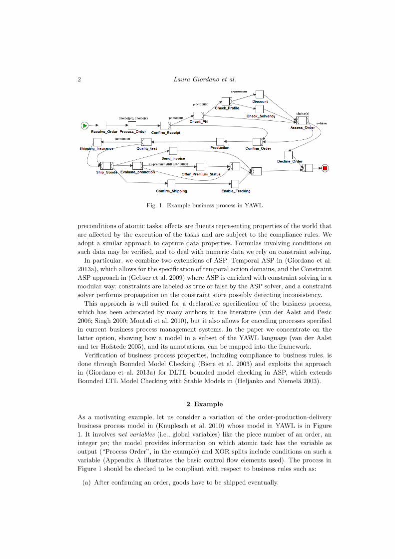
Fig. 1. Example business process in YAWL
preconditions of atomic tasks; effects are fluents representing properties of the world that
are affected by the execution of the tasks and are subject to the compliance rules. We
adopt a similar approach to capture data properties. Formulas involving conditions on
such data may be verified, and to deal with numeric data we rely on constraint solving.
In particular, we combine two extensions of ASP: Temporal ASP in (Giordano et al.
2013a), which allows for the specification of temporal action domains, and the Constraint
ASP approach in (Gebser et al. 2009) where ASP is enriched with constraint solving in a
modular way: constraints are labeled as true or false by the ASP solver, and a constraint
solver performs propagation on the constraint store possibly detecting inconsistency.
This approach is well suited for a declarative specification of the business process,
which has been advocated by many authors in the literature (van der Aalst and Pesic
2006; Singh 2000; Montali et al. 2010), but it also allows for encoding processes specified
in current business process management systems. In the paper we concentrate on the
latter option, showing how a model in a subset of the YAWL language (van der Aalst
and ter Hofstede 2005), and its annotations, can be mapped into the framework.
Verification of business process properties, including compliance to business rules, is
done through Bounded Model Checking (Biere et al. 2003) and exploits the approach
in (Giordano et al. 2013a) for DLTL bounded model checking in ASP, which extends
Bounded LTL Model Checking with Stable Models in (Heljanko and Niemela 2003).
2 Example
As a motivating example, let us consider a variation of the order-production-delivery
business process model in (Knuplesch et al. 2010) whose model in YAWL is in Figure
1. It involves net variables (i.e., global variables) like the piece number of an order, an
integer pn; the model provides information on which atomic task has the variable as
output (“Process Order”, in the example) and XOR splits include conditions on such a
variable (Appendix A illustrates the basic control flow elements used). The process in
Figure 1 should be checked to be compliant with respect to business rules such as:
(a) After confirming an order, goods have to be shipped eventually.

Business Process Verification with Constraint Temporal ASP 3
(b) An order shall either be confirmed or declined.
(c) Orders with a piece number beyond 50000 shall be approved before they are con-
firmed.
(d) For orders of a non-premium customer with a piece number beyond 80000 a solvency
check is necessary before assessing the order.
Such rules hold, except for the last one: for orders of a non-premium customer with a
piece number between 80000 and 100000, flow goes from “Check PN” to “Assess Order”
without executing “Check Solvency”.
Rule verification requires establishing a link between atomic tasks in the business
process and domain properties in rules, especially in case different tasks have effect on the
same property, or tasks have effects on properties that are related to the ones occurring
in the rules. This issue motivates the idea of a semantic annotation of the atomic tasks,
in terms of their effects and preconditions (Governatori and Sadiq 2009). As background
knowledge, in (Weber et al. 2010; Hoffmann et al. 2009) process annotation includes a
domain ontology, namely a theory in clausal form. Our approach to process annotation
builds on work in reasoning about actions and change (Reiter 2001) and, specifically, is
based on the temporal action language in (Giordano et al. 2013a) enriched with constraint
atoms (Gebser et al. 2009) to express conditions on process variables both in the process
model and in rules to be verified, as detailed in the next section.
3 A Constraint Temporal Action Language
In this section we recall the temporal logic DLTL (Henriksen and Thiagarajan 1999) and
the temporal ASP language in (Giordano et al. 2013a), extending them with constraints
in the line of (Gebser et al. 2009).
DLTL extends LTL with temporal operators enriched with program expressions; the
next state modality can be indexed by actions, and the until operator Uπ can be indexed
by a program π which, as in PDL (Harel 1984), can be a regular expression built from
atomic actions using sequence (;), nondeterministic choice (+) and finite iteration (∗).We further extend DLTL allowing, as a base case of formulae, constraints in a lan-
guage C. Such constraints involve a set V of variables, and suitable function and re-
lation symbols, but we will refer to them as constraint atoms since, as in (Gebser
et al. 2009), they will be treated as atoms at the answer set level, and at the tem-
poral logic level. Similarly to (Gebser et al. 2009), a function γ : C → C maps con-
straint atoms to constraints in the sense of (Dechter 2003): each x ∈ V has a domain
dom(x) (which in this paper we assume to be finite), and a constraint c ∈ C is a pair
(S,R) where R is a k-ary relation on a vector S of variables in V: for S = (x1, . . . , xk),
R ⊆ dom(x1)× . . . × dom(xk). For a constraint c = (S,R), let S(c) = S and R(c) = R.
Given an assignment A : V →⋃x∈V dom(x), where A(x) ∈ dom(x), for a constraint
(S,R), with S = (x1, . . . , xk), let A(S) = (A(x1), . . . , A(xk)). The mapping γ provides a
predefined interpretation of the constraint language, i.e., it defines whether an assignment
A satisfies a g ∈ C, which we write A |=γ g and holds iff A(S(γ(g))) ∈ R(γ(g)). E.g., for
the constraint language with variables {x, y, z, . . .}, all with the integer domain, and the
usual arithmetic operators and relations, for which γ provides the usual interpretation,
for the assignment A((x, y, z)) = (10, 20, 15) we have that A |=γ x+ y > z.
4 Laura Giordano et al.
Let Σ = {a1, . . . , an} be a finite non-empty alphabet of actions. Let Σ∗ and Σω be the
set of finite and infinite words on Σ. Let Σ∞ =Σ∗∪Σω. We denote by σ, σ′ the words over
Σω and by τ, τ ′ the words over Σ∗. Moreover, we denote by ≤ the usual prefix ordering
over Σ∗, namely, τ ≤ τ ′ iff ∃τ ′′ such that ττ ′′ = τ ′, and τ < τ ′ iff τ ≤ τ ′ and τ 6= τ ′. For
u ∈ Σ∞, we denote by prf(u) the set of finite prefixes of u.
Let the set of programs (regular expressions) generated by Σ be Prg(Σ) ::= a | π1 +π2
| π1;π2 | π∗, where a ∈ Σ and π1, π2, π range over Prg(Σ). A set of finite words can be
associated with each program by the mapping [[]] : Prg(Σ)→ 2Σ∗ in the usual way.
Let P = {p1, p2, . . .} be a countable set of atomic propositions, let C be a constraint
language, such that, for g ∈ C, γ(g) ∈ C is a constraint on a subset of variables V, with
domains dom(x) for x ∈ V, where D =⋃x∈V dom(x). The set of formulas of DLTL(Σ, C)
is:
DLTL(Σ, C) ::= > | ⊥ | p | g | ¬α | α ∨ β | αUπβ
where > and ⊥ stand for true and false, p ∈ P, g ∈ C, π ∈ Prg(Σ) and α, β range
over DLTL(Σ, C). From the until operator, the derived modalities 〈π〉, [π], © (next), U ,
3 and 2 can be defined as follows: 〈π〉α ≡ >Uπα, [π]α ≡ ¬〈π〉¬α, ©α ≡∨a∈Σ〈a〉α,
αUβ ≡ αUΣ∗β, 3α ≡ >Uα, 2α ≡ ¬3¬α, where, in UΣ∗ , Σ is taken to be a shorthand
for the program a1 + . . .+ an.
A model of DLTL(Σ, C) is a triple M = (σ, V, v) where σ ∈ Σω, V : prf (σ) → 2P
is a valuation function for propositions, and v : prf (σ) → (V → D) provides, for each
τ ∈ prf (σ), an assignment v(τ) for constraint variables. A prefix τ of σ identifies the
state reached after executing τ . Given a model M = (σ, V, v), a prefix τ ∈ prf (σ) and a
formula α, the satisfiability of a formula α at τ in M , written M, τ |= α, is defined as
usual for boolean formulas, and as follows for p ∈ P, g ∈ C and until formulas:
• M, τ |= p iff p ∈ V (τ);
• M, τ |= g iff v(τ) |=γ g;
• M, τ |= αUπβ iff there exists τ ′ ∈ [[π]] such that ττ ′ ∈ prf(σ) and M, ττ ′ |= β.
Moreover, for every τ ′′ such that ε ≤ τ ′′ < τ ′, M, ττ ′′ |= α.
A formula α is satisfiable iff there is a model M = (σ, V, v) and a finite word τ ∈ prf (σ)
such that M, τ |= α.
Observe that, although the extended DLTL language includes (constraint) variables,
we assume that such variables have finite domains; hence, the language is, essentially,
a propositional language, and its decidability follows from the decidability of DLTL
(Henriksen and Thiagarajan 1999).
A domain description is a pair (P,Q), where P is a set of laws describing the effects
and executability preconditions of actions, and Q is a set of DLTL formulas.
Laws in P are defined as follows1. A fluent literal l is a p ∈ P or its negation ¬p. A
constraint literal is a g ∈ C. If l is a fluent literal, or ⊥, representing the inconsistency,
then [a]l,©l (for a ∈ Σ) are temporal fluent literals. If l is a constraint literal, then [a]l,©l(for a ∈ Σ) are temporal constraint literals. We use temporal literal as a shorthand for
temporal (fluent or constraint) literal. Dynamic constraint literals are constraint literals
1 To avoid confusion with constraint variables, we do not define laws with variables, which, as usual inASP, would be a shorthand for the set of their ground instances.

Business Process Verification with Constraint Temporal ASP 5
in the language C extended with variables V◦ = {x◦, for x ∈ V}; variable x◦ represents
“x in the next state”. Given a literal l of any of the types above, not l represents the
default negation of l. A literal, possibly preceded by a default negation, will be called an
extended literal. Laws in P have the form
l0 ← l1, . . . , lm, not lm+1, . . . , not ln (1)
where l0 is a fluent literal or temporal fluent literal, and l1, . . . , ln are fluent literals,
constraint literals, temporal literals or dynamic constraint literals, with the following
restrictions: (i) If l0 is a fluent literal, then the body cannot contain temporal literals or
dynamic constraint literals; (ii) If l0 = [a]l, then the temporal literals in the body must
have the form [a]l′; (iii) If l0 =©l, then the temporal literals in the body must have the
form ©l′.A state is a set of fluent literals and an assignment to constraint variables. A state is
said to be consistent if it is not the case that both f and ¬f belong to the state, or that
⊥ belongs to the state. The execution of an action in a state may possibly change the
values of fluents in the state through its direct and indirect effects, as well as the values
of constraint variables, thus giving rise to a new state. We assume that a law as (1) can
be applied in all states while, when prefixed with Init, it only applies to the initial state.
With the restrictions (i) - (iii) on (1), possible successors of a state S only depend on S.
In (Giordano et al. 2013a) the semantics of a domain description is defined by extending
the notion of answer set (Gelfond 2007) to temporal answer sets, so to capture the linear
structure of temporal models. In particular, the notion of temporal literals is extended
to those of the form [a1; . . . ; ak]l for an action sequence a1; . . . ; ak and a fluent literal l;
a partial temporal interpretation over σ, where σ ∈ Σω, is defined as a pair (σ, S) where
S is a set of temporal literals [a1; . . . ; ak]l, such that a1 . . . ak is a prefix of σ, and S is
required not to contain [a1; . . . ; ak]l where l is the complementary literal of l. Membership
of [a1; . . . ; ak]l in S means that l is true in the state after executing a1 . . . ak.
Temporal answer sets of the first component P of a domain description are defined
in (Giordano et al. 2013a) as partial temporal interpretations, extending the notion of
answer set to compute a different reduct for each prefix a1 . . . ak of a σ. Such a reduct is
a set of rules of the form [a1; . . . ; ak](H ← Body).
In order to extend temporal answer sets to take constraint literals into account, we
follow (Gebser et al. 2009), where a constraint answer set is defined with respect to an
assignment to constraint variables. We then define a constraint temporal answer set with
respect to a v : prf (σ)→ (V [P ]→ D) which provides, for each prefix of σ, an assignment
for variables V [P ] ⊆ V occurring in constraint atoms in P .
Satisfiability of literals is defined extending (Giordano et al. 2013a). Note that while for
temporal (fluent and constraint) literals we take into account the next state, for dynamic
constraint literals the assignments at both the current state and the next one have to be
considered. To simplify the definition, we extend v to v which, for each prefix a1 . . . akof σ, provides an assignment also to variables x◦ ∈ V◦ as follows: v(a1 . . . ak)(x◦) =
v(a1 . . . akak+1)(x) , where a1 . . . akak+1 is a prefix of σ. Then, satisfiability of literals in
(σ, S) at k (where σ = a1 . . . ak, . . .), wrt to a v, is defined as follows, where l is a fluent
literal, g is a constraint or dynamic constraint literal, h is a fluent or constraint literal,
not m is an extended literal:
6 Laura Giordano et al.
(σ, S), v, k 6|= ⊥(σ, S), v, k |= l iff [a1; . . . ; ak]l ∈ S,
(σ, S), v, k |= g iff v(a1 . . . ak) |=γ g
(σ, S), v, k |= [a]h iff (σ, S), v, k + 1 |= h, or a 6= ak+1
(σ, S), v, k |=©h iff (σ, S), v, k + 1 |= h
(σ, S), v, k |= not m iff (σ, S), v, k 6|= m
The following definitions are similar to the definition of constraint reduct in (Gebser
et al. 2009), simplifying or eliminating rules based on the interpretation of constraint
literals; we start by defining the reduct of a single rule for a sequence a1, . . . , ak.
Definition 1The constraint reduct of a rule 2(H ← Body) in P , wrt to (σ, S), to v : prf (σ) →(V [P ]→ D) and to the prefix a1, . . . , ak of σ, is:
• none, if for some (temporal, extended, dynamic) constraint literal l in Body,
(σ, S), v, a1 . . . ak 6|= l• [a1, . . . , ak](H ← Body′) otherwise, where Body′ is Body with (temporal, extended,
dynamic) constraint literals removed.
Definition 2The constraint reduct, P
(σ,S),va1,...,ak , of P relative to (σ, S), to the prefix a1, . . . , ak of σ and
to v : prf (σ)→ (V [P ]→ D), is the set of all the rules
[a1; . . . ; ak](H ← t1, . . . , tm)
such that [a1; . . . ; ak](H ← t1, . . . , tm, not tm+1, . . . , not tn) is the constraint reduct
of a rule in P wrt (σ, S), v and a1, . . . , ak; moreover, (σ, S), a1, . . . , ak 6|= ti, for all
i = m+ 1, . . . , n. The constraint reduct P (σ,S),v of P relative to (σ, S) and v is the union
of all reducts P(σ,S),va1,...,ak for all prefixes a1, . . . , ak of σ.
Definition 3A partial temporal interpretation (σ, S) is a constraint temporal answer set of P wrt v if
(σ, S) is a temporal answer set (Giordano et al. 2013a) of the constraint reduct P (σ,S),v,
i.e., S is minimal among the R such that (σ,R) satisfies the rules in P (σ,S),v.
Well-defined domain descriptions are defined in (Giordano et al. 2013a) as the ones for
which P has total temporal answer sets, and it is observed that total temporal answer
sets correspond to temporal models (as in the semantics of DLTL). The same holds for
the case with constraints, given a v which provides, for the temporal answer set and the
temporal model, the same interpretation for constraint atoms. I.e., given a constraint
temporal answer set (σ, S) of P wrt v, the corresponding temporal model is (σ, VS , v)
where p ∈ VS(a1, . . . , ah) if and only if [a1; . . . ; ah]p ∈ S, for all propositions p ∈ P. This
leads to the following definition of extension of a domain description.
Definition 4An extension of a well-defined domain domain description (P,Q) wrt v is a (total) con-
straint temporal answer set (σ, S) of P wrt v such that the corresponding temporal model
(σ, VS , v) satisfies the formulae in Q.
Verifying that a DLTL(Σ, C) formula α is valid in a well-defined domain description
(P,Q) means checking that there is no extension of (P,Q) satisfying ¬α, i.e., there are
no σ, S, v such that (σ, S) is an extension of (P,Q∪ {¬α}) wrt v.

Business Process Verification with Constraint Temporal ASP 7
4 Process Modeling and Annotation
In (D’Aprile et al. 2010) we proposed to specify annotations in the action theory in
(Giordano et al. 2013a) to define direct and indirect effects of atomic tasks, as well as
their preconditions. In the following we describe how the extended action language with
constraints introduced in section 3 can be used as an annotation language.
An action law has a temporal literal [a]l as head:
[a]l← l1, . . . , lmnot lm+1, . . . , not ln
In case l is a fluent literal, it specifies that, under the conditions in the body, an action
a (a task in the process) has l as a direct effect. In case l is a constraint literal (e.g.,
0 ≤ x ≤ 1000 to represent that a provides a value to x in its domain, or in a subset of a
common domain for all variables) it specifies an effect on process data2.
Nonmonotonic persistence of fluents can also be specified with action laws such as:
[a]f ← f, not [a]¬f
A precondition law is an action law with [a]⊥ as head and it specifies that action a
cannot be executed under the conditions in the body, which can be conditions on fluents,
or constraints on process variables, e.g.:
[a]⊥ ← x ≥ 10000
means that a cannot be executed if x ≥ 10000, i.e., it has x < 10000 as precondition.
Causal laws are used, in reasoning about actions and change, to specify relations be-
tween fluents, and therefore side effects of actions (ramifications). In the action language
in (Giordano et al. 2013a), static causal laws involve fluent literals, while dynamic causal
laws involve temporal fluent literals. For example, the static law f ← g makes f true
whenever g is true, while the dynamic law ©f ← ¬g,©g makes f true when g becomes
true; but f may later be made false while g is still true.
Dynamic causal laws are useful, among other things, for a flexible modeling of processes
with respect to rules they should be compliant with: in particular, to allow for activities
that trigger obligations (e.g., confirming an order triggers the obligation to ship goods)
and activities that cancel them (e.g., if the customer is allowed to cancel the order after
confirmation, this cancels the obligation). Then, rather than verifying that obligations,
once triggered, are eventually fulfilled (in the example, goods are shipped), one should
verify that they are eventually either fulfilled or canceled. In (Giordano et al. 2013b)
we present a general treatment, in our framework, of the types of obligations that in
(Governatori 2010) are pointed out to be relevant for business process verification.
4.1 Declarative vs workflow specification of business processes
In this section we shortly describe how our language can be used for a declarative spec-
ification of business processes as well as for encoding a workflow representation of such
processes.
2 As in (Gebser et al. 2009), a rule c ← Body with a constraint in the head is intended as the (lessreadable) ⊥ ← not c,Body.

8 Laura Giordano et al.
The declarative specification of business processes has been advocated by many authors
(van der Aalst and Pesic 2006; Singh 2000; Montali et al. 2010) as opposed to the more
rigid transition based approach, which can be more constraining than necessary as regards
the order of actions. A declarative specification of a business process can be given by
exploiting the action theory above to define the effects of atomic tasks as well as their
executability preconditions and, possibly, temporal logic constraints.
For instance, the fact than an order can be processed only after it has been re-
ceived can be modeled by a precondition law: [process order]⊥ ← not order received
To guarantee that it will be eventually executed, we can add in C the DLTL formula:
2[receive order]3〈process order〉>.
Observe that, as DLTL is an extension of LTL, it is possible to provide an encoding in
our language of all constraints in the ConDec language (Pesic and van der Aalst 2006).
The additional expressivity, which comes from the presence of program expressions in
DLTL, allows for a very compact encoding of certain declarative properties of the domain
dealing with finite iterations. For instance, the property “action b must be executed
immediately after any even occurrence of action a in a run” can be expressed by the
temporal constraint: 2[(a; Σ∗; a)∗]〈b〉>), where Σ∗ represents any finite action sequence3.
On the other hand, workflow representation is widely used in process management
systems and it represents a natural choice for modeling processes.
A translation from a workflow language to the action theory (or directly to ASP) can
be defined. In particular, the basic constructs of the YAWL language4 can be represented
in the action language as follows, based on the enabling of arcs and tasks (details are
provided in Appendix A). A precondition for the execution of a task a is its being enabled
(represented by a fluent enabled a). Causal laws define that it is enabled when its only
incoming arc is enabled (another fluent), or it is an AND-join and all incoming arcs are
enabled, or it is a XOR-join and one incoming arc is enabled. The execution of a task
disables (in action laws) the incoming arcs and enables the outgoing arcs; in case there is
a nondeterministic XOR-split (named deferred choice in YAWL), the execution of one of
the next tasks also disables arcs corresponding to other choices. For XOR-splits, which in
YAWL have conditions on net variables associated with alternative arcs, such conditions
are included in the action laws for arc enabling. In the example in section 2, the enabling
for outgoing arcs from Confirm Receipt is as follows (an implicit default is intended in
YAWL on the arc to Confirm Order):
[Confirm Receipt]en Confirm Receipt Check PN ← pn > 50000[Confirm Receipt]en Confirm Receipt Confirm Order ← not pn > 50000
Values of a process variable x persist, except in case of tasks a which have x as output
(a piece of information which is in the YAWL model); we represent this as the task having
as effect the fluent change x which is non persistent, and false by default:
x◦ = x←©¬change x[a]change x
3 In (D’Aprile et al. 2010) it has been shown that program expressions can be used to model the controlflow of a business process in a rigid way. However, the solution in (D’Aprile et al. 2010) does not allowto deal with parallelism and non-structured workflows.
4 We refer to YAWL as it is an open system, but our goal is not to reproduce its full semantics, sinceit includes constructs like the OR-join whose semantics is computationally complex.
Business Process Verification with Constraint Temporal ASP 9
¬change x← not change x
5 Translation to ASP
In (Giordano et al. 2013a), a translation of domain descriptions to ASP is defined, as well
as an encoding in ASP of Bounded Model Checking (BMC) (Biere et al. 2003). BMC
looks for paths representing possible executions of a system, and satisfying the required
temporal formulae (including the negation of the formula to be proved valid). It can be
shown that the search can be restricted to infinite paths which can be finitely represented
as paths of length k with a back loop from state k to a previous state in the path. BMC
then searches paths whose finite representation has a length bounded by an integer k,
iteratively increasing k until a run satisfying the required temporal formulae is found (if
one exists). The translation in (Giordano et al. 2013a) is defined so that extensions of
the domain description correspond to answer sets of its ASP translation; in this way, an
ASP solver can be used for finding extensions of (P,Q∪ {¬α}), i.e., counterexamples to
the validity of α in (P,Q).
The translation is based on a representation of states as integers, starting from 0, so
that state i is the state after a prefix a1, . . . , ai of a σ; it uses the predicates:
occurs(Action, State), which means that Action occurs in State, holds(Literal, State),
meaning that Literal is satisfied at State, and sat(Formula, State) meaning that a
DLTL Formula is satisfied at State.
For example, an action law 2([a](¬)f0 ← t1, . . . , tm, not tm+1, . . . , not tn) is translated
to
(¬)holds(f0, S′)← state(S), S′ = S + 1, occurs(a, S), h1 . . . hm, not hm+1 . . . not hn
where hi = (¬)holds(fi, S′) if ti = [a](¬)fi and hi = (¬)holds(fi, S) if ti = (¬)fi.
The translation can be extended to a domain description (P,Q) with constraints in
section 3 as follows, using value(x, S) to represent the value of process variable x in state
S. Following (Gebser et al. 2009), instances of value(x, S) for different instances of S will
be CSP variables in the Constraint ASP program. Each constraint literal g in (P,Q) is
given a unique name name g, and the following rule is added to the definition of sat:
sat(name g, S)← state(S), gS
where gS is g with each variable x replaced with value(x, S). Similarly, for a dynamic
constraint literal d named name d, the rule:
sat(name d, S)← state(S), S′ = S + 1, dS,S′
is added, where dS,S′ is d with variables x ∈ V replaced with value(x, S) and variables
x◦ ∈ V◦ replaced with value(x, S′).
For constraint literals g, [a]g, ©g occurring in laws in P , the translation (exemplified
above for action laws) is similar to the one for non-constraint literals, except that gSand gS′ are used in place of holds(f, S) and holds(f, S′). For dynamic constraint literals,
dS,S′ is used5.
5 Again, as in (Gebser et al. 2009), a rule c← Body with a constraint atom in the head is intended as← not c,Body.
10 Laura Giordano et al.
For example, the translations of the enabling condition for the XOR-split example in
section 4.1, and of the persistence of the value for variable pn are:
holds(en Confirm Receipt Check PN, S′)← state(S), S′ = S + 1,
occurs(Confirm Receipt, S), value(pn, S) $ > 50000
value(pn, S′) $ = value(pn, S)← state(S), S′ = S + 1, not holds(change pn, S′)
where, as in (Gebser et al. 2009), we emphasize with “$” relations in constraint atoms6.
The BMC encoding considers two states different if they differ on fluents (as in (Gior-
dano et al. 2013a)), or on constraint literals in the domain description. In this sense, a
state corresponds to a set of states in the sense of section 3, which assign single values
to variables.
The correspondence results in (Giordano et al. 2013a) still hold. In particular:
Proposition 1
There is a one to one correspondence between the extensions (σ, S) of a domain de-
scription, such that σ can be finitely represented as a finite path with a back loop, and
constraint answer sets (Gebser et al. 2009) of its translation.
The extension and the corresponding constraint answer set R are associated with the
same temporal model (σ, V, v), in particular, an extension wrt v corresponds to an answer
set R wrt a vR, where vR(value(x, s)) = v(a1, . . . , as)(x), with a1, . . . , as ∈ prf(σ).
6 Business process verification
The approach in (Giordano et al. 2013a) is well suited for reasoning about systems with
infinite computations. However, in a YAWL model only executions that reach the end
are considered sound (van der Aalst et al. 2008) (soundness includes other issues and
its verification is a problem by itself, but we do not address it in this paper). To model
this we include the formula 3end in the domain description, where end is a fluent which
becomes true when the end condition is reached; we also introduce a dummy action,
which does not change the state, and it is only executable (and is the only executable
action) when the end condition is reached: its infinite repetition at the end of a finite
execution transforms it in an infinite one with a loop (given by the dummy action). In
practice, as an optimization of the ASP representation of BMC, we can avoid looking for
arbitrary models with loops and restrict to computations corresponding to finite traces.
The basic iterative procedure of BMC is a partial decision procedure for checking
validity: if no model exists, it would never stop. Completeness can be obtained for general
formulae or for special classes of formulae with the techniques described in (Biere et al.
2003; Clarke et al. 2004; Biere et al. 2006; Giordano et al. 2012), and involves identifying
a completeness threshold, i.e. a value t such that validity of a formula α can be checked
without using a value > t for the bound k (i.e., if a model satisfying ¬α exists, one can
be found using bounds up to t). For example, the approach to completeness in (Giordano
6 Since our implementation is based on clingcon, the system in (Gebser et al. 2009; Ostrowski andSchaub 2012), which deals only with the integer domain, the translation of variables with enumer-ated type (like c in the example, for the customer type) departs from the one described above, be-ing based on parametric fluents var(name, value), so that, e.g., a condition c = premium becomesholds(var(c, V ), S), V = premium.
Business Process Verification with Constraint Temporal ASP 11
et al. 2012) could be extended to the language with constraints in this paper. Computing
thresholds, however, is in general challenging from a computational point of view even for
special types of formulae; therefore, existing approaches would not necessarily provide a
feasible solution in a wide range of practical cases. For loop-free workflows, like the one
in the example in section 2, there is a longest run, whose length can be used as threshold.
We experimented the approach on a machine with Intel Xeon E5520 processors (2.26
Ghz) using clingcon (Gebser et al. 2009; Ostrowski and Schaub 2012), and an encoding
with an optimization for the persistence of variable values.
For the example in section 2, rules (c) and (d) can be encoded, respectively, as:
2(pn > 50000 ∧ 〈Confirm Order〉> → a = true) (2)
2(pn > 80000 ∧ c 6= premium ∧ 〈Assess Order〉> → solvency check done) (3)
where solvency check done is an effect of Check Solvency.
The length of the longest run is 21 and can be computed in 1.35 s using the translated
domain description (searching for a run of length k, not necessarily reaching the end, for
increasing values of k, and stopping when no such run is found). Using such a threshold,
validity of (2) can be proved in 0.12 s, and a counterexample for (3) can be found in 0.10
s. If clingcon is not asked to return an assignment of single values to constraint variables,
it computes a weak constraint answer set (Ostrowski 2012), where an approximation of
the restricted domain for variables is given; in this case, in the computed answer set,
the value of pn after Process Order, i.e., value(pn, s) for s ≥ 3, is given the domain
[80001..100000], because the ASP solver assigns true to value(pn, s) > 80000 and false
to value(pn, s) > 100000, and this is consistent for the constraint solver.
Similar running times were obtained for a variation of the example with run length up
to 30 and more complex constraints, where branching is conditioned on the total cost
tc of the order, given by pn ∗ uc (a unit cost, known to be in a given range), possibly
modified by a discount.
In appendix B we report more experiments on the feasibility and scalability of the
approach with current Constraint ASP technology. For the case where the process struc-
ture is a sequence of blocks similar to the one in the running example, we show problems
where verification runs in seconds for processes with up to 200 activities (a size which
is in line with the one of real-world processes in (Fahland et al. 2011)) and run length
of more than 100 activities. The additional cost of constraint solving is acceptable, even
though this does not hold when constraints involve expressions with several variables.
When there is significant parallelism in the process, all the interleavings are considered,
however, verification is shown to run in a minute or less for problems where the number
of different executions is up to 1028.
7 Conclusions and related work
The paper presents an approach to the verification of the compliance of business pro-
cesses, which allows to capture expressive fluent annotations as well as data awareness in
a uniform way. The business process, its semantic annotation and the norms are encoded
using temporal ASP rules, and temporal logic formulae. Compliance verification can be
performed using BMC techniques in Constraint ASP, based on the approach developed

12 Laura Giordano et al.
in (Giordano et al. 2013a) for DLTL bounded model checking in ASP, which extends
the approach for bounded LTL model checking with Stable Models in (Heljanko and
Niemela 2003). This paper enhances the approach to process compliance verification in
(D’Aprile et al. 2010) by taking into consideration the data perspective, and especially
arithmetic constraints, and alternative ways of modeling business processes. The paper
concentrates on business process verification, but the proposed approach can also be
used for the verification of clinical guidelines in the line of (Bottrighi et al. 2010), where,
however, conditions on (numerical) data are not explicit modeled.
In (Knuplesch et al. 2010) a constraint solver is used to compute in advance consistent
sets of conditions on numeric data (occurring in the model and in the formula to be
verified), then performing model checking using such sets as abstractions of actual values.
In our approach, the Constraint ASP solver performs both tasks at once.
The idea of introducing annotations on business processes for compliance verification
has been proposed in (Ghose and Koliadis 2007; Governatori and Sadiq 2009; Weber
et al. 2010). In particular, in (Governatori and Sadiq 2009) annotations and normative
specifications are provided in the same logical language, the Formal Contract Language,
combining Defeasible Logic (Antoniou et al. 2001) and Deontic Logic of Violations (Gov-
ernatori and Rotolo 2006). Compliance is verified by traversing the graph describing the
process and identifying the effects of tasks and the obligations triggered by task execu-
tion. Algorithms for propagating obligations through the process graph are defined.
In (Hoffmann et al. 2009) effects and preconditions of atomic tasks are sets of atomic
formulas, and background knowledge is a theory in clausal form; I-Propagation (Weber
et al. 2010) is exploited for computing annotations. In our approach the domain theory
contains, rather than general clauses, directional causal rules (which avoid unintended
conclusions when reasoning about side effects), and domain annotations are combined
with data properties in a uniform approach.
An annotation approach is also used in (Lu et al. 2006) for the automatic verification
of correctness of workflow models based on Hoare semantics.
In (Deutsch et al. 2009) a service over an artifact schema is defined as a triple: a
precondition, a post-condition and a set of rules in a first-order temporal logic, which
define changes on state relations. The authors identify a class of guarded artifacts for
which verification of properties in a (guarded) first-order extension of LTL is decidable.
In (Damaggio et al. 2011) decidability results are provided for verification with arithmetic
constraints on infinite domains. Our (decidable) language is less expressive, not allowing
for explicit quantification and assuming finite domains for variables.
In (Montali et al. 2010) the Abductive Logic Programming framework SCIFF (Alberti
et al. 2008) is exploited in the declarative specification of business processes as well as in
the verification of their properties. CLP is used for constraints on the timing of events.
In (Alberti et al. 2005) expectations are used for modelling obligations and prohibitions
and norms are formalized by abductive integrity constraints.
In (Roman and Kifer 2008) Concurrent Transaction Logic (CTR) is used to model
and reason about general service choreographies. Service choreographies and contract
requirements are represented in CTR. The paper addresses the problem of deciding if
there is an execution of the service choreography that complies both with the service
policies and the client contract requirements.

Business Process Verification with Constraint Temporal ASP 13
References
Alberti, M., Chesani, F., Gavanelli, M., Lamma, E., Mello, P., and Torroni, P. 2008.Verifiable agent interaction in abductive logic programming: the SCIFF framework. ACMTrans. Comput. Log. 9, 4.
Alberti, M., Gavanelli, M., Lamma, E., Mello, P., Torroni, P., and Sartor, G. 2005.Mapping of Deontic Operators to Abductive Expectations. NORMAS , 126–136.
Antoniou, G., Billington, D., Governatori, G., and Maher, M. J. 2001. Representationresults for defeasible logic. ACM Trans. on Computational Logic 2, 255–287.
Biere, A., Cimatti, A., Clarke, E. M., Strichman, O., and Zhu, Y. 2003. Bounded modelchecking. Advances in Computers 58, 118–149.
Biere, A., Heljanko, K., Juntila, T., Latvala, T., and Schuppan, V. 2006. Linear En-codings of Bounded LTL model checking. Logical Methods in Computer Science 2, 1–64.
Bottrighi, A., Giordano, L., Molino, G., Montani, S., Terenziani, P., and Torchio,M. 2010. Adopting model checking techniques for clinical guidelines verification. ArtificialIntelligence in Medicine 48, 1, 1–19.
Clarke, E., Kroening, D., Ouaknine, J., and Strichman, O. 2004. Completeness andcomplexity of bounded model checking. In VMCAI. 85–96.
Damaggio, E., Deutsch, A., and Vianu, V. 2011. Artifact systems with data dependenciesand arithmetic. In ICDT.
D’Aprile, D., Giordano, L., Gliozzi, V., Martelli, A., Pozzato, G. L., and TheseiderDupre, D. 2010. Verifying business process compliance by reasoning about actions. In CLIMAXI. 99–116.
Dechter, R. 2003. Constraint processing. Elsevier Morgan Kaufmann.
Deutsch, A., Hull, R., Patrizi, F., and Vianu, V. 2009. Automatic verification of data-centric business processes. In ICDT. 252–267.
Fahland, D., Favre, C., Koehler, J., Lohmann, N., Volzer, H., and Wolf, K. 2011.Analysis on demand: Instantaneous soundness checking of industrial business process models.Data Knowl. Eng. 70, 5, 448–466.
Gebser, M., Ostrowski, M., and Schaub, T. 2009. Constraint answer set solving. In ICLP.235–249.
Gelfond, M. 2007. Answer Sets. Handbook of Knowledge Representation, chapter 7, Elsevier .
Ghose, A. and Koliadis, G. 2007. Auditing business process compliance. ICSOC, LNCS4749 , 169–180.
Giordano, L., Martelli, A., and Theseider Dupre, D. 2012. Achieving completeness inbounded model checking of action theories in ASP. In Proc. KR 2012.
Giordano, L., Martelli, A., and Theseider Dupre, D. 2013a. Reasoning about actionswith temporal answer sets. Theory and Practice of Logic Programming 13, 201–225.
Giordano, L., Martelli, A., and Theseider Dupre, D. 2013b. Temporal deontic actionlogic for the verification of compliance to norms in ASP. In Proc. ICAIL 2013.
Governatori, G. 2010. Law, logic and business processes. In Third International Workshopon Requirements Engineering and Law. IEEE.
Governatori, G. and Rotolo, A. 2006. Logic of Violations: A Gentzen System for Reasoningwith Contrary-To-Duty Obligations. Australasian Journal of Logic 4, 193–215.
Governatori, G. and Sadiq, S. 2009. The journey to business process compliance. Handbookof Research on BPM, IGI Global , 426–454.
Harel, D. 1984. Dynamic logic. In Handbook of Philosophical Logic, vol. 2. 497–604.
Heljanko, K. and Niemela, I. 2003. Bounded LTL model checking with stable models. Theoryand Practice of Logic Programming 3, 4-5, 519–550.
14 Laura Giordano et al.
Henriksen, J. and Thiagarajan, P. 1999. Dynamic Linear Time Temporal Logic. Annals ofPure and Applied logic 96, 1-3, 187–207.
Hoffmann, J., Weber, I., and Governatori, G. 2009. On compliance checking for clausalconstraints in annotated process models. Information Systems Frontiers.
Knuplesch, D., Ly, L. T., Rinderle-Ma, S., Pfeifer, H., and Dadam, P. 2010. On en-abling data-aware compliance checking of business process models. In Proc. ER 2010, 29thInternational Conference on Conceptual Modeling. 332–346.
Lu, S., Bernstein, A. J., and Lewis, P. M. 2006. Automatic workflow verification andgeneration. Theor. Comput. Sci. 353, 1-3, 71–92.
Montali, M., Torroni, P., Chesani, F., Mello, P., Alberti, M., and Lamma, E. 2010.Abductive logic programming as an effective technology for the static verification of declarativebusiness processes. Fundam. Inform. 102, 3-4, 325–361.
Nigam, A. and Caswell, N. S. 2003. Business artifacts: An approach to operational specifi-cation. IBM Systems Journal 42, 3, 428445.
Ostrowski, M. 2012. What is this thing called “clingcon”? A language description. Availableat potassco.sourceforge.net.
Ostrowski, M. and Schaub, T. 2012. ASP modulo CSP: The clingcon system. TPLP 12, 4-5,485–503.
Pesic, M. and van der Aalst, W. M. P. 2006. A declarative approach for flexible businessprocesses management. In Business Process Management Workshops, LNCS 4103. Springer,169–180.
Reiter, R. 2001. Knowledge in action. MIT Press.
Roman, D. and Kifer, M. 2008. Semantic web service choreography: Contracting and enact-ment. In International Semantic Web Conference, LNCS 5318. 550–566.
Singh, M. P. 2000. A social semantics for Agent Communication Languages. Issues in AgentCommunication, LNCS(LNAI) 1916 , 31–45.
van der Aalst, W. and ter Hofstede, A. 2005. YAWL: Yet Another Workflow Language.Information Systems 30, 4, 245–275.
van der Aalst, W., van Hee, K., ter Hofstede, A., Sidorova, N., Verbeek, H., Voorho-eve, M., and Wynn, M. 2008. Soundness of Workflow Nets: Classification, Decidability, andAnalysiss. BPM Center Report BPM-08-02, BPMcenter.org .
van der Aalst, W. M. P. and Pesic, M. 2006. Decserflow: Towards a truly declarative serviceflow language. In The Role of Business Processes in Service Oriented Architectures. DagstuhlSeminar Proceedings, vol. 06291.
Weber, I., Hoffmann, J., and Mendling, J. 2010. Beyond soundness: On the verification ofsemantic business process models. Distributed and Parallel Databases (DAPD).
1
Online appendix for the paper
Business Process Verification with ConstraintTemporal Answer Set Programming
published in Theory and Practice of Logic Programming
Laura Giordano
DISIT, Universita del Piemonte Orientale, Italy
Alberto Martelli, Matteo Spiotta
Dipartimento di Informatica, Universita di Torino, Italy
Daniele Theseider Dupre
DISIT, Universita del Piemonte Orientale, Italy
submitted 10 April 2013; revised 23 May 2013; accepted 23 June 2013
Appendix A Representation of control flow
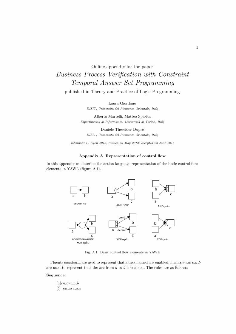
In this appendix we describe the action language representation of the basic control flow
elements in YAWL (figure A 1).
Fig. A 1. Basic control flow elements in YAWL
Fluents enabled a are used to represent that a task named a is enabled, fluents en arc a b
are used to represent that the arc from a to b is enabled. The rules are as follows:
Sequence:
[a]en arc a b
[b]¬en arc a b

2 Laura Giordano et al.
enabled b← en arc a b
¬enabled b← ¬en arc a b
AND-split:
[a]en arc a b [a]en arc a c
[b]¬en arc a b [c]¬en arc a c
enabled b← en arc a b ¬enabled b← ¬en arc a b
enabled c← en arc a c ¬enabled c← ¬en arc a c
AND-join:
[b]en arc b c [a]en arc a c
[c]¬en arc b c [c]¬en arc a c
enabled c← en arc b c, en arc a c
¬enabled c← ¬en arc b c ¬enabled c← ¬en arc a c
Nondeterministic XOR-split:
[a]en arc a b [a]en arc a c
[b]¬en arc a b [b]¬en arc a c
[c]¬en arc a b [c]¬en arc a c
enabled b← en arc a b ¬enabled b← ¬en arc a b
enabled c← en arc a c ¬enabled c← ¬en arc a c
XOR-split:
Analogous to the nondeterministic one, except for the first two rules which become:
[a]en arc a b← Cond [a]en arc a c← not Cond
XOR-join:
[b]en arc b a [c]en arc c a
[a]¬en arc b a [a]¬en arc c a
enabled a← en arc b a enabled a← en arc c a
¬enabled a← ¬en arc b a,¬en arc c a
Online appendix 3
Appendix B Experiments
In this appendix we report some experiments on the feasibility and scalability of the
approach in the paper with current Constraint ASP technology. In particular, we run
in clingcon (Gebser et al. 2009; Ostrowski and Schaub 2012) version 2.0.2 (and in some
cases clingo, version 3.0.3), on a machine with Intel Xeon E5520 processors (2.26Ghz)
and 32 GB RAM, an encoding with an optimization for the persistence of variable values:
rather than propagating values of variables across tasks which do not set their value, a
fluent lastchange(V ar, S, S1) is propagated from S to the next state, representing that
S1 is the last state where the value of V ar was set; therefore, the value of a variable in a
state is actually evaluated in the state where it last changed. This eliminates a number of
equalities on constraint variables (e.g. value(pn, S′) $ = value(pn, S) in section 5) that
should be processed by the constraint solver.
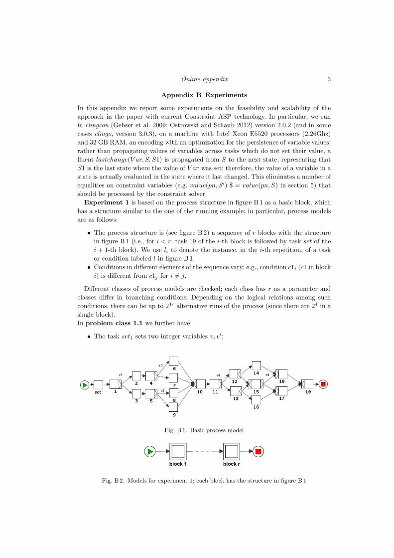
Experiment 1 is based on the process structure in figure B 1 as a basic block, which
has a structure similar to the one of the running example; in particular, process models
are as follows:
• The process structure is (see figure B 2) a sequence of r blocks with the structure
in figure B 1 (i.e., for i < r, task 19 of the i-th block is followed by task set of the
i + 1-th block). We use li to denote the instance, in the i-th repetition, of a task
or condition labeled l in figure B 1.
• Conditions in different elements of the sequence vary; e.g., condition c1i (c1 in block
i) is different from c1j for i 6= j.
Different classes of process models are checked; each class has r as a parameter and
classes differ in branching conditions. Depending on the logical relations among such
conditions, there can be up to 24r alternative runs of the process (since there are 24 in a
single block).
In problem class 1.1 we further have:
• The task set1 sets two integer variables v, v′;
Fig. B 1. Basic process model
Fig. B 2. Models for experiment 1; each block has the structure in figure B 1
4 Laura Giordano et al.
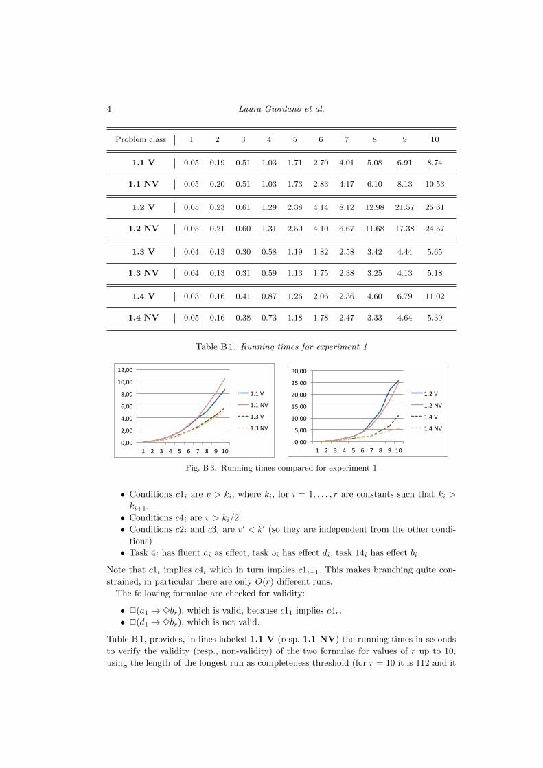
Problem class 1 2 3 4 5 6 7 8 9 10
1.1 V 0.05 0.19 0.51 1.03 1.71 2.70 4.01 5.08 6.91 8.74
1.1 NV 0.05 0.20 0.51 1.03 1.73 2.83 4.17 6.10 8.13 10.53
1.2 V 0.05 0.23 0.61 1.29 2.38 4.14 8.12 12.98 21.57 25.61
1.2 NV 0.05 0.21 0.60 1.31 2.50 4.10 6.67 11.68 17.38 24.57
1.3 V 0.04 0.13 0.30 0.58 1.19 1.82 2.58 3.42 4.44 5.65
1.3 NV 0.04 0.13 0.31 0.59 1.13 1.75 2.38 3.25 4.13 5.18
1.4 V 0.03 0.16 0.41 0.87 1.26 2.06 2.36 4.60 6.79 11.02
1.4 NV 0.05 0.16 0.38 0.73 1.18 1.78 2.47 3.33 4.64 5.39
Table B 1. Running times for experiment 1
0,00
2,00
4,00
6,00
8,00
10,00
12,00
1 2 3 4 5 6 7 8 9 10
1.1 V
1.1 NV
1.3 V
1.3 NV
0,00
5,00
10,00
15,00
20,00
25,00
30,00
1 2 3 4 5 6 7 8 9 10
1.2 V
1.2 NV
1.4 V
1.4 NV
Fig. B 3. Running times compared for experiment 1
• Conditions c1i are v > ki, where ki, for i = 1, . . . , r are constants such that ki >
ki+1.
• Conditions c4i are v > ki/2.
• Conditions c2i and c3i are v′ < k′ (so they are independent from the other condi-
tions)
• Task 4i has fluent ai as effect, task 5i has effect di, task 14i has effect bi.
Note that c1i implies c4i which in turn implies c1i+1. This makes branching quite con-
strained, in particular there are only O(r) different runs.
The following formulae are checked for validity:
• 2(a1 → 3br), which is valid, because c11 implies c4r.
• 2(d1 → 3br), which is not valid.
Table B 1, provides, in lines labeled 1.1 V (resp. 1.1 NV) the running times in seconds
to verify the validity (resp., non-validity) of the two formulae for values of r up to 10,
using the length of the longest run as completeness threshold (for r = 10 it is 112 and it
Online appendix 5
requires 567 seconds to be computed, with more than half time spent to check that there
are no runs of length 113).
In problem class 1.2 we have more complex dependencies among branching conditions;
in particular, we have the following differences wrt 1.1:
• The task seti sets an integer variable vi;• Conditions c1i are vi > ki.• Conditions c2i, c3i are as in 1.1 (and v′ is set by set1).• Conditions c4i are vi > ki/2 for i 6= r
• Condition c4r isr∧
i=1
vi > k′i/2 where k′i < ki (and then vi > ki implies vi > k′i)
In this case, for i 6= r, c1i implies c4i, whiler∧
i=1
c1i implies c4r. The number of different
runs is exponential in r (12r).
The following formulae are checked for validity:
• 2(r∧
i=1
ai → 3br), which is valid, becauser∧
i=1
c1i implies c4r.
• 2(r∧
i=1
di → 3br), which is not valid.
and running times are in lines 1.2 V and 1.2 NV of table B 1.
The approach is sensitive to the way a branching condition is implied by other ones.
For example, if in problem class 1.2 we change c4r to:
r∑i=1
vi >
r∑i=1
ki
which is implied byr∧
i=1
c1i as before, the verification is only feasible up to r = 3.
This behavior is apparently due to the solver integration and the constraint solver
itself (running times increase significantly with the actual size of the numerical domain).
We then further measure the cost of relying, in general, on an integrated solver that
calls a constraint solver for constraint atoms. In two further problem classes, in fact,
we use branching conditions that do not involve constraint atoms, but conditions on
variables with enumerated type; as stated in the paper, their translation does not involve
constraint atoms but just ASP atoms. Therefore, the encoding can be run in clingo.
In particular, problem class 1.3 should be compared with 1.1, in the sense that the
same logical relations hold between branching conditions, but in 1.1 the constraint solver
is responsible for detecting such logical relations.
• set1 sets r + 1 variables v1, . . . , vr+1 with domain {false, true};• Conditions c1i are
r∧j=i∗2−1
vj = true .
• Conditions c2i, c3i are as in 1.1 (and v′ is set by set1).
• Conditions c4i arer∧
j=i∗2vj = true.
As in 1.1, c1i implies c4i which implies c1i+1. The formulae to be verified are as in 1.1
and running times are in lines 1.3 V and 1.3 NV of table B 1; a graphical comparison
for 1.1 and 1.3 is in figure B 3 (left).
Then, in problem class 1.4 (to be compared with 1.2), we have
6 Laura Giordano et al.
• seti sets three variables vai, vbi, vci with domain {false, true};• Conditions c1i are vai = true ∧ vbi = true ∧ vci = true.
• Conditions c2i, c3i are as in 1.1 (and v′ is set by set1).
• Condition c4r isr∧
i=1
vai = true and is implied byr∧
i=1
c1i.
Conditions are related as in 1.2. The formulae to be verified are as in 1.2 and results
are in lines 1.4 V and 1.4 NV of table B 1; a graphical comparison for 1.2 and 1.4 is in
figure B 3 (right).
The results show that the additional cost of relying on a constraint solver is acceptable
for 1.1 and 1.2.
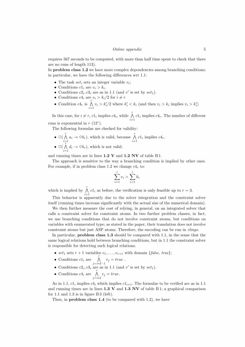
In experiment 2 we tested the case where r blocks, each with the structure in figure
B 1, are in parallel (using AND-split and AND-join), with a single set task that assigns
variables before the split (see figure B 4). Parallel execution means that all interleavings
of every possible execution of each block should in general be considered (no reduction
technique is introduced in our current approach), then the number of possible executions
becomes extremely high even for low values of r.
In problem class 2.1, set assigns variables v1, v2 and for block i we have:
• Conditions c1i are v1 > k1.
• Conditions c2i and c3i are v2 > k2.
• Conditions c4i are v1 > k1/2.
• Task 4i has fluent ai as effect, task 5i has effect di, task 14i has effect bi.
and the following formulae are checked for validity:
• 2r∧
i=1
(ai → 3bi), which is valid.
• 2r∧
i=1
(di → 3bi), which is not valid.
In problem class 2.2, set assigns variables v1,i, v2,i for i = 1, . . . , r and conditions in
block i are as in 2.1, but on v1,i, v2,i.
Fig. B 4. Models for experiment 2; block are as in Figure B 1 with no initial “set” task

Online appendix 7
Problem class 2 3 4 5
2.1 8.4 · 106 1.6 · 1015 1.3 · 1025 1.5 · 1036
2.2 1.0 · 108 2.4 · 1017 2.2 · 1028 3.1 · 1040
Table B 2. Number of different runs for process models in experiment 2
Problem class 2 3 4 5
2.1 V 0.34 2.01 39.48 269.66
2.1 NV 0.23 0.63 72.01 94.24
2.2 V 0.28 2.12 22.79 1239.76
2.2 NV 0.26 0.86 17.46 11594.07
Table B 3. Running times for experiment 2
The number of different executions for r up to 5 is in table B 2.
In spite of such a large search space, verification is feasible (running times are in table
B 3) if the length of the longest run is used as a bound. What is not feasible is computing
such a bound with the approach used in other cases. Of course, if a process model is
hierarchical, e.g. using composite tasks in YAWL, the bound (or an overestimate of it)
can be computed by separately computing the longest activity sequence for component
blocks (composite tasks).
In experiment 3 the process structure is fixed, the one in figure B 5, while branching
conditions of increasing complexity are used, however each variable expression in con-
straint atoms involves a constant and low (3) number of variables. In this case running
times do not explode.
In particular, we have the following conditions which depend on a parameter r and
involve 3r variables set by activity 0:
• Condition c1 isr∧
i=1
v1,i > k1.
• Condition c2 isr∧
i=1
v2,i > k2.
• Condition c6 isr∧
i=1
v3,i > k3.
• Condition c12 isr∧
i=1
v1,i + v2,i + v3,i > k1 + k2 + k3.
• Task 10 has fluent d as effect, task 11 has effect b, task 34 has effect a.
The following formulae are checked for validity:
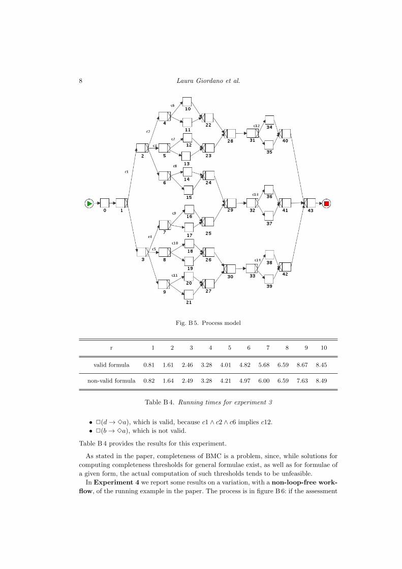
8 Laura Giordano et al.
Fig. B 5. Process model
r 1 2 3 4 5 6 7 8 9 10
valid formula 0.81 1.61 2.46 3.28 4.01 4.82 5.68 6.59 8.67 8.45
non-valid formula 0.82 1.64 2.49 3.28 4.21 4.97 6.00 6.59 7.63 8.49
Table B 4. Running times for experiment 3
• 2(d→ 3a), which is valid, because c1 ∧ c2 ∧ c6 implies c12.
• 2(b→ 3a), which is not valid.
Table B 4 provides the results for this experiment.
As stated in the paper, completeness of BMC is a problem, since, while solutions for
computing completeness thresholds for general formulae exist, as well as for formulae of
a given form, the actual computation of such thresholds tends to be unfeasible.
In Experiment 4 we report some results on a variation, with a non-loop-free work-
flow, of the running example in the paper. The process is in figure B 6: if the assessment
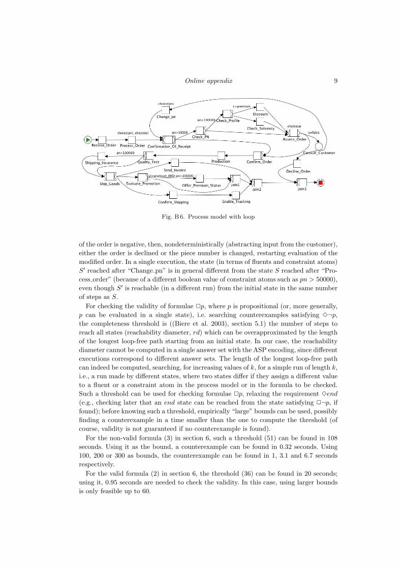
Online appendix 9
Fig. B 6. Process model with loop
of the order is negative, then, nondeterministically (abstracting input from the customer),
either the order is declined or the piece number is changed, restarting evaluation of the
modified order. In a single execution, the state (in terms of fluents and constraint atoms)
S′ reached after “Change pn” is in general different from the state S reached after “Pro-
cess order” (because of a different boolean value of constraint atoms such as pn > 50000),
even though S′ is reachable (in a different run) from the initial state in the same number
of steps as S.
For checking the validity of formulae 2p, where p is propositional (or, more generally,
p can be evaluated in a single state), i.e. searching counterexamples satisfying 3¬p,
the completeness threshold is ((Biere et al. 2003), section 5.1) the number of steps to
reach all states (reachability diameter, rd) which can be overapproximated by the length
of the longest loop-free path starting from an initial state. In our case, the reachability
diameter cannot be computed in a single answer set with the ASP encoding, since different
executions correspond to different answer sets. The length of the longest loop-free path
can indeed be computed, searching, for increasing values of k, for a simple run of length k,
i.e., a run made by different states, where two states differ if they assign a different value
to a fluent or a constraint atom in the process model or in the formula to be checked.
Such a threshold can be used for checking formulae 2p, relaxing the requirement 3end
(e.g., checking later that an end state can be reached from the state satisfying 2¬p, if
found); before knowing such a threshold, empirically “large” bounds can be used, possibly
finding a counterexample in a time smaller than the one to compute the threshold (of
course, validity is not guaranteed if no counterexample is found).
For the non-valid formula (3) in section 6, such a threshold (51) can be found in 108
seconds. Using it as the bound, a counterexample can be found in 0.32 seconds. Using
100, 200 or 300 as bounds, the counterexample can be found in 1, 3.1 and 6.7 seconds
respectively.
For the valid formula (2) in section 6, the threshold (36) can be found in 20 seconds;
using it, 0.95 seconds are needed to check the validity. In this case, using larger bounds
is only feasible up to 60.

10 Laura Giordano et al.
References
Biere, A., Cimatti, A., Clarke, E. M., Strichman, O., and Zhu, Y. 2003. Bounded modelchecking. Advances in Computers 58, 118–149.
Gebser, M., Ostrowski, M., and Schaub, T. 2009. Constraint answer set solving. In ICLP.235–249.
Ostrowski, M. and Schaub, T. 2012. ASP modulo CSP: The clingcon system. TPLP 12, 4-5,485–503.
![Filmstripping and Unrolling: A Comparison of Veri cation ... · model [14], i.e. an equivalent UML/OCL description in which all behavioral model elements and the veri cation task](https://static.fdocuments.us/doc/165x107/5d50380088c993f62d8b72cf/filmstripping-and-unrolling-a-comparison-of-veri-cation-model-14-ie.jpg)