Business Intelligence: Multidimensional Data Analysis · Business Intelligence: Multidimensional...

Business Intelligence:Multidimensional

Data Analysis

Per Westerlund

August 20, 2008Master Thesis in Computing Science

30 ECTS Credits

Abstract

The relational database model is probably the most frequently used database modeltoday. It has its strengths, but it doesn’t perform very well with complex queries andanalysis of very large sets of data. As computers have grown more potent, resulting in thepossibility to store very large data volumes, the need for efficient analysis and processingof such data sets has emerged. The concept of Online Analytical Processing (OLAP)was developed to meet this need. The main OLAP component is the data cube, whichis a multidimensional database model that with various techniques has accomplishedan incredible speed-up of analysing and processing large data sets. A concept that isadvancing in modern computing industry is Business Intelligence (BI), which is fullydependent upon OLAP cubes. The term refers to a set of tools used for multidimensionaldata analysis, with the main purpose to facilitate decision making.

This thesis looks into the concept of BI, focusing on the OLAP technology and datecubes. Two different approaches to cubes are examined and compared; MultidimensionalOnline Analytical Processing (MOLAP) and Relational Online Analytical Processing(ROLAP). As a practical part of the thesis, a BI project was implemented for theconsulting company Sogeti Sverige AB. The aim of the project was to implement aprototype for easy access to, and visualisation of their internal economical data. Therewas no easy way for the consultants to view their reported data, such as how manyhours they have been working every week, so the prototype was intended to propose apossible method. Finally, a performance study was conducted, including a small scaleexperiment comparing the performance of ROLAP, MOLAP and querying against thedata warehouse. The results of the experiment indicates that ROLAP is generally thebetter choice for data cubing.

Table of Contents

List of Figures v

List of Tables vii

Acknowledgements ix

Chapter 1 Introduction 11.1 Business Intelligence . . . . . . . . . . . . . . . . . . . . . . . . . . . . . . 11.2 Background . . . . . . . . . . . . . . . . . . . . . . . . . . . . . . . . . . . 21.3 Problem Statement . . . . . . . . . . . . . . . . . . . . . . . . . . . . . . . 21.4 Goals . . . . . . . . . . . . . . . . . . . . . . . . . . . . . . . . . . . . . . 21.5 Development environment . . . . . . . . . . . . . . . . . . . . . . . . . . . 31.6 Report outline . . . . . . . . . . . . . . . . . . . . . . . . . . . . . . . . . 4

Chapter 2 The Relational Database Model 52.1 Basic definitions . . . . . . . . . . . . . . . . . . . . . . . . . . . . . . . . 52.2 Normalization . . . . . . . . . . . . . . . . . . . . . . . . . . . . . . . . . . 72.3 Indexing . . . . . . . . . . . . . . . . . . . . . . . . . . . . . . . . . . . . . 9

Chapter 3 Online Analytical Processing 133.1 OLAP and Data Warehousing . . . . . . . . . . . . . . . . . . . . . . . . . 133.2 Cube Architectures . . . . . . . . . . . . . . . . . . . . . . . . . . . . . . . 173.3 Relational Data Cubes . . . . . . . . . . . . . . . . . . . . . . . . . . . . . 173.4 Performance . . . . . . . . . . . . . . . . . . . . . . . . . . . . . . . . . . . 20

Chapter 4 Accomplishments 234.1 Overview . . . . . . . . . . . . . . . . . . . . . . . . . . . . . . . . . . . . 234.2 Implementation . . . . . . . . . . . . . . . . . . . . . . . . . . . . . . . . . 244.3 Performance . . . . . . . . . . . . . . . . . . . . . . . . . . . . . . . . . . . 27

Chapter 5 Conclusions 295.1 Why OLAP? . . . . . . . . . . . . . . . . . . . . . . . . . . . . . . . . . . 295.2 Restrictions and Limitations . . . . . . . . . . . . . . . . . . . . . . . . . . 305.3 Future work . . . . . . . . . . . . . . . . . . . . . . . . . . . . . . . . . . . 31

References 34

Appendix A Performance Test Details 35

Appendix B Glossary 43

List of Figures

2.1 Graphical overview of the first three normal forms . . . . . . . . . . . . . 102.2 Example of a B+-tree . . . . . . . . . . . . . . . . . . . . . . . . . . . . . 10

3.1 Example of a star schema . . . . . . . . . . . . . . . . . . . . . . . . . . . 143.2 Example of a snowflake schema . . . . . . . . . . . . . . . . . . . . . . . . 153.3 Graph describing how group by operations can be calculated . . . . . . . 20

4.1 System overview . . . . . . . . . . . . . . . . . . . . . . . . . . . . . . . . 244.2 The data warehouse schema . . . . . . . . . . . . . . . . . . . . . . . . . . 254.3 Excel screenshot . . . . . . . . . . . . . . . . . . . . . . . . . . . . . . . . 264.4 .NET application screenshot . . . . . . . . . . . . . . . . . . . . . . . . . . 27

A.1 Diagrams over query durations . . . . . . . . . . . . . . . . . . . . . . . . 39

List of Tables

2.1 Example of a database relation . . . . . . . . . . . . . . . . . . . . . . . . 62.2 Example of a relation that violates 1NF . . . . . . . . . . . . . . . . . . . 82.3 Example of a relation satisfying 1NF . . . . . . . . . . . . . . . . . . . . . 82.4 Example of a relation satisfying 2NF . . . . . . . . . . . . . . . . . . . . . 9

3.1 Example table of sales for some company . . . . . . . . . . . . . . . . . . 183.2 Example of a pivot table . . . . . . . . . . . . . . . . . . . . . . . . . . . . 183.3 Example result of a cube operation . . . . . . . . . . . . . . . . . . . . . . 193.4 Example result of a rollup operation . . . . . . . . . . . . . . . . . . . . . 193.5 Example of bitmap indexing . . . . . . . . . . . . . . . . . . . . . . . . . . 213.6 Example of bit-sliced indexing . . . . . . . . . . . . . . . . . . . . . . . . . 21

A.1 Performance test data sets . . . . . . . . . . . . . . . . . . . . . . . . . . . 35A.2 Size of the test data . . . . . . . . . . . . . . . . . . . . . . . . . . . . . . 36A.3 Average query durations for the ROLAP . . . . . . . . . . . . . . . . . . . 36A.4 Average query durations for the MOLAP cube . . . . . . . . . . . . . . . 37A.5 Average query durations for the data warehouse, not cached . . . . . . . . 37A.6 Average query durations for the data warehouse, cached . . . . . . . . . . 37A.7 Queries used for the performance test . . . . . . . . . . . . . . . . . . . . 40

Acknowledgements

First of all, I would like to thank my two supervisors: Michael Minock at Umea Univer-sity, Department of Computing Science; and Tomas Agerberg at Sogeti.

I would like to express my gratitude to Sogeti for giving me the opportunity to do mymaster thesis there, and also to all employees who have made my time at the office apleasant stay. I would specifically like to thank, in no particular order, Ulf Smedberg,Ulf Dageryd, Slim Thomsson, Jonas Osterman, Glenn Reian and Erik Lindholm forhelping me out with practical details during my work.

Thanks also to Marie Nordqvist for providing and explaining the Agresso data that Ihave based my practical work on.

Finally I would like to thank Emil Ernerfeldt, Mattias Linde and Malin Pehrsson fortaking the time to proofread my report and for giving me valuable feedback. Thanksalso to David Jonsson for giving me some ideas about the report layout.

1Introduction

This chapter introduces the thesis and Sogeti Sverige AB, the consulting com-pany where it was conducted. A background to the project is given and theproblem specification is stated as well as the project goals and the tools usedduring the process. The chapter ends with an outline of the report.

Business Intelligence (BI) is a concept for analysing collected data with the purposeto help decision making units get a better comprehensive knowledge of a corporation’soperations, and thereby make better business decisions. It is a very popular concept inthe software industry today and consulting companies all over the world have realizedthe need for these services. BI is a type of Decision Support System (DSS), even thoughthis term often has a broader meaning.

One of the consulting companies that are offering BI services is Sogeti Sverige AB,and this master thesis was conducted at their local office in Umea. Sogeti Sverige AB isa part of the Sogeti Group with headquarters in Paris, France, and Capgemini S.A. is theowner of the company group. Sogeti offers IT Solutions in several sectors, for exampleEnergy, Finance & Insurance, Forest & Paper, Transport & Logistics and Telecom.

1.1 Business Intelligence

The BI concept can be roughly decomposed into three parts: collecting data, analysingand reporting.

Collecting data for a BI application is done by building a data warehouse where datafrom multiple heterogeneous data sources is stored. Typical data sources are relationaldatabases, plain text files and spread sheets. Transferring the data from the data sourcesto the data warehouse is often referred to as the Extract, Transform and Load (ETL)process. The data is extracted from the sources, transformed to fit, and finally the datais loaded into the warehouse. The ETL process often brings issues with data consistencybetween data sources; the same data can have a different structure, or the same datacan be found in several data sources without coinciding. In order to load it into the datawarehouse the data has to be consistent, and the process to accomplish this is calleddata cleaning.

A common tool for analysing the data is the data cube, which is a multidimensionaldata structure built upon the data warehouse. The cube is basically used to group databy several dimensions and selecting a subset of interest. This data can be analysed withtools for data mining, which is a concept for finding trends and patterns in the data.

2 Chapter 1. Introduction

The concept of data mining is outside the scope of this thesis and will not be discussedany further.

Finally, reporting is an important issue with BI. Reporting is done by generatingdifferent kinds of reports which often consists of pivot tables and diagrams. Reports canbe uploaded to a report server from which the end user can access them, or the enduser can connect directly to the data source and create ad hoc reports, i.e. based on thestructure of the data cube the user can create a custom report by selecting interestingdata and decide which dimensions to use for organizing it.

When analysing data with BI, a common way of organizing the data is to definekey performance indicators (KPIs), which are metrics used to measure progress towardsorganizational goals. Typical KPIs are revenue and gross operational profit.

1.2 Background

Sogeti is internally using the business and economy system Agresso which holds dataabout each employee, the teams they are organized in, which offices the employees arelocated at, projects the company is currently running, the clients who have orderedthem and so on. There are also economical information such as costs and revenues, andtemporal data that describes when the projects are running and how many hours a weekeach employee has been working on a certain project.

Agresso is used by the administration and decision making units of the company,and the single employee can access some of this data through charts describing themonthly result of the company. A project was initiated to make this data available tothe employees at a more detailed level, but since it had low priority, it remained in it’searly start-up phase until it was adopted as an MT project.

1.3 Problem Statement

Since Agresso is accessible only by the administration and decision making units of theorganisation, the single employee can not even access the data that concerns himself. Theaim of the project was to implement a prototype to make this possible. All employeesshould of course not have access to all data since that would be a threat to the personalintegrity; an ordinary consultant should for example not be able to see how many hoursanother consultant have spent on a certain work related activity. Thus, what data tomake available has to be carefully chosen.

The purpose of the project was to make relevant information available to all employ-ees, by choosing adequate KPIs and letting the employees access those. The preferredway to present this information was by making it available on the company’s intranet.

1.4 Goals

The following is a list of the project goals, each one described in more detail below.

• Identify relevant data

• Build a data warehouse and a data cube

• Present the data to the end user

1.5. Development environment 3

• Automate the process of updating the warehouse and the cube

Identify relevant data

The first goal of the project was to find out what information could be useful, andwhat information should be accessible to the single employee. When analysing this kindof data for trends, KPIs are more useful than raw data, so the information should bepresented as KPIs. There are lots of possible KPIs to use, therefore a few had to bechosen for the prototype.

Build a data warehouse and a data cube

The second goal was to design and implement a data warehouse and a data cube for theAgresso data to be stored. The data warehouse model had to be a robust model basedon the indata structure, designed as a basis for building the data cube. With this cubeit should be possible to browse, sort and group the data based on selected criteria.

Present the data to the end user

The cube data had to be visualized to the end user in some way. Since the data has anatural time dimension, some kind of graph would probably be appropriate. The thirdgoal was to examine different ways of visualizing the data, and to choose a suitable optionfor the prototype. Preferably, the prototype should be available on Sogeti’s intranet.

Automate the process of updating the warehouse and the cube

The process of adding new data and updating the cube should preferably be completelyautomatic. The fourth goal was to examine how this could be accomplished and integratethis functionality in the prototype.

1.5 Development environment

The tools available for the project was Sybase PowerDesigner, Microsoft SQL Server,Microsoft.NET and Dundas Chart. A large part of the practical part of the projectwas to learn these tools, doing this was done by reading books [9, 11, 13] and forums,and by doing several tutorials and reading articles on Microsoft Software DevelopmentNetwork1. The employees at Sogeti has also been a great knowledge base.

PowerDesigner is an easy-to-use graphical tool for database design. With this tool,a conceptual model can be developed using a drag-and-drop interface, after which theactual database can be generated as SQL queries.

Microsoft SQL Server is not only a relational database engine, it also contains threeother important parts used for BI development; Integration Services, Analysis Servicesand Reporting Services.

Integration Services is a set of tools used mainly for managing the ETL process, butit is also usable for scripting and scheduling all kinds of database tasks. With this tool itis possible to automate processes by scheduling tasks that are to be performed regularly.

1See http://www.msdn.com

4 Chapter 1. Introduction

Analysis Services is the tool used for building data cubes. It contains tools forprocessing and deploying the cube as well as designing the cube structure, dimensions,aggregates and other cube related entities.

Reporting Services is used for making reports for the end user, as opposed to thetasks performed by Analysis Services and Integration Services, which are intended forsystem administrators and developers. Reporting Services provides a reporting serverto publish the reports and tools for designing them.

1.6 Report outline

The rest of the report is structured as follows:

Chapter 2. The Relational Database Model explains the basic theory and con-cepts of relational databases, which are very central to data cubes and BusinessIntelligence.

Chapter 3. Online Analytical Processing describes the notion of Data Cubes. Thischapter describes how cubes are designed and used, and it also has a part coveringcube performance.

Chapter 4. Accomplishments describes the accomplishments of the whole project.This includes the implemented prototype, how the work was done and to whatextent the goals were reached, and how the performance tests were made.

Chapter 5. Conclusions sums up the work and discusses what conclusions can bereached.

Appendix A. Performance Test Details contains details of the performance tests,such as the exact queries used and the test result figures.

Appendix B. Glossary contains a list of important terms and abbreviations used inthe report with a short description of each.

2The Relational Database Model

This chapter explains the basic theory behind the relational database model.Basic concepts, including Codd’s first three normal forms, are defined, de-scribed and exemplified.

The relational database model was formulated in a paper by Edgar Frank Codd in1970 [3]. The purpose of the model is to store data in a way that is guaranteed toalways keep the data consistent even in constantly changing databases that are accessedby many users or applications simultaneously. The relational model is a central partof Online Transaction Processing (OLTP), which is what Codd called the whole con-cept of managing databases in a relational manner. Software that is used to handlethe database is referred to as Database Management Systems (DBMS), and the termRelational Database Management Systems (RDBMS) is used to indicate that it is arelational database system. The adjective relational refers to the models fundamentalprinciple that the data is represented by mathematical relations, which are implementedas tables.

2.1 Basic definitions

Definition. A domain D is a set of atomic values. [7]

Atomic in this context means that each value in the domain is indivisible as far asthe relational model is concerned. Domains are often specified with a domain name anda data type for the values contained in the domain.

Definition. A relation schema R, denoted by R(A1, A2, . . . , An), is made up of a rela-tion name R and a list of attributes A1, A2, . . . , An. Each attribute Ai is the name of arole played by some domain D in the relation schema R. D is called the domain of Ai

and is denoted by dom(Ai). [7]

Table 2.1 is an example of a relation represented as a table. The relation is an excerptfrom a database containing clothes sold by some company. The company has severalretailers that sell the products to the customers, and the table contains informationabout what products are available, in which colours they are available, which retailer isselling the product and to what price. According to the above definition, the attributesof the example relation are: Retailer, Product, Colour and Price (e).

Example of related domains are:

• Retailer names: The set of character strings representing all retailer names.

6 Chapter 2. The Relational Database Model

• Clothing products: The set of character strings representing all product names.

• Product colours: The set of character strings representing all colours.

• Product prices: The set of values that represents possible prices of products;i.e. all real numbers.

Retailer Product Colour Price(e)Imaginary Clothing Jeans Blue 40Imaginary Clothing Socks White 10Imaginary Clothing T-shirt Black 15Gloves and T-shirts Ltd. T-shirt Black 12Gloves and T-shirts Ltd. Gloves White 12

Table 2.1: A simple example of a relation represented as a database table.

Definition. A relation (or relation state) r of the relation schema R(A1, A2, . . . , An),also denoted by r(R), is a set of n-tuples r = {t1, t2, . . . , tm}. Each n-tuple t is anordered list of n values t = (v1, v2, . . . , vn), where each value vi, 1 ≤ i ≤ n, is an elementof dom(Ai) or is a special null value. The ith value in tuple t, which corresponds to theattribute Ai, is referred to as t[Ai] (or t[i] if we use the positional notation). [7]

This means that, in the relational model, every table represents a relation r, andeach n-tuple t is represented as a row in the table.

Definition. A functional dependency, denoted by X → Y , between two sets of at-tributes X and Y that are subsets of R specifies a constraint on the possible tuples thatcan form a relation state r of R. The constraint is that, for any two tuples t1 and t2 inr that have t1[X] = t2[X], they must also have t1[Y ] = t2[Y ]. [7]

The meaning of this definition is that if attribute X functionally determines attributeY , then all tuples that have the same value for X, must also have the same value forY . Observe that this definition does not imply Y → X. In Table 2.1, the price ofthe product is determined by the product type and which retailer that sells it, hence{Retailer, Product} → Price. This means that for a certain product sold by a certainretailer, there is only one possible price. Since the opposite is not true, knowing theprice doesn’t necessarily mean that we can determine the product or the retailer; theproduct that costs 12 e could be either the gloves or the t-shirt sold by Gloves andT-shirts Ltd.

Definition. A superkey of a relation schema R = {A1, A2, . . . , An} is a set of attributesS ⊆ R with the property that no two tuples t1 and t2 in any legal relation state r of Rwill have t1[S] = t2[S]. A key K is a superkey with the additional property that removalof any attribute from K will cause K not to be a superkey any more. [7]

Hence, there can be only one row in the database table that has the exact samevalues for all the attributes in the superkey set. Another conclusion of the definitionabove is that every key is a superkey, but there are superkeys that are not keys. Addingan additional attribute to a key set disqualifies it as a key, but it’s still a superkey. Atthe other hand, removing one attribute from a key set disqualifies it as both a superkeyand a key. Since keys and superkeys are sets, they can be made out of single or multipleattributes. In the latter case the key is called a composite key.

2.2. Normalization 7

Definition. If a relation schema has more than one key, each is called a candidate key.One of the candidate keys is arbitrarily designated to be the primary key, and the othersare called secondary keys. [7]

Definition. An attribute of relation schema R is called a prime attribute of R if it is amember of some candidate key of R. An attribute is called nonprime if it is not a primeattribute - that is, if it is not a member of any candidate key. [7]

In a database system, the primary key of each relation is explicitly defined when thetable is created. Primary keys are by convention underlined when describing relationsschematically, and this convention is followed in the examples below. Two underlinedattributes indicates that they both contribute to the key, i.e. it is a composite key.

Definition. A set of attributes FK in relation schema R1 is a foreign key of R1 thatreferences relation R2 if it satisfies both: (a) the attributes in FK have the same do-main(s) as the primary key attributes PK of R2; and (b) a value of FK in a tuple t1 ofthe current state r1(R1) either occurs as a value of PK for some tuple t2 in the currentstate r2(R2) or is null.

Having some attributes in relation R1 forming a foreign key that references relationR2 prohibits data to be inserted into R1 if the foreign key attribute values are not foundin R2. This is a very important referential integrity constraint that avoids references tonon-existing data.

2.2 Normalization

The most important concept of relational databases is normalization. Normalization isdone by adding constraints to how data can be stored in the database, which impliesrestrictions to the way data can be inserted, updated and deleted. The main reasonsfor normalizing database design is to minimize information redundancy and to reducedisk space required to store the database. Redundancy is a problem because it opens upthe possibility to make the database inconsistent. Codd talked about update anomalies,which is classified into three categories; insertion anomalies, deletion anomalies andmodification anomalies [7].

Insertion anomalies occur when a new entry that is not consistent with existingentries is inserted into the database. For example, if a new product sold by ImaginaryClothing is added in Table 2.1, then the name of the company must be spelled theexact same way as all the other entries in the database that contain the company name,otherwise we have two different entries for the same information.

If we assume that Table 2.1 only contains products that currently are available, thenwhat happens when a product, for example gloves, run out of stock? The gloves entrywill be removed from the table, and we have lost the information that the gloves arewhite and that they can be bought from Gloves and T-shirts Ltd. We have even lostthe information that gloves is a product! This is an example of a deletion anomaly.

Finally, suppose that the retailer Gloves and T-shirts Ltd. decides to start sellingjeans too, and therefore they change name to include the new product. All entries inthe database that contain the retailer name must now be updated, or else the databasewill have two different names for the same retailer. This is an example of modificationanomalies.

These issues may seem insignificant when looking at small examples such as theone above, but in a large and complex database that is constantly updated it is very


important that the data is consistent. A normalized database makes sure that everypiece of information is stored in only one place, thus modification of the data only hasto be done once. Storing the same data in one place instead of once per entry will alsosave a lot of storage space.

Normalization is accomplished by designing the database according to the normalforms. Below, Codd’s first three normal forms will be described. Those are the mostcommon normal forms used when designing databases, but there are several other normalforms that are not mentioned here. Each one of the three first normal forms implies thepreceding one, i.e. 3NF implies 2NF, and 2NF implies 1NF.

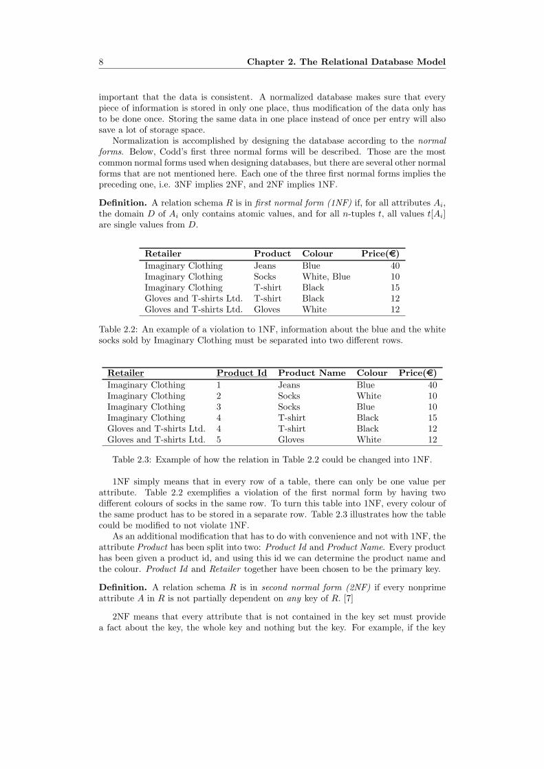
Definition. A relation schema R is in first normal form (1NF) if, for all attributes Ai,the domain D of Ai only contains atomic values, and for all n-tuples t, all values t[Ai]are single values from D.

Retailer Product Colour Price(e)Imaginary Clothing Jeans Blue 40Imaginary Clothing Socks White, Blue 10Imaginary Clothing T-shirt Black 15Gloves and T-shirts Ltd. T-shirt Black 12Gloves and T-shirts Ltd. Gloves White 12

Table 2.2: An example of a violation to 1NF, information about the blue and the whitesocks sold by Imaginary Clothing must be separated into two different rows.

Retailer Product Id Product Name Colour Price(e)Imaginary Clothing 1 Jeans Blue 40Imaginary Clothing 2 Socks White 10Imaginary Clothing 3 Socks Blue 10Imaginary Clothing 4 T-shirt Black 15Gloves and T-shirts Ltd. 4 T-shirt Black 12Gloves and T-shirts Ltd. 5 Gloves White 12

Table 2.3: Example of how the relation in Table 2.2 could be changed into 1NF.

1NF simply means that in every row of a table, there can only be one value perattribute. Table 2.2 exemplifies a violation of the first normal form by having twodifferent colours of socks in the same row. To turn this table into 1NF, every colour ofthe same product has to be stored in a separate row. Table 2.3 illustrates how the tablecould be modified to not violate 1NF.

As an additional modification that has to do with convenience and not with 1NF, theattribute Product has been split into two: Product Id and Product Name. Every producthas been given a product id, and using this id we can determine the product name andthe colour. Product Id and Retailer together have been chosen to be the primary key.

Definition. A relation schema R is in second normal form (2NF) if every nonprimeattribute A in R is not partially dependent on any key of R. [7]

2NF means that every attribute that is not contained in the key set must providea fact about the key, the whole key and nothing but the key. For example, if the key

2.3. Indexing 9

is a composite key, then no attribute is allowed to provide a fact about only one of theprime attributes. Table 2.3 violates 2NF because the product name and the colour isdetermined only by product id, but the primary key for the table is a composition ofproduct id and retailer. Table 2.4 (a) and (b) illustrates a possible decomposition of thetable that doesn’t violate 2NF. Product Id has become the primary key in Table 2.4 (b),and in Table 2.4 (a) it is part of the primary key, but also a foreign key that references(b). Observe also how this restructuring removed the redundancy of the product names.

Retailer Product Id Price (e)Imaginary Clothing 1 40Imaginary Clothing 2 10Imaginary Clothing 3 10Imaginary Clothing 4 15Gloves and T-shirts Ltd. 4 12Gloves and T-shirts Ltd. 5 12

Table 2.4: (a) A decomposition into 2NF of Table 2.3.

Product Id Product Name Colour1 Jeans Blue2 Socks White3 Socks Blue4 T-shirt Black5 Gloves White

Table 2.4: (b) A decomposition into 2NF of Table 2.3.

Definition. A relation schema R is in third normal form (3NF) if, whenever a nontrivialfunctional dependency X → A holds in R, either (a) X is a superkey of R, or (b) A isa prime attribute of R. [7]

The third normal form implies that there can be no transitional dependencies, thatis if A alone is the key attribute, A → B and A → C, then B 9 C must hold.

Figure 2.1 illustrates a schematic view of the functional dependencies allowed by thedifferent normal forms. Key is a single key attribute, prime1 and prime2 is together acomposite key. A and B are attributes that are determined by the key attribute(s), andthe arrows indicates functional dependencies. The figure also illustrates, just as statedabove, that all relations fulfilling the requirements for 3NF also fulfils the requirementsfor 2NF and 1NF.

2.3 Indexing

An important issue of relational databases is how to optimize the database for querying.The most common method is to use indexing, that is having an index structure contain-ing pointers to the actual data in order to optimize search operations. A good indexstructure can increase the performance of a search significantly. The index structurethat is the primary choice for most relational database systems today is the B+-tree [5].


Figure 2.1: Overview of what dependencies are allowed by the first three normal forms.A and B are non-prime attributes, prime1 and prime2 are prime attributes that makesa composite primary key, and key is a single primary key. Functional dependenciesbetween attributes are represented as arrows.

The B+-tree is a tree structure where every node consists of a maximum of d keysand d + 1 pointers. The number d is fixed for a certain tree, but the exact number ofkeys in each node can differ. Each pointer is referring to another tree node, or to theindexed data if the node is a leaf node. The leaf nodes are also linked together withpointers in order to get a fast sequential access. Figure 2.2 illustrates an example, theactual data is marked with a dashed border.

Figure 2.2: An example of a B+-tree, the data that the leaf nodes point to is markedwith a dashed border.

2.3. Indexing 11

To find a specific value in the database, we have to find its key in the tree. Assumewe want to find the value that corresponds to the key X. The search starts in the rootnode, and every key in the current node is compared to X until a key that is equal to orgreater than X is found, or until there are no more keys in the node. When this happens,the associated pointer is followed to the next node, and the procedure is repeated. Thesearch stops when the leaf level is reached and if the key is found there, the data can beretrieved by following the correct pointer.

The B+-tree is always kept balanced, i.e. every leaf node in the tree has the samedepth. This is accomplished by changing the structure of the tree during insertion anddeletion, but the details of these algorithms are not discussed here.

The B+-tree is an advantageous index structure for databases because of its perfor-mance. Maintenance of the structure demands some extra time because of the restruc-turing of the tree when inserting and deleting records, but this loss is small comparedto the gain of searching the tree. The fact that both random and sequential access ispossible is another reason why this type of indexing is so common.

3Online Analytical Processing

This chapter describes the concept of data cubes and data warehousing inthe context of Online Analytical Processing (OLAP). The principles of datacubes are explained as well as how they are designed and what they are usedfor. The relationship between data cubes, data warehouses and relationaldatabases is also examined.

The strength of OLTP databases is that they can perform large amounts of small trans-actions, keeping the database available and the data consistent at all time. The normal-ization discussed in Chapter 2 helps keeping the data consistent, but it also introducesa higher degree of complexity to the database, which causes huge databases to performpoorly when it comes to composite aggregation operations. In the context of businessit is desirable to have historical data covering years of transactions, which results in avast amount of database records to be analyzed. It is not very difficult to realize thatperformance issues will arise when processing analytical queries that requires complexjoining on such databases. Another issue with doing analysis with OLTP is that it re-quire rather complex queries, specially composed for each request, in order to get thedesired result.

3.1 OLAP and Data Warehousing

In order to handle the above issues, the concept of Online Analytical Processing (OLAP)has been proposed and widely discussed through the years and many papers have beenwritten on the subject.

OLTP is often used to handle large amounts of short and repetitive transactions ina constant flow, such as bank transactions or order entries. The database systems aredesigned to keep the data consistent and to maximize transaction throughput. OLAPdatabases are at the other hand used to store historical data over a long period oftime, often collected from several data sources, and the size of a typical OLAP databaseis often orders of magnitude larger than that of an ordinary OLTP database. OLAPdatabases are not updated constantly, but they are loaded on a regular basis such asevery night, every week-end or at the end of the month. This leads to few and largetransactions, and query response time is more important than transaction throughputsince querying is the main usage of an OLAP database [2].

The core of the OLAP technology is the data cube, which is a multidimensionaldatabase model. The model consists of dimensions and numeric metrics which arereferred to as measures. The measures are numerical data such as revenue, cost, sales

14 Chapter 3. Online Analytical Processing

and budget. Those are dependent upon the dimensions, which are used to group thedata similar to the group by operator in relational databases. Typical dimensions aretime, location and product, and they are often organized in hierarchies. A hierarchy is astructure that defines levels of granularity of a dimension and the relationship betweenthose levels. A time dimension can for example have hours as the finest granularity, andhigher up the hierarchy can contain days, months and years. When a cube is queriedfor a certain measure, ranges of one or several dimensions can be selected to filter thedata.

The data cube is based on a data warehouse, which is a central data storage possiblyloaded with data from multiple sources. Data warehouses tend to be very large in size,and the design process is a quite complex and time demanding task. Some companiescould settle with a data mart instead, which is a data warehouse restricted to a depart-mental subset of the whole data set. The data warehouse is usually implemented as arelational database with tables grouped into two categories; dimension tables and facttables.

A dimension table is a table containing data that defines the dimension. A timedimension for example could contain dates, names of the days of the week, week numbers,months names, month numbers and year. A fact table contains the measures, that isaggregatable data that can be counted, summed, multiplied, etc. Fact tables also containreferences (foreign keys) to the dimension tables in the cube so the facts can be groupedby the dimensional data.

A data warehouse is generally structured as a star schema or a snowflake schema.Figure 3.1 illustrates an example of a data warehouse with the star schema structure. Asseen in the figure, a star schema has a fact table in the middle and all dimension tablesare referenced from this table. With a little imagination the setup could be thought ofas star shaped.

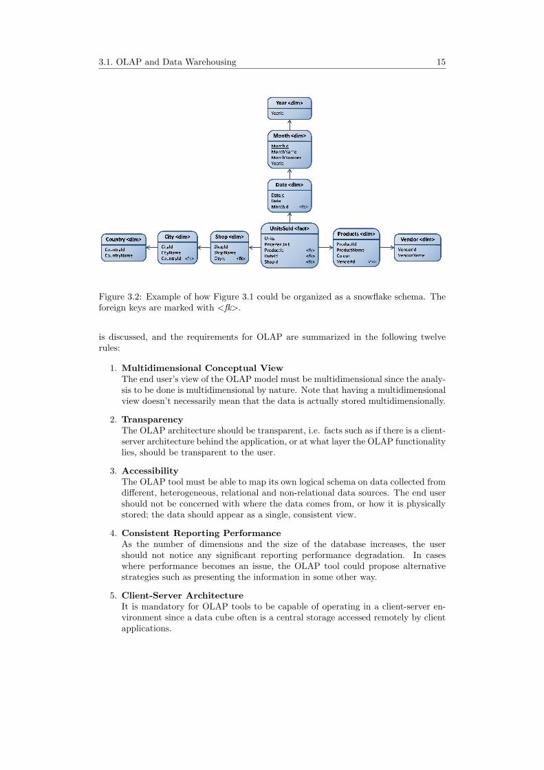
In a star schema, the dimension tables do not have references to other dimensiontables. If they do, the structure is called a snowflake schema instead. A star schemagenerally violates the 3NF by having the dimension tables being several tables joinedtogether, which is often preferred because of the performance loss that 3NF causes whenthe data sets are very large. If it for some reason is desirable to keep the data warehousein 3NF the snowflake schema can be used. Figure 3.2 illustrates an example of howFigure 3.1 could look like if it were to be structured as a snowflake schema.

Figure 3.1: Example of a star schema. The foreign keys are marked with <fk>.

In 1993, Codd et al. published a white paper [4] where the need for OLAP services

3.1. OLAP and Data Warehousing 15

Figure 3.2: Example of how Figure 3.1 could be organized as a snowflake schema. Theforeign keys are marked with <fk>.

is discussed, and the requirements for OLAP are summarized in the following twelverules:

1. Multidimensional Conceptual ViewThe end user’s view of the OLAP model must be multidimensional since the analy-sis to be done is multidimensional by nature. Note that having a multidimensionalview doesn’t necessarily mean that the data is actually stored multidimensionally.

2. TransparencyThe OLAP architecture should be transparent, i.e. facts such as if there is a client-server architecture behind the application, or at what layer the OLAP functionalitylies, should be transparent to the user.

3. AccessibilityThe OLAP tool must be able to map its own logical schema on data collected fromdifferent, heterogeneous, relational and non-relational data sources. The end usershould not be concerned with where the data comes from, or how it is physicallystored; the data should appear as a single, consistent view.

4. Consistent Reporting PerformanceAs the number of dimensions and the size of the database increases, the usershould not notice any significant reporting performance degradation. In caseswhere performance becomes an issue, the OLAP tool could propose alternativestrategies such as presenting the information in some other way.

5. Client-Server ArchitectureIt is mandatory for OLAP tools to be capable of operating in a client-server en-vironment since a data cube often is a central storage accessed remotely by clientapplications.


6. Generic DimensionalityEvery data dimension must be equivalent in structure and operational capabilities.There can be additional features granted to specific dimensions, but the basicstructure must be the same for all dimensions, and thus additional features mustbe possible to grant any dimension.

7. Dynamic Sparse Matrix HandlingA typical data cube is very sparse. Therefore, the OLAP tool should handle sparsematrices in a dynamic way to avoid letting the cube size grow unnecessary. Thereis no need to calculate aggregations for each possible cell in a cube if only a smallfraction of the cells actually contains data.

8. Multi-User SupportOLAP tools must provide concurrent access to the data and the OLAP model, ina way that preserves integrity and security.

9. Unrestricted Cross-dimensional OperationsAn OLAP tool must be able to do calculations and other operations across dimen-sions without requiring the user to explicitly define the actual calculation. Thetool should provide some language for the user to utilize in order to express thedesired operations.

10. Intuitive Data ManipulationDrill-downs, roll-ups and other operations that lie in the nature of dimensionhierarchies1 should be accessible with ease via direct manipulation of the displayeddata, and should not require unnecessary user interface operations such as menunavigation.

11. Flexible ReportingThe reporting should be flexible in the sense that rows, columns and page headersin the resulting report must be able to contain any number of dimensions from thedata model, and that each dimension chosen must be able to display its membersand the relation to them, e.g. by indentation.

12. Unlimited Dimensions and Aggregation LevelsIn the article, Codd et al. states that a serious OLAP tool must be able to handleat least fifteen and preferably twenty dimensions within the same model. Maybethis rule should be extended to allow an unlimited amount of dimensions, just asthe name of the rule implies. In either case, it is also stated that each dimensionmust allow for an unlimited amount of user defined aggregation levels within thedimension hierarchy.

The paper clearly states that OLAP should not be implemented as a new databasetechnology since the relational database model is ‘the most appropriate technology forenterprise databases’. It also states that the relational model never was intended tooffer the services of OLAP tools, but that such services should be provided by separateend-user tools that complements the RDBMS holding the data.

1 Codd et al. use the term consolidation path in their paper, but the term dimension hierarchy ismore common in recent research and literature.

3.2. Cube Architectures 17

3.2 Cube Architectures

Even though the basic cube principles are the same, the cube can be implemented indifferent ways. Different vendors advocate different architectures, and some offers thepossibility to choose an architecture for each cube that is created.

There are two main architectures that traditionally have been discussed in the field ofdatabase research; Multidimensional OLAP (MOLAP) and Relational OLAP (ROLAP).

Multidimensional Online Analytical Processing is based upon the philosophy thatsince the cube is multidimensional in its nature, the data should be stored multidimen-sionally. Thus, the data is copied from the data warehouse to the cube storage andaggregations of different combinations of dimensions are pre-calculated and stored inthe cube in an array based data structure. This means that the query response time isvery short since no calculations has to be done at the time a query is executed. At theother hand, the loading of the cube is an expensive process because of all the calculationsthat have to be done, and therefore the data cube is scheduled to be loaded when it isunlikely to be accessed, on regular intervals such as once every week-end or every night.

A problem that has to be considered when working with MOLAP is data explosion.This is a phenomena that occurs when aggregations of all combinations of dimensionsare to be calculated and stored physically. For each dimension that is added to the cube,the number of aggregations that is to be calculated increases exponentially.

Relational Online Analytical Processing is, just as the name suggests, based on therelational model. The main idea here is that it is better to read data from the datawarehouse directly, than to use another kind of storage for the cube. As is the case withMOLAP, data can be aggregated and pre-calculated in ROLAP too, using materializedviews, i.e. storing the aggregations physically in database tables. A ROLAP architectureis more flexible since it can pre-calculate some of the aggregations, but leave others tobe calculated on request.

Over the years, there has been a great debate in the research field whether OLAPshould be implemented as MOLAP or ROLAP. The debate has however faded, and inthe last decade most researchers seem to argue that ROLAP is superior to MOLAP,among others a white paper from MicroStrategy [10]. The arguments are that ROLAPperform almost as good as MOLAP when there are few dimensions, and when there aretoo many dimensions MOLAP can’t handle it because of the data explosion. Alreadywith about 10-20 dimensions the number of calculations becomes tremendously largein consequence of the exponential growth. Another important aspect is the greaterflexibility of ROLAP; all aggregations don’t need to be calculated beforehand, they canbe calculated on demand as well.

3.3 Relational Data Cubes

One way to implement relational data cubes was proposed by Gray et al. 1997 [8].In this paper the cube operator - which is an n-dimensional generalization of the well-known group by - and the closely related rollup operator is described in detail. The cubeand the rollup operator has been implemented in several relational database engines toprovide data cube operability.

Consider the example figures in Table 3.1. A retailer company has sold jeans andgloves in two colours; black and blue. The total amount of items sold during 2007and 2008 is summed separately for each year and colour in the Sales column. Now, amanager would probably want to look at the figures in the form of sums of the total


Product Year Colour Sales

Jeans 2007 Black 231Jeans 2007 Blue 193Jeans 2008 Black 205Jeans 2008 Blue 236Gloves 2007 Black 198Gloves 2007 Blue 262Gloves 2008 Black 168Gloves 2008 Blue 154

Table 3.1: Example table of sales for some company selling clothing products.

sales during one year, the total amount of jeans sold during 2007, or maybe the amountof blue gloves sold during 2008. One intuitive way to arrange the data for this purposeis to use a pivot table. In this kind of table, data is structured with both row and columnlabels and is also summed along its dimensions in order to get a clear view of the dataset. Table 3.2 is an example of how Table 3.1 could be arranged as a pivot table.

2007 2007 2008 2008Black Blue Total Black Blue Total Grand Total

Jeans 231 193 424 205 236 441 865Gloves 198 262 460 168 154 322 782Grand Total 429 455 884 373 390 763 1647

Table 3.2: Example of a pivot table.

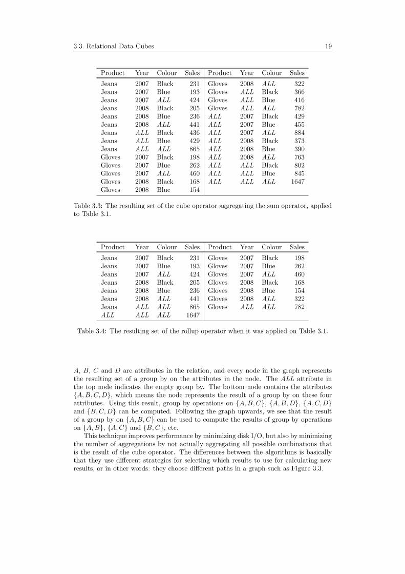
The cube operator expresses the pivot table data set in a relational database context.This operator is basically a set of group by clauses put together with a union operation.It groups the data by the given dimensions (attributes), in this case Product, Year andColour, and aggregations are made for all possible combinations of dimensions. Table 3.3illustrates the resulting data set when the cube operator is used combined with the SUMoperator.

The special ALL value has been introduced to indicate that a certain record containsan aggregation over the attribute that has this value. The NULL value can be usedinstead of the ALL value in order not to manipulate the SQL language.

The cube operator results in a lot of aggregations, but all aggregated combinationsare seldom desired and therefore the rollup operator was also proposed. This operatorworks the same way as the cube operator, but with the difference that new aggregationsare calculated only from already calculated aggregations. Table 3.4 illustrates the resultsfrom a rollup operation.

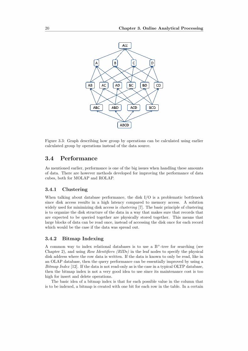
Algorithms have been developed in order to improve the performance of the cubeoperator and a few of those are compared by Agarwal et al. [1]. All of the algorithmscompared utilize the fact that an aggregation using a group by operation (below simplycalled a group by) in general does not have to be computed from the actual relation,but can be computed from the result of another group by. Therefore only one group byreally has to be computed from the relation, namely the one with the finest granularity,and all the others can be computed from this result.

Figure 3.3 illustrates how group by results can be used to compute other aggregations.

3.3. Relational Data Cubes 19

Product Year Colour Sales Product Year Colour Sales

Jeans 2007 Black 231 Gloves 2008 ALL 322Jeans 2007 Blue 193 Gloves ALL Black 366Jeans 2007 ALL 424 Gloves ALL Blue 416Jeans 2008 Black 205 Gloves ALL ALL 782Jeans 2008 Blue 236 ALL 2007 Black 429Jeans 2008 ALL 441 ALL 2007 Blue 455Jeans ALL Black 436 ALL 2007 ALL 884Jeans ALL Blue 429 ALL 2008 Black 373Jeans ALL ALL 865 ALL 2008 Blue 390Gloves 2007 Black 198 ALL 2008 ALL 763Gloves 2007 Blue 262 ALL ALL Black 802Gloves 2007 ALL 460 ALL ALL Blue 845Gloves 2008 Black 168 ALL ALL ALL 1647Gloves 2008 Blue 154

Table 3.3: The resulting set of the cube operator aggregating the sum operator, appliedto Table 3.1.

Product Year Colour Sales Product Year Colour Sales

Jeans 2007 Black 231 Gloves 2007 Black 198Jeans 2007 Blue 193 Gloves 2007 Blue 262Jeans 2007 ALL 424 Gloves 2007 ALL 460Jeans 2008 Black 205 Gloves 2008 Black 168Jeans 2008 Blue 236 Gloves 2008 Blue 154Jeans 2008 ALL 441 Gloves 2008 ALL 322Jeans ALL ALL 865 Gloves ALL ALL 782ALL ALL ALL 1647

Table 3.4: The resulting set of the rollup operator when it was applied on Table 3.1.

A, B, C and D are attributes in the relation, and every node in the graph representsthe resulting set of a group by on the attributes in the node. The ALL attribute inthe top node indicates the empty group by. The bottom node contains the attributes{A,B, C, D}, which means the node represents the result of a group by on these fourattributes. Using this result, group by operations on {A,B, C}, {A,B, D}, {A,C, D}and {B,C,D} can be computed. Following the graph upwards, we see that the resultof a group by on {A,B, C} can be used to compute the results of group by operationson {A,B}, {A,C} and {B,C}, etc.

This technique improves performance by minimizing disk I/O, but also by minimizingthe number of aggregations by not actually aggregating all possible combinations thatis the result of the cube operator. The differences between the algorithms is basicallythat they use different strategies for selecting which results to use for calculating newresults, or in other words: they choose different paths in a graph such as Figure 3.3.


Figure 3.3: Graph describing how group by operations can be calculated using earliercalculated group by operations instead of the data source.

3.4 Performance

As mentioned earlier, performance is one of the big issues when handling these amountsof data. There are however methods developed for improving the performance of datacubes, both for MOLAP and ROLAP.

3.4.1 Clustering

When talking about database performance, the disk I/O is a problematic bottlenecksince disk access results in a high latency compared to memory access. A solutionwidely used for minimizing disk access is clustering [7]. The basic principle of clusteringis to organize the disk structure of the data in a way that makes sure that records thatare expected to be queried together are physically stored together. This means thatlarge blocks of data can be read once, instead of accessing the disk once for each recordwhich would be the case if the data was spread out.

3.4.2 Bitmap Indexing

A common way to index relational databases is to use a B+-tree for searching (seeChapter 2), and using Row Identifiers (RIDs) in the leaf nodes to specify the physicaldisk address where the row data is written. If the data is known to only be read, like inan OLAP database, then the query performance can be essentially improved by using aBitmap Index [12]. If the data is not read-only as is the case in a typical OLTP database,then the bitmap index is not a very good idea to use since its maintenance cost is toohigh for insert and delete operations.

The basic idea of a bitmap index is that for each possible value in the column thatis to be indexed, a bitmap is created with one bit for each row in the table. In a certain

3.4. Performance 21

bitmap, all bits that correspond to the represented value is set to ‘1’ and all other bitsare set to ‘0’.

Product Colour B1 B2 B3

Jeans Blue 1 0 0Socks Black 0 0 1T-shirt Black 0 0 1T-shirt Blue 1 0 0Gloves White 0 1 0

Table 3.5: An example of bitmap indexing.

Table 3.5 illustrates the idea of a bitmap index; it contains a few products and theircolours, where the colour column is the one to be indexed. For every possible colour, abitmap Bi is created that keeps track of all tuples in the relation that has that colour asthe value, e.g. all tuples with the attribute value ‘Blue’ is represented by B1=‘10010’.

Provided that the cardinality of a column isn’t too high, i.e. the number of possiblevalues for that column isn’t too large, there are two improvements introduced by bitmapindices. The first is that the disk size required to store the indices are reduced comparedto using B+-trees. In the above example, three bits are required for each value, comparedto the size of a disk address when using RIDs. The second improvement is performance.The bitwise operators AND, OR and NOT are very fast, and using those it is possibleto execute queries with complex WHERE clauses in a very efficient way. Aggregationoperations like SUM and AVG is also affected by the choice of index.

It doesn’t take long to realize that a bitmap index isn’t of much use if the value tobe indexed is an integer which can have several thousand possible values. Instead, avariant called bit-sliced index can be used in such cases to preserve the benefit of bitmapindices. We assume that the target column is populated by integer values representedby N bits. The bit-slice index assign one bitmap for each of the N bits, instead of onebitmap for each possible value. Table 3.6 illustrates the idea; the amount of sold itemsfor each product is represented by its binary encoding with column B3 representing theleast significant and column B1 representing the most significant bit. Reading thesebinary codes column by column gives the bitmaps in the index, e.g. B1 = ‘1100’.

Product Amount sold B1 B2 B3

Jeans 5 1 0 1Socks 7 1 1 1T-shirt 3 0 1 1Gloves 2 0 1 0

Table 3.6: An example of bit-sliced indexing.

Using this index method, a great query performance increase will will be gained whenit comes to aggregating.

If a relation scheme has a high cardinality, the size of the bitmap index will growlarge rather quickly because every possible value will give rise to another bitmap, with asmany bits as there are tuples in the relation. In these cases there are efficient compressiontechniques that reduce the bitmap sizes.

Two common compression schemes that have these properties are the byte-aligned


bitmap code (BBC) and the word-aligned hybrid code (WAH), examined thoroughly byWu, Otoo and Shoshani [14, 15]. The BBC is based on byte operations and the WAH is avariant of BBC that is based on words which helps word-based CPUs handle this schememore efficiently. Basically, both methods work by finding sequences of consecutive bitsthat have the same value, and replacing these with the bit value and a counter thatkeeps track of how many bits there are in the sequence. Wu et al. have shown thatthese compression techniques result in indices that in worst case are as large as thecorresponding B+-tree, but often much smaller. Besides, many logical operations canbe performed on the data without decompressing it.

3.4.3 Chunks

Another technique that aims at speeding up OLAP queries was proposed by Desh-pande, Ramasamy, Naughton and Shukla in 1998 [6]. The idea is to cache the resultsof requested queries, but in chunks instead of the whole result. In a multidimensionalenvironment, different queries requests results along different dimensions, and often theresult sets intersects, resulting in common subsets. Using traditional query caching,these common subsets can not be cached and reused other than if the whole query ispassed again. Using chunks, smaller parts of each query is cached, and when a new queryis requested the caching engine finds which chunks exist in the cache, and send thoseto the query along with newly calculated chunks that don’t exist in the cache. Withthis technique, query results can be reused in a more efficient fashion, which means thatfrequently requested data can be stored in chunks in the memory and doesn’t have tobe read from disk for every query.

A further optimization proposed by Deshpande et al. is to organize the backend filesystem by chunks, either by implementing support for chunk files in the DBMS, or byletting an existing RDBMS index the files by a chunk attribute that is added to thetables. This is a form of clustering that is shown to be efficient for multidimensionaldata.

4Accomplishments

This chapter describes the implementation process step by step, how the workwas done and the problems that occurred during the development. It describesthe different parts of the implementation and the last part of the chapterdescribes the performance study that was conducted.

4.1 Overview

The first goal of the project was to identify relevant data. In order to do this, anunderstanding of the source data, how it was structured and what it was used for wasessential, which in turn requires an overall understanding of the company’s organisation.This was acquired through discussions with economic administration employees, andthese discussions were the basis for learning about the KPIs used by the company andfor understanding the layout of the Excel spreadsheet containing the source data. Whenthis was done, a few KPIs of interest were chosen as focus during the project; UtilizationRate, Vacation Excluded (URVE) and Bonus Quotient.

URVE is calculated by dividing billable hours by the total number of hours worked,not counting hours of vacation (vacation hours are inserted into the database, but asthe name of the KPI suggests, vacation is excluded). Billable hours are hours that theclient can be charged with, in contrast to non-billable hours which are for example hoursspent on internal education or parental leave. URVE was chosen because it representssomething that is very important to every consulting company: the number of billablehours compared to the total number of hours that the employees has worked. This isstrongly connected to the company’s profitability since billable hours are paid by theclients while all other hours are paid by the company itself.

Bonus Quotient is the number of bonus generating hours during one month dividedby possible hours the very same month. Bonus generating hours is a set of hour typesthat generate bonus, mainly billable hours. This second KPI was chosen because it isinteresting to the consultants. Being able to access this figure gives an indication howmuch bonus they will acquire.

The next goal was to build a data warehouse and a data cube. Both were developedin parallel because the cube is based on the data warehouse and a change in the latterimplies a restructure of the cube. An existing but incomplete database model was givenin the beginning of the project. This first draft was an internal experiment which wasmade by a small project group at Sogeti, but it was abandoned due to lack of time untilit became an MT project.

24 Chapter 4. Accomplishments

The third goal was to present the data to the end user. There are plenty of ways toaccess a data cube and look at the data, so three methods were examined within thelimits of the project. These methods are: using Reporting Services, connecting directlyto the cube via Microsoft Excel, and finally implementing a .NET application for datavisualization using Dundas Chart.

The last goal was to automate the process of updating the warehouse and the cube.In order to fill the data warehouse and the cube with data, several queries to convertthe data were written. These queries were executed through scripting in IntegrationServices. Cube loading and processing tasks were also incorporated in these scripts,which were written with the purpose to avoid manual handling of the cube updateprocess as much as possible. However, the indata was received as Excel spreadsheetsvia e-mail, and even though the Integration Services script handled the update processit still had to be started manually.

4.2 Implementation

Figure 4.1 shows a rough overview of the components used in the system. The differentparts will be described in more details below.

Figure 4.1: Overview of the system.

4.2. Implementation 25

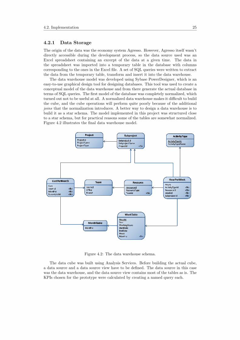
4.2.1 Data Storage

The origin of the data was the economy system Agresso. However, Agresso itself wasn’tdirectly accessible during the development process, so the data source used was anExcel spreadsheet containing an excerpt of the data at a given time. The data inthe spreadsheet was imported into a temporary table in the database with columnscorresponding to the ones in the Excel file. A set of SQL queries were written to extractthe data from the temporary table, transform and insert it into the data warehouse.

The data warehouse model was developed using Sybase PowerDesigner, which is aneasy-to-use graphical design tool for designing databases. This tool was used to create aconceptual model of the data warehouse and from there generate the actual database interms of SQL queries. The first model of the database was completely normalized, whichturned out not to be useful at all. A normalized data warehouse makes it difficult to buildthe cube, and the cube operations will perform quite poorly because of the additionaljoins that the normalization introduces. A better way to design a data warehouse is tobuild it as a star schema. The model implemented in this project was structured closeto a star schema, but for practical reasons some of the tables are somewhat normalized.Figure 4.2 illustrates the final data warehouse model.

Figure 4.2: The data warehouse schema.

The data cube was built using Analysis Services. Before building the actual cube,a data source and a data source view have to be defined. The data source in this casewas the data warehouse, and the data source view contains most of the tables as is. TheKPIs chosen for the prototype were calculated by creating a named query each.


4.2.2 Presentation

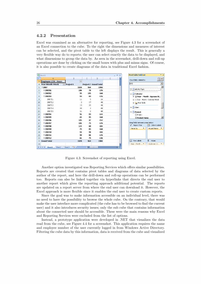
Excel was examined as an alternative for reporting, see Figure 4.3 for a screenshot ofan Excel connection to the cube. To the right the dimensions and measures of interestcan be selected, and the pivot table to the left displays the result. This is generally avery flexible way do to reports; the user can select exactly the data to be displayed, andwhat dimensions to group the data by. As seen in the screenshot, drill-down and roll-upoperations are done by clicking on the small boxes with plus and minus signs. Of course,it is also possible to create diagrams of the data in traditional Excel fashion.

Figure 4.3: Screenshot of reporting using Excel.

Another option investigated was Reporting Services which offers similar possibilities.Reports are created that contains pivot tables and diagrams of data selected by theauthor of the report, and here the drill-down and roll-up operations can be performedtoo. Reports can also be linked together via hyperlinks that directs the end user toanother report which gives the reporting approach additional potential. The reportsare updated on a report server from where the end user can download it. However, theExcel approach is more flexible since it enables the end user to create custom reports.

Since the goal was to make information accessible on an individual level, there wasno need to have the possibility to browse the whole cube. On the contrary, that wouldmake the user interface more complicated (the cube has to be browsed to find the currentuser) and it also introduces security issues; only the sub cube that contains informationabout the connected user should be accessible. These were the main reasons why Exceland Reporting Services were excluded from the list of options.

Instead, a prototype application were developed in .NET that visualizes the dataread from the cube, see Figure 4.4 for a screenshot. This application requires the nameand employee number of the user currently logged in from Windows Active Directory.Filtering the cube data by this information, data is received from the cube and visualized

4.3. Performance 27

as a graph. The user can specify which KPIs to display and the time period for whichto display the data.

Figure 4.4: Screenshot of the .NET application developed to present the data.

4.3 Performance

In order to measure and compare the performance, test data were generated and loadedinto the data warehouse and the cube. Query performance was tested for MDX queriesagainst the cube when it was configured for ROLAP and MOLAP respectively. Per-formance was also measured for SQL queries run against the data warehouse directly,without any optimizing techniques to see what difference it makes. A set of five testqueries were written in MDX, and a set of five corresponding SQL queries that gives thesame information were written for the data warehouse. The MDX and the SQL queriesdidn’t produce the exact same result depending on architecture differences. MDX isby nature multidimensional and the result set can be compared to a spreadsheet withcolumn and row labels, e.g. hours worked on rows and resource id on columns. TheSQL queries, at the other hand, produce tables which only has column labels. However,the information that can be interpreted from the data is the same.

The actual query performance were measured with the SQL Server Profiler, a toolused to log all events that occur during any operation on the database, with timestampand duration. The test was made by doing three implementations: (a) a test datagenerator; (b) a test executioner that loads the data warehouse and the cubes, and thenexecutes the test queries; and finally (c) a test result parser for the trace log files thatwere produced by the profiler.

When implementing the test data generator, the intention was to make the testdata look like real data, but without too much effort put on the small details. Given anumber of employees, a data file of the same format as the authentic data sheets wereto be generated. Every employee in the test data set work 40 hours a week, every weekof the year, distributed over randomly selected activity types and projects.

The first version of the generator wrote Excel files as output because the source


data were provided in this format. When the implementation was done and tested, theproblem with this approach was soon clear; when generating large sets of data, Excelcouldn’t handle it. Due to Microsoft’s specification1, Excel 2003 has a limit of 65 536rows per spreadsheet. It seemed like the next version, Excel 2007, could handle about1 000 000 rows, which would possibly be sufficient for the performance tests. However,this was not an option since Integration Services 2005 - which was the tool used forimporting Excel data into the database - doesn’t support the 2007 file format.

Another solution to the problem could be storing several sheets in one file, but thisidea didn’t seem very flexible and was not tested. Instead, the generator was rewrittento output plain text files. When the implementation was ready, 9 data sets of differentsizes were generated.

The test executioner used the same script that was written to import the real data.Every data set was imported into the data warehouse one by one, and for each data set,both a MOLAP and a ROLAP cube was loaded with the data. After the data set wasloaded into the cubes, each MDX query was executed 10 times on each cube and theSQL queries were executed 10 times each against the data warehouse.

Finally the test result parser was given the trace log files that were produced by theprofiler. In these log files, timestamps and durations of every operation was written.The log files were parsed and the average query duration for each combination of cube,query and data set (or query and data set for the non-cube tests) was calculated.

Details on the performance test such as the exact queries, the sizes of the data files,average durations, etc. can be found in Appendix A.

1See http://office.microsoft.com/en-us/excel/HP051992911033.aspx for details

5Conclusions

This chapter presents the conclusions reached while working on the project.The goals of the practical part, and how they were met in the resulting imple-mentation is discussed as well as the conclusions from the more theoreticalpart.

The need for multidimensional data analysis as a support for business decisions hasemerged during the last decades. The well accepted OLTP technology was not designedfor these tasks and therefore, the OLAP technology was developed as a solution. But dowe really need a technology like OLAP? Even though OLTP wasn’t designed for thesetasks, isn’t it possible to exploit the all-purpose relational database technology? Theshort answer is that it is quite possible to implement data cubes directly in a relationaldatabase engine without modifications, but it has its limitations.

5.1 Why OLAP?

One way to do cubing without OLAP is of course to write SQL queries that extracts theresult sets that is desired, and that contains the same data that would result from equiv-alent OLAP operations. This was done as a comparison during the performance testsof the project, see Appendix A for details. There are however some major drawbackswith this approach.

First of all, the performance would be unacceptable when the database is very largewith many relations involved, for example a database of a complex organisation thathold many years of historical data. The joins and aggregations required would slow downquery response time enormously, and this can clearly be seen in the test results. However,the tests were performed with realtime calculations, and the query response time couldbe optimized with materialized views or maybe some explicit indexing. At the otherhand, the queries were executed against the star schema shaped data warehouse, whichis filled with redundant data to minimize the number of joins required. To do the samequeries against a normalized data source would deteriorate performance. Anyhow, sincethe OLAP tools are specifically developed for these kind of queries, they are of courseoptimized for short query response times. Some of these optimizations take advantageof the read-mostly nature of OLAP models and can hardly be found in an all-purposerelational database engine.

Second, the reporting would be limited. A great advantage of OLAP tools is thatthe user view is multidimensional and the reporting is very flexible. The cube operatorproposed by Gray et al. is helpful to avoid the complex queries required to do all

30 Chapter 5. Conclusions

necessary aggregations, but it is still presented in relational form which in this contextis a limitation. OLAP is very flexible with both column and row labels, and even if it isnot so common, reporting in more than two dimensions is fully possible. Adding to thisthe drill-down and roll-up operations makes these kind of tools superior to relationaldatabases when it comes to analyzing data.

Of course, the need for multidimensional data analysis for a smaller organisationwith a limited database may not require all the extensive capacity of OLAP tools, whichoften are expensive even though there are open source alternatives for BI solutions aswell1. During the performance test, the largest data set tested was a 2 GB raw datafile imported to the data warehouse. This file contains weekly hour reports for 20 000employees during one year, about 9 000 000 rows of data. This is quite a lot of data,and the slowest query executed had a duration of about 25 seconds.

As an intellectual experiment we assume that a small to medium sized, local clothingstore wants to analyze their sales, and they sell about 1 product every minute in averageas long as they are not closed. This will result in 480 transactions a day, and if we assumethere are 50 weeks in a year, compensating for holidays, and each week containing 6working days, that will sum up to about 150 000 transactions during one year. Thisis not even close to the test data set mentioned above, and thus querying this data setwithout any OLAP tools or specific optimizations would not be a problem.

As stated above, OLAP is a requirement for large scale data analysis. Most recentresearch papers concerning data cubes and data warehouses seem to agree that ROLAPis the most suitable architecture for OLAP, and basically that was what Codd et al.stated in their white paper back in 1993. The benefit that MOLAP brings is betterperformance, but the question is if it is worth reduced flexibility. ROLAP is moreflexible than MOLAP in the sense that not all cells in the data cube has to be pre-aggregated, this is also an important aspect of the scalability of OLAP applications.When the number of dimensions increases the data explosion problem grows, primarilywith MOLAP, and at some point it becomes overwhelming.

However, there are researchers who still advocate MOLAP as the superior technologyand they are supported by some vendors, one of them being Microsoft, offering the usera choice between the two architectures in Analysis Services. Even if both options areavailable, the MOLAP is strongly recommended because of its increased performance [9].

The performance tests conducted during this project indicate that MOLAP indeedhas a better performance with Analysis Services, which is quite expected since aggre-gating data is a demanding task. However, I did expect that the difference betweenMOLAP and ROLAP would be greater. It would be interesting to do tests on morecomplex models of larger scale, especially models with many dimensions. If the perfor-mance gain coming from using MOLAP isn’t very large, then there is really no reasonto chose MOLAP. It also seems that there are many solutions for optimizing ROLAPperformance, and by using these, ROLAP can probably compete with MOLAP when itcomes to performance issues.

5.2 Restrictions and Limitations

The implementation was done in two different versions; one as an ASP.NET web page,and one as a .NET Windows application. The Windows application seemed to work

1Pentaho BI Suite is an example of a completely free, open source solution for BI,http://www.pentaho.com/

5.3. Future work 31

properly, but the ASP.NET web page could only be run in the development environ-ment since a problem with the Active Directory (AD) emerged. When the applicationwas launched on the intranet, the communication with the AD didn’t work and the ap-plication couldn’t receive the employee number needed to filter the data from AnalysisServices. One of the project goals was to make the information available on Sogeti’s in-tranet, but since there wasn’t enough time to fix the above problem, only the Windowsapplication was made available for download on the intranet.

In this implementation, the .NET application has full access to the data cube withoutrestrictions, and this could be considered a potential security risk. It is possible to setsecurity in the cube, but it would be quite complicated because there are lots of usersthat got to have access to the cube, and the information about them is stored in theWindows Active Directory (AD). Setting the security in the cube for each user wouldrequire some kind of connection between the AD and the cube, which most likely ispossible, but there was not enough time to investigate this option and therefore thewhole cube was made accessible with just one login, giving the responsibility of managingsecurity to the application prototype.

5.3 Future work

During this project I didn’t have direct access to Agresso, instead I received excerpts ofthe database stored as Excel spreadsheets. These spreadsheets were manually extractedfrom Agresso and then sent by e-mail. With these prerequisites, an automation ofthe updating process is complicated to implement. It is probably possible to triggerthe loading process when an e-mail with new data arrives, but it requires the Excelspreadsheet to have an exact structure in order to import the data correctly, and theemail has to be sent regularly when new data is available. Another option is thatsomebody manually starts the loading process every month, and makes sure that the datastructure is correct. This is how the loading process was done during the developmentof the prototype. The best option for a running system would however be direct accessto the data source.

The management of Sogeti Sverige AB has shown interest in the project, and by thetime my work was finished, a large scale project was initiated at a national level of thecompany to implement similar functionality on the intranet.

References

[1] S. Agarwal, R. Agrawal, P. Deshpande, A. Gupta, J. F. Naughton, R. Ramakrish-nan, and S. Sarawagi. On the Computation of Multidimensional Aggregates. InVLDB ’96: Proceedings of the 22th International Conference on Very Large DataBases, pages 506–521, San Francisco, CA, USA, 1996. Morgan Kaufmann Publish-ers Inc.

[2] S. Chaudhuri and U. Dayal. An Overview of Data Warehousing and OLAP Tech-nology. SIGMOD Rec., 26(1):65–74, 1997.

[3] E. F. Codd. A Relational Model of Data for Large Shared Data Banks. Commun.ACM, 13(6):377–387, 1970.

[4] E. F. Codd, S. B. Codd, and C. T. Salley. Providing OLAP to User-Analysts: AnIT Mandate. 1993.

[5] D. Comer. Ubiquitous B-Tree. ACM Comput. Surv., 11(2):121–137, 1979.

[6] P. M. Deshpande, K. Ramasamy, A. Shukla, and J. F. Naughton. Caching Multidi-mensional Queries Using Chunks. In SIGMOD ’98: Proceedings of the 1998 ACMSIGMOD international conference on Management of data, pages 259–270, NewYork, NY, USA, 1998. ACM.

[7] R. Elmasri and S. Navathe. Fundamentals of Database Systems. Addison-Wesley,2004.

[8] J. Gray, S. Chaudhuri, A. Bosworth, A. Layman, D. Reichart, M. Venkatrao, F. Pel-low, and H. Pirahesh. Data Cube: A Relational Aggregation Operator GeneralizingGroup-By, Cross-Tab, and Sub-Totals. Data Min. Knowl. Discov., 1(1):29–53, 1997.

[9] R. Jacobson and S. Misner. SQL Server 2005 Analysis Services Step by Step.Microsoft Press, Washington, 2006.

[10] MicroStrategy. The Case for Relational OLAP. 1995 .https://www.microstrategy.com/Solutions/5Styles/olap analysis.asp.

[11] S. Misner. SQL Server 2005 Reporting Services Step by Step. Microsoft Press,Washington, 2006.

[12] P. E. O’Neil and D. Quass. Improved Query Performance with Variant Indexes. InJoan Peckham, editor, SIGMOD Conference, pages 38–49. ACM Press, 1997.

[13] P. Turley, J. Kasprzak, S. Cameron, S. Iizuka, and P. Guzman. SQL Server 2005Integration Services Step by Step. Microsoft Press, Washington, 2007.

34 References

[14] K. Wu, E. J. Otoo, and A. Shoshani. A Performance Comparison of Bitmap Indexes.In CIKM ’01: Proceedings of the tenth international conference on Information andknowledge management, pages 559–561, New York, NY, USA, 2001. ACM.

[15] K. Wu, E. J. Otoo, and A. Shoshani. On the Performance of Bitmap Indices forHigh Cardinality Attributes. In Mario A. Nascimento, M. Tamer Ozsu, DonaldKossmann, Renee J. Miller, Jose A. Blakeley, and K. Bernhard Schiefer, editors,VLDB, pages 24–35. Morgan Kaufmann, 2004.

Appendix A

Performance Test Details

The performance tests were made with generated test data. 9 test data file were gen-erated based on a given number of employees, and for each employee, hour data weregenerated for each working day during one year. The data files were imported separatelyinto a data warehouse, and for each data set a MOLAP and a ROLAP cube were loaded.

To do the test, five different MDX queries and five corresponding SQL queries werewritten. The SQL queries return the same result as the MDX queries, but the result isnot exactly the same due to fundamental differences in the database models; the MDXqueries on the cubes returns a two-dimensional result set with both row and columnlabels while the SQL queries on the data warehouse returns ordinary relations with onlycolumn labels. However, the meaning of the resulting data is the same.

For every data set, the five MDX queries were run 10 times each on the two cubes,and the SQL queries were run 10 times on the data warehouse. SQL Server Profiler wasused to measure the duration of the queries, and the average durations were calculatedand are listed below.

The computer used for the performance testing was a virtual server running Win-dows Server 2003 R2, Standard edition. According to the Windows system, the virtualmachine was running on an Intel Pentium 4 2,8 GHz processor with 640 MB of RAM.

Table A.1 describes the 9 data sets that were generated. The number of employeesin each data set and the number of rows generated is provided.

Data Set # Employees Rows Generated

1 100 46 0422 1 000 442 2303 2 000 888 8414 5 000 2 218 4875 7 500 3 342 7436 10 000 4 468 8587 13 000 5 811 2948 16 500 7 351 3679 20 000 9 268 325

Table A.1: Test data sets used during performance testing

The disk size of each data file and the corresponding databases (MOLAP cube,ROLAP cube and data warehouse) is described in Table A.2. Note that the data storedin the data warehouse is often redundant due to its non-normalized structure. Projectnames and activity type names are examples of string data that is redundant and thereby

36 Appendix A. Performance Test Details

occupy much more space than required. This is probably the main reason why the cubesare far more compact than the data warehouse.

Data Set # Data File DW ROLAP Cube MOLAP Cube

1 10 285 18 560 2 233 2 7402 98 817 148 544 2 235 5 1913 198 591 296 021 2 256 9 8314 495 728 746 581 2 254 21 4345 746 897 1 106 176 2 275 35 2466 998 519 1 477 888 2 259 45 5117 1 298 472 1 921 408 2 302 66 7958 1 642 247 2 428 864 2 309 89 1309 2 070 770 3 069 760 2 304 112 842

Table A.2: Sizes in kB of the test data files, the data warehouse (DW) and the datacubes.

Table A.3 and Table A.4 list the query durations measured for the five MDX querieson the ROLAP and the MOLAP cube. The execution of queries 2 and 5 on data sets 5to 9 (the entries marked with -) gave rise to the following error during execution:

Memory error: While attempting to store a string, a string was found thatwas larger than the page size selected. The operation cannot be completed.

The queries were sent to the cube engine from a .NET application that was developedfor testing the performance. The problem seemed to arise when the result set was toolarge, it couldn’t be sent back to the application due to limitations on the page size.The result of this was that the durations from these erroneous queries were a lot shorterthan they were expected to be, considering the durations of queries with no errors. Theerroneous durations have been removed and are represented by zero in Figure A.1.

Data Set # Query 1 Query 2 Query 3 Query 4 Query 5

1 541 234 170 363 4662 1 145 1 024 196 319 3 2943 1 351 1 926 217 458 5 0834 2 175 18 375 313 773 24 3085 1 682 - 562 588 -6 1 879 - 516 616 -7 2 417 - 564 874 -8 2 808 - 712 696 -9 2 248 - 829 954 -

Table A.3: Average query durations for the ROLAP cube (µs).

The SQL queries were executed against the data warehouse in two modes; cachedand not cached. These results are listed in Table A.5 and Table A.6. As can be seen,the problem with large result sets was not an issue when querying the data warehouse.

Figure A.1 visualizes durations for the five MDX queries as well as the five SQLqueries. The reason for separating the data series and for putting the MDX and the SQLquery durations in different graphs becomes quite clear when looking at the magnitude;

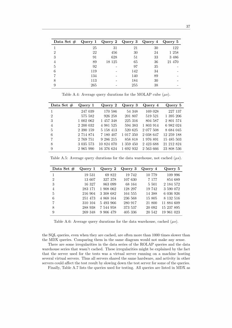
37


1 25 31 21 30 1222 22 456 30 24 1 2583 91 628 51 33 3 4864 89 18 125 65 36 21 4705 92 - 97 35 -6 119 - 142 34 -7 134 - 140 89 -8 113 - 184 30 -9 265 - 255 38 -

Table A.4: Average query durations for the MOLAP cube (µs).


1 247 039 170 586 54 348 169 028 227 1372 575 582 926 258 201 807 519 521 1 395 2063 1 002 062 1 457 348 225 316 804 587 2 801 5744 2 200 032 4 981 525 594 383 1 803 914 6 982 0245 2 390 159 5 158 413 520 625 2 077 508 8 684 0456 2 714 874 7 180 407 1 017 350 2 038 647 12 259 1887 2 769 751 9 286 215 858 818 1 976 891 15 485 5038 3 035 573 10 824 070 1 359 450 2 423 688 21 212 8249 2 965 990 16 376 624 1 692 932 2 563 666 23 808 536

Table A.5: Average query durations for the data warehouse, not cached (µs).


1 19 531 69 822 19 742 10 779 109 9962 13 607 327 378 107 630 7 177 854 6893 16 327 863 099 68 164 5 501 2 184 5724 283 171 1 908 062 128 297 19 742 3 590 0725 216 904 3 308 682 164 555 14 388 6 036 9266 251 473 4 868 164 236 568 15 805 8 132 5167 310 104 5 493 966 280 917 21 800 11 884 6098 288 938 7 544 958 373 537 20 092 15 237 8959 269 348 9 906 479 405 336 20 542 19 961 023

Table A.6: Average query durations for the data warehouse, cached (µs).

the SQL queries, even when they are cached, are often more than 1000 times slower thanthe MDX queries. Comparing them in the same diagram would not make any sense.

There are some irregularities in the data series of the ROLAP queries and the datawarehouse series that wasn’t cached. These irregularities might be explained by the factthat the server used for the tests was a virtual server running on a machine hostingseveral virtual servers. Thus all servers shared the same hardware, and activity in otherservers could affect the test result by slowing down the test server for some of the queries.

Finally, Table A.7 lists the queries used for testing. All queries are listed in MDX as


well as SQL, and a short description explains the meaning of the queries.

39

Figure A.1: Diagrams visualizing query durations for both the cube and the data ware-house.


MD

XSQ

LM

eanin

g

4SE

LE

CT

SE

LE

CT

Week

Table.M

onth

Id,

‘For

each

month

durin

g2007,select

{[R

esource].[R

esource

Id].[1

]}SU

M(B

Hours)

/SU

M(W

eekTable.W

ork

ingH

ours)

bonus

quotien

tfo

rem

plo

yee

with

id1.’

ON

CO

LU

MN

S,

FR

OM

Bonus,

Week

Table

{[C

alen

dar].[M

onth

].[200701]:

WH

ER

EB

onus.W

eekId

=W

eekTable.W

eekId

AN

D[C

alen

dar].[M

onth

].[200712]}

Bonus.R

esourceId

=1

AN

DO

NR

OW

SW

eekTable.M

onth

Id>

=200701

AN

DFR

OM

[Kobi]

Week

Table.M

onth

Id<

200801

WH

ER

E[B

onus];

GR

OU

PB

YR

esourceId

,W

eekTable.M

onth

Id;

5SE

LE

CT

SE

LE

CT

Reso

urceId

,M

onth

Id,

‘Select

bonus

quotien

tfo

rev

eryem

plo

yee

{[R

esource].[R

esource

Id].m

embers}

SU

M(B

Hours)

/SU

M(W

eekTable.W

ork

ingH

ours)

each

month

durin

g2007.’

ON

CO

LU

MN

S,

FR

OM

Bonus,

Week

Table

{[C

alen

dar].[M

onth

].[200701]:

WH

ER

EB

onus.W

eekId

=W

eekTableW

eekId

[Calen

dar].[M

onth

].[200712]}

GR

OU

PB

YR

esourceId

,M

onth

Id;

ON

RO

WS

FR

OM

[Kobi]

WH

ER

E[B

onus];

Table

A.7:

MD

Xand

theircorresponding

SQL

queriesused

duringthe

performance

testing(continued).

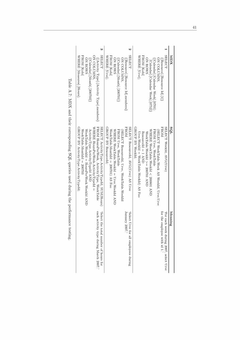
41

MD

XSQ

LM

eanin

g

1SE

LE

CT

SE

LE

CT

Week

Id,AV

G(U

rve)

‘For

each

week

durin

g2007,select

Urv

e{[R

esource].[R

esource

Id].[1

]}FR

OM

for

the

emplo

yee

with

id1.’

ON

CO

LU

MN

S,

(SE

LE

CT

Week

Table.W

eekA

SW

eekId

,U

rve.U

rve

{[C

alen

dar].[C

alen

dar

Week

].[0701]:

FR

OM

Urv

e,W

eekTable

[Calen

dar].[C

alen

dar

Week

].[0752]}

WH

ER

EW

eekTable.W

eekId

<200801

AN

DO

NR

OW

SW

eekTable.W

eekId

>=

200701

AN

DFR

OM

[Kobi]

Reso

urceId

=1

AN

DW

HE

RE

[Urv

e];U

rve.W

eekId

=W

eekTable.W

eekId

)A

SFoo

GR

OU

PB

YW

eekId

;

2SE

LE

CT

SE

LE

CT

Reso

urceId

,AV

G(U

rve)

AS

Urv

e‘S

electU

rve

for

all

emplo

yees

durin

g{[R

esource].[R

esource

Id].m

embers}

FR

OM

January

2007.’

ON

CO

LU

MN

S,

(SE

LE

CT

Reso

urceId

,U

rve,

Week

Table.W

eekId

{[C

alen

dar].[M

onth

].[200701]}

FR

OM

Urv

e,W

eekTable

ON

RO

WS

WH

ER

EW

eekTable.W

eekId

=U

rve.W

eekId

AN

DFR

OM

[Kobi]

Week

Table.M

onth

Id=

200701)

AS

Foo

WH

ER

E[U

rve];

GR

OU

PB

YR

esourceId

;

3SE

LE

CT

SE

LE

CT

Activ

ityT

ype.A

ctivity

TypeId

,SU

M(H

ours)

‘Select

the

tota

lnum

ber

ofhours

for

{[A

ctivity

Type].[A

ctivity

Type].m

embers}

FR

OM

HoursP

erWeek

,A

ctivity

Type,

Week

Table

each

activ

ityty

pe

durin

gM

arch

2007.’

ON

CO

LU

MN

S,

WH

ER

EH

oursP

erWeek

.Activ

ityT

ypeId

={[C

alen

dar].[M

onth

].[200703]}

Activ

ityT

ype.A

ctivity

TypeId

AN

DO

NR

OW

SW

eekTable.W

eekId

=H

oursP

erWeek

.Week

IdA

ND

FR

OM

[Kobi]

Week

Table.M

onth

Id=

200703

WH

ER

E[M

easu

res].[Hours];

GR

OU

PB

YA

ctivity

Type.A

ctivity

TypeId

;

Table

A.7:

MD

Xand

theircorresponding

SQL

queriesused

duringthe

performance

testing.

Appendix B

Glossary

1NFAbbreviation of First Normal Form.

2NFAbbreviation of Second Normal Form.

3NFAbbreviation of Third Normal Form.

– A –

AggregationApplying an operator, for example sumor average, on all values in a data setis called aggregating. Aggregations areoften applied on a data set in combina-tion with the group by operator.

AgressoAgresso is a commercial business andeconomy system used by Sogeti.

Analysis ServicesA tool for building data cubes andanalysing data, a component ofMicrosoft SQL Server.

– B –

BIAbbreviation of Business Intelligence.Term referring to a technology used togather and analyze data in order to findwhat factors are affecting a business.

– C –

Candidate KeyAny key of a relational schema.

CardinalityThe cardinality of an attribute is thenumber of values in the domain asso-ciated with that specific attribute. Forexample, a relation with the attributegender would have a cardinality of 2since possible values are male and fe-male.

Composite KeyA key that consists of multiple at-tributes.

44 Appendix B. Glossary

– D –

Data CubeA database model used for analysingdata multidimensionally.

Data MiningTerm describing tools used to findtrends and patterns in large data sets.

Data WarehouseA central data storage used as a base forbuilding data cubes and do data mining.The data in a data warehouse is oftencollected from multiple, heterogeneousdata sources.

DBMSAbbreviation of DataBase Manage-ment System. Software that managesdatabases and transactions.

Dimension HierarchyA division in granularity levels of adimension. For example, a typi-cal time dimension hierarchy containsyears, months and days.

Dimension TableA database table that contains dimen-sion data, i.e. data that is used to groupmeasures.

DomainThe set of values that can be applied toa certain attribute.

Drill-downOperation on a data cube that traversesa dimension hierarchy down towards afiner granularity.

DSSAbbreviation of Decision Support Sys-tem. A computer system designed tohelp making decisions based on givenfacts.

– E –

ETLAbbreviation of Extract, Transform andLoad. Term describing the processof collecting data from multiple datasources and load it into a data ware-house.

– F –

Fact TableA database table that contains mea-sures and references to dimension ta-bles.

Foreign keyA foreign key in a relation is a set ofattributes that references a primary keyin another relation; that is, the values ofthe foreign key attributes must be foundin the referenced table.

– G –

GranularityLevel of detail of data in the data cube.The data in the data warehouse deter-mines the finest level of granularity ofthe cube, aggregations on this data cre-ates higher levels of granularity.

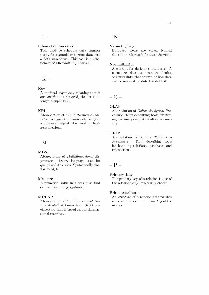
45

– I –

Integration ServicesTool used to schedule data transfertasks, for example importing data intoa data warehouse. This tool is a com-ponent of Microsoft SQL Server.

– K –

KeyA minimal super key, meaning that ifone attribute is removed, the set is nolonger a super key.

KPIAbbreviation of Key Performance Indi-cator. A figure to measure efficiency ina business, helpful when making busi-ness decisions.

– M –

MDXAbbreviation of Multidimensional Ex-pression. Query language used forquerying data cubes. Syntactically sim-ilar to SQL.

MeasureA numerical value in a data cube thatcan be used in aggregations.

MOLAPAbbreviation of Multidimensional On-line Analytical Processing. OLAP ar-chitecture that is based on multidimen-sional matrices.

– N –

Named QueryDatabase views are called NamedQueries in Microsoft Analysis Services.

NormalizationA concept for designing databases. Anormalized database has a set of rules,or constraints, that determine how datacan be inserted, updated or deleted.

– O –

OLAPAbbreviation of Online Analytical Pro-cessing. Term describing tools for stor-ing and analysing data multidimension-ally.

OLTPAbbreviation of Online TransactionProcessing. Term describing toolsfor handling relational databases andtransactions.

– P –

Primary KeyThe primary key of a relation is one ofthe relations keys, arbitrarily chosen.

Prime AttributeAn attribute of a relation schema thatis member of some candidate key of therelation.

46 Appendix B. Glossary

– Q –

QueryA text string sent to a DBMS in orderto modify or read from a database, forexample update, receive or insert data.

– R –

RDBMSAbbreviation of Relational DataBaseManagement System. Software thatmanages relational databases and trans-actions.

ROLAPAbbreviation of Relational Online An-alytical Processing. OLAP architecturethat is based on a relational database.

Roll-upOperation on a data cube that traversesa dimension hierarchy up towards acoarser granularity.

– S –

Secondary KeyAll keys in a relation that is not chosento be the primary key.

Snowflake SchemaA way to structure data warehouses.The snowflake schema is a star schemathat has been normalized.

Star SchemaA way to structure data warehouseswith a fact table in the middle, refer-encing surrounding dimension tables.

Super KeyA set of attributes that functionally de-termines all other attributes in a rela-tion.

SQLAbbreviation of Structured Query Lan-guage. Language used for querying re-lational databases.

– T –

TupleAn ordered list of values, which are el-ements of a specific domain.

– U –

URVEAbbreviation of Utilisation Rate Vaca-tion Excluded. One of the KPIs usedduring the project.

Business Intelligence: Multidimensional Data Analysis · Business Intelligence: Multidimensional...

Documents

Transcript of Business Intelligence: Multidimensional Data Analysis · Business Intelligence: Multidimensional...