Business Cycles and Macroeconomic Policy Coordination in ...

Business Cycles and Macroeconomic Policy

Coordination in Mercosur

Jose Marıa FanelliCEDES

Martın Gonzalez-Rozada∗

Escuela de Negocios

Universidad Torcuato Di Tella

March, 2004

Abstract: The paper analyzes cyclical comovements in the Mercosur area differentiating idiosyncraticfrom common shocks. In the Mercosur (or any region for that matter) shocks can be country-specific,affecting only one country or a specific set of countries (for example, a weather-related shock, adomestic policy shock); or they can be common to the entire region (for example, a change in theconditions in international capital markets or a world recession). Propagation mechanisms, in turn,are important because a shock that was initially country-specific, originating in one country, mighteventually spillover to others. We build on the unobserved component approach to decompose theMercosur countries’ real GDP (seasonally adjusted) fluctuations into these three components andcompare them with previous results. The main findings in the paper are: first, common factorsoriginating in impulses stemming from changes in investor’s sentiment are relevant to explainingregional output comovements and the spillover effects between neighbors are significant. Second,volatility matters, and matters especially in the case of recent regional agreements. Supply shocks inMercosur countries tend to be larger than in the US and European countries. Third, finance mattersfor both volatility and output/price dynamics. Accelerator effects may be important in explainingsome features of the output/price dynamics that the standard models based on vector autoregressiontechniques are unable to account for.

Key-Words: Business cycle, Comovement, Mercosur, OCA, Policy coordination, Unobserved com-ponents, VAR, Volatility.JEL Classification: C32, E32, F02.

∗Jose Marıa Fanelli, CEDES, Sanchez de Bustamente 27, (1173) Buenos Aires, Argentina, Phone: (54-11) 4861-2126, [email protected]. Martın Gonzalez-Rozada, Universidad Torcuato Di Tella, Minones 2177,(C1428ATG) Buenos Aires, Argentina, Phone: (54-11) 4784-0080, [email protected]. We gratefully acknowl-edge the financial support of the International Development Research Center and research assistance by ArielGeandet. The second author thanks the CIF (Centro de Investigacion en Finanzas) at Universidad TorcuatoDi Tella for support.

1 Introduction

The main purpose of this paper is to analyze aggregate fluctuations and cyclical comovements

in the Mercosur area, as well as to draw conclusions on macroeconomic policy coordination.1

Our primary concern will be to characterize the fluctuations in GDP. We basically follow the

literature on optimum currency areas (OCA) and exchange-rate-regime choice. Therefore, the

issues that we discuss here are to a great extent those treated in that literature: the degree of

symmetry of the business cycles, the identification of the sources of shocks, volatility, and the

interactions between the cyclical movements of output and prices.2

Our treatment of cyclical fluctuations, nonetheless, departs from the literature insofar as

the emphasis we give to certain factors. This is basically due to the fact that the Mercosur

presents a series of particularities that must be incorporated into the analysis. The most relevant

are: first, that the Mercosur is a relatively recent regional integration agreement in which the

degree of economic and trade integration is still low; second, its members are instability-prone

medium-income countries and some are highly dollarized; and third, the countries have been hit

by sizable shocks in the last five years and this has been detrimental to the integration process.

In our view, the particularities of the Mercosur macroeconomic setting indicate that focus-

ing exclusively on the problem of the symmetry of business cycles may not be the best research

strategy. In the OCA-inspired studies on the cycle, the identification of common shocks and of

the degree of harmony in the adjustment process play prominent roles because of their primary

interest on the cost-and-benefit analysis of renouncing the independence of monetary policy.

In the case of Mercosur, the problem of relinquishing monetary policy in favor of a common

one with the members of an eventual monetary union is not the most pressing issue of the day.

The key macroeconomic policy question poses whether regional actions can be taken to reduce

the volatility of some variables—the real bilateral exchange rate in the first place— thereby

facilitating the process of integration. A closely related question considers what institutional

framework at the regional level and what domestic policy regimes can best support the coordi-

1The findings on the cycle that we will present are the result of an ongoing research project on macroeconomic

policy coordination undertaken by the Mercosur Research Network. At a previous stage of the project we

analyzed the constraints from the structure of intraregional trade in the region, the behavior of prices, and some

of the institutional issues involved. See Fanelli, Gonzalez-Rozada, and Keifman (2001).2In Fanelli (2001) we discussed the relationship between this literature and our research project.

2

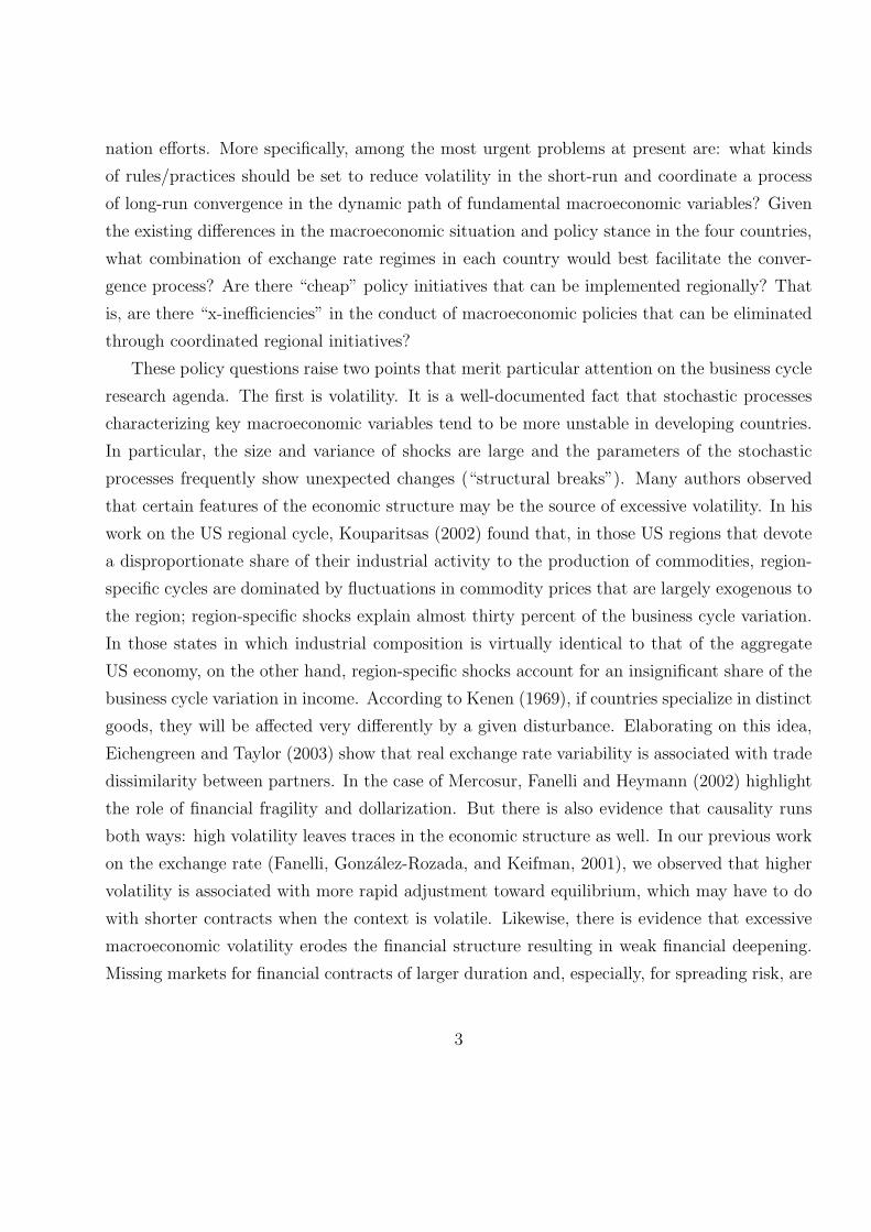
nation efforts. More specifically, among the most urgent problems at present are: what kinds

of rules/practices should be set to reduce volatility in the short-run and coordinate a process

of long-run convergence in the dynamic path of fundamental macroeconomic variables? Given

the existing differences in the macroeconomic situation and policy stance in the four countries,

what combination of exchange rate regimes in each country would best facilitate the conver-

gence process? Are there “cheap” policy initiatives that can be implemented regionally? That

is, are there “x-inefficiencies” in the conduct of macroeconomic policies that can be eliminated

through coordinated regional initiatives?

These policy questions raise two points that merit particular attention on the business cycle

research agenda. The first is volatility. It is a well-documented fact that stochastic processes

characterizing key macroeconomic variables tend to be more unstable in developing countries.

In particular, the size and variance of shocks are large and the parameters of the stochastic

processes frequently show unexpected changes (“structural breaks”). Many authors observed

that certain features of the economic structure may be the source of excessive volatility. In his

work on the US regional cycle, Kouparitsas (2002) found that, in those US regions that devote

a disproportionate share of their industrial activity to the production of commodities, region-

specific cycles are dominated by fluctuations in commodity prices that are largely exogenous to

the region; region-specific shocks explain almost thirty percent of the business cycle variation.

In those states in which industrial composition is virtually identical to that of the aggregate

US economy, on the other hand, region-specific shocks account for an insignificant share of the

business cycle variation in income. According to Kenen (1969), if countries specialize in distinct

goods, they will be affected very differently by a given disturbance. Elaborating on this idea,

Eichengreen and Taylor (2003) show that real exchange rate variability is associated with trade

dissimilarity between partners. In the case of Mercosur, Fanelli and Heymann (2002) highlight

the role of financial fragility and dollarization. But there is also evidence that causality runs

both ways: high volatility leaves traces in the economic structure as well. In our previous work

on the exchange rate (Fanelli, Gonzalez-Rozada, and Keifman, 2001), we observed that higher

volatility is associated with more rapid adjustment toward equilibrium, which may have to do

with shorter contracts when the context is volatile. Likewise, there is evidence that excessive

macroeconomic volatility erodes the financial structure resulting in weak financial deepening.

Missing markets for financial contracts of larger duration and, especially, for spreading risk, are

3

a canonical feature of the region. This suggests that financial aspects should play a significant

role in the analysis of shocks and propagation mechanisms.

The second point that deserves attention on the research agenda is the relationship be-

tween idiosyncratic and common (regional) cycles. When the degree of integration is low and

the market structure has significant missing markets, one would expect—ceteris paribus—a

low correlation of business cycles. However, a low correlation of cyclical movements does not

mean that there are no coordination opportunities to exploit. The countries could still reduce

macroeconomic volatility by implementing mechanisms to exchange idiosyncratic risks. The

implementation of these mechanisms should improve both macroeconomic stability and wel-

fare because it would expand trading opportunities and permit exchanging risks that could

not otherwise be exchanged insofar as the international markets for transacting those risks are

clearly missing. For these mechanisms to be designed and implemented, it is critical to fully

comprehend the relationship between common and idiosyncratic cycles and to identify regional

propagation mechanisms within a unified methodological framework

The issues that we study in this paper are closely related with these two points. The

rest of the paper is organized as follows. The second section presents the stylized facts of

output fluctuations in Mercosur. The purpose is twofold: to present empirical evidence and to

motivate the analysis. The third reviews and discusses the approaches used in previous studies

on cyclical comovement in Mercosur and proposes some innovations for addressing the issues

raised in the introduction and in the section dealing with stylized facts. The fourth section

presents the estimates of a VAR model for identifying supply and demand shocks based on the

Blanchard and Quah (1989) methodology (BQ hereafter) and examines the weaknesses of this

approach to account for price/output dynamics in Mercosur. The fifth section presents estimates

of the common and idiosyncratic cycles in Mercosur. We apply the unobserved component

methodology developed by Watson (1986) and Kouparitsas (2002) to identify the common

(regional) and idiosyncratic (national) components of cyclical fluctuations in the region. We

also investigate the relationship between the estimated common cycle and changes in financial

conditions. The sixth section concludes the paper.

4

2 Cyclical Comovements in Mercosur: the Stylized Facts

Identifying the shocks that affect a specific economic area—a country, the sub-region of a coun-

try, or an aggregate of countries in a regional agreement—and characterizing the propagation

mechanisms that operate are two key purposes of business cycle studies. As was mentioned

above, our analysis will focus on the regional dimension of business cycles rather than the

national level. Our primary concern is to characterize fluctuations and comovements in the

GDP.3 We will measure the size of shocks affecting the product, its volatility, and the speed of

adjustment toward equilibrium after a disturbance has occurred. On these bases we will assess

the degree of business cycle comovement across Mercosur countries, which implies identifying

common sources of disturbances, country-specific shocks, and cross-country spillover effects.

The study of these factors is very demanding on both analytical and empirical grounds.

The full specification of the structural model calls for a knowledge of the economic, policy,

and institutional factors that often go well beyond the state of the art in developing-country

macroeconomics. However, even if we were able to specify correctly the stochastic structural

model at the analytical level, the identification of its parameters usually calls for a knowledge

of the data generating process that is inconsistent with the quantity and quality of the data

available in the countries under study. Given these constraints, we will adopt a heterodox

strategy and will approach the problem from different perspectives. We will first characterize the

most important stylized facts and, then, try different approaches to model shocks, comovements,

and propagation mechanisms. By using different models and procedures we hope to highlight

different factors that we regrettably cannot show within a unified framework.

The first row of Table 1, Panel A, reports the average quarterly growth rates of the three

countries under analysis from 1980 to the present. It is clear that the rate of growth of Mercosur

countries has been very low in the last two decades. Although Brazil exhibits the highest growth

rate, its case is the most striking because Brazil was considered a “miracle” of high growth in

the post-war period. It is easy to anticipate, then, that the popularity of Mercosur and the

political will to deepen integration will be strongly influenced by the ability of the agreement to

contribute to restoring and sustaining growth. Panel B of Table 1 indicates that no substantial

differences exist between the pre- and post-Mercosur periods.4 Only Argentina shows a higher

3Owing to data availability, we do not include Paraguay in the analysis.4To be sure, we are describing the data and do not intend to imply any causal relationship between regional

5

growth rate, but its recovery in the nineties proved to be unsustainable.

A second apparent feature is the high volatility the three countries have experienced, al-

though it is much more marked in Argentina and Uruguay. The three countries exhibit a fall

in the standard deviation of GDP growth rate in the period that follows the establishment of

the agreement, but the differences between the two periods are far from striking. The wide gap

that still exists between the observed maximum and minimum values of the growth rate reveals

that the degree of instability is still too high. We must take into account, nonetheless, that the

most important achievement regarding volatility in the nineties does not appear in the table:

the generalized reduction in the mean and standard deviation of the inflation rate in the four

countries (See Fanelli, Gonzalez-Rozada, and Keifman, 2001). This represents an important

asset regarding the necessary conditions for macroeconomic policy coordination.

TABLE 1 about here

A natural first step to assess the degree of comovement of business cycles at the regional

level is to calculate the correlation between domestic business cycles, where “business cycle” is

defined as the residual left once the Hodrick-Prescott (H-P) trend has been removed.5 In this

context, a high correlation suggests the existence of common sources of and similar responses

to shocks. If the correlation is low, however, it may be due either to differing perturbations

and/or different responses to shocks. Table 2 shows that contemporaneous correlations between

Argentina and Brazil are low, while Uruguay experiences a larger degree of comovement with the

other members. The value of the coefficients indicates that the strongest comovement occurs

between Argentina and Uruguay. If we consider that the US is a well-developed monetary

union, we can use the value of the correlation coefficients between US regions as a standard

for comparison. According to the evidence in Kouparitsas (2002) the minimum value of the

correlation coefficient is 0.51 and the mean is 0.78. It is apparent that the degree of comovement

in Mercosur is much weaker. This suggests that common sources of disturbances are weak

and/or that the responses to common shocks are dissimilar. Regarding the latter, we should

consider that—with the possible exception of the third quarter 94/fourth quarter 98 period

integration and growth; to do so we would have to control for other factors, such as external financial shocks

and domestic structural reforms.5We have also used the Baxter-King filter to extract the trend (Baxter and King, 1995) but the results do

not differ significantly. Hence, we have not reported them here.

6

where Argentina and Brasil both had fixed exchange rates—the exchange rate regimes and,

hence, policy responses presented substantial differences in the period under analysis.

TABLE 2 about here

A contemporaneous correlation, however, does not permit the evaluation of persistence and

lead relationships. We can obtain a better knowledge of regional dynamics by computing lead

coefficients between these variables, that is, the correlation between output residuals6 at time

t and at time t + k, where k is a positive integer. Table 3 shows the value of the coefficients

for k = 1 and k = 4. Coefficients close to one indicate highly persistent cyclical fluctuations

while coefficients close to zero indicate very little persistence. Own-lead correlation coefficients

reveal a moderate degree of persistence with Brazil showing the lowest value. This suggests

that there is less inertia in the adjustment process, which is consistent with the findings on real

exchange rate in our previous work: the length of the periods of departure from trend after the

occurrence of a shock is shorter in these economies (Fanelli, Gonzalez-Rozada, and Keifman,

2001). In the case of US regions, for example, there are no own-lead coefficients below 0.9.

TABLE 3 about here

The effects of disturbances may be transmitted across countries via trade, productive, and

financial channels. If lead correlations are high relative to contemporaneous correlations, this

is an indication that there may be relevant propagation mechanisms at work. The linkages of

Uruguay with the other two partners are the most striking in this regard. The correlation be-

tween Argentine output residual at time t and Uruguayan output residual at t+1 is higher than

the contemporaneous correlation between these two variables and the coefficient corresponding

to Argentina at time t and Uruguay at time t+4 is only slightly lower. Something similar occurs

with the relationship between Uruguay and Brazil. The Brazilian(t) vs. Uruguayan(t + 1) and

the Brazilian(t) vs. Uruguayan(t + 4) correlation coefficients are 0.37 and 0.40, respectively.

Both are higher than the contemporaneous correlations (see Table 2). This means that both

the Argentine and the Brazilian cycle leads the Uruguayan cycle and that the value of the lead

coefficient does not decay very much over time (indeed, it increases in the case of Brazil). It is

6We use the term “output residuals” to indicate the deviations of output from its H-P trend.

7

interesting that the value of the four-lead correlation coefficients linking Uruguay with Brazil

and Argentina are higher than the Uruguayan own-lead correlation coefficient.

The correlations between Brazil and Argentina do not reveal strong lead relations but note

that the value of the coefficient of Brazil(t) vs. Brazil(t + 4) is similar to the coefficient of

Argentina(t) vs. Brazil(t + 4). The value of the latter is identical to the value of the one lead

coefficient between output residuals of Argentina and Brazil. It seems, on the other hand, that

neither Brazil nor Uruguay leads Argentina.

We can obtain a broader and synthetic view of the dynamic relationships between these

variables by plotting the cross-correlations. Figure 1 shows business cycle correlations between

one country output residual at time t = 0 and output residual at time t = k in the others,

for various k > 0. Two features stand out. First, Argentina and Brazil tend to lead Uruguay.

The correlation corresponding to different leads is positive and does not decay quickly. Second,

the values of the correlation coefficients linking different leads of Argentina’s output residuals

with an impulse originating in Brazil at time t = 0 are low and decay quickly (Panel B), and

a similar pattern of behavior is observed between Argentina at t = 0 and Brazil at t = k > 0

(Panel A).

FIGURE 1 about here

A drawback of assessing comovement on the basis of cross-correlations is that it only allows

for a rudimentary identification of the sources of shocks. To improve identification we will have

to apply more complex methods and make more audacious assumptions, which entails making

hypotheses about the interactions between shocks to output and prices. It may be useful, then,

to take a preliminary look at the dynamic linkages between prices and quantities.

Price residuals are measured as the deviation of the natural logarithm of a price index from

its H-P trend. Figure 2 displays the cross-correlation corresponding to price-output residuals.

We use two price indices, the “combined” index and the wholesale or producer index. The

combined index blends consumer and producer prices with equal weights and it is intended to

be a proxy for the implicit deflator of GDP. Panel A in Figure 2 displays the business cycle

correlations between combined prices at t = 0 and output at t = k for different values of k.

The shape of the curve indicates that there is an inverse relationship in the short run in the

three countries under analysis. Whenever there is a movement above trend in prices, there is a

8

movement below trend in output. The correlation turns positive, nonetheless, as time elapses.

Brazil shows the most rapid reversion in the sign of the correlation coefficient. This seems to be

counterintuitive. According to the literature, this relationship should be positive in the short

run and negative in the long run as demand impulses are stronger than supply forces in the

short run, with the sign of the correlation reversed as time elapses because of the dominance of

supply effects in the long run.

FIGURE 2 about here

In the Mercosur context, however, this fact is not as striking as it may seem at first glance. In

the region, prices tend to be above their trend under two basic circumstances. First, a demand

shock (because of monetary or fiscal impulses) creates extra inflationary pressures and output

expansion. As a consequence, when the impulse originates in a demand shock, we would expect

the response to take the form of a positive correlation between output and price residuals.

Second, upward deviations in prices also occur when the domestic currency depreciates, usually

to compensate for an external shock. The upward pressure on prices originates in the fact that

pass-through coefficients tend to be high in the region. But unlike the case of demand shocks,

real depreciation usually has contractionary effects on output; this is a well-documented fact in

the region, particularly in the case of Uruguay and Argentina. Hence, when an external shock

occurs (a “supply” shock) one would expect a negative correlation between prices and output

residuals. Historically, the most frequent external disturbances are supply shocks originating on

the trade side (variations in the terms of trade, oil shocks, or changes in the parity between the

main reserve currencies). In the last two decades, nonetheless, changes in financial conditions

became a primary source of shocks, hand in hand with the increase in capital flows. Under

these new circumstances, swings in market sentiment usually induce changes in the supply of

external funds and the country risk premium. Since “sudden stops” (Calvo and Reinhardt,

1999) create recessionary forces and upward pressures on the real exchange rate, this kind of

financial shock should also result in a negative correlation between output and price residuals.

In sum, the plot in Panel A suggests that supply/financial shocks dominate demand shocks

as a source of short-run disturbances. In the three countries, supply and financial impulses

seem to drive price-output responses in the short run. When we examine longer time horizons,

nonetheless, this counter-cyclical pattern weakens in the case of Brazil and persists in the case

9

of Argentina. This differential pattern may reflect the distinct responses to shocks that occur

in different financial settings, as we will discuss below.

We also have data on the price-output comovement in the case of industry. Panel B displays

output-price correlations using industrial production and producer prices to measure residuals.

The graph confirms the impression that a negative correlation exists between cyclical movements

of output and price residuals in the short run in the case of Argentina but disconfirms this

impression for Brazil. The reversion in sign may correspond to tradable sectors that are more

responsive to price signals than non-tradable sectors, which are more heavily represented in the

GDP index. Panels C and D show the responses of prices to output impulses. The correlogram

indicates that there is a consistent negative correlation between output residuals in t = 0 and

various leads of price residuals.

In the preceding paragraphs we advanced some conjectures about the behavior of the real

exchange rate vis-a-vis output residuals. Let us examine the cross-correlation linking real

exchange rate variations with output residuals (see Figure 3). The first panel in Figure 3

indicates that the contemporaneous correlation between the real exchange rate (measured in

natural logarithm) and cyclical movements in output is negative. That is, whenever the real

exchange rate increases (i.e. the country becomes more competitive), real output tends to fall

below its trend in the ensuing periods. In the case of Uruguay and Argentina the correlation

remains negative for several quarters after the change in the real exchange rate takes place. In

the case of Brazil, to the contrary, the correlation coefficient soon becomes positive, indicating

that real depreciation is less contractionary. This provides additional evidence in favor of the

hypothesis that Brazilian producers respond more quickly to relative prices. It could also

be the case that more Brazilian firms on the verge of international competitiveness become

internationally competitive immediately following real depreciation. Another factor that may

have a bearing on this adjustment dynamics is the lower degree of dollarization in the Brazilian

financial system. Under imperfect financial markets, variations in the real exchange rate affect

the financial position of firms and banks when currency mismatches exist (see Bebczuk, Fanelli,

and Pradelli 2002 for the Argentinian case). It seems sensible to assume, then, that via financial

accelerator effects, higher dollarization strengthens the negative effects of increases in the real

exchange on output.

FIGURE 3 about here

10

To further investigate this latter hypothesis, Panel B displays the evolution of industrial

output following an alteration in the real exchange rate. Many more firms are exposed to

external competition in the industrial sector than in the economy as a whole. Consequently,

one would expect the real depreciation to benefit industry not only because industrial firms

produce tradables but because the incidence of the currency mismatch effect should be weaker

in the case of these firms. In effect, tradable firms will see the value of both their assets and their

dollarized liabilities moving in the same direction after depreciation, while non-tradable firms

holding dollarized liabilities will experience a reduction in their net worth. Panel B in Figure 3

plots the correlations between the real exchange rate at t = 0 and the leads of industrial output

residuals. In the case of Brazil, which is the least dollarized economy, these correlations rapidly

turn positive as t increases. In Argentina, to the contrary, it takes three quarters for output

residuals to become positive after real depreciation occurs. Note, however, that the high degree

of persistence shown by the negative comovement between GDP residuals and real depreciation

that we found in Panel A has disappeared in Panel B. This is consistent with our hypotheses

about the roles of dollarization and competitiveness.

3 Modeling cyclical comovements and shocks

The great majority of the studies analyzing aggregate fluctuations and the problem of monetary

cooperation in Mercosur follows the OCA literature and concentrates on the analysis of the

synchronicity of business cycles. The degree of sophistication of the studies varies greatly,

depending on the methodology and the data utilized, but there are essentially two approaches.

One is based on panel data techniques and the other on time series methods.

Eichengreen (1998) and Eichengreen and Taylor (2003) are important studies using cross

country data and panel data techniques to address the question of whether Mercosur needs a

single currency and, more generally, what the monetary consequences of a Free Trade Area of the

Americas would be. To answer these questions they build on the theory of OCA (augmented to

include a role for regionalism) and derive a model of the determinants of exchange rate outcomes.

In their view, to assess the conditions for monetary cooperation it is necessary to investigate

the determinants of bilateral exchange rate volatility. The approach is ambitious because they

include all of the factors the OCA literature highlighted as relevant in the equation explaining

11

exchange rate volatility. The main conclusion on Mercosur is that no important economic

impediments exist for monetary cooperation and that the lack of political will may be the most

important obstacle: “The failure to engage in monetary cooperation in MERCOSUR is not

obviously a function of economic variables. The countries do not have unusual size, trade,

composition, or other economic characteristics that militate against monetary cooperation; in

this respect they are reasonably similar to the EU. Rather, the sources of the cooperation deficit

lie elsewhere” (Eichengreen and Taylor, 2003 p. 25). The authors provide evidence that higher

synchronicity of the business cycle is associated with lower volatility of the bilateral rate. From

the perspective of the stylized facts that we discussed above, Eichengreen and Taylor (2003)

offer two valuable features. First, they show that more recent regional trade agreements tend

to be more volatile. Second, they recognize that the OCA approach, which focuses on the

current account, may have some limitations in the context of Latin America—and particularly

in Mercosur—because the capital account matters in this region and finance may be more

important than trade to explain exchange rate fluctuations. Consequently, they extend the

framework to take into account the financial characteristics and external vulnerabilities of the

regional members. These studies, nonetheless, have serious drawbacks in the treatment of cycles.

Data availability and the need to ensure comparability across countries obliged the authors to

use a rudimentary indicator of synchronicity. Their indicator of asymmetric disturbance is the

increment of the natural logarithm of the ratio of the GDP of each country pair. Additionally,

the treatment of nominal vs. real exchange rate volatility is ambiguous and the indicators

used to introduce financial factors are somewhat rough. This point may be less important in

other regions, but it is not the case in Mercosur. One further weakness is that these techniques

are not suitable when analyzing propagation mechanisms even though they are performed in a

multi-country framework. Owing to these limitations, we will not discuss this line of research

any further and concentrate on time series methods.

Decomposing the fluctuations of economic time series into trend and cycle is usually the

starting point for time series analyses. As we have seen in the previous section, based on

this decomposition, it is possible to analyze output comovement by calculating the correlation

between residuals corresponding to different countries. This method constitutes a very useful

heuristic tool and helps characterize stylized facts. However, the method has an important

weakness: it does not take into account the identification of the sources of disturbances or the

12

characteristics of the responses to disturbances across regions and, hence, does not make for a

thorough analysis of propagation mechanisms.

Following the approach of Bayoumi and Eichengreen (1992) and many others (for example,

Cheung, and Westerman, 2000) who used vector autoregressive (VAR) techniques to study

business cycle symmetry in the European case, it is possible to achieve a better characterization

of the sources of shocks and propagation mechanisms in Mercosur. The common procedure in

these studies of the cycle is to render the series stationary by differentiation and then use

VAR techniques to examine the cyclical residuals and to identify impulse response functions.

To identify the sources of disturbances, the most frequently used procedure is the so-called

BQ decomposition that helps identify supply and demand shocks. The shocks are identified

based on the standard assumption that, in the long run, supply shocks can affect both output

and prices, while demand shocks only affect prices. That is, supply shocks are assumed to

be permanent and demand shocks temporary. Once these components have been identified,

correlation analysis is applied to assess synchronicity.

This strategy is very useful in that it makes it possible to have a better approximation of

the sources of shocks. However, in light of the stylized facts that we have analyzed in the

previous section, this approach has three main drawbacks. First, it cannot distinguish between

country-specific cyclical movements, common cycles, and propagation mechanisms within a

unified framework. Second, financial factors—dollarization, missing markets, swings in market

sentiment—play no role. Third, the analytical underpinnings may not fit the Mercosur case.

The identification assumptions are based on a simple aggregate supply/demand closed-economy

analysis that can be misleading in a context in which real depreciation has contractionary effects.

Another possibility to decompose cyclical comovements in a given region is to differentiate

idiosyncratic from common shocks (Watson, 1986, Kouparitsas, 2002). In Mercosur (or any

region for that matter) shocks can be country-specific, affecting only one country or a specific

set of countries (for example, a weather-related shock or a domestic policy shock); or, they can

be common to the entire region (for example, a change in the conditions in international capital

markets or a world recession). Propagation mechanisms, in turn, are important because a shock

that was initially country-specific, originating in one country, might eventually spillover to

others. Following Watson and Kouparitsas, it is possible to identify common and idiosyncratic

shocks and spillover effects within a unified framework.

13

In what follows, we will use all these techniques to discuss the questions raised and will

try to introduce the role of swings in market sentiment into the analysis. We will also use the

VAR approach for a more complete characterization of fluctuations in Mercosur. In order to

circumvent the limitations of the BQ decomposition and assess the relevance of the identification

problem, we have applied the alternative approach advanced by Den Haan (2000) and Den Haan

and Summer (2001), which relies on the information provided by the correlation of the VAR

forecast errors to identify the sign of the relationship between price and quantity residuals in

the short and long run.

4 Supply and Demand Shocks and Prices

4.1 Identifying Supply and Demand Shocks

As mentioned in the previous section, the standard methodology to identify the sources of

disturbances is to estimate a VAR model and then use the BQ identification procedure. Our

first step in applying the BQ decomposition technique was to estimate a VAR for GDP and

combined prices for the cases of Argentina, Brazil and Uruguay.7 We transformed both vari-

ables taking natural logarithms and checked for non-stationarity using standard Dickey-Fuller

tests. Both variables individually, in each country, have unit roots but, according to Johansen’s

cointegration test, each pair of variables are not cointegrated.8 Therefore, we used the variables

in first differences in the VAR specification. The number of lags in each VAR was selected using

the Akaike information criterion and the individual t-statistics. For each country, we specified

the following V AR(p) representation for the two variables,

∆ ln (gdp)t

∆ ln (ip)t

=p∑

l=1

Γ11(l) Γ12(l)

Γ21(l) Γ22(l)

∆ ln (gdp)t−l

∆ ln (ip)t−l

+

e1,t

e2,t

7We performed an additional exercise using industrial production and producer prices and obtained similar

results. Therefore, we only show the results for the GDP. Industrial production results are available from the

authors upon request.8Results of the stochastic properties of the variables are not presented. They are available from the authors

upon request.

14

Xt =p∑

l=1

Γ(l)Xt−l + et, (1)

where Xt = [∆ ln (gdp)t ∆ ln (ip)t]′, Γ(·) are the parameter matrices and et is the error vector.

In the cases of Argentina, Brazil, and Uruguay, we selected p=2; p=4, and p=3, respectively.9

Assuming that the errors of the reduced form VAR of equation (1) are related to structural

supply and demand shocks, the BQ decomposition is used to identify these structural shocks.

The usual identification restriction is that demand shocks have no long-run effects on GDP.

That is, since the true structural model can be represented by an infinite moving average of

the form,

∆ ln (gdp)t

∆ ln (ip)t

=∞∑l=0

A11(l) A12(l)

A21(l) A22(l)

εd,t

εs,t

(2)

where εd,t and εs,t are the independent demand and supply shocks, respectively. The BQ

identification restriction is∑∞

l=0 A11(l) = 0.

Table 4 shows the standard deviation of the demand and supply shocks for each country

based on the structural factorization estimation.

TABLE 4 about here

The values in Table 4 indicate that the size of supply shocks is consistently larger than the

size of demand shocks. The comparison with the results obtained by Bayoumi and Eichengreen

(1992) for the case of Europe and the US reveals that supply shocks are much larger in Mercosur,

while demand shocks are similar. In the US regions and “core” European countries, the size

of shocks is consistently between 1% and 2%. “Peripheral”10 European countries, however, are

much more volatile. Their supply shocks are twice as large as the core countries, which is a

level of volatility similar to the one that we have estimated for Brazil. This evidence, in sum,

appears to confirm the impression that Mercosur countries experience higher volatility.

Based on these estimates of the supply and demand disturbances, we computed the corre-

lation between the supply and demand shocks in the countries of the region (see Table 5). The

9Appendix 1 display the complete estimation results of this section.10Bayoumi and Eichengreen (1992) divide the EC and the US into a “core” of regions characterized by

relatively symmetric behavior and a “periphery” whose disturbances are more loosely correlated.

15

highest degree of correlation is observed between the supply shocks of Argentina and Brazil

(see Panel B) and the demand shocks affecting Argentina and Uruguay (see Panel A). In the

comparison with the US and the EU we again find the same pattern: the value of the coefficient

of correlation for both supply and demand shocks for Mercosur is much lower than the EU and

US core regions and similar to the peripheral regions.

TABLE 5 about here

These estimation results, however, present some weaknesses, which raise doubts about the

appropriateness of the BQ specification assumptions in the case of Mercosur. One relevant

drawback is that our estimations do not meet the over-identification restrictions. According

to Bayoumi and Eichengreen (1992), such restrictions imply that positive aggregate demand

shocks should be associated with increases in prices while aggregate supply shocks should be

associated with falls in prices. As can be seen in the Panels of Figure 4, which display the

impulse response functions, these restrictions are basically not met by our estimations. It

is very interesting to note, however, that in 3 out of 30 cases the estimates of Bayoumi and

Eichengreen do not meet this restriction either and the cases correspond to peripheral countries.

We could hypothesize, then, that there are some “unobserved” factors at work in more volatile

economies that weaken the ability of the BQ decomposition to identify the shocks properly.

FIGURE 4 about here

4.2 Cyclical Comovement of Prices and Output

Given that the cyclical behavior of prices differs from what was expected, we use a different

technique advanced in Den Haan (2000) and Den Haan and Summer (2001). This approach

specifically aims to evaluate the comovement of prices and output avoiding the BQ identification

restriction. The methodology is based on the utilization of the correlation of VAR forecast errors

at different horizons to interpret and capture the dynamics between real output and prices.

Specifically, equation (1) can be written as a first order VAR model as follows,

Zt = FZt−1 + ut (3)

where Zt = [X ′t X ′

t−1 · · · X ′t−p+1]

′, ut = [e′t 0 · · · 0]′ and

16

F =

Γ(1) Γ(2) · · · Γ(p)

I2 02 · · · 02

......

. . ....

02 02 · · · I2

where I2 and 02 are 2 × 2 identity and zero matrices, respectively. From (3) Den Haan and

Summer show that the covariance between output and prices at the K-ahead period, Cov(K),

is given by

Cov(K) =K−1∑j=0

F jΩF j′(4)

where F 0 is the identity matrix and Ω = E(utu′t)/T .

Using the variance-covariance matrix (4) we compute the correlation coefficient between

output and prices for Argentina, Brazil and Uruguay. We found a negative correlation at all

forecast points for Argentina and, except for the first lead, for all of the other forecast points

for Brazil. In the case of Uruguay we found a negative correlation in the very short run and

after five quarters the correlation becomes statistically nonsignificant (See Figure 5).

FIGURE 5 about here

Given the evidence at hand, we can conclude, that there is a negative correlation between

output and prices. This result is in line with the long-run correlation found by Den Haan and

Summer (2001) in the G7, but it does not coincide with the sign of the correlation estimated for

the short run, which tends to be positive in the G7 countries. One important point is that these

authors find that the seventies (and to a certain extent the early eighties) contribute signifi-

cantly to the magnitude of several of the negative correlation coefficients that they estimated.

Therefore, the inverse relationship between inflation and the activity level that was frequently

observed in the period following the oil crisis influenced the results. This means that cost-push

like impulses originating on the supply side may have an important bearing on our results.

More specifically, the negative correlation between price and output disturbances displayed in

Figure 5 could be caused by changes in the real exchange rate that, via financial accelerator

and contractionary effects, induce a negative price-output correlation. To fully understand

17

these dynamics we have to take into account two important stylized facts: one, in a context of

pervasive nominal price rigidities, the real and nominal exchange rates tend to move together

and in the same direction (Rogoff, 1996); and two, the pass-through coefficient linking nominal

depreciation and inflation is sizable in Mercosur countries. Hence, for example, if a negative

external shock (i.e. a fall in the terms of trade, a shift in market sentiment) induce an increase

in the real exchange rate via the nominal depreciation of the currency, this would generate an

upward pressure on prices and would trigger contractionary effects via the financial accelerator

and distributive effects. Under these circumstances, we would observe a negative correlation

between output on the one hand and prices and the real exchange rate, on the other.

In order to investigate further the relevance of these hypotheses, we have estimated a VAR

for GDP and the real exchange rate, measured in first differences of natural logarithm, in the

three countries.11 In the case of Argentina, we selected a VAR(2); for Brazil a VAR(5); and for

Uruguay a VAR(4).

To compute the impulse response functions, we use the Cholesky factorization under the

assumption that the shocks of GDP do not have an immediate effect on the real exchange

rate, while the shocks corresponding to the real exchange rate equation can have an effect on

the real output in the same period. The rationale for these assumptions is that it takes some

time for the changes in the activity level to affect relative prices because of price rigidities,

while the effects of changes in the real exchange rate tend to influence output more rapidly

via distributive and financial accelerator effects (especially in more dollarized economies). The

existence of a “fear of floating syndrome” (Calvo and Reinhart, 2002) is consistent with a

rapid effect of real depreciation on financial fragility and output. The Panels in Figure 6 show

the estimated impulse response functions. These results suggest the existence of a negative

correlation between the real exchange rate residuals and output movements in the short run in

Argentina and Brazil. But there is a tendency for the relationship to become non-significant

over time. In Uruguay there is also a negative relationship but it appears that the impulse

running from output to the real exchange rate is particularly strong.12

11We checked for non-stationarity using standard Dickey-Fuller tests and find that both variables individually

have unit roots. We checked and did not find cointegration using Johansen’s cointegration test. Therefore, in

the VAR specification we use the variables in first differences. The number of lags in each VAR was selected

using the Akaike information criterion and the individual t-statistics.12In order to assess the importance of our identification procedure, which is based on the Cholesky decom-

18

FIGURE 6 about here

5 Common and Idiosyncratic Shocks and Financial Fac-

tors

We build on the unobserved component approach (Watson, 1986; Kouparitsas, 2002) to decom-

pose the Mercosur countries’ real GDP fluctuations13 into idiosyncratic and common cycles.

We based our estimation on the seasonally adjusted logarithm of GDP for Argentina (a), Brazil

(b), and Uruguay (u). The sample used covers the period since the beginning of the integration

process in Mercosur (1988 first quarter to 2003 first quarter). Since we measure real GDP

in logarithm, we use an additive decomposition. The unobserved components methodology

applied to our series results in the following equations,

ln (gdp)j,t = Tj,t + Cj,t, j = a, b, u (5)

where Tj,t is the trend component and Cj,t captures the short-run economic cycles. We model

the trend component as a stochastic process. Specifically, we assume for Tj,t a unit root process

with drift,

Tj,t = δj,t + Tj,t−1 + wj,t, j = a, b, u (6)

In equation (6) the drift term δj,t stands for the deterministic trend growth rate of real GDP

in country j at time t. The error term wj,t is assumed to be time independent with mean zero

and variance covariance matrix Σw.

To model the short-run economic cycle, we follow Watson’s approach by assuming that it

is composed of two different parts: a common cycle across countries, CCt, and country-specific

position, we also used Den Haan and Summer methodology. The exercise confirms the results we have already

discussed. Consequently, the results are not shown here.13The unobserved components approach is usually applied to decompose an observed time series into their

seasonal, trend and irregular components. That is, if Xt is the variable of interest, applying the unobserved

components methodology we obtain: Xt = St + Tt + It. Where St is the seasonal component capturing those

cycles that repeat themselves each year, Tt is the component capturing the long-run trend and It is the irregular

component capturing the short-run economic cycle.

19

cycles, RCj,t. Therefore, the short-run cyclical component can be expressed as,

Cj,t = γjCCt + RCj,t, j = a, b, u (7)

where the parameter γj captures the sensitivity of the countries to the common cycle. To

capture the dynamics of the common cycle we tried several autoregressive specifications and

ended up with an AR(2) process,

CCt = α1CCt−1 + α2CCt−2 + vt, (8)

where α1 and α2 are the autoregressive parameters and vt is the disturbance term, assumed to

be independent with zero mean and variance σ2v .

The country-specific dynamics, in turn, are assumed to be governed by a VAR process. We

tried several specifications and preferred the following V AR(1) model,

RCa,t

RCb,t

RCu,t

=

Γ11 Γ12 Γ13

Γ21 Γ22 Γ23

Γ31 Γ32 Γ33

RCa,t−1

RCb,t−1

RCu,t−1

+

ea,t

eb,t

eu,t

, (9)

where the disturbance vector is composed of innovations that are independently distributed

with zero mean and variance-covariance matrix Λ.

5.1 Estimation Strategy

This model has the characteristic that observed variables are explained by unobserved param-

eters and variables. Therefore, the estimation has to be made using the maximum likelihood

function evaluated by the Kalman filter. We follow Watson and Engle (1983) and estimate the

model using the Estimation-Maximization (EM) algorithm.14 To be able to apply this method-

14The EM algorithm is a method for maximizing the likelihood function in the presence of missing observations.

It has two steps. The first is the estimation step, consisting of applying the Kalman filter to obtain sufficient

statistics of the problem conditional on the observed data. The second is the maximization step in which we

compute the maximum likelihood estimates of the unknown parameters of the model conditional on a full data

set. These two steps are iterated until convergence. In each step of the algorithm, the Kalman filter is used to

construct the unobserved variables, through the smoothing algorithm, and then the unknown parameters of the

model are estimated conditional on the constructed unobserved variables. For a description of the algorithm,

see Dempster, Laird, and Rubin (1977).

20

ology, we need to ensure that the observed variables are stationary (in order to construct the

likelihood function) and we have to express the model in state space form. Since the log of real

GDP of Argentina, Brazil and Uruguay, individually, have a unit root, we specify the model in

first differences of the observed variables.

The state space form consists of a measurement equation and a transition equation. They

are, respectively, as follows,

∆ ln (gdp)a,t

∆ ln (gdp)b,t

∆ ln (gdp)u,t

=

δa

δb

δu

+

γa 1 0 0

γb 0 1 0

γu 0 0 1

∆CCt

∆RCa,t

∆RCb,t

∆RCu,t

+

wa,t

wb,t

wu,t

, (10)

∆CCt

∆RCa,t

∆RCb,t

∆RCu,t

=

α1 0 0 0

0 Γ11 Γ12 Γ13

0 Γ21 Γ22 Γ23

0 Γ31 Γ32 Γ33

∆CCt−1

∆RCa,t−1

∆RCb,t−1

∆RCu,t−1

+

α2 0 0 0

0 0 0 0

0 0 0 0

0 0 0 0

∆CCt−2

∆RCa,t−2

∆RCb,t−2

∆RCu,t−2

+

vt

ea,t

eb,t

eu,t

,

(11)

5.2 Estimation Results

In order to identify all the parameters of the model, we use Argentina as a benchmark and

normalize γa to be unity. We estimate the model and find that the trend growth rate of the real

GDP of the three countries was the same. Therefore, in the results presented here we impose

that restriction. Table 6 presents the values of the growth trend and the sensitivity parameters

that appear in equations (6) and (7).

TABLE 6 about here

Since our estimate of the growth parameters indicates that the trend growth rate of the real

GDP is the same in the three countries, δ stands for the common trend growth rate of real GDP

in the three countries. As was expected, the estimation reveals that the growth trend is very

low. The sensitivity coefficients associated with Brazil (γb) and Uruguay (γu) indicate that the

sensitivity to the common cycle is high and significant, although this sensitivity is much higher

21

in the case of Uruguay. These parameter values are similar to the ones obtained by Kouparitsas

(2002) in the case of the US regions.

Table 7 shows the estimated values of the autoregressive parameters of equation (8), which

represent the dynamics of the common cycle as an AR(2) process. These parameters describe

how the three countries respond to a common cyclical shock over time.

TABLE 7 about here

Table 8 presents the estimation results for the parameters of the VAR equation (9) repre-

senting the country-specific cycles. The estimated Γi,j’s coefficients show the spillover effects.

TABLE 8 about here

Many of the parameter estimates in the VAR are statistically significant, which means that

shocks that originate in one country have an effect on the output of the other countries. In other

words, spillover effects are statistically significant. This result contrasts with the findings of

Kouparitsas for the US. He founds that shocks that originate in one region have a significantly

positive effect on their own income, but not on the income of other regions. An interesting point

is that shocks in “peripheral”, more commodity-dependent regions such as Rocky Mountains

and Plains, show a lower degree of persistence. This is consistent with our findings on volatility

in Mercosur, which suggests that deviations from trend tend to die out faster in these countries.

On the bases of these estimated values, Figure 7 plots the common cyclical component of real

GDP across the three countries (expressed as a percentage deviation from the common trend)

and the Panels in Figure 8 show the country-specific cycles.

FIGURES 7 and 8 about here

In order to assess the importance of each of the cyclical components we compute the compo-

nent total variability. For example, for Argentina, the total variability of the national compo-

nent∑61

t=1(RCa,t − RCa)2 is 0.3620 while the total variability of the common cycle component∑61

t=1(CCt − CC)2 is 0.0512. This means that Argentina’s regional cycle explains 87.6% of the

total cycle variability, while the common component represents 12.4% of that variability. Of

course, we have to take into account the intrarregional effects on the national business cycle re-

vealed by the VAR. For Brazil, these numbers are: the regional cycle variability explains 84.5%

22

of the total cycle variability and the common cycle variability explains 15.5%. In Uruguay

87% of the total cycle variability is explained by the variation in the regional cycle and 13% is

explained by the variability of the common cycle.

In order to assess the influence of the external financial shocks and swings in market senti-

ment on the comovement of Mercosur economies, we run a regression with the common cycle

that we have already identified as the dependent variable and a weighted average of the coun-

try risk premium as the independent variable. To control for endogeneity, we instrumented the

country risk with its own lag. The results in Table 9 indicate that swings in financial market

conditions that affect the region as a whole have a bearing on cyclical comovement; the risk pre-

mium variable is strongly significant. Figure 9 vividly illustrates this point. There is a clearly

negative association between the common cycle and variations in the country risk premium.

TABLE 9 about here

FIGURE 9 about here

6 Final Remarks

Growth and stability are the two main standards against which the outcomes of Mercosur are

being judged. The agreement is under strong political pressure because the four members have

been dealing with sizable shocks in the last five years and the consequences were highly detri-

mental to the integration process. Under these circumstances, the most important challenge

that the bloc is facing is the recovery of the dynamic that the integration process showed in

the pre-shock period, before 1998. Macroeconomic instability has been and is still perceived

by the authorities as one of the main—perhaps the main obstacle—to deepening the process of

integration and a variety of proposals have addressed this problem. They go from soft macroe-

conomic coordination initiatives (i.e. periodic meetings of economic authorities) to appeals to

advance firmly toward a monetary union. But, beyond the specifics of each proposal, we think

that one important conclusion that follows from this paper is that the problems that policy

makers must solve to harmonize the Mercosur’s macroeconomies are different from those that,

say, the European Union was facing when the architecture of the future monetary union was

being designed and built. In this sense, we would like to highlight the following points that

were raised in our work.

23

First, volatility matters, and matters especially in the case of recent regional agreements.

We have seen that shocks (for example, supply shocks) in Mercosur countries tend to be larger

and that departures from trends tend to die out more quickly. These characteristics appear

to be shared with those countries that were peripheral when the European monetary union

was being formed and with US regions specializing in the production of commodities. In this

sense, the basic insight of the OCA approach that calls for establishing a strong analytical link

between the characteristics of the economic and the trade structure on the one hand, and the

macroeconomy on the other, seems to be particularly suitable for understanding the cycle in

recent regional agreements.

Second, finance matters for both volatility and output/price dynamics. We have detected

a relationship between the common regional cycle and changes in financial conditions—as rep-

resented by the country risk premium. We have also seen that accelerator effects may be

important in explaining some features of the output/price dynamics that the standard models

based on the Blanchard and Quah specification are unable to account for.

Third, the application of the Watson-Kouparitsas approach to decompose cyclical fluctu-

ations into a common and an idiosyncratic component uncovered a rich set of interactions

that lie behind series comovements. In particular, it seems that common factors originating

in impulses stemming from changes in investor’s sentiment are relevant to explaining regional

output comovements and that spillover effects between neighbors are significant. Likewise, we

have detected that the country-specific cycle accounts for a large part of total output variance.

These two points have important implications for macroeconomic policy coordination, which

is largely unexplored. For example, while it seems sensible that the IMF helps these countries

to manage the effects of common shocks that cannot be diversified away within the region, the

members of the region could take some steps to diversify the idiosyncratic risks associated with

the country-specific cycle. More simply, there could be a division of labor in risk management.

The IMF would help countries to hedge “systematic” risk and the countries would develop an

institutional framework to manage those risks that could be diversified away within the regional

agreement, for example, via reserve funds or new fiscal instruments developed at the regional

level.

24

Table 1: Quarterly GDP Growth and Volatility (%)

Panel A. Period: 1980:1-2003:1

Argentina Brazil Uruguay

Mean 0.18 0.50 0.12

Maximum 5.18 8.71 6.21

Minimum −8.43 −8.74 −12.10

Std. Dev. 2.81 2.40 2.99

Coef. Var. 15.9 4.8 25.0

Panel B. Period: 1991:1-2003:1


Mean 0.44 0.58 0.13

Maximum 5.18 6.10 4.89

Minimum −6.76 −5.44 −11.72

Std. Dev. 2.40 1.77 2.92

Coef. Var. 5.4 3.0 23.4

Table 2: Business Cycle Comovement in Mercosur

GDP at time t

GDP at time t Argentina Brazil Uruguay

Argentina 1.00 0.13 0.43

Brazil 0.13 1.00 0.34

Uruguay 0.43 0.34 1.00

Source: Central Banks of Argentina Brazil and Uruguay.Period of analysis: 1980:1-2003:1

25

Table 3: Business Cycle Leads Correlations in Mercosur

Panel A. GDP at time t + 1 Panel B. GDP at time t + 4

GDP at time t Argentina Brazil Uruguay Argentina Brazil Uruguay

Argentina 0.79 0.12 0.55 0.10 0.12 0.37

Brazil 0.08 0.68 0.37 −0.08 0.19 0.40

Uruguay 0.26 0.23 0.72 −0.15 0.05 0.18

Source: Central Banks of Argentina Brazil and Uruguay. Period of analysis: 1980:1-2003:1

Table 4: Size of Shocks (%)

Demand Shock Supply Shock

Argentina 0.7 7.3

Brazil 0.2 3.2

Uruguay 2.2 1.6

Table 5: Correlations of Supply and Demand Shocks in Mercosur

Panel A. Correlations of Demand Shocks


Argentina 1.00 −0.06 0.23

Brazil −0.06 1.00 0.10

Uruguay 0.23 0.10 1.00

Panel B. Correlations of Supply Shocks


Argentina 1.00 0.13 −0.08

Brazil 0.13 1.00 −0.02

Uruguay −0.08 −0.02 1.00

26

Table 6: Estimation of Growth and Sensitivity Parameters

Coefficient Std. Error t-Statistic Prob.

δ 0.003928 1.23E−10 31906579 0.0000

γb 0.736893 9.86E−09 74748914 0.0000

γu 0.923318 1.99E−08 46333581 0.0000

Table 7: Estimation of Common Cycle Parameters


α1 1.224803 0.124146 9.865859 0.0000

α2 −0.404496 0.124706 −3.243591 0.0019

Table 8: Estimation of Regional Cycle Parameters

Dependent Variable RCa,t RCb,t RCu,t

RCa,t−1 0.9233 0.0699 0.2055

t-Statistic 24.93 0.99 2.66

RCb,t−1 −0.2450 0.8200 −0.1784

t-Statistic −6.18 10.93 −2.16

RCu,t−1 0.1483 0.0319 0.8248

t-Statistic 3.28 0.37 8.75

Adj. R-squared 0.9707 0.7497 0.8366

F -Statistic 977.6375 89.3480 152.0286

Prob. 0.0000 0.0000 0.0000

27

Table 9: External Financial Shocks and Swings in Market Sentiment

CCt = π0 + π1CRiskt−1 + π2rt−1 + ht


π0 0.038299 0.022048 1.737041 0.0882

π1 −0.001681 0.000676 −2.487761 0.0160

π2 −0.003485 0.003166 −1.100591 0.2760

Adj. R-squared 0.8123 S.E. of Reg. 0.0128

F -Statistic 62.6570 Prob.(F-Statistic) 0.0000

CRiskt was computed as a weighted average between Brazil’s andArgentina’s country risk. Weighted coefficients were 0.67 and 0.34,respectively. rt is the three year US bond yield. CCt is Mercosurcommon cycle. Standard errors are robust to the presence of serialcorrelation.

28

Figure 1

Business Cycle Correlations Using GDP Residuals. Panel A: Argentina Panel B: Brazil

Panel C: Uruguay

-0.6

-0.4

-0.2

0

0.2

0.4

0.6

0.8

1

0 1 2 3 4 5 6 7 8

Argentina Uruguay Brazil

-0.6

-0.4

-0.2

0

0.2

0.4

0.6

0.8

1

0 1 2 3 4 5 6 7 8


-0.6

-0.4

-0.2

0

0.2

0.4

0.6

0.8

1

0 1 2 3 4 5 6 7 8


Figure 2

Correlation between Output and Price Residuals

Panel A: Combined Prices and GDP leads Panel B: Producer Prices and Industry leads

Panel C: GDP and Combined Prices leads Panel D: Industry and Producer Prices leads

-0,6

-0,4

-0,2

0

0,2

0,4

0,6

0 1 2 3 4 5 6 7 8


-0.6

-0.5

-0.4

-0.3

-0.2

-0.1

0

0 1 2 3 4 5 6 7 8


-0,6

-0,4

-0,2

0

0,2

0,4

0,6

0 1 2 3 4 5 6 7 8


-0.65

-0.55

-0.45

-0.35

-0.25

-0.15

-0.05

0.05

0 1 2 3 4 5 6 7 8


Figure 3 Correlations between Real Exchange Rate and Output Residual

Panel A: RER(combined prices) and GDP leads

Panel B: RER(producer prices) and Industry leads

-0.4

-0.3

-0.2

-0.1

0

0.1

0.2

0.3

0 1 2 3 4 5 6 7 8


-0.4

-0.3

-0.2

-0.1

0

0.1

0.2

0.3

0 1 2 3 4 5 6 7 8


Figure 4. Panel A. Argentina

-.04

-.03

-.02

-.01

.00

.01

2 4 6 8 10 12 14 16 18 20-.04

-.03

-.02

-.01

.00

.01

2 4 6 8 10 12 14 16 18 20

-1.0

-0.8

-0.6

-0.4

-0.2

0.0

0.2

2 4 6 8 10 12 14 16 18 20-1.0

-0.8

-0.6

-0.4

-0.2

0.0

0.2

2 4 6 8 10 12 14 16 18 20

Accumulated Response to Structural One S.D. Innovations

Accumulated Response of GDP to a Demand shock Accumulated Response of GDP to a Supply shock

Accumulated Response of Prices to a Demand shock Accumulated Response of Prices to a Supply shock

Figure 4. Panel B. Brazil

-.025

-.020

-.015

-.010

-.005

.000

.005

2 4 6 8 10 12 14 16 18 20-.025

-.020

-.015

-.010

-.005

.000

.005

2 4 6 8 10 12 14 16 18 20

0.0

0.4

0.8

1.2

2 4 6 8 10 12 14 16 18 20

0.0

0.4

0.8

1.2

2 4 6 8 10 12 14 16 18 20




Figure 4. Panel C. Uruguay

.008

.012

.016

.020

.024

.028

.032

.036

.040

2 4 6 8 10 12 14 16 18 20.008

.012

.016

.020

.024

.028

.032

.036

.040

2 4 6 8 10 12 14 16 18 20

-.20

-.15

-.10

-.05

.00

.05

.10

.15

2 4 6 8 10 12 14 16 18 20-.20

-.15

-.10

-.05

.00

.05

.10

.15

2 4 6 8 10 12 14 16 18 20




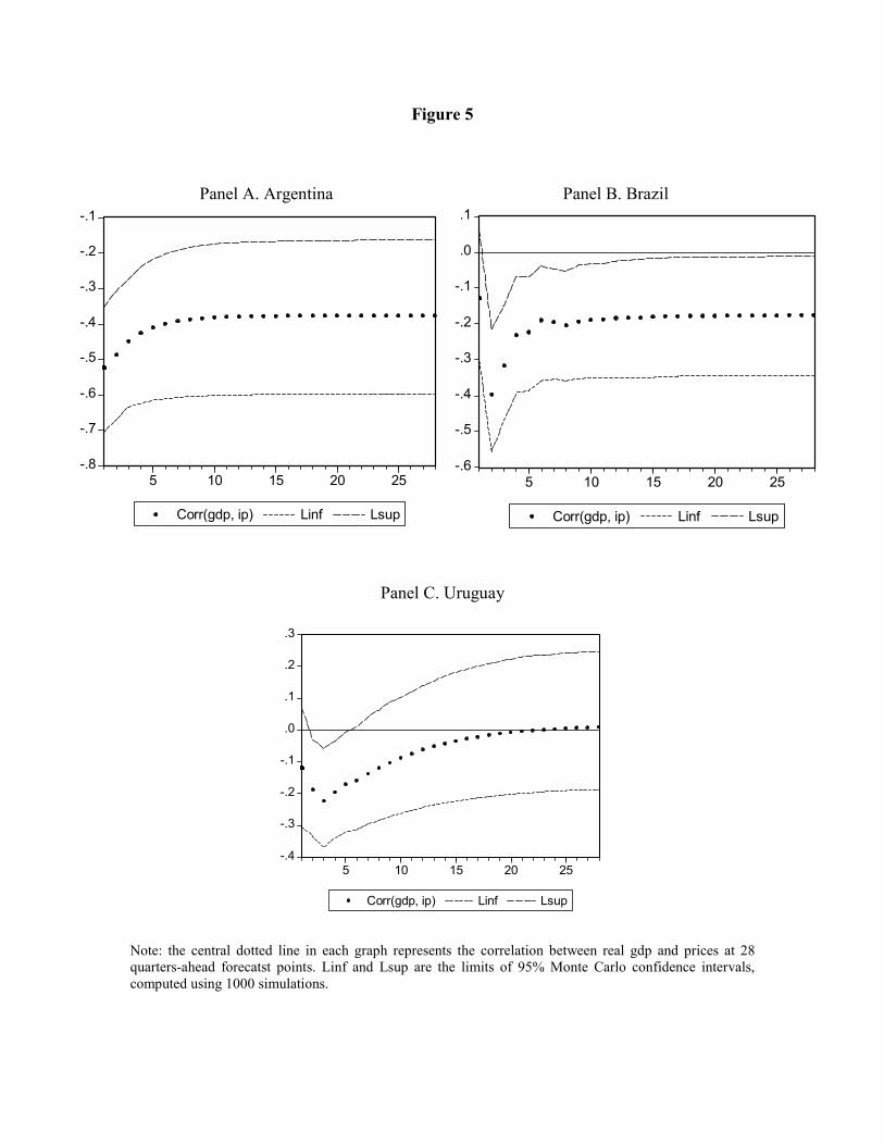
Figure 5

Panel A. Argentina Panel B. Brazil

Panel C. Uruguay

Note: the central dotted line in each graph represents the correlation between real gdp and prices at 28

quarters-ahead forecatst points. Linf and Lsup are the limits of 95% Monte Carlo confidence intervals,

computed using 1000 simulations.

-.8

-.7

-.6

-.5

-.4

-.3

-.2

-.1

5 10 15 20 25

Corr(gdp, ip) Linf Lsup

-.6

-.5

-.4

-.3

-.2

-.1

.0

.1

5 10 15 20 25


-.4

-.3

-.2

-.1

.0

.1

.2

.3

5 10 15 20 25


Figure 6. Panel A. Argentina

-.03

-.02

-.01

.00

.01

.02

.03

.04

.05

2 4 6 8 10 12 14 16 18 20-.03

-.02

-.01

.00

.01

.02

.03

.04

.05

2 4 6 8 10 12 14 16 18 20

-.12

-.08

-.04

.00

.04

.08

.12

.16

.20

.24

2 4 6 8 10 12 14 16 18 20-.12

-.08

-.04

.00

.04

.08

.12

.16

.20

.24

2 4 6 8 10 12 14 16 18 20

Accumulated Response to Cholesky One S.D. Innovations ± 2 S.E.

Accumulated Response of GDP to shock in GDP Accumulated Response of GDP to shock in RER

Accumulated Response of RER to shock in GDP Accumulated Response of RER to shock in RER

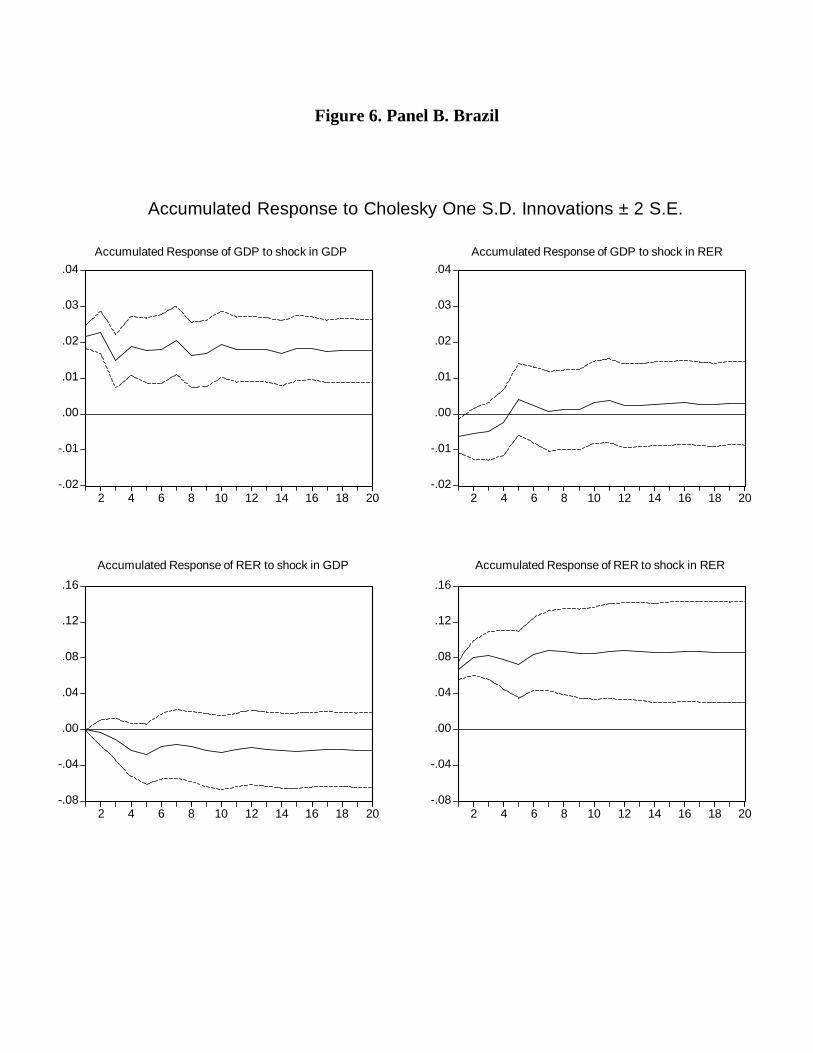
Figure 6. Panel B. Brazil

-.02

-.01

.00

.01

.02

.03

.04

2 4 6 8 10 12 14 16 18 20-.02

-.01

.00

.01

.02

.03

.04

2 4 6 8 10 12 14 16 18 20

-.08

-.04

.00

.04

.08

.12

.16

2 4 6 8 10 12 14 16 18 20-.08

-.04

.00

.04

.08

.12

.16

2 4 6 8 10 12 14 16 18 20




Figure 6. Panel C. Uruguay

-.02

.00

.02

.04

.06

.08

2 4 6 8 10 12 14 16 18 20-.02

.00

.02

.04

.06

.08

2 4 6 8 10 12 14 16 18 20

-.20

-.15

-.10

-.05

.00

.05

.10

2 4 6 8 10 12 14 16 18 20-.20

-.15

-.10

-.05

.00

.05

.10

2 4 6 8 10 12 14 16 18 20




Figure 7

Mercosur Business Cycle

-0.08

-0.06

-0.04

-0.02

0

0.02

0.04

0.06

I-88

III-8

8

I-89

III-8

9

I-90

III-9

0

I-91

III-9

1

I-92

III-9

2

I-93

III-9

3

I-94

III-9

4

I-95

III-9

5

I-96

III-9

6

I-97

III-9

7

I-98

III-9

8

I-99

III-9

9

I-00

III-0

0

I-01

III-0

1

I-02

III-0

2

I-03

% D

evia

tions

from

Com

mon

Tre

nd

Common Cycle

Figure 8

Argentina Brazil

-0.2

-0.15

-0.1

-0.05

0

0.05

0.1

0.15

0.2

I-88

I-89

I-90

I-91

I-92

I-93

I-94

I-95

I-96

I-97

I-98

I-99

I-00

I-01

I-02

I-03

Regional Cycle

-0.2

-0.15

-0.1

-0.05

0

0.05

0.1

0.15

0.2

I-88

I-89

I-90

I-91

I-92

I-93

I-94

I-95

I-96

I-97

I-98

I-99

I-00

I-01

I-02

I-03

% D

evia

tions

from

Com

mon

Tre

nd

Regional Cycle

% D

evia

tions

from

Com

mon

Tre

nd

Uruguay

-0.2

-0.15

-0.1

-0.05

0

0.05

0.1

0.15

0.2

I-88

I-89

I-90

I-91

I-92

I-93

I-94

I-95

I-96

I-97

I-98

I-99

I-00

I-01

I-02

I-03

% D

evia

tions

from

Com

mon

Tre

nd

Regional Cycle

Figure 9

Mercosur Common Cycle and Lagged Combined Country Risk

-10

-5

0

5

10

15

20

25

30

35

40

II-88

IV-8

8II-

89IV

-89

II-90

IV-9

0II-

91IV

-91

II-92

IV-9

2II-

93IV

-93

II-94

IV-9

4II-

95IV

-95

II-96

IV-9

6II-

97IV

-97

II-98

IV-9

8II-

99IV

-99

II-00

IV-0

0II-

01IV

-01

II-02

IV-0

2

Common Cycle Mercosur Combined Country Risks

References

Bayoumi, T. and Eichengreen, B. (1992), “Shocking aspects of european monetary unification,”

NBER, Working Paper 3949, Cambridge, January.

Bayoumi, T. and Mauro, P. (2001), “The Suitability of ASEAN for a Regional Currency

Arrangement,” World Economy, Vol. 24, Issue 7, pp. 933-954, July.

Basu, Susanto and Taylor, Alan M. (1999), “Business Cycle in International Historical Per-

spective,” Journal of Economic Perspectives, Vol. 13, N 2, pp. 45-68, Spring.

Baxter, M. and King, R. G. (1995), “Measuring business cycles approximate Band-Pass filters

for economic time series,” NBER, Working Paper 5022, February.

Bebczuk, R. N.; Fanelli, J. M. and Pradelli, J.J. (2002), “Determinants and Concequences of

Financial Constraints Facing Firms in Argentina,” Research Network Working Papers,

R-453, Research Department, IADB-CEDES, July.

Blanchard, O. and Quah, D. (1989), “The Dynamic Effects of Aggregate Demand and Supply

Disturbances,” American Economic Review, Vol. 79, pp. 655-673, September.

Calvo, G. and Reinhart, C. (1999), “When Capital Inflows Come to a Sudden Stop: Conse-

quences and Policy Options,” Preliminary Draft, June.

(http://www.bsos.umd.edu/econ/ciecpp.htm)

Calvo, G. and Reinhart, C. (2002), “Fear of Floating,” Quarterly Journal of Economics, Vol.

117, Issue 2, pp. 379-408, May.

Cheung, Yin-Wong and Westerman, Frank (2000), “Does Austria to the German or the US

Business Cycle?,” International Journal of Finance and Economics, Vol. 5. Issue 1, pp.

33-42, February.

Dempster A.P., N.M. Laird and D.B. Rubin (1977), “Maximum likelihood from incomplete

data,” Journal of the Royal Statistical Society Ser. B 39:1-38.

Den Haan, W. J. (2000), “The comovement between output and prices,” Journal of Monetary

Economics, N 46, pp. 3-30.

42

Den Haan, W. J. and Sumner, Steven (2001), “The comovements between real activity and

prices in the G7,” NBER, Working Paper 8195, March.

Eichengreen, B. (1998), “Does Mercosur need a single currency?,” NBER, Working Paper

6821, Cambridge, December.

Eichengreen, B. and Taylor, A. M. (2003), “The monetary consequences of a free trade area

of the Americas,” NBER, Working Paper 9666, Cambridge, April.

Fanelli, J. M. (2001), “Coordinacion macroeconomica en el Mercosur: Marco analıtico y hechos

estilizados,” in Coordinacion de polıticas macroeconomicas en el MERCOSUR, Red de

Investigaciones Economicas del MERCOSUR, Siglo XXI de Argentina Editores, Ch. 1,

pp. 1-23, April.

Fanelli, J. M.; Gonzalez-Rozada, M. and Keifman, Saul (2001), “Comercio, regimen cambiario

y volatilidad. Una vision desde la Argentina de la coordinacion macroeconomica en

el Mercosur,” in Coordinacion de polıticas macroeconomicas en el MERCOSUR, Red de

Investigaciones Economicas del MERCOSUR, Siglo XXI de Argentina Editores, Ch. 2,

pp. 25-70, April.

Fanelli, J. M. and Heymann, D. (2002), “Dilemas monetarios en la Argentina,” Revista de

Desarrollo Economico, No. 165, Vol. 42, Abril-Junio.

Kenen, Peter B. (1969), “The Theory of optimum Currency Areas: An Eclectic View,”

in Robert A. Mundell and Alexander K. Swoboda (eds). Monetary Problems of the

International Economy (Chicago: University of Chicago Press).

Kouparitsas, Michael A. (2002), “Understanding U.S. regional cyclical comovement: How

important are spillovers and common shocks?,” Economic Perspectives, Fourth Quarter,

Federal Reserve Bank of Chicago, Chicago, US.

Machinea, Jose Luis (2002), “Exchange Rate Instability in Mercosur: Causes, Problems and

Possible Solutions,” unpublished manuscript, Inter-American Development Bank, July.

Rogoff, K. (1996), “The Purchasing Power Parity Puzzle,” in Journal of Economic Literature,

The American Economic Association, USA, Vol. XXXIV, N 2, pp. 647-668, June.

43

Watson, M. W. and Engle, R. F. (1983), “Alternative algorithms for the estimation of dynamic

factor, MIMIC, and varying coefficients models,” Journal of Econometrics, Vol. 23, pp.

385-400.

Watson, M. W. (1986), “Univariate detrending methods with stochastic trends,” Journal of

Monetary Economics, Vol. 18, pp. 49-75.

44

Appendix 1

Table A.1: Estimation of Argentina’s VAR(2) Model

Vector Autoregression Estimates

Sample: 1980:1 2003:1

Dependent Variables

Independent Variables ∆ ln (gdp)t ∆ ln (ip)t

∆ ln (gdp)t−1 0.2123 −1.3449

t-Statistic 1.70 −1.23

∆ ln (gdp)t−2 0.0157 2.2920

t-Statistic 0.13 2.23

∆ ln (ip)t−1 0.0120 0.3870


∆ ln (ip)t−2 −0.0044 0.3601

t-Statistic −0.33 3.09

C −0.0004 0.0495


R-squared 0.0367 0.4363

F -Statistic 0.8089 16.4442

45

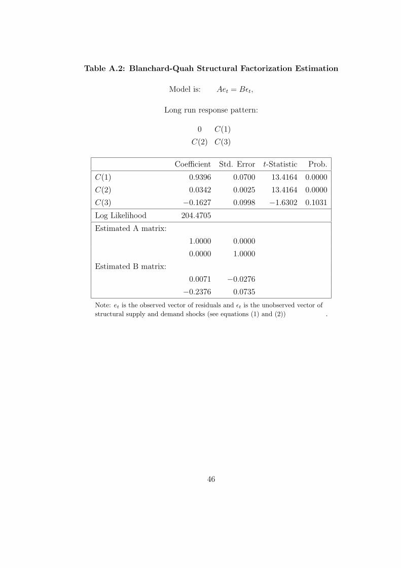
Table A.2: Blanchard-Quah Structural Factorization Estimation

Model is: Aet = Bεt,

Long run response pattern:

0 C(1)

C(2) C(3)


C(1) 0.9396 0.0700 13.4164 0.0000

C(2) 0.0342 0.0025 13.4164 0.0000

C(3) −0.1627 0.0998 −1.6302 0.1031

Log Likelihood 204.4705

Estimated A matrix:

1.0000 0.0000

0.0000 1.0000

Estimated B matrix:

0.0071 −0.0276

−0.2376 0.0735

Note: et is the observed vector of residuals and εt is the unobserved vector ofstructural supply and demand shocks (see equations (1) and (2)) .

46

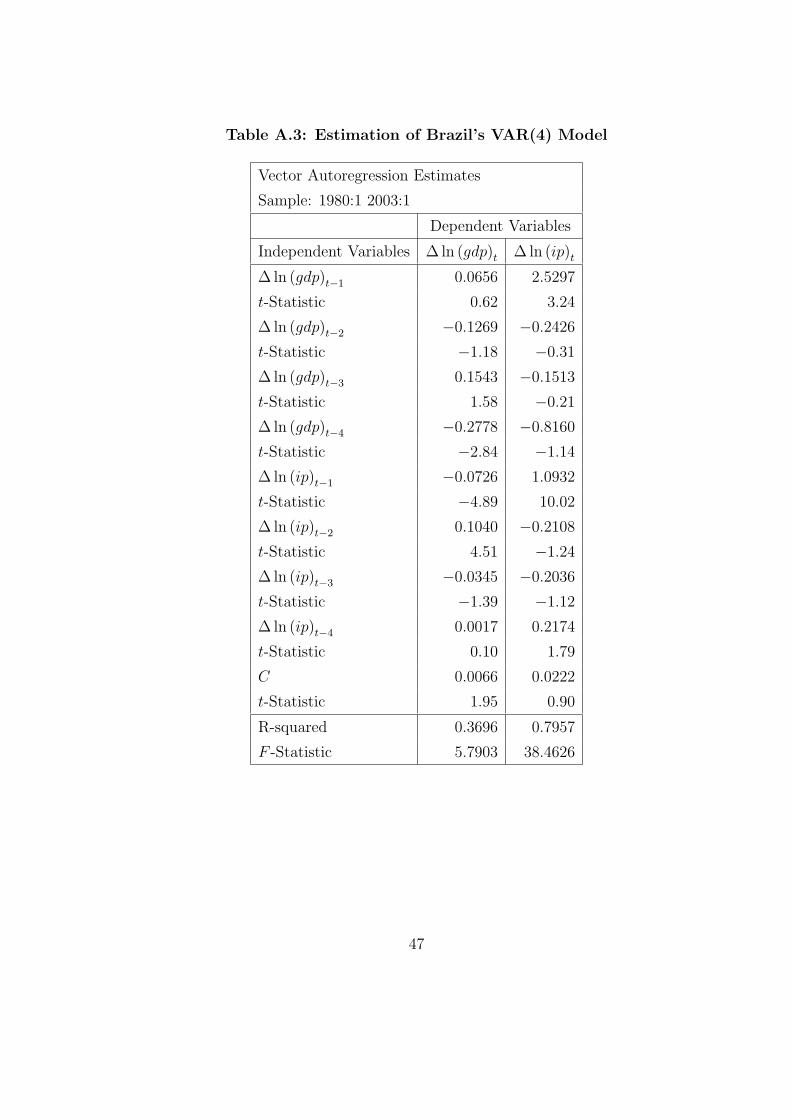
Table A.3: Estimation of Brazil’s VAR(4) Model


Sample: 1980:1 2003:1

Dependent Variables


∆ ln (gdp)t−1 0.0656 2.5297


∆ ln (gdp)t−2 −0.1269 −0.2426

t-Statistic −1.18 −0.31

∆ ln (gdp)t−3 0.1543 −0.1513


∆ ln (gdp)t−4 −0.2778 −0.8160


∆ ln (ip)t−1 −0.0726 1.0932


∆ ln (ip)t−2 0.1040 −0.2108


∆ ln (ip)t−3 −0.0345 −0.2036


∆ ln (ip)t−4 0.0017 0.2174


C 0.0066 0.0222


R-squared 0.3696 0.7957

F -Statistic 5.7903 38.4626

47




0 C(1)

C(2) C(3)


C(1) 1.4024 0.1057 13.2665 0.0000

C(2) 0.0172 0.0013 13.2665 0.0000

C(3) −0.0927 0.1496 −0.6195 0.5356


Estimated A matrix:

1.0000 0.0000

0.0000 1.0000

Estimated B matrix:

0.0018 −0.0202

0.1457 0.0323


48

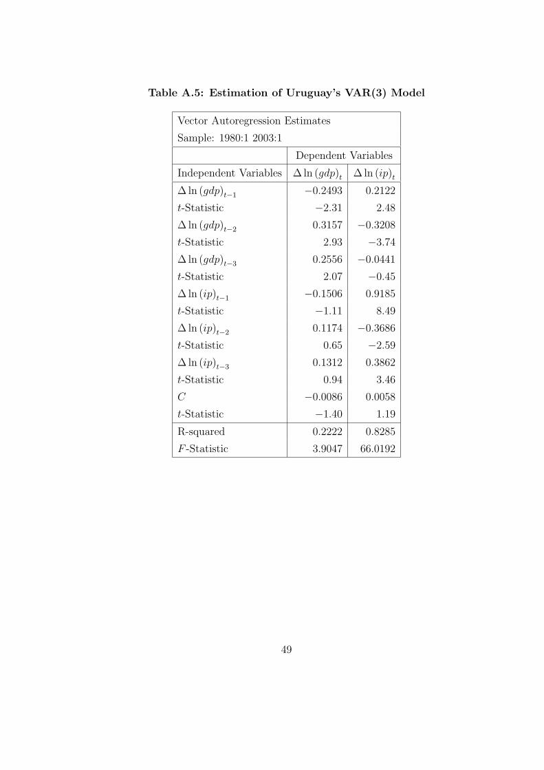
Table A.5: Estimation of Uruguay’s VAR(3) Model


Sample: 1980:1 2003:1

Dependent Variables


∆ ln (gdp)t−1 −0.2493 0.2122


∆ ln (gdp)t−2 0.3157 −0.3208


∆ ln (gdp)t−3 0.2556 −0.0441


∆ ln (ip)t−1 −0.1506 0.9185


∆ ln (ip)t−2 0.1174 −0.3686


∆ ln (ip)t−3 0.1312 0.3862


C −0.0086 0.0058


R-squared 0.2222 0.8285

F -Statistic 3.9047 66.0192

49




0 C(1)

C(2) C(3)


C(1) 0.2323 0.0174 13.3416 0.0000

C(2) 0.0453 0.0034 13.3416 0.0000

C(3) 0.1495 0.0271 5.5246 0.0000


Estimated A matrix:

1.0000 0.0000

0.0000 1.0000

Estimated B matrix:

0.0227 0.0161

−0.0148 0.0165


50

Table A.7: Estimation of Argentina’s VAR(2) Model


Sample: 1980:1 2003:1

Dependent Variables

Independent Variables ∆ ln (gdp)t ∆ ln (rer)t

∆ ln (gdp)t−1 0.1447 −0.1719


∆ ln (gdp)t−2 0.0340 −1.6710


∆ ln (rer)t−1 −0.0370 −0.1548


∆ ln (rer)t−2 0.0130 −0.1890


C 0.0016 0.0197


R-squared 0.1069 0.0953

F -Statistic 2.5424 2.2372

51

Table A.8: Estimation of Brazil’s VAR(5) Model


Sample: 1980:1 2003:1

Dependent Variables


∆ ln (gdp)t−1 0.0634 −0.1584


∆ ln (gdp)t−2 −0.3751 −0.3094


∆ ln (gdp)t−3 0.2410 −0.5313


∆ ln (gdp)t−4 −0.2169 −0.1954


∆ ln (gdp)t−5 0.2161 0.2567


∆ ln (rer)t−1 0.0163 0.1846


∆ ln (rer)t−2 −0.0289 −0.0195


∆ ln (rer)t−3 0.0677 −0.1246


∆ ln (rer)t−4 0.0632 −0.0425


∆ ln (rer)t−5 −0.0110 0.2638


C 0.0059 0.0081


R-squared 0.2529 0.1282

F -Statistic 2.5729 1.1176

52

Table A.3: Estimation of Uruguay’s VAR(4) Model


Sample: 1980:1 2003:1

Dependent Variables


∆ ln (gdp)t−1 −0.1850 −0.1118


∆ ln (gdp)t−2 0.3633 −0.7498


∆ ln (gdp)t−3 0.3153 −0.3998


∆ ln (gdp)t−4 −0.0850 −0.6684


∆ ln (rer)t−1 0.0282 0.3189


∆ ln (rer)t−2 −0.0862 −0.4033


∆ ln (rer)t−3 0.0688 0.0910


∆ ln (rer)t−4 0.0391 0.0260


C −0.0003 0.0116


R-squared 0.2194 0.3999

F -Statistic 2.7765 6.5806

53

Business Cycles and Macroeconomic Policy Coordination in ...

Documents

Transcript of Business Cycles and Macroeconomic Policy Coordination in ...