BURST CORRECTION CODING FROM LOW-DENSITY … · BURST CORRECTION CODING FROM LOW-DENSITY...

BURST CORRECTION CODING FROM LOW-DENSITY PARITY-CHECK CODES

by

Wai Han FongA Dissertation

Submitted to theGraduate Faculty

ofGeorge Mason UniversityIn Partial fulfillment of

The Requirements for the Degreeof

Doctor of PhilosophyElectrical and Computer Engineering

Committee:

Dr. Shih-Chun Chang, Dissertation Director

Dr. Shu Lin, Dissertation Co-Director

Dr. Geir Agnarsson, Committee Member

Dr. Bernd-Peter Paris, Committee Member

Dr. Brian Mark, Committee Member

Dr. Monson Hayes, Department Chair

Dr. Kenneth S. Ball, Dean, The VolgenauSchool of Engineering

Date: Fall Semester 2015George Mason UniversityFairfax, VA

Burst Correction Coding from Low-Density Parity-Check Codes

A dissertation submitted in partial fulfillment of the requirements for the degree ofDoctor of Philosophy at George Mason University

By

Wai Han FongMaster of Science

George Washington University, 1992Bachelor of Science

George Washington University, 1984

Director: Dr. Shih-Chun Chang, Associate ProfessorDepartment of Electrical and Computer Engineering

George Mason UniversityFairfax, VA

Co-Director: Dr. Shu Lin, ProfessorDepartment of Electrical and Computer Engineering

University of CaliforniaDavis, CA

Fall Semester 2015George Mason University

Fairfax, Virginia

Copyright c© 2015 by Wai Han FongAll Rights Reserved

ii

Dedication

I dedicate this dissertation to my beloved parents, Pung Han and Soo Chun; my wife, Ellen;children, Corey and Devon; and my sisters, Rose and Agnes.

iii

Acknowledgments

I would like to express my sincere gratitude to my two Co-Directors: Shih-Chun Chang andShu Lin without whom this would not be possible. In addition, I would especially like tothank Shu Lin for his encouragement, his creativity and his generosity, all of which are aninspiration to me. A special thanks to my entire family who provided much moral support,particularly my cousin, Manfai Fong. I would also like to thank the following people fortheir support and encouragement: Pen-Shu Yeh, Victor Sank, Shannon Rodriguez, WingLee, Mae Huang, Brian Gosselin, David Fisher, Pamela Barrett, Jeff Jaso, and ManuelVega. And thanks to Qin Huang who collaborated in Section 6.3 and provided simulationresults for Section 6.4. And special thanks to my many influential teachers at GMU. Finally,at my high school, much gratitude goes to my math teacher Charles Baumgartner.

iv

Table of Contents

Page

List of Figures . . . . . . . . . . . . . . . . . . . . . . . . . . . . . . . . . . . . . . . . viii

Abstract . . . . . . . . . . . . . . . . . . . . . . . . . . . . . . . . . . . . . . . . . . . xi

1 Introduction . . . . . . . . . . . . . . . . . . . . . . . . . . . . . . . . . . . . . . 1

1.1 Background . . . . . . . . . . . . . . . . . . . . . . . . . . . . . . . . . . . . 1

1.2 Motivation . . . . . . . . . . . . . . . . . . . . . . . . . . . . . . . . . . . . 2

1.3 Summary of Research . . . . . . . . . . . . . . . . . . . . . . . . . . . . . . 3

2 Communication Systems Background . . . . . . . . . . . . . . . . . . . . . . . . 6

2.1 Channel Characteristics . . . . . . . . . . . . . . . . . . . . . . . . . . . . . 8

2.1.1 Random Error/Erasure . . . . . . . . . . . . . . . . . . . . . . . . . 8

2.1.2 Burst Error/Erasure . . . . . . . . . . . . . . . . . . . . . . . . . . . 11

2.2 Linear Block Codes for Error/Erasure Correction . . . . . . . . . . . . . . . 12

2.2.1 Cyclic Codes . . . . . . . . . . . . . . . . . . . . . . . . . . . . . . . 13

2.2.2 Quasi-Cyclic Codes . . . . . . . . . . . . . . . . . . . . . . . . . . . . 14

3 Low-Density Parity-Check Codes . . . . . . . . . . . . . . . . . . . . . . . . . . . 15

3.1 Introduction . . . . . . . . . . . . . . . . . . . . . . . . . . . . . . . . . . . . 15

3.2 Technical Description . . . . . . . . . . . . . . . . . . . . . . . . . . . . . . 17

3.3 LDPC Code Construction . . . . . . . . . . . . . . . . . . . . . . . . . . . . 21

3.3.1 Mackay Codes . . . . . . . . . . . . . . . . . . . . . . . . . . . . . . 22

3.4 Structured LDPC Codes . . . . . . . . . . . . . . . . . . . . . . . . . . . . . 22

3.4.1 Euclidean Geometry Codes . . . . . . . . . . . . . . . . . . . . . . . 22

3.4.2 Product Codes . . . . . . . . . . . . . . . . . . . . . . . . . . . . . . 24

3.5 Sum Product Algorithm . . . . . . . . . . . . . . . . . . . . . . . . . . . . . 26

3.6 Min-Sum Decoder . . . . . . . . . . . . . . . . . . . . . . . . . . . . . . . . 28

3.7 Erasure Correcting Algorithm . . . . . . . . . . . . . . . . . . . . . . . . . . 29

4 Burst Erasure Correction Ensemble Analysis for Random LDPC Codes . . . . . 30

4.1 Introduction . . . . . . . . . . . . . . . . . . . . . . . . . . . . . . . . . . . . 30

4.2 Zero-Span Characterization for Random LDPC Codes . . . . . . . . . . . . 33

4.2.1 Background . . . . . . . . . . . . . . . . . . . . . . . . . . . . . . . . 33

v

4.2.2 Recursive Erasure Decoding . . . . . . . . . . . . . . . . . . . . . . . 33

4.2.3 Zero-Span Definition . . . . . . . . . . . . . . . . . . . . . . . . . . . 34

4.3 Statistical Analysis for the General Ensemble of Random LDPC Codes . . . 39

4.3.1 Moments of the Zero-Covering Span PMF . . . . . . . . . . . . . . . 44

4.3.2 Asymptotic Burst Erasure Correction Performance . . . . . . . . . . 51

4.3.3 Probability Mass Function of the Correctible Profile γ . . . . . . . . 52

4.4 Truncated General Ensemble Analysis . . . . . . . . . . . . . . . . . . . . . 57

4.4.1 The Truncated Correctible Profile γ . . . . . . . . . . . . . . . . . . 62

4.4.2 Regions of Analysis . . . . . . . . . . . . . . . . . . . . . . . . . . . 66

5 Expurgated Ensemble of Random LDPC Codes for Burst Erasures . . . . . . . . 75

5.1 Statistical Analysis . . . . . . . . . . . . . . . . . . . . . . . . . . . . . . . . 75

5.1.1 Effective Arrival Rate . . . . . . . . . . . . . . . . . . . . . . . . . . 75

5.1.2 Updated Equations . . . . . . . . . . . . . . . . . . . . . . . . . . . . 80

5.2 Data Results . . . . . . . . . . . . . . . . . . . . . . . . . . . . . . . . . . . 81

6 Multiple Burst Error Correction Coding . . . . . . . . . . . . . . . . . . . . . . . 91

6.1 LDPC Codes Expanded . . . . . . . . . . . . . . . . . . . . . . . . . . . . . 91

6.1.1 OSMLD Algorithm . . . . . . . . . . . . . . . . . . . . . . . . . . . . 92

6.1.2 Superposition Construction of LDPC Codes . . . . . . . . . . . . . . 94

6.2 Multiple Phased-Burst Correcting LDPC Codes Based on CPM Constituent

Codes . . . . . . . . . . . . . . . . . . . . . . . . . . . . . . . . . . . . . . . 95

6.3 Binary MPBC Codes . . . . . . . . . . . . . . . . . . . . . . . . . . . . . . . 96

6.4 Performances over the AWGN Channels and the BEC . . . . . . . . . . . . 99

6.5 Multiple Phased-Burst Error Correction Bound . . . . . . . . . . . . . . . . 103

6.6 Single Burst Correction Bound . . . . . . . . . . . . . . . . . . . . . . . . . 117

7 Multiple Burst Erasures Correction Coding . . . . . . . . . . . . . . . . . . . . . 120

7.1 Product Codes for Erasure Correction . . . . . . . . . . . . . . . . . . . . . 120

7.1.1 Parity-Check Matrix Structure . . . . . . . . . . . . . . . . . . . . . 124

7.2 Analysis of LDPC Product Codes . . . . . . . . . . . . . . . . . . . . . . . . 126

7.2.1 Multiple Burst Erasure Correcting Capability . . . . . . . . . . . . . 128

7.3 Decoding Algorithms . . . . . . . . . . . . . . . . . . . . . . . . . . . . . . . 131

7.4 Product Code Multiple Burst Erasure Decoding Algorithm . . . . . . . . . 131

7.4.1 Examples of LDPC Product Codes for Burst Erasure Correction . . 132

7.5 Product Code LDPC Decoding Algorithm for AWGN . . . . . . . . . . . . 135

7.5.1 Two-Stage LDPC Product Code Decoder . . . . . . . . . . . . . . . 135

7.6 Product LDPC Code Examples and Results . . . . . . . . . . . . . . . . . . 137

vi

8 Conclusion . . . . . . . . . . . . . . . . . . . . . . . . . . . . . . . . . . . . . . . 143

Bibliography . . . . . . . . . . . . . . . . . . . . . . . . . . . . . . . . . . . . . . . . . 145

vii

List of Figures

Figure Page

2.1 Communications Channel . . . . . . . . . . . . . . . . . . . . . . . . . . . . 7

2.2 Simplified Communications Channel . . . . . . . . . . . . . . . . . . . . . . 7

2.3 Binary Input Additive White Gaussian Noise Channel . . . . . . . . . . . . 9

2.4 Binary Erasure Channel . . . . . . . . . . . . . . . . . . . . . . . . . . . . . 10

2.5 Binary Symmetric Channel . . . . . . . . . . . . . . . . . . . . . . . . . . . 10

3.1 Tanner Graph Example . . . . . . . . . . . . . . . . . . . . . . . . . . . . . 18

4.1 (240,160) Randomly Generated LDPC Code Forward Zero-Covering Span

Profile and Forward Correctible Profile . . . . . . . . . . . . . . . . . . . . . 39

4.2 (240,160) Randomly Generated LDPC Code Backward Zero-Covering Span

Analysis and Backward Correctible Profile . . . . . . . . . . . . . . . . . . . 40

4.3 (240,160) LDPC Code Scatter Plot . . . . . . . . . . . . . . . . . . . . . . . 40

4.4 (240,160) LDPC δF Histogram . . . . . . . . . . . . . . . . . . . . . . . . . 41

4.5 EG (255,175) LDPC Code Forward Span Analysis . . . . . . . . . . . . . . 41

4.6 EG (255,175) LDPC Code Backward Span Analysis . . . . . . . . . . . . . 42

4.7 EG (255,175) LDPC Code Scatter Plot . . . . . . . . . . . . . . . . . . . . . 42

4.8 Forward Zero-Covering Span Ensemble PMF for Randomly Generated 80×2000 LDPC Matrices of Constant Column Weight . . . . . . . . . . . . . . . 45

4.9 Mean and Standard Deviation of Zero-Spans for Various Block Sizes . . . . 50

4.10 Asymptotic Mean of Zero-Covering Spans . . . . . . . . . . . . . . . . . . . 51

4.11 Example LDPC code N = 100, 000 . . . . . . . . . . . . . . . . . . . . . . . 56

4.12 Zero-Covering Span Mean . . . . . . . . . . . . . . . . . . . . . . . . . . . . 61

4.13 Standard Deviation of Zero-Covering Spans . . . . . . . . . . . . . . . . . . 61

4.14 Mean of Correctible profile PMF of Zero-Spans for N=100 . . . . . . . . . . 63

4.15 Mean of Correctible profile PMF of Zero-Spans for N=1,000 . . . . . . . . . 64

4.16 Mean of Correctible profile PMF of Zero-Spans for N=10,000 . . . . . . . . 65

4.17 Example LDPC code for N = 100 . . . . . . . . . . . . . . . . . . . . . . . . 66

4.18 α Factor . . . . . . . . . . . . . . . . . . . . . . . . . . . . . . . . . . . . . . 68

viii

4.19 A Comparison of Analytical Thresholds . . . . . . . . . . . . . . . . . . . . 73

5.1 The Effective Arrival Rate . . . . . . . . . . . . . . . . . . . . . . . . . . . . 78

5.2 Row Weight Distribution Analysis . . . . . . . . . . . . . . . . . . . . . . . 79

5.3 Example LDPC code for N = 1, 000 . . . . . . . . . . . . . . . . . . . . . . 82

5.4 Zero-covering span profile PMF of LDPC Matrices N=100 . . . . . . . . . . 82

5.5 Gamma PMF with Block Size N=100 . . . . . . . . . . . . . . . . . . . . . 83

5.6 Zero-covering span profile PMF of LDPC Matrices N=1,000 . . . . . . . . . 84

5.7 Gamma PMF with Block Size N=1,000 . . . . . . . . . . . . . . . . . . . . 84

5.8 Zero-covering span profile PMF of LDPC Matrices N=10,000 . . . . . . . . 85

5.9 Gamma PMF with Block Size N=10,000 . . . . . . . . . . . . . . . . . . . . 85

5.10 Correctible profile PMF of Zero-Spans for Expurgated Ensemble N=100 . . 87

5.11 Correctible profile PMF of Zero-Spans for Expurgated Ensemble N=1000 . 88

5.12 Correctible profile PMF of Zero-Spans for Expurgated Ensemble N=10,000 88

6.1 Simulation Results of binary QC (4340, 3485) LDPC Code over the AWGN

Channels . . . . . . . . . . . . . . . . . . . . . . . . . . . . . . . . . . . . . 101

6.2 Convergence of binary QC (4340, 3485) LDPC Code over AWGN Channels 101

6.3 Simulation Results of binary QC (4340, 3485) LDPC Code over the BEC

Channel . . . . . . . . . . . . . . . . . . . . . . . . . . . . . . . . . . . . . . 102

6.4 Simulation Results of binary QC (37800,34035) LDPC Code over the AWGN

Channels . . . . . . . . . . . . . . . . . . . . . . . . . . . . . . . . . . . . . 102

6.5 MPBC Bound with a gap restriction for a Codelength of 10 Subblocks and

100 bits per Subblock . . . . . . . . . . . . . . . . . . . . . . . . . . . . . . 112

6.6 MPBC without a gap restriction for a Codelength of 10 Subblocks and 100

bits per Subblock . . . . . . . . . . . . . . . . . . . . . . . . . . . . . . . . . 114

6.7 MPBC Bounds with and without a gap restriction . . . . . . . . . . . . . . 115

7.1 Product Code Array . . . . . . . . . . . . . . . . . . . . . . . . . . . . . . . 122

7.2 BEC Performance of EG(63,37)×EG(63,37) . . . . . . . . . . . . . . . . . . 133

7.3 BEC Performance of SPC(63,62)×EG(255,175) . . . . . . . . . . . . . . . . 134

7.4 Two-Stage LDPC Product Code Decoder . . . . . . . . . . . . . . . . . . . 136

7.5 EG (255,175) LDPC Code with SPA in AWGN Channel . . . . . . . . . . . 138

7.6 PEG (255,175) Code with SPA in AWGN Channel . . . . . . . . . . . . . . 138

7.7 PEG (255,175)×PEG (255,175) in AWGN Channel . . . . . . . . . . . . . . 139

7.8 EG (255,175)×EG (255,175) in AWGN Channel . . . . . . . . . . . . . . . 140

7.9 PEG (255,175)×SPC (64,63) in AWGN Channel . . . . . . . . . . . . . . . 141

ix

7.10 EG (255,175)×SPC (64,63) in AWGN Channel . . . . . . . . . . . . . . . . 141

x

Abstract

BURST CORRECTION CODING FROM LOW-DENSITY PARITY-CHECK CODES

Wai Han Fong, PhD

George Mason University, 2015

Dissertation Director: Dr. Shih-Chun Chang

Dissertation Co-Director: Dr. Shu Lin

This thesis explores techniques and theoretical bounds on efficiently encodable low-density

parity-check (LDPC) codes for correcting single and multiple bursts of erasures and/or er-

rors. The approach is to construct good burst correction codes via superposition techniques

from smaller constituent codes, such as product codes and/or use existing codes with newer

decodings, such as randomly generated LDPC codes with simple recursive erasure decod-

ing. Another goal is to design codes that perform well in a random error environment as

well a bursty environment for some channels that change from one state to the other, i.e. a

satellite optical link that suffers from fades due to atmospheric scintillation. Novel decoding

approaches are explored, i.e. iterative decoding of constituent codes and/or decoding over

the entire code. The motivation for this work is the use of multiple burst correction coding

for the following types of applications: 1) optical laser communications where atmospheric

turbulence create burst errors; 2) wireless communications where fading is created by mul-

tipath, or interference from random impulses and jamming; and 3) packet networks where

traffic congestion can create erasure bursts from packet losses.

Chapter 1: Introduction

This thesis is focused on finding new solutions to the classical problem of burst erasure

and burst error control for bursty channels. Bursty channels are the result of correlated

errors/erasures patterns. Traditional solutions to the this problem involve implementing

Reed-Solomon codes. Specifically, this work is focused on exploiting low-density parity-

check (LDPC) codes to solve this problem. Recently, there have been work in this field,

[1–3]. We will explore and extend LDPC codes; and apply these codes to multi-dimensional

structures, such as product codes and others, as well as use randomly generated LDPC

codes in novel approaches.

1.1 Background

Many channels experience bursty distortions that will corrupt a sequence of transmission

symbols. For instance, thermal eddies create atmospheric turbulence called scintillation that

a laser beam transmitted through free-space must contend with. As a result of the diffraction

and refraction of the light through these eddies, the intensity of the beam will typically

experience 10 millisecond fades every second at the receiver on an orbiting spacecraft [4].

Some optical links use a very large LDPC code for random error correction, concatenated

with a one to two second interleaver to mitigate this distortion [5]. The interleaver will

redistribute the burst errors/erasures to different codewords in an effort to produce a more

random error distribution at each codeword. This places less of a burden on a single or a

sequence of LDPC codewords to correct the entire burst. The complexity requirement is

quite large however, given that the LDPC code used is on the order of 64,000 bit blocks that

sometimes will be concatenated with another code to remove the residual error floors. This

1

requirement can slow down the data rate to values that are much less than the potential

raw optical transmission rate or require a lot of parallelism to maintain data rate.

Another channel that is noteworthy is the packet network. Lost packets or packets received

with errors create a large gap in the transmission of files. Packetized data typically will

have an error control field that can be used detect the presence of errors in the received

packet. Typically, the detection mechanism is a cyclic redundancy check (CRC) field. Since,

the location of the erred packet, in a large sequence of packets, is known, these packets are

defined as erased packets and the symbols within these packets are erased symbols. Usually,

the network will ask for retransmission of these erased packets [6] thus consuming channel

bandwidth.

Finally, the wireless channel must deal with, in general, two types of fades: 1) large-scale

fading caused by path loss and/or shadowing from large obstructions; and 2) small-scale

fading caused by multi-path or reflections along the transmission path creating constructive

and destructive interference at the receiver. Depending on the time scale, a number of

solutions can be considered to combat these fades, i.e. time diversity, frequency diversity,

antenna diversity, etc [7]. However, if error/erasure control codes can be implemented

efficiently, these techniques can certainly compete with current solutions.

Each of these channels experiences a similar phenomena, i.e. there is a noise process that

will affect multiple symbols over a certain time scale. Therefore we search for simple burst

correction algorithms that can: 1) impact the complexity for the free space laser communi-

cations; 2) save overall channel bandwidth in the case of packet networking: and 3) simplify

techniques that is currently used in wireless channels.

1.2 Motivation

The channel distortions mentioned above are strong motivating factors in this thesis. We

try to find novel low complexity solutions to these problems that are much different than

2

what is typically used today in bursty channels. We are motivated to use LDPC codes since

they have been shown to approach the capacity for random errors but have seen very few

application to bursty channels. For this reason alone, we will explore the possible use of

LDPC codes in this manner; and develop coding structures and decoding techniques that

are specifically designed to combat bursty errors/erasures unlike the LDPC code used in

the optical link above.

The typical and general error correction coding technique for burst correction is to use

Reed-Solomon Codes in conjunction with a very large interleaver. This can be seen in mass

storage mediums such as the Compact Discs (CD)[8], Blu-ray Discs, Digital Versatile Discs

(DVD) [9]; and satellite communication standards, [10, 11]. Since Reed-Solomon codes are

GF(q) non-binary codes for random errors, this approach may consume too much bandwidth

or require too much decoding and interleaver complexities to overcome the bursts. It would

be preferential to develop a singular burst correcting technique that can be tuned more

accurately for the particular channel statistics so that complexity and required bandwidth

can be reduced. That is, given an average burst length over an average period of time, a

simple coding technique can be designed to mitigate this distortion. This is the primary

motivation for this thesis.

We are also motivated to find the theoretical limits of burst correction. We wish to measure

how well our solutions compare with these limits. And we would to like to connect these

limits to already published bounds to ensure that the results are valid.

1.3 Summary of Research

The objectives are: 1) discover new techniques to correct a specified length of burst era-

sures/errors, 2) analyze the burst correction capability of these techniques, and 3) develop

theoretical limits for burst correction for these techniques. To this end, our main results

are described in Chapters 4 to 7.

3

In Chapters 4 and 5, a low complexity recursive erasure decoding (RED) algorithm utilizing

a recursive symbol-by-symbol correction scheme was applied to LDPC codes. In Chapter 4,

the analysis to characterize the burst erasure correction capability of an erasure correction

code using this scheme was based on the concept of zero-span. This is the length of a con-

secutive string of zeros between two unique non-zero entries within a row of the parity-check

matrix. This chapter presents statistical characterization of zero-spans for the ensemble of

randomly generated Low Density Parity-Check (LDPC) codes with parity-check matrices of

constant column weight for burst erasure correction. The average burst erasure correction

performance is analyzed for small to large block sizes. And the asymptotic performance,

as the block size approach infinity, is analyzed and it is shown that the correction perfor-

mance is asymptotically good. The statistical analysis is performed for the general ensemble

consisting of all random LDPC matrices of constant column weight.

In Chapter 5, the expurgated ensemble is analyzed, consisting of all random LDPC matrices

of constant column weight without rows that consist of all zeros or rows containing a single

non-zero. The reason for the second ensemble is that the RED algorithm cannot be used with

these rows. Therefore removing them from the general ensemble is a necessary procedure

unless the likelihood of these of rows is very small. We compare both ensembles in mean

burst erasure correction capability over various block lengths and column weights of LDPC

matrices.

In Chapters 6 and 7, the focus turns to multiple burst error/erasure correction. Two major

achievements are presented in Chapter 6. The first achievement is the construction of codes

for multiple phased-burst error correction (MPBC). A class of LDPC codes is presented

based on the superposition of circulant permutation matrices (CPM) as constituent ma-

trices. This technique can produce binary quasi-cyclic low-density parity-check (LDPC)

codes. These codes can effectively correct multiple phased-burst errors and erasures and

other hybrid types of error-patterns by simple one-step-majority-logic decoding (OSMLD).

Moreover, they perform very well over both binary erasure and additive white Gaussian

4

noise (AWGN) channels. The second achievement is the derivation of two MPBC bounds

for achievable code rate. The class of superposition codes based on CPM constituent ma-

trices is shown to be tight with respect to these bounds. One bound, when reduced to the

special case of a single burst for one codeword, is proved to be a generalized Abramson

bound for single burst-error (SBC) correction [12, p. 202].

In Chapter 7, a second class of multiple burst erasure correction is presented and is based

on product code construction. By using LDPC constituent codes, a novel multiple burst

erasure decoding algorithm is presented that will allow for the correction of a single large

erasure burst or smaller multiple erasure phased-bursts. Also, these codes are shown to

perform well in an AWGN channel using message passing algorithms.

5

Chapter 2: Communication Systems Background

The field of error control coding focuses on the study and mitigation of error phenomena

when transmitting information symbols over a statistically noisy channel. A diagram of

a communications link is shown in Figure 2.1. In this figure, a source produces informa-

tion symbols that are encoded or mapped into a channel code consisting of fixed number

of coded symbols. The modulator takes the coded symbols and maps them to unique

waveforms that suitable for transmission over the physical medium. The waveforms are

demodulated through a detection and estimation process and converted into received infor-

mation to be used by the channel decoder. The received information can be in the form

of hard information where each received waveforms are converted into a logical symbol

through thresholding of the received information or soft information where the waveforms

are converted to reliability information of real values. Channel decoders that use hard in-

formation are in general less complex than soft information decoders but suffer a typical

2 dB loss in power efficiency performance over soft decoders. The channel code is specifi-

cally designed to combat received symbols can be misidentified or ambiguously identified.

These symbols are the result of distortions and noise produced by the physical medium and

the modulation/demodulation process. The misidentification is termed an error and the

ambiguity is called an erasure. The channel decoder is an algorithm that is designed to

provide the best estimate of the transmitted information symbols from the noisy received

symbols. After the decoding operation, the estimates of the transmitted data are passed to

the sink.

The communications link model for this dissertation is a simplified model where the modu-

lator/demodulator and physical medium are combined into a noisy channel. In Figure 2.2,

the input to the noisy channel are the coded symbols from the encoder. The coded symbols

6

Source Channel Encoder Modulator

Physical Medium

Sink Channel Decoder Demodulator

Figure 2.1: Communications Channel

can be logic levels or discrete levels that represent logic levels. The output of the noisy

channel can be discrete levels that indicate hard information or real values indicating soft

information. The noise in the channel is characterized by a statistical distribution.

A conventional communication system combats error/erasures with linear correction channel

codes whose theoretical foundation was defined by Shannon in 1948 [13]. These codes add

parity-check symbols (redundant information) to the source symbols to provide error/erasure

correction capability. Linear codes that are organized in a block structure where information

symbols are grouped into messages of a fixed length (codeword) are called linear block codes.

The coded symbols are selected from a set of finite discrete values. The focus of this thesis

is on binary linear block codes where there the source and coded symbols are selected from

two values from Galois field GF(2).

Source Channel Encoder Noisy Channel Channel Decoder Sink

Figure 2.2: Simplified Communications Channel

Linear block codes are typically designed based on the statistical distribution of the channel

7

error/erasure events. For instance, multiple errors/erasures that are randomly distributed

in the received codeword are conventionally mitigated with codes whose correction capabil-

ity is large enough to correct the total expected number of errors/erasures per codeword.

However, in many cases, errors or erasures can occur over multiple consecutive received

symbols called bursts. Depending on the statistical properties of the bursts, a code de-

signed for a random distribution of errors/erasures may not be the best choice for a bursty

channel.

In general, the error/erasure channel is an abstraction of a true physical channel where

random or non-random physical events create distorted received symbols. For instance,

random electromagnetic energy in the form of AWGN is created by the thermal energy from

the physical link and resistive electronic components. This type of energy has corrupting

effects on information encoded in voltages and currents. In the case of a radio frequency

(RF) channel, the coded symbols are modulated into a finite set of M time-limited RF

waveforms that are sent via a transmitting antenna. At the receiving end, an antenna

converts the received RF waveforms into voltages and currents. Due to the transmission

distance, these low amplitude waveforms can be susceptible to AWGN. And coupled with

non-linear distortions produced by electronic components along the entire transmission

chain, the demodulated symbols/codewords are received with erasure/errors.

2.1 Channel Characteristics

Continuing the discussion of the communications system, this section reviews the noisy

channel block shown in Figure 2.2.

2.1.1 Random Error/Erasure

The focus of much LDPC research is in the error performance optimization for the binary

input additive white Gaussian noise (BIAWGN) channel. Refer to Figure 2.3, binary input

8

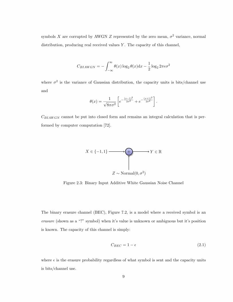
symbols X are corrupted by AWGN Z represented by the zero mean, σ2 variance, normal

distribution, producing real received values Y . The capacity of this channel,

CBIAWGN = −∫ ∞−∞

θ(x) log2 θ(x)dx− 1

2log2 2πeσ2

where σ2 is the variance of Gaussian distribution, the capacity units is bits/channel use

and

θ(x) =1√

8πσ2

[e−

(x−1)2

2σ2 + e−(x+1)2

2σ2

].

CBIAWGN cannot be put into closed form and remains an integral calculation that is per-

formed by computer computation [72].

+

Z ∼ Normal(0, σ2)

Y ∈ RX ∈ {−1, 1}

Figure 2.3: Binary Input Additive White Gaussian Noise Channel

The binary erasure channel (BEC), Figure 7.2, is a model where a received symbol is an

erasure (shown as a “?” symbol) when it’s value is unknown or ambiguous but it’s position

is known. The capacity of this channel is simply:

CBEC = 1− ε (2.1)

where ε is the erasure probability regardless of what symbol is sent and the capacity units

is bits/channel use.

9

0

? Y

1

0

1

X

1− ε

ε

1− ε

ε

Figure 2.4: Binary Erasure Channel

The binary symmetric channel (BSC), Figure 2.5, is model where a received symbol is erred

with a probability p. This channel is used often to model a hard-decision receiver or a

receiver that discretizes the channel information into binary levels. The channel capacity

of this channel is:

CBSC = 1 + p log2 p+ (1− p) log2(1− p)

where p is the probability of a symbol error regardless of what symbol is sent and is in units

of bits/channel use.

0

Y

1

0

1

X

1− p

p

1− p

p

Figure 2.5: Binary Symmetric Channel

10

2.1.2 Burst Error/Erasure

A burst is defined as a localized area of non-zeros in a vector of length n. The burst length

l is defined as the l consecutive symbol positions where the first and the last positions are

non-zero. An error burst would be defined as an error pattern that contains a burst. An

error pattern is a vector of length n where the non-zero elements of the vector indicate the

location of errors. And similarly, an erasure burst is defined as an erasure pattern that

contains a burst. In this case, an erasure pattern is a vector of length n where the non-zero

elements of the vector indicate the location of erasures. In either case, the error/erasure

burst pattern may have zeros within the burst. To specify the requirements for l and n for

a particular application requires statistical knowledge of l and how often the burst reoccurs

to design n. The goal of this thesis is develop codes in which l and n can be easily specified

and burst correction can occur.

11

2.2 Linear Block Codes for Error/Erasure Correction

Linear block codes are used in the Channel Encoder/Decoder blocks of Figure 2.2. A

linear block code C denoted (n, k) is defined as a k-dimension subspace of an n-dimensional

vector space over Galois Field GF(q). In this thesis, we focus on binary GF(2) linear block

codes. Linear block codes can be defined by a k × n generator matrix G = {gi,j} where

i = {0, 1, . . . , k− 1} and j = {0, 1, . . . , n− 1} with a null space defined by an m× n parity-

check matrix H = {hi,j} where i = {0, 1, . . . ,m− 1}, j = {0, 1, . . . , n− 1} and m ≥ n− k.

That is GHT = 0 where T superscript indicates a matrix transpose operation. The matrix

H itself defines a linear block code of length n and dimension n− k. We call this (n, n− k)

code, the dual code of C. It is denoted by C⊥ where the symbol ⊥ superscript indicates

the dual space of C. From this definition, it is clear that all codewords of C are orthogonal

to the codewords of it’s dual.

The G matrix specifies the 2k possible n-tuples or codewords. Any k set of linearly indepen-

dent n-tuples form a basis that span the entire subspace and is used as row specifications

for the G matrix of a code. One particular specification, called a systematic representa-

tion, allows for the codewords to be formed by appending the k information symbols with

n − k parity symbols. This is the result of partitioning the G matrix into two distinct

submatrices: G = [P|Ik] where P is the k × (n − k) parity submatrix and Ik is the k × k

square identity matrix. The systematic representation of G is found from another G matrix

through a series of elementary row operations. This representation is beneficial in encoding,

the process where a codeword is created from a sequence of information symbols which is

defined as a matrix multiplication between a vector u = (u0, u1 . . . , uk−1) of k information

symbols, and the k×n matrix G. By using the systematic representation, the encoding op-

eration is effectively reduced to a matrix multiplication between vector u and the k×(n−k)

submatrix P. Specifically,

v = uG = u [P|Ik] = (uP|u)

12

where v = (v0, v1, . . . , vn−1) denotes the codeword vector. Systematic representation also

assists in the more practical sense. By observing the vector u in v, a fast partial functional

check of an encoder circuit output can be performed.

2.2.1 Cyclic Codes

Cyclic codes are algebraic codes that are defined by polynomial rings over a finite field

[16, 17]. Many important linear block codes have been characterized as cyclic codes, i.e.

Euclidean Geometry; Reed-Solomon; Bose, Ray-Chaudhuri and Hocquenghem (BCH); Go-

lay; and Hamming [18]. They are a much studied subclass of linear block codes since they

can be encoded and decoded with simple shift registers. We define a cyclic shift of i po-

sitions as a positive end around shift (increasing index) of a vector in i positions. Cyclic

codes have the property that the every cyclic shift of a codeword is also a codeword. We

can represent an information vector u and a codeword v as polynomials by defining their

components as coefficients, i.e. u(x) =∑k−1

i=0 uixi and v(x) =

∑n−1i=0 vix

i respectively, where

x is a variable called an intermediate. Then u(x) and v(x) can be related by the following

equation:

v(x) = u(x)g(x) (2.2)

where g(x) =∑n−k

i=0 gixi is called the generator polynomial. If g(x) has degree of n − k

(defined as the largest power of the polynomial) and is a factor of the polynomial xn + 1,

then g(x) generates an (n, k) cyclic code [18]. We can further define a parity polynomial of

degree k as h(x) =∑k

i=0 hixi which is related to the generator polynomial by the following

equation:

h(x) =xn + 1

g(x). (2.3)

It can be shown that the generator polynomial is unique and can be used to create a k× n

generator matrix G by taking the coefficients gi as the first n − k + 1 components of the

13

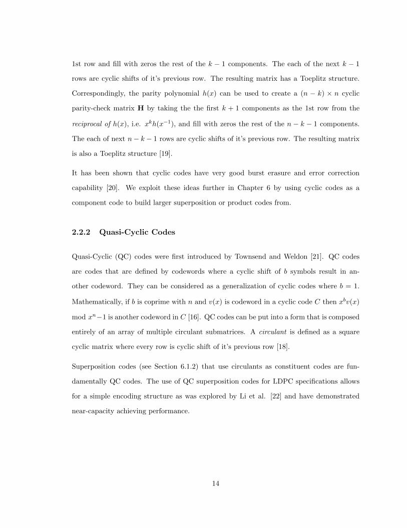
1st row and fill with zeros the rest of the k − 1 components. The each of the next k − 1

rows are cyclic shifts of it’s previous row. The resulting matrix has a Toeplitz structure.

Correspondingly, the parity polynomial h(x) can be used to create a (n − k) × n cyclic

parity-check matrix H by taking the the first k + 1 components as the 1st row from the

reciprocal of h(x), i.e. xkh(x−1), and fill with zeros the rest of the n − k − 1 components.

The each of next n− k − 1 rows are cyclic shifts of it’s previous row. The resulting matrix

is also a Toeplitz structure [19].

It has been shown that cyclic codes have very good burst erasure and error correction

capability [20]. We exploit these ideas further in Chapter 6 by using cyclic codes as a

component code to build larger superposition or product codes from.

2.2.2 Quasi-Cyclic Codes

Quasi-Cyclic (QC) codes were first introduced by Townsend and Weldon [21]. QC codes

are codes that are defined by codewords where a cyclic shift of b symbols result in an-

other codeword. They can be considered as a generalization of cyclic codes where b = 1.

Mathematically, if b is coprime with n and v(x) is codeword in a cyclic code C then xbv(x)

mod xn−1 is another codeword in C [16]. QC codes can be put into a form that is composed

entirely of an array of multiple circulant submatrices. A circulant is defined as a square

cyclic matrix where every row is cyclic shift of it’s previous row [18].

Superposition codes (see Section 6.1.2) that use circulants as constituent codes are fun-

damentally QC codes. The use of QC superposition codes for LDPC specifications allows

for a simple encoding structure as was explored by Li et al. [22] and have demonstrated

near-capacity achieving performance.

14

Chapter 3: Low-Density Parity-Check Codes

3.1 Introduction

LDPC codes are parity-check block codes that have a very low density of non-zero elements

in the parity-check matrix. In his Ph.D. thesis [23], Gallager defined LDPC codes as a class

of linear codes defined entirely by the parity-check matrix with a small constant number

of non-zero elements (or weight) per row compared to the row length and a small constant

weight per column compared to column length [24]. He showed that with high probability

the minimum distance of LDPC codes grows linearly with code length under the condition

that the row weight must be greater than or equal to 3.

Gallager developed two binary iterative decoders. One based on a posteriori probability

(APP) metrics is now known as the sum product algorithm (SPA) for the AWGN channel

(see Section 3.5), and the other, a bit-flipping decoder based on inputs from a binary

symmetric channel (BSC). In order to improve error correction performance of the iterative

decoders, Gallager included a constraint (which we now call the row-column constraint

(RCC) [18]) that no two rows (or columns) have coincident non-zero elements at more

than one column (or row) position of the parity-check matrix. We now call this type

of construction a regular LDPC code to distinguish it from irregular LDPC codes where

the row and column weights are not constant but vary according to distribution functions

called degree distributions [25, 26]. Gallager gave an example semi-random construction

method which showed good error performance for rate=1/2 and 1/4 over an AWGN channel

using the SPA. He also demonstrated LDPC code performance over a Rayleigh fading

channel.

Thirty three years passed between the publication of Gallager’s thesis and it’s rediscovery

15

in 1996 [27, 28] with little attention paid. One exception occurred in 1981 [29]. A graph

representation of the parity-check matrix was introduced by Tanner as a way of analyzing

the iterative behavior of the SPA. This graph representation, which now bares Tanner’s

name, is discussed in more detail in the SPA Section 3.5.

Since it’s rediscovery in 1996, LDPC codes has attracted an enormous attention in the liter-

ature. The first algebraic construction was introduced in 2000 [30] based on Euclidean and

project geometries. This work also gave one of the first successful demonstrations of cyclic

and quasi-cyclic codes using the SPA. In 2001, improved information theoretic tools called

density evolution were introduced to characterize the ensemble error performance based on

the column and row weight distributions of the parity-check matrix, which are called degree

distributions [25, 26, 31]. Density evolution can predict the threshold of convergence of the

iterative decoders in terms of the channel parameter, i.e. a single parameter that describes

the state of the channel. This threshold defines a region of error performance known as

the waterfall region where the errors are reduced at such large exponential rate that error

performance curve resemble a waterfall. By selecting the appropriate degree distributions,

the error performance at the start of the waterfall can be designed and predicted with high

probability without simulations. Using this method, thresholds have been found that reach

0.0045 dB of the AWGN channel capacity [32].

To date, two main methods of LDPC code construction–algebraic construction and semi-

random computer construction, dominate the literature. Each method can be categorized as

either regular and irregular LDPC codes used for asymptotic analysis. While semi-random

computer construction are used for theoretical study, their lack of structure puts a penalty

on integrated circuit routing. Algebraic and other forms of structured LDPC codes on the

other hand allow for more systematic routing thus reducing decoding complexity. In general,

computational decoding complexity is directly proportional to the density of non-zeros in

the parity-check matrix per iteration. The density multiplied by the average number of

iterations define the average computational complexity of a particular LDPC code.

16

3.2 Technical Description

LDPC codes can be categorized by the column and row weight distribution. A regular LDPC

code has constant column weights and constant row weights. An irregular LDPC has vari-

able column weight and variable row weight that is characterized by weight distribution

functions. There can be hybrid structures that have constant column weights with variable

row weights and visa versa that are also categorized as irregular LDPC codes. Character-

izations based on weight functions are used to specify code ensembles rather than specific

codes. Also, analysis based on weight functions pertain to average ensemble behavior and

not a specific instance. Let H define an m×n parity-check matrix that has rank p. Also, let

a regular LDPC code ensemble have row weight of wr and column weight of wc be denoted

as (wc, wr). Then the total number of non-zero elements or 1’s is E = nwc = mwr where the

density of non-zero elements in H is E/(nm) << 0.5. The design rate of a regular (wc, wr)

code is Rd = 1− wc/wr which can be lower than the code rate of R = 1−m/n due to the

possible presence of redundant rows in H. For H to be an LDPC code, we place a further

constraint on the location of the non-zero elements, that is no two rows (columns) can have

more than one column (row) with coincident non-zero components (RCC). It’s purpose will

be made clear when we introduce the Tanner graph in the following passage.

In 1981, Tanner [29] showed that LDPC codes could interpreted as codes operating on a

bi-partite graph, i.e. a graph composed of two types of nodes, variable (VN) and constraint

(CN) that are connected by a network of bi-directional lines or edges. The n VNs represent

each received codeword bit and the m CNs represent every parity-check constraint equation.

The network of edges connecting VNs to CNs are defined by the non-zero elements in parity-

check matrix. For instance, hi,j = 1 for i = 3 and j = 5 would create an edge connecting

VN 5 to CN 3. We define any pair of VN and CN as neighbors if they are connected by an

edge. In this way, no two VNs can be neighbors and the same for any two CNs.

17

V4

C0

V1

V2

V3

V0

C1

C2

Figure 3.1: Tanner Graph Example

H =

1 1 1 0 0

1 0 0 1 1

1 1 0 1 0

. (3.1)

Figure 3.1 shows an example Tanner graph whose associated H matrix is given in (3.1). In

general, the vi nodes are the VNs where i = (0, 1, . . . , n − 1) represent the columns in the

H matrix. The cj nodes are CNs for m ≥ n − k processors associated with each row in

the H where j = (0, 1, . . . ,m − 1) are row indices. The interconnections or edges between

the VNs and CNs are defined by a 1 component in the H and physically define the path

where information or messages are passed between processors. Algorithms that operate

within this structure are called message passing algorithms. A complete iteration is defined

as messages passed from VN to CN and then CN to VN. Information from the channel are

not depicted in Figure 3.1 but they can optionally be shown as a third type of node that are

connected to each VN. They relate to the soft-information samples from the channel which

are considered channel reliabilities since the values are usually in a numerical format with

the sign representing the logic value of the received symbol and the magnitude representing

18

the amount of reliability in the sample.

A connected bi-partitite graph is known from graph theory to have cycles. A cycle is defined

as a complete circuit formed from a starting VN to a series of neighboring edge transversals

through the Tanner graph until it reaches back to the starting VN. We call a cycle of length

n, a cycle of n edge transversals. The girth of a Tanner graph is the smallest cycle length

in the graph. Gallager’s RCC prevents the formation of cycle 4 and therefore all LDPC

codes that conform to this constraint have a girth at least 6. In Section 3.5, we discuss the

impact of cycles on the error performance of LDPC decoding.

An irregular LDPC code can be described as follows. Let λi be the fraction of all edges

that are connected to VN of degree i and let ρj be the fraction of all edges that are

connected CN of degree j. λi and ρj are called the VN and CN distributions respectively

where i = (1, . . . ,m) and j = (1, . . . , n). We note that regular codes are a special case

of irregular codes where | suppλi| = | supp ρj | = 1. A more convenient description of the

weight functions is to define weight polynomials. Let

λ(x) =∑i

λixi−1

ρ(x) =∑j

ρjxj−1

(3.2)

define the column and row degree polynomials respectively. Then an irregular LDPC en-

semble can be denoted as (λ(x), ρ(x)). The design rate of an irregular ensemble is

Rd = 1−∫ 1

0 ρ(x)dx∫ 10 λ(x)dx

. (3.3)

19

For the example graph in Figure 3.1, it has the following pair of degree distributions:

λ(x) =2

8+

6

8x

ρ(x) =2

8x+

6

8x2

with a design rate Rd = 25 .

The significance of the degree distribution description for LDPC ensembles can be seen in

an analytical context. It was proven that with high probability all codes in the ensemble

defined by degree distributions will concentrate it’s asymptotic (i.e. for an infinite block

code or the case of a Tanner graph free of cycles) performance around the average ensemble

performance [31]. Furthermore, the ensemble performance of LDPC codes with message

passing can be characterized by it’s decoding threshold. This is point where the decoder

will converge to the correct answer with very high probability. Or more precisely, the

decoding threshold is the maximum channel parameter such that for all channel parameters

strictly less than this value, the expected fraction of incorrect messages approaches zero

as the number of iterations increases. The channel parameter is defined as a variable that

characterizes the state of the channel (from Section 2.1), i.e. σ2 for a BIAWGN channel, ε for

a BEC channel and p for the BSC. One method of calculating the decoding threshold is called

density evolution [31, 33]. Density evolution analyzes, through numerical computation, the

evolving probability distribution functions (PDF) of messages passed between VN and CN

as the decoder iterations grow toward infinity. The PDF will eventually converge to a fixed

distribution where a non-negative PDF indicates the presence of errors and whose mean is

a function of the channel parameter. For the BEC, closed form solutions for the decoding

threshold exists. Let the decoding threshold be defined as ε∗ = sup{ε : f(ε, x) < x,∀x ≤ ε},

where f(ε, x) = ελ(1 − ρ(1 − x)) is derived from the average probability (or density) of

20

erasures at each node at one iteration [34,35]. For the case of regular ensembles,

ε∗ =1− s

(1− swr−1)wc−1(3.4)

where s is the positive root of [(wc − 1)(wr − 1)− 1] ywr−2 −∑wr−3

i=0 yi = 0. It has been

shown that for a (3, 6) LDPC ensemble where R = 1 − wc/wr = 0.5, ε∗ = 0.4294 [34].

Equation (2.1) says that when at capacity, R = CBEC and ε = 1 − R = 0.5. Therefore, a

(3, 6) LDPC code ensemble performs within ε − ε∗ = 0.0706 of capacity. This small rate

loss is the result of using a regular ensemble. It was shown in [36,37] that irregular LDPC

ensembles can be design to perform arbitrarily close to the BEC capacity.

In practice, the decoding threshold accurately predicts the onset of decoding convergence

for the message passing decoder at high BER region even for finite length block sizes. It

has not been understood why this is so. What density evolution fails to do is predict how

the decoder will work at low BER. For this region, different tools have been developed for

finite block sizes. For the BEC channel, a phenomena known as stopping sets dominate

the error performance at this region. A stopping set S is a subset of the VNs such that

all neighbors of S are connected to S at least twice [35]. If an erasure pattern occurs with

erasures positioned at every member of a stopping set, the message passing decoder will

fail to correct this pattern. This is because neighboring CNs of the stopping set will always

have at least two erasures to resolve regardless of the number of iterations. We discuss the

message passing algorithm for the BEC in detail in Section 3.7.

3.3 LDPC Code Construction

This section describes various methods of constructing LDPC codes.

21

3.3.1 Mackay Codes

Mackay’s random construction of LDPC codes gives a near-regular ensemble. Define a m×n

parity-check matrix H that is created at random with a constant weight per column of t so

that the row weights are constant or nearly constant. Also, we observe Gallager’s RCC by

allowing no more than one location of coincident 1’s of any pair of rows (columns). Mackay

suggested an alternate of methods of generating regular codes by using smaller permutation

submatrices, which are row or column permutations of an identity matrix, to form larger

parity-check matrices–a technique that is a form of superposition code construction (Section

6.1.2). He also found that regular construction LDPC were limited to how close they could

approach the channel capacity and suggested an irregular construction to achieve better

performance. By adding m/2 weight 2 columns to H in a dual diagonal form (or two

identity matrices) to avoid low weight codewords, he demonstrated improved performance

over regular construction. In all instances, the adherence to the RCC was maintained.

3.4 Structured LDPC Codes

One of our primary objective for this dissertation is to explore structured LDPC codes.

Therefore in this section, we present a number of approaches for LDPC code design.

3.4.1 Euclidean Geometry Codes

Euclidean geometry (EG) codes are based on points that are incident to lines or hyperplanes

(flats) defined by a specific finite geometry [18]. Consider a finite field GF(2sp) where s and

p are integers. This finite field structure can also be considered an p-dimensional Euclidean

geometry EG(p, 2s) where points are defined as vectors or p-tuples over elements from

GF(2s) and the all-zero p-tuple defines the origin. Let βi represent an element of GF(2s).

Let a1 and a2 be two linearly independent points, i.e. a1β1 + a2β2 6= 0. A set of 2s points

22

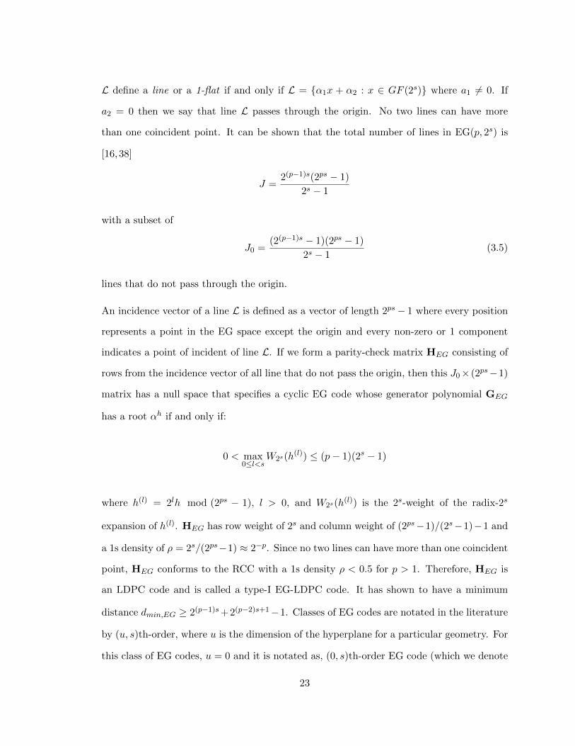
L define a line or a 1-flat if and only if L = {α1x + α2 : x ∈ GF (2s)} where a1 6= 0. If

a2 = 0 then we say that line L passes through the origin. No two lines can have more

than one coincident point. It can be shown that the total number of lines in EG(p, 2s) is

[16, 38]

J =2(p−1)s(2ps − 1)

2s − 1

with a subset of

J0 =(2(p−1)s − 1)(2ps − 1)

2s − 1(3.5)

lines that do not pass through the origin.

An incidence vector of a line L is defined as a vector of length 2ps − 1 where every position

represents a point in the EG space except the origin and every non-zero or 1 component

indicates a point of incident of line L. If we form a parity-check matrix HEG consisting of

rows from the incidence vector of all line that do not pass the origin, then this J0× (2ps−1)

matrix has a null space that specifies a cyclic EG code whose generator polynomial GEG

has a root αh if and only if:

0 < max0≤l<s

W2s(h(l)) ≤ (p− 1)(2s − 1)

where h(l) = 2lh mod (2ps − 1), l > 0, and W2s(h(l)) is the 2s-weight of the radix-2s

expansion of h(l). HEG has row weight of 2s and column weight of (2ps−1)/(2s−1)−1 and

a 1s density of ρ = 2s/(2ps−1) ≈ 2−p. Since no two lines can have more than one coincident

point, HEG conforms to the RCC with a 1s density ρ < 0.5 for p > 1. Therefore, HEG is

an LDPC code and is called a type-I EG-LDPC code. It has shown to have a minimum

distance dmin,EG ≥ 2(p−1)s+2(p−2)s+1−1. Classes of EG codes are notated in the literature

by (u, s)th-order, where u is the dimension of the hyperplane for a particular geometry. For

this class of EG codes, u = 0 and it is notated as, (0, s)th-order EG code (which we denote

23

as C(1)EG(p, 0, s)) prior to it’s rediscovery as an LDPC code [18,30].

For the special case of p = 2, C(1)EG(2, 0, s) gives a square cyclic HEG matrix (circulant) of

dimension (22s − 1)× (22s − 1). The code has length n = 22s − 1, dimension k = 22s − 3s,

and number of parity bits n− k = 3s − 1. It’s minimum distance has shown to be exactly

dmin,EG = 2s + 1 and it’s error performance has been studied many times for the SPA

[18,30,39]. We shall use this code as component codes for our research of burst-erasure and

burst-correction codes in Chapter 6 since it has many good robust properties such as good

minimum distance, many decoding options besides the SPA, and is easy to encode.

3.4.2 Product Codes

Product codes were introduced by Elias in 1954 [40]. The technique consist of creating a

large code out of smaller component codes using a tensor (or Kronecker) product of their

generator matrices. Mathematically, we start by defining two-dimensional product codes,

however, it is not difficult to extend this to dimensions greater than two.

Definition: For t = 1 and 2, let Ct(nt, kt) denote a component linear block code of length

nt and dimension kt of a two-dimensional product code CP .

Let Gt =[g

(t)i,j

]be the generator matrix of Ct. For a two dimensional Product Code C1×C2

with component codes C1 and C2, the product code generator matrix GP of dimension

k1k2 × n1n2 can be defined as:

GP = G2 ⊗G1 =

(G1g

(2)i,j

)(3.6)

where ⊗ is the Kronecker Product [41]. If we switch G1 with G2, we get another code that

is combinatorially equivalent. As can be seen from (3.6), the product code can be seen as a

24

special case of superposition codes (see Section 6.1.2) where the non-zero or 1 elements of

G2 are replaced by a submatrix defined by G1 and the 0 elements of G1 are replaced with

a zero matrix of dimensions G1. The generator matrix GP can be used to encode using

conventional linear block code means (see Section 2.2).

25

3.5 Sum Product Algorithm

The SPA was historically discovered independently by many researchers. It’s first discovery

is attributed to Gallager [24] who developed a probabilistic algorithm based on iteratively

estimating the APP of a received symbol. It’s title can be attributed to a 1996 thesis

by Wiberg [27] who was one of the researchers credited with it’s rediscovery. In 1988,

Pearl discovered an algorithm for machine learning based also on an iterative calculation

of APP over graphs [42]. This algorithm is called Pearl’s Belief Propagation (BP) and was

independently discovered around the same time by others [43, 44]. In 1995, Mackay and

Neal applied BP based decoding to their random construction of LDPC codes and showed

good performance in a BSC channel [45]. However, the authors failed to recognize that the

SPA is in fact an application of BP. They wrongly thought that the SPA algorithm was the

Meier and Staffelbach algorithm of belief networks [46]. The mistake was later identified

and it was proved that the SPA is an instance of BP for error correction coding [47, 48].

In 1999, Mackay showed that the error performance of his randomly constructed LDPC

codes and Gallager’s LDPC codes approached the channel capacity for AWGN channels

[49].

The SPA is based on iteratively estimating the APP of a received bit is a 1 conditioned on

the satisfying of the set of parity-check equations it is checked to and the received channel

information. Let’s define the xd as the value of the transmitted bit and at position d where

d ∈ {0, 1, . . . , n−1}. We call a bit position j checked by a row i, if and only if hi,j 6= 0, where

hi,j is defined as the components of the parity-check matrix H. For a particular received

bit, this calculation can be viewed as tree structure. That is, a received bit is checked

by a number of rows according to the non-zero column components in it’s bit position of

the parity-check matrix. Since every row is a parity-check equation that checks other bit

positions, the computation can become intractable as you progress through each tier of

the tree. Gallager recognized that the APP calculation could be made to fold onto itself at

every level of the tree creating a process that cycles or iterates. For a particular received bit,

26

this was accomplished by eliminating it’s own APP from the prior iteration to estimate it’s

current APP. This approach created multiple processing units that could work in parallel.

However, the artificial folding in the algorithm creates an approximation to the APP or a

false APP and thus sub-optimal decoding performance.

The SPA is generally defined in the log-likelihood domain. Specifically, assuming binary

transmissions where x is a binary symbol, x ∈ {0, 1}, a transmitted sequence of n symbols

is mapped using y = (1−2x), where y ∈ {−1, 1} then the received symbol is r = y+z where

r ∈ R and z is assumed to be additive white Gaussian noise (or the BIAWGN channel).

Define the log-likelihood ratio as: LLR(r) = log P (x=1|r)P (x=0|r) = 2

σ2 r. Using the terminology

from Section 3, let Si be the set of CNs connected to VN vi. Let Si\j define the set of CNs

connected to VN vi except CN cj . (Refer to Figure 3.1.) Let Ti\j define the set of VNs

connected to CN ci except VN vj . Also let λi→j be defined as the message passed from vi

to cj and γj→i be defined as the message passed from cj to vi. Then we can define the LLR

domain SPA as:

1. Perform LLR conversion of channel information: LLR(ri) = 2σ2 ri where i = (0, 1, . . . , n−

1).

2. VNs vi pass messages λi→j = LLR(ri) to CNs cj .

3. CNs cj pass messages γj→i = 2 tanh−1(Πl∈Ti\j tanh (λl→j/2)) to VNs vi.

4. VNs vi pass messages λi→j = LLR(ri) + Σl∈Si\jγl→i to CNs cj .

5. If a fixed number of iterations has occurred, output estimated x̂ or if a syndrome

check (x̂HT = 0) indicates that x̂ is a codeword, stop, else goto 3.

Note: to find x̂, define the log of the false APP ratio estimates: LFAR(ri) = LLR(ri) +

27

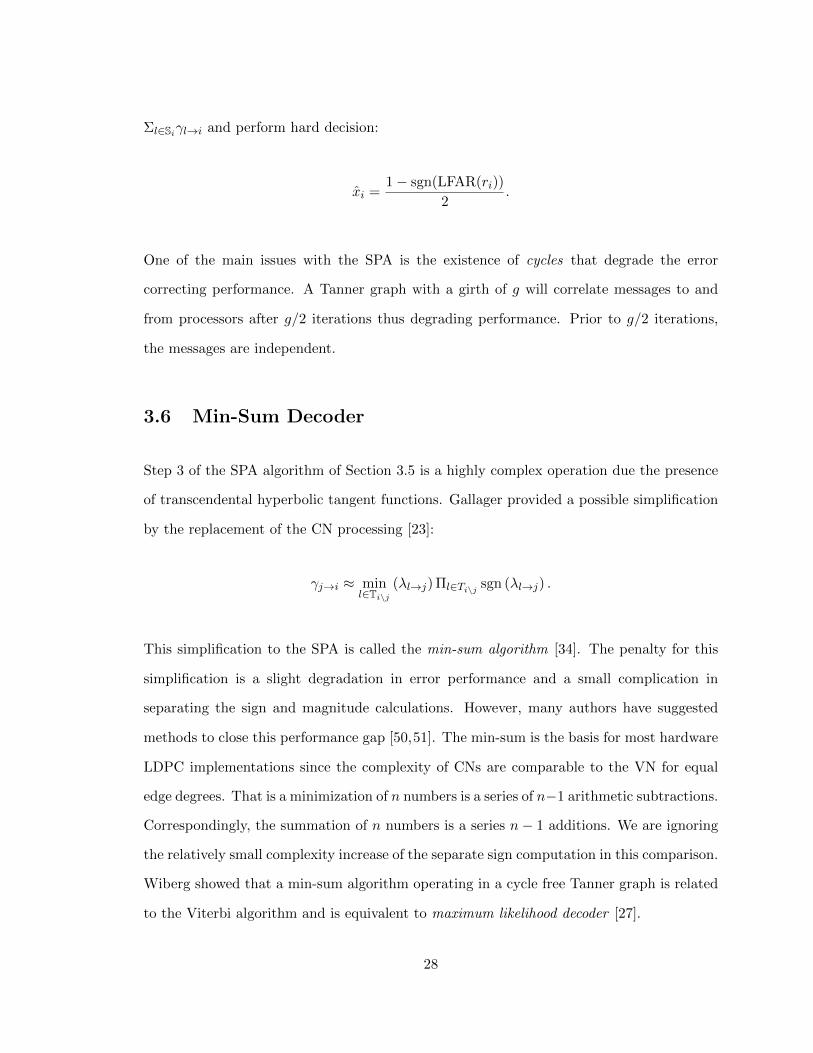
Σl∈Siγl→i and perform hard decision:

x̂i =1− sgn(LFAR(ri))

2.

One of the main issues with the SPA is the existence of cycles that degrade the error

correcting performance. A Tanner graph with a girth of g will correlate messages to and

from processors after g/2 iterations thus degrading performance. Prior to g/2 iterations,

the messages are independent.

3.6 Min-Sum Decoder

Step 3 of the SPA algorithm of Section 3.5 is a highly complex operation due the presence

of transcendental hyperbolic tangent functions. Gallager provided a possible simplification

by the replacement of the CN processing [23]:

γj→i ≈ minl∈Ti\j

(λl→j) Πl∈Ti\j sgn (λl→j) .

This simplification to the SPA is called the min-sum algorithm [34]. The penalty for this

simplification is a slight degradation in error performance and a small complication in

separating the sign and magnitude calculations. However, many authors have suggested

methods to close this performance gap [50,51]. The min-sum is the basis for most hardware

LDPC implementations since the complexity of CNs are comparable to the VN for equal

edge degrees. That is a minimization of n numbers is a series of n−1 arithmetic subtractions.

Correspondingly, the summation of n numbers is a series n− 1 additions. We are ignoring

the relatively small complexity increase of the separate sign computation in this comparison.

Wiberg showed that a min-sum algorithm operating in a cycle free Tanner graph is related

to the Viterbi algorithm and is equivalent to maximum likelihood decoder [27].

28

3.7 Erasure Correcting Algorithm

The erasure correcting algorithm (ERA) for binary LDPC codes was defined by Luby et

al. [52]. This algorithm, for random erasure correction, is described as follows. Let hi,j

represent the components of the parity-check matrix H where i = (0 . . .m − 1) and j =

(0 . . . n−1). Let yj represent the received codeword. Let K = {j|yj =?} where ? is a symbol

for a received erasure. K is the set of all received erasure symbol positions in the codeword.

By definition of the parity-check matrix,

∑j

yjhi,j = 0 (3.7)

for any row i. Recall that a column j (or bit position) is checked by a row i, if and only if

hi,j 6= 0. If there exist a row t where only one element k ∈ K is checked then by (3.7):

yk =∑j 6=k

yjht,j . (3.8)

Now the decoding algorithm can be defined. Identify a subset L of K where every element

of L is an erasure position that is checked by a row that checks no other erasure. Correct

every element in L using (3.8), and remove them from K. Then iterate the entire algorithm

repeatedly until there are no elements in K or no elements in L can be identified but K

is not empty. In the former case, the decoding is successful and in the latter case, the

decoding fails. This thesis utilizes this simple burst-erasure correcting algorithm as guide

to construct LDPC type of codes.

This section concludes the background portion of this thesis. The rest of the dissertation is

devoted to the research results in Chapters 4 and 6. Then Chapter 8 concludes with final

remarks.

29

Chapter 4: Burst Erasure Correction Ensemble Analysis for

Random LDPC Codes

4.1 Introduction

Burst erasure correction is a subject of research which has seen many applications. It can

be applied to fields such as correcting atmospheric fades from laser communications [53] or

packet losses in a network [54]. Recent research to the general problem of burst erasure

correction can be found in [1–3]. In [55, 56], the articles presented a new application of

a recursive erasure correction algorithm of low complexity based on the distribution of

consecutive zeros in the parity-check matrix for a cyclic code. We refer to this algorithm as

the RED algorithm, a modification of the ERA algorithm. These articles recognized that

a burst of erasures can be corrected symbol-by-symbol as long as for every position within

the residual burst erasure pattern, a row in the parity-check matrix can be found that will

check that particular position and no other position within the residual burst.

Song et. al. [56] developed an analysis tool to quantify a parity-check matrix’s capacity to

correct a guaranteed minimum burst length. They defined a zero-span as a contiguous string

of zeros between two unique non-zero entries indexed from the position of the first non-zero

entry to the second non-zero entry. By this definition, a Zero-covering span profile, denoted

δ = {δl}, is defined as the largest zero-span at column position l over all rows of the parity-

check matrix H, where l ∈ {0, . . . , N − 1} and N is the block length. Then the guaranteed

burst erasure correcting capability while using the RED algorithm can be defined by δ + 1

where δ = min{δl} which is called the Zero-covering span of H. Tai et. al [55] focused on

Euclidean geometry based cyclic and dispersed quasi-cyclic codes as they recognized that

such codes have a consistent zero-covering span over all column positions.

30

In [57, 58], the authors extended the prior analysis in a more detailed approach when an-

alyzing a general parity-check matrix. It was discovered that the erasure burst correction

capability for a general parity-check matrix using RED is defined by it’s Correctible profile

γ = {γl} where l ∈ {0, . . . , N − 1}. This profile specifies the largest burst length that

the RED algorithm can correct recursively before a stopping condition is encountered, i.e.

no rows can be found at the current erased position with a zero-span that is greater than

the current burst erasure length minus one. In other words, there must a large enough

zero-span to mask out all erasures except for the current target erased symbol. Therefore

the Correctible profile γ is the measure of the true burst erasure correction capability using

the RED algorithm while the Zero-covering span profile δ, represents the potential burst

erasure correction capability.

This thesis will expand on the ideas of [57,58] by analyzing the zero-spans for the ensemble

of randomly generated LDPC matrices. Typically for a general parity-check matrix, δ and

γ are difficult to mathematically characterize. This problem is overcome by considering the

statistical characterization of the ensemble of random codes. The goal of this thesis is to

statistically characterize both the δ and the γ of the ensemble of random LDPC codes with

parity-check matrices of constant column weights. We answer the question of whether it is

possible to find the average ensemble performance. The probability mass function (PMF)

of both the Zero-covering span profile {δl} and the Correctible profile {γl} are derived and

data is provided for 100, 1, 000 and 10, 000 bit blocks to demonstrate the accuracy of the

analysis. The moments for both PMFs, δ and γ, are presented for various column weights,

e.g. 2 to 8 and various blocks sizes, e.g. 100, 1, 000 and 10, 000 bits. The means of the γ

PMFs are calculated for various coding rates and column weights. For smaller block sizes,

the use of truncated PMFs for δ and γ provide more accurate results, however, there is

an increased likelihood of rows containing all zeros. This can potentially skew the results.

The limitations of the analysis are explored and the appropriate regions where the analysis

are applicable are defined. An alternative to this approach is to simply define an ensemble

where the parity-check matrix does not contain the all zero row and rows which contain

31

a single non-zero. The latter is due to the fact that a single non-zero is not a complete

zero-span and therefore it cannot be considered as a potential row in the RED algorithm.

This ensemble is called the expurgated ensemble in this thesis. This is also analyzed in

detail with examples of block sizes of 100, 1, 000 and 10, 000 bits provided. It is shown with

computer generated data, that all statistical predictions are accurate. Finally, we will prove

that the ensemble mean performs asymptotically well as the block size approach infinity.

That is random LDPC codes are asymptotically good for burst erasure correction using the

RED algorithm.

32

4.2 Zero-Span Characterization for Random LDPC Codes

4.2.1 Background

The RED algorithm for burst erasure correction consists of correcting the first erasure in

the burst by identifying a row in the parity-check matrix that has a non-zero entry at that

erased position and zeros entries at the other erased positions. The zeros mask out the other

erasures while isolating the target erasure. Correct this erased position by solving for it’s

value, i.e. one row equation and one unknown symbol. Once the first erasure is corrected,

then others are corrected recursively in sequential order through the same process. This is

explained in detail in the next section.

4.2.2 Recursive Erasure Decoding

From [55,56], the ERA algorithm, (see Section 3.7), was modified slightly to correct symbol-

by-symbol erasure bursts, which we call the RED algorithm. If a burst of v consecutive

erasures starts at the kth column position and ends at the (k + v − 1)th column, contains

all of the elements in the set K, a row t in the parity-check matrix can be identified that

has a non-zero element at k and zeros at (k + 1, . . . , k + v − 1). Then (3.8) is guaranteed

to solve for the erased value. Afterwards, a residual erasure burst of length v − 1 remains.

Through recursion, the next erasure at column position k + 1 as well as the rest of the

burst can be corrected or until a stopping condition occurs, i.e. no row t can be identified

that has a non-zero entry at the current target erasure and zeros at the remaining burst

positions. If no stopping condition is encountered during recursion and all erasures are

corrected then the burst erasure correction capability at column position k is at least v

otherwise if a stopping condition is encountered at column position k + w and w < v then

the burst erasure correction capability at column position k is w.

The characterization of the burst erasure correction capability, i.e. the largest burst erasure

33

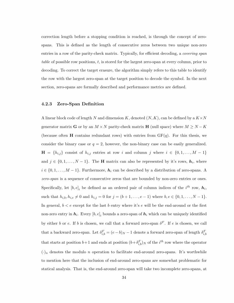
correction length before a stopping condition is reached, is through the concept of zero-

spans. This is defined as the length of consecutive zeros between two unique non-zero

entries in a row of the parity-check matrix. Typically, for efficient decoding, a covering span

table of possible row positions, t, is stored for the largest zero-span at every column, prior to

decoding. To correct the target erasure, the algorithm simply refers to this table to identify

the row with the largest zero-span at the target position to decode the symbol. In the next

section, zero-spans are formally described and performance metrics are defined.

4.2.3 Zero-Span Definition

A linear block code of lengthN and dimensionK, denoted (N,K), can be defined by aK×N

generator matrix G or by an M ×N parity-check matrix H (null space) where M ≥ N −K

(because often H contains redundant rows) with entries from GF(q). For this thesis, we

consider the binary case or q = 2, however, the non-binary case can be easily generalized.

H = {hi,j} consist of hi,j entries at row i and column j where i ∈ {0, 1, . . . ,M − 1}

and j ∈ {0, 1, . . . , N − 1}. The H matrix can also be represented by it’s rows, hi, where

i ∈ {0, 1, . . . ,M − 1}. Furthermore, hi can be described by a distribution of zero-spans. A

zero-span is a sequence of consecutive zeros that are bounded by non-zero entries or ones.

Specifically, let [b, e]i be defined as an ordered pair of column indices of the ith row, hi,

such that hi,b, hi,e 6= 0 and hi,j = 0 for j = (b+ 1, . . . , e− 1) where b, e ∈ {0, 1, . . . , N − 1}.

In general, b < e except for the last b entry where it’s e will be the end-around or the first

non-zero entry in hi. Every [b, e]i bounds a zero-span of hi which can be uniquely identified

by either b or e. If b is chosen, we call that a forward zero-span δF . If e is chosen, we call

that a backward zero-span. Let δFi,b = (e− b)N − 1 denote a forward zero-span of length δFi,b

that starts at position b+1 and ends at position (b+δFi,b)N of the ith row where the operator

(·)n denotes the modulo n operation to facilitate end-around zero-spans. It’s worthwhile

to mention here that the inclusion of end-around zero-spans are somewhat problematic for

statical analysis. That is, the end-around zero-span will take two incomplete zero-spans, at

34

the end and at the beginning of a row, and form a complete zero-span, creating potentially

a zero-span that is not consistent with analysis. This could skew the data away from the

analysis. We will present evidence of this effect when the analysis is compared with data

for small block sizes in Section 5.

Continuing with the analysis, we will now define an entry in the forward Zero-covering span

profile δF as:

δFb = maxiδFi,b.

And similarly, let δBi,e = (e−b)N−1 denote a backward zero-span of length δBi,b that starts at

position e− 1 and ends at position (e− δBi,b)N of the ith row where the modulo n operation

facilitates end-around zero-spans. We can now define an entry in the backward Zero-covering

span profile δB as:

δBe = maxiδBi,e.

Since the b and e are general column indexes, δFb and δBe will now be referred to as δFl and

δBl where l ∈ {0, 1, . . . , N − 1}. (For a cyclic code, δFl and δBl are consistent and equivalent

as shown in [55,56].)

The Zero-covering span profiles, δF and δB, do not determine the burst erasure correcting

ability of the RED algorithm since it does not take into account the possibility of the

stopping condition occurring. It does give a precise indication of the largest burst that

can be considered for correction that starts at a particular column position. Therefore, it

provides an upper bound on the best burst erasure correction capability. The true burst

erasure correction capability is specified by the Correctible profile γF = {γFl } defined by

[57, 58] in Proposition 1 and summarized below. It is a specification of the largest burst

erasure can be corrected at every column position l ∈ {0, 1, . . . , N − 1} with the RED

algorithm.

35

From [57,58], the following proposition was presented:

Proposition 1: Let H be an M × N parity-check matrix of an (N,K) linear block code

over GF(q) with forward Zero-covering span profile δF = {δF0 , δF1 , . . . , δFN−1} and back-

ward Zero-covering span profile δB = {δB0 , δB1 , . . . , δBN−1}, then the following is true for

l ∈ {0, 1, . . . , N − 1}:

1. γFl is the maximum integer for which δF(l+j)N ≥ γFl − j − 1 for j = (0, 1, . . . , γFl − 1).

2. γBl is the maximum integer for which δB(l+j)N ≥ γBl − j − 1 for j = (0, 1, . . . , γBl − 1).

3. γFBl is the maximum integer for which there is a sequence (l′t, l′′t ) of pairs of integers

where t = (0, 1, .., γFBl − 1), such that l′0 = l and l′′0 = (l + γFBl − 1)n and, for each

t ≥ 1, either l′t = l′t−1 +1, l′′t = l′′t−1, and δFl′t−1≥ (l′′t−1− l′t−1)n or l′t = l′t−1, l′′t = l′′t−1−1,

and δBl′t−1≥ (l′′t−1 − l′t−1)n.

Note the third item in Proposition 1: γFBl are entries in a forward-backward Correctible

profile, defined in [57] but is not included in this analysis. Also, from this point on, since

the analysis for the δF and δB are the same, references to δB are implied and no longer

typed whenever δF is indicated.

Also, the RED algorithm can be implemented in parallel, if for γFl , an additional condition

is included in Proposition 1: δB(l+j)N ≥ j. That is, there must a large enough backward

zero-covering span at (l+ j)N to mask out the other erasures in the burst. If γFl is defined

in this manner, it is possible that the γFl from Proposition 1, is reduced. It maybe possible

that with more structured codes, such as cyclic codes, that this reduction is minimized.

The same approach can be considered for γBl in Proposition 1.

To illustrate the concept of Zero-covering span profile δF and Correctible profile γF , (4.1)

36

below shows an example of a 7×15 parity-check matrix of constant column weight 4.

H =

0 1 1 0 1 1 0 0 0 1 1 1 1 0 0

1 0 0 1 1 0 1 0 1 1 0 0 1 0 1

0 0 0 1 1 1 1 1 0 0 0 0 0 1 1

1 1 1 1 1 0 0 1 1 1 1 0 0 0 0

0 1 1 0 0 0 1 1 1 0 0 1 1 1 0

1 0 1 1 0 1 1 0 1 0 1 1 1 1 1

1 1 0 0 0 1 0 1 0 1 1 1 0 1 1

. (4.1)

The corresponding Zero-covering span profile δF of the example is given as:

δF =(

2 3 3 1 2 3 1 5 2 2 4 1 3 2 3). (4.2)

And the corresponding Correctible profile γF is given as:

γF =(

3 4 3 2 3 3 2 4 3 3 3 2 4 3 4). (4.3)

We note a few observations. Referencing the column position with index l ∈ {0, 1, . . . , 14},

there are only four positions: 2, 5, 7, and 10; where the Correctible profile γFl is not one

greater than the corresponding Zero-covering span profile δFl . As stated in Proposition 1,

the succeeding δFl values determine the Correctible profile γFl . For instance, to achieve

γF2 = 4 for δF2 = 3, δF2 must be followed by, at a minimum, δF3 = 2, δF4 = 1 and δF5 = 0.

However, δF3 = 1, δF4 = 2, and δF5 = 3. Therefore, δF3 is one less than required and so γF2 is

3. For this example most of Correctible profile γFl = 1 + δFl . However, we will show as the

block size gets larger for the ensemble of random LDPC codes with parity-check matrices

of constant column weight, the mean δFl > mean γFl .

The Correctible profile γFl is difficult to work with in it’s form specified in Proposition 1. In

37

order to facilitate its analysis, we will need to transform it’s definition to find γFl directly.

This is achieved in the next section as part of the overall analysis of zero-spans.

Figures 4.1 and 4.2 show the statistical data collected of a (240,160) randomly generated

LDPC matrix of constant column of 3 for the Zero-covering span profile and the Correctible

profile. In both cases, there are large differences between the potential burst correction

capability of δFl + 1 and δBl + 1, and it’s corresponding true Correctible profile γFl and γBl .

This shown in the bottom plots of Figures 4.1 and 4.2. Both plots show that as much as a

difference of 140 bits can exist.

Figures 4.3 and 4.4 show the scatter plot and the histogram of the LDPC code used in

Figures 4.1 and 4.2. Note that Figure 4.4 appears to be a positively skewed distribution,

i.e. lower zero-covering span values have a higher frequency of occurrences [59]. In the

next section, data is analyzed of different blocks sizes and various column weights and the

predictions of the ensemble Zero-covering span profile PMF are developed. Also analyzed is

the data collected for γBl and this data is also predicted by the ensemble Correctible profile

PMF in Section 4.3.3.

To compare these results to a cyclic code (and to validate our software), we select the

Euclidean Geometry C(1)EG(2, 0, 4) (255,175) LDPC code based on EG(2, 24). This code has

constant row and column weights of 16. It’s minimum distance has been shown to be 17.

Applying the measures according to Proposition 1, we achieve the following results shown

in Figures 4.5, and 4.6 with a scatter diagram of the parity-check matrix in Figure 4.7.

The results confirm that a cyclic code has a constant erasure burst correcting capability

with δFl = δBl = 54 and γFl = γBl = 55; and that it achieves the ideal performance

criteria: γFl = δFl + 1 = 56 and γBl = δBl + 1 = 56. And that although both codes are of

similar length, the cyclic code is better in burst erasure correction capability based on the

algorithms discussed.

In summary, this section introduces the recursive erasure decoding and it formally defines

38

0 50 100 150 200 2500

50

100

150!F is the max forward zero span at each column index

0 50 100 150 200 2500

20

40"F is the max forward erasure correcting capability

0 50 100 150 200 2500

50

100

150(!F + 1) −"F

Figure 4.1: (240,160) Randomly Generated LDPC Code Forward Zero-Covering Span Pro-file and Forward Correctible Profile

the zero-span and it’s relationship to the important Zero-covering span profile δFl . The

Correctible profile γFl is also defined from Proposition 1 [57, 58] and specifies the true

erasure burst correction capability of the RED algorithm. The next section begins the

statistical analysis of the PMFs of δFl and γFl for the ensemble of randomly generated

LDPC codes.

4.3 Statistical Analysis for the General Ensemble of Random

LDPC Codes

Let H = {hi,j} represent a parity-check matrix of a (N,K) binary LDPC code where the

columns are of constant weight λ, 0 ≤ i < M , M ≥ N −K and 0 ≤ j < N . Let δFi,j be a

39

0 50 100 150 200 2500

50

100

150!B is the max backwards zero span at each column index

0 50 100 150 200 2500

10

20

30"B is the max backwards erasure correcting capability

0 50 100 150 200 2500

50

100

150(!B + 1) −"B

Figure 4.2: (240,160) Randomly Generated LDPC Code Backward Zero-Covering SpanAnalysis and Backward Correctible Profile

0 50 100 150 200

0

20

40

60

80

nz = 720

Scatter Chart of Matrix

Figure 4.3: (240,160) LDPC Code Scatter Plot

40

0 50 100 1500

1

2

3

4

5

6

7

Forward Zero Span Length

Num

ber o

f Col

umn

Indi

ces

Histogram of !F

Figure 4.4: (240,160) LDPC δF Histogram

0 50 100 150 200 250 30053

54

55!F is the max forward zero span at each column index

0 50 100 150 200 250 30054

55

56"F is the max forward erasure correcting capability

0 50 100 150 200 250 300−1

0

1(!F + 1) −"F

Figure 4.5: EG (255,175) LDPC Code Forward Span Analysis

41

0 50 100 150 200 250 30053

54

55!B is the max backwards zero span at each column index

0 50 100 150 200 250 30054

55

56"B is the max backwards erasure correcting capability

0 50 100 150 200 250 300−1

0

1(!B + 1) −"B

Figure 4.6: EG (255,175) LDPC Code Backward Span Analysis

0 50 100 150 200 250

0

50

100

150

200

250

nz = 4080

Scatter Chart of Matrix

Figure 4.7: EG (255,175) LDPC Code Scatter Plot

42

random variable (RV) whose value is the forward zero-span at row i ∈ {0, 1, . . . ,M−1} and

starting at column position j ∈ {0, 1, . . . , N − 1} given that hi,j = 1. Let the probability

p = Pr(hi,j = 1) = λM then Pr(hi,j = 0) = 1− p =

(1− λ

M

). Then

PδFi,j |hi,j(δ|hi,j = 1) = p(1− p)δ =

λ

M

(1− λ

M

)δ(4.4)

is a geometric PMF under the assumption is that the probabilities p are independent

Bernoulli variables. The mean is well-known [60] and it’s value is:

µδFi,j=

1− pp

=1− λ

MλM

. (4.5)

The goal is to find the forward Zero-covering span profile PMF for δFj = maxx δFx,j , where

x = {i|hi,j = 1} and |x| = λ. We note that since all zero-spans are conditioned on hi,j = 1

at the starting position, all distributions are also conditioned on hi,j = 1 for the starting

position. Therefore, for efficient notation, the conditioning is assumed for the rest of this

chapter.

The PMF of the maximum of λ multiple independent identically distributed (IID) RVs, Vt,

is known [61]: if Z = max{V1, V2, . . . , Vλ} then the probability that the RV Z takes on a

value b is given by: PZ(b) = FV (b)λ − FV (b− 1)λ where FV is the cumulative distribution

function (CDF) of V and V is defined as any of the Vt for 0 < t ≤ λ since all Vt are IID.

Therefore,

PδFj(δ) =

[FδFi,j

(δ)]λ−[FδFi,j

(δ − 1)]λ

=

[δ∑

k=0

PδFi,j(k)

]λ−

[δ−1∑k=0

PδFi,j(k)

]λ.

43

The subscript j can be dropped since the PMF is not dependent on the initial column

position. Then the summation is a finite geometric series, and therefore

PδF (δ) =

[δ∑

k=0

p(1− p)k]λ−

[δ−1∑k=0

p(1− p)k]λ

=

[1−

(1− λ

M

)δ+1]λ−

[1−

(1− λ

M

)δ]λ,

(4.6)

since for a geometric series [62]∑n

k=0 rk = 1−rn+1

1−r .

To demonstrate the validity of (4.6), we plot the histograms of the ensemble average of the

zero-covering spans of 1000 randomly generated constant column weight LDPC matrices

of dimension 80× 2000 in Figure 4.8. The graph clearly shows a strong curve relationship

between the prediction by (4.6) and the computer generated data. We note that (4.6)

does not include RCC conformance. This is because the RED algorithm is not an iterative

decoding and does not directly benefit from the RCC constraint.

4.3.1 Moments of the Zero-Covering Span PMF

The mean µδF of δF 4.6 is defined as:

µδF =

N−2∑δ=0

δPδF (δ)

=

N−2∑δ=0

δ

[

1−(

1− λ

M

)δ+1]λ−

[1−

(1− λ

M

)δ]λ ,

where δ range from 0 to N − 2 because the largest zero-span that occur is N − 2 since the

minimum row weight is 2 for a zero-span.

44

0 50 100 150 200

5

10

15

20

25

30

35

40

Forward Zero Span Length

Fre

qu

en

cy o

f O

ccu

ran

ce

Forward Zero Span Ensemble Average of 1000 Random 80x2000 Parity Check Matrices with Column Weight of 4

Analytical PDF Prediction

Ensemble Average

Figure 4.8: Forward Zero-Covering Span Ensemble PMF for Randomly Generated 80×2000LDPC Matrices of Constant Column Weight

If we separate the summand into two summations, then:

µδF =

N−2∑δ=0

δ

[1−

(1− λ

M

)δ+1]λ−N−2∑δ=0

δ

[1−

(1− λ

M

)δ]λ.

We can write out the terms separately and collect like terms. This will result in the follow-

ing:

µδF = (N − 2)

[1−

(1− λ

M

)N−1]λ−N−2∑δ=0

[1−

(1− λ

M

)δ]λ.

45

In general, N will be much larger than λ for an LDPC code. For this case, we apply the bi-

nomial theorem to the summation and swap the order of the summations. Therefore:

N−2∑δ=0

[1−

(1− λ

M

)δ]λ=

N−2∑δ=0

λ∑c=0

(−1)c(λ

c

)(1− λ

M

)δc

=

λ∑c=0

(−1)c(λ

c

)N−2∑δ=0

[(1− λ

M

)c]δ

=

λ∑c=1

(−1)c(λ

c

)[1−

(1− λ

M

)c(N−1)

1−(1− λ

M

)c]

+ (N − 1).

(4.7)

The last step of (4.7) is the result of the c = 0 term equaling N − 1. Then:

µδF = (N − 2)

[1−

(1− λ

M

)N−1]λ

+ (1−N)

−λ∑c=1

(−1)c(λ

c

)[1−

(1− λ

M

)c(N−1)

1−(1− λ

M

)c]. (4.8)

When N is large we can see that:

µδF =λ∑c=1

(−1)c+1

(λ

c

)[1−

(1− λ

M

)cN1−

(1− λ

M

)c]− 1−O(aN ),

where a =(1− λ

M

)and O(.) is the standard Big-O complexity notation.

If we write (4.8) as a fraction of the block length N or the relative zero-span, then

µδF

N≈1−R∗

λ

λ∑c=1

(−1)c+1

(λ

c

)1− exp[− λc

1−R∗

]c

+

[1− exp

[− λ

1−R∗

]]λ− 1,

(4.9)

46

where R∗ = 1−M/N is the case where M = N −K.

To achieve (4.9), two approximations are used: (1 − xl )l ≈ exp [x] for large l [62] and the

binomial theorem [62] using two terms, i.e. (1 − x)l ≈ 1 − lx. The former approximation

becomes more accurate as the block size l = N → ∞. The latter approximation becomes

more accurate as lx << 1 which is for this case, x = λM = λ

N(1−R∗) → 0 as N → ∞.

Equation (4.9) demonstrates that when (4.8) is evaluated as a relative zero-spans, it’s value

is independent of block length for large block sizes.

To calculate the variance:

σ2δF =

N−2∑δ=0

δ2PδF (δ)− µ2δF

=N−2∑δ=0

δ2

[

1−(

1− λ

M

)δ+1]λ−

[1−

(1− λ

M

)δ]λ− µ2

δF .

Using a similar approach as the mean:

σ2δF =(N − 2)2

[1−

(1− λ

M

)N−1]λ

−N−3∑δ=0

(2δ + 1)

[1−

(1− λ

M

)δ+1]λ− µ2

δF .

(4.10)

47

Working with the summand in (4.10), and applying the binomial theorem:

N−3∑δ=0

(2δ + 1)

[1−

(1− λ

M

)δ+1]λ

=N−3∑δ=0

(2δ + 1)λ∑c=0

(−1)c(λ

c

)[(1− λ

M

)δ+1]c

=

λ∑c=0

(−1)c(λ

c

)N−3∑δ=0

(2δ + 1)

[(1− λ

M

)c]δ+1

.

(4.11)

The c = 0 term on the right of (4.11) is equal to (N − 2)2 and recognizing that the inner

summation on the right is an arithmetic-geometric series [62] of the form:

N−3∑k=0

(2k + 1) rk+1 =r + r2 − (2N − 3)rN−1 + (2N − 5)rN

(1− r)2.

Then

N−3∑δ=0

(2δ + 1)

[1−

(1− λ

M

)δ+1]λ

=

λ∑c=1

(−1)c(λ

c

)1(

1−(1− λ

M

)c)2

∗

[(1− λ

M

)c+

(1− λ

M

)2c

− (2N − 3)

(1− λ

M

)c(N−1)

+ (2N − 5)

(1− λ

M

)cN]+ (N − 2)2.

48

Therefore,

σ2δF =

λ∑c=1

(−1)c+1

(λ

c

)1(

1−(1− λ

M

)c)2

∗

[(1− λ

M

)c+

(1− λ

M

)2c

− (2N − 3)

(1− λ

M

)c(N−1)

+ (2N − 5)

(1− λ

M

)cN]

+ (N − 2)2

[1−

(1− λ

M

)N−1]λ− (N − 2)2 − µ2

δF .

(4.12)

As N gets large, then:

σ2δF =

λ∑c=1

(−1)c+1

(λ

c

)1(

1−(1− λ

M

)c)2

∗

[(1− λ

M

)c+

(1− λ

M

)2c

− (2N − 3)

(1− λ

M

)c(N−1)

+ (2N − 5)

(1− λ

M

)cN]− µ2

δF −O(aN ),

where a =(1− λ

M

).

The mean and standard deviation of the zero-covering spans are plotted in Figure 4.9. Note

that the equations are decreasing functions of the column weight. The largest zero-spans in

terms of mean are of column weight 2, however column weight 2 is also largest for standard

deviation. In general, a large standard deviation is not a desirable condition since this

means that there could be an increased likelihood of stopping conditions occurring. It is

49

Column Weight2 4 6 8 10 12 14 16

Bits

100

101

102

103

104

Mean and Standard Deviation of Zero-Spans for various blocklengths and rate=0.5

Mean of Block Length=100Mean of Block Length=1000Mean of Block Length=10000Standard Deviation of Block Length=100Standard Deviation of Block Length=1000Standard Deviation of Block Length=10000

Figure 4.9: Mean and Standard Deviation of Zero-Spans for Various Block Sizes

better to have deviations as low as possible so that burst erasure correction capability can

be as consistent as possible. As mentioned prior, cyclic codes have consistent zero-covering

spans and are very good at burst erasure correction.

A plot of the asymptotic mean (4.9) of column weight 2 to 7 is shown in Figure 4.10.

Column weight 2 has the largest relative zero-span performance at rates above 0.32. Below

this value, the relative zero-spans drops to a value that nearly coincides with column weight

7 at rate zero. Weight 3 then provides the largest relative zero-span performance between

rates 0.32 and 0.075. Then column weight 4 gives the largest relative zero-spans from rates

0.075 to zero. A similar plot for a block size of 100 is shown in Figure 4.12 from Section

4.4. Comparing the cases of the same column weights, the results indicate that there are

not much differences between the asymptotic and the block size 100 cases. However, there

is considerable differences when considering truncated distributions defined in Section 4.4

at block size 100. This is discussed in greater detail in Section 4.4.

As mentioned prior, zero-spans are conditioned on the starting position having an non-zero

50

value in any row of the parity-check matrix. There is a likelihood that some rows contain

all zeros but in this section, it is assumed that this likelihood is very small. This statement

is conditioned on the length of the code and the value of the arrival probability p = λM . We

shall be more precise in Section 4.4.2 but for now assume that the block length N is large

compared to the mean of (4.5) µδFi,j= (1− p)/p.

Relative Zero-Spans (bits)0 0.1 0.2 0.3 0.4 0.5

Rate

0

0.1

0.2

0.3

0.4

0.5

0.6

0.7

0.8

0.9

1Asymptotic Mean of Zero-spans

column wt=2column wt=3column wt=4column wt=5column wt=6column wt=7

Figure 4.10: Asymptotic Mean of Zero-Covering Spans

4.3.2 Asymptotic Burst Erasure Correction Performance

Recall that in [56], a lower bound for the guaranteed burst erasure correction performance

was defined as δ+ 1 where δ = min δl is called the zero-covering span of H. If δ is non-zero,

then the burst erasure correction capability is greater than one. From (4.6), the probability

51

of the forward zero-covering span δF = 0 is:

PδF (0) =

[1−

(1− λ

M

)0+1]λ−

[1−

(1− λ

M

)0]λ

=

[1−

(1− λ

(1−R∗)N

)]λ,

where R∗ = 1−M/N is again the case where M = N −K.

Then:

limN→∞

PδF (0) = limN→∞

[1−

(1− λ

(1−R∗)N

)]λ= [1− (1− 0)]λ

=0

(4.13)

when R∗ < 1.

From (4.9) and Figure 4.10, it was shown that the zero-covering span PMF mean grows

linearly toward infinity with block size. From (4.13), if R∗ < 1, all zero-covering spans

for the asymptotic case would be non-zero. Therefore, for N → ∞, since zero-covering

spans continue to grow linearly with block size with fixed rate and are bounded away

from zero, then according to [56] the guaranteed burst erasure correction performance must

also be bounded away from one. This demonstrates that on the average, these codes are

asymptotically good for burst erasure correction.

4.3.3 Probability Mass Function of the Correctible Profile γ

As mentioned previously, Proposition 1 defines a measure of the burst erasure correction

capability of a general linear block code. However, the definition needs to be transformed

in order to evaluate it’s PMF for the ensemble of random LDPC code with parity-check

52

matrices of constant weight. This can be achieved by the following theorem:

Theorem 1. Let H be an M ×N parity-check matrix of an (N,K) linear block code over

GF(q) with forward Zero-covering span profile δF = {δF0 , δF1 , . . . , δFN−1}, then the forward

Correctible profile γFl = minj(δF(l+j)N

+j+1) for j = (0, 1, . . . , δFl ) and l = (0, 1, . . . , N−1).

Proof. We begin with Item 1 of Proposition 1:

δF(l+j)n ≥ γFl − j − 1 (4.14)

for j = (0, 1, . . . , γFl − 1). That is, for any value of γFl , there is minimum criteria that all

columns between l and l + γFl − 1 have a minimum zero-span of γFl − j − 1 that starts at

γFl − 1 for j = 0 and subsequently decreases by one as j increases by one. This minimum

zero-span decreases to zero at j = γF − 1 to correct the final bit. In other words, as

the forward algorithm sequentially corrects each symbol in the burst through recursion,

there must be a large enough zero-span at each column in the burst to correct the residual

burst. Then rearranging (4.14) gives: γFl ≤ δF(l+j)N + j + 1 for j = (0, 1, . . . , γFl − 1). Since

γFl ∈ {1, 2, . . . , δFl + 1}, then

γFl = minj

(δF(l+j)N + j + 1) (4.15)

for j = (0, 1, . . . , δFl ).

Item 2 of Proposition 1 is proved by the same reasoning. We note that for cyclic codes,

δFl is a constant and therefore γFl = δFl + 1. Equation (4.15) provides a direct method for

finding the γFl profile statistically or more conveniently, the RV

Y = γFl − 1 = minj

(δF(l+j)N + j) (4.16)

53

for j = (0, 1, . . . , δFl ). Note that for this analysis, δFl is assumed to be stationary in l, that

is it’s statistics are invariant to a shift in the origin. Therefore, the statistics of δF(l+j)N is

the same as δFl . Then (4.16) can be written as:

Y = min0≤j≤δFl

(δFl + j). (4.17)

The PMF of the minimum of k + 1 multiple independent distributed RVs is also known

[61]: if Y = min{X0, X1, . . . , Xk} then the probability that Y takes on a value b is given

by:

PY (b) = Πkj=0 Pr(Xj ≥ b)−Πk

j=0 Pr(Xj > b), (4.18)

where for this case Xj = δFl + j. Xj are simply j shifted versions of the RV δFl . From (4.6),

the CDF of Xj = b is then:

FXj(b) =

b−j∑δ=0

PδF (δ)

=

b−j∑δ=0

[1−

(1− λ

M

)δ+1]λ−b−j−1∑δ=0

[1−

(1− λ

M

)δ]λ

=

[1−

(1− λ

M

)b−j+1]λ.

(4.19)

Then the PMF of Y = b (4.18) in terms of the CDF of Xj :

PY (b) = Πkj=0

(1− FXj (b− 1)

)−Πk

j=0

(1− FXj (b)

). (4.20)

From (4.17), the RV Y is a minimization over Xj where j = (0, 1, . . . , δFl ) of the shifted

version of the same RV δFl . Since (4.19) is the CDF of Xj = b and (4.20) is the PMF of

Y = b, then the upper limit defined by (4.17) in the product terms of (4.20), is set to the

54

variable b. Therefore:

PY (b) =Πbj=0

1−

[1−

(1− λ

M

)b−j]λ

−Πbj=0

1−

[1−

(1− λ

M

)b−j+1]λ .

(4.21)

where 0 ≤ b ≤ N − 2.

Finally since γF = Y + 1:

PγF (b) =Πb−1j=0

1−

[1−

(1− λ

M

)b−j−1]λ

−Πb−1j=0

1−

[1−

(1− λ

M

)b−j]λ(4.22)

where 0 < b ≤ N − 1.

The mean of γF and variance σ2γF

are defined by:

µγF =

N−1∑b=1

bPγF (b)

=

N−1∑b=1

b

[Πb−1j=0

(1−

[1−

(1− λ

M

)b−j−1]λ)

−Πb−1j=0

(1−

[1−

(1− λ

M

)b−j]λ)],

(4.23)

55

and

σ2γF =

N−1∑b=1

b2PγF (b)− µ2γF

=

N−1∑b=1

b2

[Πb−1j=0

(1−

[1−

(1− λ

M

)b−j−1]λ)

−Πb−1j=0

(1−

[1−

(1− λ

M

)b−j]λ)]− µ2

γF .

(4.24)

A closed-form expression is currently not found for (4.23) and (4.24) so their evaluations

will have to be performed in summation form.

Figure 4.11: Example LDPC code N = 100, 000

Figure 4.11 shows histogram of the Correctible profile γFl for an instance from the ensemble

of LDPC codes with parity-check matrices of column weight 10, block length N = 100, 000

56

and coding rate 0.7. The example mean is 2293.7535 with a standard deviation of 335.4084.

The ensemble mean (4.23) and standard deviation (4.24) has values of 2337.3130 and

345.8437, respectively. This demonstrates that the example statistics and the ensemble

statistics are close. Figure 4.11 also shows that there is a strong tendency for the γFl to

cluster around the mean.

In this section, the Zero-covering span profile δFl PMF and the Correctible profile γFl PMF

are developed for the ensemble of LDPC codes with parity-check matrices of constant col-

umn weight for moderate to large block sizes. Also the means and standard deviations

for each PMF are developed respectively. The asymptotic mean of the Zero-covering span

profile δFl PMF is derived. And most important, we show that this ensemble is asymptot-

ically good for the case where the block size approach infinity. The means and standard

deviations for δFl are plotted as a function of column weight for various block sizes and the

asymptotic mean is plotted in terms of relative zero-span as a function of coding rate. We

also analyze an instance of the ensemble for a very large block size of 100, 000 bits, code

rate 0.7 and column weight 10 to validate the ensemble statistics.

4.4 Truncated General Ensemble Analysis

For the case where the block size N is close to the mean of geometric PMF (4.5) and there

is significant probability mass in the truncated tail, the truncated geometric PMF is then

considered. This is accomplished by normalizing the geometric PMF to the geometric CDF

at the truncated length. In some cases, truncation would create a significant likelihood that

there are significant number of rows of the randomly generated parity-check matrix which

contain all zeros. When this happens, the overall PMF has to be conditioned on whether

the row has ones or not. We will discuss this issue more in Section 4.4.2. However, this

analysis is always conditioned on the presence of at least one non-zero entry in the row. To

avoid this issue of rows with all zeros, the next section will define a new ensemble which

57

we call the expurgated ensemble. That is, this ensemble consists of parity-check matrices

containing no rows of all zeros and/or no rows that have only one non-zero. The reason for

the latter constraint is that the RED algorithm cannot use incomplete zero-spans. In the

mean time, we present the truncated PMF analysis.

The CDF of the geometric PMF (4.4) for the zero-spans at a value n is derived as follows

[59]:

FδFi,j(n) =

n∑δ=0

PδFi,j(δ)

=n∑δ=0

λ

M

(1− λ

M

)δ

=1−(

1− λ

M

)n+1

.

(4.25)

Therefore the truncated geometric PMF [59]:

PδFi,j(δ|δFi,j ≤ n) =

PδFi,j(δ)

FδFi,j(n)

=λM

(1− λ

M

)δ1−

(1− λ

M

)n+1

(4.26)

where 0 ≤ δ ≤ n. Define n = N − 2 based on the fact that the largest complete zero-span

is N − 2. Then the Zero-covering span profile δFl PMF (4.6) is now written as:

PδF (δ|δF ≤ N − 2) =

[1−

(1− λ

M

)δ+1

1− (1− λM )N−1

]λ−

[1−

(1− λ

M

)δ1− (1− λ

M )N−1

]λ(4.27)

58

where 0 ≤ δ ≤ N − 2. And the mean is defined as:

µδF =N−2∑δ=0

δPδF (δ|δF ≤ N − 2)

=(N − 2)

[1−

(1− λ

M

)N−1

1− (1− λM )N−1

]λ

−N−2∑δ=0

[1−

(1− λ

M

)δ1− (1− λ

M )N−1

]λ

=(N − 2)−N−2∑δ=0

[1−

(1− λ

M

)δ1− (1− λ

M )N−1

]λ.

Using the same procedure as above, then (4.8) becomes:

µδF =

[1−

(1− λ

M

)N−1]−λ

∗

(λ∑c=1

(−1)c+1

(λ

c

)[1−

(1− λ

M

)c(N−1)

1−(1− λ

M

)c]

+ (N − 2)

[1−

(1− λ

M

)N−1]λ− (N − 1)

).

(4.28)

59

For the variance:

σ2δF =

N−2∑δ=0

δ2PδF (δ|δF ≤ N − 2)

=

[1−

(1− λ

M

)N−1]−λ(N−2∑

δ=0

δ2

[

1−(

1− λ

M

)δ+1]λ

−

[1−

(1− λ

M

)δ]λ)

− µ2δF .

Then (4.12) becomes:

σ2δF =

[1−

(1− λ

M

)N−1]−λ [ λ∑

c=1

(−1)c+1

(λ

c

)1(

1−(1− λ

M

)c)2

∗

{(1− λ

M

)c+

(1− λ

M

)2c

− (2N − 3)

(1− λ

M

)c(N−1)

+(2N − 5)

(1− λ

M

)cN}− (N − 2)2

+ (N − 2)2

[1−

(1− λ

M

)N−1]λ]− µ2

δF .

(4.29)

Figure 4.12 shows a plot of (4.8) and (4.28) for a block size of 100. Notice how the truncated

PMF improves the Zero-covering span profile mean for column weights 2 to 6 for rates

between 0.6 to 0.15, respectively. We must emphasis that there could be a performance

penalty at low rates due to the presence or likelihood of rows in the parity-check matrix

with all zeros. If number of these rows are kept to a small number then the performance is

not affected much. However, as the number of these rows increases, a decrease in the mean

is anticipated. The analysis of this effect is developed in Section 4.4.2. Also in Figure 4.13,

60

Relative Zero-Spans (bits)0 0.1 0.2 0.3 0.4 0.5

Ra

te

0

0.1

0.2

0.3

0.4

0.5

0.6

0.7

0.8

0.9

1Mean of Zero-Spans for BlockLength=100

column wt=2column wt=3column wt=4column wt=5column wt=6column wt=7column wt=2 truncated PMFcolumn wt=3 truncated PMFcolumn wt=4 truncated PMFcolumn wt=5 truncated PMFcolumn wt=6 truncated PMFcolumn wt=7 truncated PMF

Figure 4.12: Zero-Covering Span Mean

Relative Zero-Spans (bits)0 0.05 0.1 0.15 0.2 0.25 0.3 0.35

Ra

te

0

0.1

0.2

0.3

0.4

0.5

0.6

0.7

0.8

0.9

1

Standard Deviation of Zero-Spans for BlockLength=100

column wt=2column wt=3column wt=4column wt=5column wt=6column wt=7column wt=2 truncated PMFcolumn wt=3 truncated PMFcolumn wt=4 truncated PMFcolumn wt=5 truncated PMFcolumn wt=6 truncated PMFcolumn wt=7 truncated PMF

Figure 4.13: Standard Deviation of Zero-Covering Spans

61

a plot of (4.24) and (4.29) is shown of various column weights for block length 100 versus

relative zero-spans in bits. Relative zero-spans for this case is the ratio of zero-span length

in bits to block size N in bits. Notice also that the truncated distribution helps reduce the

standard deviation for low column weights in the region below rate 0.6. Further refinement

of the applicability of the truncated distribution is also discussed in Section 4.4.2.

4.4.1 The Truncated Correctible Profile γ

The effects of truncating the geometric distribution on the CDF of Xj in (4.19) is simply a

normalization to the value of (4.25). Specifically:

FXj (b|Xj ≤ n) =

[1−

(1− λ

M

)b−j+1

1−(1− λ

M

)n+1

]λ. (4.30)

Therefore (4.22)-(4.24) can be updated as well:

PγF (b|γF ≤ N − 1) =Πb−1j=0

1−

[1−

(1− λ

M

)b−j−1

1−(1− λ

M

)N−1

]λ

−Πb−1j=0

1−

[1−

(1− λ

M

)b−j1−

(1− λ

M

)N−1

]λ(4.31)

where 1 ≤ b ≤ N − 1.

62

The means of γF and variance σ2γF

are updated by:

µγF =N−1∑b=1

bPγF (b|γF ≤ N − 1)

=

N−1∑b=1

b

[Πb−1j=0

1−

[1−

(1− λ

M

)b−j−1

1−(1− λ

M

)N−1

]λ

−Πb−1j=0

1−

[1−

(1− λ

M

)b−j1−

(1− λ

M

)N−1

]λ].

(4.32)

σ2γF =

N−1∑b=1

b2PγF (b|γF ≤ N − 1)− µ2γF

=N−1∑b=1

b2

[Πb−1j=0

1−

[1−

(1− λ

M

)b−j−1

1−(1− λ

M

)N−1

]λ

−Πb−1j=0

1−

[1−

(1− λ

M

)b−j1−

(1− λ

M

)N−1

]λ]− µ2γF .

(4.33)

Figure 4.14: Mean of Correctible profile PMF of Zero-Spans for N=100

63

Figure 4.15: Mean of Correctible profile PMF of Zero-Spans for N=1,000

Figures 4.14 to 4.16 plot the mean (4.32) for the Correctible profile γF for three block

sizes: 100, 1, 000 and 10, 000, respectively versus the relative correction capability defined

as the ratio of burst erasure correction bits to the block length N . Note that even though

the zero-covering spans are largest for weight 2, the Correctible profile show that weight

2 performs the worst except for the highest coding rates (> 0.8) for N = 100. The best

correcting weights are 8 for N = 10, 000, 6 for N = 1, 000 and around 3 − 4 for N = 100.

This is consistent with the observation from Section 4.3, that is that lower weights have

larger standard deviations of zero-covering spans which are not desirable to achieve good

burst erasure correction capability. Also, it is observed that the optimum column weight

will increase slowly as a function of block length. The growth from 3 − 4 for N = 100, 6

for N = 1, 000 and 8 for N = 10, 000 is consistent with the notion that as the block length

increases, the density of the parity-check matrix, λM will decrease if λ fixed. Although,

the column weight growth is slow, some amount of growth is entirely necessary but too

much growth is counterproductive. As seen in Figure 4.14, for column weights larger than

4, if the block length is fixed, the correction performance begins to worsen with increased

weight.

64

Figure 4.16: Mean of Correctible profile PMF of Zero-Spans for N=10,000

Note that unlike the PMF for the Zero-covering span profile δFl which shows that the mean

based on relative zero-span does not change significantly with increasing N , the mean of

the Correctible profile γFl PMF does in fact gets smaller as N gets larger. Also note that

there are inaccuracies in the analysis for the case where there are a significant number of all

zero rows or rows with just a single non-zero entry in the parity-check matrix. When this

occurs, the Correctible profile γFl PMF mean is no longer valid. The presence of rows with

a single non-zero increase the likelihood that an entry in the Zero-covering span profile δFl

is not defined due to the presence of incomplete zero-spans while the presence of all zero

rows will shift the mean to a lower value. The next section will outline the conditions of

arrival rate and block length for which this analysis is accurate.

As an example for the truncated Correctible profile γF , Figure 4.17 is a histogram of γFl

of a member of the LDPC ensemble for block length N = 100, coding rate 0.7, and parity-

check matrix column weight 4. The ensemble mean (4.32) is predicted to be 8.6863 and the

ensemble standard deviation (4.33) is predicted to be 2.68923. The example has a mean

of 8.8700 with a standard deviation of 2.4522. The histogram shows that a majority of

Correctible profile is centered around the mean which is consistent with the low value of

65

burst erasure correction capability (bits)4 6 8 10 12 14 16

Fre

quency o

f O

ccure

nce

0

2

4

6

8

10

12

14

16

Histogram of Example Parity-Check Matrixfor N=100, R=0.7, M=30 and wt=4

Mean=8.87, STD=2.4522

Figure 4.17: Example LDPC code for N = 100

the standard deviation. These results indicate that the ensemble statistics are very good in

predicting the performance of a member.

4.4.2 Regions of Analysis

Let’s consider the limits of the analysis in Section 4.3. It is assumed in that section, that

the percentage of rows with all zeros was relatively small so that there were insignificant

impact on the zero-span distributions. If this is not the case, the equations in the prior

section would need to be modified because all statistics are conditioned on the presence

of a non-zero entry as the start of the zero-span. The condition where this is true is now

examined.

To start, the PMF of the zero-spans is specified by (4.4) and it is geometrically distributed.

The mean is (4.5): µδFi,j= 1−p

p =1− λ

MλM

. However, when the geometric PMF is truncated

then the mean is also skewed from (4.5). Starting with (4.26) and calculating the truncated

66

mean as:

µδFi,j=

n∑k=0

kPδFi,j(k|δFi,j ≤ n)

=

n∑k=0

kPδFi,j

(k)

FδFi,j(n)

=p

n∑k=0

k(1− p)k

1− (1− p)n+1.

(4.34)

The numerator in (4.34) is an arithmetic-geometric series of the form:

n∑l=0

lrl =r − rn+1 − n(1− r)rn+1

(1− r)2.

Inserting into (4.34) gives:

µδFi,j=

(1− p)− (1− p)n+1 − np(1− p)n+1

p(1− (1− p)n+1)

=1− pp

[1− (1− p)n − np(1− p)n

1− (1− p)n+1

].

(4.35)

The last term on right hand side of (4.41) called α is always < 1 since it can be rewritten

as:

α =

[1− (1− λ

M )n(1 + n λM )

1− (1− λM )n(1− λ

M )

]. (4.36)

So effect of truncation on (4.35) is to reduce the mean1− λ

MλM

by this factor. A 3-dimensional

plot of α is shown in Figure 4.18. The block size variable n range from 100 to 1400 bits.

The arrival rate, λM , range from 0.005 to 0.09. The plot shows that except for outer edge of

67

the graph, the α factor is uniformly close to a value of one. A value of 0.3 occurs at a block

size of 100 with an arrival rate of 0.005. This factor will become more significant later when

we consider the effects of the truncated PMF on the overall ensemble statistics.

Figure 4.18: α Factor

Since the non-zeros are geometrically distributed with arrival p = λM , the number of non-

zeros in any row is a RV X, of length n and has a binomial distribution with arrival rate of

p, with the PMF defined as:

PX(k) =

(n

k

)pk(1− p)n−k. (4.37)

If there are significant rows of all zeros, the mean of the PMF of the zero-spans are shifted

from (4.8). The amount of this shift is calculated as follows. The probability that a row

68

contains all zeros is equal to:

Pr(X = 0) =

(n

0

)pk(1− p)n−0

=(1− p)n

=

(1− λ

M

)n.

(4.38)

Then the probability that a row contains at least one non-zero is:

Pr(X > 0) =1− PX(X = 0)

=1− (1− p)n

=1−(

1− λ

M

)n.

(4.39)

If we define the mean as an RV whose value changes dependent on the existence of non-

zero entries in the rows of the parity-check matrix, then denoting the effective mean of the

69

ensemble as µδFi,j:

µδFi,j=E[µδFi,j

]

= Pr(X > 0)E[µδFi,j

∣∣X > 0]

+ Pr(X = 0)E[µδFi,j

∣∣X = 0]

=

[1−

(1− λ

M

)n]E[µδFi,j

∣∣X > 0]

+

(1− λ

M

)nE[µδFi,j

∣∣X = 0]

=

[1−

(1− λ

M

)n]µδFi,j

=µδFi,j− µδFi,j

(1− λ

M

)n,

(4.40)

where E[∗] is the expectation operation, E[µδFi,j

∣∣X = 0] = 0, and µδFi,jis defined in (4.35).

Note that all shifts reduce the value of the mean µδFi,j.

Therefore, the shift, denoted as ∆δF , on the effective mean of (4.40), is defined as the

magnitude of the second term on the right:

∆δF =µδFi,j

(1− λ

M

)n

=1− λ

MλM

[1− (1− λ

M )n − n λM (1− λ

M )n

1− (1− λM )n+1

](1− λ

M

)n

=1− λ

MλM

α

(1− λ

M

)n(4.41)

is a shift on the RV δFi,j where α is defined in (4.36).

70

Equation (4.41) is very difficult to work with due to the polynomials of large degree and so

we can approximate (4.41) using the untruncated mean1− λ

MλM

, i.e. assume α ≈ 1. However,

as noted prior that under certain values of n and λM , α will trend below 0.3. It will be seen,

that for the values of n and p considered next, the approximation is very good.

Rewriting (4.41):

1− λM

λM

(1− λ

M

)n≈ ∆δF (4.42)

and solving for n gives:

n ≈log

∆δF

λM

1− λM

log(1− λ

M

)=

log ∆δF + log λM − log

(1− λ

M

)log(1− λ

M

)=

log ∆δF

log(1− λ

M

) +log λ

M

log(1− λ

M

) − 1.

(4.43)

This provides an approximate threshold for determining when a significant error ∆δF is

reached as a function of p = λM for a specific block length n. For instance, if ∆δF ≤ 10−3,

then:

n 'log 10−3

log(1− λ

M

) +log λ

M

log(1− λ

M

) − 1. (4.44)

Equation (4.44) is plotted in Figure 4.19 and shown as the white region above the black

line. From (4.36) and Figure 4.18, it can be determined that for the black line in Figure

4.19, α ≥ 0.9996. Therefore, the threshold (4.44) is very accurate.

This analysis is conditioned on the presence of rows of all zeros. However in Section 4.4, the

significance of the truncated PMF (4.26) is measured by a slightly different metric found

71

from (4.25). For instance, by the denominator of (4.26), if we define the difference in the

calculation between the truncated PMF described in Section 4.4 and the untruncated PMF

analysis described in Section 4.3 as ∆, then:

∆ =

(1− λ

M

)n+1

. (4.45)

If this value is defined as an upper bound, a threshold can be found:

n >log ∆

log(1− λ

M

) − 1. (4.46)

For instance, if ∆ = 10−3 then:

n >log 10−3

log(1− λ

M

) − 1. (4.47)

If p = λM = 2

50 = 0.04, then block sizes of less than 169 bits will require the use of the

truncated PMF. As evident in Figure 4.12, for column weight 2 and the rate 0.5, there is

significant divergence in the truncated mean as compared to the untruncated mean for the

block size of 100 bits. As the arrival rate increases, i.e. p = λM = 3

50 = 0.06, the threshold

(4.47) n > 111 is very close to the block size of 100 and we expect a small difference between

the truncated and untruncated means. This is correctly predicted by Figure 4.13. And as

column weight increases, there is no difference between the truncated and untruncated

means. For instance, at p = λM = 4

50 = 0.08, the threshold is 82 bits which is below the

block size of N = 100 and as expected, there is no difference in the curves for column weight

4 at rate 0.5.

Referring to Figure 4.19 again, a comparison of (4.44) (the region in white) and (4.47) (the

72

Arrival Rate p =λ

M

0.005 0.01 0.015 0.02 0.025 0.03 0.035

Blo

ck L

en

gth

(b

its)

0

500

1000

1500

2000

2500

3000

3500

4000

Regions of Analysis

Figure 4.19: A Comparison of Analytical Thresholds

region above the yellow line) is shown. For a particular arrival rate p = λM = 0.02, we see

that no significant PMF shift will occur for n > 536 calculated by (4.44) while the truncated

PMF should be used in the purple region between at n < 341 with a significant shift (4.41).

The red region, {341 < n < 536}, requires the use of the untruncated PMF with some

shifting specified from (4.41). In general, the white region allows the use of Section 4.3

equations. The purple region requires the use of the truncated Correctible profile γFl PMF

with the additional shift (4.41). However, this needs to be done carefully because although

the Zero-covering span profile δFl PMF with a calculated shift is accurate, there could be too

many rows with a single non-zero entry providing incomplete zero-spans in the parity-check

matrix forcing the analytical truncated Correctible profile γFl PMF to be invalid.

In practice, the truncated distributions and moments for δFl and γFl should be used for any

value of n since, for large block sizes, the truncated statistics from Section 4.4 will approach

their untruncated statistics from Section 4.3. To be accurate, large block size is a term that

is relative to the mean of the geometric distribution (4.35), i.e. by large we mean that the

73

N >> µδFi,j. Finally, from a computational point of view, the additional complexity using

the truncated statistics is not very significant with current computing platforms.

In summary, this section presents the truncated analysis of the ensemble of LDPC code

with parity-check matrices of constant column weight. The truncated PMF for the Zero-

covering span profile δFl and Correctible profile γFl are analyzed along with their means and

standard deviations. The differences between the mean and standard deviation for the δFl

PMF are shown when the truncated and untruncated means are plotted against each other

for block length of 100. Also, the means of the truncated γFl PMF are plotted in relative

correction capability as a function of coding rate for various weights, 2 to 9, and of various

block sizes, i.e. 100, 1, 000 and 10, 000. Also, we show that there are limits to the analysis

since the ensemble could have a large number of rows with all zeros or rows with a single

non-zero. The all zero rows create problems with the statistical distributions by creating a

shift in the mean. Also, the rows with a single non-zero create partial zero-spans which are

a problem for the RED algorithm because they are not useful for decoding. A plot of the

regions where the analysis is valid to within a mean shift of 10−3 is developed as a function

of block length and arrival rate (or density). Also, a second region was defined to where

there is a difference of 10−3 between the truncated statistics and the untruncated statistics.

To avoid these issues, the next section will present the expurgated ensemble.

74

Chapter 5: Expurgated Ensemble of Random LDPC Codes

for Burst Erasures

The expurgated ensemble is defined as the subset of the larger LDPC ensemble, defined

in Chapter 4, of instances where the parity-check matrix does not contains either rows of

all zeros and/or rows of a single non-zero entry. The expurgated ensemble is defined in

order to maintain linearity and to insure that all rows contain complete zero-spans, i.e. a

consecutive string of zeros between two unique non-zero entries in a parity-check matrix

row. Note, a row containing a single non-zero entry contains an incomplete zero-span and

cannot be used in the RED algorithm.

5.1 Statistical Analysis

Equations developed in this section are applicable for all values of p and n. That is, they

are not constrained by operating regions such as those defined by Figure 4.19 for the larger

unexpurgated ensemble. The expurgated LDPC ensemble differs from the unexpergated

LDPC ensemble in the effective arrival rate denoted as p∗ is skewed away from the unex-

purgated ensemble arrival rate p = λM .

5.1.1 Effective Arrival Rate

To find p∗, the analysis starts by analyzing the row weight distribution of the unexpurgated

LDPC ensemble. Recall that since the zero-span statistics are geometrically distributed

along every row, the total number of non-zeros in each row is a binomial statistic with

mean of np [59]. The expected mean of the expurgated ensemble, which is a truncated

75

binomial PMF, is the same value as the unexpurgated ensemble since it is a subset of the

larger ensemble. The calculation of the expurgated expected mean is as follows:

An RV X that is binomially distributed with an arrival rate of p has a PMF defined as

[59]:

PX(k) =

(n

k

)pk(1− p)n−k. (5.1)

If we define the effective arrival rate, p∗, as the arrival rate after expurgation then for a

bottom truncated binomial distribution:

PX(k|X > y) =

(nk

)p∗k(1− p∗)n−k

1− FX(y), (5.2)

where PX is defined only for k > y and FX(y) is the CDF of the binomial at y. Since rows

of all zeros and rows of a single non-zero are truncated, y = 1, then:

FX(1) =PX(0) + PX(1)

=(1− p∗)n + np∗(1− p∗)n−1.

(5.3)

Therefore:

PX(k|X > 1) =

(nk

)p∗k(1− p∗)n−k

1− (1− p∗)n − np∗(1− p∗)n−1(5.4)

for all k > 1. The mean value of X is:

µX =n∑k=2

kPX(k|X > 1)

=

n∑k=2

k

(nk

)p∗k(1− p∗)n−k

1− (1− p∗)n − np∗(1− p∗)n−1.

(5.5)

76

Now, it is well known that the mean of the binomial is [60]:

n∑k=0

k

(n

k

)p∗k(1− p∗)n−k = np ∗ . (5.6)

We can find (5.5) by subtracting the first terms from (5.6). Therefore:

n∑k=2

k

(n

k

)p∗k(1− p∗)n−k =np∗ − 0(1− p∗)n

− np∗(1− p∗)n−1

=np∗ − np∗(1− p∗)n−1.

(5.7)

Then

µX =

n∑k=2

k

(nk

)p∗k(1− p∗)n−k

1− (1− p∗)n − np∗(1− p∗)n−1

=np∗ − np∗(1− p∗)n−1

1− (1− p∗)n − np∗(1− p∗)n−1.

(5.8)

And,

np = µX =np∗ − np∗(1− p∗)n−1

1− (1− p∗)n − np∗(1− p∗)n−1. (5.9)

As stated before, the larger unexpurgated ensemble mean and the expurgated mean have

the same value since the expurgated mean is a subset of the unexpurgated ensemble mean.

Then, np = N λM where p = λ

M is the arrival rate and n = N , the length of the block. Then

dividing by N from both sides of (5.9) gives:

p =λ

M=

p∗ − (1− p∗)N−1

1− (1− p∗)N −N(1− p∗)N−1. (5.10)

77

Solving for p∗ is difficult due to the large degree polynomials involved. It is better to

numerically calculate p∗ by creating a table of values for p∗ between 0 and λM (since typically

p∗ ≤ λM ) with a granularity within the desired precision.

Figure 5.1: The Effective Arrival Rate

A good approximation of p∗ is the following. Let

β = 1− (1− p)N −Np(1− p)N−1,

then

p∗ ≈ p(

1− (1− p)N +Np(1− p)N−1

1− (1− βp)N −Nβp(1− βp)N−1

). (5.11)

Typically, there is a third order difference between p∗ and it’s approximation (5.11). A

plot of (5.10) is shown in Figure 5.1. Note the divergence from the p∗ = p line occur at

p < 0.6 for N = 100 and at p < 0.06 for N = 1, 000. This shows that as expected, the

expurgated ensemble differs from the unexpurgated ensemble only for small blocks sizes.

Also plotted are the approximations given by (5.11). It is shown that for N = 100, the

78

largest difference between p∗ and its approximation is within 0.004 at p = 0.021. This

difference approaches 0 when p > 0.024. For N = 1, 000, the difference between p∗ and it’s

approximation approaches 0 for all values of p.

Row Weight (bits)0 2 4 6 8 10 12 14 16 18

Pro

ba

bili

ty o

f O

ccu

rre

nce

0

0.05

0.1

0.15

0.2

0.25Row Distribution, N=100, M=50, lambda=2, ntrials=10000

Distribution from DataExpurgated and Truncated Binomial PMFBinomial PMF with p=lambda/M

Figure 5.2: Row Weight Distribution Analysis

Figure 5.2 demonstrates the validity and accuracy of (5.4) with a block size of N = 100, a

rate of R = 0.5 and the parity-check matrix column weight of λ = 2. A sample size of 10,000

parity-check matrices are averaged. Equation (5.4) is labeled as “Expurgated and Truncated

Binomial PMF” with p∗ = 0.0362 and the data is labeled as “Distribution from Data”. The

curves are on top of each other. The curve labeled “Binomial PMF with p = λ/M” with

p = 0.04 shows the original binomial distribution prior to expurgation.

79

5.1.2 Updated Equations

After p∗ is calculated, the rest of the analysis can be completed by replacing λM with p∗ in

Equations (4.27) to (4.33). We show this for completeness:

PδF (δ|δF ≤ N − 2) =

[1− (1− p∗)δ+1

1− (1− p∗)N−1

]λ−

[1− (1− p∗)δ

1− (1− p∗)N−1

]λ, (5.12)

µδF =[1− (1− p∗)N−1

]−λ

∗

(λ∑c=1

(−1)c+1

(λ

c

)[1− (1− p∗)c(N−1)

1− (1− p∗)c

]

+ (N − 2)[1− (1− p∗)N−1

]λ− (N − 1)

),

(5.13)

σ2δF =

[1− (1− p∗)N−1

]−λ [ λ∑c=1

(−1)c+1

(λ

c

)1

(1− (1− p∗)c)2

∗{

(1− p∗)c + (1− p∗)2c − (2N − 3) (1− p∗)c(N−1)

+(2N − 5) (1− p∗)cN}

+ (N − 2)2

+ (N − 2)2[1− (1− p∗)N−1

]λ]− µ2

δF ,

(5.14)

PγF (b|γF ≤ N − 1) =Πb−1j=0

1−

[1− (1− p∗)b−j−1

1− (1− p∗)N−1

]λ

−Πb−1j=0

1−

[1− (1− p∗)b−j

1− (1− p∗)N−1

]λ ,

(5.15)

80

µγF =

N−1∑b=1

b

[Πb−1j=0

1−

[1− (1− p∗)b−j−1

1− (1− p∗)N−1

]λ

−Πb−1j=0

1−

[1− (1− p∗)b−j

1− (1− p∗)N−1

]λ],(5.16)

σ2γF =

N−1∑b=1

b2

[Πb−1j=0

1−

[1− (1− p∗)b−j−1

1− (1− p∗)N−1

]λ

−Πb−1j=0

1−

[1− (1− p∗)b−j

1− (1− p∗)N−1

]λ]− µ2γF .

(5.17)

5.2 Data Results

Figure 5.3 shows a histogram of the Correctible profile γFl from an example LDPC code of

length N = 1, 000, with a parity-check matrix of column weight 5 and coding rate 0.7. The

Correctible profile is largely clustered around the mean as demonstrated in the histogram.

The ensemble average (5.16) is 50.1439 and standard deviation (5.17) is 12.5071. The

example γFl has mean of 51.377 and standard deviation of 11.4277. These values are close

to their ensemble predicted values.

Equation (5.12) is plotted in Figure 5.4 for the example in Figure 5.2. A data mean of

35.69 and a prediction of 35.58 using (5.13) shows excellent agreement with the analysis.

Note, the data curve is formed by creating 10, 000 instances of the ensemble. Histograms of

a particular metric, i.e. Zero-covering span profile or Correctible profile, for each instance,

with a bin size of one, are normalized to the block length and then all histograms are

averaged over the entire sample size. For the Zero-covering span profile δF PMF of Figure

5.4, the expected number of sample points in every bin is less than 2 for each instance.

Therefore a significant amount of variability of the data for the Zero-covering span profile

δF PMF (5.12) is expected and a large sample size is required.

81

burst erasure correction capability (bits)10 20 30 40 50 60 70 80

Fre

quency o

f O

ccure

nce

0

5

10

15

20

25

30

35

Histogram of Example Parity-Check Matrix from Expurgated Ensemblefor N=1000, R=0.7, M=300 and wt=5

Mean=51.377, STD=11.4277

Figure 5.3: Example LDPC code for N = 1, 000

0 10 20 30 40 50 60 70 80 90 1000

0.002

0.004

0.006

0.008

0.01

0.012

0.014

0.016

0.018

0.02

Zerospan Analysis with N=100, M=50, lambda=2, ntrials=10000Data Mean=35.69 and Prediction=35.58

Zero−Covering Span Length (bits)

Pro

ba

bili

ty o

f O

ccu

rre

nce

Predicted PMF

Data

Figure 5.4: Zero-covering span profile PMF of LDPC Matrices N=100

82

Figure 5.5: Gamma PMF with Block Size N=100

As mentioned in the Background Section 4.2.1, the end-around zero-spans are problematic

to the analysis. In Figure 5.4, the end-around zero-spans result in the data being skewed

to values above the predicted PMF around the mean from 20 to 50 bits, while from 0

to 15 the data is skewed to below the Zero-covering span profile δF PMF as a result of

the normalization. This skewing around the mean of the δF PMF will also occur in the

Correctible profile γF PMF discussed below.

Figure 5.5 shows the result of (5.15) using the same parameters as that in the example of

Figure 5.2. The expurgated ensemble mean of 12.7137 using (5.16) is compared against

the data mean 12.6182 and indicates that the prediction is accurate. The skewing of data

around the mean to slightly higher values than predicted for the Zero-covering span profile

δF in Figure 5.4, directly affects the data for the Correctible profile γFl PMF as well. This

effect is seen, in Figure 5.5, as pushing the data peak around the mean (10 to 20 bits)

above the values predicted by analysis and also creates a similar lowering of the data values

relative to the γFl PMF at the beginning (0 to 10 bits) and at the tail (> 20 bits). In

the end-around zero-spans can be seen as beneficial because although the data mean is

slightly lower, the concentration around the mean is higher resulting in a lower standard

deviation. The end-around zero-spans are more impactful for small block sizes because the

83

Zero-Covering Span Length (bits)0 100 200 300 400 500 600 700 800 900 1000

Pro

ba

bili

ty o

f O

ccu

rre

nce

×10-3

0

0.5

1

1.5

2

2.5

3

3.5

4

4.5

5

Zerospan Analysis with N=1000, M=500, lambda=6, ntrials=10000Data Mean=202.56 and Prediction=202.42

DataPredicted PMF

Figure 5.6: Zero-covering span profile PMF of LDPC Matrices N=1,000

Figure 5.7: Gamma PMF with Block Size N=1,000

84

Figure 5.8: Zero-covering span profile PMF of LDPC Matrices N=10,000

Figure 5.9: Gamma PMF with Block Size N=10,000

85

total number of end-around zero-spans (M = 50) is a significant number relative to the total

number of zero-spans in the parity-check matrix (λN = 2 ∗ 100 = 200). Although, 50/200

appears to be a large percentage, the effects of the end-around zero-spans are localized

to the end of the Zero-covering span profile and this is somewhat diminishing. As the

block size gets larger and/or the column weight gets larger, the end-around zero-spans are

less significant as demonstrated next. Regardless of these deviations from the end-around

zero-spans, (5.16) remains very accurate.

Figure 5.6 shows the Zero-covering span profile δFl PMF of the expurgated ensemble for a

block size of N = 1000 for a parity-check matrix of column weight 6 and coding rate 0.5.

As both the block size and the column weight get larger, the magnitude of the deviations

from the inclusion of end-around zero-spans reduces because the total number of zero-spans,

λN = 6 ∗ 1000 = 6000, is large relative to the number of end-around zero-spans, M = 500.

Therefore, the data should have a tighter fit to the prediction. Also beneficial, the data

analysis is more accurate because there are more samples per bin. Examining Figure 5.6,

near the peak of the distribution, there are nearly 5 expected samples per bin which are

more than the N = 100 case in Figure 5.4. Also for Figure 5.6, the small deviations as a

result of the end-around zero-spans produce a deviation around the peak from 120 to 170

bits. These small deviations lead to the very small gap between the expurgated Correctible

profile γF PMF and the data from 75 to 85 bits in Figure 5.7. The means for both Zero-

covering span profile δFl PMF and Correctible profile γFl PMF are very tight to the data,

e.g. the Zero-covering span profile δFl PMF data mean is 202.56 and the prediction is 202.42

bits while the γFl PMF data mean is 74.9536 and the prediction is 74.9573 bits. Therefore

for the case of N = 1000, the significance of end-around zero-spans is very small.

The case for N = 10, 000 is shown in Figure 5.8, the data distribution and the predicted

Zero-covering span profile δFl PMF are right on top of each other and the analysis is very

precise. Therefore, the impact from the end-around zero-spans is insignificant. The ex-

pected number of samples per bin is more than 6 near the peak of the distribution and this

86

contributes to tighter predictions with the data. In fact, the mean of the data is 1697.06 bits

and the predicted result is 1696.80 bits which is a difference of 0.26 bits. The Correctible

profile γFl distribution is also very tight, (see Figure 5.9), with the expected mean from the

prediction to be 499.946 bits and the data mean is 500.188 bits.

Figure 5.10: Correctible profile PMF of Zero-Spans for Expurgated Ensemble N=100

Comparing the predicted expurgated ensemble performance Figures 5.10-5.12 against the

predicted unexpurgated ensemble performance Figures 4.14-4.16 (recall that relative cor-

rection capability is defined as the ratio of burst erasure correction capability in bits to

block length in bits), it’s clear that the expurgated ensemble has a tighter clustering of

predicted correction performance as a function of the parity-check matrix column weight,

particularly for N = 1, 000 and N = 10, 000 bits. It’s also apparent that for all block sizes

studied, the lower column weight performances are improved for the expurgated ensemble.

For column weight 2, the improvement is dramatic at rates below 0.5. In fact, for the block

length N = 100, at coding rates near zero, the expurgated performance is 0.27 and the

unexpergated performance is 0.17 in relative correction capability. That is a significant

87

Figure 5.11: Correctible profile PMF of Zero-Spans for Expurgated Ensemble N=1000

Figure 5.12: Correctible profile PMF of Zero-Spans for Expurgated Ensemble N=10,000

88

improvement. In general, it can be said that fundamentally when deciding on a code de-

sign, it’s better to use the expurgated ensembles because the issues of shifted PMFs that

affect the average performance do not occur as they do in the unexpurgated ensembles.

Also, lower column weights, that have less density and thus less complexity, have better

performance for the expurgated ensembles.

It is also clear that the same slow growth in the optimum column weight values as a function

of block size exists with the expurgated ensemble. From Figures 5.10-5.12, the optimum

column weights are 2 and 3 for block size N = 100, 5 for block size N = 1, 000 and 8 for

block size N = 10, 000. However, the expurgated ensemble performs slightly better than the

unexpurgated ensemble as the optimum column weights are one less than their respective

unexpurgated ensembles for small N = 100 and moderate block sizes N = 1, 000. It must

be stressed again that the unexpurgated results are conditioned on the parity-check matrix

having a small number of rows containing all zeros and a small number of rows that have just

a single non-zero as the accuracy of the analysis depend on the operating regions discussed

in detail in Section 4.4.2. Overall, the expurgated ensemble is clearly the ensemble of choice

for code design. The only caveat to this conclusion is that because the expurgated ensemble

is a subset of the unexpurgated ensemble, randomly creating a member of the expurgated

ensemble requires more computer time.

In summary, this section details the expurgated ensemble which is defined as a subset of

the ensemble of LDPC codes whose parity-check matrix of constant column weight does

not contain all zero rows or rows with a single non-zero. The expurgated ensemble has

an effective arrival rate that is skewed away from the larger unexpurgated ensemble. The

effective rate is analyzed and a revised set of distributions and moments are defined for

the Zero-covering span profile δFl PMF and Correctible profile γFl PMF. An instance of

this ensemble is studied for block size N = 1, 000. It was found that the ensemble mean

and standard deviation provide good estimates for the example parity-check matrix. Also,

the Zero-covering span profile δFl PMF is plotted against the ensemble average of sampled

89

parity-check matrices and it was shown that the δFl PMF has a very good fit to the data

for the block size of 100 and very tight fit for block sizes of 1, 000 and 10, 000. The same

analysis was performed for the γFl PMF. It was also demonstrated the γFl PMF provides

very accurate results. Finally, a comparison was made for the expurgated γFl PMF ver-

sus the unexpurgated γFl PMF. It was found that the inclusion of end-around zero-spans

present slight deviations from the analysis whose impact diminish with increasing block

size and/or increasing column weights for the parity-check matrix. It was also shown that

were large differences between the correction capability for block sizes of 100, 1, 000 and

10, 000. Particularly dramatic were the results of the 100 block size as the low column

weight performance improved greatly for coding rates below 0.5. It was concluded that

the advantages to code design using the expurgated ensemble was large compared to the

unexpurgated ensemble.

90

Chapter 6: Multiple Burst Error Correction Coding

As a precursor, the multiple burst correction LDPC codes considered in this chapter conform

to the RCC to take advantage of iterative decoding with one-step-majority-logic decoding

(OSMLD). While in the previous chapter, since the decoding is strictly recursive (RED

algorithm), RCC conformance is not necessary.

6.1 LDPC Codes Expanded

Recall that LDPC [24] codes are currently the most promising codes to achieve Shannon-

capacity for different channels. There is considerable amount of work focusing on LDPC

codes, but little of it discusses about LDPC codes for correcting multiple burst errors, a

common type of errors occurring in wireless communications and data storage systems.

Thus, in this thesis we focus on two methods to construct multiple phased-burst errors

(PBE’s) and erasures (PBEr’s) correction codes, where a phased-burst is a burst confined

in a subblock or phase of the codeword. Both methods can be considered superposition

codes where recently, researchers found that superposition is also powerful for constructing

LDPC codes [63]. Generally speaking, superposition is replacing each entry in a smaller base

matrix with constituent matrices under certain replacement rules to obtain a larger matrix.

Actually, most algebraic construction [55,64] of LDPC codes can be considered as a special

case of superposition, where base matrices satisfy the RCC [55] and constituent matrices are

circulant permutation matrices (CPM) or zero matrices. In contrast to random computer-

search-based (CSB) LDPC codes [49, 65], implying complex encoders and decoders, LDPC

codes constructed by superposition not only perform as well as CSB LDPC codes, but

also require simpler design, implementation and analysis. Moreover, codes constructed by

91

algebraic superpositions can give us additional structures such as efficient encoding [22] and

single-burst-erasure correcting capacity [55].

We propose to construct a class of LDPC codes by superposition where the base matrices

satisfy the RCC and the constituent matrices are CPM’s or zero matrix. It can be proved

that these QC LDPC codes are able to correct multiple PBE’s by OSMLD [18]. We also

propose to construct a class of product codes based on constituent LDPC codes. It is shown

that this method of superposition will create powerful MPBC codes with large minimum

distances. Then, we discuss how to use these codes to correct multiple PBEr’s and other

hybrid error patterns by OSMLD and iterative decoding [64]. We show that they have good

performances over the AWGN channels and the binary erasure channels.

The rest of this chapter is organized as the following parts: Section 6.1 provides a further

description of LDPC codes; Section 6.2 presents the class of LDPC codes correcting multiple

PBE’s, PBEr’s and other hybrid error-patterns; Section 6.4 gives the simulation results over

different channels; Section 6.5 describes coding bounds for MPBC and Section 6.6 analyzes

the MPBC bound for the special case of SBC.

6.1.1 OSMLD Algorithm

Majority-logic decoding (MLGD) was first devised by Reed in 1954 [66] and later extended

by Massey in 1963 [67]. If a code conforms to the RCC, then it is OSMLD decodable. Since

LDPC codes, in general, conform to the RCC, we present the OSMLD algorithm for regular

binary LDPC codes.

Suppose c = (c0, c1, . . . , cn−1) be the transmitted codeword. The hard-decision received

vector z = (z0, z1, . . . , zn−1) is an estimate of the codeword v. If zj = cj for j = {0, 1, . . . , n−

1}, then z = c; otherwise, z contains one or more transmission errors. Decoding based on

the hard-decision received vector z and the parity-check matrix H is referred to as hard-

decision decoding.

92

To decode the hard-decision received vector z, the first step is to compute its m-tuple

syndrome

s = (s0, s1, . . . , sm−1) = z ·HT , (6.1)

where, for i = {0, 1, . . . ,m− 1},

si = z · hi = z0hi,0 + z1hi,1 + · · ·+ zn−1hi,n−1. (6.2)

The received vector z is a codeword if and only if s = (0, 0, . . . , 0) (the zero m-tuple).

We call si a check-sum. For j = {0, 1, . . . , n − 1}, if a received bit zj is contained in the

check-sum si, we say that zj is checked by si. Since the column weight of the parity-check

matrix H is γ, every received bit zi is checked by (or contained in) exactly γ check-sums.

Let Sj denote the set of γ check-sums in the syndrome s that contain zj . Since H satisfies

the RCC, no received bit other than zj is checked by more than one check-sum in Sj . The

check-sums in Sj are said to be orthogonal on zj [19] and are called orthogonal check-sums

on zj .

For the OSMLD, the γ orthogonal check-sums in Sj are used to decode zj . If a clear

majority of the check-sums in Sj assumes the value 1, zj is assumed to be erroneous and is

decoded into its one’s-complement, 1⊕ zj (the addition ⊕ is modulo-2 addition); otherwise,

zj is assumed to be error-free and remains unchanged. If the received vector z contains

bγ/2c or fewer errors, the above decoding corrects all the errors in z [19]. That is, if zj is

erroneous, then bγ/2c− 1 other bits can be erroneous so that at least bγ/2c+ 1 check-sums

will claim an error on zj . If there are more than bγ/2c− 1 other bits in error, then at most

bγ/2c check-sums will claim an error on zj , i.e., zj is unchanged.

LDPC codes are one-step-majority-logic decodable [68] if they satisfy the RCC. Decoding

LDPC codes with the OSMLD-algorithm was presented in [5]. Since each received bit of an

LDPC code is checked by γ orthogonal check-sums, it can correct bγ/2c errors by OSMLD

93

algorithm.

6.1.2 Superposition Construction of LDPC Codes

Superposition is a method of constructing large LDPC codes from small LDPC codes and

was first presented in [63]. Superposition construction is defined by the following. Let a

small binary base matrix B of dimension r×t that conforms to the RCC have minimum row

weight of ρB,min and minimum column weight of γB,min. Let Q = {Qi : 0 ≤ i < e} represent

a set of e sparse matrices of dimension u× z that conforms to the RCC and have minimum

row weight of ρQ,min and minimum column weight of γQ,min. If every 1-component of the

base matrix B is replaced with a member matrix from Q and every zero component of B

with a zero matrix of dimension u × z, a larger LDPC matrix HSup of dimension ru × tz

is constructed that conforms to the RCC provided that the following two conditions are

met. 1) Pairwise RCC : any two Qi matrices must satisfy the condition that any two rows

from either matrices have no more than one coincident non-zero component and also any

two columns from either matrices have no more than one coincident non-zero component.

Note: if every member Qi in Q is a CPM, defined in the next section, this constraint is

automatically satisfied. 2) Replacement constraint : the replacement of a non-zero element

in an entire row (or column) of base matrix B be unique. Note: this condition is also not

necessary when the all members of Q are CPMs, since B is RCC.

The minimum number of constituent matrices in Q required for the replacement constraint

is equal to σ = max{ρB,max, γB,max}, where ρB,max and γB,max are the largest row weight

and largest column weight of B, respectively. This result is achieved by recognizing that the

equivalence of the edge coloring problem to the replacement of non-zero elements of B by

constituent matrices in Q, i.e. the replacement constraint is the same as coloring the edges

of the Tanner graph of B such that no two adjacent edges have the same color. Therefore

from graph theory, the minimum number of colors that can achieve this constraint on any

bi-partite graph is the maximum degree of the graph which is σ [63]. That is to say, the edge

94

chromatic number, aka the chromatic index, of any bi-partite graph equals the maximum

degree of the graph.

Note that HSup has the property that the minimum column and row weights are now

γB,minγQ,min and ρB,minρQ,min respectively and has minimum distance at least γB,minγQ,min+

1.

6.2 Multiple Phased-Burst Correcting LDPC Codes Based

on CPM Constituent Codes

In previous sections, the fundamental concepts of superposition LDPC codes were presented.

In this section, the first class of MPBC LDPC codes constructed by superposition using

CPMs as replacement matrices is introduced. First, CPMs are defined and then shown how

they can be used as constituent matrices to meet the constraints for superposition LDPC

codes.

Let α be a primitive element of GF(q). Then the q powers of α, 0 = α−∞, α0, α, . . . , αq−2,

form all the elements of GF(q). For each non-zero element αi in GF(q) with 0 ≤ i < q − 1,

form a (q − 1)-tuple over GF(q), p(αi) = (p0, p1, . . . , pq−2), whose components correspond

to the q − 1 nonzero elements, α0, α, . . . , αq−2, of GF(q), where the ith component pi = αi

and all the other components are equal to zero. This unit-weight (q − 1)-tuple p(αi) over

GF(q) is called the q-ary location-vector of αi. The q-ary location-vector of the 0-element

is defined as the all-zero (q − 1)-tuple.

Let β be a non-zero element of GF(q). Then the q-ary location-vector p(αβ) of the field

element αβ is the right cyclic-shift (one place to the right) of the q-ary location-vector of β

multiplied by α. Form a (q − 1)× (q − 1) matrix P(β) over GF(q) with the q-ary location-

vectors of β, αβ, . . . , αq−1β as rows. The matrix P(β) is a special type of CPM over GF(q)

for which each row is a right cyclic-shift of the row above it multiplied by α and the first

95

row is the right cyclic-shift of the last row multiplied by α. Such matrix is called a q-ary

α-multiplied CPM (q-ary CPM). P(β) is called the q-ary (q − 1)-fold matrix dispersion of

the field element β of GF(q). Clearly, there are q − 1 distinct q-ary CPM’s, since there are

q − 1 nonzero elements in GF(q). For convenience, define Pi , P(αi). If by replacing all

non-zero entries of Pi with 1 ∈ GF(2), then the binary CPM Pbi is obtained. Clearly, both

the column weight and row weight of a CPM are one.

6.3 Binary MPBC Codes

Let a binary sparse r × t matrix, which satisfies the RCC, be a base matrix B = [bi,j ]

with column weight γ and row weight ρ. There are many methods to construct such base

matrix, for example, structured LDPC codes [55, 64, 65]; computer assisted LDPC codes

[69–71] and others. Second, choose all binary q − 1 CPM’s Pbi ’s and zero matrix O as

constituent matrices, Q = {O, Pbi : 0 ≤ i < q − 1}. Then each nonzero entry bi,j in B is

replaced by a constituent matrix Pbi in Q and each zero entry is replaced by O. Then, an

m× n H = [hi,j ] sparse matrix which is an r× t array of (q− 1)× (q− 1) circulants, where

m = r(q − 1), n = t(q − 1), 0 ≤ i < m and 0 ≤ j < n is obtained. The rows of H can be

divided into r row-phases of size q − 1

H = [h0; h1; . . . ; hr−1],

where hi , [hi(q−1); hi(q−1)+1; . . . ; hi(q−1)+q−2] is the ith row-phase, 0 ≤ i < r, and the

columns also can be divided into t column-phases of size q − 1

H = [h̃0, h̃1, . . . , h̃t−1],

96

where h̃j , [h̃j(q−1), h̃j(q−1)+1, . . . , h̃j(q−1)+q−2] is the jth column-phase and 0 ≤ j < t. The

LDPC code C given by the null space of the parity-check matrix H is quasi-cyclic, since the

constituent matrices consist of CPM’s and zero matrices. Thus, a codeword c of the LDPC

code C is composed of t phases of length q − 1,

c = [c0, c1, . . . , ct−1],

where cj = [cj(q−1), cj(q−1)+1, . . . , cj(q−1)+q−2] and 0 ≤ j < t, is the jth codeword-phase.

Similarly, the hard-decision received vector can be phased as z = [z0, z1, . . . , zt−1] where zj

is the jth bit-phase that corresponds to jth code bit of the code given by the null space

of B. Its syndrome s consists of r phases of length q − 1, s = [s0, s1, . . . , sr−1], where

si = [si(q−1), si(q−1)+1, . . . , si(q−1)+q−2], 0 ≤ i < r is the ith check-sum-phase.

Clearly, the parity-check matrix H have the same column weight γ and row weight ρ as the

base matrix B. Thus, each received bit zj for 0 ≤ j < n, is checked by exactly γ check-sums.

And since Q consists of CPMs and the zero matrix, every member meets the RCC, and also

the pairwise RCC. Then all conditions of superposition are met and H satisfies the RCC.

Therefore, the check-sums in Sj are orthogonal on zj . The LDPC code C given by the null

space of the parity-check matrix H is capable of correcting bγ/2c or less PBE’s of length

q − 1 by OSMLD.

Theorem 2. Given that each phased-burst error is by definition confined to a different

column-phase, then by OSMLD an LDPC code C given by the null space of the parity-check

matrix H can correct bγ/2c or less PBE’s with length q − 1.

Proof. Since a CPM has orthogonal rows and orthogonal columns of unit weight, then by

it’s construction, every column-phase of H has q − 1 orthogonal columns and also every

row-phase of H has q − 1 orthogonal rows. Therefore, non-zero elements of a column in

H must be in different row-phases and non-zero elements of a row must be in different

column-phases. Since H is RCC, any bit, zj , in a PBE has a set of γ check-sums orthogonal

97

on zj that do not affect the value of check-sums of every other bit in that PBE. Therefore,

zj can be corrected with the OSMLD as long as no more than bγ/2c check-sums orthogonal

on zj contain errors from other distinct bits from different column-phases. Then since every

column-phase has q−1 orthogonal columns, all q−1 bits of a PBE can be corrected as long

as every bit in a column-phase has no more than bγ/2c errors. Therefore, the conclusion

is that there are γ row-phases that are orthogonal on a column-phase, and that the total

number of column-phases with PBE’s that can be corrected is no more than bγ/2c.

Then from Theorem 2, the following corollary is proved:

Corollary 1. The LDPC code C can recover φ PBE’s of length q− 1 or less and ε PBEr’s

of q − 1 or less if

2φ+ ε ≤ γ. (6.3)

Proof. Since there are γ check-sums for each code bit, if there are ε PBEr’s or less occurring

in a codeword, then there are still γ − ε ≥ 2φ orthogonal check-sums available for each bit.

Therefore, φ phased-burst errors can still be corrected.

The decoding strategy to correct PBE’s and PBEr’s are straightforward. First use all avail-

able check-sums to correct PBE’s; then, recover all PBEr’s by iterative decoding [64].

As a special case, when φ = 1, then Corollary 1 says that γ−2 or less PBEr’s can be recovered

(this is the single-random-error plus multiple-phased-bursts-erasures error pattern [18, pp.

1119-1120]) by the LDPC code C.

If φ = 0, the bound given by Corollary 1, ε ≤ γ is a loose bound for PBEr’s. A tighter

bound can be achieved based on the stopping set of the code B defined by the null space

of the base matrix B. A stopping set S is a subset of code bits, such that any member of

a set of check-sums will check at least two code bits of S. The size of a stopping set is the

number of bits in it. It is well known that if the size of a stopping set is at least ξ then an

LDPC code can recover ξ − 1 erasures or less [72, pp. 562-563].

98

Theorem 3. If the size of stopping sets of the code B, which is defined by the null space of

the base matrix B, is at least ξ, then the LDPC code C can correct at least ξ − 1 PBEr’s of

length q − 1.

Proof. Let S∗ be defined as a set of columns or bit-phases in the code defined by the null

space of matrix B. Let S be defined as a set of columns or code-bits in the code defined

by the null space of matrix H where every element in S∗ corresponds to q − 1 columns in

S of its associated column-phase in H. Therefore, (q − 1)|S∗| = |S|. Let V∗ define a set

of check-sums in matrix B where every member is a check-sum that checks at least two

code bits of S∗, i.e. S∗ with V∗ form a stopping set in B. Let V be a set of (q − 1)|V∗|

check-sums in matrix H associated with every row-phase defined by V∗. Since every row

within a row-phase of H is independent with the same weight as its associated row from

B and every column within a column-phase of H is independent, then a stopping set in B

formed by S∗ with V∗ will form q − 1 stopping sets by their associated S columns and V

rows in H, respectively. Therefore, if |S∗| for every stopping set in B is at least ξ, then |S|

in H is at least (q − 1)ξ and all ξ − 1 PBEr’s of length q − 1 can be corrected.

From [73], it was discovered that ξ is at least γ + 1 . Thus, from Theorem 3, the PBEr

correction capacity of the proposed codes is larger than column weight γ.

6.4 Performances over the AWGN Channels and the BEC

To this point, the first class of superposition MPBC codes have been presented and its error

correcting capabilities analyzed. In this section, specific examples with performance data

over the AWGN channel are presented.

Example 1. Let GF(25) be the construction field of the multiplicative group method

discussed in [64, Section V, p. 2432]. A 4 × 20 subarray of 31 × 31 circulants, which does

not contain the zero matrix, to obtain an RCC binary 124× 620 base matrix B is chosen.

99

It has column weight γ = 4 and row weight ρ = 20. The constituent matrices are 7× 7 zero

matrix and 7×7 binary CPM’s constructed from GF(23). By superimposing zero entries in

B with zero matrices and nonzero entries with CPM’s, an 1890×3780 binary parity matrix

H is obtained. Its null space gives a (4, 20)-regular (4340, 3485) QC LDPC code. The rate

of this code is about 0.803. According to Corollary 1, this code can correct φ PBE’s and ε

PBEr’s of length 7 since 2φ + ε ≤ 4. For instance, φ = 2 PBE’s of length 7 or less can be

corrected or φ = 1 PBE’s and ε = 2 PBEr’s of length 7 can be corrected.

Its performance over the AWGN channel is shown in Figure 6.1. Its bit error rate (BER)

performance is only 1.3 dB from the Shannon limit. This is compared to a similar length

and rate structured LDPC code in [64] and a PEG LDPC code. The error performance

curves of the structured LDPC code and the PEG LDPC code are on top of the curve of the

MPBC LDPC code. Moreover, as shown in Figure 6.2, this code converges fast. The gap

between 50 iterations and 10 iterations at BER 10−6 is about 0.2 dB, and the gap between

10 iterations and 5 iterations at BER 10−6 is about 0.4 dB. Its performance over the BEC

channel is shown in Figure 6.3. It performs only 0.069 bits per channel usage from the

Shannon limit for the BEC. The BER performance curves of the MPBC LDPC code and

the PEG code are on top of each other. However, the PEG code performs 0.072 bits per

channel usage from the Shannon limit for the BEC.

Example 2. Let GF(26) be the construction field of the multiplicative group method

discussed in [64, Section V, p. 2432]. A 4×40 subarray of 63×63 circulants is chosen, which

does not contain zero matrix, to obtain an RC-constrained binary 252×2520 base matrix B.

Thus, it has column weight of γ = 4 and row weight of ρ = 40. The constituent matrices are

15×15 zero matrix and 15×15 binary CPM’s constructed from GF(24). By superimposing

zero entries in B with zero matrices and nonzero entries with CPM’s, a 3780×37800 binary

parity matrix H is obtained. Its null space gives a (4, 40)-regular (37800, 34035) QC LDPC

codes. The rate of this code is about 0.900. According to Corollary 1, this code can correct

φ PBE’s and ε PBEr’s of length 15 or less since 2φ + ε ≤ 4. Therefore φ = 2 PBE’s

100

2 3 4 510

−8

10−7

10−6

10−5

10−4

10−3

10−2

10−1

100

Eb/N

0 (dB)

Bit/B

lock E

rro

r R

ate

QC−BURST (4340,3485) 0.803, SPA50 BER

QC−BURST (4340,3485) 0.803, SPA50 FER

QC (3969,3213) 0.810, SPA50 BER

QC (3969,3213) 0.810, SPA50 FER

PEG (4340,3473) 0.800, SPA50 BER

PEG (4340,3473) 0.800, SPA50 FER

Shannon Limit

Figure 6.1: Simulation Results of binary QC (4340, 3485) LDPC Code over the AWGNChannels

1 2 3 4 5 6 710

−7

10−6

10−5

10−4

10−3

10−2

10−1

Eb/N

0 (dB)

Bit E

rro

r R

ate

QC−BURST (4340,3485), SPA5 BER



Shannon Limit

Figure 6.2: Convergence of binary QC (4340, 3485) LDPC Code over AWGN Channels

of length 7 or less can be corrected or φ = 1 PBE’s and ε = 2 PBEr’s of length 7 or

less can be corrected. The performance of this code over the AWGN channels is shown in

101

010

−7

10−6

10−5

10−4

10−3

10−2

10−1

100

p (erasure probability)

BE

R/F

ER

QC(4340, 3485), 0.803, ITR BER

QC(4340, 3485), 0.803, ITR FER

PEG(4340, 3473), 0.800, ITR BER

PEG(4340, 3473), 0.800, ITR FER

Shannon Limit

Figure 6.3: Simulation Results of binary QC (4340, 3485) LDPC Code over the BECChannel

2 3 4 5 610

−10

10−9

10−8

10−7

10−6

10−5

10−4

10−3

10−2

10−1

100

Eb/N

0 (dB)

Bit/B

lock E

rror

Rate

QC−BURST (37800,34035) 0.900, SPA50 BER

QC−BURST (37800,34035) 0.900, SPA50 FER

Shannon Limit

Figure 6.4: Simulation Results of binary QC (37800,34035) LDPC Code over the AWGNChannels

Figure 6.4. This code performs only 0.8 dB from the Shannon limit at BER 10−9 without

error-floor.

102

After providing examples of the first class of codes and demonstrating how well they work in

AWGN channels, it’s now shown how efficient these codes are in terms of code rate. That

is, given a general MPBC code that corrects a maximum number of phased-bursts with

a given block length and subblock length, two bounds on the maximum achievable code

rate are developed. It is demonstrated from the examples above how tight both bounds

are.

6.5 Multiple Phased-Burst Error Correction Bound

In this section, two bounds are developed based on combinatorial techniques. One is based

on a precise definition of a phased-burst error with regard to an error free guard space or gap

and another bound is based on a maximum number of correctable symbols per subblock.

The reason for considering an error free gap is that if error bursts are not confined to separate

column-phases then a burst can crossover a subblock boundary. In this case, multiple burst

errors must be separated by a minimum error free gap otherwise there is no distinction

between a large burst and multiple smaller bursts.

Multiple burst correction codes with a gap restriction are considered first. As a preliminary,

a discussion on the background concepts of end-around intervals and burst error patterns

are provided.

An end-around interval of length l, where 0 ≤ l < n, of a binary vector of length n is an

interval that starts at position lbegin and ends at position lend = (lbegin + l)n − 1, where

(·)n denotes the modulo n operation and lbegin, lend ∈ {0, 1, . . . , n − 1}. Furthermore, if l

is large enough, then lbegin > lend. An error pattern is a binary vector of length n where

the non-zeros are the locations of symbol errors. A burst error is an error pattern of length

n where the symbol errors are localized in an interval of length l where the first and last

positions of the burst are non-zeros. In [12, p. 200], a cyclic burst is defined as a burst error

where the location of the burst is an end-around interval of length lburst. This definition,

103

however, is not free of ambiguity. As noted in [12, p. 200], the starting position of a cyclic

burst could be at a number of non-zero positions, each with different burst lengths. In order

to avoid this ambiguity, a constraint, called the cyclic burst constraint (CBC) in this thesis,

is defined to constrain the burst length lburst [12, p. 201]:

lburst ≤ b(n+ 1)/2c. (6.4)

Equation (6.4) can also be interpreted as a lower bound on the end-around error free space

lerror free surrounding a cyclic burst:

lerror free = n− lburst > n− b(n+ 1)/2c = b(n− 1)/2c. (6.5)

The CBC allowed for unambiguous analysis of burst correction coding, however, SBC coding

bounds adhered strictly to the CBC [12,74–76].

The goal is to develop an MPBC bound based on the concept of a minimum error free gap

in every phased-burst as a requirement to separate multiple burst errors. To do this, the

CBC must be considered since an MPBC bound can be an SBC bound as a special case.

In fact, since (6.5) is a bound on the minimum error free space of an SBC code, it can also

be seen as a bound on the minimum error free gap of a phased-burst and if not mitigated,

the CBC will constrain the minimum error free gap to be greater than half the length of a

subblock. However, in order to remove the CBC from the MPBC bound, a new cyclic burst

definition is needed that can be unambiguously applied. This new cyclic burst definition,

which is called an end-around phased-burst error, is given as follows:

Definition 1. An end-around phased-burst error of length u in a subblock of length v

contains no consecutive string of zeros of length g = v − u or more within a burst error

pattern of length u that is an end-around sequence.

This definition specifies that a minimum end-around guard space be maintained within a

subblock. This guard space is by definition error free, and to avoid ambiguity, no other string

104

of zeros within the burst to be equal to or greater than this guard space is allowed.

←| |→

01010000010001010001

(6.6)

As an example, (6.6) shows a v = 20 burst error pattern that is indexed left-to-right from 0

to 19 with the largest string of zeros of length 5 starting at position 4 and ending at position

8. This defines the error free gap g = 5. An end-around error burst of length u = 15 starts

at position 9 and ends at position 3 as indicated by the arrows. Within the burst there are

zero strings of length 3 and 1 but none that are equal to or greater than g.

There are two consequences of this definition when the error free gap g ≤ b(v − 1)/2c,

i.e. when the burst does not conform to the CBC. The first consequence is that there

are possible error patterns where the largest string of zeros occur multiple times. This

is interpreted as a multiple burst condition within a subblock which is not considered in

calculating the bound. The second consequence is that when the CBC is not conformed to,

the burst length will be larger than the gap and creates a lower bound on the number of

ones in the burst or the burst weight, wburst > 2, according to the theorem below:

Theorem 4. Let an end-around phased-burst error pattern of length v have a burst of length

u and an error free gap of g = v−u, then the burst weight is bounded by wburst ≥ du−1g e+1.

Proof. By Definition 1, the largest string of zeros within the error burst is less than the gap

g. Therefore, a burst of minimum weight would be composed of as many of the largest string

of zeros as possible, i.e. g− 1. Since strings of zeros are bounded by non-zeros, multiples of

the largest zero strings have, at minimum, one non-zero as separation. Therefore, each zero

string unit is a sequence of length g that is composed of g − 1 zeros and 1 non-zero. The

minimum burst weight, wburst, min, is found by dividing the total available positions by the

length of a zero string unit. The available positions should be u−2 since there are two non-

zeros that bound the burst however one of the non-zeros is included in one or a fraction of

105

one zero string unit, then the available positions is u−1. Therefore, wburst, min = du−1g e+1,

where the ceiling function accounts for the fact that any fraction of the zero string unit

must count as a non-zero, if not then it would count as an increase in the zero string length.

The additional 1 is needed to account for that non-zero that bounds the burst that was not

included in the available positions.

From the above theorem, it’s clear that when the g ≥ u − 1, i.e. conforms to the CBC,

wburst, min = 2. This is the case where the burst only consists of one string of zeros bounded

by two non-zeros. However, when 0 < g < u − 1, then 3 ≤ wburst, min ≤ u. Thus the

region where the burst becomes larger than the error free gap, is also the region where the

minimum burst weight increases above 2. As seen below, this increase in wburst, min, will

increase the upper bound on the code rate of an MPBC code.

After specifying an unambiguous definition of a burst and exploring its ramifications, an

MPBC bound can now be developed. From coding theory, a linear block code is capable of

correcting the set of all error patterns that are used as coset leaders in a standard array [18].

Specifically, the linear block code is an n-dimensional vector space of 2n n-tuples, where

2n−k distinct cosets can be formed with each coset having exactly 2k elements. Every coset

is a group of elements that has the closure property under vector addition over GF(2).

Elements in the first column of the array are called as the coset leaders and define the error

patterns that are correctible with the standard array.

The approach to craft a bound is to enumerate all possible cosets leaders that conforms

to Definition 1 in all subblocks. To accomplish this, the goal is to be able to count all

binary patterns of a certain length based on specifying the largest string of zeros in a

pattern given a specification for the total number of non-zeros in the pattern. This result

is used to guarantee that no patterns of zero strings are larger than the gap specification.

But first some definitions are required in order to complete this goal. Let A(c, d, e) be a

discrete function that enumerates non-zero binary patterns of length c with the number

of ones d, that has a maximum consecutive string of zeros of e or less. And let the set

106

J = {j : 0 ≤ j ≤ d + 1, c − j(e + 1) ≥ 0}. Let B(x, y, z) be a discrete function that

enumerates non-zero binary vectors of length x with the number of ones y, that has a

maximum consecutive string of zeros of z. Then the following theorem holds:

Theorem 5. Let A(c, d, e) be the number of non-zero binary patterns of length c with the

number of ones d, that has a maximum consecutive string of zeros of e or less. The number

of non-zero binary vectors B(x, y, z) of length x with the number of ones y, that has a

maximum consecutive string of zeros of z is:

B(x, y, z) = A(x, y, z)−A(x, y, z − 1) (6.7)

where x− (y + z) ≥ 0 and

A(c, d, e) =∑j∈J

(−1)j(d+ 1

j

)(c− j(e+ 1)

d

)(6.8)

where J = {j : 0 ≤ j ≤ d+ 1, c− j(e+ 1) ≥ 0}.

Proof. Equation (6.8) is proved first. In combinatorics, the Sieve Theorem, aka the Principle

of Inclusion and Exclusion [77, p. 47], can be stated as follows: let X be a finite set and

have subsets Ui where 1 ≤ i ≤ L, then

|L⋂i=1

UCi | = |X| −L∑j=1

(−1)jsj (6.9)

where sj denotes the sum of the cardinalities of all the j-tuple intersections of the L subsets

Ui, UCi is the complement of Ui and 1 ≤ j ≤ L. To find the number of patterns where the

all zero strings are less than or equal to length e, the Sieve Theorem (in a similiar approach

but for a different application as that found in [77, Prob. 2.21, pp. 54-55]) is used to find

the intersection of events of zero strings greater than e for any possible d+ 1 positions.

107

Let X be defined as the set of all patterns of length c with d non-zeros and therefore:

|X| =(cd

). And let UCi be defined as the event that the length of the zero string at i is less

than or equal to e, where 1 ≤ i ≤ L = d + 1. Then Ui is the event that the length of the

zero string at i is greater than or equal to e + 1 and the cardinality of the intersection of

all UCi is given by (6.9). The next step is to find a general equation for sj , which is defined

as the cardinality of all possible intersection of j Ui events.

In composition theory, the number of integer solutions of the equation∑ti = ttotal for which

every ti ≥ li and∑li = ltotal where 1 ≤ i ≤ r is equal to

(ttotal−ltotal+r−1

r−1

)[77, Prob. 1.142,

p. 36]. If ti represents the length of the zero string at position i where 1 ≤ i ≤ r = d + 1,

then∑ti = ttotal is the total number of zeros in the pattern which is also the length of

the pattern minus the number of ones, i.e. ttotal = c − d. And if the constraint that ti be

greater than or equal to li = e+ 1 for a subset of j positions, i.e.

li =

e+ 1, 1 ≤ i ≤ j

0, j + 1 ≤ i ≤ d+ 1

(6.10)

then ltotal = j(e + 1). Therefore the number of patterns for j positions of zero strings of

length greater than e is(c−j(e+1)

d

). Since there are

(d+1j

)possible combinations of selecting j

positions from d+ 1 positions, sj =(d+1j

)(c−j(e+1)d

). Then from (6.9), all patterns with zero

strings of length e or less is∑d+1

j=0(−1)j(d+1j

)(c−j(e+1)d

)where the |X| term is incorporated

into summation for j = 0. However the last binomial coefficient term can be undefined

if c − j(e + 1) < 0, therefore the summation is limited accordingly by defining the set

J = {j : 0 ≤ j ≤ d+ 1, c− j(e+ 1) ≥ 0} to get (6.8).

To find the total number of patterns with a maximum zero string of length z, the total

number of patterns of maximim zero strings of z − 1 or less are subtracted from the total

108

number of patterns of maximum zero strings of z or less to get (6.7). This equation is valid

only for x− (y + z) ≥ 0 since all calculations must involve non-negative lengths.

From Theorem 5, all patterns based on a maximum zero string length can be enumerated.

Since a burst is bounded by two non-zeros, Theorem 5 can be used to count the possible

patterns that occurs between the two non-zero boundary symbols. And in order to maintain

Definition 1, patterns within a subblock that have zero strings equal to or larger than the

gap g are not allowed. Theorem 5 provides the ability to enumerate patterns within the

interval between the two non-zero boundary symbols of a burst based on the largest zero

strings as a parameter. This result is used in the following theorem.

Theorem 6. Let F (x, y, z, v) be the number of binary vectors of a subblock of length v

with a burst error of length x + 2, that has y + 2 number of non-zeros and a maximum

zero strings of length z. Then an M multiple phase correcting linear block code of length

n = tv and dimension k, where v is the length of each subblock, t is number of subblocks in

a codeword, M is maximum number of correctable subblocks, and u is the maximum length

of a correctable cyclic phased-burst per subblock according to Definition 1, has the number

of coset leaders 2n−k bounded by:

2n−k ≥M∑j=1

(t

j

)u−2∑x=0

x∑y=0

v−x−3∑z=0

(v

1

)F (x, y, z, v)

j + n+ 1 (6.11)

where

F (x, y, z, v) =

1, (y = 0) ∧ (x = z < bv2 − 2c),

B(x, y, z), otherwise.

(6.12)

Proof. Based on coding theory, for a given linear block code there are 2n−k coset leaders

that are correctable error patterns. By counting all patterns that follow Definition 1 for

a specific minimum gap distance and subblock length, all possible error patterns for one

109

subblock using Theorem 5 to lower bound the number of coset leaders are enumerated.

Given a subblock of length v, all error patterns must have an error free gap g ≥ v − u

to correct a burst of length u or less. Since any burst including end-around bursts must

be bounded by non-zeros, Theorem 5 can be used to calculate patterns of length u − 2 or

smaller. If b = x + 2 specifies the length of a burst under consideration, then x must vary

from 0 ≤ x ≤ u − 2 so that bursts of length 2 ≤ b ≤ u are considered. In every case,

the burst can only contain zero strings that are less than the current error free gap under

consideration, i.e. 0 ≤ z < v − (x + 2). Under these conditions, B(x, y, z) calculates all

except the all zeros case which can be accounted for by defining the function F (x, y, z, v).

According to Theorem 4, the all zero case occurs when the burst length conforms to the

CBC, i.e. minimum burst weight of 2 since two non-zeros bounds a burst. Therefore,

F (x, y, z, v) = 1 only when the following events intersect: 1) the number of zeros is the

same as the pattern length, i.e. z = x; 2) under CBC conformance: g = v− (x+ 2) > x+ 2

then x < bv2 − 2c; and 3) that there are no non-zeros, y = 0. By applying (6.12), the

first parameter x defines a pattern length that must start from zero and ends at a value

less than or equal to u − 2. y starts from zero to the pattern length x. z starts from

zero and is limited by the constraint of being smaller than the current gap, i.e. v − x− 3.

Summing over all cases would give all possible error patterns given a particular placement

of gap g in a subblock of length v. Since there are(v1

)possible locations for the start of

the gap, the previous calculation is multiplied by(v1

). In this way, the end-around burst

will be accounted for. This calculation is the total number of end-around patterns that

are correctable within a subblock for a given minimum gap g. If there are j correctable

subblocks, then this result needs to be raised to the jth power since the patterns in each

subblock are disjoint. If the largest number of subblocks that need to be corrected is M ,

then this calculation is multiplied by the number of possible combinations for every number

of correctable subblocks up to M and summed, i.e. a partial sum of binomial coefficients

of(tj

), where 1 ≤ j ≤ M . Finally, n+ 1 is added to account for n single bit error patterns

110

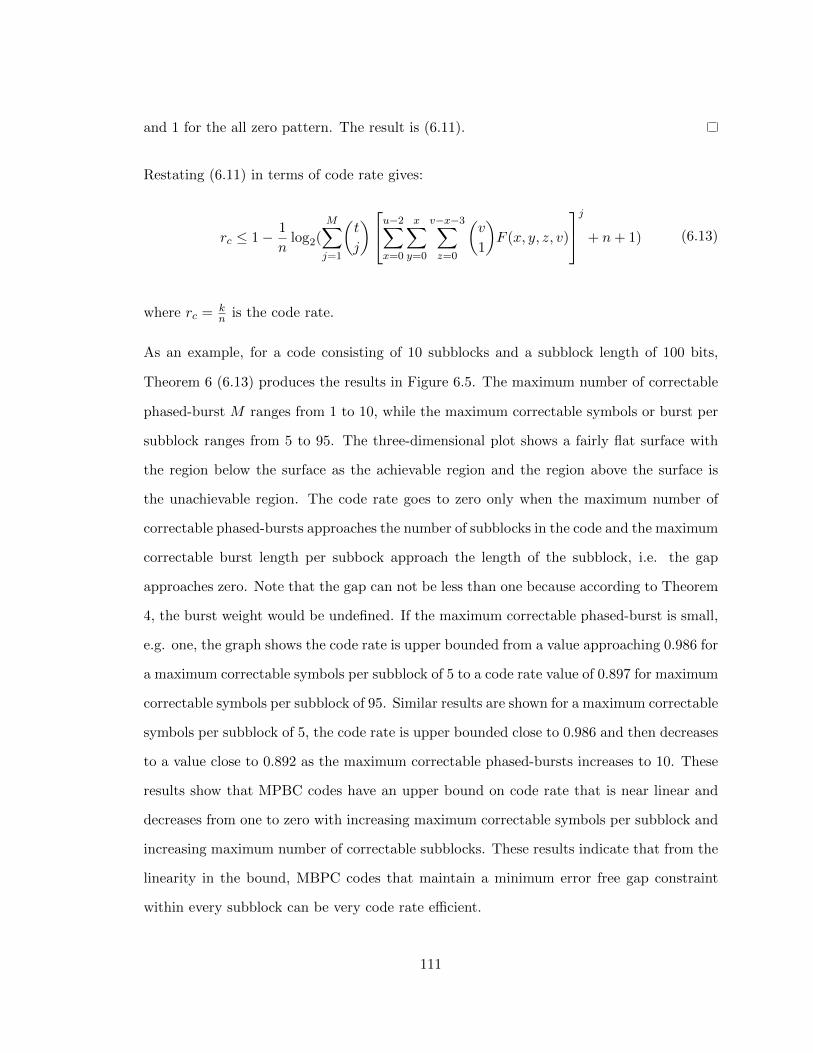
and 1 for the all zero pattern. The result is (6.11).

Restating (6.11) in terms of code rate gives:

rc ≤ 1− 1

nlog2(

M∑j=1

(t

j

)u−2∑x=0

x∑y=0

v−x−3∑z=0

(v

1

)F (x, y, z, v)

j + n+ 1) (6.13)

where rc = kn is the code rate.

As an example, for a code consisting of 10 subblocks and a subblock length of 100 bits,

Theorem 6 (6.13) produces the results in Figure 6.5. The maximum number of correctable

phased-burst M ranges from 1 to 10, while the maximum correctable symbols or burst per

subblock ranges from 5 to 95. The three-dimensional plot shows a fairly flat surface with

the region below the surface as the achievable region and the region above the surface is

the unachievable region. The code rate goes to zero only when the maximum number of

correctable phased-bursts approaches the number of subblocks in the code and the maximum

correctable burst length per subbock approach the length of the subblock, i.e. the gap

approaches zero. Note that the gap can not be less than one because according to Theorem

4, the burst weight would be undefined. If the maximum correctable phased-burst is small,

e.g. one, the graph shows the code rate is upper bounded from a value approaching 0.986 for

a maximum correctable symbols per subblock of 5 to a code rate value of 0.897 for maximum

correctable symbols per subblock of 95. Similar results are shown for a maximum correctable

symbols per subblock of 5, the code rate is upper bounded close to 0.986 and then decreases

to a value close to 0.892 as the maximum correctable phased-bursts increases to 10. These

results show that MPBC codes have an upper bound on code rate that is near linear and

decreases from one to zero with increasing maximum correctable symbols per subblock and

increasing maximum number of correctable subblocks. These results indicate that from the

linearity in the bound, MBPC codes that maintain a minimum error free gap constraint

within every subblock can be very code rate efficient.

111

Figure 6.5: MPBC Bound with a gap restriction for a Codelength of 10 Subblocks and 100bits per Subblock

Having explored the case of a coding bound where the phased-burst errors occur within

subblocks with a minimum error free gap specification, the case without a gap constraint is

addressed. In this instance, the MBPC codes are limited by a specified maximum number of

correctable symbols per subblock and the maximum number of correctable subblocks. This

bound is used to compare the impact to the code rate when the error free gap constraint is

observed. A special case of the bound where the maximum number of correctable symbols

per subblock equals to the length of the subblock is provided. For the first class of MPBC

superposition codes defined in the preceding sections, this special case is more applicable

since the error correction capability is over the entire subblock.

Theorem 7. The number of coset leaders, 2n−k, of a multiple phase correction linear block

code of length n = vt and dimension k, where v is the length of each subblock, t is number of

subblocks in a codeword, M is maximum number of correctable subblocks with a maximum

112

number of correctable symbols per subblock E is bounded by:

2n−k ≥M∑j=1

(t

j

)[ E∑l=1

(v

l

)]j+ 1. (6.14)

Proof. The proof is straightforward. Using similar arguments as the previous theorem, the

number of ways to correct l symbol errors in a subblock of length v is(vl

). For a maximum

number of E symbol errors in a subblock, a partial sum of these binomial coefficients is

taken where 1 ≤ l ≤ E or∑E

l=1

(vl

). If there are j correctable subblocks, then this result

needs to be raised to the jth power since the patterns in each subblock are disjoint. If

the largest number of subblocks that need to be corrected is M , then this calculation is

multiplied by the number of possible combinations(tj

)for every number j of correctable

subblocks, i.e. 1 ≤ j ≤ M and summed. Finally, a 1 is added to the total to included the

all zero codeword.

Equation (6.14) can be restated as

rc ≤ 1−log2(

∑Mj=1

(tj

) [∑El=1

(vl

)]j+ 1)

n(6.15)

where rc = kn is the code rate.

Figure 6.6 shows Theorem 7 (6.15) under the same code conditions as the example in Figure

6.5. To reiterate, this is a code consisting of 10 subblocks and a subblock length of 100

bits. The results show a concave surface as opposed the flat the surface of Figure 6.5. The

maximum number of correctable phased-bursts M ranges from 1 to 10, while the maximum

correctable symbols per subblock ranges from 5 to 95. The region below the surface is the

achievable region and the region above the curve is the unachievable region. If the maximum

correctable phased-burst is small, e.g. one, the graph shows the code rate is upper bounded

113

from a value 0.970 for a maximum correctable symbols/subblock of 5 bits to a code rate

value of 0.897 for a maximum correctable symbols/subblock of 95. Also, the code rate is

upper bounded close to 0.970 and then decreases to a value close to 0.738 as the maximum

correctable phased-bursts increases to 10. As in the previous result, the code rate goes to

zero only when the maximum number of correctable phased-bursts approaches the number

of subblocks in the code and the max correctable burst length per subbock approaches

the length of the subblock. However, unlike the previous results, the bound is much lower

in code rate. Also, note that for any given maximum correctable phased-burst value, the

region between 40 to 95 maximum correctable symbols/subblock is where the surface is the

steepest and very flat.

Figure 6.6: MPBC without a gap restriction for a Codelength of 10 Subblocks and 100 bitsper Subblock

To show the differences between the two bounds, a plot of them together is shown in Figure

114

6.7. The gap-restricted bound (6.13) is plotted on top while the bound without the gap-

restriction (6.15) is below. The maximum number of correctable phased-burst M ranges

from 1 to 10, while the maximum correctable symbols/subblock, u in (6.13) and E in

(6.15), ranges from 5 to 95. This shows that the gap-restricted upper bound is higher in

code rate than the upper bound without the gap restriction. The difference between the two

surfaces increases as the maximum correctable phased-burst increases. For a fixed value of

maximum correctable phased-burst, the difference between the two bounds will be nearly

zero while approaching 0 and 100 maximum correctable symbols/subblock. The difference

will increase as the maximum correctable symbols/subblock tends toward mid-range values.

This difference is largest at maximum correctable symbol/subblock of 34 for a particular

maximum number of correctable phased-bursts M . The largest difference in code rate is

0.502 occurring at the M = 10 and maximum correctable symbol/subblock of 34.

Figure 6.7: MPBC Bounds with and without a gap restriction

115

These bounds can now be used to measure the code rate efficiency of the examples given

in Section 6.4 for the first class of superposition code construction described in previous

sections. As mentioned before, these cases are where the entire subblock are correctable,

i.e. E = v. In this regard, the right side of (6.14) is reduced to:

2n−k ≥M∑j=1

(t

j

)(2v − 1)j + 1. (6.16)

The example code, studied in Figure 6.7, consisted of 10 subblocks and a subblock length

of 100 bits. The two bounds would approach the same value as the maximum correctable

symbols/subblock approach the length of the subblock. This should hold for the examples in

Section 6.4. That is since E = v, there is no gap restriction and burst errors are corrected

to the entire subblock length. Therefore, (6.15) and (6.13) (with gap set to its smallest

possible number, i.e. g = v − u = 1) will approach the same result (6.16).

For Example 1 of Section 6.4, the (4340, 3485) QC LDPC code with code rate approximately

0.803 is a multiple phased-burst error correction code capable of correcting a maximum of

M = 2 phased-bursts with a subblock length of v = 31 and t = 20. The bound given

by (6.13) predicts a code rate rc < 0.984 and (6.15) predicts a code rate rc < 0.984 also.

This shows a difference of 0.181 in code rate. While in Example 2 of Section 6.4, the

(37800, 34035) QC LDPC code with code rate approximately 0.900 is a multiple phased-

burst error correction code capable of correcting a maximum of M = 2 phased-bursts with

a subblock length of v = 63 and t = 40. Equation (6.13) predicts a code rate rc < 0.996 and

(6.15) predicts a code rate rc < 0.996 also. This shows a difference of 0.096 in code rate.

In both cases, (6.15), as expected, gives slightly lower values in code rate but the rounding

of (6.13) to three significant figures give approximately the same values to (6.15). That is,

(6.13) will always give a higher upper bound in code rate because of the gap restriction,

but when the gap is set to it’s smallest value of 1, the difference between (6.13) and (6.15)

when E = v, is very small.

116

In summary, Examples 1 and 2 of Section 6.4 show that the bounds (6.13) and (6.15) are

tight for this class of MPBC codes with Example 2 having an impressive 0.096 difference

between the code rate and bounds. In the next section, as a special case, this bound is

shown to be a generalization of a previously published single burst correction bound.

6.6 Single Burst Correction Bound

Up to this point, the first class of superposition MPBC codes have been defined and ana-

lyzed. Also, two MPBC bounds to measure how code rate efficient this class of codes are

have been presented. In this section, these bounds are analyzed under at a special case of

M = 1 which is an upper bound on the code rate of an SBC code. To do this, Theorem 6

is reduced to this corollary:

Corollary 2. A single burst correction code with block code of length n, dimension k and

maximum correction burst length u has the minimum number of coset leaders 2n−k bounded

by:

2n−k ≥(n

1

) u−2∑x=0

x∑y=0

n−x−3∑z=0

F (x, y, z, n) + n+ 1. (6.17)

Proof. A general linear block code can be considered an M = 1 multiple phase correcting

linear block code of length n since there is one subblock t = 1 that spans the entire code-

length, i.e. n = vt = v. This linear block code has dimension k and the maximum length of

a correctable phased-burst u where g = n−u is the error-free gap and therefore by applying

Theorem 6, results in (6.17).

Rewriting (6.17) in terms of code rate rc gives:

rc ≤ 1−log2(

(n1

)∑u−2x=0

∑xy=0

∑n−x−3z=0 F (x, y, z, n) + n+ 1)

n. (6.18)

117

Corollary 2 in the form of (6.18) gives an SBC upper bound on code rate that is not

constrained to the CBC. To explore the possible connections with previously published

bounds, the following corollary is proven:

Corollary 3. For a burst error pattern of length n whose burst length x+ 2 is constrained

under the CBC, the double summation of F (x, y, z, n) over variables 0 ≤ y ≤ x and 0 ≤

z ≤ x is equal to all possible binary vectors of length x, i.e.:

x∑y=0

x∑z=0

F (x, y, z, n) = 2x. (6.19)

Proof. Theorem 6 defines F (x, y, z, n) as a function that counts all patterns of length x

with the largest zero sequence of length z and the number of ones y. This includes the

all-zero pattern since by Theorem 4 the minimum burst weight is 2 for bursts that conform

to the CBC, i.e. these are two non-zero symbols that bound the all-zero pattern of length

x. Therefore, in (6.17), the maximum zero string parameter z is upper limited by x which

is the case when the when all-zero pattern occurs within a pattern of length x. Therefore,

by summing over all possible z and y which 0 ≤ y ≤ x and 0 ≤ z ≤ x, the result must equal

2x.

Corollary 3 can be used to evaluate (6.17) under the CBC condition. Then (6.17) be-

comes:

2n−k ≥(n

1

) u−2∑x=0

x∑y=0

x∑z=0

F (x, y, z, n) + n+ 1. (6.20)

That leads to:

2n−k ≥ nu−2∑x=0

2x + n+ 1. (6.21)

Recognizing that the summation is a geometric series that will equal to 2u−1 − 1, (6.21)

118

becomes

2n−k ≥ n(2u−1 − 1) + n+ 1 = n2u−1 + 1. (6.22)

Under the CBC condition, equation (6.22) is precisely the Hamming bound for burst-error

correction and when (6.22) is written in terms of required parity bits n − k becomes the

Abramson bound [12, p. 202]. Therefore, under the CBC condition, i.e. u ≤ bn+12 c, (6.17) is

the Abramson bound. And thus, (6.17) is a generalization of the Abramson bound without

the CBC restriction on the burst length.

At this point, the first class of MPBC codes has been presented and its performance in

AWGN and MPBC channels have been demonstrated. Two MPBC bounds have been

developed, in which one bound under special case of SBC was proved to be a generalization

of the Abramson bound. These bounds are used to show that the MPBC superposition

codes are very code rate efficient. A second class of superposition LDPC codes is now

presented.

119

Chapter 7: Multiple Burst Erasures Correction Coding

We now propose a class of MPBC LDPC product codes using the RED algorithm. A single

burst erasure correction algorithm was studied in [55, 56] for cyclic codes and [57, 58] for

any linear code for single burst erasure correction. We extend this technique exploiting the

structure of the parity-check matrix of product codes.

As a preliminary, from the Zero-Span Definition Section 4.2.3, we define the zero-covering

span as:

δ = minb

(maxiδFi,b). (7.1)

This quantity specifies the guaranteed single burst erasure correcting capability for a linear

block code using RED algorithm and is important in quantifying the burst erasure correction

capability of the LDPC product codes.

7.1 Product Codes for Erasure Correction

We introduced product codes in Section 3.4.2. In this section, we further expand the

definition. Recall that in Section 3.4.2, a two dimensional product code was defined as:

Definition 2. The generator matrix of a two-dimensional product code C1×C2, also denoted

CP , has a dimension k1k2 × n1n2 and is defined as:

GP = G2 ⊗G1 =

(G1g

(2)i,j

)(7.2)

where ⊗ is the Kronecker Product, and Gt =[g

(t)i,j

]is the generator matrix of component

code Ct of length nt, dimension kt, for t = 1 and 2.

120

If the order of C1 and C2 are switched, (7.2) becomes:

G∗P = G1 ⊗G2 =

(G2g

(1)i,j

). (7.3)

Note that GP and G∗P are combinatorially equivalent, i.e. they produce permuted versions

of each others codewords.

Product code encoding can often be described as an array structure as shown in Figure 7.1

[18, pp. 128-132]. The information sub-array contains the k1 × k2 information symbols to

be encoded. Each row of the information symbols is encoded according to the component

code generator matrix G1 and placed in the row of sub-array checks on rows. Then the

columns of the information symbols are encoded according to the component code generator

matrix G2 and placed in the columns of sub-array checks on columns. Finally, the checks

on checks sub-array is created either row-wise by encoding the checks on columns sub-array

rows according to G1 or column-wise by encoding the checks on rows sub-array according

to G2. The entire array is read out row by row and transmitted. However, if G1 and

G2 are switched in (7.3) as in the case of G∗P , the transmission is performed column by

column.

The parity-check matrix of a two dimensional product code can be defined as:

HP =

In2 ⊗H1

−−−−−

H2 ⊗ In1

(2n1n2−n1k2−n2k1)×n1n2

(7.4)

where H1 = {h(1)i,j }, i = (0, . . . ,m1−1), j = (0, . . . , n1−1); H2 = {h(2)

i,j }, i = (0, . . . ,m2−1),

j = (0, . . . , n2−1) are parity-check matrices of the component code C1, C2 respectively and

In1 , In2 are n1 × n1 and n2 × n2 identity matrices.

121

InformationChecks on

Rows

Checks on Columns

n1

k1

Checks on

Checks

k2

n2

Figure 7.1: Product Code Array

This is verified by noting that HP is the parity matrix of CP if and only if GPHTP = 0

then,

HTP =

In2 ⊗H1

−−−−−

H2 ⊗ In1

T

=

[(In2 ⊗H1)T |(H2 ⊗ In1)T

]

=

[In2 ⊗HT

1 |HT2 ⊗ In1

]n1n2×(2n1n2−n1k2−n2k1)

(7.5)

122

and,

GPHTP =

[G2 ⊗G1

] [In2 ⊗HT

1 |HT2 ⊗ In1

]

=

[[G2 ⊗G1

] [In2 ⊗HT

1

]]|[[

G2 ⊗G1

] [HT

2 ⊗ In1

]]

=

[[G2In2 ⊗G1H

T1

]|[G2H

T2 ⊗G1In1

]]

=

[[G2 ⊗ 0k1×(n1−k1)

]|[0k2×(n2−k2) ⊗G1

]]

= 0k1k2×(2n1n2−n1k2−n2k1).

(7.6)

A product code is a form of superposition construction. If H1 and H2 are LDPC matrices,

the Kronecker product used to form the product parity-check matrix HP in (7.5) is a

replacement method that can be viewed as a superposition of a base matrix In2 with a

single constituent matrix H1 for the In2 ⊗H1 submatrix and also a superposition of base

matrix H2 with a single constituent matrix In1 for the H2 ⊗ In1 submatrix. We note that

while the submatrix In2⊗H1 maintains the replacement constraint, the In1 for the In1⊗H2

submatrix in general does not. The exception being that if H2 is a permutation matrix then

the replacement constraint is maintained. However, we will prove later that if both H1 and

H2 conforms to the RCC then HP also conforms to the RCC.

123

7.1.1 Parity-Check Matrix Structure

Equation (7.4) defines the parity-check matrix of a two-dimensional product code that can

be partitioned into two submatices:

HP =

A1

−−

A2

=

H1 0 0 . . . 0

0 H1 0 . . . 0

0 0 H1 . . . 0

......

......

...

0 0 0 . . . H1

h(2)0,0In1 h

(2)0,1In1 h

(2)0,2In1 . . . h

(2)0,n2−1In1

h(2)1,0In1 h

(2)1,1In1 h

(2)1,2In1 . . . h

(2)1,n2−1In1

h(2)2,0In1 h

(2)2,1In1 h

(2)2,2In1 . . . h

(2)2,n2−1In1

......

......

...

h(2)m2−1,0In1 h

(2)m2−1,1In1 h

(2)m2−1,2In1 . . . h

(2)m2−1,n2−1In1

(7.7)

where m2 = n2 − k2,

A1 = In2 ⊗H1 =

H1 0 0 . . . 0

0 H1 0 . . . 0

0 0 H1 . . . 0

......

......

...

0 0 0 . . . H1

(7.8)

and

124

A2 = H2 ⊗ In1 =

h(2)0,0In1 h

(2)0,1In1 h

(2)0,2In1 . . . h

(2)0,n2−1In1

h(2)1,0In1 h

(2)1,1In1 h

(2)1,2In1 . . . h

(2)1,n2−1In1

h(2)2,0In1 h

(2)2,1In1 h

(2)2,2In1 . . . h

(2)2,n2−1In1

......

......

...

h(2)m2−1,0In1 h

(2)m2−1,1In1 h

(2)m2−1,2In1 . . . h

(2)m2−1,n2−1In1

. (7.9)

The ith row of A2 is:[h

(2)i,0 In1 h

(2)i,1 In1 h

(2)i,2 In1 . . . h

(2)i,n2−1In1

]. This can be expanded and

partitioned into a n1 × n1n2 submatrix:

h(2)i,0 0 . . . 0 h

(2)i,1 0 . . . 0 . . . h

(2)i,n2−1 0 . . . 0

0 h(2)i,0 . . . 0 0 h

(2)i,1 . . . 0 . . . 0 h

(2)i,n2−1 . . . 0

......

......

......

......

......

......

...

0 0 . . . h(2)i,0 0 0 . . . h

(2)i,1 . . . 0 0 . . . h

(2)i,n2−1

.

(7.10)

This is a submatrix where every row is right cyclic shift of its previous row within each

section.

We see that the parity-check matrix (7.7) has n2 column-phases of length n1. Then (7.8)

is a submatrix consisting of n2 row-phases of length m1 = n1 − k1 and (7.9) is a submatrix

consisting of m2 = n2 − k2 row-phases of length n1.

Under certain conditions, we can show that equation (7.7) has the RCC property.

125

7.2 Analysis of LDPC Product Codes

In this section, the degree distribution of HP is analyzed based on the degree distributions

of constituent codes. But first, HP is demonstrated to conform to the RCC.

Theorem 8. If H1 and H2 have the RCC property then HP also conforms to the RCC.

Proof. The RCC condition states that for any pair of row indices i1, i2 and any pair of

column indices j1, j2; hi1,j1 ,hi2,j1 , hi1,j2 , and hi2,j2 can not all be non-zero elements. From

the structure of A1, (7.8) shows that no two columns (rows) that are not within a column-

phase (row-phase) have co-incident non-zero elements. Since H1 adheres to the RCC, then

every column (row) within a column-phase (row-phase) adheres to RCC and therefore A1

adheres to the RCC. Matrix A2, (7.9), can be seen as a superposition with a base matrix

H2 that adheres to the RCC, with a set of n1× n1 constituent matrices {In1 ,On1×n1} that

are CPMs. Therefore, A2 conforms to the RCC. What’s left now is to show that A1 and A2

jointly adheres to the RCC. By the argument above that for A1, no two columns that are

not within a column-phase have co-incident non-zero elements, then all that is required is to

show is that the RCC is met within any column-phase in HP . Any row in a column-phase

of A2 has at most unit weight, since by construction, any column-phase of A2 is a column

array from the set {In1 ,On1×n1}. Therefore no pair of column indices have co-incident

non-zero elements for any one row from A2 and any other row from A1. Then the RCC is

adhered to within any column-phase of HP . Therefore, HP adheres to RCC.

Having established the condition for HP to meet the RCC, the goal is to explore the

implications of HP defining an LDPC code by calculating it’s degree distribution based on

component distributions of H1 and H2 with the next theorem. From this work, the goal is

then to predict the performance of HP from the characteristics of the components.

Theorem 9. Let the degree polynomial pairs of the component codes C1 and C2 be (τ (1)(x), ρ(1)(x))

and (τ (2)(x), ρ(2)(x)) respectively, with τ(1)i , ρ

(1)i and τ

(2)i , ρ

(2)i , degree distributions respec-

tively (as defined in Section 3), then the degree polynomial pair of the LDPC Product code

126

using HP is

(τP (x), ρP (x)) = (τ (1)(x)τ (2)(x)x, d1ρ(1)(x) + d2ρ

(2)(x))

where d1 = m1n2m1n2+m2n1

, d2 = m2n1m1n2+m2n1

, m1 = n1 − k1 and m2 = n2 − k2.

Proof. τP (x) and ρP (x) are proved separately. First, from (7.7) the lth column-phase of

HP has a contribution from A1 and A2. The VN degree polynomial τ (1)(x) applies to every

column-phase in A1. The lth column-phase of A2 is a constant degree distribution of the

lth bit of H2. Therefore the lth column-phase of (7.7) can be written as: τ (1)(x)xv where

v is the column degree of H2 at column l. The fraction of column-phases of HP with this

degree distribution is τ(2)v , therefore the fraction of column-phases with degree polynomial

τ (1)(x)xv is τ(2)v τ (1)(x)xv. By summing all fractions of column-phases of degree polynomial

τ (1)(x)xv for all possible v, the total variable degree polynomial is

τP (x) =∑v

τ (2)v τ (1)(x)xv =

∑v

∑i

τ (2)v τ

(1)i xi−1xv−1x = τ (1)(x)τ (2)(x)x.

Since, HP is a vertical stacking of A1 and A2, ρP (x) is the apportioned sum of row degree

polynomials from A1 and A2, i.e. ρ(1)(x) and ρ(2)(x), respectively. The number of rows in

A1 and A2 is m1n2 and m2n1 therefore ρP (x) = d1ρ(1)(x) + d2ρ

(2)(x).

This theorem shows that VN degree polynomial of the product code is a direct polynomial

multiplication of the VN degree polynomials of the component codes. This bound can be

used on the minimum distance of the product LDPC code. By calculating the minimum

weight of the columns of HP , the minimum distance of an LDPC code is bounded by

dmin ≥ γ + 1, where γ is the column weight of a regular LDPC code.

The following observations are the direct result of Theorem 9 noting that if γmin1 and γmin2

are the smallest degree terms in τ (1)(x) and τ (1)(x) respectively, then the smallest degree

term in τP (x) is τγmin1τγmin2xγmin1+γmin2−1. From this result, the following three corollaries

127

are developed.

Corollary 4. If H1 and H2 are parity-check matrices of regular LDPC codes with column

weights γ1 and γ2 respectively, then HP is the parity-check matrix of a regular LDPC code

of column weight γP = γ1 + γ2.

Corollary 5. If H1 and H2 are parity-check matrices of irregular LDPC codes of minimum

column weights γmin1 and γmin2 respectively, then HP is the parity-check matrix of an

irregular LDPC code whose minimum column weight is γminP = γmin1 + γmin2.

Corollary 6. If HIRR and HREG are the parity-check matrices of irregular and regular

LDPC codes of minimum column weight γminIRR and column weight γREG respectively,

where either codes can be component codes H1 or H2 of a product code then HP is parity-

check matrix of an irregular LDPC code of minimum column weight γminP = γminIRR +

γREG.

Corollaries 4 and 5 were first proved in [63].

As stated before, the minimum distance of a regular LDPC code of column weight γ is

at least γ + 1. From Corrolary 4, it is apparent that this bound is rather weak, i.e. if

the minimum distance of the component codes C1 and C2 are dmin1 and dmin2 respectively,

then the minimum distance of the product code is dminP = dmin1dmin2. However, applying

Corollary 4 gives

dminP ≥ γ1 + γ2 + 1. (7.11)

7.2.1 Multiple Burst Erasure Correcting Capability

To this point, the second class of superposition LDPC codes has been defined and analysis

on the parity-check matrix has been performed, i.e. its proven to conform with the RCC and

its degree distribution calculated. The goal now is to investigate the multiple phased-burst

erasure correcting capability of this class of codes.

Note that A2 is a matrix whose construction can be described as that in Section 6.2.

Therefore Theorem 2 says the product code CP can be decoded using OSMLD on A2 only

128

and thus can correct bγ2/2c MPEr bursts of length n2. Even though this decoding is

possible, it completely ignores the contribution from A1. This can be improved by using

a recursive erasure decoder which is describe below. To find the multiple burst erasure

correcting capability of a product code using a recursive erasure decoder, the following

lemma is proved.

Lemma 1. The Kronecker product of H2⊗In1, where In1 is an identity matrix of dimension

n1×n1 and H2 is an m2×n2 matrix with a zero-covering span of δ2, produces an n1m2×n1n2

matrix that has a zero-covering span of δ = n1(δ2 + 1)− 1.

Proof. The zero-spans in (7.10) are defined by the non-zero elements of h(2)i,j where 0 ≤

i < m2 and 0 ≤ j < n2. That is for every [b, e]i ordered pair of column indices of the ith

row in H2 where b, e ∈ {0, 1, . . . , n2 − 1}, there is an associated set of n1 ordered pairs,

{[B,E]i}, of non-zero element column positions in (7.10) where B = bn1 + u, E = en1 + u

and B,E ∈ {0, 1, . . . , n1n2 − 1} with 0 ≤ u < n1 as the relative row index offset of the ith

submatrix. Therefore, (7.10) has forward zero-spans that are of length:

δFi,B = (E −B)n1n2 − 1 = ((e− b)n1)n1n2 − 1

= ((e− b)n2)n1 − 1 = (δFi,b + 1)n1 − 1.

(7.12)

To find the zero-covering span, a minimization over all B of the maximum of (7.12) over all

i (submatrices of (7.9)) gives:

δ = minB

(maxiδFi,B) = min

B(max

i(δFi,b + 1)n1 − 1)

= minb

(δFb + 1)n1 − 1 = (δ2 + 1)n1 − 1.

(7.13)

The final step in (7.13) comes is the recognition that a minimization over B is a minimization

over b since (7.12) says that δFi,B is only dependent on b.

129

The prior theorem is used to find the erasure correcting capability of HP with the following

theorem.

Theorem 10. A two dimensional product code, CP , with component codes C1(n1, k1),

C2(n2, k2) with zero-covering spans of δ1 and δ2 respectively, can correct a single burst of

size bA2 = n1(δ2 + 1) or multiple erasure bursts of size bA1 = n2 × (δ1 + 1) using the RED

algorithm.

Proof. Equation (7.7) defines the parity-check matrix of a two-dimensional product code

which can be partitioned into two submatrices where A1 and A2 are defined in (7.8) and

(7.9) respectively. If H1 has a zero-covering span of δ1 and A1 acts on n2 codewords of C1,

then A1 can correct multiple erasure burst confined in each codeword of up to b1 = δ1 + 1

symbols or

bA1 = n2 × (δ1 + 1) (7.14)

symbols.

A2 is formed by replacing every non-zero element of H2 by an In1 identity matrix which has

a zero-span of n1 − 1 and every zero element of H2 is replaced by an all zero n1×n1 matrix,

0n1×n1 , which has a zero-covering span of n1. Lemma 1 says that a Kronecker product of

H2 ⊗ In1 results in an overall zero-covering span of n1(δ2 + 1) − 1. Therefore, if H2 has a

zero-covering span of δ2 then A2 has a zero-covering span of δA2 = n1δ2 + n1 − 1 and can

correct any erasure burst up to length,

bA2 = δA2 + 1 = n1(δ2 + 1).

Theorem 10 can be interpreted to say that the guaranteed largest number of erasures that

the product code can correct using a recursive erasure decoder is bA1 or bA2 . To achieve

this performance, an additional requirement while using A1 to decode is that the erasure

130

bursts need to be separated by a guard band of n1 − δ1 − 1.

7.3 Decoding Algorithms

To document a possible decoding algorithm, some terminology must be defined. A con-

strained burst in submatrix A1 is defined as an erasure burst that is within the erasure

correcting capability δt + 1 of the tth component code where t ∈ {1, 2}. That is, within the

boundary of a component codeword, there is at least nt− δt− 1 consecutive bits (including

end around) with no erasures. For instance, in (7.8) there are n2 component codewords

from H1 of length n1 bits where each component codeword can correct δ1 + 1 erased bits

and must contain a string of at least n1 − δ1 − 1 consecutive bits with no erasures.

7.4 Product Code Multiple Burst Erasure Decoding Algo-

rithm

1. Determine if received codeword has any erasures. If none, then output received code-

word.

2. Else, if the erasures can be characterized as n2 constrained bursts of length δ1 +1 bits,

use submatrix A1 with RED (see Section 4.2.2) to correct all bits. Output corrected

codeword and stop.

3. Else, if residual erasures are present and if the erasures that can be characterized as a

burst of length n1(δ2 +1), use submatrix A2 with the RED to correct all bits. Output

corrected codeword and stop.

4. Else, interleave codeword by switching G1 and G2 position in (7.2) to (7.3) thus

A1 ⇒ In1 ⊗H2 and A2 ⇒ H1 ⊗ In2 . If the residual erasures can be characterized as

n1 constrained bursts of length δ2 + 1 bits, use submatrix A1 with RED to correct all

131

bits. Output corrected codeword and stop.

5. If the residual erasures that can be characterized as a burst of length n2(δ1 + 1) use

submatrix A2 with the RED to correct all bits. Output corrected codeword and stop.

6. Otherwise, declare decoder failure and stop.

7.4.1 Examples of LDPC Product Codes for Burst Erasure Correction

In this section, we give two examples to show that the effectiveness of LDPC product codes

for correcting erasure bursts. The two examples are based on three component codes: 1) a

(63, 37) LDPC code based on lines of Euclidean geometry, EG(2, 23) over GF(23) [18, pp.

860-866], with rate rc = 0.587 with a zero-covering span δ = 23, minimum distance dmin = 9,

column weight γ = 8 and denoted as EG(63, 37); 2) a (255, 175) LDPC code based on lines of

Euclidean geometry, EG(2, 24) over GF(24) [18, pp. 860-866], with a code rate rc = 0.686,

a zero-covering span δ = 55, minimum distance dmin = 17, column weight γ = 16 and

denoted as EG(255, 175); and 3) a code rate rc = 0.984 (63, 62) single parity-check code

(SPC) with a zero-covering span δ = 0. The (63, 62) SPC code consists of a single row of 63

non-zeros for the parity-check matrix. Although it is not strictly an LDPC code since there

are only non-zero entries, it does not have any cycles but does have a low minimum distance

of 2. The SPC code was selected as a second component code to the EG(255,175) code to

keep the product code rate as high as possible while keeping the overall length of the code

around 16K bits. This is considered a medium to large block size in the literature.

Example 1. Consider the product code EG(63,37)×EG(63,37). According to Theorem

10, this (3969, 1369) LDPC product code with rate 0.3449 can correct a large erasure burst

totaling bA2 = 63(23 + 1) = 1, 512 bits or bA1 = 63 multiple bursts of length 24 bits.

Equation (7.11) estimates the minimum distance to be dmin ≥ 2(8) + 1 = 17 but its true

minimum distance is dmin = 92 = 49, so this estimate is loose in this case. In addition,

we have thus far only considered erasure burst correction, however Theorem 8 says that

132

the product code parity-check matrix HP is an LDPC code as well. Therefore, we now

demonstrate that this LDPC product code also has good performance over the BEC using

the LDPC erasure decoding algorithm defined in [52]. For this example, the bit erasure

rate (BER) and frame erasure rate (FER) performance over the binary erasure channel is

plotted in Figure 7.2. Notice that the performance differs from the channel capacity by

0.135 in erasure probability rate ε at a BER of 1.629e− 06 and FER of 3.441e− 06. These

are excellent results for a small block length code.

Erasure Probability ǫ0 0.1 0.2 0.3 0.4 0.5 0.6 0.7 0.8 0.9 1

BE

R/F

ER

10-6

10-5

10-4

10-3

10-2

10-1

100

Binary Erasure Channel Performance of (3969,1369) Rate=0.3449EG(63,37)xEG(63,37) Product Code

BERFERChannel Capacity

Figure 7.2: BEC Performance of EG(63,37)×EG(63,37)

Example 2. Consider the product code SPC(63,62)×EG(255,175). This (16065, 10850)

LDPC product code with rate 0.6754 can correct a large erasure burst totaling bA2 =

255(0 + 1) = 255 bits or bA1 = 63 multiple bursts of length 56 bits according to Theorem

10. Equation (7.11) estimates the minimum distance to be dmin ≥ 16 + 1 + 1 = 18 but its

true minimum distance is dmin = 17(2) = 34, so this estimate is tighter than Example 1 but

still loose. In addition, we have thus far only considered erasure burst correction, however

133

Theorem 8 says that the product code parity-check matrix HP is an LDPC code as well.

Therefore, we now demonstrate that this LDPC product code also has good performance

over the BEC using the LDPC erasure decoding algorithm defined in [52]. Its bit erasure

rate (BER) and frame erasure rate (FER) performance is plotted in Figure 7.3. Its BER

performance of 2.4690e− 7 and FER performance of 4.4663e− 6 is within 0.0846 in erasure

probability rate of the channel capacity. Again, these are excellent results for a medium

size block.

Erasure Probability ǫ

0 0.1 0.2 0.3 0.4 0.5 0.6 0.7 0.8 0.9 1

BE

R/F

ER

10-7

10-6

10-5

10-4

10-3

10-2

10-1

100

Binary Erasure Channel Performance of (16065,10850) Rate=0.6754

SPC(63,62)xEG(255,175) Product Code

BER

FER

Channel Capacity

Figure 7.3: BEC Performance of SPC(63,62)×EG(255,175)

Having explored the burst erasure correcting capability of HP , the focus is now on the

AWGN channel. Theorem 8 says that if H1 and H2 are parity-check matrices of LDPC

codes, then HP will be the parity-check matrix of an LDPC code and therefore the use of

the SPA over the AWGN channel can be explored in the next section.

134

7.5 Product Code LDPC Decoding Algorithm for AWGN

While the above exposition focused primarily on the burst channels, the goal is to develop

codes that can operate well in both burst and random channels, i.e., AWGN. This algorithm

is also useful, in case there are a small number of residual errors that occur after the

product code multiple burst erasure decoding algorithm described in Section 7.4. Theorem

8 shows that HP can be used directly in a SPA decoder. However, HP has a number of

redundant rows. The number of independent rows for any parity-check matrix of CP should

be n1n2−k1k2 but the number of rows in HP is mP = 2n1n2−n1k2−n2k1. The difference of

these values shows that the number of redundant rows is (n1−k1)(n2−k2). From Section 7.1,

this is precisely the number of checks on checks. This redundancy gives the structure of HP .

There is the option to puncture the checks on checks bits. If choosen to do so, the minimum

distance of this incomplete product code will be reduced to dminP = dmin1 + dmin2 − 1,

however the code rate will improve. A possibly more efficient decoder is the following.

7.5.1 Two-Stage LDPC Product Code Decoder

A product code decoder for the AWGN channel can be developed based on the following

concept. Use component LDPC SPA decoders that will be coordinated such that APP infor-

mation estimates at the output of one component LDPC SPA decoder will be interleaved

and used as priors to the other component LDPC SPA decoder. A complete processing

of both decoders form a full decoding iteration. Perform multiple iterations until the de-

coder finds a codeword or until a maximum iteration has been achieved. By doing so, the

LDPC product codes require much less resources, since the codeword is composed of multi-

ple smaller codewords that can be decoded with one single implementation. Therefore the

complexity is reduced by a fraction of the total code length. A block diagram for a two

component product LDPC SPA decoder is shown in Figure 7.4. The C1 decoder accepts, as

priors, LLR channel inputs (defined in Section 3.5) and produces an estimate APP measure

after one (or more) complete C1 component decode. Then the APP measure is re-ordered

135

so that C2 codewords are formed sequentially. The C2 decoder accepts the re-ordered APP

measure and produces an updated APP measure based on one (or more) complete C2 com-

ponent decode. This update gets re-ordered back to the original form, i.e. sequential C1

codewords. Then a syndrome calculation based on Cp is performed to check for a valid code-

word or if a maximum number of iterations has been reached. If this condition has occurred

then output the estimated codeword, else start (or iterate) the process over again with the

re-ordered updated APP measures from C2 decoder as priors to the C1 decoder.

Channel Inputs

C1 LDPC SPA Decoder

Interleaver

C2 LDPC SPA Decoder

De-Interleaver

Estimated Codeword

Figure 7.4: Two-Stage LDPC Product Code Decoder

Having analyzed the burst erasure correcting capability and showed that product codes

136

with constituent LDPC codes meet the RCC, novel decoders for correcting burst erasures

and for the AWGN channel are presented. In the next section, examples of this class of

codes with simulations and analyses are discussed.

7.6 Product LDPC Code Examples and Results

Simulations in AWGN were performed with 3 types of component linear block codes: 1)

a code rate rc = 0.686 Euclidean Geometry C(1)EG(2, 0, 4) (255, 175) LDPC code [18, pp.

860-866] with a zero-covering span δ = 55, 2) a code rate rc = 0.686 PEG (255, 175)

LDPC code of column weight 4 [65] with a zero-covering span δ = 28, and 3) a code rate

rc = 0.984 (64, 63) single parity-check code (SPC) [18, pp. 94-95] with a zero-covering span

δ = 0. The (64, 63) SPC code consists of a single row of 64 ones for the parity-check matrix.

Although it is not strictly an LDPC code since there are only non-zero components, it

does not have any cycles but does have a low minimum distance of 2. The SPC code was

selected as a second component code to the EG or PEG code to keep the product code rate

as high as possible while keeping the overall length of the code around 16K bits. This is

considered a medium to large block size in the literature and would help keep simulation time

manageable. The maximum number of iterations was set to 50 for component EG decoding

and 50 for component PEG decoding, with the overall maximum number of iterations for

product code decoding set to 50.

First, the EG and PEG codes by themselves are simulated with the SPA to establish a

performance baseline. Figure 7.5 is a plot of the bit error rate (BER) and the block error

rate (BLER) of the EG (255, 175) code. Figure 7.6 is a plot of the BER and BLER for

the PEG (255, 175) code. The EG code is the better performing code in terms of BER and

BLER with about a 0.8 dB improvement at 1e-6 BER.

These codes are now used in the product LDPC decoder as described above. Figure 7.7

shows the PEG code when used as a (65025, 30625) product LDPC code at a product code

137

3 4 5 6 7 8 9 10 1110−7

10−6

10−5

10−4

10−3

10−2

10−1

Eb/No

Err

or R

ate

EG (255,175) SPA Performance with 50 Iterations

BERBLERTheoretical BPSK

Figure 7.5: EG (255,175) LDPC Code with SPA in AWGN Channel

3 4 5 6 7 8 9 10 1110 8

10 7

10 6

10 5

10 4

10 3

10 2

10 1

Eb/No

Err

or R

ate

PEG (255,175) LDPC Regular Degree 4 with SPA @ 200 Max Iter

BERBLERBPSK

Figure 7.6: PEG (255,175) Code with SPA in AWGN Channel

138

rate of rc = 0.471. The results indicate that product decoder has 1.2 dB improvement at

1e-6 BER over the PEG code alone while incurring a rate loss using the product code. There

is also a significant error floor that starts at 3.5 dB. The EG (255,175) code, on the other

hand, makes a better argument for the product code. The simulations indicate, see Figure

7.8, that the (65025, 30625) EG product code of rate rc = 0.471 can provide near-error free

performance after 3.4 dB while the slope of the baseline EG code alone is lower and will

need more signal power to achieve the same error rate. Also, comparing the EG product

code versus the PEG product code, the EG product code is superior at ≥ 3.4 dB.

3 4 5 6 7 8 9 10 1110 8

10 7

10 6

10 5

10 4

10 3

10 2

10 1

100

Eb/No

Err

or R

ate

PEG (255,175)×PEG (255,175) Error Performance

PEG BERPEG BLERTheoretical BPSKPEGxPEG BERPEGxPEG BLER

Figure 7.7: PEG (255,175)×PEG (255,175) in AWGN Channel

Figures 7.9 and 7.10 show the PEG×SPC rate rc = 0.676 (16320, 11025) product code and

the EG×SPC rate rc = 0.676 (16320, 11025) product code, respectively. The PEG×SPC

product code performs marginally better than the PEG code alone and worse than the

PEG×PEG product code at 1e-6 BER with a noticeable crossover at around 2e-7 BER.

The EG×SPC product performs slightly better than the EG (255, 175) alone with a small

139

3 3.2 3.4 3.6 3.8 4 4.2 4.4 4.6 4.8 510−7

10−6

10−5

10−4

10−3

10−2

10−1

100

Eb/No

Err

or R

ate

EG(255,175) vs. EG(255,175) × EG(255,175) Error Performance with 50 Iterations

EG(255,175) BEREG(255,175) BLEREG(255,175) × EG(255,175) BEREG(255,175) × EG(255,175) BLERTheoretical BPSK

Figure 7.8: EG (255,175)×EG (255,175) in AWGN Channel

rate loss and small hardware penalty for the additional SPC decoder.

According to Theorem 10, any code can improve its burst correction performance and

correct multiple bursts by its use in a product code. That is, a product code has the erasure

correction capability of a single burst of size bA2 = n1(δ2 + 1) or a multiple erasure burst

correcting capability of bA1 = n2×(δ1+1). For the PEG codes where δ = 28, the PEG×PEG

product code can correct a large erasure burst totaling bA2 = 255(28 + 1) = 7, 395 bits or

bA1 = 255 multiple bursts of length 29 bits and PEG×SPC product code can correct one

large burst of bA2 = 255(0+1) = 255 bits or bA1 = 64 multiple bursts of length (28+1) = 29

bits. For the EG codes where δ = 55, the EG×EG product code can correct a large erasure

burst totaling bA2 = 255(55 + 1) = 14, 288 bits or bA1 = 255 multiple bursts of length 56

bits and EG×SPC product code can correct one large burst of bA2 = 255(0 + 1) = 255 bits

or bA1 = 64 multiple bursts of length (55 + 1) = 56 bits. This is even more rationale for

using either the EG×EG product or the EG×SPC product. Not only do the EG product

codes show good AWGN performance, but they perform very well for multiple phased-

burst erasure correction and their overall performance are better than the PEG product

140

3 4 5 6 7 8 9 10 1110 8

10 7

10 6

10 5

10 4

10 3

10 2

10 1

100

Eb/No

Err

or R

ate

PEG (255,175)×SPC (64,63) Error Performance

PEG BERPEG BLERTheoretical BPSKPEGxSPC BERPEGxSPC BLER

Figure 7.9: PEG (255,175)×SPC (64,63) in AWGN Channel

3 3.2 3.4 3.6 3.8 4 4.2 4.4 4.6 4.8 510−8

10−7

10−6

10−5

10−4

10−3

10−2

10−1

100

Eb/No

Err

or R

ate

EG(255,175) vs. EG(255,175) × SPC(64,63) Error Performance

EG BEREG BLEREG × SPC BEREG × SPC BLERTheoretical BPSK

Figure 7.10: EG (255,175)×SPC (64,63) in AWGN Channel

141

codes.

142

Chapter 8: Conclusion

In Chapters 4 and 5, we successfully analyzed the ensemble of randomly generated left

regular LDPC codes with parity-check matrices of constant column weights. We showed

that the mean for Zero-covering span profile δFl PMF does not change appreciably with

increasing block sizes. And these Zero-covering span profiles δFl can have much larger

means than their Correctible profiles γFl means. Moreover, the Correctible profile γFl under

the RED algorithm as well as the Zero-covering span profile δFl performance are a function

of column weight of the parity-check matrix. We also demonstrated that the mean for the

Correctible profile γFl does reduce with increasing block size. However, for the asymptotic

case as the block size grows to infinity, it is proved that these codes are good for burst

erasure correction. Additionally, these LDPC codes have very large average zero-covering

spans. This indicates that there might be other algorithms yet to be explored that can take

advantage of the large spans without the decoder failures presented by the RED algorithm.

One possibility is the use of the Forward-Backward Algorithm described in [57]. However

the forward-backward Correctible profile PMF is much harder to analyze. Furthermore,

we demonstrated that given a specific set of parameters, i.e. block length, parity-check

matrix density, and rate; and through random construction, it’s quite easy to design an

ensemble that will, on the average, correct a burst of a specific number of erasures using a

very low complexity decoder. And we showed that the analyses presented are very accurate

in predicting the average ensemble performance. In addition, the expurgated ensemble was

analyzed and it was found that it performs better than the unexpurgated ensemble. And

that the use of the expurgated ensemble is the recommended choice for code design.

In Chapters 6 and 7, we presented two methods for flexible algebraic constructions of

multiple phased-burst errors and erasures correcting superposition LDPC codes, which also

143

have good performances in the AWGN channels and erasure channels. It is shown that

in the first construction, the phased-burst erasures correcting capability is not only lower

bounded by column weights, but also lower bounded by stopping sets. Also, it is shown

that by using simple majority logic decoding, powerful MPBC coding can be designed.

We demonstrated how well these codes are constructed by comparing them to two lower

bounds constructed for MPBC coding, one based on a strict definition of a phase burst

with an error free gap and another without the gap distinction. In both cases, the codes

presented here are tight with these bounds and demonstrate that these are very efficient

in coding rate for MPBC correction. It is shown that the bound with the gap distinction

is a generalization of the Abramson bound for single burst correction. In addition, a novel

burst erasure decoder that exploits the zero-span characteristics of product LDPC codes

was presented. These codes can easily be designed to decode a large single erasure burst or

multiple smaller phased erasure bursts. It was demonstrated that product codes based on

constituent LDPC codes are also LDPC codes. Simulations were performed for two example

LDPC Product Codes over the BEC. The results indicate that the erasure performances

approach the channel capacity. A novel iterative SPA decoding based on component LDPC

decoders was developed and its performance was demonstrated.

Overall, this dissertation is proof that we were successful in achieving our goals of finding

novel approaches to solving the classical problem of burst erasure/error correction. We

based our search on LDPC codes and showed that LDPC can in fact lead to simple imple-

mentations for decoding, i.e. the RED algorithm, OSMLD and component SPAs; as well

as encoding, i.e. superposition with cyclic encoders and product encoding, while provid-

ing near theoretical performance with our bounds. We also showed that code design can

be accomplished simply with random construction or superposition construction and still

achieve excellent performance. Ultimately, we achieved our main goal of designing codes or

designing simple coding techniques that can correct a burst or average burst erasure/error

for specified length of a particular block size.

144

Bibliography

145

Bibliography

[1] W. H. Fong, Q. Huang, S.-C. Chang, and S. Lin, “Multiple phased-burst correctingsuperposition product LDPC codes,” in 2011 IEEE International Conference on Com-munications. ICC ’11. IEEE, June 2011, pp. 1–5.

[2] S. Johnson, “Burst erasure correcting LDPC codes,” IEEE Transactions on Commu-nications, vol. 57, no. 3, pp. 641–652, March 2009.

[3] E. Paolini and M. Chiani, “Construction of near-optimum burst erasure correcting low-density parity-check codes,” IEEE Transactions on Communications, vol. 57, no. 5, pp.1320–1328, May 2009.

[4] L. C. Andrews and R. L. Phillips, Laser Beam Propagation through Random Media.SPIE Press, 2005.

[5] Consultative Committee for Space Data Systems (CCSDS), “Implementationof a DVB-S2 Encoder and Decoder for the LCRD Mission.” [Online].Available: http://cwe.ccsds.org/sls/docs/SLS-CandS/Meeting%20Materials/2013/2013 04%20Bordeaux/SLS-CS 13-09-DVBS2 Implementation.pdf

[6] D. Bertsekas and R. Gallager, Data Networks. Prentice Hall, 1992.

[7] D. Tse and P. Viswanath, Fundamentals of Wireless Communication. CambridgeUniversity Press, 2005.

[8] S. B. Wicker and V. K. Bhargava, Reed-Solomon Codes and Their Applications. JohnWiley and Sons, 1999.

[9] J. P. Nguyen, “Applications of Reed-Solomon codes on optical media storage,” Ph.D.dissertation, San Diego State University, 2011.

[10] Consultative Committee for Space Data Systems (CCSDS), “TM Synchronizationand Channel Coding. Blue Book. Issue 2. August 2011.” [Online]. Available:http://public.ccsds.org/publications/archive/131x0b2ec1.pdf

[11] M. Cominetti and A. Morello, “Digital video broadcasting over satellite (DVB-S):a system for broadcasting and contribution applications,” International Journal ofSatellite Communications, vol. 18, no. 6, pp. 393–410, 2000.

[12] R. McEliece, The Theory of Information and Coding. Cambridge University Press,2002.

146

http://cwe.ccsds.org/sls/docs/SLS-CandS/Meeting%20Materials/2013/2013_04%20Bordeaux/SLS-CS_13-09-DVBS2_Implementation.pdf

http://cwe.ccsds.org/sls/docs/SLS-CandS/Meeting%20Materials/2013/2013_04%20Bordeaux/SLS-CS_13-09-DVBS2_Implementation.pdf

http://public.ccsds.org/publications/archive/131x0b2ec1.pdf

[13] C. E. Shannon, “A mathematical theory of communication,” Bell System TechnicalJournal, vol. 27, pp. 379–423 and 623–656, July and October 1948.

[14] European Telecommunications Standards Institute (ETSI), “Digital Video Broadcast-ing (DVB); User Guidelines for the Second Generation System for Broadcasting,Interactive Services, News Gathering and Other Broad-Band Satellite Applications(DVB-S2),” European Broadcasting Union, Tech. Rep., Feb. 2005. [Online].Available: http://www.etsi.org/deliver/etsi tr/102300 102399/102376/01.01.01 60/tr 102376v010101p.pdf

[15] I. Reed and G. Solomon, “Polynomial codes over certain finite fields,” Journal of theSociety for Industrial and Applied Mathematics, vol. 8, no. 2, pp. 300–304, 1960.

[16] R. Blahut, Algebraic Codes for Data Transmission. Cambridge University Press, 2003.

[17] F. MacWilliams and N. Sloane, The Theory of Error-Correcting Codes. North-Holland,2003.

[18] S. Lin and D. J. Costello, Error Control Coding, Second Edition. Prentice Hall, April2004.

[19] T. Moon, Error Correction Coding: Mathematical Methods and Algorithms. Wiley-Interscience, 2005.

[20] S. Song, S. Lin, and K. Abdel-Ghaffar, “Burst-correction decoding of cyclic LDPCcodes,” in 2006 IEEE International Symposium on Information Theory. ISIT 2006.IEEE, 2006, pp. 1718–1722.

[21] R. Townsend and E. Weldon Jr, “Self-orthogonal quasi-cyclic codes,” IEEE Transac-tions on Information Theory, vol. 13, no. 2, pp. 183–195, 1967.

[22] Z. Li, L. Chen, L. Zeng, S. Lin, and W. H. Fong, “Efficient encoding of quasi-cycliclow-density parity-check codes,” IEEE Transactions on Communications, vol. 54, no. 1,pp. 71–81, 2006.

[23] R. G. Gallager, Low-Density Parity-Check Codes. MIT Press, 1963.

[24] R. Gallager, “Low-density parity-check codes,” IEEE Transactions on InformationTheory, vol. 8, no. 1, pp. 21–28, 1962.

[25] M. Luby, M. Mitzenmacher, M. Shokrollahi, and D. Spielman, “Improved low-densityparity-check codes using irregular graphs,” IEEE Transactions on Information Theory,vol. 47, no. 2, pp. 585–598, 2001.

[26] T. Richardson, M. Shokrollahi, and R. Urbanke, “Design of capacity-approaching ir-regular low-density parity-check codes,” IEEE Transactions on Information Theory,vol. 47, no. 2, pp. 619–637, 2001.

[27] N. Wiberg, “Codes and decoding on general graphs,” Ph.D. dissertation,University of Linkoping, Linkoping, Sweden, April 1996. [Online]. Available:http://citeseer.ist.psu.edu/wiberg96codes.html

[28] D. MacKay and R. Neal, “Near Shannon limit performance of low-density parity-checkcodes,” IEEE Electronics Letters, vol. 33, no. 6, pp. 457–458, March 1997.

147

http://www.etsi.org/deliver/etsi_tr/102300_102399/102376/01.01.01_60/tr_102376v010101p.pdf

http://www.etsi.org/deliver/etsi_tr/102300_102399/102376/01.01.01_60/tr_102376v010101p.pdf

http://citeseer.ist.psu.edu/wiberg96codes.html

[29] R. Tanner, “A recursive approach to low complexity codes,” IEEE Transactions onInformation Theory, vol. 27, no. 5, pp. 533–547, 1981.

[30] Y. Kou, S. Lin, and M. Fossorier, “Low-density parity-check codes based on finitegeometries: A rediscovery,” in 2000 IEEE International Symposium on InformationTheory. ISIT 2000. IEEE, 2000, pp. 200–200.

[31] T. Richardson and R. Urbanke, “The capacity of low-density parity-check codes undermessage-passing decoding,” IEEE Transactions on Information Theory, vol. 47, no. 2,pp. 599–618, 2001.

[32] S. Chung, G. Forney Jr, T. Richardson, R. Urbanke, A. Inc, and M. Chelmsford, “Onthe design of low-density parity-check codes within 0.0045 db of the Shannon limit,”IEEE Communications letters, vol. 5, no. 2, pp. 58–60, 2001.

[33] T. J. Richardson, M. A. Shokrollahi, and R. L. Urbanke, “Design of capacity-approaching irregular low-density parity-check codes,” IEEE Transactions on Infor-mation Theory, vol. 47, no. 2, pp. 619–637, 2001.

[34] C. Schlegel and L. Perez, Trellis and Turbo Coding. IEEE Press, 2004.

[35] T. Richardson and R. Urbanke, Modern Coding Theory. Cambridge University Press,2008.

[36] M. Luby, M. Mitzenmacher, M. Shokrollahi, D. Spielman, and V. Stemann, “Practicalloss-resilient codes,” in Proceedings of the twenty-ninth annual ACM symposium onTheory of computing. ACM New York, NY, USA, 1997, pp. 150–159.

[37] P. Oswald and A. Shokrollahi, “Capacity-achieving sequences for the erasure channel,”IEEE Transactions on Information Theory, vol. 48, no. 12, pp. 3017–3028, 2002.

[38] R. Carmichael, Introduction to the Theory of Groups of Finite Order. Dover, 1937.

[39] P. Vontobel, R. Smarandache, N. Kiyavash, J. Teutsch, and D. Vukobratovic, “Onthe minimal pseudo-codewords of codes from finite geometries,” in 2005 InternationalSymposium on Information Theory. ISIT 2005. IEEE, 2005, pp. 980–984.

[40] P. Elias, “Error-free coding,” Transactions of the IRE Professional Group on Informa-tion Theory, vol. 4, no. 4, pp. 29–37, 1954.

[41] R. A. Horn and C. R. Johnson, Topics in Matrix Analysis. Cambridge UniversityPresss, 1991.

[42] J. Pearl and G. Shafer, Probabilistic Reasoning in Intelligent Systems: Networks ofPlausible Inference. Morgan Kaufmann, 1988.

[43] D. Spiegelhalter, “Probabilistic reasoning in predictive expert systems,” in AnnualConference on Uncertainty in Artificial Intelligence. UAI-85. Elsevier Science, 1985,pp. 47–67.

[44] S. Lauritzen and D. Spiegelhalter, “Local computations with probabilities on graphicalstructures and their application to expert systems,” Journal of the Royal StatisticalSociety. Series B (Methodological), pp. 157–224, 1988.

148

[45] D. MacKay and R. Neal, “Good codes based on very sparse matrices,” Lecture Notesin Computer Science, vol. 1025, pp. 100–111, 1995.

[46] W. Meier and O. Staffelbach, “Fast correlation attacks on certain stream ciphers,”Journal of Cryptology, vol. 1, no. 3, pp. 159–176, 1989.

[47] D. J. C. Mackay, R. J. McEliece, and J. F. Cheng, “Turbo-decoding as an instance ofPearl’s belief propagation’algorithm,” IEEE Journal on Selected Areas in Communi-cations, 1997.

[48] B. Frey, F. Kschischang, H. Loeliger, and N. Wiberg, “Factor graphs and algorithms,”in Proceedings of the Annual Allerton Conference on Communication Control and Com-puting, vol. 35. Citeseer, 1997, pp. 666–680.

[49] D. J. C. Mackay, “Good error-correcting codes based on very sparse matrices,” IEEETransactions on Information Theory, vol. 45, no. 2, pp. 399–431, 1999.

[50] J. Heo, “Analysis of scaling soft information on low-density parity-check code,” IEEEElectronics Letters, vol. 39, no. 2, pp. 219–221, 2003.

[51] X. Hu, E. Eleftheriou, D. Arnold, and A. Dholakia, “Efficient implementations of thesum-product algorithm for decoding LDPC codes,” in 2001 IEEE Global Telecommu-nications Conference. GLOBECOM ’01, vol. 2. IEEE, 2001, pp. 1036–1036.

[52] M. Luby, M. Mitzenmacher, M. Shokrollahi, and D. Spielman, “Efficient erasure cor-recting codes,” IEEE Transactions on Information Theory, vol. 47, no. 2, pp. 569–584,February 2001.

[53] Consultative Committee for Space Data Systems (CCSDS), “Erasure Correcting Codesfor Use in Near-Earth and Deep-Space Communications, Experimental Specification,2014.” [Online]. Available: http://public.ccsds.org/publications/archive/131x5o1.pdf

[54] E. Martinian and C. E. Sundberg, “Burst erasure correction codes with low decodingdelay,” IEEE Transactions on Information Theory, vol. 50, no. 10, pp. 2494–2502, Sep.2006.

[55] Y. Y. Tai, L. Lan, L. Zeng, S. Lin, and K. A. S. Abdel-Ghaffar, “Algebraic constructionof quasi-cyclic LDPC codes for the AWGN and erasure channels,” IEEE Transactionson Communications, vol. 54, no. 10, pp. 1765–1774, October 2006.

[56] S. Song, S. Lin, K. Abdel-Ghaffar, Z. Ding, and M. Fossorier, “Cyclic codes for cor-recting bursts of errors or erasures with iterative decoding,” in 2006 IEEE GlobalTelecommunications Conference. GLOBECOM ’06. IEEE, 2006, pp. 1–5.

[57] S. Song, S. Lin, K. Abdel-Ghaffar, and W. H. Fong, “Erasure-burst and error-burstdecoding of linear codes,” in 2007 IEEE Information Theory Workshop. ITW ’07.IEEE, 2007, pp. 132–137.

[58] S. Song, S. Lin, K. Abdel-Ghaffar, Z. Ding, W. Fong, and M. Fossorier, “Burst decod-ing of cyclic codes based on circulant parity-check matrices,” IEEE Transactions onInformation Theory, vol. 56, no. 3, pp. 1038–1047, March 2010.

149

http://public.ccsds.org/publications/archive/131x5o1.pdf

[59] O. Ibe, Fundamentals of Applied Probability and Random Processes. Academic Press,2014.

[60] A. Papoulis and U. Pillai, Probability, Random Variables and Stochastic Processes.McGraw-Hill, 2001.

[61] W. J. Ewens and G. R. Grant, Statistical Methods in Bioinformatics: An Introduction.Springer Science & Business Media, 2006.

[62] J. J. Tuma and R. A. Walsh, Engineering Mathematics Handbook, 4th ed. McGraw-Hill, 1998.

[63] J. Xu, L. Chen, L. Zeng, L. Lan, and S. Lin, “Construction of low-density parity-checkcodes by superposition,” IEEE Transactions on Communications, vol. 53, no. 2, pp.243–251, 2005.

[64] L. Lan, L. Zeng, Y. Y. Tai, L. Chen, S. Lin, and K. Abdel-Ghaffar, “Constructionof quasi-cyclic LDPC codes for AWGN and binary erasure channels: A finite fieldapproach,” IEEE Transactions on Information Theory, vol. 53, no. 7, pp. 2429–2458,2007.

[65] X. Y. Hu, E. Eleftheriou, and D. M. Arnold, “Regular and irregular progressive edge-growth Tanner graphs,” IEEE Transactions on Information Theory, vol. 51, no. 1, pp.386–398, 2005.

[66] I. S. Reed, “A class of multiple-error-correcting codes and their decoding scheme,” IRETransactions on Information Theory, vol. 3, pp. 6–12, 1954.

[67] J. Massey, “Threshold decoding,” Technical report (Massachusetts Institute of Tech-nology. Research Laboratory of Electronics); 410., 1963.

[68] Q. Huang, J. Kang, L. Zhang, S. Lin, and K. Abdel-Ghaffar, “Two reliability-basediterative majority-logic decoding algorithms for LDPC codes,” IEEE Transactions onCommunications, vol. 57, no. 12, pp. 3597–3606, 2009.

[69] D. Divsalar, S. Dolinar, and C. Jones, “Construction of protograph LDPC codes withlinear minimum distance,” in 2006 IEEE International Symposium on InformationTheory. ISIT 2006. IEEE, 2006, pp. 664–668.

[70] J. Thorpe, K. Andrews, and S. Dolinar, “Methodologies for designing LDPC codesusing protographs and circulants,” in 2004 IEEE International Symposium on Infor-mation Theory. ISIT 2004. IEEE, 2005, p. 238.

[71] T. Richardson and R. Urbanke, “Multi-edge type LDPC codes,” in Workshop honoringProf. Bob McEliece on his 60th birthday, California Institute of Technology, Pasadena,California. Citeseer, 2002.

[72] W. E. Ryan and S. Lin, Channel Codes: Classical and Modern. Cambridge UniversityPress, 2009.

[73] A. Orlitsky, R. Urbanke, K. Viswanathan, and J. Zhang, “Stopping sets and the girthof tanner graphs,” in 2002 IEEE International Symposium on Information Theory.ISIT 2002. IEEE, 2005, p. 2.

150

[74] S. Reiger, “Codes for the correction of ‘clustered’ errors,” IRE Transactions on Infor-mation Theory, vol. 6, no. 1, pp. 16–21, 1960.

[75] P. Fire, A Class of Multiple-Error-Correcting Binary Codes for Non-Independent Er-rors. Department of Electrical Engineering, Stanford University, 1959.

[76] C. Campopiano, “Bounds on burst-error-correcting codes (corresp.),” IRE Transac-tions on Information Theory, vol. 8, no. 3, pp. 257–259, April 1962.

[77] V. K. Balakrishnan, Schaum’s Outline of Theory and Problems of Combinatorics. Mc-Graw Hill, 1995.

151

Curriculum Vitae

Wai Fong grew up in Washington, D.C., where he attended the George Washington Uni-versity, and received his Bachelor of Science in Electrical Engineering in 1984. He alsograduated with his Master of Science in Electrical Engineering from the George WashingtonUniversity in 1992. He then received his Doctorate in Philosophy in Electrical Engineeringfrom the George Mason University in 2015. He is currently employed at the National Aero-nautic and Space Administration’s Goddard Space Flight Center in Greenbelt, MD.

152

BURST CORRECTION CODING FROM LOW-DENSITY … · BURST CORRECTION CODING FROM LOW-DENSITY...

Documents

Transcript of BURST CORRECTION CODING FROM LOW-DENSITY … · BURST CORRECTION CODING FROM LOW-DENSITY...