Bureaucratic Capacity and Class Voting: Evidence from ...

Bureaucratic Capacity and Class Voting: Evidence from

Across the World and the United States.

Kimuli Kasara

Columbia University

Pavithra Suryanarayan

Johns Hopkins University ∗

January 2019

Abstract

Why do the rich and poor support different parties in some places? We argue that voting alongclass lines is more likely to occur where states can tax the income and assets of the wealthy.In low bureaucratic capacity states, the rich are less likely to participate in electoral politicsbecause they have less to fear from redistributive policy. When wealthy citizens abstain fromvoting, politicians face a more impoverished electorate. Because politicians cannot crediblycampaign on anti-tax platforms, they are less likely to emphasize redistribution and partisanpreferences are less likely to diverge across income groups. Using cross-national survey data,we show there is more class voting in countries with greater bureaucratic capacity. We alsoshow that class voting and fiscal capacity were correlated in the United States in the mid-1930s when state-level revenue collection and party systems were less dependent on nationaleconomic policy.

∗We thank Kate Baldwin, Pablo Beramendi, Hoahan Chen, Timothy Feddersen, Herbert Kitschelt, Isabela Mares,Susan Stokes, and the participants at the 2015 meeting of the American Political Science Association, the Politics andPolitical Economy Seminar at SAIS-Johns Hopkins, the Yale Comparative Politics Workshop, and the Duke Universityworkshop on Preferences over Redistribution for their comments on earlier drafts.

Elites opposed to extending the franchise were often concerned that the poor would vote for

taxation and redistribution. However, contemporary democracies rarely resemble the tyranny of

the poor feared by elites because people frequently do not vote based on their economic interests.

Therefore, variation in class voting presents a puzzle for political scientists grounded in both polit-

ical economy and political sociology.1 In this paper, we argue that the political preferences of the

rich and poor will be more likely to diverge where the state can tax income and assets. Existing

theories of redistribution and class voting were developed concerning historical contexts in which

the state could implement redistributive policies. However, contemporary democracies vary con-

siderably in the state’s capacity to locate and tax the income and assets of the wealthy, which has

implications for citizens’ political behavior and politicians’ mobilization strategies.

We argue that the bureaucratic capacity of the state affects whether politicians can credibly

campaign on promises to redistribute income. Across democracies, while vote-seeking politicians

may campaign on promises to provide voters particularistic benefits or universalistic policies, they

can only credibly campaign on anti-redistributive platforms where the state can tax the wealthy.

When fiscal capacity is high, the relatively wealthy must take the possibility that the state will

implement redistributive policies more seriously. The incentives of the relatively wealthy to partic-

ipate in electoral politics are critical to how politicians mobilize the electorate as a whole because

the non-poor have the resources to influence electoral outcomes through voting and other forms

of political participation. Put another way, parties protecting the rich from taxation have a smaller

constituency where fiscal capacity is low. Therefore, in states lacking the bureaucratic capacity to

tax the wealthy, parties are less likely to emphasize redistribution and income will be less predictive

of vote choice.

Although some scholars have paid attention to how tax capacity may shape redistributive pol-

1Canonical political economy models of redistribution turn on the, often incorrect, assumption that people prior-itize their economic interests (Romer 1975, Meltzer & Richard 1981). Research on class voting in Western Europewith its origins in political sociology has focused on declining support for left-wing parties among members of theindustrial working class (Lipset 1981, Evans 2000).

1

icy, no prior work has considered the implications of variation in tax capacity for class voting.

Alesina & Glaeser (2004), for example, raise and then dismiss the possibility that the efficacy

of the tax collection system can account for lower rates of redistribution in the U.S. than in Eu-

rope. They also observe that effective tax collection systems may account for variation in the

size of government between the developed and developing worlds, but do not spell out the effect

of these differences in tax capacity for redistributive politics. Becker & Mulligan (2003) argue

that improvements in the efficiency of tax collection increase the size of government, but they

treat the political process translating the preferences of taxpayers and beneficiaries into policy as a

“black box.” When scholars have developed theories of distributive politics hinging on the method

by which redistribution occurs, they’ve emphasized attributes, such as ethnicity or region, allow-

ing policymakers to discriminate between the beneficiaries of tax revenue rather than its sources

(Fernandez & Levy 2008, Huber & Ting 2013, Huber 2017).

In one sense, it is unsurprising that we are the first to explore the effect of tax-raising capacity

on class voting. Scholars developed most theories of redistributive politics holding in mind places

where such capacity can be assumed to exist. Yet, the state’s ability to tax the wealthy plays

an essential role in related research on when elites support transitions to democracy. Owners of

mobile assets are in a better position to bargain for policy concessions and have less to fear from

redistribution under democracy (Bates & Lien 1985, Boix 2003). Focusing on state capacity as

we do, Soifer (2013) argues that democratic transitions pose less of a redistributive threat to the

rich in weak states. According to Dunning (2008), elites may be less opposed to democracy where

natural resource rents mitigate redistributive demands. We argue that while the existing literature

contends that the potential tax exposure of the rich influences their support for democracy, it also

shapes their political behavior in democratic regimes, with consequences for the party system as a

whole.

We define class voting as the extent to which the political preferences of the rich and poor

diverge. We focus on divergent preferences rather than a directional definition of class voting, in

2

which the poor vote for the left and the rich vote for the right, for both theoretical and practical

reasons. Our theory implies that politicians will campaign on redistributive policy when fiscal

capacity is high. Therefore, parties will probably be harder to reliably define as left- or right-

wing in many of our cases, making a directional definition of class voting less useful. And much

of the research on class voting in Western Europe emphasizes the role of the industrial working

class, a group far from straightforward to define across a range of countries with wide variations

in occupational structure.

We exploit cross-national and sub-national sources of variation in class voting. First, we es-

timate differences in the partisan preferences of the rich and the poor using survey data from 71

countries and multiple sources from 1996 to 2012. Because political scientists often argue eth-

nic cleavages mask class cleavages, we demonstrate that ethnic inequality cannot account for our

findings. Because the creation of tax-raising institutions and elite-based political parties may pre-

date democratic politics, we show that our results are robust to limiting our sample to new and

established democracies respectively. Our findings are robust to controlling for levels of economic

development, which is correlated with bureaucratic capacity.

We also use early opinion polls to study the relationship between bureaucratic capacity and

class voting in the U.S. in the 1930s (AIPO 1937, Berinsky, Powell, Schickler & Yohai 2011).

While sub-national studies allow us to hold constant important social and institutional factors, these

shared conditions homogenize local party systems within countries (Cox 1987, Caramani 2004,

Chhibber & Kollman 2004). Therefore, a sub-national study of the effect of bureaucratic capacity

on class voting requires a less nationalized party system. We study class voting in the 1930s – a

period in which states raised more of their own tax revenue. The New Deal Era was a key point in

the evolution of a nationalized party system (Schattschneider 1960, Stokes 1967). The expansion

of the federal government shortly after the period we study increased the importance voters and

politicians placed on representation at the national level (Milkis 1993, Chhibber & Kollman 2004).

We find that the political preferences of the rich and poor diverge more in states where direct

3

taxes are a higher proportion of state revenue, even controlling for racial demographics and racial

inequality.

By emphasizing the link between bureaucratic capacity and class voting, this paper contributes

to the literature on redistributive politics by providing an additional mechanism underlying the

weak relationship between democracy and redistribution. Research on the extent to which income

differences matter to vote choice take two broad approaches differing from ours. First, some schol-

ars explain the effect of beliefs and social identification on preferences for redistribution (Alesina &

La Ferrara 2005, Scheve & Stasavage 2006, Alesina & Glaeser 2004, Shayo 2009). Our argument

is more consistent with a second approach which emphasizes how party competition interacts with

institutions and heterogeneous preferences on a non-economic dimension to constrain vote choice.

In these accounts, politicians may create cross-class coalitions leaving voters without a party that

offers their preferred policy on both redistribution and some other dimension (Roemer 1998). Con-

sequently, institutions giving politicians an incentive to bundle redistribution with non-economic

issues will attenuate the relationship between income and voting (De La O & Rodden 2008, Vernby

& Finseraas 2010). We emphasize how state capacity, rather than institutions and non-economic

preferences, affect politicians’ incentives to campaign on redistributive platforms.

1 Explaining Class Voting

We argue that the relationship between income and vote choice is weaker in states with low bureau-

cratic capacity. Bureaucratic capacity shapes the participation and preferences of the rich – those

who might expect to fund redistribution through their taxes – and the likelihood that politicians will

make class-based redistributive appeals to all voters. The electoral participation of the wealthy, and

the credibility of appeals politicians can make on redistributive issues are, therefore, central to our

argument. The economic interests of the wealthy shape politicians’ incentives because – due to

their greater resources – the behavior and policy preferences of the wealthy have more significant

4

implications for party strategies than those of the poor.

To see how bureaucratic capacity affects the income-vote relationship, consider how it shapes

the incentives of the relatively wealthy to participate in electoral politics. Although the poor are

possible recipients of redistributive social policy in all contexts, the wealthy are not always taxpay-

ers funding redistribution. Therefore, where the relatively wealthy do not face the possibility of

taxation, they are less likely to participate in electoral politics. As Kasara & Suryanarayan (2015)

show, income is negatively correlated with turnout in countries with low fiscal capacity. Where the

wealthy abstain from participating in electoral politics, politicians have less to gain from campaign-

ing on anti-redistributive platforms because they face a more impoverished electorate. Therefore,

bureaucratic capacity leads to class voting because politicians adjust their campaign strategies to

the fact that the wealthy are less likely to participate in politics where they face fewer redistributive

threats.

We treat the existence of anti-redistributive parties as a puzzle to be explained. Because parties

opposing redistribution are the oldest parties in many democratic countries, political scientists

have not treated the presence of right-wing parties as though they are the result of politicians’

strategic choices. Much of the literature on party system change in the late nineteenth and early

twentieth century focused on the emergence of parties representing the poor (Lipset & Rokkan

1967, Przeworski & Sprague 1986, Boix 2009, Jusko 2017). However, a right-wing incumbent

party cannot be presumed to exist in many post-colonial and post-communist countries, where

democratization preceded the creation of political parties representing the wealthy. For example,

Evans (2006) argues that class voting appears to be influenced by the type of communist rule and

non-economic cleavages. In Africa, in the immediate post-colonial period left-leaning academics

searched in vain for a class basis for politics (Sandbrook 1977, Sklar 1979).

Our argument differs from other accounts linking state capacity to class-biased political partic-

ipation and mobilization because we assume rich and poor voters differ only in preferences about

the level of redistributive taxes and transfers. Alternative theories assume that rich and poor voters

5

have inherently different preferences about the form distributive politics takes regardless of how

revenue is raised, with the wealthy preferring programmatic policy and the poor favoring private or

clientelistic benefits.2 Nathan (2016) argues that the state in Ghana and other developing countries

cannot provide the programmatic goods preferred by the middle-class, suppressing their incentive

to participate in politics. In Nathan’s (2016) account, state capacity is the ability of the state to

provide a class of goods preferred by wealthy and middle-income voters, not its capacity to raise

revenue from the middle-class. Amat & Beramendi (2018) argue that turnout by the poor is driven

by clientelistic offers by the wealthy which will be provided at higher rates when income inequality

is higher as this means a relatively poor median voter. They argue that state capacity interacts with

income inequality, but define it in their model as the ability of the wealthy to hide their income

from the state when taxed.3 In their model, state capacity (and anything else that increases the

share of revenue going to the poor), has a positive effect on the total amount spent on direct bene-

fits to the poor rather than public goods because poor voters are assumed to prefer direct benefits

strongly.

Why shouldn’t we start with the assumption that poor voters prefer direct benefits? First, this

assumption isn’t very general. Although the literature on clientelism in developing countries shows

that politicians often target the poor with private benefits and the wealthy prefer programmatic

policies (e.g., Stokes (2005) & Weitz-Shapiro (2012) ), this research reflects a set of cases where

clientelistic transfers are the norm because bureaucratic capacity is low. Relatively poor voters are

offered programmatic policies in many other contexts. Second, even if we assume preferences for

how government benefits are distributed differ by class, we argue that if the wealthy can be taxed,

they are unlikely to ignore electoral politics and allow representatives accountable to the poor to

set policy. The preferences of the wealthy matter because, despite being a smaller portion of the

electorate, higher-income people can be expected to have a disproportionate influence on policy

2We define clientelism as the contingent exchange of direct benefits to voters by politicians.3In their sub-national empirical analysis using Brazillian audit study, they measure shocks to state capacity as a

reduction in politicians’ ability to divert municipal funds to clientelistic campaigning due to randomly-assigned audits.

6

should they choose to participate in electoral politics.

We argue that bureaucratic capacity increases the likelihood of politics premised on fiscal pol-

icy and class-based voting, but make no predictions about the form non-class politics will take.

Ethnic politics is frequently considered an alternative to class politics. However, determining

whether and when ethnic politics will emerge in low fiscal capacity settings (or mitigate class

voting in high-fiscal capacity settings) requires additional assumptions about ethnic demography,

geography, and institutions that are currently outside our theory. Huber (2017), for example, treats

class and ethnic voting as the only two available alternatives in a model in which the sizes of ethnic

and class groups vary and politicians seek to form political coalitions with the smallest majority

under set electoral rules.4

In this section, we have argued that the capacity of the state to effectively tax has implications

for the participation of the wealthy, and consequently, the extent to which politicians mobilize vot-

ers along class lines. In the next section, we describe our measures of class voting and bureaucratic

capacity.

2 Class Voting Across the World

We study class voting in 71 countries from 1996 to 2012 using survey data from the Compara-

tive Study of Electoral Systems (CSES), the Global Barometer Project, the World Values Survey

(WVS) and the Latin American Public Opinion Project (LAPOP).5 We define class voting as a di-

vergence in the political preferences of the rich and the poor. An alternative approach would be to

define class voting directionally, as support for left-wing parties by the poor and right-wing parties

by the rich. We do not use a directional measure of class voting because our theory predicts that

parties are more likely to be defined as left or right-wing on redistribution where state capacity is

4Huber (2017) argues that the logic of group identity politics is robust to an extension of his model in whichrevenue is raised from the wealthy rather than appearing as a windfall to be distributed by politicians, but if revenue israised by taxing the rich the emergence of class politics more likely.

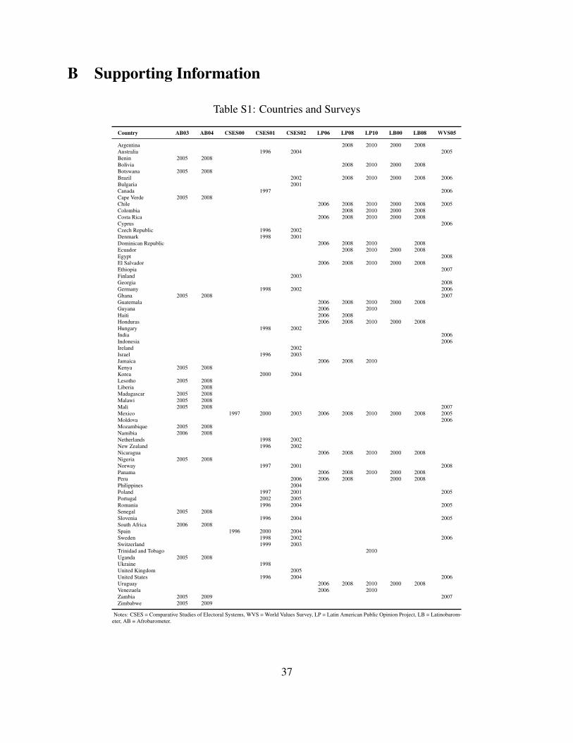
5Table S1 in the appendix containing supporting information (SI) shows the countries and surveys covered.

7

high. Therefore, a directional measure of class voting is less likely to be accurate in our low state

capacity cases. Additionally, we define class in terms of affluence and not occupation because our

theory concerns redistributive politics across a wide range of developed and developing countries.

Research on class voting in advanced industrialized countries focuses on members of the industrial

working class or manual laborers but increasingly debates how occupational categories ought to

adapt to changes in the composition of the labor force (Evans 2000). Moreover, occupation-based

definitions of class voting are hard to apply across a range of developing countries where fewer

people work in industry or the formal sector. 6

In the analysis that follows our main outcome of interest is the electoral distance in politi-

cal preferences between the top and bottom quintile. The electoral distance between the voting

preferences of two groups (m and n) is:

Electoral Distancemn =

√√√√1

2

P∑p=1

(V pm − V p

n )2 (1)

where there are P parties, and V pm is the proportion of members of group m who state they

support party p. Electoral Distance equals 0 when people in each group support the same parties

to the same degree and 1 if there is no overlap in the parties supported by people in each group in

a two-party system. We measure political preferences using responses to open-ended questions in

the surveys. The wording of specific questions on preferences, however, vary by survey.7

We measure respondents’ relative affluence within a country using asset ownership. Asset

indices are a good proxy for long-run socioeconomic status, particularly where people rely on

seasonal employment or irregular wages (Filmer & Pritchett 2001, Montgomery, Gragnolati, Burke

& Paredes 2000). We constructed a Wealth Index, which is the first principal component of a

6Mainwaring, Torcal & Somma (2015) discuss the difficulties associated with applying occupational categoriesused to measure class voting in advanced industrialized countries to Latin America.

7Wherever possible, we use the question about who the respondent would vote for if the elections were held tomor-row (Barometer surveys). Where this was not asked, we rely on who the respondent voted for in the previous election(CSES). Finally, if neither option were available we used responses to the question on which party the respondent feltclose to (LAPOP & WVS).

8

principal components analysis of assets by country and used it to place respondents into quintiles.8

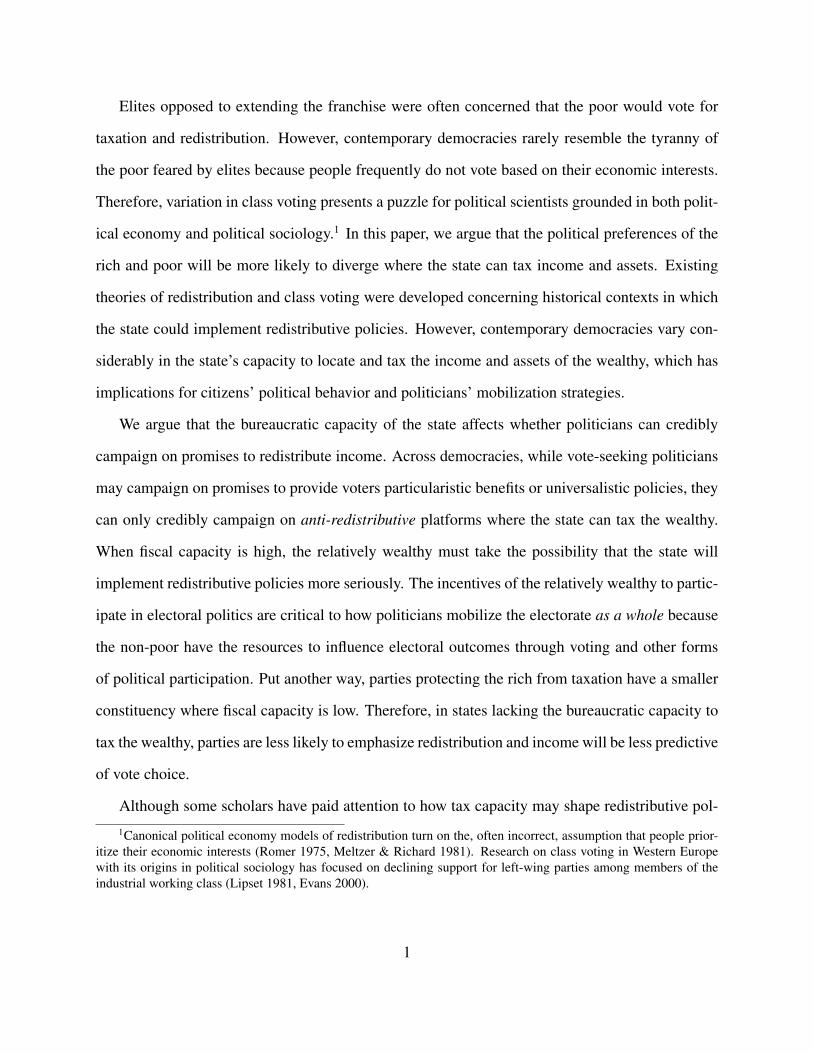
For the WVS and CSES surveys, we used income quintiles based on self-reported income.9 Figure

1 shows how Electoral Distance varies cross-nationally.

[Figure 1 about here]

Most outcomes used to measure bureaucratic capacity are partly the result of current govern-

ment policy, and bureaucratic capacity may exist even though it is unused by policymakers. We

use four standard measures of bureaucratic capacity which, to varying degrees, reflect both the

potential capability of the state and current policy choices (Hendrix 2010). First, we use a measure

of Bureaucratic Quality developed by the Political Risk Services Group (PRSG). Bureaucratic

Quality takes on a higher value in countries where the bureaucracy can govern autonomously and

if there are established mechanisms for training and staffing the civil service. Second, we use

a measure of Government Effectiveness based on experts’ perceptions of the quality of public

service (Kaufmann, Kraay & Mastruzzi 2010). Third, we include the share of government rev-

enue from direct taxes (Direct Tax/Revenue) as a measure of fiscal capacity. Finally, following

the literature on civil conflict, we use GDP per capita as a measure of state capacity (Fearon &

Laitin 2003, Hendrix 2010).

In our main regressions, we control for social and political institutions other than bureaucratic

capacity that shape class voting. We control for whether a country has proportional representation

(PR) in all regressions.10 In proportional electoral systems, a greater number of social and eco-8The assets used in each survey round are: Latinobarometer (TV, refrigerator, own home, computer, washing

machine, telephone, mobile telephone, car, second home, drinking water, hot water, sewage system, bathroom withshower, electricity), Afrobarometer (TV, radio, bicycle, motorbike, and car), and LAPOP (telephone, refrigerator,landline telephone, cellular telephone, vehicle/car, washing machine, microwave oven, motorcycle, indoor plumbing,indoor bathroom, computer, flat panel TV, internet).

9Regarding the measurement of income, as Donnelly & Pop-Eleches (2018), for example, note that there is vari-ation in how self-reported income is measured and income deciles calculated in the World Values Survey. In theempirical section that follows, we show that our findings are robust to excluding surveys with self-reported income.

10PR is measured using a dummy variable. By this definition, countries have a proportional representation electoralsystem if candidates are elected based on the percent of votes received by their party or if our sources describe thecountry as having a PR electoral system. Data on electoral laws come from the CSES and Beck, Clarke, Groff, Keefer& Walsh (2001).

9

nomic groups may be represented by a distinct political party (Cox 1987, Iversen & Soskice 2006).

Because compulsory voting may increase politicians’ incentives to campaign on redistributive plat-

forms, we include a dummy variable for the cases in which the government strictly enforces com-

pulsory voting laws (Panagopoulos 2008, Boveda 2013).

Institutions limiting politicians’ responsiveness to voters limit the potential tax exposure of

the rich. Because meaningful electoral competition may increase the policy stakes of class-based

politics, we control for the quality of a country’s democracy using its Polity Score (Marshall, Gurr

& Jaggers 2013). We also exclude from the analysis any country with a Polity Score of -4 or less.

We place people into quintiles by country, but the relative well-being of the richest and poorest

people is greater in places with more income inequality. Therefore, we control for inequality using

Gini coefficients estimated from household surveys and using gross income, i.e., income before

taxes and transfers (Milanovic 2013). We use gross rather than net income to measure inequality

because Gini coefficients constructed using net income are likely to capture a state’s tax capacity

and current redistributive policy.

Issues other than redistribution from the rich to the poor may be politically salient for reasons

unrelated to a state’s tax-raising capacity. We control for two other aspects of politics that may

reduce the political importance of redistribution. First, we control for ethnic diversity as measured

by Fearon (2003) because ethnic voting is frequently an alternative to class voting. Second, citizens

may be more likely to focus on the provision of public security than redistribution where political

violence occurs. Although there are data sources that track election-related violence, they cover

primarily developing countries. Therefore, we control for the importance of political violence

using the Homicide Rate.11

11The Homicide Rate is defined as the number of intentional homicides per 100,000 persons in the population from2003 to 2008. These data come from the United Nations Office on Drugs and Crime. The homicide rate is estimatedusing data from public health surveys and not police reports because intentional homicide is underreported.

10

We estimate the following model:

Electoral Distancej = δ + γ1Bureaucratic Qualityj + γ2PRj + γ3Concurrentj + γ4Compulsoryj

+γ5Polityj + γ6Ginij + γ7Homicidej + γ8Ethnic Fractionalizationj + ej

We present results of Feasible Generalized Least Square (FGLS) regressions on Electoral Dis-

tance .12 We used standard errors from country-level bootstrap simulations as weights for the error

correction.13 Because there are multiple surveys for some countries, our standard error estimates

are clustered by country. All continuous explanatory variables were rescaled to have a mean of 0

and a standard deviation of 0.5 to make it easier to compare continuous and binary variables.

We first present results without controls in Table 1 and find a positive relationship between

Electoral Distance and each measure of bureaucratic capacity providing evidence for our claims

that the partisan preferences of people in the top and bottom quintiles in each country differ more

when bureaucratic capacity is high.

[Table 1 about here]

In Table 2 we add the main controls we describe above. Although our four measures of state

capacity (Bureaucratic Quality, Government Effectiveness, Direct Tax/Revenue, and Log. GDP

per capita) differ, they have roughly the same substantive effect on Electoral Distance. A one

standard deviation increase in our capacity measures is associated with an increase in Electoral

Distances of between 0.04 to 0.06.14 To put this number in context, Electoral Distance in our

sample ranges from approximately 0.01 (e.g., Guatemala and Venezuela) to 0.3 (e.g., South Africa

and the United States) with a standard deviation of 0.07 (See Figure 1).15 Measuring class voting

12We use a FGSLS estimator to deal with likely heteroskedasticity in the country-level analysis and to account forthe sampling error in individual-level surveys used to generate the measure (Lewis & Linzer 2005).

13We used a 1000 samples of 100 observations each to create measures of Electoral Distance to generate standarderrors for the sampling distribution.

14This is equivalent to an increase in Electoral Distances of between 0.29 to 0.40 standard deviations. Table S2 inthe SI shows descriptive statistics

15The surveys and years these illustrative values of Electoral Distance are drawn from are: Guatemala (LAPOP

11

using the preferences of people in all five quintiles, rather than preferences of those in the top and

the bottom quintile, we find a smaller substantive effect of bureaucratic capacity on income-based

voting.16

All four models in Table 2 show a negative relationship between levels of inequality and the

Gini coefficient measured using gross income in a country. This finding is surprising as conven-

tional political economy models would predict that higher levels of inequality should be associated

with more rather than less class voting. We conjecture, but cannot show, that high pre-tax in-

equality may in part reflect low bureaucratic capacity over the long-term as weak states cannot

redistribute income.


Maybe the partisan preferences of the rich and the poor diverge because voters care about some

other trait, such as ethnicity, that is unevenly distributed along class lines. Huber & Suryanarayan

(2016), for example, find that ethnic voting is more likely when there are greater economic differ-

ences between ethnic groups. Our theoretical framework allows for the possibility that ethnicity

rather than class emerges as a basis of political mobilization where bureaucratic capacity is low.

Even where ethnicity and class overlap significantly, we would expect to see greater voting polar-

ization by income where the state can tax the wealthy. To explore the possibility that overlapping

class and ethnic cleavages drive voting polarization in some of our cases, we control for inequality

between members of different ethnic groups as measured by Baldwin & Huber (2010). Table 2

shows that bureaucratic capacity remains correlated with class voting for three out of four of our

2006), Venezuela (LAPOP 2010), United States (CSES 2004), and South Africa (Afrobarometer 2008) Though thefigure for Venezuela may seem surprising, it is consistent with what Lupu’s (2010) findings for the period just before2010.

16See Table S3 in the SI. To measure class voting use a modified version of the polarization statistic developedby Esteban & Ray (1994) to characterize income distributions. Other scholars have used variants of the Esteban-Ray polarization statistic to measure ideological, ethnic, and political polarization (Montalvo & Reynal-Querol 2005,Clark 2009, Desmet, Weber & Ortuno Ortın 2009, Huber 2012). Because we measure how much political preferencesdiverge by quintile, Voting Polarization is defined as the average of the electoral distances between any two quintilesappropriately scaled. Except for the coefficient on inequality, none of the other controls are precisely estimated acrossall four models.

12

measures, even when we control for inequality across ethnic lines. Between Group Inequality is

statistically significant in only one of the four models.


We have argued that fiscal capacity drives class voting, but the historical conditions under

which fiscal capacity was developed present one potential source of endogeneity. In older democ-

racies state-building often went with limited franchise expansion, with wealthy elites investing in

tax institutions to defer the threat of mass democratization or where democratization resulted from

elite bargains across economic sectors (Ansell & Samuels 2014, Mares & Queralt 2015). Newer

democracies present a harder test of our argument because where electoral competition preceded

the extension of the franchise, parties representing the interests of wealthy landowners and capi-

talist elites were organized before democratization giving rise to the conditions for class voting. In

Tables 4 and 5 we show that our results are robust to dividing our sample into states created before

and after 1900.17



Because countries with robust states are often wealthy ones, economic development is a po-

tential confounding variable. Of particular concern for us is the possibility that people living in

developed countries are more likely to engage in class voting for reasons other than the redis-

tributive potential of the state. The literature offers two alternative accounts of how development

may affect class voting. As we discussed in Section 1, in one account, poor people may be more

17In addition, we use an instrumental variable approach used by Dincecco & Prado (2012) in a paper exploringthe effect of state capacity on economic growth. We instrument for state capacity using the number of casualties inpremodern wars (conflicts between 1816 to 1913). This approach assumes that war casualties before World War I donot affect class voting other their impact on fiscal capacity. Instrumenting for bureaucratic capacity in this way, wefind that bureaucratic capacity predicts class voting (Table S4).

13

likely to support non-programmatic policy at low levels of development. However, scholars study-

ing voting behavior in advanced industrialized countries have also argued that economic growth

decreased class voting as voters became more interested in post-materialist issues (e.g., Inglehart

& Rabier (1986)). In Tables 6 and 7 we show that fiscal capacity and class voting are positively

correlated in countries both above and below the median GDP per capita in our sample, but the

results are weaker for developing countries.18



Even though we exclude most non-democracies from our sample, democratic responsiveness

still varies in the countries we include. We expected voting polarization by class to be greatest

where elections are consequential for policymaking. However, democratic quality – as measured

by a country’s Polity Score – does not affect voting polarization by income. When we use a stricter

threshold for what counts as a democracy, our findings are substantively the same.19

Exploring the structural and institutional correlates of class voting across a range of developed

and developing countries necessitates using cross-national survey data. Although we use survey

sources typically used in cross-national research on voting behavior, our data sources vary in qual-

ity and representativeness. We show that our findings are robust to dropping each survey source20

Additionally, as Donnelly & Pop-Eleches (2018) note about income measures in the World Values

Surveys, even the same survey might inconsistently measure a variable in different countries. In

the section that follows we examine class-based voting using sub-national data. We examine class-

based voting in the American states in the 1930s because more limited federal spending during

that period led to a closer relationship between state party systems and fiscal capacity (Chhibber &

Kollman 2004).18Table S5 in the SI also shows that our results are robust to controlling for infant mortality.19Table S6 in the SI shows the regressions in Table S6 including countries with a minimum Polity Score of 0 instead

of -4.20See Tables S7, S8, S9, S10, & S11 in the SI

14

3 Class Voting in the United States in the 1930s

We measure class voting in the U.S. using a combined dataset of 21 nationwide Gallup Polls con-

ducted in 1936 and 1937 comprising approximately 60,000 respondents. Surveys conducted by

Gallup before the 1950s used a quota-controlled sampling method to impose demographic controls

on their samples. Pollsters interviewed predetermined proportions of people from specific demo-

graphic groups. State sample sizes were chosen to match state voting patterns in the previous three

presidential elections. Within regions and cities, respondents were selected using quotas based on

age, sex, and socioeconomic status. Besides these quotas, enumerators could draw respondents

from anywhere in the community.

While the polls have significant flaws, they are valuable because they offer the only means to

study public opinion in this critical period (Verba & Schlozman 1977, Erikson & Tedin 1981, Page

& Shapiro 1982, Berinsky et al. 2011). It is worth discussing two potential sources of bias in the

sample. Surveyors’ attempts to represent specific groups rather than the population introduce the

first potential source of bias. The second source of bias arises because interviewers were given

discretion in selecting respondents who met the assigned demographic quotas (Berinsky 2006).

Gallup samples were designed to be representative of voters as opposed to the whole public –

the polls under sampled women, poor, and uneducated voters as well as Southern blacks. As

our variable of interest is class voting, the under-sampling of uneducated and poor respondents is

likely to underestimate class differences in political preferences, making our sample a harder test

of the theoretical claims of this paper. Moreover, using poststratification weights, as in Berinsky

et al. (2011), to correct for this undersampling is likely to overstate the participation of these

marginalized groups and by extension class voting in the states.

To construct the Electoral Distance variable, we use a respondent’s retrospective vote choice

in the 1936 Presidential Election. Respondents were asked, “For whom (or for which presiden-

tial candidate) did you vote in the November [1936] election?” Respondents were placed in four

15

socioeconomic categories: On Relief, Poor/Poor Plus, Average and Average Plus. These four cate-

gories were used in every survey by Gallup in 1936 and 1937. We regrouped respondents into three

categories by combining On Relief and Poor/Poor Plus into a single low-income group and used

these three groups to create the class voting measures. We do this because the distinction between

poor and on-relief respondents in this period is somewhat arbitrary. The Federal Emergency Relief

Act implemented in 1933 provided federal grants to states to meet their relief needs. As Hopkins

(1999) notes, while FERA money supported direct and work relief, states were slow to accept and

roll out relief, resulting in state-wide variation in people “On Relief”.21 Also, recipients were not

means-tested and were eligible for relief if they could provide evidence of unemployment. Taken

together, we believe it is unclear whether the share of the population “On Relief” reflects poverty

or a state’s efficacy in dealing with unemployment. Figure 2 shows how Electoral Distance varies

across states.

[Figure 2 about here]

We measure fiscal capacity as the proportion of state revenue coming from direct taxation.22 We

also use a measure of the percentage of total revenue derived from taxes of any kind (Tax/Revenue).

Though direct taxes are more difficult to collect, any taxation is an indicator of how much state

governments draw on local resources as opposed to nontax revenues, such as federal grants, during

this period (Sylla, Legler & Wallis 2006).

Table 8 shows that the political preferences of rich and poor voters diverged in states where the

government was primarily funded through taxation. As predicted, Models 1 and 2 show a positive

and significant coefficients for both Direct Tax/Revenue and Tax/Revenue.

[Table 8 about here]21FERA’s successor, the Civil Works Administration which was created in 1934, while more successful than FERA,

was still criticized for the arbitrariness of its implementation (Hopkins 1999).22In 1932, direct taxes include dates on property, businesses, income, and sometimes a special inheritance (Sylla,

Legler & Wallis 2006).

16

Race is a critical cleavage which has shaped both the American welfare state and public opinion

on redistribution (Gilens 2009, Katznelson 2005, Katznelson 2013). According to Key (1949)

the defining feature of politics in the South was the status and potential voting power of African

Americans. Race shaped policymakers’ support for and enforcement of redistributive policies

across the states (Farhang & Katznelson 2005, Lieberman & Lapinski 2001). White people are

less likely to favor redistribution where blacks were historically and are now large percentages of

the population (Glaser 1994, Acharya, Blackwell & Sen 2016).

We account for the likely effect of race on class voting by white respondents in four ways. First,

all regressions control for whether a state is in the Deep South as defined by Key (1949). Second,

we control for the proportion of a state’s population who were black.23 As Table 8 shows, the

Deep South indicator has a negative and significant coefficient suggesting that the South, which in

this period was a one-party system, had low levels of class voting. The coefficient on the % Black

variable is not significant, but this is unsurprising given this variable’s high correlation with our

indicator for the South.

Alesina & Glaeser (2004) argue that the coincidence of black racial difference and poverty

drove opposition to redistribution in the U.S. Therefore, as in the cross-national part of the paper,

we control for between-group inequality.24 Even controlling a state’s location in the Deep South

and for the share of the population who are black, we find that Between Group Inequality reduces

class voting (Table 8, Model 4). Finally, perhaps some other aspect of Southern exceptionalism

accounts for our findings. Mickey (2008) describes the South as an enclave of authoritarian rule

with the Democratic party dominating the political landscape using white-only primaries. In Ta-

ble 8, Model 5 we include only a sub-sample of Northern states. The coefficient of the Direct

23The 11 states in Key’s seminal book on southern politics include Virginia, Alabama, Tennessee, Florida, Georgia,South Carolina, Louisiana, Arkansas, North Carolina, Mississippi, and Texas.

24We measured Between Group Inequality using total family income in 1950 for whites and blacks only using theU.S. Integrated Public Use Microdata Series (IPUMS) (Ruggles, Trent, Genadek, Goeken, Schroeder & Sobek 2010).Although this date occurs after the survey, the 1930 sample census includes no measure of total family income, onlyone of educational attainment. Though not ideal, this measure is justifiable because racial inequality changes littleover time.

17

Tax/Revenue variable is larger in magnitude if only Northern states are included as is the negative

coefficient on Between Group Inequality.

Theories of class voting suggest that political mobilization by the working class and inequal-

ity increase demand for redistribution. The industrial working class was a core constituency for

left-wing parties. Authors studying the New Deal Era legislation and labor movements have em-

phasized the highly contentious role of labor in redistributive politics before and during the Civil

Rights Movement (Lichtenstein 1930, Brinkley 2011). Because demand for redistribution may be

higher in states with high concentrations of industrial workers, we include the proportion of the

workforce engaged in manufacturing in 1930 in all regressions. Contrary to expectation, neither

inequality nor the percent of the workforce in manufacturing predict divergent political preferences

along class lines.25

The class categories chosen by Gallup constrains us, but our findings are robust to alternative

ways of measuring class voting and political preferences. As in the cross-national section, our

results are substantively unchanged if we use Voting Polarization across all three income classes

rather than Electoral Distance as our outcome.26 In Table 8 we placed people classified by survey-

ors as “Poor” and those categorized as “On Relief,” into the same income category, and our results

are the same when we separate those two categories.27 Finally, respondents may have partisan

preferences that are not reflected in their stated vote choice because of strategic voting. We created

the Electoral Distance measure using party affiliation for about 3,000 respondents. To capture

party affiliation, respondents were asked “Do you regard yourself as a Republican, Democrat, or

a Socialist?” Measuring electoral distance in party affiliation rather than vote choice we find that

fiscal capacity and Electoral Distance are positively correlated.28

25Because organized labor (rather than just labor in the manufacturing sector) might be key to organizing votersby class; we include a control for Union Density. The variable is measured as the proportion of unionized laborersto total non-agricultural wage labor and salaried employees in a state in 1939 as reported in Troy (1957). Table S12shows that Union Density is not significant at conventional thresholds.

26See Table S13 in the SI.27See Table S14 in the SI.28See Table S15 in the SI.

18

4 Conclusion

We have argued that the political preferences of the rich and poor diverge as a state’s capacity to

raise revenue through taxation increases. While parties often have a range of strategies they can use

to attract low-income voters, they are more constrained in how they can use tax policy to attract

wealthy voters. Where fiscal capacity is high, rich voters must take the threat of redistribution

seriously and are more motivated to participate in politics and more likely to respond favorably

to conservative economic platforms. In turn, where politicians can credibly promise to tax the

wealthy, they are more likely to campaign on platforms that allow voters to vote their economic

interests on redistribution.

Using both contemporary cross-national data and subnational public opinion data from the

United States in the 1930s we show how bureaucratic capacity shapes class voting in both these

spheres. Our cross-national and U.S. findings are robust to multiple measures of how preferences

diverge by class. Ethnicity influences preferences for redistribution both directly, through people’s

willingness to support redistribution to ethnic others, and indirectly, through its effect on how

politicians create coalitions to win elections. Therefore, in both the U.S. and cross-nationally, we

include a measure of ethnic composition. Because likely beneficiaries of redistribution may be

concentrated in one ethnic group, we show that our results are robust to including a measure of

economic inequality between ethnic groups.

Even though our primary goal is to argue that bureaucratic capacity partially explains where

class voting predominates, our theory has predictions regarding when politicians will emphasize

redistribution even in places where class is a political cleavage. In established democracies, parties

moderate their platforms in response to changes in voter preferences (See Adams (2012)). For

example, Tavits & Potter (2015) argue that inequality, which increases demand for redistribution,

leads right-wing parties to emphasize values rather than economic interests as inequality increases.

Although no prior work has shown that changes in fiscal capacity lead right-wing parties to mod-

19

erate or de-emphasize their stances on redistribution, our theory predicts that they will do so.

We show that racial inequality in the U.S. states is negatively correlated with class voting during

the period we study, even in the North. While there is an extensive literature on the effects of racial

composition on both racial attitudes and voting behavior at the local level, the relationship between

racial economic inequality and class voting remains relatively understudied (Key 1949, Bledsoe,

Welch, Sigelman & Combs 1995, Carsey 1995).29 A natural extension of this paper would be to

explore how changes in racial inequality have affected class voting since the 1930s.

Besides contributing to research on class voting, this paper also has implications for research

on accountability in rentier states. The literature on the resource curse suggests that nontax rev-

enue produces poor governance because, absent taxation, citizens are uninformed or politically

disengaged (Ross 2004). Our argument suggests a different mechanism linking resource rents and

accountability. As the wealthy can more easily demand accountability, poor governance may arise

in rentier states because politicians have little incentive to stress fiscal stewardship to citizens best

placed to demand political accountability.

29Though Gay (2006) shows that African Americans have more hostile attitudes towards Latinos in neighborhoodswhere Latinos are better off.

20

ReferencesAcharya, Avidit, Matthew Blackwell & Maya Sen. 2016. “The Political Legacy of American

Slavery.” The Journal of Politics 78(3):621–641.

Adams, James. 2012. “Causes and Electoral Consequences of Party Policy Shifts in MultipartyElections: Theoretical Results and Empirical Evidence.” Annual Review of Political Science15(1):401–419.

AIPO, American Institute of Public Opinion. 1937. “1936-1937 Composite Gallup Poll.”.

Alesina, Alberto & Edward Glaeser. 2004. Fighting Poverty in the US and Europe: A World ofDifference. New York: Oxford University Press.

Alesina, Alberto & Eliana La Ferrara. 2005. “Preferences for redistribution in the land of oppor-tunities.” Journal of Public Economics 89(5–6):897–931.

Amat, Francesc & Pablo Beramendi. 2018. “Democracy Under High Inequality: Political Partici-pation and Public Goods.”.

Ansell, Ben W & David J Samuels. 2014. Inequality and democratization: an elite-competitionapproach. Cambridge University Press.

Baldwin, Kate & John D. Huber. 2010. “Economic versus Cultural Differences: Forms of EthnicDiversity and Public Goods Provision.” American Political Science Review 104(04):644–662.

Bates, Robert & Da-Tsiang Donald Lien. 1985. “A Note on Taxation Development and Represen-tative Government.” Politics and Society 14(1):53–70.

Beck, Thorsten, George Clarke, Alberto Groff, Philip Keefer & Patrick Walsh. 2001. “New toolsin comparative political economy: The Database of Political Institutions.” World Bank Eco-nomic Review. 15(1).

Becker, Gary S & Casey B Mulligan. 2003. “Deadweight Costs and the Size of Government.”Journal of Law and Economics 46:293.

Berinsky, Adam J. 2006. “American Public Opinion in the 1930s and 1940s: The Analysis ofQuota-Controlled Sample Survey Data.” Public Opinion Quarterly 70(4):499–529.

Berinsky, Adam J, Eleanor Neff Powell, Eric Schickler & Ian Brett Yohai. 2011. “Revisiting PublicOpinion in the 1930s and 1940s.” PS: Political Science & Politics 44(03):515–520.

Bledsoe, Timothy, Susan Welch, Lee Sigelman & Michael Combs. 1995. “Residential Contextand Racial Solidarity among African Americans.” American Journal of Political Science39(2):434–458.

Boix, Carles. 2003. Democracy and Redistribution. New York: Cambridge University Press.

21

Boix, Carles. 2009. The Emergence of Parties and Party Systems. In The Oxford Handbook ofComparative Politics, ed. Carles Boix & Susan C. Stokes. Oxford University Press.

Boveda, Karina C. 2013. “Making People Vote: The Political Economy of Compulsory VotingLaws.”.

Brinkley, Alan. 2011. The end of reform: New Deal liberalism in recession and war. Vintage.

Caramani, Daniele. 2004. “The nationalization of politics : the formation of national electoratesand party systems in Western Europe.”.

Carsey, Thomas M. 1995. “The Contextual Effects of Race on White Voter Behavior: The 1989New York City Mayoral Election.” The Journal of Politics 57(1):221–228.

Chhibber, Pradeep & Ken Kollman. 2004. The Formation of National Party Systems: Federalismand Party Competition in Canada, Great Britain, India, and the United States. Princeton,NJ: Princeton University Press.

Clark, Tom S. 2009. “Measuring Ideological Polarization on the United States Supreme Court.”Political Research Quarterly 62(1):146–157.

Cox, Gary W. 1987. The efficient secret : the cabinet and the development of political parties inVictorian England. Political economy of institutions and decisions Cambridge ; New York:Cambridge University Press. Gary W. Cox. ill. ; 24 cm. Includes indexes.

De La O, Ana L. & Jonathan A. Rodden. 2008. “Does Religion Distract the Poor?: Income andIssue Voting Around the World.” Comparative Political Studies 41(4):437–476.

Desmet, Klaus, Shlomo Weber & Ignacio Ortuno Ortın. 2009. “Linguistic Diversity and Redistri-bution.” Journal of the European Economic Association 7(6):1291–1318.

Dincecco, Mark & Mauricio Prado. 2012. “Warfare, fiscal capacity, and performance.” Journal ofEconomic Growth 17(3):171–203.

Donnelly, Michael J & Grigore Pop-Eleches. 2018. “Income Measures in Cross-National Surveys:Problems and Solutions.” Political Science Research and Methods 6(2):355363.

Dunning, Thad. 2008. Crude Democracy: Natural Resource Wealth and Political Regimes. NewYork: Cambridge University Press.

Erikson, Robert S. & Kent L. Tedin. 1981. “The 1928-1936 Partisan Realignment: The Case forthe Conversion Hypothesis.” American Political Science Review 75(04):951–962.

Esteban, Joan-Maria & Debraj Ray. 1994. “On the Measurement of Polarization.” Econometrica62(4):819–851.

Evans, Geoffrey. 2000. “The Continued Significance of Class Voting.” Annual Review of PoliticalScience 3:401–417.

22

Evans, Geoffrey. 2006. “The Social Bases of Political Divisions in Post-Communist Eastern Eu-rope.” Annual review of sociology 32(1):245–270.

Farhang, Sean & Ira Katznelson. 2005. “The southern imposition: Congress and labor in the newdeal and fair deal.” Studies in American Political Development 19(01):1–30.

Fearon, James D. 2003. “Ethnic Structure and Cultural Diversity around the World: A Cross-National Data Set on Ethnic Groups.” Journal of Economic Growth 8:195–222.

Fearon, James D. & David D. Laitin. 2003. “Ethnicity, Insurgency, and Civil War.” AmericanPolitical Science Review 97(1):75–90.

Fernandez, Raquel & Gilat Levy. 2008. “Diversity and redistribution.” Journal of Public Eco-nomics 92(5-6):925–943.

Filmer, Deon & Lant Pritchett. 2001. “Estimating Wealth Effects Without Expenditure Dataor Tears: An Application to Educational Enrollments in States of India.” Demography38(1):115–32.

Gay, Claudine. 2006. “Seeing Difference: The Effect of Economic Disparity on Black AttitudesToward Latinos.” American Journal of Political Science 50(4):982997.

Gilens, Martin. 2009. Why Americans hate welfare: Race, media, and the politics of antipovertypolicy. University of Chicago Press.

Glaser, James M. 1994. “Back to the Black Belt: Racial Environment and White Racial Attitudesin the South.” The Journal of Politics 56(1):21–41.

Hendrix, Cullen S. 2010. “Measuring state capacity: Theoretical and empirical implications forthe study of civil conflict.” Journal of Peace Research 47(3):273–285.

Hopkins, June. 1999. “The Road Not Taken: Harry Hopkins and the New Deal Work Relief.”Presidential Studies Quarterly 29(2):306–316.

Huber, John D. 2012. “Measuring Ethnic Voting: Do Proportional Electoral Laws Politicize Eth-nicity?” American Journal of Political Science 56(4):986–1001.

Huber, John D. 2017. Exclusion by Elections. Cambridge University Press.

Huber, John D. & Michael M. Ting. 2013. “Redistribution, Pork, and Elections.” Journal of theEuropean Economic Association 11(6):1382–1403.

Huber, John D. & Pavithra Suryanarayan. 2016. “Ethnic Inequality and the Ethnification of Politi-cal Parties: Evidence from India.” World Politics 68(1).

Inglehart, Ronald & Jacques-Rene Rabier. 1986. “Political realignment in advanced industrialsociety: from class-based politics to quality-of-life politics.” Government and Opposition21(4):456–479.

23

Iversen, Torben & David Soskice. 2006. “Electoral Institutions and the Politics of Coalitions:Why Some Democracies Redistribute More Than Others.” American Political Science Review100(02):165–181.

Jusko, Karen Long. 2017. Who Speaks for the Poor?: Electoral Geography, Party Entry, andRepresentation. Cambridge University Press.

Kasara, Kimuli & Pavithra Suryanarayan. 2015. “When Do the Rich Vote Less Than the Poorand Why? Explaining Turnout Inequality across the World.” American Journal of PoliticalScience 59(3):613–627.

Katznelson, Ira. 2005. When affirmative action was white: An untold history of racial inequalityin twentieth-century America. WW Norton & Company.

Katznelson, Ira. 2013. Fear itself: The new deal and the origins of our time. WW Norton &Company.

Kaufmann, Daniel, Aart Kraay & Massimo Mastruzzi. 2010. “The Worldwide Governance In-dicators: Methodology and Analytical Issues.” World Bank Policy Research Working Paper5430.

Key, V. O. 1949. Southern Politics in State and Nation. New ed. Knoxville: University of Ten-nessee Press.

Lewis, Jeffrey B. & Drew A. Linzer. 2005. “Estimating Regression Models in Which the Depen-dent Variable Is Based on Estimates.” Political Analysis 13(4):345–364.

Lichtenstein, Nelson. 1930. “From corporatism to collective bargaining: organized labor and theeclipse of social democracy in the postwar era.” The rise and fall of the New Deal Order1980(122):140–45.

Lieberman, Robert C. & John S. Lapinski. 2001. “American Federalism, Race and the Adminis-tration of Welfare.” British Journal of Political Science 31(2):303–329.

Lipset, Seymour M. 1981. Political Man: The Social Basis of Politics. 2nd ed. ed. Baltimore:Johns Hopkins University Press.

Lipset, Seymour M. & Stein Rokkan. 1967. Cleavage Structures, Party Systems and Voter, Align-ments: An Introduction. In Party Systems and Voter Alignments: Cross-National Perspec-tives, ed. Seymour M. Lipset & Stein Rokkan. New York: Free Press pp. 1–63.

Lupu, Noam. 2010. “Who Votes for chavismo?: Class Voting in Hugo Chvez’s Venezuela.” LatinAmerican Research Review 45(1):7–32.

Mainwaring, Scott, Mariano Torcal & Nicolas M Somma. 2015. The Left and the Mobilizationof Class Voting in Latin America. In The Latin American Voter, ed. Ryan Carlin, MatthewSinger & Elizabeth Zechmeister. Ann Arbor: University of Michigan Press pp. 69–98.

24

Mares, Isabela & Didac Queralt. 2015. “The non-democratic origins of income taxation.” Com-parative Political Studies 48(14):1974–2009.

Marshall, Monty G., Ted R. Gurr & Keith Jaggers. 2013. “Polity IV Project: Political RegimeCharacteristics and Transitions, 1800-2013.”.

Meltzer, A. H. & S. F. Richard. 1981. “A Rational Theory of the Size of Government.” Journal ofPolitical Economy 89(5):914–27.

Mickey, Robert W. 2008. “The Beginning of the End for Authoritarian Rule in America: Smith v.Allwright and the Abolition of the White Primary in the Deep South, 1944–1948.” Studies inAmerican political development 22(02):143–182.

Milanovic, Branko L. 2013. “All the Ginis Database.”.

Milkis, Sidney M. 1993. The president and the parties : the transformation of the American partysystem since the New Deal. New York :: Oxford University Press.

Montalvo, Jose G. & Marta Reynal-Querol. 2005. “Ethnic Polarization, Potential Conflict, andCivil Wars.” American Economic Review 95(3):796–816.

Montgomery, Mark R., Michele Gragnolati, Kathxn A. Burke & Edmundo Paredes. 2000. “Mea-suring Living Standards with Proxy Variables.” Demography 37(2):155–174.

Nathan, Noah L. 2016. “Does Participation Reinforce Patronage? Policy Preferences, Turnout andClass in Urban Ghana.” British Journal of Political Science pp. 1–27.

Page, Benjamin I & Robert Y Shapiro. 1982. “Changes in Americans’ policy preferences, 1935–1979.” Public Opinion Quarterly 46(1):24–42.

Panagopoulos, Costas. 2008. “The Calculus of Voting in Compulsory Voting Systems.” PoliticalBehavior 30(4):455–467.

Przeworski, Adam & John Sprague. 1986. Paper Stones: A History of Electoral Socialism.Chicago: University of Chicago Press.

Roemer, John E. 1998. “Why the poor do not expropriate the rich: an old argument in new garb.”Journal of Public Economics 70(3):399–424.

Romer, Thomas. 1975. “Individual welfare, majority voting, and the properties of a linear incometax.” Journal of Public Economics 4(2):163–185.

Ross, Michael. 2004. “Does Taxation Lead to Representation?” British Journal of Political Science34(2):229–249.

Ruggles, Steven, Alexander Trent, Katie Genadek, Ronald Goeken, Matthew B. Schroeder &Matthew Sobek. 2010. “Integrated Public Use Microdata Series: Version 5.0.”.

25

Sandbrook, Richard. 1977. “The Political Potential of African Urban Workers.” Canadian Journalof African Studies 11(3):411–433.

Schattschneider, E.E. 1960. The Semisovereign People: A Realist’s View of Democracy in America.Fort Worth: Harcourt Brace Jovanovich College Publishers.

Scheve, Kenneth & David Stasavage. 2006. “Religion and Preferences for Social Insurance.”Quarterly Journal of Political Science 1(3):255–286.

Shayo, Moses. 2009. “A Model of Social Identity with an Application to Political Economy:Nation, Class, and Redistribution.” American Political Science Review 103(02):147–174.

Sklar, Richard L. 1979. “The Nature of Class Domination in Africa.” Journal of Modern AfricanStudies 17(4):53152.

Soifer, Hillel D. 2013. “State Power and the Economic Origins of Democracy.” Studies in Com-parative International Development 48(1):1–22.

Stokes, Donald E. 1967. Parties and the nationalization of electoral forces. In The Americanparty systems: stages of political development, ed. William Nisbet Chambers, Walter DeanBurnham & Frank J. Sorauf. New York: Oxford University Press.

Stokes, Susan C. 2005. “Perverse Accountability: A Formal Model of Machine Politics withEvidence from Argentina.” American Journal of Political Science 99(3):315–325.

Sylla, Richard E., John B. Legler & John Wallis. 2006. “State and Local Government [UnitedStates]: Sources and Uses of Funds, Census Statistics, Twentieth Century [Through 1982].”.

Tavits, Margit & Joshua D. Potter. 2015. “The Effect of Inequality and Social Identity on PartyStrategies.” American Journal of Political Science 59(3):744–758.

Verba, Sidney & Kay Lehman Schlozman. 1977. “Unemployment, class consciousness, and radicalpolitics: what didn’t happen in the thirties.” The Journal of Politics 39(02):291–323.

Vernby, Kare & Henning Finseraas. 2010. “Xenophobia and Left Voting.” Politics & Society38(4):490–516.

Weitz-Shapiro, Rebecca. 2012. “What Wins Votes: Why Some Politicians Opt Out of Clientelism.”American Journal of Political Science 56(3):568–583.

26

A Figures & Tables

Figure 1: Electoral Distance Across the World

27

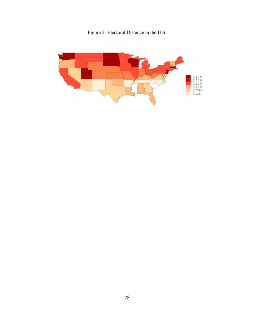
Figure 2: Electoral Distance in the U.S.

28

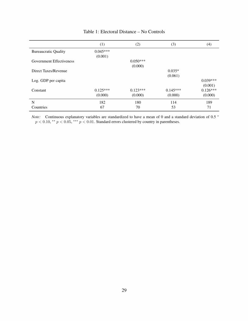
Table 1: Electoral Distance – No Controls

(1) (2) (3) (4)

Bureaucratic Quality 0.045***(0.001)

Government Effectiveness 0.050***(0.000)

Direct Taxes/Revenue 0.035*(0.061)

Log. GDP per capita 0.039***(0.001)

Constant 0.125*** 0.123*** 0.145*** 0.126***(0.000) (0.000) (0.000) (0.000)

N 182 180 114 189Countries 67 70 53 71

Note: Continuous explanatory variables are standardized to have a mean of 0 and a standard deviation of 0.5 ∗

p < 0.10, ∗∗ p < 0.05, ∗∗∗ p < 0.01. Standard errors clustered by country in parentheses.

29

Table 2: Electoral Distance

(1) (2) (3) (4)

Bureaucratic Quality 0.040**(0.011)


Direct Taxes/Revenue 0.054**(0.025)

Log. GDP per capita 0.042**(0.050)

PR -0.026 -0.030 -0.015 -0.032(0.180) (0.100) (0.458) (0.113)

Compulsory Voting 0.017 0.009 -0.070 0.010(0.391) (0.661) (0.126) (0.608)

Concurrent Elections -0.022 -0.017 -0.009 -0.022(0.137) (0.171) (0.680) (0.110)

Polity -0.010 -0.016 -0.020 -0.007(0.534) (0.284) (0.400) (0.620)

Gini (Gross) -0.034** -0.033* -0.035* -0.038**(0.041) (0.052) (0.070) (0.027)

Homicide Rate 0.017 0.024 0.030* 0.016(0.375) (0.220) (0.073) (0.457)

Ethnic Fractionalization -0.012 -0.009 -0.036** -0.004(0.424) (0.539) (0.037) (0.808)

Constant 0.153*** 0.152*** 0.156*** 0.159***(0.000) (0.000) (0.000) (0.000)

N 163 159 93 167Countries 58 59 42 60



30

Table 3: Electoral Distance – Controlling for BGI

(1) (2) (3) (4)

Bureaucratic Quality 0.032(0.220)

Government Effectiveness 0.041*(0.098)



Between Group Inequality 0.040* 0.030 0.025 0.023(0.082) (0.277) (0.442) (0.366)

PR -0.009 -0.018 -0.002 -0.018(0.668) (0.455) (0.931) (0.428)

Compulsory Voting -0.054** -0.059** -0.112* -0.049**(0.038) (0.026) (0.087) (0.046)

Concurrent Elections 0.013 0.014 0.016 0.011(0.579) (0.519) (0.643) (0.607)

Polity 0.049* 0.049* 0.011 0.035(0.079) (0.087) (0.789) (0.131)

Gini (Gross) -0.040* -0.046* -0.038 -0.041*(0.086) (0.052) (0.142) (0.064)

Homicide Rate 0.027 0.035 0.034 0.030(0.262) (0.156) (0.154) (0.177)

Ethnic Fractionalization -0.026 -0.019 -0.047 0.001(0.302) (0.434) (0.171) (0.965)

Constant 0.137*** 0.138*** 0.140*** 0.144***(0.000) (0.000) (0.000) (0.000)

N 60 60 42 63Countries 38 38 29 40



31

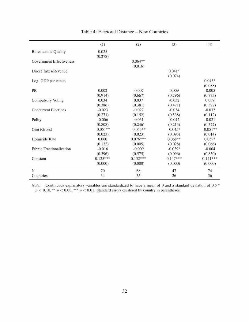
Table 4: Electoral Distance – New Countries

(1) (2) (3) (4)


Government Effectiveness 0.064**(0.016)


Log. GDP per capita 0.043*(0.088)

PR 0.002 -0.007 0.009 -0.005(0.914) (0.667) (0.796) (0.773)



Polity -0.006 -0.031 -0.042 -0.021(0.808) (0.246) (0.213) (0.322)

Gini (Gross) -0.051** -0.053** -0.045* -0.051**(0.023) (0.023) (0.093) (0.014)

Homicide Rate 0.060 0.076*** 0.068** 0.059*(0.122) (0.005) (0.028) (0.066)

Ethnic Fractionalization -0.016 -0.009 -0.039* -0.004(0.396) (0.575) (0.096) (0.830)

Constant 0.125*** 0.132*** 0.147*** 0.141***(0.000) (0.000) (0.000) (0.000)

N 70 68 47 74Countries 34 35 26 36



32

Table 5: Electoral Distance – Older Countries

(1) (2) (3) (4)




Log. GDP per capita 0.050(0.116)

Constant 0.124*** 0.122*** 0.145*** 0.118***(0.000) (0.000) (0.000) (0.000)

N 98 95 51 98Countries 27 27 19 27


p < 0.10, ∗∗ p < 0.05, ∗∗∗ p < 0.01. Standard errors clustered by country in parentheses. Compulsory Voting isexcluded from these regressions because, under these definitions, no established democracies for which we havesome data on state capacity also have compulsory voting laws.

33

Table 6: Electoral Distance – Developed Countries

(1) (2) (3) (4)





PR -0.002 -0.028 -0.032 -0.004(0.960) (0.583) (0.520) (0.929)


Concurrent Elections -0.023 -0.009 0.033 -0.025(0.347) (0.729) (0.494) (0.291)

Polity -0.018 -0.026 -0.039 -0.011(0.260) (0.144) (0.175) (0.513)

Gini (Gross) 0.003 -0.009 -0.037 0.006(0.909) (0.791) (0.327) (0.892)

Homicide Rate 0.039 0.046* 0.060 0.031(0.176) (0.072) (0.173) (0.359)

Ethnic Fractionalization -0.017 -0.015 -0.050 -0.011(0.585) (0.657) (0.263) (0.702)

Constant 0.123*** 0.130*** 0.162*** 0.101**(0.005) (0.005) (0.002) (0.024)

N 86 79 48 86Countries 28 28 19 28



34

Table 7: Electoral Distance – Developing Countries

(1) (2) (3) (4)

Bureaucratic Quality -0.016(0.487)

Government Effectiveness 0.063(0.113)

Direct Taxes/Revenue 0.028(0.403)


Constant 0.104*** 0.136*** 0.139*** 0.119***(0.000) (0.000) (0.000) (0.000)

N 79 85 49 86Countries 32 35 26 36



35

Table 8: U.S.:Electoral Distance

(1) (2) (3) (4) (5)All All All All North

Direct Tax/Revenue 0.102** 0.113** 0.113** 0.146***(0.013) (0.021) (0.018) (0.006)

Tax/Revenue 0.092**(0.034)

Gini -0.024 -0.020 -0.019(0.682) (0.722) (0.759)

Between Group Inequality -0.139* -0.176*(0.088) (0.062)

Deep South -0.169** -0.158** -0.174** -0.139*(0.024) (0.040) (0.024) (0.073)

% Black -0.058 -0.066 -0.051 0.029 -0.054(0.409) (0.363) (0.487) (0.729) (0.663)

% Manufacturing Employment 0.005 0.007 0.015 -0.007 -0.024(0.896) (0.870) (0.746) (0.880) (0.635)

Constant 0.281*** 0.278*** 0.283*** 0.272*** 0.246***(0.000) (0.000) (0.000) (0.000) (0.000)

N 46 46 46 46 37



36

B Supporting Information

Table S1: Countries and Surveys

Country AB03 AB04 CSES00 CSES01 CSES02 LP06 LP08 LP10 LB00 LB08 WVS05

Argentina 2008 2010 2000 2008Australia 1996 2004 2005Benin 2005 2008Bolivia 2008 2010 2000 2008Botswana 2005 2008Brazil 2002 2008 2010 2000 2008 2006Bulgaria 2001Canada 1997 2006Cape Verde 2005 2008Chile 2006 2008 2010 2000 2008 2005Colombia 2008 2010 2000 2008Costa Rica 2006 2008 2010 2000 2008Cyprus 2006Czech Republic 1996 2002Denmark 1998 2001Dominican Republic 2006 2008 2010 2008Ecuador 2008 2010 2000 2008Egypt 2008El Salvador 2006 2008 2010 2000 2008Ethiopia 2007Finland 2003Georgia 2008Germany 1998 2002 2006Ghana 2005 2008 2007Guatemala 2006 2008 2010 2000 2008Guyana 2006 2010Haiti 2006 2008Honduras 2006 2008 2010 2000 2008Hungary 1998 2002India 2006Indonesia 2006Ireland 2002Israel 1996 2003Jamaica 2006 2008 2010Kenya 2005 2008Korea 2000 2004Lesotho 2005 2008Liberia 2008Madagascar 2005 2008Malawi 2005 2008Mali 2005 2008 2007Mexico 1997 2000 2003 2006 2008 2010 2000 2008 2005Moldova 2006Mozambique 2005 2008Namibia 2006 2008Netherlands 1998 2002New Zealand 1996 2002Nicaragua 2006 2008 2010 2000 2008Nigeria 2005 2008Norway 1997 2001 2008Panama 2006 2008 2010 2000 2008Peru 2006 2006 2008 2000 2008Philippines 2004Poland 1997 2001 2005Portugal 2002 2005Romania 1996 2004 2005Senegal 2005 2008Slovenia 1996 2004 2005South Africa 2006 2008Spain 1996 2000 2004Sweden 1998 2002 2006Switzerland 1999 2003Trinidad and Tobago 2010Uganda 2005 2008Ukraine 1998United Kingdom 2005United States 1996 2004 2006Uruguay 2006 2008 2010 2000 2008Venezuela 2006 2010Zambia 2005 2009 2007Zimbabwe 2005 2009

Notes: CSES = Comparative Studies of Electoral Systems, WVS = World Values Survey, LP = Latin American Public Opinion Project, LB = Latinobarom-eter, AB = Afrobarometer.

37

Table S2: Descriptive Statistics

World Mean SD Min Max N

Electoral Distance 0.13 0.07 0.01 0.34 189Bureaucratic Quality 0.59 0.26 0 1 204Government Effectiveness 0.16 0.9 -1.61 2.26 201Direct Taxes/Revenue 0.29 0.11 0.1 0.66 125Log. GDP per capita 8.08 1.42 5.02 10.64 211PR 0.8 0.4 0 1 211Compulsory Voting 0.04 0.2 0 1 211Concurrent Elections 0.46 0.5 0 1 211Polity 1.39 4.19 -3.97 10 211Gini (Gross) 45 9.82 23.4 73.5 189Homicide Rate 14.34 14.75 0.5 68 211Ethnic Fractionalization 0.44 0.24 0 0.93 209Between Group Inequality 0.04 0.03 0 0.13 74Infant Mortality 26.12 24.25 2.7 106.2 211

Cross-National Mean SD Min Max N

Electoral Distance 0.25 0.15 0 0.58 46Direct Tax/Revenue 0.02 0.02 0 0.11 48Tax/Revenue 0.04 0.05 0 0.33 48Gini 0.45 0.06 0.33 0.65 48Between Group Inequality 0.04 0.05 0 0.2 48Deep South 0.22 0.42 0 1 51% Black 0.1 0.14 0 0.5 48% Manufacturing Employment 0.06 0.04 0.01 0.18 48% Union Membership (1939) 17.13 8.99 4 41.7 49

38

Table S3: Voting Polarization

(1) (2) (3) (4)





PR -0.009* -0.011** -0.004 -0.010*(0.065) (0.025) (0.484) (0.083)

Compulsory Voting 0.002 0.000 -0.021* 0.001(0.760) (0.953) (0.091) (0.890)

Concurrent Elections -0.008* -0.007* -0.006 -0.008*(0.098) (0.097) (0.385) (0.079)

Polity -0.002 -0.004 -0.003 -0.001(0.688) (0.417) (0.678) (0.835)

Gini (Gross) -0.012*** -0.013*** -0.014** -0.013***(0.006) (0.005) (0.015) (0.002)

Homicide Rate 0.003 0.005 0.006 0.003(0.533) (0.305) (0.218) (0.586)

Ethnic Fractionalization -0.005 -0.003 -0.004 -0.003(0.260) (0.411) (0.418) (0.435)

Constant 0.060*** 0.061*** 0.059*** 0.061***(0.000) (0.000) (0.000) (0.000)

N 165 161 94 169Countries 58 60 42 60



39

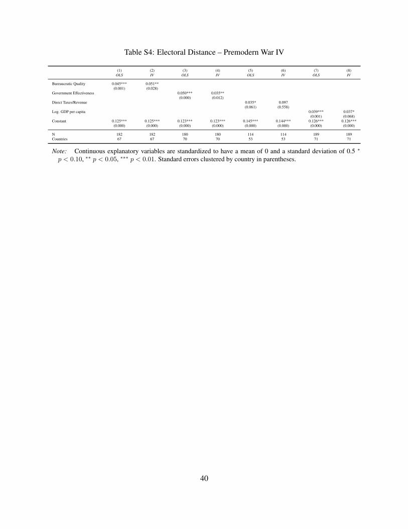
Table S4: Electoral Distance – Premodern War IV

(1) (2) (3) (4) (5) (6) (7) (8)OLS IV OLS IV OLS IV OLS IV

Bureaucratic Quality 0.045*** 0.051**(0.001) (0.028)

Government Effectiveness 0.050*** 0.035**(0.000) (0.012)

Direct Taxes/Revenue 0.035* 0.097(0.061) (0.558)

Log. GDP per capita 0.039*** 0.037*(0.001) (0.068)

Constant 0.125*** 0.125*** 0.123*** 0.123*** 0.145*** 0.144*** 0.126*** 0.126***(0.000) (0.000) (0.000) (0.000) (0.000) (0.000) (0.000) (0.000)

N 182 182 180 180 114 114 189 189Countries 67 67 70 70 53 53 71 71



40

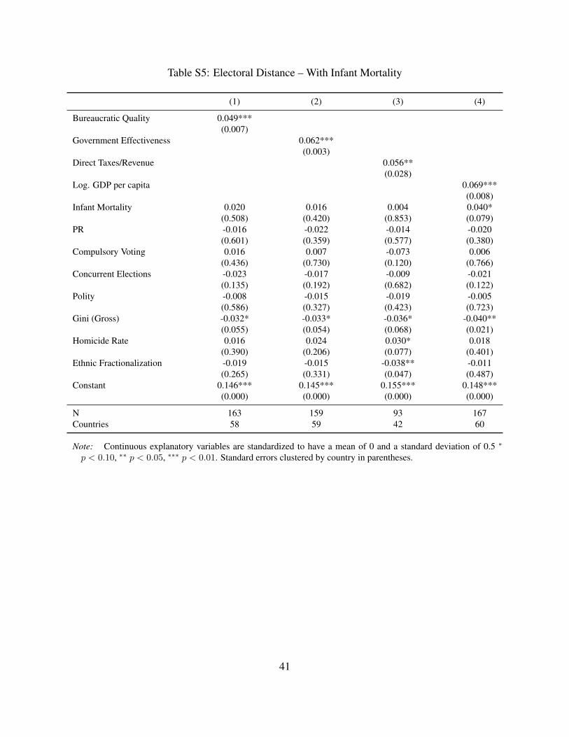
Table S5: Electoral Distance – With Infant Mortality

(1) (2) (3) (4)





Infant Mortality 0.020 0.016 0.004 0.040*(0.508) (0.420) (0.853) (0.079)

PR -0.016 -0.022 -0.014 -0.020(0.601) (0.359) (0.577) (0.380)



Polity -0.008 -0.015 -0.019 -0.005(0.586) (0.327) (0.423) (0.723)

Gini (Gross) -0.032* -0.033* -0.036* -0.040**(0.055) (0.054) (0.068) (0.021)

Homicide Rate 0.016 0.024 0.030* 0.018(0.390) (0.206) (0.077) (0.401)


Constant 0.146*** 0.145*** 0.155*** 0.148***(0.000) (0.000) (0.000) (0.000)

N 163 159 93 167Countries 58 59 42 60



41

Table S6: Electoral Distance – Altering the Threshold for Democracies

(1) (2) (3) (4)





PR -0.003 -0.022 -0.009 0.006(0.943) (0.618) (0.864) (0.888)


Concurrent Elections -0.007 0.016 -0.012 -0.012(0.829) (0.630) (0.756) (0.692)

Polity 0.002 0.001 -0.005 0.006(0.924) (0.974) (0.853) (0.793)

Gini (Gross) -0.008 -0.042 -0.009 -0.020(0.786) (0.213) (0.821) (0.529)

Homicide Rate 0.014 0.041 0.002 0.018(0.514) (0.120) (0.945) (0.477)

Ethnic Fractionalization 0.014 0.027 -0.006 0.027(0.538) (0.218) (0.751) (0.232)

Constant 0.115*** 0.120*** 0.143*** 0.109***(0.004) (0.004) (0.006) (0.008)

N 75 71 50 75Countries 29 29 21 29



42

Table S7: Electoral Distance Without Afrobarometer

(1) (2) (3) (4)



Direct Taxes/Revenue 0.043(0.137)


PR -0.048 -0.050 -0.046 -0.048(0.138) (0.110) (0.172) (0.150)



Polity -0.022* -0.021 -0.031 -0.013(0.098) (0.139) (0.194) (0.338)

Gini (Gross) -0.037* -0.039* -0.039 -0.042*(0.076) (0.084) (0.255) (0.071)

Homicide Rate 0.005 0.012 0.020 0.004(0.819) (0.595) (0.417) (0.865)


Constant 0.169*** 0.169*** 0.175*** 0.168***(0.000) (0.000) (0.000) (0.000)

N 136 128 70 136Countries 47 46 31 47



43

Table S8: Electoral Distance Without CSES

(1) (2) (3) (4)



Direct Taxes/Revenue 0.064***(0.005)


PR -0.017 -0.020 -0.000 -0.020(0.260) (0.159) (0.978) (0.181)

Compulsory Voting 0.036* 0.015 -0.090** 0.030(0.066) (0.474) (0.036) (0.178)

Concurrent Elections -0.032** -0.029*** -0.032 -0.033**(0.016) (0.008) (0.121) (0.013)

Polity -0.016 -0.028** -0.024 -0.010(0.232) (0.025) (0.291) (0.441)

Gini (Gross) -0.040* -0.044** -0.058** -0.042*(0.063) (0.024) (0.012) (0.060)

Homicide Rate 0.022 0.028 0.032* 0.019(0.226) (0.118) (0.080) (0.353)


Constant 0.147*** 0.152*** 0.157*** 0.148***(0.000) (0.000) (0.000) (0.000)

N 129 133 66 133Countries 48 50 34 50



44

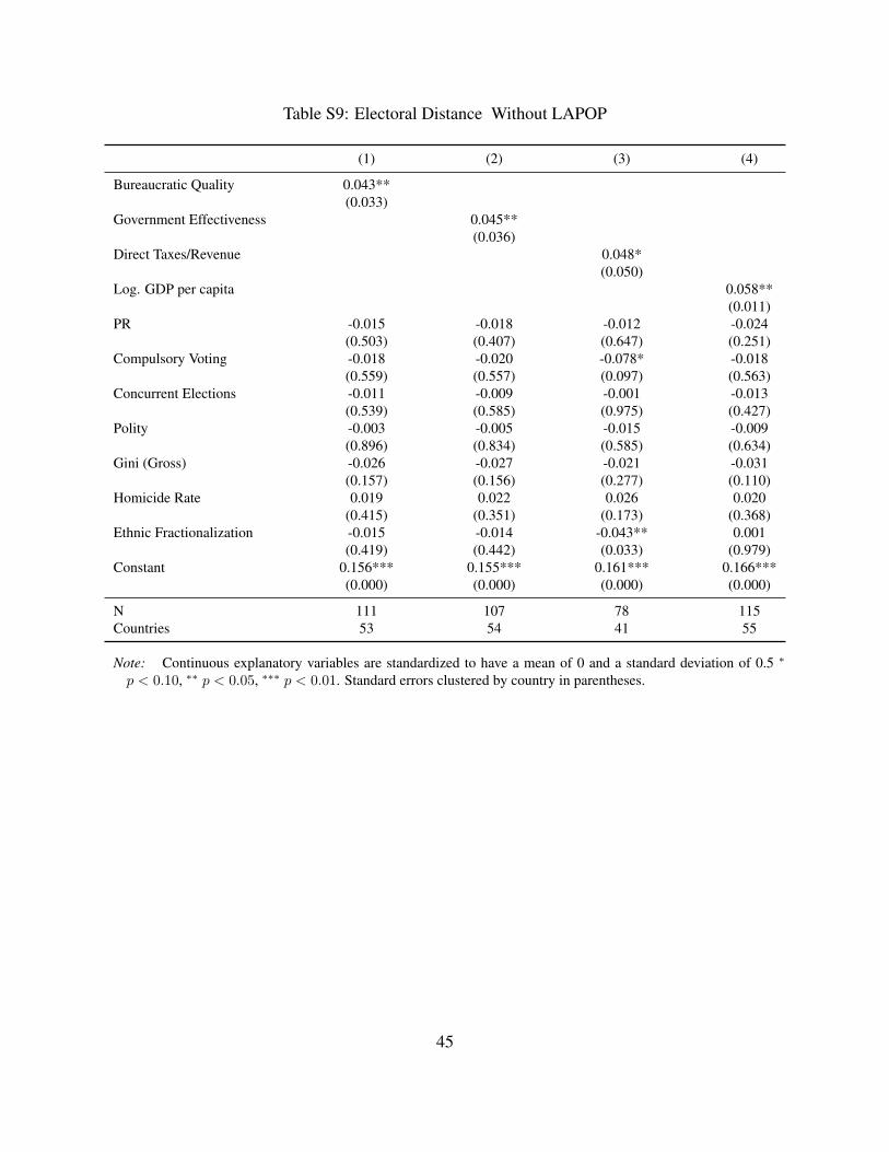
Table S9: Electoral Distance Without LAPOP

(1) (2) (3) (4)





PR -0.015 -0.018 -0.012 -0.024(0.503) (0.407) (0.647) (0.251)

Compulsory Voting -0.018 -0.020 -0.078* -0.018(0.559) (0.557) (0.097) (0.563)


Polity -0.003 -0.005 -0.015 -0.009(0.896) (0.834) (0.585) (0.634)

Gini (Gross) -0.026 -0.027 -0.021 -0.031(0.157) (0.156) (0.277) (0.110)

Homicide Rate 0.019 0.022 0.026 0.020(0.415) (0.351) (0.173) (0.368)

Ethnic Fractionalization -0.015 -0.014 -0.043** 0.001(0.419) (0.442) (0.033) (0.979)

Constant 0.156*** 0.155*** 0.161*** 0.166***(0.000) (0.000) (0.000) (0.000)

N 111 107 78 115Countries 53 54 41 55



45

Table S10: Electoral Distance Without Latinobarometer

(1) (2) (3) (4)





PR -0.029 -0.036** -0.017 -0.035*(0.139) (0.047) (0.439) (0.086)


Concurrent Elections -0.029* -0.026* -0.014 -0.030*(0.099) (0.083) (0.570) (0.061)

Polity -0.006 -0.016 -0.018 -0.005(0.741) (0.337) (0.496) (0.751)

Gini (Gross) -0.033** -0.032* -0.037* -0.036**(0.043) (0.064) (0.055) (0.031)

Homicide Rate 0.017 0.027 0.038** 0.016(0.404) (0.165) (0.025) (0.480)


Constant 0.155*** 0.157*** 0.159*** 0.162***(0.000) (0.000) (0.000) (0.000)

N 132 128 79 136Countries 58 59 41 60



46

Table S11: Electoral Distance Without WVS

(1) (2) (3) (4)





PR -0.023 -0.030 -0.012 -0.031(0.238) (0.114) (0.568) (0.143)



Polity -0.003 -0.014 -0.017 -0.003(0.840) (0.392) (0.510) (0.854)

Gini (Gross) -0.036* -0.030 -0.038* -0.039**(0.065) (0.137) (0.051) (0.030)

Homicide Rate 0.024 0.031 0.038** 0.022(0.251) (0.142) (0.030) (0.318)

Ethnic Fractionalization -0.011 -0.007 -0.035* -0.003(0.544) (0.688) (0.070) (0.851)

Constant 0.140*** 0.140*** 0.141*** 0.148***(0.000) (0.000) (0.000) (0.000)

N 144 140 79 148Countries 52 50 38 54



47

Table S12: U.S.:Electoral Distance – Controlling for Union Membership


Direct Tax/Revenue 0.108*** 0.114** 0.112** 0.146***(0.003) (0.019) (0.018) (0.007)

Tax/Revenue 0.105***(0.006)

Gini -0.010 -0.022 -0.035(0.844) (0.653) (0.512)

Between Group Inequality -0.129 -0.163*(0.112) (0.084)

% Union Membership (1939) 0.031 0.044 0.030 0.013 0.003(0.420) (0.268) (0.441) (0.736) (0.939)

Deep South -0.159** -0.140* -0.162** -0.136*(0.034) (0.070) (0.037) (0.079)

% Black -0.054 -0.064 -0.051 0.026 -0.051(0.441) (0.376) (0.477) (0.760) (0.687)

Constant 0.278*** 0.273*** 0.280*** 0.272*** 0.249***(0.000) (0.000) (0.000) (0.000) (0.000)

N 46 46 46 46 37



48

Table S13: U.S.:Voting Polarization


Direct Tax/Revenue 0.057** 0.061** 0.061** 0.077**(0.014) (0.025) (0.022) (0.011)

Tax/Revenue 0.048*(0.050)

Gini -0.010 -0.008 -0.006(0.751) (0.793) (0.864)

Between Group Inequality -0.078* -0.097*(0.090) (0.074)

Deep South -0.084** -0.079* -0.087** -0.067(0.043) (0.066) (0.043) (0.120)

% Black -0.042 -0.045 -0.038 0.006 -0.035(0.293) (0.275) (0.350) (0.895) (0.626)

% Manufacturing Employment 0.019 0.022 0.023 0.011 0.002(0.398) (0.363) (0.380) (0.688) (0.957)

Constant 0.158*** 0.157*** 0.159*** 0.153*** 0.140***(0.000) (0.000) (0.000) (0.000) (0.000)

N 46 46 46 46 37



49

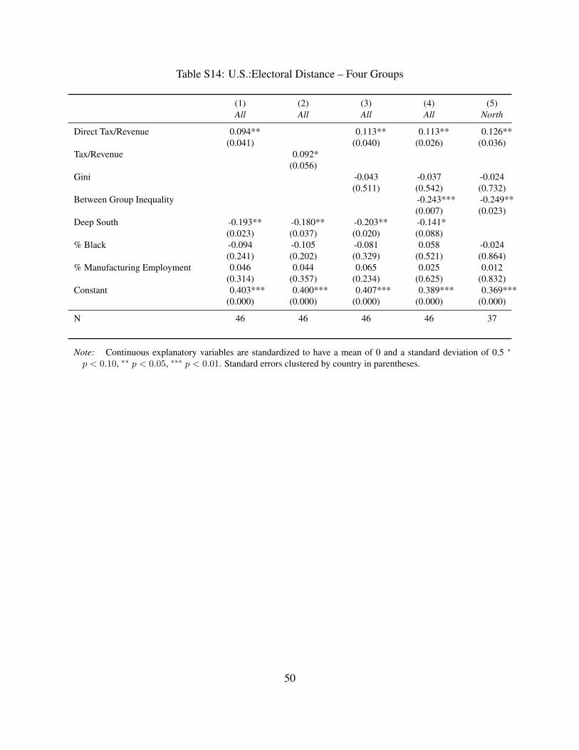
Table S14: U.S.:Electoral Distance – Four Groups


Direct Tax/Revenue 0.094** 0.113** 0.113** 0.126**(0.041) (0.040) (0.026) (0.036)

Tax/Revenue 0.092*(0.056)

Gini -0.043 -0.037 -0.024(0.511) (0.542) (0.732)

Between Group Inequality -0.243*** -0.249**(0.007) (0.023)

Deep South -0.193** -0.180** -0.203** -0.141*(0.023) (0.037) (0.020) (0.088)

% Black -0.094 -0.105 -0.081 0.058 -0.024(0.241) (0.202) (0.329) (0.521) (0.864)

% Manufacturing Employment 0.046 0.044 0.065 0.025 0.012(0.314) (0.357) (0.234) (0.625) (0.832)

Constant 0.403*** 0.400*** 0.407*** 0.389*** 0.369***(0.000) (0.000) (0.000) (0.000) (0.000)

N 46 46 46 46 37



50

Table S15: U.S.:Electoral Distance in Partisanship


Direct Tax/Revenue 0.078* 0.115** 0.116** 0.165**(0.085) (0.030) (0.031) (0.010)

Tax/Revenue 0.104**(0.025)

Gini -0.085 -0.085 -0.120(0.173) (0.177) (0.115)

Between Group Inequality -0.028 -0.043(0.755) (0.696)

Deep South -0.058 -0.040 -0.074 -0.068(0.466) (0.613) (0.354) (0.410)

% Black -0.111 -0.127* -0.096 -0.078 -0.065(0.117) (0.071) (0.175) (0.405) (0.667)

% Manufacturing Employment -0.032 -0.049 0.005 0.001 0.005(0.475) (0.283) (0.922) (0.989) (0.930)

Constant 0.286*** 0.281*** 0.290*** 0.289*** 0.289***(0.000) (0.000) (0.000) (0.000) (0.000)

N 47 47 47 47 37



51

Bureaucratic Capacity and Class Voting: Evidence from ...

Documents

Transcript of Bureaucratic Capacity and Class Voting: Evidence from ...