8MR PUBLICATIONS COMPACIUS ~ (LENDING SECTION)

BUREAU OF MINERAL RESOURCES, GEOLOGY AND GEOPHYSICS

RECORD

RECORD 1987/3

QUEST FOR THE MAGNETIC POLES: RELOCATION OF THE SOlITH MAGNETIC POLE AT SEA, 1986.

C.E. Barton. R. Hutchinson. P. Quilty. K. Seers and 1'. Stone.

The information contained in this report has been obtained by the Bureau of Mineral Resource., Geology and Geophysics as part of the policy of the Australian Government to assist in the exploration and development of mineral resources. It may not be I q 8 7 13hed in any form or u.ed in .. company prospectus or statement without the permis.ion in writing of the Director.

•

•

•

•

•

•

•

•

•

•

•

•

RI·:CORD 1987/3

QUEST FOR TilE MAGNETIC POLES: RELOCATION OF TilE SOlInl MAGNETIC POLE AT SEA, 1986.

o

C.E. Banon l, R. Hutchinson l , P. Quilty2, K. Seers1 and T. Stone1•

1 Bureau of Mineral Resources 2 Antarclic Division, Deparlmcnt of Scicnce. Kingston. Tasmania.

\

• \ I , \ "

1 !

.,

•

•

•

•

•

•

•

•

•

•

•

CONTENTS

Abstract

Introduction

Magnetic and Geomagnetic Poles

Movement of the Magnetic Poles

Discovery of the North Magnetic Pole

Discovery of the South Magnetic Pole

Location of SMP, January 1986

Compensation for the ships field

Observational technique

Results

Conclusion

Acknowledgements

References

Table 1 - Fluxgate alternator settings and calibration figures

Table 2 - Summary of SMP observation~

Appendix A

Appendix B

Appendix C

Figures:

Theory of the observational technique

Rate of change of dipole field at a magnetic pole

Program listing

1. Schematic of the magnetic and geomagnetic poles

1

1

1

2

3

4

7

9

9

11

13

14

14

9

12

15

17

18

of the earth 2

2. Diural paths' of the NMP and SMP in 1975 3

3. Roote to the SMP followed by TWE David and party, October 1908-January 1909. 5

4. David, Mawson and Mackay at SMP, 16 January 1909 6

5. Fluxgate sensor unit and Helmholtz coil assembly, stem of "Icebird" 8

6 .

7.

Horizontal intensity of magnetic field around southern dip pol~ epoch 1986.0

Rate of change of H with distance as a function of true bearing, epoch 1986.0

8. Observed position of SMP 2 - 3 January and 5 - 6 January, 1986.

9. Movement of SMP since 1600AD

iii

10

10

11

13

\ · \ I I

•

•

•

•

•

•

•

•

•

•

•

r\b~1ract

There is a rich and inLCresling hislory relating lo the exploralion for the South Magnelic Pole (SMP), in which Auslralians have played a leading role. The presenllocation of the South Magnelic Pole (SMP) in the Soulhern Ocean provides an opportunily lO deLCrmine ilS position well-removed from local (coastal) anomalies.

Al 03:24 hrs Universal Time (12:44 hrs local meridian time) on 6lh January 1986, the position of the SMP was calculated lO be latilude 65°19.0' S, longitude 139°18.2' E. Observations of the magnilude and direction of lhe hori7.0ntal inlCnsilY of the geomagnetic field were made from onboard the Australian Antarctic charlCr vessel/cebird which was 11.3 kIn from the pole when the above position was determined. NOl enough observations were made lO

calculaLC the mean position of the SMP, although il was eSlimaled lO be at approximately 65~O' S, l39°IO' E, i.e. about half a degrcc soulh of the dip pole for IGRF 1985 at epoch 1986.0. This places the pole offshore aboul 150 km north-northwest of the French Antarctic base of Dumont d'Urville, 2750 km from the South Geographic Pole and 1800 km from the South Geomagnelic Pole. The average drifl raLC of the SMP since 1841 is about 9 kIn/yr.

This is the fIrst time that the position of either of the magnetic poles has been deLCrmined directly (i.e. at close proximily) from a ship and the closest-ever observed approach to the SMP. The three previous direct determinations of the position of the SMP, made on the Antarctic icecap remoLC from local anomalies, were by Douglas Mawson in1909, Eric Webb in 1912 and Pierre Mayaud in1952. The SMP passed close to Dumont d'Urville when it migrated out lO sea 30 years ago.

Introduction

During the second half of the 19th century and the early part of the 20th century there was tremendous interest in terrestrial magnetism, due largely to its importance for navigation. The discovery of the magnetic poles was considered a target for exploration almost equal in importance to that of the geographic poles. Both magnetic poles were the object of a succession of major polar expeditions, and both were reached before their respective geographical counterparts:

Pole North Magnetic Pole North Geographic Pole South Magnetic Pole South Geographic Pole

Date 31 May 1831 6 Apr 1909

16 Jan 1909 14 Dec 1911

Leader James Clark Ross Robert Peary Edgeworth David, Douglas Mawson Roald Amundsen

A knowledge of the position of the magnetic poles is of practical value for chart production and navigation, whereas the secular and diurnal motions of the magnetic poles provide information about the nature of internal and external sources of the magnetic field. Australia has strong historical links with the exploration for the South Magnetic Pole.

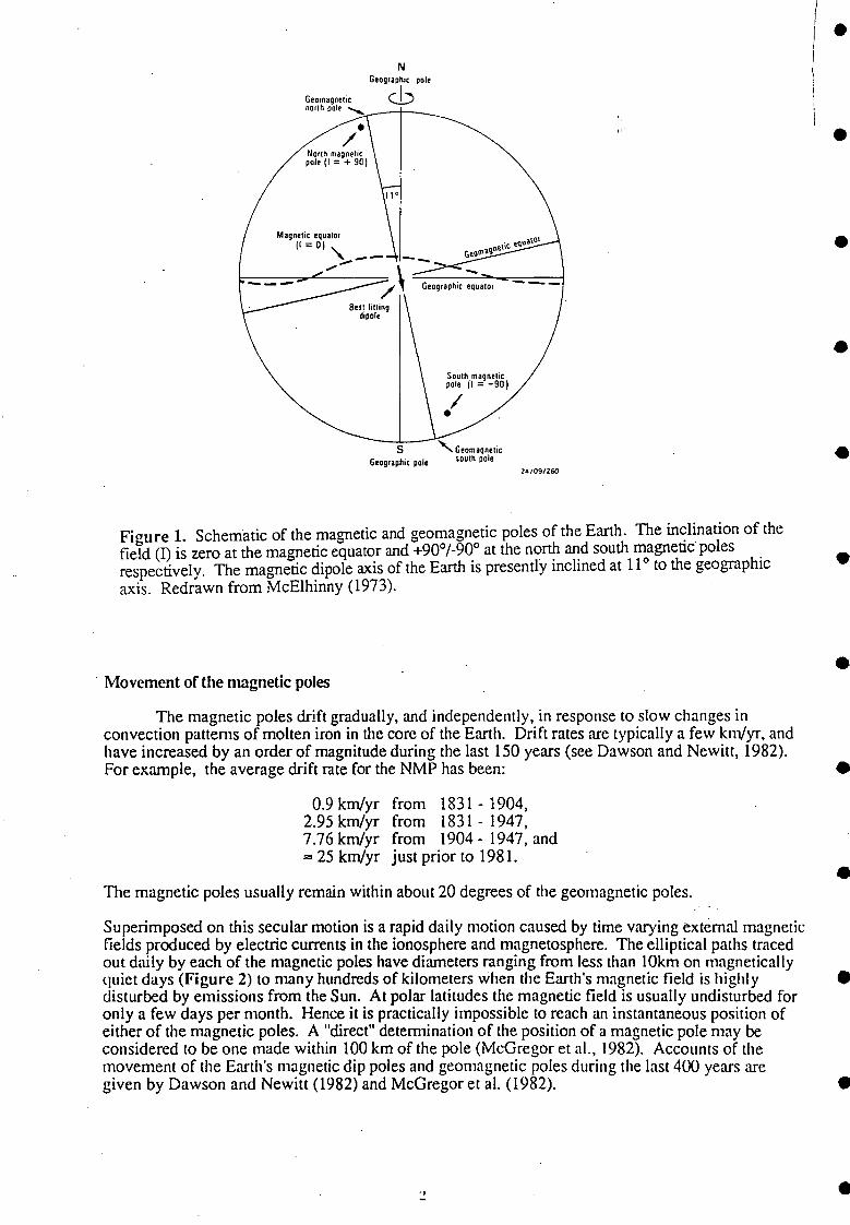
Magnetic and geomab'lletic poles

The magnetic poles, or dip poles as they are often called, are the principal points on the globe where the Earth's magnetic field points vertically upwards (the South Magnetic Pole, SMP), and vertically downwards (the North Magnetic Pole, NMP). The horizontal intensity of the geomagnetic field (H) at the magnetic poles is, of course, zero. This condition may also occur in the vicinity of intense localized magnetic field anomalies, but such cases are discounted ..

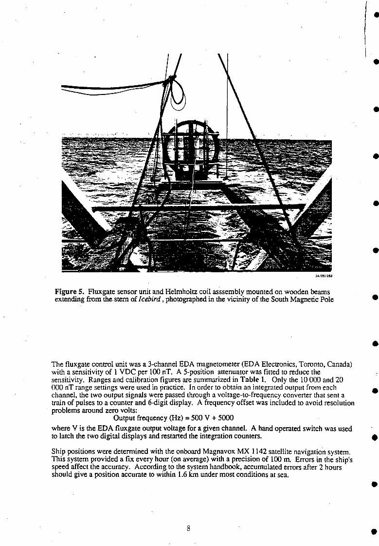
The north and south geomagnetic poles are determined by the intersection with the Earth's surface of the geocentric magnetic dipole axis of the Earth. These are antipodal by definition, and may be many thousands of kilometers from the NMP and SMP respectively (Figure 1). The geomagnetic poles are based on a mathematical concept, and are determined from a spherical harmonic analysis of observations of the geomagnetic field taken over the whole surface of the globe. The magnetic poles, on the other hand, have a physical manifestation - namely H = O. The geocentric coordinates of the South Geomagnetic Pole for epoch 1986.0, i.e. 1st January 1986, given by the International Geomagnetic Reference Field (IGRF, 1985 revision) are 79° 01.4' S, 109° 04.9' E, which is a distance of 1226 km from the South Geographic Pole. The corresponding location of the southern IGRF dip pole is 64° 43.3' S, 139° 10.0' E, which is 1859 km from the South Geomagnetic Pole and 2822 km from the South Geographic Pole.

Magnetic equator

N Geographic pole

cb

11=0) "-

,.. - - - \ =--~"""--=--I /

Best litting dipole

S Geographic pole

South magnetic pole 11=-90)

24/091260

Figure 1. Schemlltic of the magnetic and geomagn~tic poles of the Earth. The in~lination of the field (I) is zero at the ma~eti~ equat~r and +90o/-9~ at the no~ ~d south moagneuc poles . respectively. The magneuc dIpole axIS of the Earth IS presently InclIned at 11 to the geographIc axis. Redrawn from McElhinny (1973).

Movement of the magnetic poles

The magnetic poles drift gradually, and independently, in response to slow changes in convection patterns of molten iron in the core of the Earth. Drift rates are typically a few km/yr, and have increased by an order of magnitude during the last 150 years (see Dawson and Newitt, 1982).

•

•

•

•

•

•

•

For example, the average drift rate for the NMP has been: •

0.9 km/yr from 1831 - 1904, 2.95 km/yr from 1831 - 1947, 7.76 km/yr from 1904 - 1947, and == 25 km/yr just prior to 1981.

The magnetic poles usually remain within about 20 degrees of the geomagnetic poles.

Superimposed on this secular motion is a rapid daily motion caused by time varying external magnetic fields produced by electric currents in the ionosphere and magnetosphere. The elliptical paths traced out daily by each of the magnetic poles have diameters ranging from less than lOkm on magnetically quiet days (Figure 2) to many hundreds of kilometers when the Earth's magnetic field is highly disturbed by emissions from the Sun. At polar latitudes the magnetic field is usually undisturbed for only a few days per month. Hence it is practically impossible to reach an instantaneous position of either of the magnetic poles. A "direct" deternlination of the position of a magnetic pole may be considered to be one made within 100 km of the pole (McGregor et aI., 1982). Accounts of the movement of the Earth's magnetic dip poles and geomagnetic poles during the last 400 years are given by Dawson and Newill (1982) and McGregor et al. (1982).

.)

•

•

•

•

•

•

•

•

•

•

•

•

•

•

•

•

19 1"W 99"W 139°[ 1400[

65°30'S

8;_=-_ .. '-..4 N l-'/ \ 8~ " I} 12 I " . -.~6 20 24 \24 M/~~'.~ .• /

20

66°00'S

10 km I

66°30'S ,',;.

(a) 24/091261

Figure 2. Diurnal paths of (a) the NMP and (b) the SMP in 1975. Closed and open circles denote the average quiet-day paths and disturbed day paths respectively; stars shown the mean positions of the poles; numbers denote hours Universal Time; M & N shown local midnight and noon respectively. Redrawn from Dawson and Newitt (1982; figure 2)

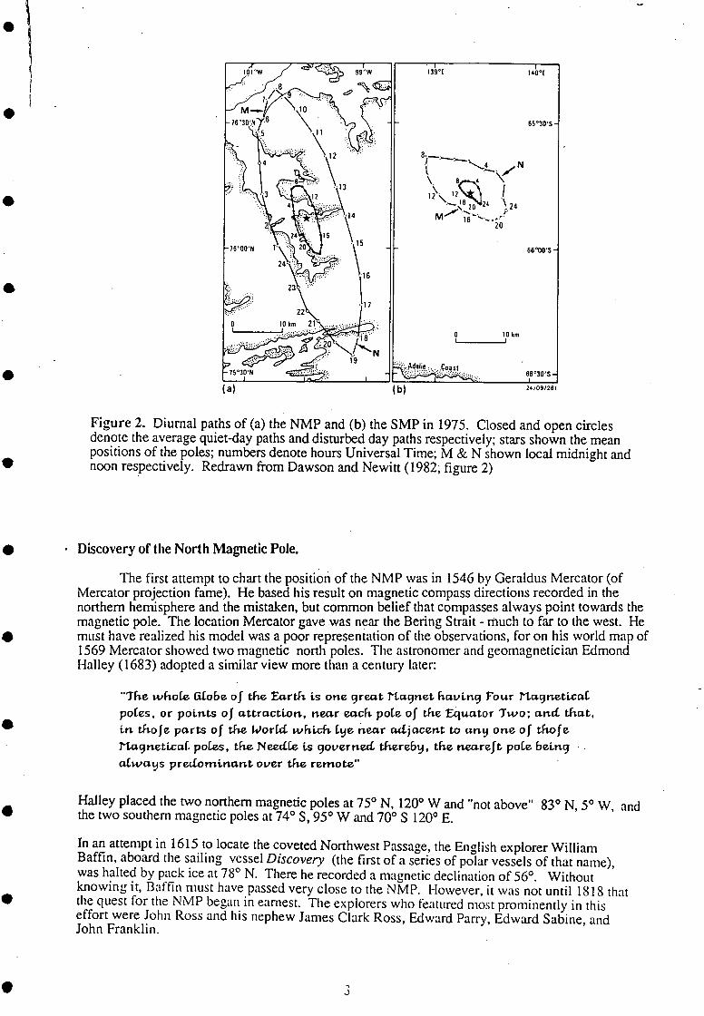
, Discovery of the North Magnetic Pole.

The first attempt to chart the position of the NMP was in 1546 by Geraldus Mercator (of Mercator projection fame). He based his result on magnetic compass directions recorded in the northern hemisphere and the mistaken, but common belief that compasses always point towards the magnetic pole. The location Mercator gave was near the Bering Strait - much to far to the west. He must have realized his model was a poor representation of the observations, for on his world map of 1569 Mercator showed two magnetic north poles. The astronomer and geomagnetician Edmond Halley (1683) adopted a similar view more than a century later:

"The whoCe GLooe 0 f the :Earth i-s one IJreat J'1.aIJnet havi.nIJ four J'1.aIJneticaL poCes, or poi-nts of attracti.on, near each poLe of the Equator Two; and. that, ion thole parts of the JiJortd. which Lye n.ear ad.jacent to anyone of thofe J'1.aIJnet.ica[ poLes, the Need.Ce i.s IJoverned. therwy, the neareft poLe oei.nlJ aLways pred.omi-nant over the remote"

Halley placed the two northern magnetic poles at 75° N, 120° W and "not above" 83° N, 5° W, and the two southern magnetic poles at 74° S, 95° W and 70° S 120° E.

In an attempt in 1615. t? locate the c?veted Northwest Passage, the English explorer William Baffin, aboard the salling vessel Discovery (the first of a series of polar vessels of that name), was halted by pack ice at 78° N. There he recorded a magnetic declination of 56°. Without knowing it, Baffin must have passed very close to the NMP. However, it was not until 1818 that the quest for the NMP began. in earnest. The explorers who featured most prominently in this effort were John Ross and hIS nephew James Clark Ross, Edward Parry, Edward Sabine, and John Franklin.

. James Clark Ross, who maintained a lifelong interest in terrestrial magnetism, was the first person to set foot at the NMP, and still holds the record for the highest inclination observation ever recorded near either magnetic pole (890 59'). The expedition was under the command of John Ross and sponsored by Felix Booth, a distillery magnate and Sheriff of the City of London. Ross' vessel Victory was handicapped by a monstrous steam engine, the first to be used for polar exploration, which had a maximum speed of 3 knots. As a consequence of their slow progress the expedition was trapped in the ice at 69 0 59' N in Felix Harbour on Boothia Peninsula for two successive winters. Ross calculated the approximate position of the NMP and set off with a sledge expedition along the southwest coast of Boothia Felix. On 31st May 1831 he reached the NMP at 70° 5.3' N, 96° 46' W. After remaining icebound for a third winter the expeditioners finally abandoned the Victory, and were subsequently rescued from Lancaster Sound four months later.

The second direct detem1ination of the position of the NMP was by the Norwegian, Roald Amundsen, during his 1903-1907 expedition that successfully located the coveted Northwest passage. Amundsen made an extended set of observations and operated a magnetic observatory on King William Island for 2 years. He was able to demonstrate that the daily motion of the pole was along an elliptical path, and gave the mean position of the NMP for 1904 as 70° 3~' N, 95° 3~' W. Since .1831 the pole had moved some 66 km at an average speed of 0.9 km/yr, which is more than an order of magnitude slower than today.

The position of the North Magnetic Pole is now monitored routinely by the Canadian Department of Energy Mines and Resources, Division of Seismology and Geomagnetism. Historical summaries of the search for the NMP are given by Serson (1981,1982).

Discovery of the South Magnetic Pole

Shortly after Ross' visit to the NMP the German physicist Carl Friedrich Gauss predicted that the SMP would be at 660 S, 1460 E. His prediction was based on results of the first spherical harmonic analysis of worldwide observations of the field. To polar explorers this provided an irresistible challenge, particularly as nobody had succeeded in reaching this region of the globe.

•

•

•

•

•

•

Expeditions to discover the SMP by the French explorer Jules Sebastian Cesar Dumont d'Urville • aboard the Astrolabe in 1840, and the American Lieutenant Charles Wilkes in1838-1840 were successful in exploring much of the coast of East Antarctica (Adelie Land and Wilkes Land). However, they were only able to establish that the SMP must be to the east of the position predicted by Gauss.

On 30th September 1839 James Clark Ross set out from London with two vessels, the Erebus and .• the Terror, on what was to be the last of the great polar sailing voyages. His object was to plant the flag he had taken to the NMP at the SMP. While in Hobart visiting Sir John Franklin, who had been appointed the Governor of Tasmania, Ross heard of the discoveries of Dumont d'Urviile and Wilkes and resolved to attempt to penetrate the pack ice further to the east. This proved to be remarkably successful and resulted in his discovery of the sea and island named after him (with its two volcanoes, Erebus and Terror named after the ships). He succeeded in penetrating further • south than any previous attempt, and opened up the approach used by Shackleton, Amundsen and Scott to the geographic pole. Ross found his passage to the magnetic pole barred by the Trans-Antarctic Mountain chain. His final observations from Ross Island (780 S, 1680 E) in 1841 indicated the SMP to be some 250 Ian to the west.

Interest in polar exploration waned until the start of the 20th century.· Expeditions by Robert F. '. Scott aboard the Discovery (1901-1904) and Erich von Drygalski aboard the Gauss (1901-1903) were no more successful than Ross in getting closer to the magnetic pole, but did make extensive measurements from Cape Adare down the western coast of the Ross Sea. [The Gauss was specially built for Drygalski's expedition under the sponsorship of Dr Alexander von Neumayer, who spent many years in Australia as Director of the Melbourne Observatory, and conducted the first detailed magnetic survey of the Colony of Victoria.] •

4 •

.\ I-i

I I •

•

•

•

•

•

•

•

•

•

•

The first, and successful overland attempt to reach the magnetic pole was in 1909 during Shackleton's British Antarctic Expedition, 1907-1909. The objectives of the expedition were to reach both the geographic and magnetic poles from their base at Cape Royds on Ross Island, and to explore the land to the east of the Ross Sea. The SMP party comprised Prof. Tannatt William Edgeworth David from Sydney University (leader, until he relinquished this role to Mawson in the final days of the journey), DOllglas Mawson from the University of Adelaide (cartographer and magnetic observer), and the Scotsman Alistaire Mackay (medical doctor). The party carried the following magnetic instruments:

one 3" two 2.5"

Cary compass-theodolite (for slln and declination obsevations) Brunton prismatic compasses (which performed excellently)

one one

6" Trough needle (to detennine declination) Lloyd-Creak Dip Circle (for detennining inclir.ation and total intensity)

158'

o lO '"

StatutI Milts

, , , , , , , '-( , ( . ' .. ,";

"~ ". v

0 u T It

o s s

D MOUlfTA ,,,$

155' 24109/262

Figure 3. Route to the South Magnetic Pole followed by T.W.E. David, D. Mawson and A.F. Mackay to the SMP, October 1908 - January 1909.

5

Shackleton had come anned with the first motor vehicle to be used in Antarctica, a 12-15 hp air-cooled New Arrol-Johnston. Despite some injuries inflicted on the SMP party in' their attempts to keep this beast mobile (Mackay sustained a broken wrist), it did manage to establish depots at 10 km and 15 km. Beyond that the party was obliged to man-haul their 2 tons of equipment on two sledges, named the 'Christmas Tree' and 'Plum Duff after their appearance and contents respectively. The weight of the sledges and the nature of the terrain required working in relays dragging a single sledge at a time. In this manner progress was limited to a mere 6.5 km/day under good conditions. They advanced 390 km northwards along the western coast of the Ross Sea to reach Relief Inlet, north of the Drygalski Ice Barrier on 12th December 1908 (Figure 3). The difficulties they encountered can be gauged from the 2 weeks taken to cross this 32 km wide ice tongue. Here they depoted the Christmas Tree sledge before heading across the mountains and inland to the 2000m plate~u. It was already clear that their chances of reaching the magnetic pole and returning to the coast .in time to be picked up by the Nimrod before the end of January were slender. .

On 15th January Mawson observed a dip of 890 45', and suggested waiting for the pole to drift towards the party. However, they agreed to force march the remaining 21 km the following day to Mawson's calculated mean position of the pole, and return 18 km. This was an undertaking of no mean daring considering the nature of the weather and the exhausted condition of the party. Their efforts were rewarded, and on 16th January 1909 at 3.30 pm the Union Jack was hoisted at the calculated mean position of the magnetic pole at 720 25' S, 1550 16' E (Figure 4), with the previously rehearsed proclamation by Prof. David: "I hereby take possession of this area now containing the Magnetic Pole for the British Empire". They managed to covered the 400 km return journey to Depot Inlet in 18 days, and by great good fortune on the following day, 4th February, were sighted and picked up by the Nimrod.

Thus the SMP was reached 3 months before Peary reached the North Geographic Pole, and 3 years to the day before Robert Falcon Scott was to arrive at the SOllth Geographic Pole, only to discover Amundsen's success four weeks before. David, Mawson and Mackay's epic 2000 km man-hauled sledge journey to the SMP remains one of the most remarkable feats of An tarctic exploration.

1.' ~.

~ t .

", """'-. :., ' ...... _dj .... • f

Figure 4. T.W.E. David, D. Mawson and A.F. Mackay at the South Magnetic Pole, 16 January 1909.

6

I • I I.

•

•

•

•

•

•

•

•

•

•

•

•

•

•

•

•

•

•

•

•

•

•

The second visit to the SMP was made in 1912 by Eric Nonnan Webb during Mawson's 1911-1914 Australasian Antarctic Expedition. Webb was a dedicated geomagnetician and made extensive observations of the field, both at the expedition's base on Cape Denison at Commonwealth Bay and during the sledge journey to the magnetic pole with Captain Robert Bage (officer in charge) and Captain Frank Hurley. The steepest inclination recorded by Webb was -890

43.3' on 21st December 1912, at the party's most southerly observation point (station 7). Webb estimated from his previous observations that the rate of change of inclination with distance towards the pole was 0.23 minutes of arc/km. Thus they were about 62 km from the SMP. Both Webb and Mawson fully appreciated that it was impossible to determine' accurately the mean position of the magnetic pole without making an extensive set of observations spanning many weeks. '

Webb analysed and published Mawson's results as well as his own (Webb and Chree, 1925). He pointed out that Mawson's final calculation of the position of the magnetic pole was based on incomplete sets of dip circle observations made during the final stage of the journey to the magnetic pole (a full set of observations is tedious, even under ideal conditions, and was impractical under the conditions'and time constraints that Mawson suffered). Based on estimated corrections to Mawson's data, Webb concluded that the magnetic pole must have been approximately 130 km northwest of the position reached by David, Mawson and Mackay.

No further effort was made to reach the SMP for the next 40 years, although Vestine et al. (1947) published a set of global maps of the geomagnetic field with SMP positions for 1922, 1932, 1942 and 1945. The last close approach to the SMP was in 1952 by Pierre-Noel Mayaud during the French Antarctic Expedition' to Adelie Land. Magnetic observations were made in the vicinity of base at Port Martin and at Cape Denison, Commonwealth Bay, and at stations a short distance inland on the plateau. Based on the new and previous observations, Mayaud (1953) estimated the position of the magnetic pole to be 68° 7' S, 143.0° E. The nearest station to the SMP was the one 10 km south of Cape Denison, at a distance of 116 km. Observations made at coastal stations are difficult to interpret directly because of the effects of local magnetic anomalies. For example, mean values of the field recorded at the magnetic observatory at Dumont d'Urville point to an apparent position of the SMP nearly 100 kIn to the east of its true . position. The mean position of the SMP passed close to Dumont d'Urville when it drifted off the continent 30 years ago (Figure 9b), and the instantaneous position of the SMP must have passed, through the station on many occasions during its transient daily motion. Observations made at sea and on thick ice on the Antarctic plateau are relatively isolated from the problem of local magnetic anomalies.

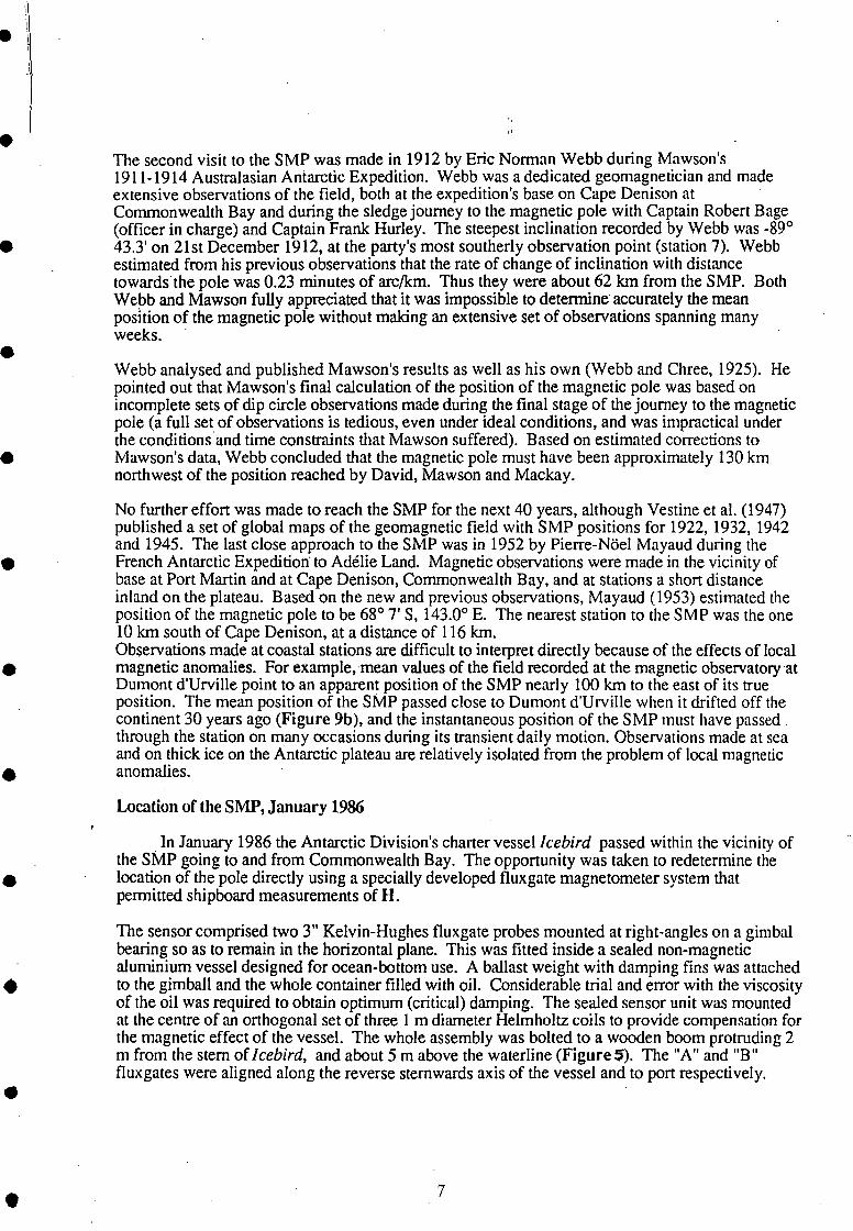
Location of the SMP, January 1986

, In January 1986 the Antarctic Division's charter vessellcebird passed within the vicinity of the SMP going to and from Commonwealth Bay. The opportunity was taken to redetermine the location of the pole directly using a specially developed fluxgate magnetometer system that permitted shipboard measurements of H.

The sensor comprised two 3" Kelvin-Hughes fluxgate probes mounted at right-angles on a gimbal bearing so as to remain in the horizontal plane. This was fitted inside a sealed non-magnetic aluminium vessel designed for ocean-bottom use. A ballast weight with damping fins was attached to the gimball and the whole container filled with oil. Considerable trial and error with the viscosity of the oil was required to obtain optimum (critical) damping. The sealed sensor unit was mounted at the centre of an orthogonal set of three 1 m diameter Helmholtz coils to provide compensation for the magnetic effect of the vessel. The whole assembly was boIted to a wooden boom protruding 2 m from the stem ofIcebird, and about 5 m above the waterline (FigureS). The "A" and "B" fluxgates were aligned along the reverse sternwards axis of the vessel and to port respectively .

7

24/09/2113

Figure 5. Fluxgate sensor unit and Helmholtz coil asssembly mounted on wooden beams extending from the, stern of Icebird, photographed in the vicinity of the South Magnetic Pole

The fluxgate control unit was a 3-channel EDA magnetometer (EDA Electronics, Toronto, Canada) with a sensitivity of 1 VDC per 100 nT. AS-position attenuator was fitted to reduce the sensitivity. Ranges and calibration figures are summarized in Table 1. Only the 10 000 and 20 000 nT range settings were used in practice. In order to obtain an integrated output from each channel, the two output signals were passed through a voltage-to-frequency converter that sent a train of pulses to a counter and 6-digit display. A frequency offset was included to avoid resolution problems around zero volts:

Output frequency (Hz) = 500 V + 5000

where V is the EDA fluxgate output voltage for a given channel. A hand operated switch was used to latch the two digital displays and restarted the integration counters.

Ship positions were detennined with the onboard Magnavox MX 1142 satellite navigatio'n system. This system provided a fix every hour (on average) with a precision of 100 m. Errors in the ship's speed affect the accuracy. According to the system handbook, accumulated errors after 2 hours should give a position accurate to within 1.6 km under most conditions at sea.

8

•

•

•

•

•

•

•

•

•

•

•

•

•

•

•

•

•

•

•

•

•

•

• r

Table I Fluxgate attenuator settings and calibration figures

Switch Nominal Calibration figure (nT/volt) position range (nT) Channel A Channel B

I ± 1000 102.3 102.6 2 ± 2000 200.0 201.0 3 ± 5000 487.3 490.0 4 ± 10000 959.4 959.4 5 ± 20000 1895.1 1918.8

Compensation for the ship's field

The Helmholtz coils, powered by separate constant current power supplies, were used to .provide first-order cancellation of the magnetic influence of the vessel. On the approach to the SMP (at 620 22' S, 141 0 54' Eon 01 Jan 86,20:12 UT) the currents in the Helmholtz coils were adjusted to null the field at the sensors with Icebird pointing along (B channel adjustment) and at right angles (A channel adjustment) to the magnetic meridian, as detemlined by the ship's magnetic· compass. Declination was 20° E at this point and the field of the vessel at the sensors in the forward direction was approximately 7000 nT. This simple compensation procedure turned out to be adequate, although better compensation could have been achieved by zeroing the averages of the appropriate sensor signals for the vessel pointing both forward and backwards along the meridian and transverse directions.

The magnetization induced in steel vessels by the Earth's magnetic field is commonly of the same order of magnitude as the permanent (remanent) magnetization, and must therefore be considered. In the vicinity of a magnetic pole the horizontal component of the geomagnetic field is small and we need concern ourselves only with induction by the vertical component. Because of the shape anisotropy of susceptibility of the ship, this will produce a horizontal field at the magnetometer. However, this will be virtually independent of the direction in which the ship is pointing and will effectively be a constant addition to the remanent magnetization component. Provided the cancellation procedure described above is perfornled close to the magnetic pole, no further correction is required. The observational technique used (below) was designed to give second­order cancellation of the magnetic effect of the ship.

Observational technique

Detenninations of H in the region of the pole were made by sailing the vessel in a tight circle at approximately constant angular speed. Signals from the A and B fluxgates (backwards and to port) were integrated over successive 20° sectors and converted to components along two fixed axes in space (X and Y) for each of the 18 sectors. When these components are averaged over a complete spin the residual field of the vessel cancels out and the magnitude and direction of II is obtained (Appendix A). Reduction of the sector size will improve the finite element approximations involved. It is convenient, but not necessary, for the reference axes X and Y to be geographic north and east.

For a purely dipolar field the rate of change of H with distance from the pole is 4.69 nT/Ion (for IGRF 1986.0), and the rate of change of inclination is 0.27 minutes of arc/krn (Appendix B). Direct observations of the rate of change of inclination with distance from the South Magnetic Pole were made byEric Webb in 1912, and integrated with the 1909 data and results from earlier indirect observations to obtain an isoclinic chart for the region (Webb and Chree, 1925; reproduced

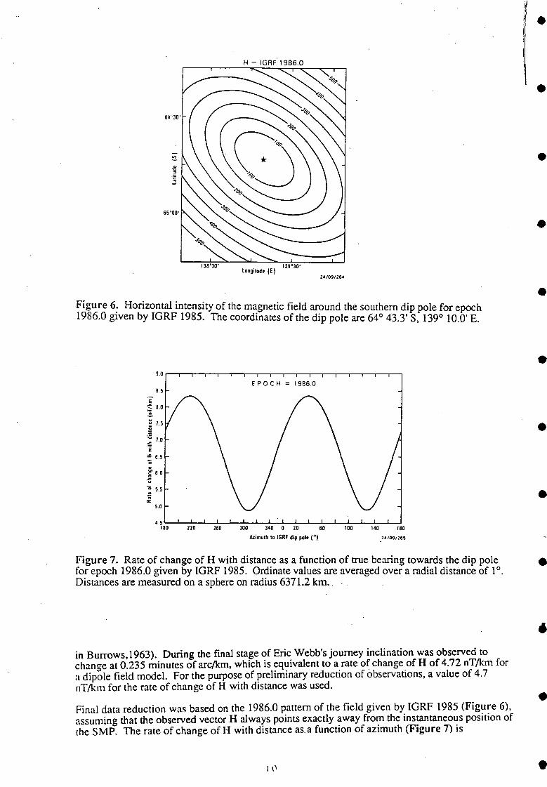
Figure 6: Horizontal intensity of the magnetic field around the southern dip pole for epoch 1986.0 gIven by IGRF 1985. The coordinates of the dip pole are 640 43.3' S, 1390 10.0' E.

8.5

~ 7.5

:a 70 = . i

:z: 6.5 o u f 6.0

~ 5.S

a:: 5.0

E poe H = 1986.0

4~8!;;0--L---:!22:;;-0 -1...--:2=60---..1.-=30:::-0 -1...-::3~40~0---!:20:---L--6Lo--L---l10-0 -L-1.L40--L--l180

Azimuth to IGRF dip pole (0) 24/09/285

•

•

•

•

•

•

•

•

Figure 7. Rate of ~hange of H with distan~e as a function of true bearing towards the dip pole • for epoch 1986.0 gIven by IGRF 1985. Ordmate values are averaged over a radial distance of 10. Distances are measured on a sphere on radius 6371.2 km.. .. .

in Burrows, 1963). During the final stage of Eric Webb's journey inclination was observed to change at 0.235 minutes of arc/km, which is equivalent to a rate of change of H of 4.72 nT/km for a dipole field model. For the purpose of preliminary reduction of observations, a value of 4.7 nT/km for the rate of change of H with distance was used.

Final data reduction was based on the 1986.0 pattern of the field given by IGRF 1985 (Figure 6), assuming that the observed vector H always points exactly away from the instantaneous position of the SMP. The rate of change of H with distance as.a function of azimuth (Figure 7) is

•

•

•

•

•

•

• en ° u.J Cl :=l l-t:: ex: ...J

•

•

•

•

•

•

•

•

65'00'

65'10'

65"20'

65'30'

- - - Pm" 2 ")lid 3 Jail

-- Path 5 and 5 Jan

<if---_. D"ection and distance to ship Ikmj

-tIn- Average speed (km/hr, .

348 ;14

2 Jan r:\ (09:51) \.!.)..

..... ..... ..... .....

.....

~ .....

.......... 260 ..... 11 ..... ,

" I ..,'" '%; 0)

(12:58) !:2'

5 Jan

(23:44)

0(02:06)

\

:., 74.6

~L 10 km

65'316j8':::.o':':'o'--------1--:'38~·30:':"' --------1-39~·0-:-0'---------:-13:-:':9·-:-30-' ---------:-14--'0·00'

LONGITUDE IOE) 24/09/266

Figure 8. Observed positions (circled numbers) of the South Magnetic Pole on 2-3rd January Goined by dashed line) and 5-6th January 1986 Goined by solid lines). Average speeds of the SMP between spins are shown boxed in the joining lines. Double arrows denote the direction a:nd distance to the ship when observations were made. Times of observations (UT) are shown in parenthesis beside each pole position. Observations 2/3 and 4/5 are averages of two consecutive spins.

considerably higher than for the dipole moo.el, and can be modelled to better than 3-figure accuracy by: .

dH = 6.7124 - .0184 Cos z + .0018 Sin z + .4196 Cos2z + 1.6611 Sin2z as _ .0073 Cos3z + .0142 Sin3z + .0980 Cos4z - .0528 Sin4z

+ .0022 Cos5z + .0004 Sin5z - .0098 Cos6z - .0107 Sin6z

where z is the azimuth relative to geographic north measured towards the dip pole. The actual pattern of the geomagnetic field in the region of the SMP has not changed substantially during this century (as noted by Vestine et al., 1947).

Results

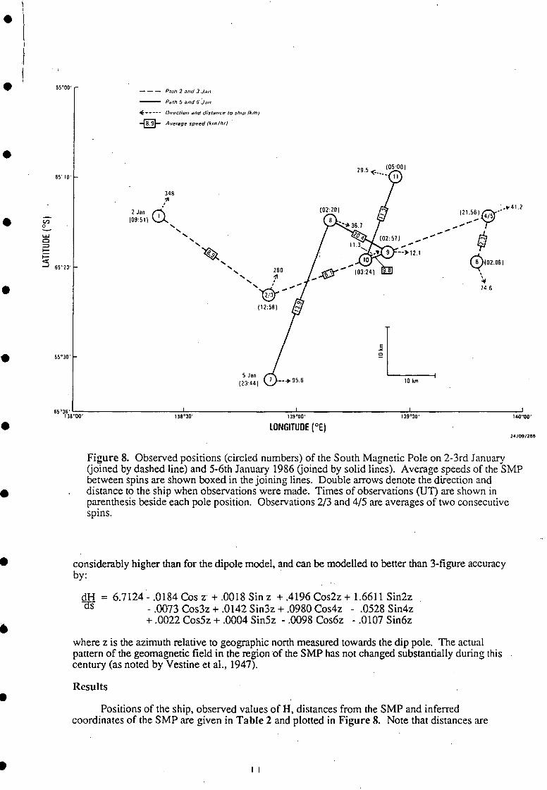
Positions of the ship, observed values of H, distances from the SMP and inferred coordinates of the SMP are given in Table 2 and plotted in Figure 8. Note that distances are

I I

...... N

•

TABLE 2.

SPIN UT UT SHIp·' s POSITION NO. DATE TIME LATITUDE LONGITUDE

(hr:min) (North) (East)

1 2 Jan 09:51 -62°30.0' 141°50.0'

2/3 2 Jan 12:58 -63°20;2' 141°28.6'

4/5 2 Jan 22:00 -65°05.9' 140°40.5'

6 3 Jan 02:06 -65°57.0' 140°21.9'

7 5 Jan 23:44 -65°36.0' 140°58.0'

8 6 Jan 02:20 -65°21.7' 139°54.0'

9 6 Jan 02:57 -65°18.3'· 139°39.7'

10 6 Jan 03:24 -65°16.7' 139°31.7'

11 6 Jan ·05 :00 -65°06.5' 138°49.0'

Results for consecutive pairs of spins

2 2 Jan 12: 54 -63°20.2' 141°28.6'

3 2 Jan 13:02 -63°20.2' 141°28.6'

4 2 Jan 21:52 -65°5.9' 140°40.5'

5 2 Jan 22:00 -65°5.9' 140°40.5'

• • • •

Summary of SMP observations

BEARING DISTANCE SMP POSTITION AV H TO SMP AWAY LATITUDE LONGITUDE MOVEMENT SPEED

(nT) (deg) (km) km km/hr

2864 207.5 348 -65°14.2' 138°23.0' 27.8 @ 8.9

2148 207.7 260 -65°23.1' 138°52.0' 48.9 @ 6.1

309 248.4 41.2 -65°14.0' 139°51.2' 9.8 @ 2.3

446 339.2 74 .6 -65°19.3' 139°47.6'

597 272.0 95.6 -65°32.6' 138° 53.0' 33.8 @ 13.9

202 285.7 36.7 _65° 15. 6' 139° 8· .9'

. 12.6 @ 20.~ . 76 271.6 12.1 -65°18. l' 139°24. l'

4.4 @ 9.8

86 247.2 11.3 -65° 19. 0' 139 ° 18. 2' 18.1. @ 11.3

168 102.3 29.5 -65° 9.8' 139°26.0'

2148 208.5 260 -65°22.1' 138°48.0' 3.8

2148 207.5 261 -65°23.8' 138°52~4'

249 244.9 32.2 -65°13.2' 140° 2.9' 18.2

370 252.0 49.9 -65°14.0' 139°39.4'

---.------

• • • • • • •

· \ I

•

•

•

•

•

•

•

•

•

•

•

I I

calculated for a spherical Earth of radius 6371.2 km (i.e. they are really a measure of the angle subtended at the centre of the Earth. Entries in the table for spins 2/3 and 4/5 are the means for these consecutive pairs of spins. Spin numbers 1,2 and 3 were made more than 200 km from the pole are not considered to be reliable, despite the excellent agreement between consecutive spins 2 and 3. The closest observed distance to the pole was 11.3 km for spin number 10 made at 03:24 hrs UT on 6th January 1986 (12:44 hrs ~ocal meridian time). Pole positions for the two pairs of spins differ by 3.8 km and 18.2 km respectively. This provides a measure of the uncertainty in the method. The effects of errors (particularly in the true bearing of the pole) become smaller as we approach the magnetic pole, and could be reduced substantially by averaging over many spins. There was not enough ship-time available to do this. '

A verage speeds of the S MP calculated between spins range from a few km/hr to a few tens of km/hr (Table 2). This is consistent with the moderate level of geomagnetic activity which prevailed on 2/3rd January and on 5/6th January 1986.

Conclusion

The position of the SMP has been detennined directly (i.e. from close proximity) by ship-board observations of the horizontal component of the Earth's magnetic field made on 2/3rd' January and 5/6th January 1986. The closest observed approach to the SMP was 11.3 km at 03:24 hrs UT, 6th January, when the magnetic pole was calculated to be at 65° 19.0' S, 139° 18.2' E.

Not enough observations were made during either of the two intervals of measurements to permit the mean position of the SMP to be calculated. However, the general sense and orientation of the pole path are consistent with that inferred indirectly by Dawson and Newitt (1982) from means of observatory data (Figure 2b). This suggests that the 'mean position of the magnetic pole is in the vicinity of 65° 20' S, 139° 10' E. The southern dip pole for IGRF 1985 at epoch 1986 is at 64° 43.3' S, 139° 10.0' E, i.e. about half a degree to the north. Successive southern dip pole positions for the IGRF (1985 revision) are shown on Figure 9b, and indicate that the pole drifted off the continent between Dumont d'Urville and Port Martin in about 1957.

135'

SOUTH POLE 241091267

IS'

ISS

0- 156

~ ~

~

~ 151

ISB

1990

1985

1980

1975

* Estimated mean position based on observations. Jan 1986

1945

15913~B ---'----:"'I'~O --'--:-'14-=-2 --'---:-'14-' ....J...-:-'146

Langilude (OE I 26/09/268

Figure 9. (a) Movement of the South Magnetic Pole since 1600 A.D. Asterisks denote direct detenninations, as defined in the text (including Ross' position for 1841); solid circles denote determinations based on charts and extrapolation from remote observations; the thick line is the SMP path given by the IGRF model, as detailed in (b). [Part (a) modified from McGregor et aI., 1982].

I .~

This is the first time that either of the magnetic poles has been located directly from onboard a ship. If we take Webb's corrections to Mawson's observations in 1912 (Webb and Chree, 1925), then this is also the closest observed approach to the SMP. Previous "direct" detenninations of the position of the SMP were made by Mawson in 1909, Webb in 1912 and Mayaud in 1952.

Movement of the SMP since 1600 A.D. is illustrated in Figure 9. Direct determinations (asterisks - including that of James Clark Ross in 1841) are combined with positions determined from remote observations and charts (solid circles) and the IGRF (open circles and inset). Since 1841 the SMP has drifted 1300 km in a north-northwesterly direction at an average speed of about 9 km/yr. Since 1952 its average drift rate has been about 10 km/yr. It is currently approximately 154 km offshore from the French Antarctic base of Dumont d'Urville in a north-northwesterly direction, 2750 km from the south geographic pole, and 1800 km from the South Geomagnetic Pole.

e.F. Gauss would be pleased to know that his prediction of the position of the SMP made in the 1930's is now in error by less than 300 km.

Acknowledgements

We thank the Captain and crew of lcebird for their cooperation and the Antarctic Division for logistic suppport. A. White loaned ocean-bottom magnetometer components, P.A. Hopgood calibrated the fluxgates, J. Bitterly and J. Folques, Institut de Physique du Globe, Strasbourg provided data from Dumont d'Urville, and P.L. McFadden generated ~he hannonic model of the IGRF dHlds curve. This paper is published with the permission of the Director, Bureau of Mineral Resources, Geology and Geophysics. . .

REFERENCES

Burrows, A.L. (1963), Location of the South Magnetic Pole. NZ. J. Geol. Geophys., 6& 454-464.

David, M.E. (1937), Professor David, the life of Sir Edgeworth David. Edward Amold,London Dawson, E. and L.R. Newitt (1982), The magnetic poles of the Earth. J. Geomag. Geoelectr.,

34, 225-240. Halley E. (1683). A theory of the variation of the magnetical compass. Phil. Trans. R. Soc.

London, 12, 208-221. IAGA Division I Working Group 1 (1985), International Geomagnetic Reference Field revision

1985. J.Geomag. Geoelectr., 35, 1157-1163. McElhinny, M.W. (1973), Palaeomagnetism and Plate Tectonics. Camb.Univ. Press,

Cambridge, pp.358. McGregor, P.M., A.J. McEwin and lC. Dooley (1982), Secular motion of the South Magnetic

Pole. In: R.L. Oliver, P.R. James and J.B. Jago (eds.), Antarctic Earth Science, Australian Academy of Sciences, Canberra, 603-606.

Mayaud, P.-N. (1953), Rapports scientifiques des expeditions pol aires Francaises S IV 2. Annales Geophys., 9, 266-276.

Ross, J.e. (1847), A voyage of discovery and research in·the Southern and Antarctic regions during the years 1839-43, John Murray, London.

Serson, P. (1981), Tracking the north magnetic pole. New Scientist, 90,616-618. Serson, P. (1982), The search for the North Magnetic Pole. Trans. Roy. Soc. Canada, 20.

391-398. Vestine, E.H., L. laPorte, I. Lange, C. Cooper, and W.C. Hendrix (1947), Description of the

Earth's main magnetic field, 1905-1945. Dept. Terrestrial Magnetism, Carnegie Institution of Washington Publication, No. 578.

Webb, E. N. and Cree, C. (1925), Scientific Reports, Australasian Antarctic Expedition 1911-1914, Series B, Vol. 1, Terrestrial Magnetism, p.55.

14

I I-I I. •

-•

•

•

•

•

•

•

•

.i •

•

•

•

•

•

•

•

•

•

•

APPENDIX A - Theory of the observational technique.

Let X, Y = arbitrary horizontal axes in space (geographic north and east are convenient)

A, B = stern-wards and port axes of the ship Hx Hy = horizontal components of the field along the X and Y axes ,

B = size of each integration section (degrees), e.g. 10° or 20° NAt NB = sum of the counts of the A and B channel integrators

x A Consider the ship spinning about a vertical axis at constant angular speed We divide each spin into an even number of small sectors, of size B (typically 10° or 20° in practice). Let 0 i be the angle between the X and A axes for the middle of the ith sector of the spin, and let the first sector start at 0=0 and time t=O (see sketch opposite).

B

Then y

0· = (i-I) 8 + 8/2 = 8 (i - 1/2) 1

........... (1)

As discussed in the text, the output of the voltage-frequency converter (in Hz) for a particular channel is given by

fout = 500 V + 5000 = 500 H/k + 5000

where V is the output voltage of the EDA fluxgate, k is the calibration figure in nTlvolt (see Table 1), and H is the field along the axis of the fluxgate. The mean value of the frequency for time interval t during which the counter accumulates N pulses is NIt.

Hence for the ith sector, the mean values of H in nT for the A and B channels are given by

HAi = (NA/~ - 5000) I 500 k

HBi = (NB/ti - 5000) I 500 k

These have components along the X and Y axes given by

x. = HAl' Cos 0· - HB· Sin 0· 1· 1 1 1

and Yi = HAi Sin 0 i + HBi Cos 0 i

........... (2)

........... (3)

However, if SA and SB are the components of the magnetic field of the ship along the A and B

axes, and ~ and Hy are the horizontal components of the Earth's field along the X and Y axes, then to a first approximation for small sector sizes (8),

x. = H + SA Cos 0· - SB Sin 0· 1 XII .......... (4) and Yi = Hy + SA Sin 0 i + SB Cos 0 i

S A and SB are constant, so when summed over one complete spin of the vessel comprising an even

number of sectors (n=360/B), the Sin and Cos terms become zero.

15

Hence Hx = 1 Li (Xi) = 1 Li ( HAi Cos 0i - HBi Sin 0i ) n n

and Hy = 1 Li (Yi) = 1 Li (HAi Sin 0i + HBi Cos 0i ) n n

Finally, the horizontal component of the Earth's field is of magnitude HE = ~(HX2 + Hi) at angle Tan- 1(Hy/Hx) clockwise from the X axis.

lntegrating the signals over fmite sectors introduces approximations into equations (3) and (4), but these is not important provided the sectors are fairly small, e.g. 10° or 20°. By extending the· integration over a finite number of spins (N) the signal-to-noise ratio can be improved by a factor of ~N.

Computer programs SMP85 and MAGPOLE, written in Microsoft BASIC 2.1 for an Apple Macintosh, are listed below. Program SMP85 performs the above calculations to find HE ' the true bearing of the pole and the distance to the pole in km (for a 1986.0 IGRF field model). Program MAG POLE computes magnetic pole coordinates from ship coordinates and the distance and true bearing of the magnetic pole. All coordinates are geocentric and all distances are measured on a sphere of radius 6371.2 km.

16

1.

I • •

•

•

•

•

•

•

•

•

•

• j

•

•

•

•

•

•

•

•

•

•

•

APPENDIX B - Rate of change of dipole field at a magnetic pole - -

Consider a point P at radial distance r and angle ~

(arc length, s) from a dipole of moment M as

sketched opposite.

The magnetic potential at P due to M is

U = r g~ Cos 0 ........ (1)

and gO = Ilo M I --

41t r3

¢

p

in SI units where Ilo = 41t 10-7 HIm, and g~ is the spherical harmonic Gauss coefficient

representing the axial dipole contribution to the magnetic potential. The tangential component of

the field is given by the appropriate partial derivative of U, namely

H = - au = - Qll . ~ = _.1. Qll = g~ Sin 0 . . . . . . . .. (2)

as a0 as r a0

thus dH = dH. ~ = g~ Cos 0 .......... (3)

ds d0 ds r

At the geomagnetic poles, Cos 0 = ±1, the geocentric radius is 6371.2 km, and g~ = 29855 nT for

1GRF 1986.0. Thus the rate of change of the horizontal component of the dipole field With great

circle distance is ±4.69 nT/km.

From radial and tangential derivatives of equation (1) it follows that the dipole field at a

geomagnetic pole (Fp) is twice that at the dipole equator, and the latter is equal to g~ . Furthermore,

the rate of change with distance of Fp is equal to (g~ Sin 0)/r and is therefore zero at each magnetic

pole, hence

and,

dI=l dH Fp

dI = dI. dH = 1 . g~ = 1 ds dH ds Fp r 2r

Hence the rate of change of magnetic inclination (dip) with distance from a geomagnetic pole is

1/12742 radians/km, i.e. 0.27 minutes of arc/km.

17

APPENDIX C. Program listings

'Prograrn SI"IP85 Ivlaci ntosh liS BAS I C 2, I Rev: 09 Dec 86 'Does 2-a:--;is sector summation for SI"IP project, using 1985 calibration Ijeta 'Input:

8 - sector size (Ijeq) Ka(5), Kb(5) - sensitivit.~d of A, B channels for each switch setting (nT IV) AZ - true bearing of starting, X-axis (deg) NA, N8 - readings for the A and 8 channel integration counters TS - time interval for each sector (sec)

'Output: H - horizont.al component of Earth's fie\lj (nT) Hx, Hy - fields along :~ and 'Y exes (nT) S8, Sb - residuel field of ship along ~\ end B exes (nT) DD - true bearing to pole (deg) RATE - IjH/ds (nT Ikrn) from harmonic model of IGRF85 at epoch 1986.0

, 1<1"1 - distance t.o pole in km on sphere of redius 6371.2 km

CLS WIDTH 72,9

I<e( 1)= I 02.3 :l<a(2)=200! :l<a(3)=4i37.3 :l<a(4)=959.4 :l<a(5)= 1895.1 Ktl( 1)= 102.6 :I<:b(2)=20 I! J::t.(3) = 490! :!<tI(4)=959.4 :l<b(5)= 1916.8 PRINT: LPRINT

200 PR I NT" --------------------Progr81n SIvlP85 --------------------":PR I NT

RATO=6.7124 :'rneandH/ds over I,jeg from SI"IP for IGRFI986 in nT/krn AZ=O :'default true bearing(T.B.) of starting axis

300 INPUT" Se.ctor size (deg): ";8 :'Reset pararnet.er~; LPRINT" Sector 5ize=".:8;" deg" NS=360lB I :'nurntler of sect.ors per ~;pin INPUT" Attenuator S"NitCI'! position( 1-5)= ";SVl PRINT" Sensitivity fact.or for channel A (nT/V): :~;Ka(SVn PRINT" Sensitivitld factor for channel Ei (nT/V)= ";Kb(Sv.J) lPRINT" ::;en::iif.ivif.y factor for channEd A (nT 1'1)= ";Ka(SV-/) LPRINT" Sensitivity foctor for channel B (nT/V)= ";Kb(SI,"i) INPUT" Reconj (~,pin) number= ";NUI"I r'·JUI"l=NUI"I-l

320 NUI'I=NUI"l+ I : PRINT: lPRINT :'start next spin PRINT" Record (spin) nl.lmber";NUI"1 lPRINT" Record (spin) nurnber"}JUl"1 : LPRINT INPUT" True bearing (deg) of origin exis (O=no change)="; AZZ IF(AZZoO) THEN AZ=AZZ LPRINT" True bearing of origin axis = ";AZ : LPRINT

SUMX=O:SUMY=O:SUMA=O:SUMB=O FOR 1= I TO NS

BEEP: PRINT: PRINT" Sector number";1 350 INPUT" A counter="; NA

18

•

•

•

•

•

•

•

•

•

•

•

•

· \ • I

•

•

•

•

•

•

INPUT" B, counter="; NB 3 -0 INPUT" C' t t· ( '\" T("' b ·...Iee .or lme~sec.,;::; .J

IF(TS=O) THEN 360 INPUT" Continue (any key), repeat la~;t entry (R)";Q$ IF(O.$="R" OR Q$="r") THEN 350

HA=(NA!(TS*500)-1 O)*l<a(Sv.;) : HB=(N6!(TS*500)-1 O)*l<tl(~;It,1) A=RPD*B*( 1-.5) 5UMA=SUMA+HA:SUMB=SUMB+HB SUMX=SUlvl:~ + HA*C05(A) - HB*5IN(A) ~;LWJII=5UI"1V + HA*5IN(A) + HB*C05(A)

NEXT BEEP: BEEP HX=SUI"IX/NS : HY=SUI"IY INS SA=SUt'IA/NS : S6=SUlvlB/NS H=5QR(HX*H:~ +HV*HV)

:'H compts~ a long chosen axes :'Ship's field

D=DPR* A TN(H'UHX) : I F(HX<O) THEN D=D+ 1 CiO :'Re 1. azi mutl) of H DD=D-180+AZ: DR=DD*RPD :'True bearin'~ to pole

RA TE=r:;~ATO-.O 184*C05(DR)+.OO 1 Ci*51 N([iR)+.4196*C05(2*DR)+ 1.6611 *51 N(2*DR) RATE=RATE - .0073,*C05(::::,*Dr:;~)+.O 142*5 I N(3*DR)+.098*C05(4*DR)-.0528*5 I N(4*DR) RATE=F-~ATE + .0022*C05(5*DR)+ .0004*5 I N(5*DR)- .0098*C05(6*Dj:;~)-.0 1 07*5 I N(6*DR) krn=HlRATE

H:~=.I*INT(10*Hl;+.5): H't':.1*INT(10*HV+.5) :'rounlj ior printing SA=.1 *INT( 1 O*SA+.5) : SB=.1 *INT( 10*S6+.5) H =.1*INT(10*H+.5): DD=.Ol*INT(lOO*DD+.S) RATE=.OO 1 * I NT( 1 OOO*RATE + .5) : km=. 1 * I NT( 1 O*krn+ .5) PRINT PRINT" H:"~=";H:~:;" Hy=".:H'(" Sa=";SA;" Sb=";SB.:" nT" PRINT" H=";H;"nT, T.B. to pole=".;DD;",jeg, Rate=";RATE.;"nT/km, Dist=".;km;"km" PRINT:lPRINT lPRINT" H:~=";H:~.;" HV=";HV;" SA=";SA;".· 5B=";S8.;" nT" lPRINT" H=";H.;"nT, T.B. to pole=";DD;"deg, F.~ate=";RATE;"nT/km, Dist=".:krn;"krn" lPRINT

• 900 INPUT" Next spin (1-,0., Reset parameters (R), Quit (Q)".: Q$ PRINT: lPRINT IF(Q$="n" OR Q$="N") THEN 320 :'next spill., sarne parameters IF(Q$="r" OR Q$="R") THEN 300 :'reset parameters IF(Q$="Q" OR Q$="Q") THEN 999 :'Quit

• GOTO 900 999 END

•

19 •

:rvlAGPOlE r"lacintosl1 r1S BASIC 2.1 Rev: 3 Dec 86 'I nput: ~31)i p lat..(N) .. lon.(£), di sf.. to po 1 e (km), true beari ng to po 1 e (E) 'Output: Pole lat u·n., Ion (E) i~ deg and ,jeg+rnins 'Uses geocentric coordinates .. Eartl) raditls=6371.2 km 'Enter angles as +/- deg an,j mins (rnins always positive)

CLS WIDTH 72,9 DfFSNG A-Z DfF FNASN(X)=ATN(X/SQR( -X*X+ 1)) DfF FNACS(~:)= 1.570796#-ATN(X!SQR( l-X*X) DPR=:45/ A TN( 1): RPD= I!DPR

200 PRINT:PRINT" --------------- Program MAGPOlE ---------------":PRINT

INPUT" ~3hip let (N) degrees="; SL T INPUT" - - - - - - - minutes="; SLTrt IF(SLT<O) THEN SlTr1=-SLTr-l SL T =SL T +SL Trv1/60 I NPUT" ~=;t'1i P long (E) degrees=".: SLN INPUT" - - - - - - - minutes=",: sum: IF(SUhO) THEN ~3LNr"1=-SLNr-l SLN=SLN+~3LNI"1/60

INPUT" True beerinQ to pole (,jeqE) ="; DD ~ ~

INPUT" Di~;t8n(:e to tn8gpole (krn) ="; :~D D=DD*R.PD : S=(90-SL T)*RPD : :~=W/6371.2 :' ~3=(:o lat" X= di sf.. in red.

P=FNACS(COS(S)*COS(X)+SIN(S)*SIN(:~)*COS(D» :' pole colet in rad A=FNASN(SIN(D)*SINC~)/SIN(P)) :' polar angle of spt1.triangle PL T =90-(P*DPR) : PLN=~3LN+(A*DPR) :' rnel,~pole lot, Ion

PL TD= I NT(Pl T) : PL Tr1=(Pl T -PL TD)*60 I F(PL TD<O) THEN PL TD=PL TD+ 1 : PL TI"1=60-PL TI"l PLND= I NT(~LN) : PLNfYl=(PLN-PLND)*60 IF(PLND<O) THEN PLND=PLND+ 1 : PLNI1=60-PLNM

PRINT: LPRINT PRINT" r-lagpole latitude (1'1) = ";PLT;"deg PRINT" 1'1agpole longitude (E)= ";PLN;"deg lPRINT" Ship lat=";SLT.:" lon=";SLN;" ,jeg lPR I NT" r1agpole latitude (N) = ";PLT;",jeg lPRINT" Magpole longitude (E)= ";PLN;"deg PRINT: lPRINT

INPUT" Repeat (RETURN) or Quit (0)";0$

IF(Q$="q" OR 0$="0") THEN END PRINT: ClS :' clear screen

=";PL TD;",jeg ";PL TI"l;"min" =";PLND;"deg ";PLNl"l;"min"

Azim=";DD;" deg Dist=";XD;" km" =";PLTD;"deg ";PL Tr1;"min" =";PLND;",jeg ".:PLNM;"min"

,SL Tr-l=O: SLNr1=O: Dry l=O :' clear mins to allow return default=O GOTO 200 :' return for next record

999 END

•

•

•

•

•

•

•

•

•

•