Buoyancy-dominated displacement ﬂows in near-horizontal ...

J. Fluid Mech. (2009), vol. 639, pp. 1–35. c© Cambridge University Press 2009

doi:10.1017/S0022112009990620

1

Buoyancy-dominated displacement flowsin near-horizontal channels: the viscous limit

S. M. TAGHAVI1, T. SEON2, D. M. MARTINEZ1

AND I. A. FRIGAARD2,3†1Department of Chemical and Biological Engineering, University of British Columbia, 2360 East Mall,

Vancouver, BC, Canada V6T 1Z32Department of Mathematics, University of British Columbia, 1984 Mathematics Road,

Vancouver, BC, Canada V6T 1Z23Department of Mechanical Engineering, University of British Columbia, 6250 Applied Science Lane,

Vancouver, BC, Canada V6T 1Z4

(Received 31 December 2008; revised 25 May 2009; accepted 26 May 2009; first published online

16 October 2009)

We consider the viscous limit of a plane channel miscible displacement flow of twogeneralized Newtonian fluids when buoyancy is significant. The channel is inclinedclose to horizontal. A lubrication/thin-film approximation is used to simplify thegoverning equations and a semi-analytical solution is found for the flux functions. Weshow that there are no steady travelling wave solutions to the interface propagationequation. At short times the diffusive effects of the interface slope are dominantand there is a flow reversal, relative to the mean flow. We are able to find a short-time similarity solution governing this initial counter-current flow. At longer timesthe solution behaviour can be predicted from the associated hyperbolic problem(where diffusive effects are set to zero). Each solution consists of a number N � 1of steadily propagating fronts of differing speeds, joined together by segments ofinterface that are stretched between the fronts. Diffusive effects are always presentin the propagating fronts. We explore the effects of viscosity ratio, inclinations andother rheological properties on the front height and front velocity. Depending onthe competition of viscosity, buoyancy and other rheological effects, it is possible tohave single or multiple fronts. More efficient displacements are generally obtainedwith a more viscous displacing fluid and modest improvements may also be gainedwith slight positive inclination in the direction of the density difference. Fluids thatare considerably shear-thinning may be displaced at high efficiencies by more viscousfluids. Generally, a yield stress in the displacing fluid increases the displacementefficiency and yield stress in the displaced fluid decreases the displacement efficiency,eventually leading to completely static residual wall layers of displaced fluid. Themaximal layer thickness of these static layers can be directly computed from a one-dimensional momentum balance and indicates the thickness of static layer found atlong times.

1. IntroductionIn this paper we consider miscible displacement flows along a plane channel of

width D in the large Peclet number limit Pe � 1 (where Pe = DU0/Dm, with U0

† Email address for correspondence: [email protected]

2 S. M. Taghavi, T. Seon, D. M. Martinez and I. A. Frigaard

the mean displacement velocity and Dm the molecular diffusivity). In this limit, inthe absence of any flow instability, the fluids have insufficient time to mix on timescales of experimental interest and a reasonable approximation is to model the twofluids via a kinematic equation, rather than a concentration-diffusion-equation (CDE)approach. The stability of the flow cannot generally be determined beforehand andoften the reason for this type of model simplification is to make study of the stabilityproblem possible, as well as to gain basic understanding of the laminar flow. Thescenarios that we consider involve fluids of different densities, with Newtonian ornon-Newtonian shear rheology.

Within the class of large Peclet number displacement flows, we consider those inwhich buoyancy is a significant force in driving the fluid motion and restrict our studyto those in which the channel is approximately horizontal. In the absence of a meanflow (U0 = 0), the only driving force would be buoyancy. For sufficiently small densitydifferences there exists a viscous regime in which inertial effects are small and forwhich the interface slumps under gravity and elongates along the channel. If now amean displacement flow is introduced, we may expect that the viscous regime persistsfor at least small Reynolds numbers Re (= ρU0D/μ). Indeed, when the flow topologyevolves into an elongated slumping interface with near-parallel streamlines, of aspectratio δ � 1, inertial effects remain negligible provided that δRe � 1. This allows fora more practical range of Re to be studied. It is such flows that we consider in thispaper.

Although for mathematical simplicity we adopt a plane channel geometry, ourmotivation comes from duct flows, (commonly pipes). The detailed study of laminarmiscible displacement flows in ducts is relatively recent, although of course thedispersive regimes of Taylor (1953) and Aris (1956) were studied much earlier. Manypractical processing situations involving aqueous liquids in laminar duct flows withdiameters D ∼ 10−2 m and mean velocities U0 � 0.1 m s−1 necessarily fall in to thecategory of high Pe flows, typically in the range 103–107. However, for such flowsthe Taylor-dispersion regime is strictly found only for duct lengths L � DPe, whichare arguably less common in processing geometries for laminar regimes, even thoughD/L � 1 is usual. Thus, study of the non-dispersive high Pe regime for long ductshas substantial practical application.

This high Pe regime inevitably approaches the zero surface tension immisciblelimit (Pe → ∞) provided the displacement flow remains stable, as has been shownanalytically, computationally and experimentally in the works of Petitjeans &Maxworthy (1996), Chen & Meiburg (1996), Rakotomalala, Salin & Watzky (1997)and Yang & Yortsos (1997). Briefly, these studies show that sharp interfaces persistover wide ranges of parameters for dimensionless times (hence distances) t � Pe, withsmearing of the interface and effective diffusion across the duct for t ∼ Pe, eventuallyapproaching the dispersive limit. These studies focus on Newtonian fluids, with littleeffect of buoyancy. The dispersive limit of miscible isodensity displacements, also fora range of simple non-Newtonian fluids, has been considered by Zhang & Frigaard(2006).

For flows in which buoyancy effects are significant, there is a large literatureon gravity currents, stratified flows and mixing in (at least partly) unconfinedgeometries stemming from oceanographic and environmental applications. Slightlycloser to our study are those of lock-exchange flows in tanks (open channels). Suchflows are typically studied in a regime where viscous effects are unimportant andbuoyancy forces are balanced by inertia. The velocity is essentially constant in eachinterpenetrating stream. The mathematical approach for studying these flows dates

Buoyancy-dominated displacement flows in near-horizontal channels 3

back to the work of Benjamin (1968) (See Shin, Dalziel & Linden 2004 and referencestherein for an overview and critical appraisal.). Recently Birman et al. (2007) havestudied gravity currents in inclined channels. These are high Re flows, vulnerableto interfacial instabilities (loosely of Kelvin–Helmholz type), and local mixing. Thustypically the edges of gravity currents are not well defined due to local instability andmixing.

In the absence of an imposed mean flow, a detailed experimental study of buoyancydriven miscible flows in inclined pipes has been carried out by Seon et al. (2004, 2005,2006, 2007). In these studies the pipe is closed at the ends so that an exchangeflow results. Seon et al. (2005) experimentally characterized the velocity of theinterpenetrating fronts of light and heavy fluids, as a function of viscosity ratio, densityratio and inclination angle. For different inclinations of the pipe from horizontal tovertical they observed three flow regimes: increasing front velocity, constant frontvelocity and decreasing front velocity. In the first regime, found close to horizontal,the fluids are separated into two parallel counter-current streams. In the secondregime, the front velocity is independent of inclination angle and fluid viscosity,controlled by the balance between inertia and buoyancy. For the first and the secondregimes, they obtained a correlative formulation based on characteristic viscous andinertial velocities. In the last regime segregation and mixing effects control the frontvelocity.

The near-horizontal regime is studied in more detail by Seon et al. (2007), whofound a small critical value of inclination, above which the front velocity is fullycontrolled by inertia. When the inclination is below this critical value, the frontvelocity is initially controlled by inertia but later by viscosity. As soon as viscouseffects start to control the front velocity, it gradually decreases towards a steady-statevalue, which is proportional to the sine of the inclination angle, from horizontal. Thisfinal velocity thus tends to zero for a horizontal tube. They also showed that the fluid

concentration/interface profiles depend on the reduced variable x/√

t , i.e. spreadingdiffusively. In viscous regimes for near horizontal pipes the transverse gravitationalcomponent suppresses the development of instabilities, so that there is no mixingbetween the fluids and the interface remains clear. This shift from an initial inertial-buoyancy balance to a viscous-buoyancy balance was also found by Didden &Maxworthy (1982) and Huppert (1982), who considered viscous spreading of gravitycurrents with an imposed flow. In the absence of an imposed mean flow there is somesubtlety in the transition between strictly horizontal ducts and slightly inclined ducts.Buoyancy acts both via the slope of the duct and the slope of the interface, relativeto the duct axis. When the interface elongates the latter effect of buoyancy diminishesbut the former effect remains present. For our study there is a third driving force,that of the imposed flow, which does not diminish over time. Thus, the distinctionbetween strictly horizontal ducts and slightly inclined ducts is not so critical as in theanalysis in Seon et al. (2007).

Also related to our study are studies of viscous spreading of thin layers fed withan imposed flow at a source. These arise in particular in the context of lava domeformation and spreading (see Griffiths 2000). Frequently, the models and experimentsused to understand these phenomena are complicated with thermal effects, which thenbears little resemblance to our work. However, Balmforth et al. (2000) and Balmforth,Craster & Sassi (2002) have studied lava dome formation in an isothermal setting andwith viscoplastic fluids of the type considered here. Although the lubrication/thin-filmmodelling is similar, these flows are unconstrained single fluid flows in which the fluxfunction is typically determined analytically and hence progress is simpler.


The literature for non-Newtonian fluid displacements in ducts is obviously lessdeveloped than that for Newtonian displacements. By far the largest body of workconcerns Hele-Shaw geometries, where there are several numerical, experimental andanalytical studies of viscous fingering with non-Newtonian fluids; see Wilson (1990),Sader, Chan & Hughes (1994), Kondic, Palffy-Muhoray & Shelley (1996), Coussot(1999) and Lindner, Coussot & Bonn (2000) as examples. Gas–liquid displacementsin tubes have been studied for viscoplastic fluids by Dimakopoulos & Tsamopoulos(2003, 2007) and by De Sousa et al. (2007). The focus here is typically on residuallayers in steady-state displacements. The flow around the displacement front is multi-dimensional. Other multi-dimensional displacement flows with generalized Newtonianfluids have been studied, numerically and analytically by Allouche, Frigaard & Sona(2000) and Frigaard, Scherzer & Sona (2001), as well as experimentally by Gabard(2001) and Gabard & Hulin (2003). These are all isodensity viscous-dominateddisplacements of miscible fluids in the high Pe regime.

In such viscous-dominated flows various instabilities arise. Interfacial instabilitiesof ‘bamboo’ type were reported by Joseph & Renardy (1993) in the context ofoil–water parallel flows. Similar instabilities have been observed by Gabard (2001)and by Gabard & Hulin (2003) in their displacement flow studies, also when theinterface elongates and the flow is pseudo-parallel. The viscosity ratio in Gabard’sstudies is inverse to that reported in Joseph & Renardy (1993) and the instabilities areinstead of ‘inverted bamboo’ type. Frontal instabilities were evidenced in a sequenceof miscible displacement studies by Lajeunesse and coworkers. Lajeunesse et al. (1997,1999) investigated the downward vertical miscible displacement of fluids in the gap ofa Hele-Shaw cell at high velocities. They distinguished a base two-dimensional state inwhich a tongue of constant thickness propagates steadily. For certain viscosity ratiosand flow rates the two-dimensional pattern breaks into three-dimensional fingers.These are studied in more detail in Lajeunesse et al. (2001). Of more interest toour study is the observation of critical viscosity ratios at which the steady frontshows shock-like behaviour and other viscosity ratios for which the propagation ofmultiple fronts at different speeds is observed, including a rapidly moving ‘spike’ inthe channel centre. A lubrication-type displacement model is advanced to explainthese non-inertial phenomena.

Motivation for our study comes from various operations present in the constructionand completion of oil wells (e.g. primary cementing, see Nelson 1990, drilling, gravelpacking, fracturing). These processes often involve displacing one fluid with anotheror with a sequence of different fluids. The geometries are typically pipe, annularor duct-like, all with long aspect ratios. Large volumes are pumped so that fluidsmay be considered separated, i.e. we have a two-fluid displacement, not an n-fluiddisplacement. A very wide range of fluids are used. Density differences of up to 500 kgm−3 can occur, shear-thinning and yield stress rheological behaviours are widely foundand are often the dominant non-Newtonian effects, (more exotic non-Newtonianeffects may also be present). Our study is part of a wider effort to understand theseflows in some generality, using experimental, numerical and analytical methodologies.Here we focus on a limiting parameter regime that appears to be tractable (semi-)analytically and which also has practical relevance.

In terms of what may be expected, more efficient displacements are generally foundwith more viscous displacing fluids. Thus, in dealing with non-Newtonian fluids wemay expect some generalization of this effect. Part of the task is to quantify thisnotion of ‘more viscous’ in terms of the displacement. For example, with shear-thinning fluids we may have fluid pairs for which one fluid is more/less viscous than


y = h(x, t )

y

g

x

D

β

U0 Fluid 1Fluid 2

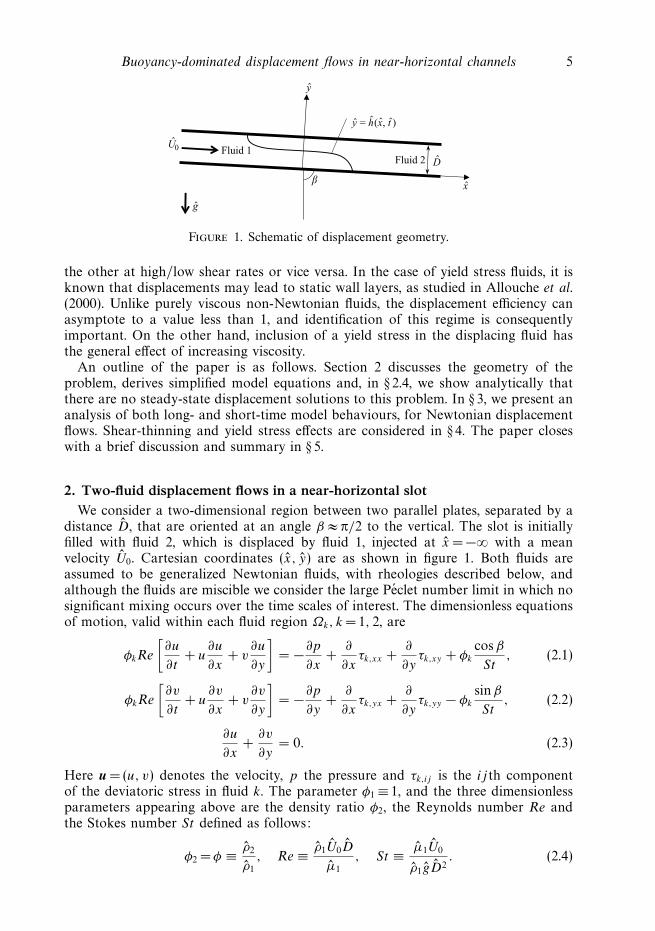
Figure 1. Schematic of displacement geometry.

the other at high/low shear rates or vice versa. In the case of yield stress fluids, it isknown that displacements may lead to static wall layers, as studied in Allouche et al.(2000). Unlike purely viscous non-Newtonian fluids, the displacement efficiency canasymptote to a value less than 1, and identification of this regime is consequentlyimportant. On the other hand, inclusion of a yield stress in the displacing fluid hasthe general effect of increasing viscosity.

An outline of the paper is as follows. Section 2 discusses the geometry of theproblem, derives simplified model equations and, in § 2.4, we show analytically thatthere are no steady-state displacement solutions to this problem. In § 3, we present ananalysis of both long- and short-time model behaviours, for Newtonian displacementflows. Shear-thinning and yield stress effects are considered in § 4. The paper closeswith a brief discussion and summary in § 5.

2. Two-fluid displacement flows in a near-horizontal slotWe consider a two-dimensional region between two parallel plates, separated by a

distance D, that are oriented at an angle β ≈ π/2 to the vertical. The slot is initiallyfilled with fluid 2, which is displaced by fluid 1, injected at x = −∞ with a meanvelocity U0. Cartesian coordinates (x, y) are as shown in figure 1. Both fluids areassumed to be generalized Newtonian fluids, with rheologies described below, andalthough the fluids are miscible we consider the large Peclet number limit in which nosignificant mixing occurs over the time scales of interest. The dimensionless equationsof motion, valid within each fluid region Ωk, k = 1, 2, are

φkRe

[∂u

∂t+ u

∂u

∂x+ v

∂u

∂y

]= −∂p

∂x+

∂

∂xτk,xx +

∂

∂yτk,xy + φk

cos β

St, (2.1)

φkRe

[∂v

∂t+ u

∂v

∂x+ v

∂v

∂y

]= −∂p

∂y+

∂

∂xτk,yx +

∂

∂yτk,yy − φk

sinβ

St, (2.2)

∂u

∂x+

∂v

∂y= 0. (2.3)

Here u = (u, v) denotes the velocity, p the pressure and τk,ij is the ij th componentof the deviatoric stress in fluid k. The parameter φ1 ≡ 1, and the three dimensionlessparameters appearing above are the density ratio φ2, the Reynolds number Re andthe Stokes number St defined as follows:

φ2 = φ ≡ ρ2

ρ1

, Re ≡ ρ1U0D

μ1

, St ≡ μ1U0

ρ1gD2. (2.4)


Here ρk is the density of fluid k, μ1 is a viscosity scale for fluid 1 and g

is the gravitational acceleration. Further dimensionless parameters will appear inconstitutive laws, defining the deviatoric stresses. In order to derive (2.1)–(2.3) wehave scaled distances using D, velocities with U0, time with D/U0, pressure andstresses with μ1U0/D.

On the walls of the slot the no-slip condition is satisfied. Due to the scaling adopted,we have ∫ 1

0

u dy = 1, (2.5)

in each cross-section. The slot is assumed infinite in x, with the interface betweenfluids initially localized close to x = 0. We shall consider flows that are buoyancydominated, in which the heavier fluid lies at the bottom of the slot, separated fromthe lighter upper fluid by an interface that we denote by y = h(x, t) and assume to besingle valued. Across the interface, velocity and stress are continuous. The interfaceis simply advected with the flow, satisfying a kinematic condition.

2.1. Constitutive laws

The fluids are assumed to be generalized Newtonian fluids. In particular we areinterested to understand shear thinning and yield stress effects. A suitable modelthat incorporates these effects is the Herschel–Bulkley model, which incorporates alsothe simpler Bingham, power law and Newtonian models. Constitutive laws for theHerschel–Bulkley fluids are

γ (u) = 0 ⇐⇒ τk(u) � Bk, x ∈ Ωk, (2.6)

τk,ij (u) =

[κkγ

nk−1(u) +Bk

γ (u)

]γij (u) ⇐⇒ τk(u) > Bk, x ∈ Ωk, (2.7)

where the strain rate tensor has components

γij (u) =∂ui

∂xj

+∂uj

∂xi

, (2.8)

and the second invariants γ (u) and τk(u) are defined by

γ (u) =

[1

2

2∑i,j=1

[γij (u)]2

]1/2

, τk(u) =

[1

2

2∑i,j=1

[τk,ij (u)]2

]1/2

. (2.9)

Herschel–Bulkley fluids are described by three-dimensional parameters: a fluidconsistency κ , a yield stress τY and a power law index n. The parameter κ1 = 1and κ2 is the viscosity ratio m:

m ≡ μ2

μ1

=κ2[U0/D]n2−1

κ1[U0/D]n1−1, (2.10)

where μ2 is a viscosity scale for fluid 2. Note that in the case of two Newtonian fluids,μk = κk . The Bingham numbers Bk are defined as

Bk ≡ τk,Y

κ1[U0/D]n1

. (2.11)

2.2. Buoyancy dominated flows: |φ − 1|/St � 1

The objective of our study is to understand a particular limit of (2.1)–(2.3), in whichinertia is not considered to be dominant and the interface orients approximately


horizontally along the axis of the slot: moderate Re, β ≈ π/2 and φ ∼ O(1). The ratioof buoyancy to viscous forces is given by the parameter |φ − 1|/St . We suppose that|φ − 1|/St � 1 so that the interface elongates over some (dimensionless) length scaleδ−1 � 1. To define this length scale we assume that the dynamics of spreading ofthe interface, relative to the mean flow, will be driven by buoyant stresses whichhave size: |ρ1 − ρ2|g sinβD in the y direction. These stresses, which act across theinterface where there is a density difference, translate into axial stresses accordingto the slope of the interface. If the slope of the interface has size D/L, the stressthat acts to spread the flow axially has size |φ − 1|ρ1g sinβD2/L. This tendency to

spread is resisted by viscous stresses within the fluids, of size μ1U0/D, which dissipatethe energy injected by buoyancy. By matching these two terms, we can obtain thecharacteristic spreading length in this regime:

|φ − 1|ρ1g sinβD2/L = μ1U0/D ⇒ L =|φ − 1|ρ1g sinβD3

μ1U0

. (2.12)

Thus, the ratio between the axial length scale and channel width is

δ−1 =L

D=

|φ − 1|ρ1g sinβD2

μ1U0

=|φ − 1| sinβ

St. (2.13)

Following standard methods (see, e.g. Leal 2007) we rescale as follows:

δx = ξ, δt = T , δp = P, v = δV,

and arrive at the following reduced system of equations, in each fluid regionΩk, k = 1, 2:

δφkRe

[∂u

∂T+ u

∂u

∂ξ+ V

∂u

∂y

]= −∂P

∂ξ+

∂

∂yτk,ξy + φk

cosβ

St+ O(δ2),

δ3φkRe

[∂V

∂T+ u

∂V

∂ξ+ V

∂V

∂y

]= −∂P

∂y− δφk

sinβ

St+ O(δ2),

∂u

∂ξ+

∂V

∂y= 0.

To aid interpretation of our model results, note that the time and length variables(T , ξ ) are related to the dimensional time and length by

|ρ1 − ρ2|g sinβD3

μ1U0

ξ = x,|ρ1 − ρ2|g sinβD3

μ1U20

T = t . (2.14)

Note that we have used D/U0 to scale t , which is the usual convective time scale basedon the mean velocity and D. Therefore, the scale related to the slow time variable T

corresponds to the time taken to travel the characteristic spreading length L at meanvelocity U0.

We now consider the limit δ → 0 with Re fixed:

0 = −∂P

∂ξ+

∂

∂yτk,ξy + χ

φk

|1 − φ| , (2.15)

0 = −∂P

∂y− φk

|1 − φ| , (2.16)


Light Heavy

Heavy LightU0

U0

(a)

(b)

Figure 2. Schematic of displacement types considered: (a) heavy fluid displaces light fluid(HL displacement); (b) light fluid displaces heavy fluid (LH displacement).

where χ = cot β/δ. The parameter χ measures the relative importance of the slopeof the channel to the slope of the interface, in driving buoyancy related motions. Wewish to consider channels that are close to horizontal, where the slopes of both thechannel and the interface may be of comparable importance. Thus, we assume χ is anorder 1 parameter, i.e. we consider inclinations β = π/2+O(δ). For χ > 0 the slope ofthe channel is ‘downhill’, in the direction of the flow, and for χ < 0 the flow is uphill.Note that for larger χ the model does not necessarily break down, but effectively wehave chosen the wrong scaling as the effect of the channel slope is dominant.

Before proceeding, we observe that there are two qualitatively different types ofdisplacement flows:

(a) HL (heavy–light) displacement: fluid 1 is heavier than fluid 2, and the lowerlayer of fluid is consequently fluid 1. Parameters are (nH , κH , BH , nL, κL, BL) =(n1, 1, B1, n2, m, B2).

(b) LH (light–heavy) displacement: fluid 1 is lighter than fluid 2, and the lowerlayer of fluid is consequently fluid 2. Parameters are (nH , κH , BH , nL, κL, BL) =(n2, m, B2, n1, 1, B1).These are illustrated schematically in figure 2. We do not consider mechanicallyunstable configurations, i.e. heavy fluid over light fluid.

We integrate (2.16) across both fluid layers to give the pressure:

P (ξ, y, T ) =

⎧⎪⎪⎨⎪⎪⎩

P0(ξ, T ) + χφH

|1 − φ|ξ − φH

|1 − φ|y y ∈ [0, h],

P0(ξ, T ) + χφH

|1 − φ|ξ − φH − φL

|1 − φ| h − φL

|1 − φ|y y ∈ [h, 1],

(2.17)where P0(ξ, T ) is defined by

P0(ξ, T ) = P (ξ, 0, T ) − χφH

|1 − φ|ξ,

with φH = ρH /ρ1 for the heavier fluid, φL = ρL/ρ1 for the lighter fluid. On substitutinginto (2.15), we arrive at

0 = −∂P0

∂ξ+

∂

∂yτH,ξy, y ∈ (0, h), (2.18)

0 = −∂P0

∂ξ+

∂

∂yτL,ξy − χ +

∂h

∂ξ, y ∈ (h, 1). (2.19)

In the lubrication approximation, the leading order strain rate component isγξy = ∂u/∂y, and the leading order shear stress τk,ξy is defined in terms of γξy via the


following leading order constitutive laws:

∂u

∂y= 0 ⇐⇒ |τk,ξy | � Bk, x ∈ Ωk, (2.20)

τk,ξy =

⎡⎢⎢⎣κk

∣∣∣∣∂u

∂y

∣∣∣∣nk−1

+Bk∣∣∣∣∂u

∂y

∣∣∣∣

⎤⎥⎥⎦ ∂u

∂y⇐⇒ |τk,ξy | >Bk, x ∈ Ωk. (2.21)

Thus, for given h and ∂h/∂ξ , (2.18) and (2.19) define an elliptic problem for u(y).Boundary conditions for u(y) are u =0 at y = 0, 1. At the interface, y = h, u iscontinuous and τH,ξy = τL,ξy , representing stress continuity. These four conditions aresufficient to determine u for given ∂P0/∂ξ . The pressure gradient is determined by theadditional constraint that (2.5) is satisfied.

For now we assume that the solution of this problem may be computed and wenote that the dependence of u on (ξ, T ) enters only via h(ξ, T ), which satisfies

∂h

∂T+ u

∂h

∂ξ= V. (2.22)

Combining the kinematic equation with the divergence free constraint leads, in theusual manner, to the equation

∂h

∂T+

∂

∂ξq(h, hξ ) = 0, (2.23)

where q(h, hξ ) is defined as

q(h, hξ ) =

∫ h

0

u(y, h, hξ ) dy. (2.24)

The remainder of our study concerns behaviour of solutions to the system (2.23) and(2.24).

As boundary conditions, for an HL displacement we have that

h(ξ, T ) → 1, as ξ → −∞; h(ξ, T ) → 0, as ξ → ∞, (2.25)

as the channel is assumed full of pure fluid 1 and fluid 2 at the two ends ofthe channel. As initial conditions we note that an initial profile in the unscaledvariables h(x, t = 0) = h0(x) is transformed to h(ξ, T = 0) = h0(ξ/δ). Since h0 shouldbe compatible with the far-field conditions we have that as δ → 0,

h(ξ, 0) → 1 − H (ξ ), (2.26)

where H (ξ ) is the usual Heaviside function. In other words, in terms of ξ , the initialchange in h is localized to ξ = 0. For an LH displacement this is reversed, i.e.

h(ξ, T ) → 0, as ξ → −∞; h(ξ, T ) → 1, as ξ → ∞, (2.27)

h(ξ, 0) = H (ξ ), (2.28)

since the far-field pure fluids are reversed.

2.3. The flux function q(h, hξ )

In the general case, finding the flux function q(h, hξ ) requires computation, and this isaddressed in Appendix A. For the particular case of a Newtonian fluid the analytical


(a)

(c)

(b)

(d)

0 0.2 0.4 0.6 0.8 1.0

0.2

0.4

0.6

0.8

1.0

q

0.2 0.4 0.6 0.8 1.00

0.2

0.4

0.6

0.8

1.0

0 0.2 0.4 0.6 0.8 1.0

0.2

0.4

0.6

0.8

1.0

h

q

0 0.2 0.4 0.6 0.8 1.0

0.2

0.4

0.6

0.8

1.0

h

Figure 3. Examples of q for two Newtonian fluids: (a) b = 0 and different m; HL displacementwith m= 0.1 (�), m= 1 (�), m= 10 (�); LH displacement with m= 10 (�), m= 1 (�), m= 0.1(�); (b) m= 1 and different b; HL or LH displacements with b = −10 (�), b = 0 (�), b = 10(�). Examples of q for two non-Newtonian fluids in HL displacement: (c) b = 1, m= 1, B2 = 1,nk = 1, B1 = 0 (�), B1 = 5 (�), B1 = 10 (�), B1 = 20 (�); (d ) b = 1, Bk = 1, nk = 1, m= 0.1 (�),m= 1 (�), m= 10 (�).

solution may be found trivially. Denoting b = χ −hξ , for an HL displacement we find

q(h; b, m) = qA(h; m) + bqB(h; m). (2.29)

where qA(h; m) and qB(h; m) represent the advective and buoyancy-driven componentsof the flux q(h; b, m):

qA(h; m) =3mh2(mh2 + (h + 3)(1 − h))

3[(1 − h)4 + 2mh(1 − h)(h2 − h + 2) + m2h4], (2.30)

qB(h; m) =[h3(1 − h)3(mh + (1 − h))]

3[(1 − h)4 + 2mh(1 − h)(h2 − h + 2) + m2h4]. (2.31)

For an LH displacement, the flux function is given by

q(h; b, m) = qA(h; 1/m) + bqB(h; 1/m). (2.32)

Examples of computed q are given in figure 3. For all examples, these functionshave been computed using the procedure described in Appendix A, with the resultscompared against (2.29) in the case of Newtonian fluids, to verify the numericalmethod.

We observe that the curves for m =0.1 and m = 10 in figure 3(a), (with b = 0), showa reflective symmetry, as do those for b = ± 10 in figure 3(b), (with m = 1). Note alsothat in figures 3(a) and 3(b), the flux functions are relevant to both HL and LH


displacements, but with m replaced by 1/m in the case of LH displacements. Thisapparent symmetry between HL and LH displacements is not obvious. Note thatalthough the fluxes are mathematically identical for the same b, in fact b = χ −hξ willnot be the same since hξ will have different sign between the two displacement types.In addition, m is the ratio of displaced to displacing fluid viscosity, which changeswith the displacement type. In other words, replacing m with 1/m and switching fromHL to LH does give the same q , but does not give the same ‘shape’ of interface(meaning that we replace h with 1 − h, since the LH displacement front slumps alongthe top of the channel). Instead the HL and LH interfaces are the same shape for thesame m in the case of a horizontal channel χ = 0, (see figures 4c and 4d ), and willbe the same shape for small inclinations if we retain the same m and replace χ with−χ . This does not therefore contradict observations from lubrication-type models ofisodensity displacements with central finger-like interfaces, where the cases m and1/m also produce markedly different results.

Figures 3(c) and 3(d ) illustrate non-Newtonian effects on q in HL displacements.In figure 3(c) we observe that as the heavy fluid yield stress B1 is increased q =0 insome interval of small h. For these thin layers the yield stress fluid remains static.In figure 3(d ) we see that the effects of viscosity ratio m is broadly similar for non-Newtonian and Newtonian fluids. For the examples shown, q increases monotonicallywith little apparent effect of varying the parameters. This is however not always thecase, as we have presented only a limited subset of the six parameters, mostly ofO(1). With more slightly extreme parameter combinations it is not difficult to find q

that are non-monotone, for example. We shall see later that most of the qualitativeinformation concerning the long-term behaviour of the solution is contained in ∂q/∂h,for which the differences are significant.

2.4. The existence of steady travelling wave displacements.

One of the most important practical questions in considering this displacement flowis whether or not (2.23) and (2.24) admit steady travelling wave solutions. Thisdetermines whether or not the displacement can be effective. In this section wedemonstrate that, regardless of fluid type and of rheological differences betweenfluids, it is impossible for there to be a steady travelling wave solution. Havingdiscounted this possibility, in later sections we turn to a qualitative description of thesolutions for different fluid types.

First, let us note that the slope of the interface hξ acts always to spread the interface.To see this note that following the construction of the previous section, we may writeq(h, hξ ) = q(h, b) where b = χ − hξ . Formally we may write (2.23) as

∂h

∂T+

∂q

∂h

∂h

∂ξ= −∂q

∂b

∂b

∂ξ=

∂q

∂b

∂2h

∂ξ 2, (2.33)

from which we see that the interface spreads diffusively provided that q(h, b) increaseswith b. We prove the following result in Appendix B.

Lemma 1. q(h, b) is non-decreasing for all b.

Now we examine the condition for there to be a steady travelling wave solution.Since fluid 1 is injected at mean speed 1, the only steady speed that needs be consideredis unity. Shifting to a moving frame of reference, say z = ξ − T , we see that if thesolution is steady in this frame h = h(z), we must have that

d

dz

[h − q

(h, χ − dh

dz

)]= 0,


and since q =0 at h = 0, this implies that

h = q

(h, χ − dh

dz

), (2.34)

must be satisfied for all h ∈ [0, 1] if there is to be a steady travelling wave solution.For an HL displacement we impose the further conditions that h(z) decreasesmonotonically from 1 to 0 with z. For an LH displacement these conditions arereversed: h(z) increases monotonically from 0 to 1 with z. Using Lemma 1, withb =χ − dh/dz we see that the following is true.

Lemma 2. For an HL displacement, a necessary condition for there to be steadytravelling wave solution is that q(h, χ) � h for all h ∈ [0, 1]. For an LH displacement,a necessary condition for there to be steady travelling wave solution is that q(h, χ) � h

for all h ∈ [0, 1].

This follows directly since for an HL displacement we require that dh/dz � 0 sothat q(h, b) � q(h, χ). If this condition is not satisfied we would therefore be unable tofind a solution to (2.34), similarly for the LH displacement. Following the proceduresin Carrasco-Teja et al. (2008) we can in fact show that the conditions of Lemma 2are in fact sufficient as well as necessary.

Finally, we shall show that the conditions of Lemma 2 are in fact never satisfied.We focus only on the HL displacement, the LH displacement being treated similarly.We consider solutions u(y) to the system

∂

∂yτH,ξy = −f, y ∈ (0, h),

∂

∂yτL,ξy = χ − f, y ∈ (h, 1),

for any of the constitutive laws, with no slip at the walls and continuity of stress andvelocity at y = h, plus the flow rate constraint (2.5), which determines f . We fix χ

and consider h = 1 − ε, noting first that both the velocity solution and f (h) will varysmoothly with h. For any h ∈ [0, 1] we note that the shear stress throughout the lightfluid layer is given by

τL,ξy(y; h) = τL,ξy(1; h) + (1 − y)(f (h) − χ),

and as h → 1, we have

τL,ξy(y; h) ∼ τL,ξy(1; 1) − ε∂τL,ξy

∂h(1; 1) + ε(f (1) − χ) + O(ε2).

Thus, the velocity gradient within the light fluid layer is given by

∂u

∂y=

∂u

∂y(τL,ξy(1; 1)) + O(ε),

where the algebraic relation for the velocity gradient comes directly from theconstitutive laws. Hence we may straightforwardly compute the flux in the lighterfluid layer:

qL(ε) =

∫ 1

h

u(y)dy ∼ −ε2

2

∂u

∂y(τL,ξy(1; 1)) + O(ε3).

Now when h = 1 the channel is full with the heavy fluid, and the pressure gradientcorresponds to the Poiseuille flow solution, say f (1) = fH (1) > 0, which can be easily


calculated. The stress at the upper wall is thus −0.5fH (1) and since the shear stressis continuous we have

τL,ξy(1; 1) = − 0.5fH (1) < 0 ⇒ qL(ε) ∼ −ε2

2

∂u

∂y(−0.5fH (1)) > 0.

Since via the flow rate constraint we have that the total flux is equal to unity, wehave that

q(h, χ) ∼ 1 +(1 − h)2

2

∂u

∂y(−0.5fH (1)) > h, as h → 1. (2.35)

Consequently for an HL displacement the necessary conditions of Lemma 2 are alwaysviolated sufficiently close to h =1, regardless of fluid type and rheological differences.Similarly, we can show that for an LH displacement the necessary conditions ofLemma 2 are always violated sufficiently close to h = 0, regardless of fluid type andrheological differences. This leads to the following result.

Lemma 3. There are no steady travelling wave solutions to (2.23).

Remarks:(i) This is the key theoretical result of the paper. It is perhaps surprising that for

no combination of rheology or density differences are we able to achieve a ‘perfect’displacement, (under the assumptions of the lubrication displacement model). Thischanges the focus of the study. First, in order to achieve a good displacement,we are driven to study those parameter combinations that give the best efficiency,close to 100 %. Second, if we wish to improve the efficiency we need considerphenomena that might do this, other than those accounted for in this simplisticmodel, e.g. hydrodynamic instability and mixing, or the short-time dynamics in theinterfacial region before the interface slumps.

(ii) For a Newtonian fluid displacement, we might find this result rather moredirectly as the solution may be computed. For example, in Seon et al. (2007) thesimpler problem of two Newtonian fluids of identical viscosity in an inclined pipeis considered, in the absence of a mean imposed flow. No travelling wave solutionsare found. Here, however, the mean flow results in a different structure to the fluxfunctions q , i.e. for Newtonian fluids the advective and buoyant components qA

and qB are present whereas only qB is present in Seon et al. (2007), (also with analgebraically different form). For non-Newtonian fluids the division of the flux intoqA and qB is not possible, due to nonlinearity. Thus, we have to work with qualitativeproperties of the fluxes for such fluids. While we might anticipate from results suchas Seon et al. (2007) that no travelling waves solutions to (2.23) can be found, froma physical perspective addition of a constant volume flux (i.e. a displacement) makesthis a natural and legitimate question.

(iii) Although we have focused on Herschel–Bulkley fluids for definiteness, thesame results could be demonstrated for any of the popular generalized Newtonianmodels, e.g. Carreau fluids, Cross model, Casson model, etc.

3. Newtonian fluidsWe commence with an analysis of Newtonian fluid displacements. Although the

industrial applications discussed in § 1 typically involve non-Newtonian fluids, manyof the qualitative behaviours are exhibited in a Newtonian fluid displacement. Analysisof the Newtonian fluid case not only provides simplification in terms of the number


(a)

(c) (d)

(b)

0 0.5

ξ

1.0 1.50

0.2

–0.5

0.4

0.6

0.8

1.0

h(ξ, T

)

ξ/T

ξ/T ξ/T

0 0.5–0.5–1.0 1.0 1.5 2.00

0.2

0.4

0.6

0.8

1.0

h

0.1–0.1 –0.10.3 0.5 0.7 0.9 0.11 1.3 1.50

0.2

0.4

0.6

0.8

1.0

h

0 0.5 1.1 1.50

0.5

1.0

0.1 0.3 0.5 0.7 0.9 1.1 1.3 1.50

0.2

0.4

0.6

0.8

1.0

h

0 0.5 1.0 1.50

0.5

1.0

Figure 4. Examples of HL displacements: (a) h(ξ, T ) for T = 0, 0.1, . . . , 0.9, 1, parametersχ = 0, m= 1; (b) h(ξ/T ) for T = 1, . . . , 9, 10, parameters χ = 0, m= 1. Examples of HLdisplacements: (c) h(ξ/T ) for χ = 0: m= 0.1 (�), m= 1 (�), m= 10 (�); (d ) h(ξ/T ) for m= 1:χ = −10 (�), χ = 0 (�), χ =10 (�). The inset figures in (c) and (d ) show the results of LHdisplacements for the same parameters.

of dimensionless parameters, i.e. (m, χ), but also since q is given by the analyticalexpression (2.29) numerical solution is considerably faster. For non-Newtonian fluids,each evaluation of q requires numerical solution of the nested iteration described in§ A.

The convection–diffusion equation (2.23) was discretized in the conservativeform, second order in space and first order in time; and afterward, integratedstraightforwardly by using a Lax–Wendroff scheme in which an artificial dissipationwas added to the equation to recover the destabilizing effects of the known anti-diffusion due to the first-order time discretization. The only unsatisfactory aspect ofthe method applied was a small amount of smoothing close to the sharp front tip ofthe interface. This feature was found to be consistent with time since the flux functionand added dissipation vanish in both walls.

3.1. Examples of typical qualitative behaviour

Example computed HL displacements are shown in figure 4. The results at longtimes are not found to be particularly sensitive to the initial condition, which wehave taken as a linear function of ξ : typically h(ξ, T = 0) = ∓ξ ± 0.5 for HL and LHdisplacements, respectively. When we have wished to study the early-time evolutionof the interface, we steepen the initial profile, e.g. in figure 4(a) the initial conditionis h(ξ, T = 0) = −ξ + 0.05. Figures 4(a) and 4(b) plot the solution for m =1, χ =0,(i.e. equal viscosities in a perfectly horizontal channel). In the early times, T ∈ [0, 1]


we observe that the interface develops quickly into a slumping profile; see figure 4(a).Over longer times, the solution consists of two segments: an advancing front ofapparently constant shape moving at constant speed and a region at the top whichis stretched, the top of the interface simply not moving. The longer time profiles ofh may be conveniently plotted against ξ/T , in which variable the interface profilescollapse to a single similarity profile as T → ∞ (figure 4b). To clarify interpretation offigures such as figure 4(b), the x-axis of the final similarity profile gives the speed ofthe interface at different heights: vertical lines correspond to segments of the interfacethat advance at steady speed.

Note that the first interface profile in figure 4(b), for T = 1, effectively shows h(ξ, T )at T = 1, and in this we may observe that the top of the interface is pinned tothe upper wall at the initial position ξ = −0.5. The convergence at the upper wallas T → ∞ simply follows ξ/T = −0.5/T , and the interface itself does not move, asevidenced in figure 4(a) over shorter times. Thus, the apparent discrepancy betweenthe last interface profile of figure 4(a) and the first interface profile of figure 4(b) issimply due to the different initial conditions.

This qualitative behaviour is similar for other parameters and indeed convergenceto the ‘final’ similarity profile is relatively quick, occurring over an O(1) time scale(in T ). For our other results we present only the interface at T = 10, which is alwaysvery close to the final similarity profile. Figure 4(c) shows the final shape for threedifferent values of viscosity ratio m and figure 4(d ) shows the final shape for threedifferent values of the inclination parameter χ . For larger m the height of the steadilymoving front, say hf , is smaller. This is intuitive, since increasing m correspondsto an increasingly less viscous fluid displacing a more viscous fluid. The interfaceabove the steadily moving front also transitions from convex to concave curvatureas m is increased, further emphasizing the extending finger. Similarly, for χ > 0 theheavy fluid flows downhill through the lighter fluid and hf is accordingly smallerin this configuration. The inset figures in figures 4(c) and 4(d ) show the analogousLH displacements for the same parameters. The effects of m are identical with thosefor the HL displacement, (since m is the ratio of in-situ fluid viscosity to displacingfluid viscosity). The effect of varying χ is however reversed: χ > 0 retards unsteadyspreading for an LH displacement and χ < 0 promotes unsteady spreading.

3.2. Long-time behaviour

We have seen in figure 4 that the interface tends to evolve on an O(1) time scaleinto a shape that consists of two parts: (i) a front region that remains approximatelyconstant but advances at steady speed; (ii) a stretched region, in which the interfaceis continually extended, as t → ∞. For the HL displacement the steadily movingfront occupies the lower part of the channel, and for the LH displacement the frontadvances along the upper wall. In place of computations, we would like to directlycompute this long-time behaviour. In what follows below we focus for simplicity onthe HL displacements.

We commence with the upper stretched region. If we denote the steady front heightand speed by hf and Vf , respectively, we observe that at long times the slope of theinterface is approximately

∂h

∂ξ∼ −1 − hf

Vf T→ 0, as T → ∞.


Therefore, as T → ∞, we have that b = χ − ∂h/∂ξ → χ , and the interface motion inthe stretched region is governed approximately by

∂h

∂T+

∂

∂ξq(h, χ) = 0, (3.1)

which is hyperbolic rather than parabolic. The interface in this region advances withspeed Vi(h) given by

Vi(h) =∂q

∂h(h, χ).

Thus, the total area of fluid flowing behind the interface in the interval [hf , 1] at longtimes is

T

∫ 1

hf

Vi(h) dh = T [1 − q(hf , χ)].

Furthermore, at the front height hf the interface speed should equal the front velocityVf , i.e.

∂q

∂h(hf , χ) = Vi(hf ) = Vf . (3.2)

The total area of fluid behind the interface is T and since the area of fluid flowingbehind the interface in the interval [0, hf ] is approximately T Vf hf , we have thefollowing relationship:

T q(hf , χ) = T − T [1 − q(hf , χ)] = T Vf hf = T hf

∂q

∂h(hf , χ),

from which

q(hf , χ) = hf

∂q

∂h(hf , χ). (3.3)

Equation (3.3) is an equation for the front height hf . This is instantly recognizable asthe same condition that must be satisfied in the case of a kinematic shock, in orderto conserve mass. Therefore, note that the long time behaviour is that determined bythe underlying hyperbolic conservation law.

An example of the use of the equal areas rule (3.3) to determine the front heightis shown in figure 5(a). In figure 5(b) we plot h against ξ/T for T = 1, . . . , 9, 10,showing that hf does indeed represent the moving front, which has the same speedas indicated in figure 5(a). Although for most of the parameters we have considered,there is a single propagating front, some parameters result in a double front. Looselyspeaking, for Newtonian fluids this appears to arise at more extreme parameter valueswhen physical effects are somehow opposing one another. An example is shown inFigures 5(c) and 5(d ). In this illustration, the competing effects are buoyancy, drivenby the downhill slope which acts to spread the interface, and the viscosity ratio whichacts to sharpen the front.

Figure 6(a) shows calculated front heights for HL and LH displacements fordifferent values of χ and m. To interpret this figure for the LH displacement Thefront height hf for LH displacement is defined as the distance from the top wallto the stretched part of the interface. We observe that higher viscosity ratios tendto have a lower front height, which simply means that in order to have a moreefficient displacement, the displacing fluid should be more viscous in comparison tothe displaced fluid. Increasing χ tends to reduce efficiency for the HL displacementbut increase efficiency for the LH displacement. Via repeated computation of q fordifferent (m, χ) we are able to delineate the regime in the (m, χ) plane in which


0.2 0.4 0.6 0.8 1.00

0.5

1.0

1.5

2.0

2.5(a) (b)

(c) (d)

∂q/∂

h

0.5

1.0

1.5

2.0

2.5

∂q/∂

h

0–0.5–1.0 0.5 1.0 1.5 2.00

0.2

0.4

0.6

0.8

1.0

h

0

0.2

0.4

0.6

0.8

1.0

h

0.2 0.4 0.6 0.8 1.00

h ξ/T0–0.5–1.0 0.5 1.0 1.5 2.0

Figure 5. Use of the equal areas rule (3.3) in determining the front height: (a) a single frontheight, χ =10,m= 8; (b) h plotted against ξ/T for T = 1, . . . , 9, 10, parameters χ =10,m= 8,broken horizontal line indicates the front height determined from (3.3); (c) two front heights,χ = 10,m= 0.08; (d ) h plotted against ξ/T for T = 1, . . . , 9, 10, parameters χ = 10,m= 0.08,broken horizontal lines indicate the front heights.

10–1 100 1010.5

0.6

0.7

0.8

0.9

1.0(a) (b)

m

hf

010–1 100 101

m

10

20

30

40

χ

50

Figure 6. (a) Front heights for a Newtonian fluid HL displacement with χ = −10 (�),χ = −5 (�), χ =0 (�), χ =5 (�), χ =10 (�). This figure also gives the front heights fora Newtonian fluid LH displacement with χ = 10 (�), χ = 5 (�), χ = 0 (�), χ = −5 (�),χ = −10 (�). For the LH displacement the front height is measured down from the top wall;(b) Parameter regime in the (m,χ) plane in which multiple fronts (shaded area). Elsewherethere is only a single front.

multiple fronts are found (figure 6b). Within the shaded region of figure 6(b), notethat some parameter values give front speeds that are negative, i.e. there is a backflowdriven by buoyancy.

Although the expression (3.3) for the front height is exactly the equation that wouldbe solved for computing a kinematic shock for the hyperbolic conservation law, it is


0 0.1–0.1–0.2–0.3–0.40

0.2

0.4

0.6

0.8

1.0

0

0.2

0.4

0.6

0.8

1.0

z0 0.1–0.1–0.2–0.3–0.4–0.5

z

h

(a) (b)

Figure 7. Examples of front shapes in the moving frame of reference for an HL displacement,computed from (3.4): (a) χ = 0, m= 0.1 (�),m= 1 (�),m= 10 (�); (b) χ = −10 (�), χ = −5 (�),χ = 0 (�), χ = 5 (�), χ = 10 (�). Compare with transient computations in Figures 4(c) and4(d ).

important to emphasize that the front is not a shock since diffusive effects are alwayspresent for h ∈ (0, 1). Having determined hf from (3.3) and then Vf from (3.2), wemay shift to a moving frame of reference z = ξ − Vf T and seek a steadily travellingsolution to (2.23), which satisfies

d

dz

[hVf − q

(h, χ − dh

dz

)]= 0, ⇒ hVf − q

(h, χ − dh

dz

)= 0. (3.4)

Equation (3.4) must be solved numerically for h ∈ (0, hf ). Example shapes are shownin figure 7. Figure 7(a) shows HL displacement front shapes for two Newtonian fluidsfor different values of viscosity ratio at χ = 0. Figure 7(b) shows HL displacementfront shapes for two Newtonian fluids for different values of χ at m = 1. These are thesame parameters as for the transient displacements in Figures 4(c) and 4(d ). Observefrom (3.4) as h → h−

f that, since hf is determined from (3.3) and Vf from (3.2), wemust have

q

(h, χ − dh

dz

)→ q(hf , χ) as h → h−

f ,

which implies that dh/dz → 0 as h → h−f , as can be seen in figure 7. Evidently, as

T → ∞ the stretched region of the interface also aligns horizontally, so that thelong-time solution is smooth at hf .

3.3. Flow reversal and short-time behaviour

The model results presented so far have been derived under lubrication scalingassumptions, with the length scale determined by dominant buoyancy effects,compatible with the assumed stratification. Our study of the long-time behaviourhas revealed only forward propagating fronts, which of course are more commonsince a positive flow rate is imposed. If the channel is horizontal then, as the frontadvances and the slope of the interface decreases, the driving force to oppose themean flow also diminishes. Thus, we cannot expect flow reversal in a horizontalchannel at long times.

On the other hand, with an inclined channel there is a constant buoyancy force thatmay either reinforce or oppose the mean flow. For example, with an HL displacementat fixed positive inclination, χ > 0, buoyancy acts to push the lighter fluid against themean flow direction. For sufficiently large χ and small viscosity ratio, we observe that


0–5–10–15 5 10 15 20 25 300

0.2

0.4

0.6

0.8

1.0

ξ

h(ξ, T

)

Figure 8. Profiles of h(ξ, T ) for T =0, 1, . . . , 9, 10, with parameters χ =50, m= 0.1,illustrating flow reversal.

the lighter fluid may be driven backwards against the flow, resulting in a sustainedflow reversal. An example of this is shown in figure 8.

Flow reversal may also be observed in other situations. The most obvious of these isthe case T � 1, since for short times large interface slopes may mean that gravitationalspreading may dominate the imposed flow. Since our model is anyway an asymptoticreduction of the full equations in which T effectively represents a long-time relativeto the advective time scale over the channel width, the limit T → 0 is one in whichthe underlying assumptions of the model break down. Nevertheless, the problem forT � 1 is mathematically well defined and of physical interest.

To study this limit, we shift to the steadily moving frame of reference z = ξ − T ,recall that b = χ − hξ , and consider (2.23) for an HL displacement, which becomes

∂h

∂T+

∂

∂z

[qA(h; m) +

(χ − ∂h

∂z

)qB(h; m) − h

]= 0, (3.5)

where qA(h; m) and qB(h; m) represent the advective and buoyancy-driven componentsof the flux q(h; b, m), which is defined by (2.29) for two Newtonian fluids, i.e.introducing η = z/

√T this becomes

1

2ηdh

dη−

√T

d

dη(qA − h + χqB) + qB

d2h

dη2+

∂qB

∂h

(dh

dη

)2

= 0. (3.6)

Therefore, provided that T ∼ 0 we may seek a similarity solution satisfying

1

2ηdh

dη+ qB

d2h

dη2+

∂qB

∂h

(dh

dη

)2

= 0, (3.7)

or in conservative form

1

2ηdh

dη=

d

dη

(−qB

dh

dη

). (3.8)

Since qB(h; m) vanishes at both h = 0 and h = 1, it is clear that there is somesingular behaviour in h(η) at these points. Thus, it is more comfortable to work withthe function η(h). The boundary conditions are η(0) = η0 and η(1) = η1, where η0 andη1 are unknown at this stage. Physically, we expect that η0 > 0 and η1 < 0 as thespreading of the interface is caused by gravitational slumping. A Taylor expansionreveals that η(h) ∼ η0 + O(h3) as h → 0, with similar asymptotic behaviour as h → 1,


0.1 0 0.2 0.4–0.2–0.4–0.1–0.3–0.5 0.3 0.50

0.2

0.4

0.6

0.8

1.0

0

0.2

0.4

0.6

0.8

1.0

η η

h(η)

m = 100

m = 0.01

T = 0.001

T = 0.1

(a) (b)

Figure 9. (a) the similarity solution h(η) for m= 0.01, 0.1, 1, 10, 100; (b) comparison of thesimilarity solution with the numerical solution of (3.5) for m= 1, at T = 0.001, 0.01, 0.1.

i.e. η′(h) → 0 quadratically at both ends of the interval. We integrate (3.8) as follows:

1

2ηdh = d

(−qB

dh

dη

), (3.9)

∫ h

0

1

2ηdh =

∫ h

0

d

(−qB

dh

dη

)= −qB(h)

dh

dη+ qB(0)

dh

dη= − qB(h)

dh

dη, (3.10)

(note qB(h) → 0 as h → 0 with order h3). Now taking h → 1 and using the asymptoticbehaviour qB(h) ∼ (1 − h)3, we have

1

2

∫ 1

0

η dh = 0. (3.11)

Let us now define g(h) such that η = g′. Therefore,

g(h) − g(0) =

∫ h

0

η · dh, (3.12)

and from (3.11), we see that g(1) = g(0). For convenience, we set g(0) = 0 so that(3.10) may be written as

g′′ · g = −2qB. (3.13)

We use the initial condition g(0) = 0 and g′(0) = η0. We then integrate forwards, withrespect to h and iterate on η0 via a shooting method to satisfy g(1) = 0.

This numerical procedure appears to work well. Figure 9(a) plots the similaritysolutions η(h) for various m. Note that the solution is not symmetric with respect tom. For the heavy–light displacement the heavy fluid viscosity is 1 and the light fluidviscosity is m. Buoyancy effects have no bias between the fluids, but the more viscousfluids evidently resist motion. Thus, we see that for large m the axial extension η0 −η1

is smaller than for small m. This effect might have been removed had we scaledviscosity with an appropriate mean value. A symmetrical shape is of course found atm =1.

These solutions have been compared with the solution of PDE equation (3.5) asT ∼ 0 and agree well for short times. An example is shown in figure 9(b) for the casem =1. Mathematically, these solutions serve primarily to demonstrate that for shorttimes, (e.g. after opening a gate valve in an experiment), buoyancy dominates andan exchange flow should occur, relative to the mean displacement. For smaller meanvelocities the parameter δ → 0 and the dimensional time period over which buoyancy


dominates extends to infinity, ensuring compatibility with exchange flow studies, forwhich there is zero net flow rate and hence a flow reversal in each layer.

To explore this analogy further, let us fix β = π/2, in which case we may note thatthe similarity variable η is defined in terms of dimensional variables by

η =z

T 1/2=

x − U0 t

t1/2

√μ1

|ρ1 − ρ2|gD3.

We may compare this with the analysis in Seon et al. (2007) for exchange flows inhorizontal pipes, wherein diffusive similarity profiles are found for Newtonian fluidsof the same viscosity. We may note that the scaling |ρ1 − ρ2|gD3/μ1 is the same asthe (Vνd)1/2 that scales the similarity variable x/t1/2 in Seon et al. (2007) (see (27) and§ VII.B in this paper). However, although this is the same viscous-buoyancy balancedriving the diffusive spreading in both cases, here we have the additional criterionthat T 1/2 � 1, and we have seen numerically that the diffusive regime does not lastfor longer times. This criterion can be written dimensionally as

t U0

D� 1

U0

|ρ1 − ρ2|gD2

μ1

=L

D.

The most simplistic interpretation therefore is that t U0 � L , i.e. the distance advectedduring the time considered must be much less than the characteristic slump length,(dimensionlessly, we require that z � 1). Alternatively the left-hand side is the ratioof advected distance to the channel width, whereas the quantity in the middle is theratio of the viscous velocity scale to the advective velocity scale. Finally, observe thatthe short time diffusion is measured in a frame of reference moving with the meanvelocity. The criterion t U0 � L also means that the moving frame has not moved veryfar relative to the stationary frame in which the usual exchange flow analysis takesplace.

4. Non-Newtonian fluidsWe turn now to results for non-Newtonian fluids. Primarily, we shall be concerned

with long-time results since the short-time behaviour does not yield simple analyticalresults in the form of similarity solutions. The reason for this becomes clear if weconsider for example a Poiseuille flow of a power law fluid. The strain rate in thefluid is proportional to the pressure gradient to the 1/nth power, and hence the arealflow rate also. In a two-layer flow of the type we have, the short-time behaviour isdominated by that part of q(h, hξ ) driven by the pressure gradient due to the slopeof the interface. However, the flux in fluid layer k is proportional to |hξ |1/nk and thetwo fluxes are coupled via the flow rate constraint. Thus, it is immediately obviousthat there can be no single similarity variable unless the two fluids happen to havethe same shear-thinning index. In this case the similarity variable is η = z/tn/(n+1).Although of mathematical interest, the practical interest is limited.

4.1. Shear-thinning effects

We commence by considering only shear-thinning effects Bk = 0, and shall also focusonly on HL displacements. Figures 10(a) and 10(b) show the final similarity profilesof the interface for m =1 and χ = 0, i.e. the only effects are the relative values ofthe two power law indices. We observe that for fixed nH the front height increasesas nL decreases. Conversely, for fixed nL the front height decreases as nH decreases.


0.1–0.1 0.3 0.5 0.7 0.9 1.1 1.3 1.5 0.1–0.1 0.3 0.5 0.7 0.9 1.1 1.3 1.5

0.1–0.1 0.3 0.5 0.7 0.9 1.1 1.3 1.5 0.1–0.1 0.3 0.5 0.7 0.9 1.1 1.3 1.5

0

0.2

0.4

0.6

0.8

1.0

0

0.2

0.4

0.6

0.8

1.0

h

0

0.2

0.4

0.6

0.8

1.0

0

0.2

0.4

0.6

0.8

1.0

h

ξ/T ξ/T

(a)

(c) (d)

(b)

Figure 10. Examples of HL displacements for two power law fluids, Bk = 0, χ = 0: (a) h form= 1, nH =1: nL = 1/2 (�), nL = 1/3 (�), nL = 1/4 (�); (b) h for m= 1, nL = 1: nH = 1/2 (�),nH = 1/3 (�), nH = 1/4 (�); (c) h for nH = 1/4, nL =1,m= 0.1 (�), nH = 1, nL = 1/4,m= 10(�); (d ) h for m= 0.1, nH =1: nL =1 (�), nL = 1/2 (�), nL = 1/4 (�). All interfaces plotted atT = 10.

Both effects are essentially predictable, in that with all other parameters fixed (orneutralized in the case of inclination, χ = 0), varying the power law indices makesone fluid progressively less or more viscous.

Less obvious effects are found when the ‘bulk’ viscosity of one fluid is for examplelarge but has smaller power law index than the other fluid. For example, shouldnH = 1/4, nL = 1, m =0.1 provide a better displacement than nH = 1, nL = 1/4, m =10?Typically, in industrial settings one is unable to choose the rheological properties ofthe fluids. These displacements are shown in figure 10(c) and we see that in fact thelatter case displaces better. Often shear-thinning behaviour can be brought about bythe addition of a relatively small amount of a polymer additive. In cases when thedisplacement is anyway reasonable, due to a viscosity ratio m < 1, shear thinningeffects can result in displacements that are close to 100 % efficient. An example of thisare shown in figure 10(d ), where for m =0.1, nH = 1 we show the effects of decreasingnL. Note that as nL → 0, the light fluid effectively slips at the upper wall and we areable to have a steady travelling wave displacement.

The analysis of interface motion at long times is identical to that for the Newtonianfluid displacements of the previous section. The long-time behaviour can be analysedover a wide range of parameters by direct treatment of the flux function q . Wepresent a range of parametric results below. Until now we have given only the frontheight hf . However, in displacement experiments it is usually easier to estimate thefront speed Vf from captured images, especially when the interface is diffuse. Thefront speed is calculated straightforwardly for Newtonian displacements, but for non-Newtonian fluids this is more laborious. A slightly different interpretation of the front


10010–1 101 10010–1 101

10010–1 101 10010–1 101

10010–1 101 10010–1 101

0

0.2

0.4

0.6

0.8

1.0

hf

0.6

0.7

0.8

0.9

1.0

0

0.2

0.4

0.6

0.8

1.0

hf

0.6

0.7

0.8

0.9

1.0

1.0

1.5

2.0

2.5

3.0

Vf

1.0

1.1

1.2

1.3

1.4

m m

(a) (b)

(c) (d)

(e) (f)

Figure 11. Front heights and velocities, plotted against m for an HL displacement of twopower law fluids, Bk = 0; (a) hf for nL = 1, nH =1/4; (b) hf for nH = 1, nL = 1/4; (c) hf

for nL = 1, nH = 1/2; (d ) hf for nH = 1, nL =1/2; (e) Vf for nL = 1, nH = 1/4; (f ) Vf fornH = 1, nL = 1/4. For all plots χ = −10 (�), χ = −5 (�), χ = 0 (�), χ =5 (�), χ = 10 (�), andthe heavy broken line indicates multiple fronts.

speed is as an indicator of displacement efficiency. No single measure or definition isuniversal, e.g. for finite length ducts it is common to present quantities such as thevolume fraction displaced after 1 volume of displacing fluid has been pumped, oralternatively after an infinite volume has been pumped. Here we define

Displacement efficiency=1

Vf

. (4.1)

At long times this approximates the area fraction behind the front that is displacedat time T . An alternative interpretation is as the breakthrough time, i.e. the time atwhich displaced fluid is first seen at unit length downstream.

Examples of variations in front height and speed, for different χ and m, as eithernH or nL is reduced, are shown in figure 11. Essentially the displacement efficiency


0

0.2

0.4

0.6

0.8

1.0

0

0.2

0.4

0.6

0.8

1.0

h

(a) (b)

0.1–0.1 0.3 0.5 0.7 0.9 1.1 1.3 1.5

ξ/T0.1–0.1 0.3 0.5 0.7 0.9 1.1 1.3 1.5

ξ/T

Figure 12. Profiles of h plotted against ξ/T at T = 10: (a) χ = 0, nk = 1, BL =0,m= 1,BH = 1(�), BH = 5 (�), BH = 20 (�); (b) χ = 0, nk = 1, BH = 0,m= 1, BL = 1 (�), BL = 5 (�),BL = 20 (�).

increases as the displacing fluid becomes less shear-thinning, as would be expected, andas the inclination increases. As with Newtonian displacements, for certain parameterranges the long-time behaviour is characterized by two steady fronts, with the lowerfront moving faster. Parameters for which this happens are indicated in figure 11 bythe heavy broken line. It can be observed that the transition from 1 front to 2 frontscan be either smooth or sudden. Later we illustrate in detail how these differenttransitions occur. For two Newtonian fluids the occurrence of multiple fronts isrelatively easy to identify, as there are essentially only two effects that compete:viscosity and buoyancy (figure 6). However, for power law fluids we may have fluidcombinations that are either more or less viscous than each other, for differentshear rates, and these effects are then complemented with effects of different channelinclinations. Thus, the possible combinations of effects are vastly increased and it ishard to map out regions in parameter space where multiple fronts exist. Flow reversaloccurs in HL displacements for large values of χ > 0 and for suitable viscosity ratios.For example, in figure 11(b) at small m for χ = 10, the heavy broken line indicatestwo moving fronts, but one front has negative speed (hence the decrease in efficiency).The jump in figure 11(b) (at small m for χ = 10) in fact indicates a transition fromtwo fronts to three fronts: two moving forwards and one moving backwards!

4.2. Yield stress effects

We turn now to yield stress fluids and for simplicity we set nk = 1, i.e. these areBingham fluids. Such fluids are in any case shear-thinning, due to the yield stress, butno additional power law behaviour is considered. We start by examining the effectsof a single yield stress on a Newtonian displacement (for m =1, χ = 0) by increasingeither BH or BL. Again only HL displacements are considered. Figure 12 shows theinterfaces at T = 10, plotted against ξ/T for each of these cases. It can be observedthat increasing BH improves the displacement due to the enhanced effective viscosity(figure 12a). Similarly, increasing BL makes the displacement less efficient (figure 12b).

The new physical phenomena observed in figure 12(b) for larger BL, is the possibilityto have a static wall layer. Observe that for BL = 20 the interface at T = 10 has notdisplaced the light fluid in the upper part of the channel. This will be attached to theupper wall in an HL displacement and to the lower wall in an LH displacement. Thistype of phenomena has been observed and studied before, both as part of a transientdisplacement flow and as a static situation (see, e.g. Allouche et al. 2000; Frigaard,Leimgruber & Scherzer 2003). We discuss static wall layer solutions further in § 4.2.1.


0.6

0.7

0.8

0.9

0.9

0.8

0.7

0.6

0.5

1.0

1.1

1.2

1.3

10010–1 101 10010–1 101

Vfhf

hf

0.7

0.6

0.5

hf

10010–1 101 10010–1 101

m m

(a) (b)

(c) (d)

Figure 13. Front heights and velocities, plotted against m, nk = 0; (a) HL displacement hf

versus m for BL = 0, BH = 5, (b) HL displacement Vf versus m for BL = 0, BH = 5, (c) HLdisplacement hf versus m for BH = 0, BL = 5, (d ) HL displacement hf versus m for BH = 0,BL = 20. Parameters: χ = − 10 (�), χ = − 5 (�), χ = 0 (�), χ = 5 (�), χ = 10 (�) for all plots.Broken heavy line indicates multiple fronts.

The long-time analysis of solutions is qualitatively similar to that discussed earlier.Examples showing the effects of χ and m on the front height and speed are shownin figure 13. General effects of varying m, χ and Bk are mostly in line with ourphysical intuition, i.e. effects that make the displacing fluid more viscous usually (butnot always) improve the displacement. However, for parameter ranges where someambiguity exists, this type of computation determines which effects dominate. Wealso observe the same range of different solution types as before when the parametersare varied, i.e. transitions from single to multiple fronts that may be smooth orsudden.

To clarify how transitions occur between single and multiple fronts (e.g. in figure 13and similar figures previously), Figure 14 illustrates the two different type of transition,by showing ∂q/∂h(h, hξ = 0) at values of m just above and below the critical valuesat which transition occurs. In figures 14(a) and 14(b) we observe that the smoothtransition typically corresponds to a change in the shape of ∂q/∂h(h, hξ = 0) fromunimodal to bimodal (or vice versa). We have two fronts and as a process parameteris changed the slower front simply disappears. The sudden transition, illustrated infigures 14(c) and 14(d ), is due to a change in the actual front height when switchingbetween branches of a bimodal ∂q/∂h(h, hξ =0). We have two fronts and as a processparameter is changed the slower front increases in speed, eventually overtaking thefaster front, thus combining into one front. Note that there is no jump in the frontspeed (figure 13b). We have simply plotted the height of the fastest moving front, asthis is the front that is most relevant for the displacement efficiency.


0

0.5

1.0

1.5

2.0

0

0.5

1.0

1.5

2.0

0.5

1.0

1.5

0.5

1.0

1.5

0.2 0.4 0.6 0.8 1.0 0.2 0.4 0.6 0.8 1.0

0 00.2 0.4 0.6 0.8 1.0 0.2 0.4 0.6 0.8 1.0

∂q/∂

h∂q

/∂h

(a) (b)

(c) (d)

h h

Figure 14. Plots of ∂q/∂h showing the front positions for parameters: nk = 1: (a) BH = 1,BL = 0, χ = 10, m= 0.1, multiple fronts; (b) m= 0.2, single front; (c) χ =0, BH = 5, BL = 0,m= 2.3, multiple fronts; (d ) χ = 0, BH = 5, BL = 0, m= 2.4, single front.

4.2.1. The static wall layer

The defining novel feature of a yield stress fluid displacement is the possibility forresidual fluid to remain permanently in the channel, i.e. even asymptotically as T → ∞a fraction of fluid 2 may not be displaced. The origin of the static residual layer hasa straightforward physical explanation. The lubrication displacement model that westudy is based on an underlying parallel flow of two fluids. If the wall stress createdby the displacing fluid, flowing at unit flow rate through the channel, does not exceedthe yield stress of the displaced fluid, it follows that there could be a static residuallayer on the wall. It can also be argued that there exists a uniquely defined maximalstatic layer thickness, either physically or mathematically (see Allouche et al. 2000;Frigaard et al. 2003).

On following a similar procedure to that of Allouche et al. (2000), we may show thatthe maximal residual wall layer thickness depends only on the following parameters(for an HL displacement):

nH , B1 =BH

κH

, ϕY =BH

BL

, ϕb =χ

BL

. (4.2)

The parameter B1 is a rescaled Bingham number, relevant to the displacing fluid; ϕY

is simply the yield stress ratio and ϕb measures the ratio of buoyancy stress due to theslope of the channel and the yield stress of the displaced fluid. The critical conditionfor the existence of any static wall layer is independent of the buoyancy ratio ϕY .

Figure 15 shows the variation in maximum static wall layer Ystatic with theparameters ϕY and 1/B1 for three fixed values of the ratio ϕb. The shaded area


0.10(a) (b)

(c) (d)

(e) (f)

0 0.2 0.4 0.6 0.8 1.0 0 0.2 0.4 0.6 0.8 1.0

0 0.2 0.4 0.6 0.8 1.0 0 0.2 0.4 0.6 0.8 1.0

0 0.2

�y0.4 0.6 0.8 1.0 0 0.2

�y0.4 0.6 0.8 1.0

0.08

0.06

1/B~

1

0.04

0.02

0.10

0.08

0.06

0.04

0.02

0.10

0.08

0.06

1/B~

1

0.04

0.02

0.10

0.08

0.06

0.04

0.02

0.10

0.08

0.06

1/B~

1

0.04

0.02

0.10

0.08

0.06

0.04

0.02

Figure 15. Maximal static wall layer thickness Ystatic(nH , B1, ϕY , ϕb), with contours spacedat intervals �Ystatic = 0.1: (a) ϕb = −2, nH = 1; (b) ϕb = −2, nH = 0.2; (c) ϕb = 0, nH = 1;(d ) ϕb = 0, nH = 0.2; (e) ϕb = 2, nH = 1; (f ) ϕb = 2, nH = 0.2.

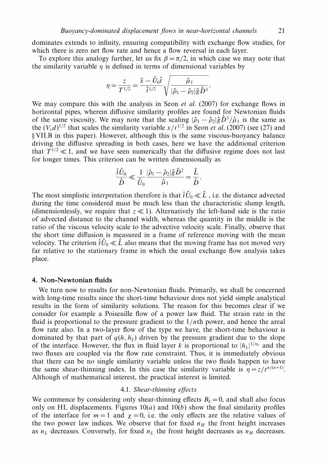
marks the limit where no static wall layers are possible. As nH decreases, the contoursbecome increasingly parallel to the vertical axis, which implies that the layer thicknessis becoming independent of B1 =BH/κH . As ϕb increases from negative to positivethe static layer thickness is increasing.

The limit BH → 0 must be treated separately. Straightforwardly, we find that Ystatic

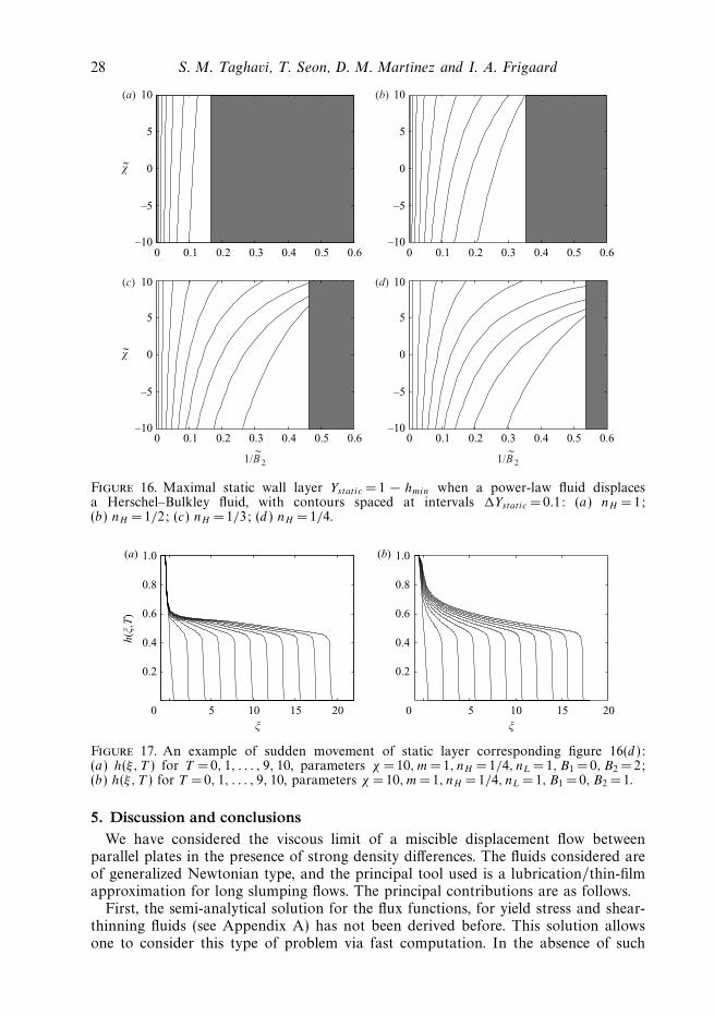
depends on nH , χ =χ/κH and B2 = BL/κH . Figure 16 shows the variation in maximumstatic wall layer with the parameters χ and B for four different fixed values of thepower law index nH . An interesting consequence of figure 16 is that for a smallchange in, e.g. yield stress, it appears that we may transition from having no staticlayer to having a finite static layer! An example illustration of this is given infigure 17. Although there is a discontinuity in the thickness of static layer, there isno discontinuity in the physical process, i.e. the layers of fluid that move do so veryslowly as the static layer criterion is violated.


0 0.1 0.2 0.3 0.4 0.5 0.6 0 0.1 0.2 0.3 0.4 0.5 0.6

0 0.1 0.2 0.3 0.4 0.5 0.6 0 0.1 0.2 0.3 0.4 0.5 0.6

0

–5

–10

5

10

0

–5

–10

5

10

χ~

0

–5

–10

5

10

0

–5

–10

5

10

χ~

1/B~

2 1/B~

2

(a) (b)

(c) (d)

Figure 16. Maximal static wall layer Ystatic = 1 − hmin when a power-law fluid displacesa Herschel–Bulkley fluid, with contours spaced at intervals �Ystatic = 0.1: (a) nH =1;(b) nH = 1/2; (c) nH = 1/3; (d ) nH = 1/4.

0 5 10 15 20

0.2

0.4

0.6

0.8

1.0

0.2

0.4

0.6

0.8

1.0

h(ξ,T

)

ξ

0 5 10 15 20

ξ

(a) (b)

Figure 17. An example of sudden movement of static layer corresponding figure 16(d ):(a) h(ξ, T ) for T =0, 1, . . . , 9, 10, parameters χ =10,m= 1, nH = 1/4, nL = 1, B1 = 0, B2 = 2;(b) h(ξ, T ) for T = 0, 1, . . . , 9, 10, parameters χ = 10,m= 1, nH =1/4, nL = 1, B1 = 0, B2 = 1.

5. Discussion and conclusionsWe have considered the viscous limit of a miscible displacement flow between

parallel plates in the presence of strong density differences. The fluids considered areof generalized Newtonian type, and the principal tool used is a lubrication/thin-filmapproximation for long slumping flows. The principal contributions are as follows.

First, the semi-analytical solution for the flux functions, for yield stress and shear-thinning fluids (see Appendix A) has not been derived before. This solution allowsone to consider this type of problem via fast computation. In the absence of such


a solution, to compute a solution requires numerical integration across the channelwidth in each fluid layer, coupled to iteration for the pressure gradients and stresses.In place we have simply to solve two coupled algebraic equations, both of which aremonotone in their argument. This is a considerable step forwards.

We have analysed principally the long-time behaviour of displacement flows.Although these are termed ‘long-time’ solutions we have seen in most of our computedexamples that the transients converge to something close to the long-time solutionsover time intervals T ∼ O(1). These flows are characterized by intervals of interfacethat propagate at a constant speed (fronts), and other intervals in which the interfacebecomes progressively stretched. The front heights are determined by considerationof the associated hyperbolic problem and it appears that the long time solutionconverges to a similarity form h(ξ/T ).

A range of parametric results have been reported in which we explore variationsin front heights and velocities with the model parameters. It is certainly fair to saythat some of the results are predictable, e.g. more efficient displacements are generallyfound with a more viscous displacing fluid and some modest improvements canalso be gained with slight positive inclination of the channel in the direction of thedensity difference. However, the value of the analysis really comes from quantifyingthe displacements, in terms of front heights and speeds, and in particular in helpingto determine efficiency in cases where physical effects are ambiguous (figure 10c).

Probably the most impressive improvements in displacement efficiency arise whenthe displaced fluid is significantly shear-thinning, by comparison with the displacingfluid (figure 10d ). Introduction of a yield stress can help displacements by makingthe displacing fluid more viscous, but if the displaced fluid has a yield stress it is verycommon to find completely static residual wall layers of displaced fluid. These areby-passed by the advancing front. Their thickness corresponds to the maximal staticlayer thickness and this can be computed directly, as we have done.

The key theoretical result is to establish that there can be no 100 % efficientdisplacements in this flow, regardless of rheological properties of the fluids (seeLemma 3 in § 2.4). A consequence of this is that we can focus in two directions:

(a) For the lubrication/thin film flows that we study, we may investigate whichrheological properties give the most efficient displacements and try more generally tounderstand the qualitative behaviour of solutions to the lubrication/thin film model.This has been the focus of the present paper.

(b) We may target attention at situations in which the underlying modelassumptions break down, e.g. due to flow instabilities developing or to otherphenomena that are discounted a priori in this type of model. This is where ourongoing research is directed.

In the above context, there are a number of model assumptions that meritdiscussion. First, let us emphasize that in lubrication/thin-film models there is alwaysan underlying assumption about the interface configuration, i.e. here we have assumedthat the slumping configurations of figure 2 are found for HL and LH displacements.For isodensity displacements we typically have a symmetric finger-like front advancingin the channel centre and there is no effect of interface slope or channel inclination.However, for small density differences both effects are present and we may expect thesymmetry to be broken, with the interface moving progressively towards this slumpingconfiguration. There is no inherent difficulty in modelling asymmetric finger-like frontswithin the thin-film framework. The transition between a slumping and finger-likedisplacement has not been studied, to our knowledge, and it is not clear to us how onewould proceed to deduce the transition between interface configurations purely from


this type of model. An interesting paper in this context is Shariata et al. (2004), whichillustrates that the resulting model systems can give rise to more complex behaviourthan that considered here. In the experimental context, in the miscible fluid exchangeflows of Seon et al. (2004, 2005, 2006, 2007), the interface is predominantly of theform of figure 2 when in the viscous regime, at near-horizontal inclinations. However,these experiments are conducted in a pipe and not a plane channel. Additionally,these experiments have no mean flow, so that no finger would be expected.

We note that although the result of Lemma 3 is established via a local analysis, ash ∼ 1, and results essentially from the no-slip condition at the upper wall, the no-slipcondition on its own does not imply that the interface can not propagate at steadyspeed along a wall. Indeed we have seen that this occurs at the lower wall at longtimes, for all parameters. More precisely, there is nothing mathematically present inthe form of the lubrication model to prevent steady interface propagation. Indeed, anexample of this occurs in Carrasco-Teja et al. (2008), where a Hele-Shaw displacementalong a narrow concentric annulus is considered. Instead it is the algebraic form of q

which distinguishes whether or not motion at the boundaries occur. Certainly, withslip at the upper wall we could achieve a steady displacement. This is the limitingcase of nL → 0 for the shear-thinning study in figure 10(d ). In Carrasco-Teja et al.(2008), symmetry conditions are imposed at the boundaries, which allows q to adopta suitable algebraic form for steady-state propagation.

A related question concerns whether or not the scaling assumptions leading tothe lubrication model may break down in the vicinity of the interface. In a strictlyhyperbolic model (i.e. of the same algebraic form as we have, with q = q(h, χ)), themoving front becomes a kinematic shock and the scaling assumptions break down.The kinematic and mass conservation equations are still valid, but the specification ofthe flux as a function only of the interface height becomes false. In our case howeverwe have seen, e.g. in figure 7(b), that the interface is smooth and the frontal section ofthe interface has finite width in ξ . Thus, there is no reason for the scaling assumptionsto become invalid.

A further interesting question concerns the stretched layer at the top of the channel(in an HL displacement). We note that the upper contact point of the interfacedoes not move (unless we have backflow), and thus at long times we are left with aprogressively thinning layer. We have seen that convergence to the long-time similarityprofile typically occurs on a time scale T ∼ O(1). As the layer thins progressively, wemay expect diffusive effects to become significant over a thickness [T/(δP e)]1/2 andcould use the final similarity profile h(ξ/T ) to estimate evolution along the channelof the distance where diffusion is significant, i.e. effectively matching:

[T/(δ Pe)]1/2 = 1 − h(ξ/T ).

There are other interesting questions in this same direction, e.g. estimating dispersivecharacteristics of miscible displacement flows, in the spirit of Taylor dispersion. Weleave these for future consideration.

This research has been carried out at the University of British Columbia, supportedfinancially by NSERC and Schlumberger through CRD project 354716-07. T. Seonalso acknowledges additional financial support from the Pacific Institute for theMathematical Sciences through a post-doctoral fellowship. This support is gratefullyacknowledged. We thank the reviewers for their suggestions which have helpedimprove the paper.


Appendix A. Computing the flux function q(h, hξ )

We address here the practicality of how to efficiently compute q(h, hξ ) for thenon-Newtonian fluid types that we consider. Since q(h, hξ ) is defined in terms ofu = u(y, h, hξ ), the first question is whether we may always find a velocity solution.The answer is yes, and we outline this later in § A.1.

For fixed h and ∂h/∂ξ , (2.18) and (2.19) for an HL displacement are

∂

∂yτH,ξy = −f, y ∈ (0, h), (A 1)

∂

∂yτL,ξy = b − f, y ∈ (h, 1), (A 2)

where f = −∂P0/∂ξ and with b = χ − hξ . Note that b physically represents thebuoyancy forces that drive the flow, being divided into two components: χ , whichrepresents the effects of the slope of the channel, and hξ , which represents the effectsof the interface slope. Thus, the shear stresses are linear in y in each layer.

We denote the wall shear stresses in heavy and light fluid layers by τH & τL,respectively, which may be defined in terms of the pressure gradient −f and interfacialstress τi as follows:

τH = τi + f h, (A 3)

τL = τi + (1 − h)(b − f ). (A 4)

In terms of τi , τH and τL the shear stresses in each layer are

τH,ξy(y) = τH

(1 − y

h

)+ τi

y

h, (A 5)

τL,ξy(y) = τL

h − y

h − 1+ τi

1 − y

1 − h. (A 6)

Using the constitutive laws of the two fluids, the velocity gradient u′(y) is now definedat each point in the two fluid layers. We now integrate u′(y) away from the wallsat y = 0 and y = 1 (where the no-slip conditions are satisfied) towards the interface.Depending on the choices of τH , τL and τi , and the rheological parameters of eachfluid, this leads to two interface velocities:

ui(h−) =

∫ h

0

u′(y; τH , τi) dy, (A 7)

ui(h+) =

∫ h

1

u′(y; τL, τi) dy, (A 8)

which need not be the same. For given wall stresses (τH , τL), we now iterate on τi ,until

�ui(τi) ≡ ui(h−) − ui(h

+) = 0. (A 9)

To make this procedure more clear, suppose that we have f fixed. For any givenτi , the wall stresses (τH , τL) are defined by (A 3) and (A 4). As τi increases, both τH

and τL increase. As the stress is linear in each layer and the constitutive laws aremonotonic, this means that the velocity gradients in (A 7) and (A 8) increase withτi and therefore we see that �ui(τi) increases monotonically with τi . Therefore (A 9)always has a unique solution (this could in fact be stated more formally and proven).Thus, for given f we are able to determine all of τH , τL and τi by imposing continuityof the velocity at the interface and using (A 3) and (A 4). For Herschel–Bulkley fluids


we are in fact able to give an analytical expression for the interface velocities in termsof the wall and interfacial stresses:

ui(h−) = h

⎧⎪⎪⎪⎪⎪⎨⎪⎪⎪⎪⎪⎩

[H (|τi | − BH )(|τi | − BH )mH +1 − H (|τH | − BH )(|τH | − BH )mH +1]

κmH

H (mH + 1)(τi − τH )τi �= τH

sgn(τi)H (|τi | − BH )(|τi | − BH )mH

κmH

H (mH + 1)τi = τH

,

(A 10)

ui(h+) = (h − 1)

⎧⎪⎪⎪⎪⎪⎨⎪⎪⎪⎪⎪⎩

[H (|τi | − BL)(|τi | − BL)mL+1 − H (|τL| − BL)(|τL| − BL)mL+1]

κmL

L (mL + 1)(τi − τL)τi �= τL

sgn(τi)H (|τi | − BL)(|τi | − BL)mL

κmL

L (mL + 1)τi = τL

,

(A 11)

where H (x) is the usual Heavyside function. Note that mk =1/nk . Thus, the iterationto find the solution of (A 9) involves simply a single monotone algebraic expression.

Having determined interfacial stress τi , we now integrate u(y) across each layer togive the flow rates in each layer, which are thus determined as a function of f and b:

qH =

⎧⎪⎪⎪⎪⎪⎪⎪⎪⎪⎪⎪⎨⎪⎪⎪⎪⎪⎪⎪⎪⎪⎪⎪⎩

hui(h+) − h2

κmH

H (τi − τH )2

{sgn(τH )H (|τH | − BH )

(|τH | − BH )mH +2

(mH + 1)(mH + 2)

+ sgn(τi)H (|τi | − BH )(|τi | − BH )mH +1

[BH − sgn(τi)τH

mH + 1+

|τi | − BH

mH + 2

]}τi �= τH

hui(h+) − h2

2κmH

H

sgn(τi)H (|τi | − BH )(|τi | − BH )mH

τi = τH

,(A 12)

qL =

⎧⎪⎪⎪⎪⎪⎪⎪⎪⎪⎪⎪⎨⎪⎪⎪⎪⎪⎪⎪⎪⎪⎪⎪⎩

(1 − h)ui(h−) +

(1 − h)2

κmL

L (τi − τL)2

{sgn(τL)H (|τL| − BL)

(|τL| − BL)mL+2

(mL + 1)(mL + 2)

+ sgn(τi)H (|τi | − BL)(|τi | − BL)mL+1

[BL − sgn(τi)τL

mL + 1+

|τi | − BL

mL + 2

]}τi �= τL

(1 − h)ui(h−) +

(1 − h)2

2κmL

L

sgn(τi)H (|τi | − BL)(|τi | − BL)mL

τi = τL

. (A 13)

The sum of the two flow rates gives the total flow rate. As argued above, and alsoproven in § A.1, we can show that the total flow rate increases with f . Consequentlywe may use any flow rate constraint to find f , via iteration. The equation for thefrictional pressure drop f is then

qH + qL = 1, (A 14)

which is again a single monotone algebraic equation. Finally, we have the solution:

q(h, hξ ) = qH ,∂P0

∂ξ= −f.


Computationally, the interfacial stress and modified pressure gradient are found viaa nested iteration, i.e. for fixed f we find τi in an inner iteration and then find f in anouter iteration. The inner iteration for τi finds a zero of (A 9). On physical groundswe should expect that the interfacial stress lies somewhere between the wall stressesfor each of the fluid phases. This allows us to prescribe upper and lower bounds forτi for the iteration. The iteration for f is based on solving the flow rate constraint(A 14). On physical grounds, we might expect the pressure gradient for the stratifiedflow to lie between the pressure gradients required to pump the same flow rate ofeither pure fluid. This is however not the case where there are extreme differencesin rheology and a significant density difference. Thus, instead we determine initialbounds for f numerically.

A.1. Existence of a velocity solution

Following the steps in Frigaard, Leimgruber & Scherzer (2003), for any f and b, forfixed rheological constants and h we may write the problem for finding the velocityu(y) as the following variational inequality:

a(u, v − u) + j (v) − j (u) � f QH (v − u) + (f − b)QL(v − u),

u ∈ W 1,1+n∗

0 (Ω), ∀v ∈ W 1,1+n∗

0 (Ω), (A 15)

where

a(u, v) = aH (u, v) + aL(u, v)

= κH

∫ h

0

|uy |nH −1uyvydy + κL

∫ 1

h

|uy |nL−1uyvy dy, (A 16)

j (v) = jH (v) + jL(v) = BH

∫ h

0

|vy | dy + BL

∫ 1

h

|vy | dy, (A 17)

QH (v) =

∫ h

0

v dy, QL(v) =

∫ 1

h

v dy, (A 18)

where n∗ = min{nH , nL} and W 1,1+n∗

0 (Ω) is a Sobolev space (see Hirsch & Lacombe1999) defined on Ω = [0, 1] containing functions that are zero at y = 0, 1, in theappropriate sense. Using standard theory from convex analysis (see, e.g. Ekeland &Temam 1976), this type of variational inequality has a unique solution u.

For given f we shall denote the solution by uf . We now consider two solutionsuf1

and uf2, corresponding to f1 �= f2. Treating uf1

as a test function for uf2and vice

versa, we insert into (A 15) and sum, to give

a(uf1, uf2

− uf1) + a(uf2

, uf1− uf2

) � [f1 − f2][QH (uf2− uf1

) + QL(uf2− uf1

)].(A 19)

Using the strict convexity of a(·, ·) (see, e.g. Ekeland & Temam 1976), it follows that

[f2 − f1][QH (uf2− uf1

) + QL(uf2− uf1

)] � 0. (A 20)

This inequality can be made strict provided that uf �= 0. Therefore, we see that thetotal flow rate QH + QL increases monotonically with f , and strictly monotonicallyprovided that uf �=0 (which may happen for given yield stresses). Consequently, thecriterion that

(QH + QL)(uf ) = 1, (A 21)

is sufficient to uniquely determine f . The rate of increase of the individual Qk withf can be estimated from the constitutive laws of the individual fluids. Monotonicity


of the flow rate with the applied pressure gradient is of course entirely intuitive fromthe physical perspective.

Appendix B. Monotonicity of q with respect to b

To demonstrate the monotonicity of q with respect to b, we use the variationalmethod above. For fixed b (and rheological constants), we denote by (ub, fb) thesolution (u, f ) to (A 15) that satisfies the flow rate constraint (A 21). Since (A 21) is

satisfied we may restrict the test space W 1,1+n∗

0 (Ω) to the subspace V ⊂ W 1,1+n∗

0 (Ω)such that (A 21) is satisfied for all v ∈ V . Consequently, (A 15) becomes

a(u, v − u) + j (v) − j (u) � −bQL(v − u), u ∈ V, ∀v ∈ V. (B 1)

We now consider two solutions ub1and ub2

, to (B 1), corresponding to b1 �= b2. Treatingub1

as a test function for ub2and vice versa, we follow the same steps as in the above

section for uf to arrive at

[b2 − b1]QL(ub2− ub1

) � 0. (B 2)

Thus, QL decreases with b and since q = 1 − QL we have that q increases with b.

REFERENCES

Allouche, M., Frigaard, I. A. & Sona, G. 2000 Static wall layers in the displacement of twovisco-plastic fluids in a plane channel. J. Fluid Mech. 424, 243–277.

Aris, R. 1956 On the dispersion of a solute in a fluid flowing through a tube. Proc. R. Soc. A 235,67–78.

Balmforth, N. J., Burbidge, A. S., Craster, R. V., Salzig, J. & Shen, A. 2000 Visco-plastic modelsof isothermal lava domes. J. Fluid Mech. 403, 37–65.

Balmforth, N. J., Craster, R. V. & Sassi, R. 2002 Shallow viscoplastic flow on an inclined plane.J. Fluid Mech. 470, 1–29.

Benjamin, T. J. 1968 Gravity currents and related phenomena. J. Fluid. Mech. 31, 209–248.

Birman, V. K., Battandier, B. A., Meiburg, E. & Linden, P. F. 2007 Lock-exchange flows insloping channels. J. Fluid Mech. 577, 53–77.

Carrasco-Teja, M., Frigaard, I. A., Seymour, B. R. & Storey, S. 2008 Visco-plastic fluiddisplacements in horizontal narrow eccentric annuli: stratification and travelling wavesolutions. J. Fluid Mech. 605, 293–327.

Chen, C.-Y. & Meiburg, E. 1996 Miscible displacements in capillary tubes. Part 2. Numericalsimulations. J. Fluid Mech. 326, 57–90.

Coussot, P. 1999 Saffman–Taylor instability in yield-stress fluids. J. Fluid Mech. 380, 363–376.

De Sousa, D. A., Soares, E. J., de Queiroz, R. S. & Thompson, R. L 2007 Numerical investigationon gas-displacement of a shear-thinning liquid and a visco-plastic material in capillary tubes.J. Non-Newton. Fluid Mech. 144 (2–3), 149–159.

Didden, N. & Maxworthy, T. 1982 The viscous spreading of plane and axisymmetric gravitycurrents. J. Fluid Mech. 121, 27–42.

Dimakopoulos, Y. & Tsamopoulos, J. 2003 Transient displacement of a viscoplastic material byair in straight and suddenly constricted tubes. J. Non-Newton. Fluid Mech. 112 (1), 43–75.

Dimakopoulos, Y. & Tsamopoulos, J. 2007 Transient displacement of Newtonian and viscoplasticliquids by air in complex tubes. J. Non-Newton. Fluid Mech. 142 (1–3), 162–182.

Ekeland, I. & Temam, R. 1976 Convex Analysis and Variational Problems . North-Holland.

Frigaard, I. A., Leimgruber, S. & Scherzer, O. 2003 Variational methods and maximal residualwall layers. J. Fluid Mech. 483, 37–65.

Frigaard, I. A., Scherzer, O. & Sona, G. 2001 Uniqueness and non-uniqueness in the steadydisplacement of two viscoplastic fluids. ZAMM 81 (2), 99–118.


Gabard, C. 2001 Etude de la stabilite de films liquides sur les parois d’une conduite verticale lorsde l’ecoulement de fluides miscibles non-Newtoniens. PhD thesis, These de l’Universite Pierreet Marie Curie, Orsay, France.

Gabard, C. & Hulin, J.-P. 2003 Miscible displacements of non-Newtonian fluids in a vertical tube.Eur. Phys. J. E 11, 231–241.

Griffiths, R. W. 2000 The dynamics of lava flows. Annu. Rev. Fluid Mech. 32, 477–518.

Hirsch, F. & Lacombe, G. 1999 Elements of Functional Analysis . Springer.

Huppert, H. E. 1982 The propagation of two-dimensional and axisymmetric viscous gravity currentsover a rigid horizontal surface. J. Fluid Mech. 121, 43–58.

Joseph, D. D. & Renardy, Y. Y. 1993 Fundamentals of two-fluid dynamics. Part 2. Lubricatedtransport, drops and miscible liquids. In Interdisciplinary Applied Mathematics Series, vol. 4.Springer.

Kondic, L., Palffy-Muhoray, P. & Shelley, M. J. 1996 Models of non-newtonian Hele-Shaw flow.Phys. Rev. E 54 (5), 4536–4539.

Lajeunesse, E., Martin, J., Rakotomalala N. & Salin, D. 1997 Three-dimensional instability ofmiscible displacements in a Hele-Shaw cell. Phys. Rev. Lett . 79, 5254–5257.

Lajeunesse, E., Martin, J., Rakotomalala, N. & Salin, D. 2001 The threshold of the instabilityin miscible displacements in a Hele-Shaw cell at high rates. Phys. Rev. Lett. 13 (3), 799–801.

Lajeunesse, E., Martin, J., Rakotomalala, N., Salin, D. & Yortsos, Y. 1999 Miscible displacementin a Hele-Shaw cell at high rates. J. Fluid Mech. 398, 299–319.

Leal, G. 2007 Advanced Transport Phenomena: Fluid Mechanics and Convective Transport Processes .Cambridge University Press.

Lindner, A., Coussot, P. & Bonn, D. 2000 Viscous fingering in a yield stress fluid. Phys. Rev. Lett.85, 314–317.

Nelson, E. B. 1990 Well Cementing . Schlumberger Educational Services.

Petitjeans, P. & Maxworthy, T. 1996 Miscible displacements in capillary tubes. Part 1. Experiments.J. Fluid Mech. 326, 37–56.

Rakotomalala, N., Salin, D. & Watzky, P. 1997 Miscible displacement between two parallelplates: BGK lattice gas simulations. J. Fluid Mech. 338, 277–297.

Sader, J. E., Chan, D. Y. C. & Hughes, B. D. 1994 Non-Newtonian effects on immiscible viscousfingering in a radial Hele-Shaw cell. Phys. Rev. E 49 (1), 420–432.

Seon, T., Hulin, J.-P., Salin, D., Perrin, B. & Hinch, E. J. 2004 Buoyant mixing of miscible fluidsin tilted tubes. Phys. Fluids 16 (12), L103–L106.

Seon, T., Hulin, J.-P., Salin, D., Perrin, B. & Hinch, E. J. 2005 Buoyancy driven miscible frontdynamics in tilted tubes. Phys. Fluids 17 (3), 031702.

Seon, T., Hulin, J.-P., Salin, D., Perrin, B. & Hinch, E. J. 2006 Laser-induced fluorescencemeasurements of buoyancy driven mixing in tilted tubes. Phys. Fluids 18 (4), 041701.

Seon, T., Znaien, J., Salin, D., Hulin, J.-P., Hinch, E. J. & Perrin, B. 2007 Transient buoyancy-driven front dynamics in nearly horizontal tubes. Phys. Fluids 19 (12), 123603.

Shariata, M., Talon, M., Martin, J., Rakotomalala, N., Salin, D. & Yortsos, Y. C. 2004 Fluiddisplacement between two parallel plates: a non-empirical model displaying change of typefrom hyperbolic to elliptic equations. J. Fluid. Mech. 519, 105–132.

Shin, J. O., Dalziel, S. B. & Linden, P. F. 2004 Gravity currents produced by lock exchange.J. Fluid. Mech. 521, 1–34.

Taylor, G. I. 1953 Dispersion of soluble matter in a solvent flowing slowly through a tube.Proc. R. Soc. A 219, 186–203.

Wilson, S. D. R. 1990 The Taylor–Saffman problem for a non-Newtonian liquid. J. Fluid Mech.220, 413–426.

Yang, Z. & Yortsos, Y. C. 1997 Asymptotic solutions of miscible displacements in geometries oflarge aspect ratio. Phys. Fluids 9 (2), 286–298.

Zhang, J. Y. & Frigaard, I. A. 2006 Dispersion effects in the miscible displacement of two fluidsin a duct of large aspect ratio. J. Fluid Mech. 549 (1), 225–251.

Buoyancy-dominated displacement ﬂows in near-horizontal ...

Documents

Transcript of Buoyancy-dominated displacement ﬂows in near-horizontal ...