Bundling with Customer Self-Selection: A Simple Approach to Bundling Low Marginal

Cost Goods

February, 2003

Lorin M. Hitt University of Pennsylvania, Wharton School

1300 Steinberg Hall-Dietrich Hall Philadelphia, PA 19104

lhitt@wharton.upenn.edu

Pei-Yu Chen Graduate School of Industrial Administration

Carnegie Mellon University 5000 Forbes Ave

Pittsburgh, PA 15213 pychen@andrew.cmu.edu

We would like to thank Ravi Aron, Erik Brynjolfsson, Eric Clemons, David Croson, Rachel Croson, Gerald Faulhaber, Steven Matthews, Moti Levi, Eli Snir, Raghu Srinivasan, Shinyi Wu, Dennis Yao and participants of the 1999 Workshop on Information Systems and Economics for helpful comments on earlier drafts of this paper.

2

Bundling with Customer Self-Selection: A Simple Approach to Bundling Low Marginal

Cost Goods

Abstract

The reduction in distribution costs of digital products has renewed interest in strategies for pricing goods with low marginal costs. In this paper, we evaluate the concept of customized bundling in which consumers can choose up to a quantity M of goods drawn from a larger pool of N different goods (N>M) for a fixed price. We show that the complex mixed bundle problem can be reduced to the customized bundle problem under some commonly used assumptions. We also show that, for a monopoly seller of low marginal cost goods, this mechanism outperforms individual selling (M=1) and pure bundling (M=N) when goods have a positive (even small) marginal cost, when users face costs of evaluating goods in the bundle, or when customers have heterogeneous preferences over goods. Comparative statics results also show that the optimal bundle size for customized bundling decreases in both heterogeneity of consumer preferences over goods and marginal costs of production. Altogether, our results suggest that customized bundling provides an efficient and mathematically tractable pricing scheme for selling information and other low-marginal cost goods, especially when consumers have heterogeneous preferences over goods or are budget or attention constrained.

1

1. Introduction

The emergence of the Internet as a low-cost, mass distribution medium has renewed interest in

pricing structures for information and other digital goods (Shapiro and Varian, 1998; Choi,

Stahl and Whinston, 1998). One common setting, faced by publishers, software producers,

music distributors, cable television operators and a wide variety of other firms, is when a

provider of a large number of information goods seeks to sell to a group of heterogeneous

consumers, who may place different values on the individual goods. While it is now possible to

efficiently sell individual goods separately for even small payments (Metcalfe, 1996), firms

may be able to generate greater profits by engaging in bundling, where large numbers of goods

are sold as a unit.

In theory, for N goods firms could offer up to (2N-1) possible bundles, each at a different price.

However, this problem is known to be computationally intractable and difficult to solve in

closed form except for small numbers of goods (Hanson and Martin, 1990). Recent work

(Bakos and Brynjolfsson, 1999) has shown that when the marginal costs of goods are

sufficiently low and customers share a common probability distribution for valuation of

different goods, pure bundling (offering all goods for a fixed price) is optimal, greatly

simplifying the bundling and pricing problem. However, less is known about situations where

it may be optimal to bundle large numbers of goods, yet marginal costs and consumer

preferences are such that pure bundling is inefficient. These types of situations arise when

goods have a small but non-negligible marginal cost (e.g., digital video distribution on a

congested network), when consumers value only a subset of all available goods (e.g., music,

movies, engineering software modules, past news articles), or when consumers face costs of

evaluating goods that increase in the number of goods offered in a bundle.

In this paper, we analyze a pricing approach which generalizes existing results on information

pricing while preserving simplicity and analytical tractability, which we term customized

bundling. A customized bundle is the right for a consumer to buy her choice of up to M goods

2

from a larger set N, for a fixed price p.1 Note that non-trivial customized bundling is only

relevant when marginal cost for each good is small and the goods share similar cost structure

otherwise, it will be more profitable to sell individual units. When consumer demand can be

characterized in a specific way, which is consistent with the assumptions used in some previous

work on information goods pricing, we show that the mixed bundling problem can be reduced

to a simple problem of non-linear pricing. This allows the application of known results to solve

otherwise very complicated bundling problems such as when individual sale can coexist with

pure bundling, when more than one bundle will be offered, how marginal cost affects the

optimal size of bundles, and the welfare effects of bundling. In addition, because customized

bundling contains unit sale and pure bundling as extreme cases, our analytical results can be

compared to and extend previous work on information goods bundling.

2. Previous Literature

The literature on bundling has a long history beginning with the observation by Stigler (1963)

that bundling can increase sellers’ profits when consumers’ reservation prices for two goods are

negatively correlated. In the two-goods case, offering both a two-good bundle as well as the

individual items (mixed bundling) is typically optimal (Adams and Yellen, 1976; McAfee,

McMillan and Whinston, 1989). This is because bundling reduces heterogeneity in consumer

valuations, enabling a monopolist to better price discriminate (Schmalensee, 1984; Salinger,

1995), while still capturing residual demand through unit sale. While the insight that bundling

reduces heterogeneity in valuations is quite general, other aspects of these solutions often do not

generalize beyond the two-good case.

Other work has extended the bundling literature to consider multiple goods as well as multiple

types. Spence (1980) generalized the principles of single product pricing problem to the case of

several products using a linear programming formulation, and shows some cases where the

1 Our definition is almost identical to “generalized bundling” studied by MacKie-Mason, Riveros and Gazzale (1999). This mechanism was also mentioned as a possible strategy for discriminating between customers with different willingness to pay (Bakos and Brynjolfsson, 1997; Shapiro and Varian, 1998), but this suggestion was not completely explored in previous work. The earliest reference to this approach of which we are aware is Chen (1997), who studied the properties of customized bundling using mixed integer programming, although variants of this scheme have been used in practice in software and music distribution for many years.

3

problem can be solved in closed form. Other tractable analytical solutions have been found for a

variety of special cases such as linear utility (McAfee and McMillan, 1988) or when valuations

across different consumers can be ordered in specific ways or satisfy certain separability

conditions (Armstrong, 1996; Sibley and Srinagesh, 1997; Armstrong and Rochet, 1999).

These papers have found additional general results such as the observation that it is usually

optimal to leave some consumers unserved in order to extract more revenue from the other

higher value consumers (Armstrong, 1996) and that it is sometimes optimal to induce a degree

of ‘bunching’, so that consumers with different tastes are forced to choose the same bundle of

products (Rochet and Chone, 1998). These papers provide a general structure for solving quite

complicated bundling problems in closed form, although the complexity increases dramatically

as more goods are considered, making it difficult to extend them to large numbers bundling

problems.

However, when marginal costs are very low, it is often optimal to bundle all goods together

(Bakos and Brynjolfsson, 1999) which leads to a dramatic simplification of the bundling

problem. These “pure bundling” results are robust to any set of consumer preferences

generated by a common distribution function for the value of each good across all consumers.

However, when pure bundles are not optimal, such as when consumers are budget or attention

constrained or marginal costs are significant, this mechanism provides little guidance since

limiting the size of a bundle of this form creates substantial deadweight loss when customers

are heterogeneous.2

There have been several studies that have considered large numbers bundling problems in

specific contexts related to information goods pricing. These studies generally find that

engaging in a form of mixed bundling where a certain large bundle is offered along side

individual sale dominates either strategy alone (Chuang and Sirbu, 1999; Fishburn, Odlyzko

and Siders, 1997). In addition, these studies introduce the idea that allowing customers to self- 2 The insight behind this shortcoming is straightforward. Suppose there are a large number of consumers that have valuation for each of 10 goods drawn from the same distribution function. It is clear that if we offer a pure bundle, all consumers will obtain their most preferred goods, although not all will agree which ones they are. However if we are constrained such that we can only sell, say, a 5 good bundle, there are now 252 possible bundles that a consumer might want if they can only have 5 goods. If any single bundle among the 252 possible bundles is offered, as few as 1/252 of the customers will receive their highest valued goods, creating substantial deadweight loss. Only by offering every possible combination that consumers desire would this deadweight loss disappear.

4

select the goods in the bundle (rather than having them predesignated) can often improve

outcomes while maintaining simplicity in the pricing mechanism (Chen, 1997; Chuang and

Sirbu, 1999; Mackie-Mason, Riveros and Gazzale, 1999).

3. Model

3.1 Introduction

We will examine the optimal bundling and pricing problem for a monopolist that distributes N

different goods to consumers. We are interested in examining the profitability of customized

bundles for a monopolist, in which a consumer is allowed to choose up to M goods ( M N≤ )

for a single price p . In general, a monopolist may want to offer more than one customized

bundle when facing heterogeneous customers. For notational simplicity we will use

[0,1/ , 2 / ,...,1]m N N∈ to represent a fraction of the total number of goods available and

let ( )p m represent the price for a customized bundle of size M mN= . In addition, for a

function ( )f m we define the notation '( )f m as 1( ) ( )Nf m f m− − for 1Nm > to be consistent

with the discrete nature of m.

3.2. Multiproduct Nonlinear Pricing for Heterogeneous Consumers

We begin by defining a structure for the standard bundling problem in which customers demand

at most one unit of each good. Consumers purchase a bundle of goods 1,.., ,..,j Nx x x=< >x

(where the elements of x are binary variables, {0,1}, 1..jx j N∈ = representing the purchase or

non-purchase of a bundle component) over all N goods available. Consumers derive benefits

from these goods which leads to a willingness to pay (WTP) ( )W x , a weakly increasing

function in all components of x with W(0)=0. In general there will be more than one set of

consumer preferences over these goods. Let there be I distinct types of consumers indexed

[1,2,.. ]i I∈ with a unique willingness to pay function ( )iW x . The proportion of each consumer

type in the population is denoted by iα (where 1

1I

i

iα

=

=∑ ). If the price of a set of goods is ( )p x ,

5

we could write the net utility a consumer i obtains from consuming this bundle as:

( , ( )) ( ) ( )i iU p W p= −x x x x .3 We denote the cost of providing a vector of goods x as ( )C x

which is weakly increasing in all components of x . Using this notation, the general bundling

problem the monopolist faces is the determination of the set of bundles offered { }x and a set of

prices ( )p x solving the well known mixed bundle pricing problem with heterogeneous

consumers (Spence, 1980):

1

max [ ( ) ( )] . .

IR: ( ) ( ) 0 IC: ( ) ( ) ( ) ( ) ,

Ii i i

i

i i i

i i i i j j

p C s t

W p iW p W p i j i

α=

−

− ≥ ∀

− ≥ − ∀ ≠

∑ x x

x xx x x x

(1)

The first set of constraints, individual rationality (IR), guarantees that if a consumer chooses to

purchase a bundle, it provides non-negative surplus. In other words, the monopolist cannot

force a consumer to purchase the bundle. The second set of constraints, incentive compatibility

(IC), guarantees that a consumer segment receives at least as much surplus for purchasing the

bundle intended for them than they would for choosing another bundle. Implicit in this

assumption is that the monopolist cannot price discriminate by group – it must be in the

consumer’s self-interest to purchase their intended bundle. This formulation treats the problem

as a direct revelation mechanism where consumers reveal their “type” through their choice of

product, which will yield the profit maximizing solution for the monopolist, if such a solution

exists (Myerson, 1979). Note from this formulation that for I consumer groups and N products,

the monopolist must determine the optimal set of I bundle compositions and prices out of

2 1N − possibilities.

3 3. Customized Bundling

Our initial interest is in determining the conditions under which the full bundling problem can

be reduced to the much simpler customized bundling problem. Following the literature on

information goods pricing, we will assume that the cost structure of providing goods to

3 The assumptions on W guarantee that U obeys the normal properties of utility functions.

6

consumers depends only on the number and not on which goods provided, thus ( ) ( )C C m=x

where 1mN

= x 1i (where i denotes a vector dot product, and 1 is a vector of all 1’s). We

further assume that C is weakly increasing, with decreasing differences in m (that is, ( ) 0C m′ ≥

and ( ) 0C m′′ ≤ ). Note also that (0) 0C = , consistent with an additional assumption that the

monopolist has already sunk any fixed cost necessary to produce these goods. Given this cost

structure, we now examine what types of consumer preferences (utility or willingness-to-pay)

will yield an equivalence between the optimal bundling problem and the optimal customized

bundling problem.

Before establishing these results, it is useful to introduce some additional notation. Let ( )iw m

represent the most a consumer of type i is willing to pay for mN goods (formally,

1

( ) max ( ) . . N

i ik

k

w m W s t x mN=

= ≤∑x x ). Note that this implies that (0) 0, '( ) 0i iw w m= ≥ and

"( ) 0iw m i≤ ∀ . Although there can exist as many as I such functions,4 in general there will be

less than I because different preferences ( )W x can yield the same expression for w(m). We can

now formulate customized bundling problem as:

1max [ ( ) ( )] . .

IR: w ( ) ( ) 0 IC: w ( ) ( ) w ( ) ( ) ,

Ii i i

i

i i i

i i i i j i

p m C m s t

m p m im p m m p m i j i

α=

−

− ≥ ∀

− ≥ − ∀ ≠

∑ (2)

This problem is the well-known non-linear quantity discrimination pricing problem with

heterogeneous consumers (also known as second-degree price discrimination; see Tirole, 1988,

p. 148-154). In addition to the mathematical formulation being identical, customized bundling

is also intuitively similar to second-degree price discrimination as it accomplishes

discrimination among different groups through customer self-selection from a menu of

offerings. The key distinction is that the non-linear pricing problem generally refers to different

quantities of an identical good, while customized bundling refers to heterogeneous goods with

4 In the context of information goods, it is reasonable to assume that I, number of consumer types, is much smaller than N, i.e., number of information goods offered.

7

similar valuations. Note also that this problem is significantly simpler than the full mixed

bundling problem (given in (1)) as it only requires a selection of a maximum of I prices from a

total space of N possible customized bundles.

An interesting question to explore is when we can reduce the complex mixed bundling pricing

problem (1) to the much simpler customized bundling pricing problem (2). Clearly, the two

problems are equivalent if they yield the same optimal pricing solution. The conditions for this

to hold are presented in Result 1 (all proofs are shown in the Appendix).

Result 1: The optimal bundle price schedule { , ( )}i ip i∀x x , is equivalent to a customized bundling solution ( )p m m∀ iff for every pair of optimal bundles ,i jx x where i j=x 1 x 1i i ,

( ) ( )i jw m w m=

This result shows for every optimal bundling solution there is an equivalent customized

bundling solution as long as the willingness to pay function over customized bundles is the

same for all customers whose optimal regular bundle is the same size. While this condition

seems both abstract and rather restrictive, a surprising number of assumptions on consumer

preferences meet these conditions. Specifically, this will hold if all preferences over regular

bundles ( ( )W x ) have a common customized bundle representation (w(m)).

The simplest example of this condition is when heterogeneous preferences map to a single

willingness to pay in customized bundles. For instance, if there are two consumer groups

(i={1,2}) and three goods (N=3) and the marginal cost per good is 0.25, the following two sets

of values for each of the three goods satisfy this property: {0.1,0.4,1} for consumer 1 and

{1,0.4,0.1} for consumer 2. This yields a WTP over customized bundles for all consumers of

{1.5, 1.4, 1,0} for m={1, 2/3, 1/3,0} respectively, and the monopolist optimally offers a 2-good

customized bundle at a price of 1.4, yielding a profit of 0.9. Chuang and Sirbu (1999) and Fay

and MacKie-Mason (2001) considered a more general form of this relationship, representing

consumer WTP by a linear function over their rank ordered preferences that satisfies this

condition. We examine in detail a minor generalization of their formulation in Section 3.5.

8

Interestingly, when there are a large number of consumers whose valuation is drawn randomly

from the same distribution function, as is common in marketing choice models (e.g,, McFadden,

1974) and previous work on information good pricing (e.g., Bakos and Brynjolfsson, 1999), the

resulting distribution of preferences over goods ( )W x yields a common distribution of

preferences over customized bundles w(m). As shown in Result 2, the equivalence between

regular bundling and customized bundling holds in this setting quite generally, only requiring

that valuations of goods can be described by a common cumulative distribution function where

the expected absolute value of each good is finite, a common assumption in previous work.

Result 2: If each of a large number of individual consumer’s willingness to pay for a vector of goods [0,1]N∈x is given by a vector NR∈v drawn independently from a common distribution function with cdf ( )F v with finite expected absolute value for all goods, there exists a willingness to pay function for customized bundles common across consumers. This function is

given by :(1 )

( ) [ ]N

k Nk m N

w m E X= −

= ∑ where :i NX is the ith order statistic from ( )F v

Result 2 shows that to calculate consumers’ willingness to pay across customized bundles for

random distributions, one need only calculate :(1 )

( ) [ ]N

k Nk m N

w m E X= −

= ∑ . The expression inside

the expectation, a linear combination of order statistics, is a special case of a general class of

functions called L-estimates (see a survey in Rychlik, 1998). The fact will prove useful in later

results we derive for random valuations.

3.4 General Solutions

We now consider the general solution to the generalized bundling problem (2). To solve this

problem, it is common to impose some additional structure on the variation across consumers

known as the Spence-Mirrlees single crossing property. This assumption enables closed form

solutions and straightforward comparative statics results, and is commonly used in theoretical

work on non-linear pricing. Let a and b represent bundle sizes (different values of m), let

consumers be indexed by i and j, the single crossing property (SCP) holds if there exists an

ordering of consumers such that:

9

( ) ( )( ) ( ) ( ) ( ) ,

i j

i i j j

w a w aw a w b w a w b a b i j

>

− > − ∀ > >.

This implies that a “higher type” consumer (meaning higher value of i in this condition) places

a greater value on any given bundle than “lower type” consumers. For all subsequent discussion

assume that customer types i are ordered to satisfy this condition. In addition, given any two

bundles, there is a greater difference in valuation due to size for higher type consumers (or in

other words, increasing differences in type and bundle size). While this appears to be restrictive,

it is a common assumption in most models of this type, and simply rules out cases where the

orderings of consumer value change as the bundle size changes. Moreover, it is necessary for

any general characterization of the solution to this problem.

Let * *{ , }i im p denote the optimal offering of the monopolist when there are multiple customer

types, and ˆ ˆ{ , }i im p represent the bundle that would be offered to consumer type (i) if there were

no incentive compatibility constraints (that is, if they were the only consumer type being

served). Using standard results and proof techniques from the theory of non-linear pricing we

can show the following Result.

Result 3: A monopolist will offer a set of customized bundles that have the following

properties:

a) The lowest-type customer that is served is priced at their willingness to pay: * *( )i i ip w m=

b) The prices for all other bundles are determined to satisfy IC, and leave all consumers except

the lowest type with positive surplus (let mini be the lowest type that is served): * 1* * 1* *

min( ) ( ) ( )i i i i i i i ip p w m w m w m i i− −= + − < ∀ >

c) The highest type customer is always served at the size they would have received if they were

the only customer segment: * ˆI Im m=

d) All other customers receive bundles smaller than the bundle size they would have received if

they were the only customer segment. These sizes are the greatest values of

[0,1/ , 2 / ,...,1]m N N∈ that satisfy:

10

* 1 * *

1( ) '( ) ( ) '( ) ( ) '( )

I I Ij i i j i i j i

j i j i j iw m w m C m i Iα α α+

= = + =

− ≥ ∀ <∑ ∑ ∑

e) There, in general, may be a customer segment such that all customers below that segment are

not served (that is, *min min0 . . 0ii s t m for i i∃ > = < )

f) The optimal size of the customized bundle is weakly decreasing in marginal cost

Result 3 replicates some of the well known results on non-linear pricing with a small

modification to account for the discrete nature of m. First, there is generally one optimal bundle

per type of consumer if that segment is served at all. Second, not all consumers are served with

since under single crossing it is more profitable to extract additional surplus form the “higher”

types than have them cannibalized by bundles targeted to the lower types. Third, only the

highest type consumer is served at their socially optimal bundle size, the rest being weakly

lower to discourage high types consumers from consuming bundles targeted at the lower types.

Fourth, because the monopolist cannot perfectly price discriminate, all consumers except the

lowest types that are served earn some surplus, an information rent due to their hidden type.

Finally, a more subtle observation is that without extremely restrictive assumptions on cost and

preferences, prices will not be linear in bundle size (with or without a “fixed fee” component)

suggesting that in general the optimal solution will outperform a two-part tariff (a formal proof

of this is available from the authors). All of these are a direct consequence of customized

bundling being a well-behaved nonlinear pricing problem under our assumptions.

There are also some additional insights these results bring that are unique to the customized

bundling problem. First, if cost and willingness to pay are known for each customer segment

(whether it is deterministic or the expectation of a random valuation), it is a simple calculation

of complexity O(I) to determine the optimal price and bundle sizes that will be offered. This

contrasts with the intractable mixed bundling problem of a large number of goods. Second, in

this formulation Result 3f provides a simple but powerful result on the relationship between

customized bundling, single good selling and pure bundling – as the marginal cost per good

increases, there is a monotonic shift between in optimal bundling policy from pure bundling to

customized bundling to unit sale.

11

Customized bundling becomes increasingly desirable relative to pure bundling when consumers

bear additional marginal costs of consuming larger bundles, for instance, when consumer

attention is scarce and larger bundles require greater consumer attention to evaluate and identify

their preferred goods. Let ( )iZ m represent the cost a consumer of type i faces in evaluating a

bundle of size m. Assume that ( )iZ m is positive and weakly increasing in m with weakly

increasing differences ( '( ) 0 and "( ) 0i iZ m Z m≥ ≥ ). We find that under some mild assumptions,

the optimal bundle sizes are further reduced, making it more likely that customized bundling

dominates pure bundling as shown in Corollary 1 below:

Corollary 1: Under the assumptions above, if consumers face an additional (private) cost of evaluating a bundle then bundle size is weakly decreased and prices are strictly decreased compared to the situation of no evaluation costs if

1

1

'( ) '( ) (1 ) '( )i

i i iI

j

j i

Z m Z m Z m i Iα

α

+

= +

≤ < + ∀ <

∑. Moreover, this condition will always be

satisfied if ( ) ( )iZ m Z m i= ∀ . In other words, as long as evaluation costs are enough to matter in the optimal solution, and are

the same across consumers or at least do not increase too fast in consumer type, evaluation costs

will tend to yield a smaller optimal customized bundle (the weak inequality due to the discrete

nature of m requiring a certain level of evaluation cost before bundle size is affected).

Overall, we are able to use our formulation and slight modifications of standard results to derive

some interesting insights into large numbers bundling problems regarding the number of

optimal bundles, the relationship between pure bundling and customized bundling, the response

to marginal cost changes, welfare effects, and the tractability of the pricing algorithm. However,

these general results do not say much how customized bundling is affected by the nature of

consumer preferences over different goods, the existence of attention limits (a maximum

number of goods desired), or budget constraints. In the next two sections, we make some

specific assumptions about cost and preferences to enable us to study these relationships.

12

3.5. Bundling Under a Two-Parameter Preference Function

For this section, we build on results by Chuang and Sirbu (1999) (CS) by considering a problem

where different consumers can be described by a willingness to pay function that depends on

two parameters: an overall budget constraint or total willingness to pay (b) and the number of

goods they value positively (K). We denote k as the fraction of goods that consumers’ value

positively (that is KkN

= ). Consumers are assumed to have similar utility functions over a rank

ordering of goods, which in the CS model is assumed to be linear in the rank order of their

preferences. We generalize this case to allow other relationships by assuming ( ) ( )mw m b yk

= i ,

where y(.) captures customers’ relative valuations, or degree of preference, for different goods.5

Therefore we can write:

( )( , )

mm

m

mby p if m ku m p k

b p if m k

− ≤= − >

(3)

where y is such that (0) 0, (1) 1, ' 0, '' 0y y y y= = > ≤ over the domain [0,1] (recall that this is

consistent with '( ) 0 and "( ) 0w m w m≥ ≤ given our definition of w(m) and that y’ refers to a

difference, not a derivative, to account for the discrete nature of m).

For any common function y(·) and any set of parameters { , , }i i ib k α characterizing consumer

preferences that satisfies single crossing we can directly apply Result 3 to obtain the optimal

bundling solution.

To make this analysis concrete, however, we focus on a single consumer type and make some

functional form assumptions for preferences and costs (the multi-type case is also easily solved

under SCP, but adds little insight over the general single type case). Specifically, assume that

5 One can think y(t) as the proportion or fraction of total budget that a customer is willing to spend on the top t percent of the goods she positively values. Intuitively, y is an increasing and concave function of t.

13

there is a constant marginal cost (c) for all goods, ( )C m cmN= , and that relative valuation (y)

across goods can be described by a quadratic function with a parameter (a) capturing

customers’ preferences across different information goods. The quadratic formulation is,

perhaps, the simplest functional form assumption that enables us to examine the differences

between relatively uniform preferences over goods and preferences skewed toward a few high

value goods. Moreover, given the properties of the y function ( (0) 0, (1) 1, ' 0, '' 0y y y y= = > ≤ ),

quadratic functions provide a reasonably good local (and often global) approximation to

arbitrary functional forms for ( )y ⋅ while maintaining computational tractability. Thus we have:

2( ) (1 ) [0,1] [0,1]my t a t at where t and ak

= + − = ∈ ∈ (4)

By varying a, we can examine different conditions of valuation for a given consumer or

representative consumer across different goods. If a=1 then we have the CS assumptions

(linearly decreasing value in rank order). If a=0, the consumer values all goods equally.

Under this formulation we can compare the efficiency (ability to maximize social welfare) as

well as the profitability of different bundling schemes. In this example, pure bundling is a

trivial solution as long as the pure bundle is profitable (that is, (1) 0b C− > ). The monopolist

sets price to total value (p=b) and extracts all surplus, although not at minimum cost when

1k < so it is not efficient (the monopolist incurs marginal cost to offer goods that are not

consumed). The optimal price per good for individual sale ( ISP ) is found by maximizing profits

subject to a constraint that the marginal utility of customers gained by purchasing additional

units of the good is equated with the prices paid:

arg max ( ) . . '( )IS PP PmN C m s t w m PN= − =

The optimal customized bundling solution is just a special case of Result 3 where there is only

one type of customer. Because there is only one type, we can ignore incentive compatibility

and focus entirely on individual rationality. Thus the price for a customized bundle ( CBp ) is

given by:

14

arg max ( ) . . ( ) 0CB pp p C m s t w m p= − − ≥

Note that the constraint is always binding at the optimum, so we can rewrite the objective

function as:

arg max ( )CB mm w m cNm= −

This equation is identical to the problem of maximizing social welfare and, thus, there is no

deadweight loss, so the customized bundling solution is efficient.

We summarize the solutions and results to individual sale ( ,IS ISm π ), pure bundling ( ,PB PBm π )

and customized bundling ( ,CB CBm π ) in the following two graphs (detailed derivations appear in

the Appendix). For ease of comparison, we define bwkN

≡ to be the average willingness to pay

for the goods that have positive values. Figures 1a and 1b characterizes profit and bundle size

for various regions of marginal cost per good (c) and customer preference parameter over goods

(a). Note that since customized bundling contains both pure bundling and individual sale as

extreme cases, it will always weakly dominate. However, the degree of difference depends on

marginal cost and the dispersion of values across goods. As shown in Figure 1a, only when

marginal cost is zero is customized bundling and pure bundling equivalent in profits. This

continues up until marginal costs are equal to kw when pure bundling is no longer feasible

while customized bundling is still profitable. Finally at (1 )w a+ customized bundling is no

longer feasible. Altogether, these results suggest that the profitable region of customized

bundling expands as a increases (i.e., when there is increasing difference in good valuations).

15

Figure 1a: Pure bundling vs. customized bundling for different marginal cost and customer

preference parameter

Figure 1b: Individual selling vs. customized bundling for different marginal cost and customer

preference parameter

In Figure 1b, at very low marginal cost and low dispersion of valuation across goods

when ' (1 3 )C c w a= < − , individual selling and customized bundling are equivalent in number of

goods sold, which is the efficient solution. They also achieve the same profit level when a=0.

But as a departs from zero but is smaller than (1 3 )w a− , individual selling is efficient but not

c

(1 )c w a= +

kw

0CB PBπ π> =

0CB PBπ π≥ ≥

CB PB bπ π= =

a 1/3 2/3 1

w

2w

0 0

0CB PBπ π= =

c kw=

c

(1 )c w a= +

a 1/3 2/3 1

w

2w

0 0

(1 )c w a= −(1 3 )c w a= −

0

0IS CB

IS CB

m m

ππ= =

= =

0

0 2IS CB

IS CB IS

m m k

π π π

< < <

< < =

0

0IS CB

IS CB

m m k

b ckNπ π

< < =

< < = −IS CB

IS CB

m m k

b ckNπ π

=

≤ = −

=

16

profit maximizing. Note also that market demand (goods that are positively valued) can be fully

satisfied using customized bundling for a values three times as large as the case of individual

selling for the same level of marginal cost. Finally, as marginal costs increase, the size of

customized bundle decreases until marginal cost is so high that bundling is infeasible.

The key insight from this analysis is found from an examination of the “normal” case with non-

zero marginal costs and consumers placing different values over different goods (a>0). In this

case, customized bundling dominates the alternative approaches, even when there is only a

single customer segment (except in the boundary cases where they are equivalent, m k= 6 for

individual sale, and m=1 for pure bundling). In other words, as marginal costs (c) increase or

customer heterogeneity across goods (a) becomes larger, it is increasingly attractive to

consider customized bundling over the alternatives of pure bundling and individual sale. While

pure bundling is only feasible when average cost drops below average budget ( bc kwN

≤ = ),

customized expands the range of feasible bundling to include (1 )kw c w a≤ ≤ + , and

customized bundling is strictly better whenever there is heterogeneity in valuations (a>0) or

consumers do not value all goods (0<k<1). These analyses are illustrated in Figures 2a-2c (see

remaining figures at the end) showing the profitability of the various approaches for varying

levels of the parameters (c,a,b,k).

All of these results hold for a single group of customers. The contrast will only increase if we

allow multiple customer segments since customized bundling can offer tailored bundles to each

segment, a strategy not possible with individual sale or pure bundling without some

segmentation mechanism.

3.6. Customized Bundling Under Random Valuation

6 m represents total number of goods sold to each customer in the case of individual selling.

17

We earlier showed that simple customized bundling solutions may exist when consumers have

valuations for multiple goods drawn from a single valuation distribution.7 Since a number of

previous papers in information goods bundling have used such distributional assumptions

(especially Bakos and Brynjolfsson, 1999, referred to hereafter as BB), it may be useful to

compare the customized bundling solution to the pure bundling alternative under random

valuation drawn from a certain distribution. Unlike BB who considered the effects of changing

the number of goods in the population, we will consider a simplified structure compared to BB

in which N is fixed at the largest possible number of goods. It should be noted that once N is

fixed, pure bundling is a special case of customized bundling. We will retain the BB

assumptions of identically distributed iv (the value of the ith good) and their assumption of

constant marginal cost per good (which may be zero). In addition, all distributions considered

here are assumed to meet the conditions described in Result 2 (essentially finite expected

absolute value). For the following results, it is useful to define the “Quantile” or “Inverse

Distribution Function” of a distribution function F(t) as ( ) sup( : ( ) )FQ z t F t z= ≤ .

The most general result we can show for arbitrary distribution functions, including those where

valuation is dependent, is that customized bundling value is bounded below by mean valuation,

and above by an integral expression involving the quantile function:

Result 4: If the valuation for any individual good is drawn from a common but possibly

dependent distribution F(·) with finite mean (µ ) then 1

1( ) ( )Fm

Q z dz w m mNµ−

≥ ≥∫

There are two interesting insights from Result 4. First, the upper bound can sometimes serve as

a reasonable approximation for the value of customized bundling, as it can be interpreted as an

approximate average value of the portion of the distribution that exceeds the mth percentile.

Simulation results on many common distributions (uniform, normal, logistic and exponential)

suggest this approximation is good when the valuation of different goods is not too dependent.

Second, the result shows that the expected value of a customized bundle always (weakly)

7 This can be extended to multiple distributions as long as they generate willingness to pay functions that obey the single crossing condition. However, this formulation yields few incremental insights beyond the single type case discussed here and the general formulation in Result 3.

18

exceeds the mean value of the same number of goods, implying that average valuation per good

of customized bundles under most circumstances exceeds the average value of per good of pure

bundles. The strict lower bound only holds when m=1 or valuations of goods are perfectly

correlated.

With addition distributional assumptions we can apply the theory of L-estimates to obtain a

number of additional general results. The most straightforward exact results can be obtained

when we further assume independence of good valuations, that is 1

( ) ( )N

ii

F F v=

=∏v . This

assumption yields an explicit expression for ( )w m .

Result 5: If the valuation of individual goods is independently and identically distributed with

quantile function ( )FQ z then 1

:0

( ) ( ) ( )N

F i Ni mN

w m Q z N z dz=

= ∑∫ where 1:

1( ) (1 )

1i N i

i N

NN z N z z

i− −−

= − −

(the Bernstein Polynomials). This expression can be used to numerically calculate the values of the consumer willingness to

pay for arbitrary distribution functions and may be solvable in closed form for some

distributions such as the uniform and the exponential. It can also be applied to make

comparative statics predictions regarding distribution parameters such as mean or variance and

the size of the optimal customized bundle.

Because the customized bundling profit function ( ( ) ( ) ( )m w m C mπ = − ) has a direct

relationship with the quantile function, a number of useful results can be obtained restricting

our attention to distributions in the location-scale family, which includes most common

distributions assumed in prior work such as the exponential, normal and uniform. Location-

scale distributions are such that for a distribution with two parameters ( , )a b known, we can

write the quantile function as ( ; , ) ( ;0,1)F FQ z a b a bQ z= + where a is referred to as the location

and b as the scale. Using this definition and the usual assumption of a constant marginal cost

for each good (c), it is now possible to derive a relationship between location (proportional to

19

the mean) and scale (proportional to variance) for an arbitrary i.i.d. distribution in this family

and the optimal customized bundle size ( *m ).

Result 6: Let the valuation for any individual good be drawn i.i.d. from a distribution ( )F x

with mean (µ ), in the location-scale family with location a and scale b. Then:

a) *m is weakly increasing in a.

b) For general distributions *m is weakly increasing in b if 1:[ ]M NE X c+ < where M is

the lowest order statistic of the standard distribution for ( )F x (a=0, b=1) with non-

negative expected value. *m is weakly decreasing in b if 1:[ ]M NE X c− > .

c) Profits are always increasing in *m at optimum

For any fixed marginal cost, an increase in location simply shifts the valuation curve outward in

marginal value-size space, increasing optimal bundle size (unless the optimal bundle is already

the pure bundle). The intuition behind the scale is somewhat more complex. Note that as scale

(variance) increases, the distribution spreads out. The highest order statistics become larger and

the lowest order statistics become lower. If the optimum lies in a region where the order

statistics are increasing in variance (i.e., when 1:[ ]M Nc E X +> , that is, when c is relatively large

and the optimal bundle only includes the very highest valued goods), then increasing scale

raises the size of the bundle. If the optimum lies in a region where they are decreasing in scale

(that is, when c is relatively small), the optimal bundle size is decreasing in scale. The

conditions in 6b guarantee the location of this optimum and that this optimum doesn’t move to

the opposite side of the curve as scale is changed.

This result shows an interesting relationship between the pure bundling and customized

bundling. When it is feasible to have a pure bundling solution (the average value greater than

marginal cost), then greater variance will decrease the performance of pure bundling relative to

customized bundling because it means that the lowest valued goods in the bundle become even

worse with increasing variance and thus will make customized bundling more attractive. This

provides an additional reason why greater ex-ante uncertainty about consumer valuations makes

pure bundling less undesirable. The BB explanation is that it slows convergence of valuation to

20

the mean in finite samples which leaves consumers with more surplus. However, we add an

additional explanation that the goods being bundled on the margin under higher variance get

increasingly worse. We also show that increasing variance will decrease the size of customized

bundle when marginal cost is relatively small. Interestingly, however, in the region where pure

bundling is infeasible but there are still feasible customized bundles ( :[ ]N Nc E Xµ < < ) variance

actually leads to larger customized bundles and greater bundling profits in contrast to the BB

results for low marginal costs.

If we are willing to make stronger distribution assumptions, it is possible to relax the

independence assumption slightly. While in general it is difficult to calculate order statistics

from non-independent distributions, simple expressions exist for the multivariate normal with

common correlation ( )ρ . These results are given in Result 7, using the same notation

introduced in Result 6b:

Result 7: The optimal bundle size and total bundle profits are decreasing in the correlation

among goods when 1:[ ]M NE X c+ < , and increasing in correlation when 1:[ ]M NE X c− > where

M is the median.

This Result indicates that negative correlation acts similarly to variance, with negative

correlations raising the value of the highest valued goods, but also decreasing the value of the

lower valued goods. In the region where pure bundling is efficient we have another contrasting

result with BB – while negative correlation improves price discrimination ability of the

monopolist, it is offset by the fact that the lowest value goods are worth even less, reducing the

price discrimination gains of pure bundling and favoring customized bundles.

These analyses can be straightforwardly expanded to multiple consumer types provided that the

implied customized bundle valuations satisfy single crossing using Result 3 (or can be solved

by mixed integer programming when that is not true). However, this analysis does not yield

any additional insights beyond the individual contribution of Result 3 and the single-type results

in this section.

21

4. Summary and Conclusion

We have analyzed an alternative bundling mechanism for low marginal cost goods that allows a

consumer to choose up to M of their preferred goods from a larger set N for a fixed price p.

Comparing to traditional second-degree price discrimination, in which firms try to solve p(x)

over 2N-1 possibilities, customized bundling is much simpler in implementation when consumer

preferences are such that the optimal full bundling solution has an equivalent customized

bundling representation. We further show that these requirements are satisfied by assumptions

used in prior bundling work, especially when consumer valuations are drawn from an identical

valuation distribution across goods. Customized bundling yields a natural form of price

discrimination for heterogeneous consumers by offering a price-bundle size schedule that

includes individual sale and pure bundling as special cases.

Since customized bundling is simply an application of a well-behaved non-linear pricing

problem, it retains the properties of these problems including one type of offering per customer

segment, the “no distortion at the top” result that the highest valuation consumers receive their

optimal bundle, information rents to all but the lowest type consumers, and the possibility that

some of the lowest types are not served. In addition, customized bundles become optimal when

marginal costs are non-zero but not so large that the solution is individual selling. We also

demonstrate using specific representations of consumer preferences that customized bundling

can be advantageous when consumer preferences are concentrated on a few goods, consumers

have limited attention for evaluating goods in a bundle, or they have budget constraints (either

attention or financial). In addition, for the case when consumer valuations are generated by

common distributions we also show that uncertainty about consumers valuations (variance)

makes customized smaller bundles more attractive when marginal costs are low, but the optimal

customized bundle size increases in variance when marginal costs are high (in contrast to Bakos

and Brynjolfsson, 1999). However, unless marginal costs are zero and customers value all

goods, customized bundling will strictly dominate pure bundling.

22

The advantages of customized bundling are likely to be especially relevant when monopolists

are selling large numbers of high value goods (e.g., movies) since it is very likely that budget

constraints are binding and distribution costs are significant, at least using current technologies

or when customers have heterogeneous valuations over different goods and do not positively

value all goods. Other markets that have similar characteristics are high-quality digital music or

modular packaged software (Office suites, e-commerce platform software, or the SAP R/3

system, for example). For smaller numbers or lower value goods, it is likely that pure bundling

will prevail, at least if consumers are homogeneous in the ways considered in our model and

those of our predecessors. However, even in these cases, customer heterogeneity is likely to

create opportunities for offering different size of customized bundles, as it provides a greater

ability to target different segments than individual pricing or pure bundling, which must rely on

third-degree price discrimination to deal with residual customer differences.

Given these advantages while maintaining a relatively simple pricing structure, it is somewhat

surprising that these mechanisms are not already widespread. However, there is increasing

evidence that these types of mechanisms are being implemented or could be favourably

employed. In a field experiment MacKie-Mason, Riveros and Gazzale (1999) found that

librarians shifted toward purchasing journals through customized bundling (or “generalized

bundling” in their terminology) when this option was offered along with other more traditional

pricing schemes. Their consumption of customized bundles increased over time relative to

other pricing approaches, even when it was likely that preferences over journal articles was

largely unchanged. We have also identified a number of other examples used in practice.

Many firms offering engineering drawing software – a moderately expensive and modular

software package – offer modules in customized bundles (e.g., purchase a “10-pack” for $2000

or a 5-pack for $1250 where the consumer chooses from all available modules). There is also

the well known “10 CDs for a $1” promotions by firms such as Columbia House, which

represent the purchase of a customized bundle of around 14 CDs for approximately $75 (once

contractual requirements are met). At least one online movie rental club (netflix.com) currently

uses a customized bundling scheme – their pricing scheme allows users to choose different

plans that enable them to simultaneously borrow N videos for p(N) dollars per month where

multiple values of N are allowed (currently 2, 3,4, 5, and 8). The New York Times has

23

experimented with a bundle pricing scheme for access to their article archives with four pricing

options, with which the articles purchased are chosen by the consumer: 25 articles for $25.95,

10 articles for $15.95, four articles for $7.95 or a single article for $2.95.8 This suggests that

firms are exploring the use of these mechanisms, although it is likely that many of the domains

in which this is most relevant have not yet seen substantial experimentation in pricing structure.

While we have specifically focused our attention to information goods, customized bundling

technique is not unique to information goods, and it is especially attractive when number of

goods offered is large but marginal cost and valuations are such that it is optimal for consumers

to purchase more than one good. For example, some restaurants have traditionally “bundled” a

selection of two or three side dishes with a meal where consumers choose from a specified set.

More recently, McDonalds changed their menu from traditional second-degree price

discrimination with fixed bundles (“value meals” with a sandwich, french fries and drink) to an

arrangement where customers choose two side dishes form a list of items.

In addition to the potential for practical use, our customized bundling analysis provides another

simplification to the general problem of mixed bundling that may be appropriate in some

circumstances. Given the complexity of the general problem, there has been tremendous

interest in the marketing, management, computer science, and economics communities for

approaches that yield tractable analytic bundling solutions.

8 http://www.nytimes.com/premiumproducts/archive.html.

24

Appendix (Proofs): Proof of Result 1 (sufficiency). Starting the program described by (1), we show that it can be converted to the problem stated in (2). Consider any collection of consumers {i} where the optimal solution to (1) is { ix } s.t. i mN⋅ =x 1 for all members of this set. For every other value of m for this set of consumers, there must exist some x , with

mN=x 1i such that ( )iW x is maximized, thus ( )iw m and ( ) ( )i iW w m=x for this set of x . By the sufficient

condition, all consumers i in this set must be such that ( ) ( )iw m w m= . We now establish an equivalence

( ) ( )ip p m=x for all consumers in this set. If there is only one such element, there is a 1-1 mapping between ix

and im and thus ( ) ( )i ip p m=x for that value of m. If there are two or more, then choose any two arbitrarily,

labeling them kx and lx . For both of these bundles, either IR or IC must bind, otherwise ( )p i is unbounded. Changing variables in the willingness to pay functions from x to m and applying the assumed condition we can rewrite the constraints as: ( ) ( ) 0kw m p− ≥x , ( ) ( ) 0lw m p− ≥x and

( ) ( ) ( / ) ( )k j jw m p w N p j− ≥ ⋅ − ∀x x 1 x and ( ) ( ) ( / ) ( )l j jw m p w N p j− ≥ ⋅ − ∀x x 1 x . There are 4 possible cases, both IR are binding, both IC, and two cases where 1 IR and 1 IC binds. If IR is binding for both then it immediately follows that: ( ) ( ) ( )j lp p p m= =x x . If both IC bind, then it must bind at some value j for

which ( / ) ( )j jw N p⋅ −x 1 x is maximized. This value (call it Q) does not depend on k or l. Thus if both IC

constraints hold, ( ) ( ) ( ) ( )l kw m p w m p Q− = − =x x or ( ) ( ) ( )j lp p p m= =x x . The case where 1 IC binds and 1 IR binds cannot be an optimum since it implies that Q must be both greater than and less than zero. This establishes that , ii mN∀ ⋅ =x 1 , ( ) ( )ip p m=x . Substituting for ( ), ( ), ( )i i iw m C m p m for

( ), ( )i iC px x and deleting redundant constraints we obtain the customized bundling problem shown in (2) (necessity). Given an optimal customized bundling schedule ( )p m m∀ , suppose that there exists two bundles

kx and lx for some m where i mN⋅ =x 1 where ( ) ( )j lp p>x x . From the same type of argument shown

above, if at least 1 constraint (IR, IC) must be binding for each, this implies that ( ) ( )i j i lW W>x x which

contradicts the condition ( ) ( ) ( )k k l lW W w m= =x x . Proof of Result 2: (by construction) Proof (by construction). Let the ith order statistic of the valuation of N goods given by ( )F v be denoted as :i NX (where the largest order statistic is given by :N NX ). The random willingness

to pay for any consumer is :( )N

k Nk mN

w m X=

= ∑ . This function does not depend on the consumer examined

(equivalence). For any given distribution there exists a distribution for each order statistic and summation is a Borel measurable function. Therefore, there exists a cdf for ( )w m for each m (existence). Finally, we know

[| ( ) |]E w m < ∞ since : :1

[| ( ) |] [ | |] [ | |]N N

i N i Ni mN i

E w m E X E X= =

= ≤ < ∞∑ ∑ . Across each consumer, ( )w m is

independent and identically distributed with finite mean (since [ ( )] [| ( ) |]E w m E w m≤ < ∞ ). Therefore, letting

Q represent the number of customers, average valuation 1

1 ( ) [ ( )]Q

iw m E w m

Q =

→∑ as Q →∞ by the Strong

Law of Large Numbers.

25

Proof of Result 3: The maximization program is given by:

Max 1

( )n

i i i

i

P C mα=

⋅ − ∑

s.t.

: ( ): ( ) ( ) 2.. ,: ( ) ( ) 1.. ,[0,1/ , 2 / ,...,1]

i i i

i i i j i i

i i i i j j

i

IR w m p iDIC w m p w m p for i I and j iUIC w m p w m p for i I and i j Im N N i

≥ ∀

− ≥ − = ∀ <

− ≥ − = ∀ < <

∈ ∀

Assume initially that all types can be profitably served in this market by an ordering of bundles

1* 2* *Im m m≤ ≤ ≤ ). We can show that only adjacent DIC constraints can bind. Define the adjacent incentive compatibility constraints to be

1 1( ) ( ) 2i i i i i iw m p w m p i− −− ≥ − ∀ ≥ Now we will show that if the adjacent incentive compatibility constraints hold, then all the incentive compatibility constraints hold. Consider any j<i-1;

1 11 1( ) ( ) [ ( ) ( )] [ ]

i ii i i j i k i k k k i j

k j k j

w m w m w m w m p p p p− −

+ +

= =

− = − ≥ − = −∑ ∑

or equivalently, ( ) ( )i i i i j jw m p w m p− ≥ − As a result, DIC can be replaced by the adjacent incentive compatibility constraints. After these simplifications, the original problem is equivalent to the following problem, ignoring UIC:

Max 1

( )n

i i i

i

P C mα=

⋅ − ∑

s.t.

1 1 1

1 1

( )( ) ( ) 1

[0,1/ , 2 / ,...,1]

i i i i i i

i

w m pw m p w m p im N N i

− −

≥

− = − ∀ ≥

∈ ∀

By substituting in all the IC constraints (which generates a recursive equation that gives all prices in terms of willingness to pay) and collecting the terms together for each mi we can see that the IC constraints include a term for ( )i iw m for all prices in sequence above ip and 1( )i iw m+ for all prices in the sequence of prices above 1ip + .

Therefore and taking derivatives for each im yields

* 1 * *1'( ) '( ) '( )i i i i i i

i iI

ji

j i

w m w m C m i I

where

α α α

α α

++

=

− = ∀ <

=∑ (C1)

and at i=I, * *[ '( ) '( )] 0I I I Iw m C mα − = , because there is no group above them to have an IC constraint. Therefore, the highest type purchases the efficient optimal bundle size. Two final issues arise – what is the lowest group served and what happens when (C1) cannot be satisfied for a positive mi. An approach is to compute the entire sequence of mi that arise from the program above. Whenever monotonicity is violated in the mi, say

* 1*x xm m −< , a more profitable strategy is to pool type x and type x-1, that is set * ( 1)*x xm m −= . Note that this action does not alter any other constraints, namely IR and IC constraints we have, in particular, the relevant IC constraint to ith group, * 1* * 1* 1* 1* 1* 1*( ) ( ) ( ) ( )i i i i i i i i i i i ip p w m w m p w m w m p− − − − − −= + − = + − = , is still

26

satisfied. (*) By inspecting the sequence of optimal sizes to the program, we could identify the relatively unprofitable groups, those with optimal size smaller than that of their adjacent lower types, and then we pool these relatively unprofitable types to their adjacent lower types and relabel the segments and adjust the size of each segment, note that by doing this the number of bundles (prices and sizes) we have to determine is reduced. Calculate the solution to this modified problem, if monotonicity is satisfied, then the solution is an optimal one; if not, we run (*) again until monotonicity is satisfied. Proof of Corollary 1: Substitute ( ) ( )i i i iw m Z m− for ( )i iw m in the proof of Result 1. The quantity reduction arises from condition in Result 1d combined with the condition on Z’ above which yields a relationship of marginal revenue is less than marginal cost and thus a quantity reduction. The last expression follows directly from the fact that iα is positive. Proof of Result 4. Using Rychlik (1999, p. 108, eq. 11) we have that the trimmed mean of a set of random variables has tightest bounds (for a general distribution):

/ 1

:0 ( 1) /

1( ) ( )1 1

k n k

F i n Fi j j n

k nQ z dz E X Q z dzn k j n j= −

≤ ≥+ − + −∑∫ ∫ . Substituting

, 1,n N j N mN k N= = − + = yields 1 1

:0 1

1( ) ( )N

F i n Fi mN m

NQ z dz E X Q z dzmN mN= −

≤ ≤∑∫ ∫ . Multiplying both

sizes by mN and applying the definition of expected WTP yields the result.

Proof of Result 5: For i.i.d random variables, 1

: :01 1

( ) ( )N N

i i N F i i Ni i

E c X Q z c N z dz= =

=∑ ∑∫ where :i NX is the ith

(highest) order statistic from a sample of size N. If 01i

i mNc

i mN<

= ≥ then the first term in the expression

becomes : [ ( )]N

i i Ni mN

E c X E w m=

=∑ and the right hand term becomes the expression shown above.

Proof of Result 6: Denote the solution to the monopolists problem max ( ) max ( ) ( )m mm w m C mπ = − as

*m . From Result 4, 1

:0

( ) [ ( ;0,1)] ( )N

F i Ni mN

w m a bQ z N z dz=

= + ∑∫ . The range of possible values

( , , )a b m forms a lattice ( 2 [0,1/ ...,1]N× ). Therefore comparative statics on the parameters can be examined

using Topkis’ theorem (Topkis, 1978). Denote 1m mN− = − . From Topkis’ theorem, we know that *m is

increasing in ζ if ( )( ) 0mm ππ

ζ ζ−∂∂

− ≥∂ ∂

. Writing 1

:0

( ) ( ) [ ( ;0,1)] ( )F mN Nw m w m a bQ z N z dz−− = +∫ . For

comparative statics on a we have 1

:0

( )( ) [ ( ) ( ) ] ( ) 0mN Nmm w m w m c N z dz

a a aππ −

−

∂∂ ∂− = − − = >

∂ ∂ ∂ ∫ (the

Bernstein polynomials are all positive) so *m is increasing in a. For comparative statics on b the derivative of

the difference reduces to: 1 1

: :0 0

[ ( ;0,1)] ( ) ( ;0,1) ( )F mN N F mN Na bQ z N z dz Q z N z dzb∂

+ =∂ ∫ ∫ . This is just a mN

order statistic from a standardized distribution. Define M as the lowest order statistic of the standard distribution

27

with non-negative expected value. The comparative statics w.r.t. b depend on whether the optimum *M is greater or less than this size. If the optimum bundle size is less than the M order statistic will be positive – this is

guaranteed if 1:[ ]M NE X c− ≤ (note that for symmetric distributions with an odd number of goods, this condition

simplifies to a c≤ ). By the same argument, one can guarantee the opposite sign for the order statistic at optimum when 1:[ ]M NE X c+ ≤ , so *M is decreasing in b under this condition. Part c follows directly from the observation that the marginal (lowest valued) good in the bundle must at optimum be greater than marginal cost so contributes positively to profit. Thus, optimal bundles that are larger, must have greater profits than smaller ones since profit for all goods above the marginal good are no less, and the profit contribution from the marginal good is non-negative. Proof of Result 7: Let :i NR represent the ith order statistic from repeated sampling of the standard normal. Let

:i NS be the order statistics from sampling from a equicorrelated ( )ρ standard multivariate normal. Owen and

Steck (1962) showed that 1/ 2: :[ ] (1 ) [ ]i N i NE S E Rρ= − . Using this relation and argument from the proof of

Result 6 we have 1

1/ 2:

0

( ) (1 ) ( ) ( )N

F i Ni mN

w m Q z N z dzρ=

= − ∑∫ . Applying the same argument as we did for the

scale parameter in the proof of Result 6, we have that m* is increasing when 1/ 2(1 ) 0sign ρρ∂

− ≥∂

and cµ < .

Calculating the derivative yields 1/ 2

1 02(1 )ρ

−<

−. Thus, the sign relationship between optimal bundle size and

correlation is of the optimal bundle size is decreasing in the correlation when cµ < and increasing in the correlation otherwise. Derivations of solutions under the two-parameter case: Individual selling: Given a fixed unit price for each good, consumers will choose to consume additional goods until their marginal utility (willingness to pay per good) is equated with the price of the good. Therefore:

arg max ( ) . . '( )pP P c Nm s t w m P N= − ⋅ = When the solution is interior (that is, 0<m*<k) the optimum is given by:

[ ]

2 2 2 2 2

2

(1 ) 1( )2 2 2

(1 )4

(1 )8

(1 )8

IS

IS

IS IS IS

IS

b a cNk b a cPNk Nk

k b a cNkma b

b a c k Np P m Nab

b a cNkab

π

+ + += = +

+ −=

+ −= ⋅ ⋅ =

+ −=

From this, we know that optimal price for each good in individual sale setting is determined by average willingness

to pay for all goods the consumers positively value (bw

kN≡ ). Price is increasing in willingness to pay, skewness

of valuation (a) and marginal cost.

28

There are two possible boundary conditions to this problem that can be found by examining the behavior of m*. First, if costs are sufficiently high then no goods are sold. This occurs when (1 )c w a≥ + . A second boundary solution is when the cost-benefit tradeoff is such that all goods that are positively valued are sold. This holds when

(1 3 )c w a≤ − or 1 (1 )3

caw

≤ − . For example, when costs are below average value and all goods have the same

valuation (a=0), the solution is on the boundary: pIS = b (or PIS = b

Nk), and mIS=k, while πIS =b- ckN. As a departs

from zero, this boundary condition becomes pIS = w’(k)·k (or PIS = w’(k)/N), mIS=k, and πIS = w’(k)·k- ckN, and there exists positive consumer surplus. This implies that when we have a boundary solution, individual sale is efficient but not profit maximizing. When marginal costs are zero, we can either have a boundary condition when preferences are sufficiently uniform (a<1/3) or an interior solution. When the solution is interior, there is quantity restriction due to the consumers equating their marginal rather than total benefit with price – there is generally non-zero consumer surplus as well as some deadweight loss. Customized bundling: Under customized bundling, the firm’s optimization problem is the same, but the consumer individual rationality (IR) constraint is changed. Instead of the price being determined by the marginal good, total bundle price (which is average unit price multiplied by quantity) is determined by overall willingness to pay. Thus the firm’s problem becomes:

arg max . . ( ) ( ) 0CB pp p cNm s t IR w m p= − − ≥ IR is always binding to achieve profit maximization, so we can rewrite the objective function as:

arg max ( )CB mm w m cNm= − This equation is identical to the problem of maximizing social welfare and, thus, there is no deadweight loss. The optimal solution of this program when mCB is interior is:

(1 )2CB

k b a kNcma b

+ −= ⋅

with 2

2 2 2 2 2

[ (1 ) ]4

(1 )4

CB

CB

b a kNcab

a b c k Npab

π + −=

+ −=

As stated before, there is no deadweight loss, but because the monopolist can perfectly price discriminate, there is no consumer surplus either. Again, it is interesting to explore the boundary conditions for this solution. Positive quantities are sold whenever:

(1 )c w a≥ + , which is the same condition as with individual sale. This is intuitive since the smallest customized bundle is an individual unit. However, customized bundling attains its upper bound at a much higher level of the cost and preference heterogeneity parameters than individual selling. The optimal customized bundle is the largest

necessary to serve all consumers fully (mCB=k) whenever (1 )c w a≤ − or (1 )caw

≤ − . In other words, the

entire market demand can be fully satisfied using customized bundling for a values three times as large as the case of individual selling. And even when all goods positively valued are sold in both strategies (customized bundling and individual sale), customized bundling will yield higher profits as long as a is greater than zero. This implies that customized bundling becomes more effective as a strategy when consumers’ valuations of goods show greater heterogeneity. Summary of results:

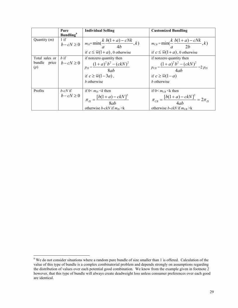
29

Pure Bundling9

Individual Selling Customized Bundling

Quantity (m) 1 if 0b cN− ≥

mIS=

(1 )min( , )4

k b a cNk ka b

+ −

if (1 )c w a≤ + , 0 otherwise

mCB =(1 )min( , )

2k b a cNk ka b

+ −

if (1 )c w a≤ + , 0 otherwise Total sales or bundle price (p)

b if 0b cN− ≥

if nonzero quantity then

pIS =2 2 2(1 ) ( )

8a b ckN

ab+ −

if (1 3 )c w a≥ − , b otherwise

if nonzero quantity then

pCB =2 2 2(1 ) ( )

4a b ckN

ab+ −

=2 pIS

if (1 )c w a≥ − b otherwise

Profits b-cN if 0b cN− ≥

if 0< mIS <k then 2[ (1 ) ]

8ISb a ckN

abπ + −

=

otherwise b-ckN if mIS >k

if 0< mCB <k then 2[ (1 ) ] 2

4CB ISb a ckN

abπ π+ −

= =

otherwise b-ckN if mCB >k

9 We do not consider situations where a random pure bundle of size smaller than 1 is offered. Calculation of the value of this type of bundle is a complex combinatorial problem and depends strongly on assumptions regarding the distribution of values over each potential good combination. We know from the example given in footnote 2 however, that this type of bundle will always create deadweight loss unless consumer preferences over each good are identical.

30

CB: Customized Bundling PB: Pure Bundling IS: Individual Selling

Figure 2a: Profitability of alternative bundling strategies under different marginal costs. Results: CB strictly dominates the other two extreme strategies when c>0. PB is much more sensitive to marginal cost than IS.

Figure 2c: Profitability of alternative bundling varying consumer preferences across goods. Results: CB strictly dominates the other two extreme strategies when a>0. The relative performance of the other two strategies depends on parameter setting. For some parameter settings, IS can be worse than PB.

Figure 2: Profitability comparison of the three approaches

CB

PB

IS

b=1.0k=0.5a=1.0

CB

IS

PB

b=0.9 k=0.6 cN=0.6

Figure 2b: Profitability of alternative bundling varying consumer preferences across goods Results: CB strictly dominates the other two extreme strategies when a>0. The relative performance of the other two strategies depends on parameter setting. For some parameter settings, IS is never worse than PB).

CB

IS

PB

b=0.9 k=0.4 cN=0.6

31

References Adams, W.J. and J.L. Yellen. "Commodity bundling and the burden of monopoly". Quarterly Journal of Economics 90:475-98, 1976.

Armstrong, M. “Multiproduct Nonlinear Pricing.” Econometrica, Vol. 64, No. 1, 1996, pp. 51-75.

Armstrong, M. and J-C Rochet. “Multi-dimensional Screening: A User’s Guide.” European Economics Review, 43, 1999, pp. 959-979.

Bakos, Y. and E. Brynjolfsson. “Aggregation and Disaggregation of Information Goods: Implications for Bundling, Site Licensing and Micropayment Systems”. Available at http://www.gsm.uci.edu/~bakos/aig/aig.html, June 1997.

Bakos, Y. and E. Brynjolfsson. “Bundling Information Goods: Pricing, Profits and Efficiency”. Management Science, Vol. 45. 1999.

Chen, P. Business Model and Pricing Strategies for Digital Products in the Digital Markets. Unpublished Masters Thesis. National Taiwan University, 1997.

Choi, S., Dale O., and A. B. Whinston. The Economics of Electronic Commerce. Macmillan Technical Publishing, Indianapolis, Indiana, 1997.

Chuang, C. I. and Sirbu, M. A. “Optimal Bundling Strategy for Digital Information Goods: Network Delivery of Articles and Subscriptions”. In Information Economics and Policy, 1999.

Fay, S. and J. K. MacKie-Mason. “Competition Between Firms that Bundle Information Goods”, working paper, University of Michigan, July 2001.

Fishburn, P.C., A.M. Odlyzko and R.C. Siders. “Fixed fee versus unit pricing for information goods: competition, equilibria, and price wars”. Proceedings of the Conference on Internet Publishing and Beyond: Economics of Digital Information and Intellectual Property. Cambridge MA. 1997.

Hanson, W. and R.K. Martin. "Optimal bundle pricing". Management Science 36, no. 2: 155-74,1990.

Rochet, J-C, and P. Chone. “Ironing, Sweeping, and Multidimentional Screening.” Econometrica, Vol. 66, No. 4, 1998, pp. 783-826.

Rychlik, T. . “Randomized unbiased nonparametric estimates of nonestimable functionals”, Nonlinear Anal. 30: 4385-4394, 1998.

McFadden, D. “Conditional Logit Analysis of Qualitative Choice Behavior,” in Frontiers in Econometrics, P. Zarembka, eds. Academic Press, NY, 1974.

MacKie-Mason, J.K., J. Riveros and R. S. Gazzale. "Pricing and Bundling Electronic Information Goods: Field Evidence”. 1999.

Metcalfe, B. “It’s all in the scrip—Millicent makes possible subpenny net commerce”. Infoworld. January, 1996.

McAfee, R.P., J. McMillan. "Multidimentsional Incentive Compatibility and Mechanism Design”. Journal of Economic Theory 46: 335-354, 1988.

McAfee, R.P., J. McMillan, and M.D. Whinston. "Multiproduct Monopoly, Commodity Bundling, and Correlation of Values". Quarterly Journal of Economics 104: 371-83, 1989.

Myerson, R. B. “Incentive Compatibility and the Bargaining Problem.” Econometrica, Vol. 47, No. 1., 1979, pp. 61-74.

Owen, D. B. and G. P. Steck. “Moments of Order Statistics from the Equicorrelated Multivariate Normal Distribution”. Annals of Mathematical Statistics, 33(4): 1286-1291, Dec. 1962.

Salinger, M. A. " A Graphical Analysis of Bundling". Journal of Business, 68 (1): 85-98, 1995.

Schmalensee, R. L. “Gaussian demand and commodity bundling”. Journal of Business 57: S211-230,1984.

Shapiro, C. and Varian, H. R.. Information Rules. Cambridge, HBS Press, 1998. Sibley, David S. and Padmanabhan Srinagesh. “Multiproduct nonlinear pricing with multiple taste characteristics”. Rand Journal of Economics. 28 (4). Winter 1997. 684-707.

32

Spence, Michael. “Multi-Product Quantity-Dependent Prices and Profitability Constraints”. Review of Economic Studies, 821-841, 1980.

Stigler, G.J. “United States v. Loew’s Inc.: A Note on Block Booking.” Supreme Court Review, pp. 152-157.

Tirole, J. The Theory of Industrial Organization. MIT Press. Cambridge, MA,1988.

Topkis, D. M. “Minimizing a Submodular Function on a Lattice”, Operations Research, 26 (2): 305-321, 1978.