Bulletin of the Seismological Society of America, Vol. 69, No. 2, pp. 353-368, April 1979

A LOCAL EARTHQUAKE CODA MAGNITUDE AND ITS RELATION TO DURATION, MOMENT Mo, AND LOCAL RICHTER MAGNITUDE ML

BY ANNE M. SUTEAU AND JAMES H. WHITCOMB

ABSTRACT

A relationship is found between the seismic moment, Mo, of shallow local earthquakes, coda amplitudes, and the total duration of the signal, t, in seconds, measured from the earthquake origin time. Following Aki, we assume that the end of the coda is composed of backscattering surface waves due to lateral heterogeneity in the shallow crust. Using the linear relationship between the logarithm of Mo and the local Richter magnitude ML, we obtain a relationship between ML and t, of the form: ML = ao + a 1 log t + a2t 1/~ + f(t), where ao, al , a2 are constants depending on an attenuation parameter (effective Q) and geomet- ric spreading; and f(t) is a function of the instrument response and a (weak) function of the scattering process. This relationship is different from the empir- ical one generally used ML = ao + al log ~- + a2(Iog ~.)2 + a3~, where ~- is the duration measured from the first P arrival time and A is epicentral distance in kilometers. In the theoretical relationship, the dependence on epicentral dis- tance is implicit in t. The theoretical relationship is used to calculate a coda magnitude Mc that is compared to ML for southern California earthquakes which occurred during the period from 1972 to 1975. This comparison is made independently at six stations of the CIT network. At all stations, a good linear fit (ML = Co + C~Mc) is obtained. The standard errors range from 0.2 to 0.3 and the correlation coefficients from 0.80 to 0.90. Once station gain is accounted for, station correction terms are less than 0.17 magnitude unit when comparing ML and Mc. Mc calculation is not limited to a duration measurement but can utilize the entire earthquake coda in order to increase by many times the statistical confidence in an estimate of an earthquake's magnitude.

INTRODUCTION

With the advent of computerized local earthquake analysis systems using large seismographic networks, new methods of earthquake magnitude determinations are needed. Current methods of magnitude determination for local earthquakes, esti- mations that require the amplitude of body waves or the duration of the coda, are not generally useful for computerized systems. In larger earthquakes, body-wave amplitudes can exceed the linear range of the recording system and, in some automated systems, recording can cease before the end of the coda. The intent of this paper is to develop a method of magnitude estimation that can utilize any part of the coda, some of which will certainly be preserved in the linear range of computer recording systems. It is shown how this coda magnitude method relates to other estimates of earthquake size by the use of coda duration, moment Mo, and local Richter magnitude ML.

An empirical correlation between the magnitude of earthquakes, M, and the duration of the recorded signal, T, has been consistently observed. Linear relation- ships between M, log T (~ in seconds), the epicentral distance, A (in kilometers), and the focal depth, h (in kilometers), have been empirically determined for various geographical areas, using multiple regression analysis techniques.

The first study was made by Bisztricsany (1958), who found a linear relationship between the magnitude of teleseisms (in the range of 5 to 8), the logarithm of the

353

3 5 4 A N N E M. S U T E A U A N D J A M E S H. W H I T C O M B

duration of the surface-wave train, and the epicentral distance. Later, this method was applied to local earthquakes (of epicentral distances less than 100 km), with shallow focus (focal depth less than 60 km), and the duration • was defined as the total length of the record, instead of the length of the surface-wave train only. In chronological order, such studies have been due to Solov'ev (1965) for Sakhalin Island; Tsumura (1967) for Japanese earthquakes recorded at the network of the Wakayama Microearthquake Observatory, and whose magnitudes were determined by the Japan Meterological Agency; Crosson (1972) for earthquakes in the Puget Sound Region, using magnitudes calculated from Wood-Anderson records; Lee et al. (1972) for central California earthquakes with Richter magnitude ML; Real and Teng (1973) for southern California also with ML; Herrmann (1975) for the central United States and body-wave magnitude determinations; Bakun and Lindh (1977) for the Oroville, California, region, and ML. Similar studies have been made for the Mica Array, Canada, the Santiago station in Chile, the Alaska network and the University of Utah seismograph stations, U.S.A., etc. (see Lee and Wetmiller, 1976).

For shallow earthquakes, focal depths are much smaller than epicentral distances and much less accurately determined. As a result, it is harder to investigate the dependence of duration on focal depth than on epicentral distance. No such dependence has ever been found in a conclusive way.

The local magnitude ML, introduced by Richter (1935), is given by: ML = log A - log A0 (A, km) where A is the maximum amplitude in millimeters on the Wood- Anderson seismogram for an earthquake at distance A km, and A0 is that for a particular earthquake selected as standard. (All logarithms used here are common logarithms to the base 10.) The magnitudes determined by this method are usually above 2.5, so that, for smaller earthquakes, an equivalent magnitude has to be used. It is obtained by reading the maximum amplitude recorded by a short-period high- gain seismometer and conversion into the amplitude that would have been recorded if a Wood-Anderson instrument had been used.

When plotting the local magnitude ML versus the logarithm of duration, a slight curvature is consistently observed (Lee et al., 1972, Figure 4; Real and Teng, 1973, Figures 5 and 6; Lee and Wetmiller, 1976, page 23; Bakun and Lindh, 1977, Figure 6b). An example for the station MWC is shown in Figure 1 from Real and Teng (1973). The slope increases with increasing magnitude. Consequently, a better fit of the data is obtained by introducing a quadratic term in log T in the magnitude- duration relation. Therefore, the general form of the empirical relation between magnitude and duration is given by

M = ao + al log T + a2(log T) 2 + a3A, (1)

where ao, al, a2, and a3 are constants. Reviews of existing formulas have been given by Real and Teng (1973) and Bakun and Lindh (1977). The standard deviations are in the range of 0.1 to 0.2, the estimated standard errors, of 0.2 ~ 0.3. The dependence on epicentral distance is small and always negligible for distances less than 200 km (e.g., Tsumura, 1967; Crosson, 1972).

As established by Tsumura (1967), the errors in the duration magnitude due to subjective errors in reading durations do not exceed ___0.3 magnitude unit. The main source of observational error is the uncertainty in determining the end of the earthquake signal. Acccording to Real and Teng (1973), it is fixed with an uncertainty of about 20 per cent. It results in an approximately constant uncertainty of log T

C O D A M A G N I T U D E R E L A T E D T O D U R A T I O N , Mo, A N D ML 355

over the range of magni tude of interest, 0.15 unit of magnitude. In the same study, it has been established tha t there is no azimuthal dependence, as long as a sufficient number of events covering a large area and recorded on a long period of t ime (say, a few years) is analyzed, and tha t the effect of variations in microseismic noise is insignificant in southern California.

Theoretical relationship between ML and duration. In this paper, we t ry to find a theoret ical justification for the empirical relationships existing between local magnitude, durat ion of the signal, and epicentral distance. Aki (1969) has proposed a theory in which the coda of local ear thquakes is composed of backscat tered waves due to lateral he terogenei ty in the crust. He has observed tha t the power spectra of coda waves at a given t ime measured from the ear thquake origin t ime ("lapse t ime") appear to be near ly independent of the epicentral distance and of the nature of direct wave pa th between stat ion and epicenter, as can be seen by comparing the records of the same event at different stations (Aki, 1969; Aki and Chouet, 1975). Aki (1969) has constructed his model for coda waves on the following three

4

ML

5

I I I I

MWC

The '

.J.'" .~" (Real and Teng, 197'3)

I l I I I 2 5

log r

FIG. 1. Local Richter magnitude Mr versus log ? (duration) for station MWC. Dashed line is empirical fit of Real and Teng (1973) to their data. Continuous line is the calculation of Me using parameters described in the text. A small vertical offset is introduced to separate the curves.

assumptions: (1) The distribution of the scatterers is two-dimensional over the Ear th ' s surface, r andom and uniform. (2) Th e pr imary waves and the secondary waves are surface waves of the same kind, and a constant group velocity independent of f requency is assumed for them, for the sake of simplicity. (3) Th e distance between stat ion and scat terer is on the same order as the distance between hypocen te r and scat terer and is much larger than the hypocentra l distance. He makes use of the Born approximation by neglecting multiple scattering. He obtains the following relation

Mo[2N(ro)]~/2IOo(fp] ro)] = ~/2 d%t/Q) 1 dt A(t) I(fp )-~ Q (2)

where Mo is the seismic moment , N (ro) is the number of scatterers within a radius of r0, I Go ( fp I ro) I is the absolute value of the Fourier Transform of displacement due

356 A N N E M. SUTEAU AND J A M E S H. WHITCOMB

to secondary waves generated at a scatterer at a distance r0 by a source of unit moment located at the same distance from the scatterer, A( t ) is the average peak- to-peak amplitude on a seismogram estimated from a short time sample around a given absolute lapse time t, I(fp) is the instrument response, and Q is an apparent quality factor, which is assumed constant and includes the effects of intrinsic attenuation of the wave medium and scattering process. The peak frequency f~ was obtained by measuring the wave period directly on the seismogram at time t. For his data (aftershocks of the Parkfield earthquake, June 28, 1966), Aki found the following empirical formula for the peak frequency fp versus the corresponding lapse time t

• f p - - - - I . 5 t

100 (3)

where t is in seconds and f~ is in Hz, in the range 30 ~ t _-< 1000. This relation seems to be independent of earthquake size, epicentral distance, and nature of the direct path between station and epicenter. In the following, we will assume that the same dispersion relation applies to earthquakes studied here. Let B (fp) - [2N (r0) ] :/21 ~o ( fp I r0 ) I. The values of B ( fp ) as a function of peak of frequency have been empirically determined by Aki and are given in his Table 3 (Aki, 1969). Using equation (3), equation (2) becomes

Mo = B ( fp)-I t 11/12 e(~Jv.6~t'/:)/Q) 1_~ Q,/4. A (t)] I ( fp )1 -l (4) 5.24

This formula is strictly valid only in the range of frequencies which are lower than the corner frequency of the particular event under consideration. The effect of the radiation pattern has been neglected, which is a reasonable assumption because the scattered energy should represent a broad range of source azimuths. A linear relationship between the logarithm of seismic moment M,, and the local magnitude ML for a given geographical area has been consistently established in California over a wide range of magnitudes (0 < ML < 6) {e.g., Wyss and Brune, 1968; Aki, 1969; Thatcher and Hanks, 1973; Johnson and McEvilly, 1974; Bakun and Lindh, 1977). No systematic dependence of this Mo-ML relationship on either epicenter location or focal depth has ever been found. Uncertainties in the determination of magnitudes and variation in the geology at the recording site introduce an uncertainty factor of 2 or 3 in relating moment to magnitude (Wyss and Brune, 1968; Johnson and McEvilly, 1974). We will express this relationship in the following way

log Mo = a + bML (5)

where a and b are constants. If we designate M c as a coda magnitude estimate of local Richter magnitude ML, equation (4) can then be rewritten as

1 a + bMc = -0.72 + log A (t) + log B ( fp )-1 _ 4 log Q

11 log t + 17.67 log e t'" + log I I( fp )1 --1 (6) +1-2 Q

CODA MAGNITUDE RELATED TO DURATION, Mo, AND ML 357

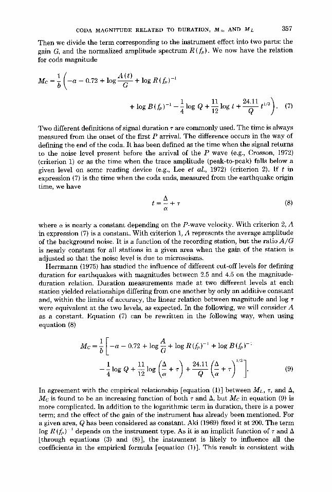
Then we divide the term corresponding to the instrument effect into two parts: the gain G, and the normalized amplitude spectrum R(fp). We now have the relation for coda magnitude

1 ( A( t ) + Mc = -~ - a - 0.72 + lOg-G-- log R(fp) -~

11 24.11 1/3"~ + l o g B ( f p ) - ' - l l ° g q + - ~ l ° g t + - - - ~ - t )" (7)

Two different definitions of signal duration r are commonly used. The time is always measured from the onset of the first P arrival. The difference occurs in the way of defining the end of the coda. It has been defined as the time when the signal returns to the noise level present before the arrival of the P wave (e.g., Crosson, 1972) (criterion 1) or as the time when the trace amplitude (peak-to-peak) falls below a given level on some reading device (e.g., Lee et al., 1972) (criterion 2). If t in expression (7) is the time when the coda ends, measured from the earthquake origin time, we have

h t = - + T (8)

where a is nearly a constant depending on the P-wave velocity. With criterion 2, A in expression (7) is a constant. With criterion 1, A represents the average amplitude of the background noise. It is a function of the recording station, but the ratio A/G is nearly constant for all stations in a given area when the gain of the station is adjusted so that the noise level is due to microseisms.

Herrmann {1975) has studied the influence of different cut-off levels for defining duration for earthquakes with magnitudes between 2.5 and 4.5 on the magnitude- duration relation. Duration measurements made at two different levels at each station yielded relationships differing from one another by only an additive constant and, within the limits of accuracy, the linear relation between magnitude and log r were equivalent at the two levels, as expected. In the following, we will consider A as a constant. Equation (7) can be rewritten in the following way, when using equation (8)

1 - a - 0.72 + l o g ~ + logR(/~) -1 + l o g B ( ~ ) -1 Mc=~

- - l l ° g Q + ] 2 l ° g 4 + ' r +1" . (9)

In agreement with the empirical relationship [equation (1)] between ML, r, and h, Mc is found to be an increasing function of both • and A, but Mc in equation (9) is more complicated. In addition to the logarithmic term in duration, there is a power term; and the effect of the gain of the instrument has already been mentioned. For a given area, Q has been considered as constant. Aki (1969) fixed it at 200. The term log R (fp)-~ depends on the instrument type. As it is an implicit function of • and A [through equations (3) and (8)], the instrument is likely to influence all the coefficients in the empirical formula [equation (1)]. This result is consistent with

358 ANNE M. SUTEAU AND JAMES H. WHITCOMB

the observations of Bakun and Lindh (1977): They plotted ML versus log r for three different instruments and found a different intercept and a different slope in each case (their Figure 6b). The USGS and ORV instruments, which have about the same normalized response below 5 Hz, gave about the same slope, whereas the ORV-LP instrument which has a normalized response very different from the two others gave a different slope (their Figure 2).

DATA ANALYSIS

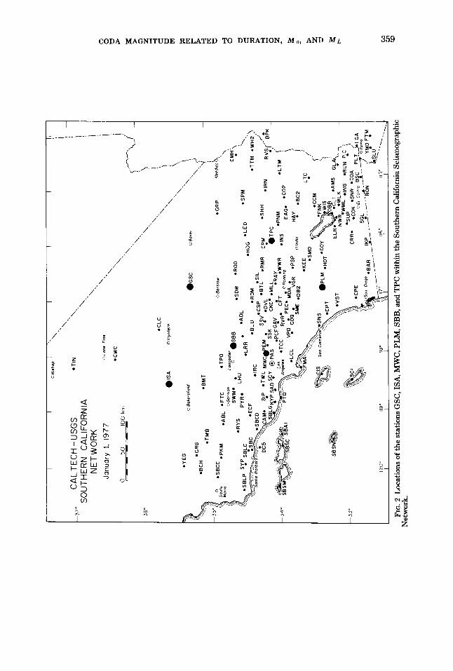
In order to further check the duration-Mr relationship, we now compare local magnitudes ML with Me from the theoretical expression (9) for events in southern California recorded during the period from 1972 to 1975. The following stations of the telemetered seismic network operated by the Seismological Laboratory of the California Institute of Technology have been used: Isabella (ISA), Goldstone (GSC), Saddleback Butte (SBB), Mount Wilson (MWC), Twentynine Palms {TPC), and Palomar (PLM). Their locations in the Southern California Seismograph Network are shown in Figure 2. The signal was recorded by short-period vertical Benioff seismometers and registered on drum recorders revolving at a speed of 60 mm/min. Durations r were read using criterion 2, the average peak-to-peak amplitude thresh- old, A, being approximately 0.1 cm. The gain G was initially assumed to be the one at the station PAS, GeAs, of 10 '~. The effect of different gains is discussed below. The coefficient a of expression (9) was taken as 6.17 km/sec, Q fixed at 200 following Aki {1969) and the values of B(fp) were taken from Aki's Table 3, once fp had been determined from r and h using relations (3) and {8). The constants a and b in the moment-magnitude relation (5) that we used were also determined by Aki {1969) in his study of aftershocks of the Parkfield earthquake; for the magnitude range of 3 to 5.5 he found

log 214o = 15.8 + 1.5 ML. (10)

In this way, we have calculated a coda magnitude Mc for each event at each of the six stations, as expressed by

1 1 Me = -12.07 - ~-~ log GeAs + ~--~ log R (fp)-i

,11,

and shown in Table 1 [for t < 60 sec, values for B(fp) used in Table 1 are different from Aki, as discussed below]. R (fp) is the normalized instrument response of the short-period Benioff seismometer. Figure 3 shows the correlation between ML and Mc. Mr ranged from 2.6 to 5.5. Below 2.6, most values of ML have been obtained from short-period seismograms instead of Wood-Anderson records and they are omitted.

The results of a least-squares fit of the data for each station for ML ~ 2.6 are given in Table 2, including also the geographic coordinates of the stations, the period of time during which the data have been obtained, the number of events used in the analysis, the standard error of estimate, and the correlation coefficient. The standard errors are 0.2 - 0.3 which is comparable to what is usually obtained by fitting such data with an empirical relationship of the form of expression {1). The correlation coefficients range from 0.80 for MWC where there is much scatter in the data,

C O D A M A G N I T U D E R E L A T E D T O D U R A T I O N , Mo, A N D M L 3 5 9

I [

/ ' "

/

/

/ "

/

/ /

/ /

/

o 0 •

°- I

0

k

T

. /

i

/ /

/ /

/ ~: /

/ ~

/ /

o

/

I - / .. ',._. . . . . . ~ % ~ / i

o ~ ~; ~ : . z ~ ' ~ m "

~ ~ . ~ . • ~ ~ . ~.~

~ . o ~ ~ ~ ~ ~;

o_ l ..1 e ~ e~ I-- ..I 0 > b.I c~ ~o

• a. > o ",~ • o e o ~ o~

~ . . . . . . .

~.~ : ~ o-~ "~ ~ ~

• ~ ~ I®.~ ~ :~

.~

i

0

ID

0

I.-

0

o

,,> '-L

360 ANNE M. SUTEAU AND JAMES H. WHITCOMB

p a r t i c u l a r l y a t l o w m a g n i t u d e s , t o 0.90 f o r I S A . T h e n u m b e r o f e v e n t s is o n t h e

o r d e r o f 300 - 400, d e p e n d i n g o n t h e s t a t i o n , a n d t h e d a t a h a v e b e e n o b t a i n e d

b e t w e e n 1973 a n d 1975 f o r m o s t s t a t i o n s , so t h a t t h e a z i m u t h a l c o v e r a g e is g o o d a n d

t h e e v e n t s h a v e a b r o a d d i s t r i b u t i o n in s ize , e p i c e n t r a l d i s t a n c e , a n d s o u r c e m e c h -

a n i s m .

TABLE 1

CALCULATION OF THE CODA M A G N I T U D E Mc

t f,, log R(f~,)-' (see) (Hz)

Mc

Q = 500 200 70

5 6.04 --4.98 1.82 1.71 1.38 7 4.83 --5.00 1.91 1.80 1.51

10 3.81 --4.97 2.03 1.94 1.68 12 3.37 --4.94 2.10 2.02 1.78 15 2.90 --4.90 2.19 2.12 1.90 20 2.40 --4.84 2.32 2.25 2.08 30 1.83 --4.70 2.53 2.49 2.37 40 1.51 --4.58 2.70 2.67 2.59 50 1.30 --4.48 2.83 2.82 2.78 60 1.15 --4.38 2.95 2.95 2.95 70 1.04 --4.31 3.05 3.05 3.08 80 0.95 --4.24 3.14 3.15 3.21 90 0.88 --4.16 3.23 3.25 3.33

100 0.82 --4.08 3.31 3.34 3.45 120 0.73 --3.99 3.43 3.47 3.63 150 0.63 --3.82 3.62 3.68 3.89 200 0.52 --3.59 3.86 3.95 4.24 300 0.39 --3.28 4.20 4.33 4.75 400 0.33 --3.04 4.46 4.62 5.14 500 0.28 --2.89 4.64 4.83 5.43 600 0.25 --2.73 4.81 5.02 5.70 700 0.22 --2.60 4.95 5.19 5.93

TABLE 2

FIT OF M c = bo + b, ML

Number of Correlation Std. Error of

Station Latitude Longitude Period Events With ML b~) bl Coefficient Estimate

> 2.6

GSC 35°18.1'N 116°48.3'W 1973-1975 308 1.11 0.75 +_ 0.03 0.86 0.23 ISA 35039.8 , 118o28.4 , 1973-1975 288 1.27 0.73 +_ 0.02 0.90 0.18 MWC 34013.4 ' 118003.5 , 1972-1975 346 1.14 0.72 _ 0.03 0.80 0.26 PLM 33021.2 , 116°51.7 ' 1973-1975 402 1.58 0.64 +_ 0.02 0.81 0.22 SBB 34041.3 ' 117049.5 , 1974-1975 292 1.44 0.69 _ 0.03 0.85 0.21 TPC 34006.4 , 116o02.9 , 1973-1975 298 0.96 0.82 _ 0.03 0.83 0.27

DISCUSSION

The relationship between Me and ML is put in a more convenient form when it is written as

M L = Co + C i M c (12)

a n d t h e s e p a r a m e t e r s a r e s h o w n in T a b l e 3. I t c a n b e s e e n t h a t t h e s l o p e C1 is

s y s t e m a t i c a l l y t o o h i g h , t a k i n g v a l u e s b e t w e e n 1.22 a n d 1.55, t h e a v e r a g e v a l u e b e i n g

1.4. W e n o w e v a l u a t e w h a t p a r a m e t e r s o f t h e t h e o r y c a n a f f e c t t h e s l o p e a n d a r e

t h e r e f o r e c o r r e l a t e d .

CODA M A G N I T U D E R E L A T E D TO D U R A T I O N , JYIo, A N D ML 361

Aki and Chouet (1975) have also proposed a second model for coda waves in which the seismic energy transfer was considered as a diffusion process. With the diffusion theory, the geometrical spreading term t 1/2 in equation (2) is replaced by t 3/4, i.e., a power intermediate to 1 (corresponding to body waves) and ½ (surface waves). It is easily seen that this would change only the coefficient of log(h/a + ~) in the theoretical expression giving the coda magnitude (9), and (11), from 0.61 to

M L 4

e 4 i i i i • / /

GSC / • /

e / • e / •

o • • o ~ /

• • e •

~ g ' o o

•

.: .::.~. -.

~1 I I I I

n I I I I

MWC . , / •

• / / / •

• o • m m m e o

• , o • • o

• e 4 m ~ u ~ e o •

/

¢ I I F I I

i i i I ~

SBB ,' • /

/ •

/

i ' I

i i r I r r

ISA ,," / •

• / , N

o , ' e

• _'o,, .., e e

i i nl

i nl •

/ r I r 4 I i

n i J i I u e /

PLM / • / /

/ • /

/ • • /

/ . i

• e ° ° ~ e : . -

• .

i J l J J i

/

I / I I i I

J i ~ I n

TPC ,-" , i

,,,; e"

/ , * . • . e~o

ae~ eoe*

. . : . ' - . : - .--.

• ,.';'.-%" -. • o ~

• 'o,,. 'r"?~.. • e ~ a •

/

4 5 M c

FIG. 3. Correlation between ML and Mc for the stations GSC, ISA, MWC, PLM, SBB, and TPC. The parameters for the linear least square fits are given in Table 2.

0.78. The diffusion theory applies only to the parts of the energy scattered in the backward direction. Like the single-scattering theory that we have used, it is a simplification, and probably, the actual power of the geometrical spreading term lies

:3 (diffusion process), between the values of ½ (single-scattered surface waves) and and the calculated slopes are shown in Figure 4. For the frequencies used here, Aki

362 A N N E M. S U T E A U A N D J A M E S H. W H I T C O M B

and Chouet conclude that the coda is mostly back-scattered surface waves. The effect of incorporating a diffusion process theory would reduce the observed slopes from 1.4 to about 1.3, which is not a significant difference. The coda magnitude M c for each event recorded at each station has been calculated from expression (11). This expression makes use of the empirical dispersion law [equation (3)] for coda waves found by Aki for the Parkfield region (Aki, 1969). A pr ior i , this law does not apply to our set of data and a more rigorous t rea tment would necessitate a derivation of a similar law for the data used in this study. Any discrepancy between the actual

TABLE 3 FIT OF ML = Co + C~ Mc AND GAIN CORRECTION

~G ~ML Residual

(~..15 GST̂ ) (eale.-obs.) AML-hG Station Co C~ Gain GSTA log ~ at Mr, = 3.1

GSC -1.48 1.34 4.80 × 105 0.46 0.34 -0.12 ISA -1.73 1.37 2.40 0.26 0.43 +0.17 MWC -1.58 1.38 2.37 0.25 0.27 +0.02 PLM -2.45 1.55 4.83 0.46 0.46 +0.00 SBB -2.10 1.46 8.00 0.61 0.48 -0.13 TPC -1.17 1.22 3.76 0.39 0.40 +0.01

/ / /

51-- / / / (a) Backscattering

~-/ / (c) Backscattering V / body woves

21/" t I ~ I 2 5 Mc 4 5

FIG 4 The change in slope of Mc due to different geometrical spreading terms (following Aki and Chouet, 1977) for (a) t 1, backscattering body waves, (b) t w~, diffusion process, and (c) t in, backscattering surface waves.

dispersion law and the one we used may yield a slope different from 1 in the M L versus M c curve and even to a curvature of this line. In order to get M c , we also used the values of B ( f p ) tabulated by Aki (1969). These values were obtained by fitting the data in his Figure 3. There are not many data for peak frequencies between 0.2 and 1 Hz, which is the range of frequency corresponding to the durations of most events with magnitudes between 2.6 and 5.5. Therefore, the function B (fp) is not well constrained and may be subject to reevaluation; adjus tment of any of the slope-changing parameters will affect B (fp). However, the two most likely candidates

CODA MAGNITUDE RELATED TO DURATION, Mo, AND M L 363

to change the slope of the ML versus M c correlations are either the Mo versus ML relationship or Q.

Mo-ML relationship. Wyss and Brune (1968) have Fourier analyzed surface waves from 13 earthquakes in the Parkfield region and have found the following relation- ship between seismic moment Mo and Richter magnitude ML

log Mo = 1.4 ML + 17.0,

for 3.2 < ML < 5.5. Mo of southern California earthquakes calculated by Thatcher and Hanks (1973) from long-period S-wave spectral levels yielded the relation

log Mo = 1.5 ML + 16.0,

for ML between 2.5 and 6. These two studies give a coefficient b of 1.4 - 1.5, similar to the one found by Aki (equation 10). However, more recent studies in central California have yielded a coefficient b closer to 1. Johnson and McEvilly (1974) have estimated seismic moments from the low-frequency levels of the spectra for 13 earthquakes with magnitudes between 2.4 and 5.1 located near the San Andreas fault and found the following relation

log 3/lo = (1.16 + 0.06)ML + (17.60 _ 0.28).

And for earthquakes near Oroville, Bakun and Lindh (1976) have found

log Mo = (1.21 __ 0.03)ML + (17.02 _ 0.07)

for 0 < ML < 6. The value of 1.5 for the coefficient of ML in the moment-magnitude relation may be more appropriate for southern California than the value of 1.2 found for central California. However, a coefficient b closer to 1 would explain the average slope C1 higher than 1 found for our ML versus Mc curves. In fact, if the actual value of b was 1.2 instead of 1.5, this slope would be reduced from 1.4 to 1.1.

Effective Q. In our calculation of coda magnitude Mc, we have used a Q of 200 (Aki, 1969). However, a lower value may be more realistic, since values of 50 to 200 at frequencies on the order of 1 Hz have been found for the Q of coda waves in central California and western Japan (Aki and Chouet, 1975). At these frequencies (0.2 to 2 Hz) which are dominant at the end of the coda of local earthquakes, the coda is probably made of backscattering surface waves from heterogeneities in the shallow, low Q crust. If the actual average apparent Q of coda waves of local earthquakes in southern California was 70, a value favored by Aki and Chouet (1975), instead of 200, the observed scope C1 of ML versus Mc relationship (12) would be reduced from 1.4 to about 1.1 as seen in Figure 5.

In order to investigate the influence of gain of the instrument and/or geology at the station site on the coda magnitude Mc, we now consider the difference ~//L between the calculated ML from equation (12) and the observed ML for a well- sampled interval of magnitude, chosen around Mc = 3.1. If M c is a good approxi- mation of ML there should be a station gain correction for each station relating the assumed station gain of Gens (10 "~) to the actual station gain GSTA from equation (11) as follows

1 GSTA AG = 1-~ log Gpns" (13)

364 ANNE M. SUTEAU AND JAMES H. WHITCOMB

Table 3 shows the values of the stat ion gains, AG, ~/IL, and the residual of ~ / / L - -

AG. I t is clear f rom this table tha t the major contr ibution to the discrepancy between calculated and observed ML is due to the effect of the gain at each part icular station. A coda excitation factor, depending on the surface geology of the station site, should have the same effect on the magnitude residuals as the gain of the instrument. This factor can be 5 to 8 t imes larger on sediments than on granite (Aki, 1969), which corresponds to a relat ive change of 0.5 to 0.6 in magnitude. ML is overest imated at ISA by 0.17 and underes t imated at SBB by 0.13, with the other stations intermediate to these values. These corrections may be insignificant considering the scat ter of the data. All of the stations used in this s tudy are sited directly on crystalline bedrock (granite or metamorphic) , with the exception of Palomar, which has a few meters of alluvium between the ins t rument and the granitic bedrock. All are essentially on the ground surface except for Isabella, which is about 70 meters in a

4 - -

2v ~ I 2 5

y /

I

M c

I 4

FIG. 5. The change in slope of Mc due to different values of Q. A value close to 70 fits the data of Figures 3 and 6. A Q of 500 fits the data of Figure 1.

tunnel in bedrock. Note tha t the excitation factor should more generally be a function of frequency, so tha t it could not only shift the ML versus Mc curve but also distort it.

We now compare the theoretical magnitude Mc from equation (9) with the empirical curve of our Figure 1 found by Real and Teng (1973) for durat ions at s tat ion MWC: M~ = 1.37 + 0.41 (log v)2 (the distance te rm is neglected). If we assume the same parameters as used above in calculation of Mc, except for an allowance of variance of Q for a good fit, we get the theoret ical curve shown in Figure 1, which is calculated with a Q of 500. (Because prel iminary results have shown no significant variat ion in the scattering proper ty te rm B (f~), it is assigned a constant value of 4.32 x 10 -2'~ which is of course dependent on Q. This has only minor effects on the shape of the low-magnitude end of the curve.) In the empirical relat ionship of Real and Teng, the curvature comes from a (log ~.)2 te rm whereas in

C O D A M A G N I T U D E R E L A T E D T O D U R A T I O N , Mo, A N D ML 365

the M c curve it comes f rom a T '/3 term. I t is interest ing to note t ha t expansion of r a in a series is

2.3a 1 (2"3a)2 r ~ = 1 + ~ o g r + ~ ( l o g ' r ) 2 + . . . .

Thus , the next t e r m after log T is a (log r)2 t e rm in paral lel with Real and Teng ' s empirical fit. The re is, however, a d iscrepancy be tween the durat ion da ta of Real and Teng and tha t analyzed here. I t is represen ted by the fact tha t the fo rmer is be t te r fit with a high Q of abou t 500 whereas our da ta requires a lower Q of abou t 70. At the presen t this difference is not understood. The da ta of Real and Teng were ga thered f rom 1969 to 1971 events and the da ta here are f rom 1972 th rough 1975. This presents the possibil i ty of a change of Q be tween the intervals. Alternat ively, a l though the reading me thods were supposedly the same, it is possible t ha t var iances

6 I I f l

- - . / , 7

4 ~P

M L

0 Q - -

2 / / - / , / vOb~r_ved Theoreticol OR

~ ORV-LP '-' I I

I 2 5 Log -r

FIG. 6. Local Richter magnitude ML v e r s u s log r (duration) for stations ORV and ORV-LP. Dashed line and squares are linear fits to data and data for ORV and ORV-LP, respectively, from Bakun and Lindh (1977). Solid lines are the theoretical coda magnitude Mc calculated with Q = 70 for ORV and ORV-LP to illustrate the effect of different instrument response. Mc for ORV-LP is not defined below ML = 4.4 for this particular value of Q.

in definit ion of the "end" of the coda for large and small events can occur be tween readers. Whe the r these or o ther causes are responsible is a subject tha t deserves fur ther study.

Because the M c magni tude is a funct ion of ins t rument response, it is interest ing to compare the theoret ical M c with durat ion da ta of Bakun and Lindh (1977). T h e y found a different durat ion magni tude relat ion for the ins t ruments ORV, a Benioff se ismometer , and ORV-LP, a long-period ins t rument with peak gain a t abou t 0.2 Hz. Figure 6 shows Mc calculated with a Q of 70 compared with the empirical piece- wise l inear fits of Bakun and Lindh to ORV and ORV-LP data. (A cons tant value of B (f~) = 6.24 × 10 -23 was used for the M e calculation.) T h e Benioff ORV data are fit well except at the b reak in the two l inear empirical curves. Bu t more important ly , the ORV-LP data show marked ly shor ter durat ions t han ORV below ML = 5.5 in ag reemen t with the theoret ical curves. The theoret ical M c curve is not defined below abou t ML ---- 4.4. This implies that , because of the drop-off of ORV-LP

366 A N N E M. S U T E A U A N D J A M E S H . W H I T C O M B

instrument response with higher frequency above 6 Hz combined with smaller earthquake amplitudes, scattered energy drops below the noise level of the seismo- gram.

A consideration that compromises the extension of duration and coda magnitude scales to small earthquakes is the evidence that the later part of the coda is mainly composed of backscattered waves. Certainly this is not true at the time of the direct S-wave arrival. Depending on the length of what one considers "S-wave" on the seismogram, it is reasonable to suppose that within 5 to 10 seconds of the S-wave arrival we are dealing more with the direct S-wave energy. Comparison of times of this order with those in Table 1 imply that extrapolations of duration and coda magnitude scales below about ML = 1.5 should be carefully reevaluated.

In Table 1 are summarized the Mc values calculated for the coda at t, the time from origin time, for 0.1 cm RMS amphtude at a station with 1 × 10 ~ gain. Mc values for Q's of 500, used in Figure 1, 200, used in Figure 3, and 70, used in Figure 6, are given to illustrate the effect of variable Q. In these tables, the scattering property B (fp) is assumed constant and adjusted such that Mc values at t = 60 sec are equal. Again, the assumption that B (fp) is constant instead of variable as in Aki (1969) significantly affects only magnitudes below ML = 2.6 and would result in a reduction of the lower values by about 0.3 magnitude units if the Aki values were used. Study of this parameter will be done in a future paper. An important point to note here is that Q can be an important factor in relating the coda magnitudes of small earthquakes to large earthquakes. The difference in coda magnitude can be as large as one unit over a n ML range of 3 to 5 for published data in the literature. This result makes the calibration of individual stations for Q an important consideration in the establishment of a coda magnitude scale.

The use of Mc values in Table 1 for any part of the coda involves only an additive term for the coda amplitude at the corresponding time as can be seen in equation (7). Different instrument gain requires an added constant in the same equation. Use of a different instrument response requires the removal of the Benioff response term in Table 1 or equation (7), log R(f~) ~, and addition of the equivalent term corresponding to the desired instrument response.

CONCLUSIONS

Backscattering surface waves due to lateral heterogeneity in the shallow crust appear to be a good explanation for the late part of the coda of local earthquakes and duration times. The scattering theory measures the moment Mo and provides a physical basis for the observed empirical correlation between local Richter magnitude ML and total duration of the coda.

With the use of the scattering theory, we derive a coda magnitude Mc that can be used at any part of the coda and, in particular, where durations are measured. We compare ML to the coda magnitude Mc calculated from duration data at six stations of the CIT network. For a linear fitML = Co + CIMc, we find slopes CI systematically higher than one with the use of our initial assumptions based on the parameters of Aki (1969). This high value of Ca implies one, or more likely a combination, of the following factors: the coda waves may have a geometrical spreading factor inter- mediate between surface waves and body waves; the coefficient b of 1.5 in the ML- Mo relationship may be too high; the apparent Q of 200 that is used is too high and a value of 70 may be more appropriate.

For the six bedrock stations analyzed here, a correction for station gain within the theoretical framework of Mc removes all significant site correction factors from the

CODA MAGNITUDE RELATED TO DURATION, !glo, AND M L 367

duration data. The remaining site correction on "coda excitation" terms deviate less than 0.17 magnitude units from the average.

Comparison of the coda magnitude Mc with the duration data of Real and Teng (1973) shows that the theoretical Mc matches the curvature of the data that led Real and Teng to add a higher order term to their fit of ML versus log r. However, a high Q of 500 in the Me relation was necessary to fit their data. Comparison of Mc with the duration data on Bakun and Lindh (1977) shows the effect of different instrument response on the duration data. With a Q of 70, the Mc calculation fits their short-period Benioff data from ORV and simultaneously fits the widely divergent long-period ORV-LP data for magnitudes above ML = 4.4.

The results here strongly support the theory that the coda is composed of scattered energy. However, that same theory implies that scattering assumptions do not hold in the early part of the S-wave coda. For this reason, it appears that the extrapolation of duration and coda magnitude scales below ML = 1.5 should be carefully reevaluated.

The coda magnitude Mc can be used either with coda duration data or with any portion of the coda that is not "close" to the direct S-wave arrival. The latter feature is important for the usefulness of Mc in computerized seismic data systems where parts of the coda may exceed the system's linear range, preventing the calculation of a body-wave magnitude, or may be cut off before the time where duration would normally be measured. Use of the entire coda of each recording seismic station should provide a more robust estimate of magnitude.

Most importantly, the coda magnitude Mc has a physical basis that relates moment Mo, Richter magnitude ML, duration and the general shape of the coda to the station gain, instrument response, and effective Q. There is evidence here that effective Q can vary significantly from station to station which may require a calibration of individual stations. The study of regional variation of effective Q and other parameters that affect the theory of scattered coda energy will be the subject of future investigations.

ACKNOWLEDGMENTS

The authors wish to thank Don Anderson, Keiiti Aki, William Bakun, Carl Johnson, Karen McNally, and Bernard Minster for critically reviewing the manuscript and providing several helpful suggestions. The data used in this paper is due to many individuals at the Seismological Laboratory who maintain the network and process the data and their efforts are greatly appreciated. This work was supported by JPL/ NASA Contract 49-681-02081-0-3260, NASA Grant NSG-5224, and U.S.G.S. Contract 14-08-0001-16719.

REFERENCES Aki, K. (1969). Analysis of the seismic coda of local earthquakes as scattered waves, J. Geophys. Res. 74,

615-631. Aki, K. and B. Chouet (1975). Origin of coda waves: Source, attenuation, and scattering effects, J.

Geophys. Res. 80, 3322-3342. Bakun, W. H. and A. G. Lindh (1977). Local magnitudes, seismic moments and coda durations for

earthquakes near Oroville, California, Bull. Seism. Soc. Am. 67, 615-629. Bisztricsany, E. (1958). A new method for the determination of the magnitude of earthquakes, Geofiz,

Kozlemen. 7, 69-96. Crosson, R. S. (1972). Small earthquakes, structure, and tectonics of the Puget Sound region, Bull. Seism.

Soc. Am. 62, 1133-1177. Herrmann, R. B. (1975). The use of duration as a measure of seismic moment and magnitude, Bull.

Seism. Soc. Am. 65, 899-913. Johnson, L. R. and T. V. McEvilly {1974). Near-field observations and source parameters of Central

California earthquakes. Bull. Seism. Soc. Am. 64, 1855-1886.

368 ANNE M. SUTEAU AND JAMES H. WHITCOMB

Lee, W. H. K., R. E. Bennet, and K. L. Meahger (1972). A method of estimating magnitude of local earthquakes from signal duration, U.S. Geol. Surv., Open File Rept. 28 pp.

Lee, W. H. K. and R. J. Wetmiller (1976). A survey of practice in determining magnitude of near earthquakes: Summary report for networks in North, Central and South America, U.S. Geol. Surv., Open File Rept. 76-677.

Real, C. R. and T. L. Teng {1973). Local Richter magnitude and total signal duration in southern California, Bull. Seism. Soc. Am. 63, 1809-1827.

Richter, C. F. (1935}. An instrumental earthquake magnitude scale, Bull. Seism. Soc. Am. 25, 1-32. Solov'ev, S. L. (1965). Seismicity of Sakhalin, Bull. Earthquake Res. Inst., Tokyo Univ. 43, 95-102. Thatcher, W. and T. C. Hanks (1973}. Source parameters of southern California earthquakes, J. Geophys.

Res. 78, 8547-8576. Tsumura, K. (1967). Determination of earthquake magnitude from total duration of oscillation, Bull.

Earthquake Res. Inst., Tokyo Univ. 15, 7-18. Wyss, M. and Y. N. Brune (1968) Seismic moment, stress, and source dimensions for earthquakes in the

California-Nevada region, J. Geophys. Res. 73, 4681-4694.

SEISMOLOGICAL LABORATORY DIVISION OF GEOLOGICAL AND PLANETARY SCIENCES CALIFORNIA INSTITUTE OF TECHNOLOGY PASADENA, CALIFORNIA 91125 CONTRIBUTION NO. 3062

Manuscript received July 28, 1978