Building Reliable Test and Training Collections in ... · Building Reliable Test and Training...
150
Building Reliable Test and Training Collections in Information Retrieval A dissertation presented by Evangelos Kanoulas to the Faculty of the Graduate School of the College of Computer and Information Science in partial fulfillment of the requirements for the degree of Doctor of Philosophy Northeastern University Boston, Massachusetts December, 2009
Transcript of Building Reliable Test and Training Collections in ... · Building Reliable Test and Training...

Building Reliable Test and Training Collections in Information Retrieval
A dissertation presented
by
Evangelos Kanoulas
to the Faculty of the Graduate School
of the College of Computer and Information Science
in partial fulfillment of the requirements for the degree of
Doctor of Philosophy
Northeastern University
Boston, Massachusetts
December, 2009

Abstract
Research in Information Retrieval has significantly benefited from the availability of stan-
dard test collections and the use of these collections for comparative evaluation of the ef-
fectiveness of different retrieval system configurations in controlled laboratory experiments.
In an attempt to design large and reliable test collections decisions regarding the assembly
of the document corpus, the selection of topics, the formation of relevance judgments and
the development of evaluation measures are particularly critical and affect both the cost of
the constructed test collections and the effectiveness in evaluating retrieval systems. Fur-
thermore, recently, building retrieval systems has been viewed as a machine learning task
resulting in the development of a learning-to-rank methodology widely adopted by the com-
munity. It is apparent that the design and construction methodology of learning collections,
along with the selection of the evaluation measure to be optimized significantly affects the
quality of the resulting retrieval system. In this work we consider the construction of re-
liable and efficient test and training collections to be used in the evaluation of retrieval
systems and in the development of new and effective ranking functions. In the process of
building such collections we investigate methods of selecting the appropriate documents
and queries to be judged and we proposed evaluation metrics that can better capture the
overall effectiveness of the retrieval systems under study.
i


Contents
Abstract i
Contents iii
List of Figures vii
List of Tables xi
1 Introduction 1
1.1 Evaluation . . . . . . . . . . . . . . . . . . . . . . . . . . . . . . . . . . . . 3
1.2 Learning-to-Rank . . . . . . . . . . . . . . . . . . . . . . . . . . . . . . . . 5
1.3 Evaluation metrics . . . . . . . . . . . . . . . . . . . . . . . . . . . . . . . 5
1.4 Duality between evaluation and learning-to-rank . . . . . . . . . . . . . . 6
1.5 Contributions . . . . . . . . . . . . . . . . . . . . . . . . . . . . . . . . . . 7
2 Background Information 9
2.1 Retrieval Models and Relevance . . . . . . . . . . . . . . . . . . . . . . . . 9
2.2 Evaluation . . . . . . . . . . . . . . . . . . . . . . . . . . . . . . . . . . . . 11
2.2.1 Document corpora . . . . . . . . . . . . . . . . . . . . . . . . . . . 12
2.2.2 Topics . . . . . . . . . . . . . . . . . . . . . . . . . . . . . . . . . . 13
2.2.3 Relevance Judgments . . . . . . . . . . . . . . . . . . . . . . . . . 14
2.2.4 Reliability of Evaluation . . . . . . . . . . . . . . . . . . . . . . . . 17
2.3 Learning-to-Rank . . . . . . . . . . . . . . . . . . . . . . . . . . . . . . . . 19
2.3.1 Learning-to-rank algorithms . . . . . . . . . . . . . . . . . . . . . . 19
2.3.2 Learning-to-rank collections . . . . . . . . . . . . . . . . . . . . . . 19
2.4 Evaluation Metrics . . . . . . . . . . . . . . . . . . . . . . . . . . . . . . . 21
2.4.1 Evaluating evaluation metrics . . . . . . . . . . . . . . . . . . . . . 24
2.4.2 Evaluation metrics for incomplete relevance judgments . . . . . . . 25
2.4.3 Multi-graded evaluation metrics . . . . . . . . . . . . . . . . . . . . 25
2.5 Summary and Directions . . . . . . . . . . . . . . . . . . . . . . . . . . . . 27
iii
iv CONTENTS
3 Test Collections 29
3.1 Document Selection Methodology for Efficient Evaluation . . . . . . . . . 29
3.1.1 Confidence Intervals for infAP . . . . . . . . . . . . . . . . . . . . . 31
3.1.2 Inferred AP on Nonrandom Judgments . . . . . . . . . . . . . . . . 34
3.1.3 Inferred AP in TREC Terabyte . . . . . . . . . . . . . . . . . . . . . 37
3.1.4 Estimation of nDCG with Incomplete Judgments . . . . . . . . . . 40
3.1.5 Overall Results . . . . . . . . . . . . . . . . . . . . . . . . . . . . . 42
3.1.6 Conclusions . . . . . . . . . . . . . . . . . . . . . . . . . . . . . . . 43
3.2 Evaluation over Thousands of Queries . . . . . . . . . . . . . . . . . . . . 45
3.2.1 Methods . . . . . . . . . . . . . . . . . . . . . . . . . . . . . . . . . 46
3.2.2 Million Query 2007 : Experiment and Results . . . . . . . . . . . . 47
3.2.3 Million Query 2007 : Analysis . . . . . . . . . . . . . . . . . . . . . 50
3.2.4 Million Query 2008 : Experiment and Results . . . . . . . . . . . . 51
3.2.5 Million Query 2008 : Analysis . . . . . . . . . . . . . . . . . . . . . 54
3.2.6 Conclusion . . . . . . . . . . . . . . . . . . . . . . . . . . . . . . . 60
3.3 Overall Conclusions . . . . . . . . . . . . . . . . . . . . . . . . . . . . . . 61
4 Training Collections 63
4.1 Methodology . . . . . . . . . . . . . . . . . . . . . . . . . . . . . . . . . . 64
4.1.1 Data sets . . . . . . . . . . . . . . . . . . . . . . . . . . . . . . . . 65
4.1.2 Document selection . . . . . . . . . . . . . . . . . . . . . . . . . . 66
4.1.3 Learning-to-rank algorithms . . . . . . . . . . . . . . . . . . . . . . 69
4.2 Results . . . . . . . . . . . . . . . . . . . . . . . . . . . . . . . . . . . . . . 70
4.3 Overall Conclusions . . . . . . . . . . . . . . . . . . . . . . . . . . . . . . 75
5 Evaluation Metrics 77
5.1 Gain and Discount Function for nDCG . . . . . . . . . . . . . . . . . . . . 79
5.1.1 Methodology . . . . . . . . . . . . . . . . . . . . . . . . . . . . . . 80
5.1.2 Results . . . . . . . . . . . . . . . . . . . . . . . . . . . . . . . . . . 82
5.1.3 Conclusions . . . . . . . . . . . . . . . . . . . . . . . . . . . . . . . 94
5.2 Extension of Average Precision to Graded Relevance Judgments . . . . . . 95
5.2.1 Graded Average Precision (GAP) . . . . . . . . . . . . . . . . . . . 96
5.2.2 Properties of GAP . . . . . . . . . . . . . . . . . . . . . . . . . . . . 98
5.2.3 Evaluation Methodology and Results . . . . . . . . . . . . . . . . . 103
5.2.4 GAP for Learning to Rank . . . . . . . . . . . . . . . . . . . . . . . 108
5.2.5 Conclusions . . . . . . . . . . . . . . . . . . . . . . . . . . . . . . . 110
5.3 Overall Conclusions . . . . . . . . . . . . . . . . . . . . . . . . . . . . . . 110
v
6 Conclusions 113
Bibliography 115
A Confidence Intervals for Inferred Average Precision 131
B Variance Decomposition Analysis 133
C Statistics 135

List of Figures
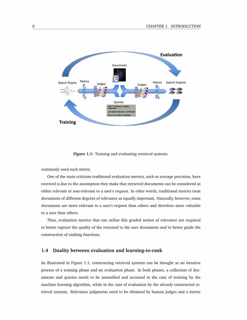
1.1 Training and evaluating retrieval systems. . . . . . . . . . . . . . . . . . . . . 6
3.1 TREC 8, 9 and 10 mean inferred AP along with estimated confidence intervals
when relevance judgments are generated by sampling 10, 20 and 30% of the
depth-100 pool versus the mean actual AP. . . . . . . . . . . . . . . . . . . . . 33
3.2 Cumulative Distribution Function of the mean infAP values . . . . . . . . . . 34
3.3 TREC 8 mean xinfAP when relevance judgments are generated according to
depth-10, depth-5 and depth-1 pooling combined with equivalent number of
randomly sampled judgments versus mean actual AP. . . . . . . . . . . . . . . 39
3.4 TREC 8 change in Kendall’s τ , linear correlation coefficient (ρ), and RMS errors
of xinfAP and infAP as the judgment sets are reduced when half of the judgments
are generated according to depth pooling and the other half is a random subset
of complete judgments and of inferred AP when the judgments are a random
subset of complete judgments. . . . . . . . . . . . . . . . . . . . . . . . . . . 40
3.5 Comparison of extended inferred map, (extended) mean inferred nDCG, inferred
map and mean nDCG on random judgments, using Kendall’s τ for TREC 8, 9 and
10. . . . . . . . . . . . . . . . . . . . . . . . . . . . . . . . . . . . . . . . . . . 43
3.6 Comparison of extended inferred map, (extended) mean inferred nDCG, inferred
map and mean nDCG on random judgments, using linear correlation for TREC
8, 9 and 10. . . . . . . . . . . . . . . . . . . . . . . . . . . . . . . . . . . . . . 44
3.7 Comparison of extended inferred map, (extended) mean inferred nDCG, inferred
map and mean nDCG on random judgments, using RMS error for TREC 8, 9 and
10. . . . . . . . . . . . . . . . . . . . . . . . . . . . . . . . . . . . . . . . . . . 44
3.8 From left, evaluation over Terabyte queries versus statMAP evaluation, evalua-
tion over Terabyte queries versus EMAP evaluation, and statMAP evaluation
versus EMAP evaluation. . . . . . . . . . . . . . . . . . . . . . . . . . . . . . 49
3.9 Stability levels of the MAP scores and the ranking of systems for statAP and MTC
as a function of the number of topics. . . . . . . . . . . . . . . . . . . . . . . . 51
vii
viii LIST OF FIGURES
3.10 MTC and statAP weighted-MAP correlation . . . . . . . . . . . . . . . . . . . 54
3.11 Stability level of MAPs and induced ranking for statAP and MTC as a function of
the number of queries. . . . . . . . . . . . . . . . . . . . . . . . . . . . . . . . 55
3.12 Stability levels of MAP scores and induced ranking for statAP and MTC as a func-
tion of the number of queries for different levels of relevance incompleteness. 56
3.13 Stability of MAPs and induced rankings returned by statAP and MTC as a func-
tion of different subsampling ratios for “govheavy” and “govslant”, given a fixed
sample of 64 queries. . . . . . . . . . . . . . . . . . . . . . . . . . . . . . . . . 57
3.14 Cost plots: on the left, total assessor time to reach a Kendall’s τ rank correlation
of 0.9 with the baseline; on the right, minimum time needed to reach a τ of 0.9
with increasing numbers of judgments per query. . . . . . . . . . . . . . . . . 59
3.15 Cost plots. On the left, sampling short versus long in different proportions. On
the right, sampling heavy versus slant in different proportions. . . . . . . . . . 60
4.1 Precision and Recall of the selected documents for different selection strategies
and for different sampling percentages. . . . . . . . . . . . . . . . . . . . . . 67
4.2 Discrepancy among relevant documents and among relevant and non-relevant
documents selected by different selection strategies and for different sampling
percentages. . . . . . . . . . . . . . . . . . . . . . . . . . . . . . . . . . . . . . 68
4.3 RankBoost, Regression, Ranking SVM, RankNet (linear and nonlinear) and Lamb-
daRank ranking performance across several document selection methods at var-
ious sampling percentages. . . . . . . . . . . . . . . . . . . . . . . . . . . . . 71
4.4 Scatter plots of the performance of RankBoost and SVM ranking functions versus
the percentage of relevant documents and the discrepancy between relevant and
non-relevant documents in the training data. . . . . . . . . . . . . . . . . . . 72
5.1 Optimization setup for gain values and discount factors, respectively. . . . . . 81
5.2 Discount factors at each rank for (a) the optimal discount function, (b) the Zip-
fian discount function (1/rank), (c) the log discount function (1/log2(1+rank))
and the linear discount function ((cut-off rank+1-rank)/(cut-off rank)). . . . 83
5.3 Discount factors for the optimal unconstrained discount function. The optimal
constrained discount function is also included for comparison purposes. . . . 84
5.4 The stability of nDCG at rank 100 (or the fraction of the variance in the mean
nDCG values due to actual performance of system) when nDCG is computed
with the (a) optimal, (b) log, (c) Zipfian, and (d) linear discount function. . . 85
5.5 The percentage of documents that are relevant and the percentage of documents
that are highly relevant on average (over all queries) at each rank for TREC 12. 88
ix
5.6 The multi-objective optimal discount function along with the optimal discount
function when linear gains are used for TREC 9 and nDCG computed at rank 20. 89
5.7 Scatter plots of the mean nDCG scores for the optimal discount function versus
the log, Zipfian and linear discount function. . . . . . . . . . . . . . . . . . . 90
5.8 Scatter plots of the mean nDCG scores for the optimal gain function versus the
exponential discount function. . . . . . . . . . . . . . . . . . . . . . . . . . . 91
5.9 ASL curves for TREC 9, 10 and 12 with nDCG computed at rank 20. . . . . . . 93
5.10 Graded relevance precision-recall curve. . . . . . . . . . . . . . . . . . . . . . 102
5.11 Maximum entropy setup for GAP and nDCG, respectively. . . . . . . . . . . . 104
5.12 Mean RMS error between inferred and actual PR curves when only highly rele-
vant documents are considered as relevant and when both relevant and highly
relevant documents are considered as relevant. . . . . . . . . . . . . . . . . . 105
5.13 ASL curves based on bootstrap hypothesis tests for TREC 9, 10 and 12. . . . . 107

List of Tables
3.1 Judgment sets. . . . . . . . . . . . . . . . . . . . . . . . . . . . . . . . . . . . 49
3.2 Number of queries and number of judgments per query in parentheses. . . . . 52
3.3 Percent of documents judged relevant. . . . . . . . . . . . . . . . . . . . . . . 53
3.4 Average number of query lists viewed and median seconds spent viewing each
list, viewing the final list, and defining the topic for the selected query. . . . . 58
4.1 Feature Set . . . . . . . . . . . . . . . . . . . . . . . . . . . . . . . . . . . . . 66
5.1 Number of queries required to achieve 0.95 stability in evaluation. . . . . . . 86
5.2 Ratio among the gain values of highly relevant and relevant documents for TREC
9, 10 and 12 . . . . . . . . . . . . . . . . . . . . . . . . . . . . . . . . . . . . 86
5.3 Number of queries required to achieve 0.95 stability in evaluation. . . . . . . 88
5.4 Kentall’s τ . . . . . . . . . . . . . . . . . . . . . . . . . . . . . . . . . . . . . . 91
5.5 Test set performance for different metrics when SoftRank and LambdaRank are
trained for nDCG, GAP, and AP as the objective over 5K Web Queries from a
commercial search engine. . . . . . . . . . . . . . . . . . . . . . . . . . . . . . 109
5.6 Test set performance for different metrics when SoftRank and LambdaRank are
trained for nDCG, GAP, and AP as the objective over the OSHUMED data set. . 109
xi

CHAPTER 1
Introduction
Information retrieval (IR) is the study of methods for organizing and searching large sets
of heterogeneous, unstructured or semi-structured data. In a typical retrieval scenario a
user poses a query to a retrieval system in order to satisfy an information need generated
during some task the user is undertaking (e.g. filing a patent). The retrieval system accesses
an underlying collection of searchable material (e.g. patent text documents), ranks them
according to some definition of relevance of the material to the user’s request and returns
this ranked list to the user. Relevance is a key concept in information retrieval. Loosely
speaking, a document is relevant to a user’s request if it contains the information the user
was looking for when posing the request to the retrieval system [46]. Different retrieval
models have been constructed to abstract, model and eventually predict the relevance of a
document to a user’s request.
Traditional retrieval models measure the relevance of a document to a user’s request
(user’s query) by some similarity measure between the language used in the document and
the language used in the query. If both the document and the query contain similar words
and phrases then it is highly likely that they both describe the same topic and thus the
document should be relevant to the query. Tools and techniques to enhance the ability of
retrieval models to predict the relevance of documents to users’ requests have also been
developed. An example of such techniques is pseudo-relevance feedback and query expan-
sion, where retrieval systems are first run over the original query, they retrieve a ranked list
of documents, they consider the top k documents relevant and expand the original query
with terms out of these pseudo-relevant documents to overcome issues such as language
mismatch between the original query and a relevant document.
However, the notion of relevance is not that simple. There are many factors other than
the topical agreement between a query and a document that can determine a user’s de-
cision as to whether a particular document is relevant or not. The quality of the docu-
ment, its length, its language, the background of the user, whether similar documents have
1
2 CHAPTER 1. INTRODUCTION
already been returned and read by the user can all influence the user’s decision. Differ-
ent document- and query-dependent features capture some of these aspects of relevance.
Hence, modern retrieval systems combine hundreds of features extracted from the sub-
mitted query and underlying documents along with features of past users’ behavior ob-
tained from query logs to assess the relevance of a document from a user’s perspective.
Learning-to-rank algorithms have been developed to automate the process of learning how
to combine these features and effectively construct a ranking function. Learning-to-rank
has recently gained great attention in the IR community and it has become a widely used
paradigm for building commercial retrieval systems. Training ranking functions requires
the availability of training collections, i.e. document-query pairs from which a set of fea-
tures can be extracted. Implicit or explicit feedback can be utilized as labels in the training
process. Click-through data and query reformulations are examples of implicit feedback
that has been used in the training of ranking functions [99]. Such data is easy to obtain
from query logs that record the interaction of users with the retrieved results of a search
engine. However, this data is usually noisy and correspond to a limited number of docu-
ments per query that the user examines. On the other hand, training with explicit feedback
requires the relevance of each document with respect to each query in the collection to be
assessed to be used as a label in the training process. In this work we only consider the
construction of training collections with explicit relevance judgments.
Research and development in information retrieval has been progressing in a cyclical
manner of developing retrieval models, tools and techniques and testing how well they
can predict the relevance of documents to users’ requests, or in other words how well the
response of the retrieval system can fulfill the users’ information needs. The development
of such models, tools and techniques has significantly benefited from the availability of test
collections formed through a standardized and thoroughly tested evaluation methodology.
Systematic variations of key parameters and comparisons among different configurations of
retrieval systems via this standardized evaluation methodology has allowed researchers to
advance the state of the art.
Constructing test and training collections requires the user to judge the quality of the
response of a retrieval system to his/her request. Since users are rarely willing to provide
feedback on the quality of the response of a retrieval system, judges are hired to examine
each document in the collection and decide the degree of relevance of the document to the
user’s request for a number of queries. This introduces a steep cost in the construction of
test and training collections which limits the ability of researchers and engineers to develop
and test new models and methods in information retrieval. Reducing the cost of construct-
ing test and training collections reduces the resources used in such collections (in terms of
1.1. EVALUATION 3
queries used, documents judged and judges) and may eventually reduce the generalizabil-
ity of the conclusions drawn by the evaluation or the effectiveness of the trained retrieval
system. It is hence essential that queries and documents that constitute the test and training
collections are intelligently selected to reduce the overall cost of constructing collections,
without reducing the reliability of the evaluation or harming the effectiveness of the pro-
duced ranking function. Along with the documents and queries used in the construction of
test and training collections, the evaluation metric utilized either to summarize the overall
quality of the retrieval system or to be optimized in the construction of ranking functions
also affects the cost and the reliability (effectiveness) of the evaluation (ranking function).
The broad goal of this work is to provide a methodological way of constructing test and
training collections in an effective, reliable and efficient manner. To that end, we focus on
particular issues raised by the current collection construction methodology.
1.1 Evaluation
The evaluation methodology currently adopted by the IR community is based on the Cran-
field paradigm of controlled laboratory experiments [40]. First a collection of documents
(or other searchable material) and user’s requests – in the form of topics or queries – is
assembled. The retrieval system under evaluation is run over the collection returning a
ranked list of documents for each user’s request. Since real users are rarely willing to pro-
vide feedback on the performance of the systems, human judges are hired to examine each
one of the returned documents to decide on its relevance. The performance of the retrieval
system is then evaluated by some effectiveness metric that summarizes the quality of the
returned results [141]. To eliminate noise in the effectiveness scores, metrics are often av-
eraged over all user’s requests. Further, to ensure the reliability of the comparisons among
different systems or system configurations, hypothesis testing is employed [120]. Most of
the traditional and still popular evaluation metrics are functions of precision and recall. Pre-
cision is the proportion of retrieved documents that are relevant. Recall is the proportion of
relevant documents retrieved. When recall is used in the evaluation there is an assumption
that all the relevant documents in the collection are known. In other words, judges not only
have to assess the relevance of documents returned by a system as a response to a user’s
request, but also the relevance of documents in the collection that have not been returned
by the system.
The current evaluation paradigm abstracts retrieval from the real-world noisy envi-
ronment and simulates different retrieval scenarios by controlling (1) the material to be
searched (e.g. document corpora), (2) the user’s requests, (3) the judging process, and (4)
4 CHAPTER 1. INTRODUCTION
the effectiveness metric. Abstracting the retrieval process via the aforementioned variables
allows reproducible evaluation experiments, while controlling the noise in test collections
via these variables allows formal experimental comparisons between systems or system con-
figurations and scientifically reliable inferences. Furthermore, to amortize the steep cost of
obtaining relevance judgments (due to the human effort required to assess the relevance of
each document to every query in the collection) it is a current practice to build general pur-
pose test collections. The Text REtrieval Conference (TREC) organized by the U.S. National
Institute of Standards and Technology (NIST) was the first attempt by the IR community to
construct large scale test collection [141]. TREC set the example for other similar forums
(CLEF [19], INEX [55], NTCIR [74]).
The prominent success of information retrieval along with the constant increase of avail-
able information in all kinds of environments and the explosion of tasks that require access
to the right information at the right time has made IR technology ubiquitous. IR tools and
methodologies are employed in tasks such as spam filtering, question-answering, desktop
search, scientific literature search, law and patent search, enterprise search, blog search,
recommendation systems. Nevertheless, the ability of researchers and engineers to develop
new tools and methodologies or simply customize and adapt already successful techniques
to the particular needs of different retrieval scenarios is limited by the lack of appropriate
test collections. Hence, although successful, the current practice of building general pur-
pose test collections cannot accommodate the increasing needs of the IR community for
a highly diverse set of test environments customized to their specific needs. At present,
researchers will often test new models and techniques intended for innovative retrieval
environments against inappropriate test collections, which makes any conclusions drawn
unreliable. The lack of customized test collections and evaluation frameworks constitutes a
significant barrier in the progress of information retrieval.
Constructing customized test collections for each particular retrieval scenario, however,
requires extensive human effort (in acquiring relevance judgments) which makes the devel-
opment of such test collections practically infeasible. For instance, even a small scale TREC
collection requires 600-800 hours of assessor effort to provide relevance judgments for only
50 queries. Researchers, small companies and organizations cannot afford the development
of proprietary test collections that match their particular needs, while vendors of retrieval
systems cannot afford the development of different test collections for each one of the tens
or hundreds of their customers.
Thus, it is absolutely critical to develop techniques that make evaluation efficient. High
efficiency, however, comes at a price of low reliability. Reducing the cost of evaluation, i.e.
the available resources (queries, judges and documents to be judged), reduces the gener-

1.2. LEARNING-TO-RANK 5
alizability of the constructed test collection and thus the generalizability of the evaluation
outcome. For instance, in the extreme case of evaluating retrieval systems over a single
query, any projections of the relative performance of retrieval systems in this experiment
to the general case is questionable. Hence, any proposed technique for efficient evaluation
should also account for the reliability and generalizability of the evaluation outcome.
1.2 Learning-to-Rank
As in the case of test collections constructing data sets for learning-to-rank tasks requires
assembling a document corpus, selecting user information requests (queries), extracting
features from query-document pairs and annotating documents in terms of their relevance
to these queries (annotations are used as labels for training). Over the past decades, docu-
ment corpora have been increasing in size from thousands of documents in the early TREC
collections to billions of documents/pages in the World Wide Web. Due to the large size of
document corpora it is practically infeasible (1) to extract features from all document-query
pairs, (2) to judge each document as relevant or irrelevant to each query, and (3) to train
learning-to-rank algorithms over such a vast data set. Furthermore, as mentioned earlier
retrieval systems are employed in all kind of different environments for a large variety of
retrieval tasks. Since different retrieval scenarios are modeled by controlling documents,
queries, judgments and metrics, training retrieval systems for different retrieval scenarios
require training over different and customized for the particular needs of the target retrieval
scenario training collections.
Thus, it is absolutely critical to develop techniques that make learning-to-rank effi-
cient, by reducing the cost of obtaining relevance judgments. However, the construction
of learning-to-rank data sets along with the choice of the effectiveness metric to optimize
for greatly affects the ability of learning-to-rank algorithms to effectively and efficiently
learn. Thus, any proposed technique for efficient learning-to-rank should also account for
the effectiveness of the resulting retrieval system.
1.3 Evaluation metrics
Evaluation metrics play a critical role in the development of retrieval systems either as
metrics in comparative evaluation experiments, or as objective functions to be optimized in
a learning-to-rank fashion. Due to their importance, dozens of metrics have appeared in IR
literature. Even though different metrics evaluate different aspects of retrieval effectiveness,
only a few of them are widely used, with average precision (AP) being perhaps the most
6 CHAPTER 1. INTRODUCTION
Documents
Queries
Search Engine Judges Search Engines Judges
Training
Evalua,on
Metrics Metrics
Figure 1.1: Training and evaluating retrieval systems.
commonly used such metric.
One of the main criticism traditional evaluation metrics, such as average precision, have
received is due to the assumption they make that retrieved documents can be considered as
either relevant or non-relevant to a user’s request. In other words, traditional metrics treat
documents of different degrees of relevance as equally important. Naturally, however, some
documents are more relevant to a user’s request than others and therefore more valuable
to a user than others.
Thus, evaluation metrics that can utilize this graded notion of relevance are required
to better capture the quality of the returned to the user documents and to better guide the
construction of ranking functions.
1.4 Duality between evaluation and learning-to-rank
As illustrated in Figure 1.1, constructing retrieval systems can be thought as an iterative
process of a training phase and an evaluation phase. In both phases, a collection of doc-
uments and queries needs to be assembled and accessed in the case of training by the
machine learning algorithm, while in the case of evaluation by the already constructed re-
trieval systems. Relevance judgments need to be obtained by human judges and a metric

1.5. CONTRIBUTIONS 7
of effectiveness needs to be selected to summarize the quality of the retrieval system as a
function of these judgments. In both cases, one needs to decide how to select the appropri-
ate queries, the appropriate documents to be judged and the appropriate evaluation metric
to be used for an efficient, reliable and effective evaluation and learning-to-rank.
1.5 Contributions
This work is devoted to the development of a low-cost collection construction methodology
that can lead to reliable evaluation and effective training of retrieval systems by carefully
selecting (a) queries and documents to judge, and (b) evaluation metrics to utilize. In
particular, the major contributions of this work are,
• In constructing test collections:
– A stratified sampling methodology for selecting documents to be judged that can
reduce the cost of judging. Based on this stratified sampling methodology and
the theory of statistical inference standard evaluation metrics can be accurately
estimated along with the variance of their scores due to sampling.
– A framework to analyze the number and the characteristics of queries that are
required for reliable evaluation. The framework is based on variance decompo-
sition and generalizability theory and is used to quantify the variability in eval-
uation scores due to different effects (such as the sample of the queries used in
the collection) and the reliability of the collection as a function of these effects.
Based on that, the minimum number of queries along with the distribution of
queries over different query categories (e.g. long vs. short queries) that can lead
to the most reliable test collections can be found.
• In constructing training collections:
– A study of different techniques for selecting documents for learning-to-rank and
an analysis of the characteristics of a good training data set. Different techniques
include low-cost methods used to select documents to be judged in the context
of evaluation. Characteristics such as the similarity between the selected doc-
uments, the precision and the recall of the training set are analyzed and their
correlation to the effectiveness of the resulting ranking functions is analyzed.
• In utilizing evaluation metrics:
– A study on the reliability of one of the most popular evaluation metrics, the nor-
malized Discounted Cumulative Gain (nDCG). NDCG is a functional of a gain
8 CHAPTER 1. INTRODUCTION
and a discount function. Different gain and discount functions introduce differ-
ent amount of variability in the evaluation scores. The same framework based
on variance decomposition and generalizability theory is used here to quantify
this variability. Based on this framework efficiency-optimal gain and discount
functions are defined.
– A novel metric of retrieval effectiveness, the Graded Average Precision (GAP)
that generalizes average precision (AP) to the case of multi-graded relevance
and inherits all the desirable characteristics of AP: (1) it has the same natural
top-heavy bias as average precision and so it does not require explicit discount
function, (2) it has a nice probabilistic interpretation, (3) it approximates the
area under a graded precision-recall curve, (4) it is highly informative, and (5)
when used as an objective function in learning-to-rank it results in good perfor-
mance retrieval systems.

CHAPTER 2
Background Information
2.1 Retrieval Models and Relevance
One of the primary goals in IR is to formalize and model the notion of relevance. For
this purpose a number of retrieval models have been proposed. Even though completely
understanding relevance would require understanding the linguistic nature of documents
and queries, traditional retrieval models simply treat documents and queries as bags of
words and measure the relevance of a document to a user’s request by some similarity
metric between the term 1 occurrences in the document and the term occurrences in the
user’s requests. If both the document and the user’s request contain similar terms then it
is highly likely that they both describe the same topic and thus the document is relevant to
the query. Three of most significant retrieval models that have appeared in the literature
are (a) the boolean model, (b) the vector space model, and (c) the probabilistic model.
The underlying mathematical framework of the Boolean retrieval model is Boolean alge-
bra. A query is represented as a Boolean expression of keywords. Often proximity opera-
tors and wild characters are also used. Documents are represented as binary vectors that
indicate the existence or absence of a word from the overall corpus in the document. A
document is considered relevant if its representation satisfies the boolean expression. Thus,
the output of a Boolean retrieval system is a set of documents as opposed to a ranked list of
documents. Boolean retrieval models are still employed in high-recall tasks where the goal
is to find all relevant documents in a collection (e.g. legal documents retrieval or patent
retrieval).
The Vector Space Model was introduced by Salton in the 60’s and 70’s [113, 114]. In
this model documents are represented as vectors in a k-dimensional space, where k is the
number of unique terms in the document corpus. To account for the importance of a term
in a document, terms are weighted by their frequency in the document (term frequency).
1A term may be a word, a stem or a phrase.
9
10 CHAPTER 2. BACKGROUND INFORMATION
The more times a term occurs in a document the more probable it is that the topic of
the document is about this term. Term frequencies are usually normalized so that short
documents are not penalized when compared to long documents. Further, to account for
the general discriminative power of a term, that is the ability of the term to discriminate
relevant from nonrelevant documents, terms are also weighted by the inverse of the number
of documents that contain these terms in the entire corpus (inverse document frequency).
The more documents that contain a term the less useful this term is to discriminate relevant
from nonrelevant documents [102]. Queries are also represented as term vectors in the
k-dimensional space. The similarity between a query and a document is then measured by
the cosine of the angle between the query and the document vector. Documents are ranked
by their similarity to the query and the ranked list is returned to the user.
Probabilistic Models employ probability theory to model the uncertainty of a document
being relevant to a user’s request. The development of such models were highly moti-
vated by the Probability Ranking Principle [101] which states that, given that the relevance
of a document is independent of the relevance of other documents, the optimal overall
effectiveness of a system is achieved by ranking documents in order of decreasing prob-
ability of relevance to a user’s request. Different ways of computing the probability of
a document being relevant gave rise to different probabilistic models. The BM25 rank-
ing algorithm [73] was developed on the basis of decision theory and Bayesian statistics.
Similar to the Vector Space Model, BM25 has a term frequency and an inverse document
frequency component. Language Models were developed on the basis of probability distribu-
tions. The distribution of terms in a document (query) defines a language model that rep-
resents the document’s (query’s) topic. The simplest language model, the unigram model,
is a probability distribution over the corpus’ vocabulary contained in a document (query).
Higher-order models that consider word dependencies, e.g. bigram or trigram models, have
also been used in Information Retrieval. The relevance of a document to a given query is
then measured either by measuring the similarity between the document and query lan-
guage models or by computing the probability of generating the query (document) given
the document’s (query’s) language model. Language models were first introduced in IR by
Ponte and Croft [95]. Different versions of language models have appeared in the litera-
ture [65, 123, 16, 47, 153, 57, 82].
Despite the success of the afore-described models, the concept of relevance cannot al-
ways be captured by the topical agreement between a query and the documents in the
corpus.
First, different retrieval tasks dictate different definitions of relevance. The most rudi-
mentary retrieval task is ad-hoc retrieval, where a user submits an arbitrary query and the
2.2. EVALUATION 11
system returns a ranked list of documents to match this query. Typically, a document is con-
sidered relevant if it contains any information about the topic of the query. In known-item
retrieval [15] users look for a particular document that they know it exists in the collection
and which constitutes the only relevant document. Similarly, in home-page and name-page
retrieval [63] users are looking for a particular site, which also constitutes the only relevant
document. In topic distillation users are looking for web pages that are good entries to rel-
evant sites, while in question answering users are expecting a natural language answer to
their question.
Even within a certain retrieval scenario, though, relevance remains hard to define [85].
The aforementioned retrieval models only consider the topical agreement between the
query and the document. However, there are many factors that can determine a user’s
decision as to whether a particular document is relevant or not. The quality and popularity
of the document, its language, the background of the user, whether similar documents have
already been returned and read by the user and many other factors can all influence the
user’s decision.
Different document and query dependent features capture some of these aspects of rel-
evance. Simple features like term frequencies over different sections of the document (e.g.
title, body), web features such as the number of incoming and outgoing links or term fre-
quencies over anchor text in case of web corpora, or more complex features such as scores
given from the aforementioned models, document popularity given by PageRank [92] or
click-through data are all combined by modern retrieval systems to assess the relevance of
a document to a user’s request. Learning-to-rank algorithms have been developed to au-
tomate the process of learning how to combine these features and effectively construct a
ranking function.
2.2 Evaluation
Research and development in information retrieval have been progressing in a cyclic man-
ner of developing retrieval models and testing how well they can predict the relevance of
documents to users’ requests. This progress has benefited significantly from an extensive
effort of the IR community to standardize retrieval system evaluation by building test col-
lections and developing evaluation metrics.
Karen Sparck Jones and Keith van Rijsbergen [124] underlined the necessity for large
test collection. They pointed out that the inadequacy of the small in size early collections
(e.g. Cranfield and Communications of ACM collections) to demonstrate the ability of re-
trieval systems to operate in real-world information retrieval environments was a major
12 CHAPTER 2. BACKGROUND INFORMATION
barrier into commercializing laboratory technology [141]. Large-scale evaluation was re-
alized only in the early nineties. The Text REtrieval Conference (TREC) organized by the
U.S. National Institute of Standards and Technology (NIST) was the first attempt by the IR
community to construct large scale test collection [141]. TREC was designed to provide
the infrastructure necessary for large-scale evaluation of information retrieval technology
by introducing over the years test collections of tens of millions of documents, thousands
of user requests and corresponding relevance judgments in an effort to mimic a real-world
environment and standardized metrics to evaluate the retrieval systems effectiveness. TREC
set the example for other similar forums (CLEF [19], INEX [55], NTCIR [74]).
The current evaluation methodology is based on the Cranfield paradigm of controlled
laboratory experiments [40]. First a collection of documents and user requests is assembled.
Retrieval systems are then run over the collection returning a ranked list of documents for
each user request. Human judges examine each one of the returned documents to decide
on its relevance. The performance of the retrieval system is then evaluated by some effec-
tiveness metric that assesses the balance of relevant to non-relevant documents returned
[141]. Effectiveness scores are averaged over all user requests to assess the overall perfor-
mance of the retrieval systems. To ensure the reliability of the comparisons among different
systems or system configurations, hypothesis testing is employed [120].
The Cranfield evaluation paradigm makes three basic assumptions [138]. First, it as-
sumes that the relevance can be approximated by topical agreement between the document
and the query. This implies that all relevant documents are equally important, that the rel-
evance of a document is independent of the relevance of any other document and that the
user information need is static. The second assumption is that a single judge can represent
the entire user population. The final assumption is that relevance judgments are com-
plete [41]. Even though these assumptions are not true in general, they define a laboratory
type of reproducible experiments.
In an attempt to design large and reliable test collections decisions regarding the assem-
bly of the document corpus, the selection of topics, the formation of relevance judgments
and the development of evaluation metrics are particularly critical.
2.2.1 Document corpora
Different retrieval scenarios often require different in nature corpora [90, 51, 62, 58]. Thus,
document corpora are obtained on the basis of their suitability to the retrieval scenario
under study and also on the basis of their availability [141].
Over the past 40 years, Information Retrieval research has progressed against a back-
2.2. EVALUATION 13
ground of ever-increasing corpus size. From the 1,400 abstracts in the Cranfield collection,
the first portable test collection, to the 3,200 abstracts of the Communications of the ACM
(CACM), to the 348,000 Medline abstracts (OHSUMED), to the first TREC collections of
millions of documents, to the web—billions of HTML and other documents—IR research
has had to address larger and more diverse corpora.
When constructing test collections, especially those that simulate web retrieval, it is
infeasible to obtain all available documents and thus typically test collection corpora consist
only of a subset of the available documents. Hawking and Robertson [64] investigated the
relationship between collection size and retrieval effectiveness. By considering subsets of
an 18 million documents collection, they concluded that retrieval effectiveness measured
by early precision declines when moving to a sample collection. Hence, the limited size
of the document corpora often times can negatively affect the accuracy and quality of the
retrieval systems evaluation when absolute scores matter.
In the case of web collections different crawling 2 techniques have been proposed in
the literature. Crawlers begin with a number of seed web pages, extract their content and
collect their out-links. The out-link pages constitute the candidate pages to be crawled next.
Given that only a subset of the web can be obtained a good crawling technique should crawl
good pages as early as possible. Different crawling strategies follow by different definitions
of a good page. Criteria for the selection of pages to be crawled include link-based popu-
larity [38], topicality [35], user interests [93], avoidance of spam [59]. Recently, Fetterly
et al. [52, 52] introduced an evaluation framework, based on measuring the maximum
potential NDCG (a popular evaluation metric for web retrieval) that is achievable using a
particular crawling policy. They considered two crawls of the scale of 1 billion and 100
million pages respectively. Employing their evaluation framework they showed that crawl-
ing does affect evaluation scores and that crawl selection based on popularity (PageRank,
in-degree and trans-domain in-degree) allows better retrieval effectiveness than a simple
breadth-first crawl of the same size.
2.2.2 Topics
Traditionally, the topics used in TREC-like collections are mainly developed by the judges
hired to assess the relevance of documents. There has been no attempt in TREC to de-
velop topics that match any particular characteristics, e.g. length of the topic or number
of relevant documents found for the topic, mainly because it is not clear what particular
characteristics would be appropriate [141]. TREC topics generally consist of four sections,
2Obtaining the contents of a subset of the web is called crawling.
14 CHAPTER 2. BACKGROUND INFORMATION
(a) an identifier, (b) a title (usually a set of query words), (c) a description of the judge’s
information need when posing the query, and (d) a narrative of what makes a document
relevant.
In order for the evaluation of retrieval systems to reflect real world performance how-
ever queries in the test collection should be a sample of the real search workload. It is
questionable whether this is the case for the TREC-like made-up queries [106].
To address this issue, the queries comprising recent test collections are selected from
actual query logs from commercial search engines [3]. Typically, the selected query set
consists of torso queries, that is queries that are neither very popular, – such as yahoo.com
or wikipedia – to avoid a bias towards navigational queries, nor too rare – such as Evangelos
Kanoulas phone number – to avoid any privacy issues raised by the release of tail queries.
However, a general theory of how to select or construct good queries for evaluation remains
an open issue and it certainly depends on the retrieval scenario one wants to evaluate her
retrieval system on.
Furthermore, to increase the coverage of user requests, some of the recent collections
contain a much larger number of topics than the 50 topics that typical TREC test collections
contain. In the Million Query track [3] ten thousand (10,000) topics were released in
TREC 2007 and 2008, with about 1000 of them being used in systems evaluation each year,
while in 2009 40,000 queries were released, with about 700 of them being used in systems
evaluation.
2.2.3 Relevance Judgments
Obtaining complete relevance judgments is prohibitively expensive in large-scale evaluation
where the relevance of millions of documents with respect to each topic needs to be assessed
by a human judge. To deal with the problem of acquiring relevance judgments, TREC
employs the pooling method [125]. Rather than judging every document to every topic, the
union of the top k documents retrieved by each retrieval system submitted to TREC per
topic and only the documents in this depth-k pool are judged. All the remaining documents
are considered nonrelevant under the assumption that if a document is not retrieved by any
of the systems contributing to the pool in any of the top-k ranks it is unlikely to be relevant.
TREC typically employs depth-100 pooling.
Incompleteness in relevance judgments: Pooling clearly violates the rudimentary as-
sumption of the Cranfield paradigm that judgments are complete. This raises serious con-
cerns about the reusability of the constructed test collections. Ideally, relevance judgments
in a test collection should be complete enough to allow the evaluation of new systems that
2.2. EVALUATION 15
did not contribute to the pool. If judgments are incomplete, relevant documents retrieved
by new systems but not retrieved by the contributing to the pool systems will be considered
nonrelevant introducing a bias in the effectiveness scores.
Harman [61] tested the TREC-2 and TREC-3 collections and demonstrated the existence
of unjudged relevance documents. In particular, a pool formed by the second top 100
documents in the ranked results was judged with one relevant document per run found on
average. The distribution of the new relevant documents was uniformly distributed across
runs but skewed across topics. Zobel [155] also reached similar conclusions by evaluating
each submitted run twice, once with the complete set of judgments in the collection and
once without the relevant documents found by the run under evaluation. Even though
pooling failed to find up to 50% of the relevant documents, the missing judgments were
shown not to be biased against the runs that did not contribute to the pool and thus the
comparative evaluation results were still reliable.
Recent work, however, suggests that due to the growth of the size of document col-
lections these pools are inadequate for identifying most of the relevant documents [22].
Furthermore, even though a depth-100 pool is significantly smaller than the entire docu-
ment collection, it still requires extensive judgment effort. In TREC 8 for example, 86,830
judgments were used to assess the performance of 129 runs in response to 50 queries [134].
Assuming that assessing the relevance of each document takes 3 minutes and assuming that
a judge works 40 hours per week and that there are about 50 working weeks per year, ob-
taining 86,830 relevance judgments requires 2.14 labor-years of effort [145].
Recent research has attempted to reduce the human effort required to evaluate retrieval
systems. Soboroff et al. [122] proposed a technique of ranking retrieval systems without
relevance judgments by forming a depth-100 pool, randomly sampling documents from this
pool and assuming them to be relevant (pseudo-relevant). Systems are then evaluated by
these pseudo-relevant judgments. Although system rankings by pseudo-relevant judgments
appeared to be positively correlated with the ranking of systems when actual relevance
judgments were used this methodology failed to identify the best performing systems.
In a similar line of research, Efron [50] also proposed the use of pseudo-relevance judg-
ments. According to his proposed methodology, a number of query aspects were manually
generated for each given query. These aspect represent different articulations of an infor-
mation need. Then a single IR system was run over each one of these query aspects and
the union of the top k documents over the query aspects was considered relevant. The cor-
relation of the system ranking over this set of pseudo-relevance judgments with the system
rankings over the actual relevance judgments was shown to be higher than the one achieved
by Soboroff et al. [122].
16 CHAPTER 2. BACKGROUND INFORMATION
While evaluating performance without any human relevance judgments is obviously
appealing, it has been argued that such an evaluation process tends to rank systems by
popularity rather than ”performance” [7].
To reduce the total number of judgments Zobel [155] suggested judging documents
in an incremental fashion by judging more documents for topics with many relevant doc-
uments so far and fewer for topics with fewer relevance documents so far. In a similar
manner, Cormack et al. [44] suggested judging more documents from runs that have re-
turned more relevant documents recently and fewer from runs that have returned fewer
relevant documents recently (move-to-front pooling). Similarly, Aslam et al. [6] employed
the Hedge algorithm to learn which documents are likely to be relevant from a sequence of
on-line relevance judgments. In their experiments using TREC data Hedge found relevant
documents at rates nearly double that of benchmark techniques such as TREC-style depth
pooling. Nevertheless, all of the above methods create biased judgment sets. For instance,
when Hedge or move-to-front pooling are employed to select documents to be judged, the
judgment set is biased against the poorly performing systems.
A solution to the problem of extensive judgment effort and incompleteness of the depth-
pools that does not introduce bias in the evaluation results came from methodologies uti-
lizing statistics to infer either standard evaluation metrics or the comparative performance
of retrieval systems [31, 5, 32, 30, 33, 146, 148, 110, 148].
Carterette et al. [31, 32] and Moffat et al. [87] selected a subset of documents to be
judged based on the benefit documents provide in fully ranking systems or identifying the
best systems, respectively. In particular, given a pair of systems, the Minimal Test Collec-
tions (MTC) method [31, 32] assigns a weight to each document indicating its importance
in determining whether there is a difference in performance of systems by some evaluation
metric; the highest-weighted document is judged and that judgment is used to update all
other weights. The MTC’s formal framework was extended to better estimating the prob-
abilities of relevance of unjudged documents [30] resulting in a more effective evaluation.
Even though the aforementioned approaches are shown to reduce the relevance judgments
required, these methods are not guaranteed to compute or estimate the actual values of
standard evaluation metrics. Hence, the values of metrics obtained by these methods are
difficult to interpret.
Yilmaz and Aslam [146] and Aslam et al. [5] instead used random sampling to estimate
the actual values of effectiveness metrics. Both of these methods are based on treating
incomplete relevance judgments as a sample drawn from the set of complete judgments
and using statistical methods to estimate the actual values of the metrics. Yilmaz and
Aslam [146] used uniform random sampling to select documents to be judged from a depth-
2.2. EVALUATION 17
k pool. On the other hand, in Aslam et al. [5] samples are drawn according to a carefully
chosen non-uniform distribution over the documents in the depth-100 pool. Even though
this latter method is more efficient in terms of judgment effort than the former, it is very
complex both in conception and implementation and therefore less usable.
All the aforementioned methods attempt to reduce the number of required relevance
judgments by reducing the number of judgments per query. Recent work has shown that
some queries are more useful in evaluation than others [86]. Thus, by selecting the appro-
priate queries one may also reduce the judging effort and/or improve the reliability of the
test collections. Zhu et al. [154] employed Modern Portfolio Theory to dictate the query
set that best reduces the uncertainty of the evaluation scores calculated over a subset of
topics while preserving the overall difficulty of the query set to a predefined value. The
resulting query set includes queries that are the least correlated with each other in terms
of the systems performance score. On the other hand, Cattelan and Mizzaro [34] used
difficult queries to evaluate good systems and easy queries to evaluate bad systems and
ranked systems by normalizing standard evaluation metrics by query hardness. Although
both methods suggest a mechanism of selecting queries to be included in a test collection,
they both perform a post-hoc analysis, i.e. they both require the knowledge of system per-
formance over the original query set.
Inconsistency in relevance judgments: In standard settings, the relevance of documents
is assessed by a single assessor. However, relevance judgments are known to differ across
judges and even for the same judge at different times [117, 136]. Hence, this inconsis-
tency in relevance judgments raises the question as to whether the retrieval systems are
correctly evaluated using the judgments from a single judge. Test collections with rele-
vance judgments from additional assessors have been developed to test this inconsistency.
Voorhees [136] showed that even if there is a large variation in what is relevant and what
is not when different relevance assessors judge documents for relevance, the relative per-
formance of retrieval systems is extremely stable. Therefore, she concluded that obtaining
relevance by a single assessor is adequate for comparative evaluation. Recent studies, how-
ever, have shown that test collections are not completely robust to changes of judge when
judges vary in task and topic expertise or when the relevance threshold of judges drops in
response to difficult topics [13, 2, 118].
2.2.4 Reliability of Evaluation
As it has become apparent a test collection is a sample from a general collection of user
activities over searchable material. The manner in which documents, queries and judgments
18 CHAPTER 2. BACKGROUND INFORMATION
are collected significantly affects the quality of the evaluation and thus the reliability and
generalizability of any conclusions. However, most of the reliability studies only consider
the query effects, while some also consider the inconsistency among assessors.
Banks et al. [14], by fitting an analysis of variance model into TREC-3 results, demon-
strated that topic and system effects as well as the interaction between the topic and the
system were all highly significant sources of variability, with the topics effect being the
largest. In other words, the differentiation between effectiveness scores of different sys-
tems per topic is mainly due to the topic itself and the way the retrieval system deals with
the particular topic and less due to the difference in the quality of retrieval systems.
To compensate variability, effectiveness scores are typically averaged over a number of
topics (even though this practice has also received criticism [104]). The larger the number
of topics effectiveness scores are averaged over the less the variability of the mean scores,
however, the larger the judgment effort.
Buckley and Voorhees [24, 140] tested the consistency of performance comparisons
done on given test collections as a function of the topic set size. Their method was based on
calculating the swap rate of individual effectiveness comparisons — or, in other words, the
likelihood that the decision that one retrieval system is better than another would change
if tested over a different set of topics — as a function of the topic set size. The size of
a topic set that can guarantee a small fixed swap rate was also computed as a function
of the evaluation measure employed and the size of the difference in effectiveness scores
between systems. The empirical results suggested that researchers should be sceptical for
evaluation conclusions even over 50 topics and that multiple test collections should be
used to evaluate systems reliably. Sanderson and Zobel [115] refined the swap rate so
it only considers comparisons with statistically significant differences in the performance
of the two systems. They concluded that statistically significant results over 50 topics with
relative score differences greater than 10% can be considered reliable. All conclusions of the
aforementioned work were drawn by using topic sets of up to 25 topics and extrapolating to
topic sets of 50 topics. Recently, Voorhees [139] repeated the same study with 50 topics and
concluded that neither statistical significance nor score normalization [142] can guarantee
the reliability of the conclusions especially when user-oriented metrics (discussed below)
are employed in evaluation. Finally, using different number of topics and different amounts
of relevance judgments Sanderson and Zobel [115] suggested that more topics and shallow
pools can lead to more reliable evaluation than few topics and deep pools.
In the same line of the work by Banks et al. [14], Bodoff and Li [17], also fit an analysis
of variance model in TREC results, considering not only the topic effect in the variability of
effectiveness scores, but also the assessor effect and its interactions with system and topic
2.3. LEARNING-TO-RANK 19
effects. Their work also suggested that topic effect is the most significant and therefore they
concluded that given a fixed number of available judgments one is better off judging more
topics than having more than one assessors judging the same documents over the same
topics.
2.3 Learning-to-Rank
2.3.1 Learning-to-rank algorithms
Learning-to-rank has recently attracted a great deal of attention both in the information
retrieval and in the machine learning community. As a result, dozens of learning-to-rank
algorithms appeared in the literature.
Typical retrieval metrics are a function of the relevance and the ranking of documents
returned by a search engine. The value of such measures changes only if two documents
of different relevance are flipped in the ranking. Thus, typical IR metrics are not smooth
nor differentiable. Ascribed to this, early proposed learning-to-rank algorithms optimized
ranking functions for measures loosely related to measures of retrieval effectiveness, e.g.
classification error, accuracy or area under the ROC curve. Classical machine learning meth-
ods, such as SVM, boosting and neural networks were directly applied to learning-to-rank
task, resulting in algorithms such as Ranking SVM [71], RankBoost [54], RankNet [26]
and many others [29, 56, 98, 132, 151]. In later development, learning-to-rank algorithms
that endeavor to directly optimize IR measures were developed. Since typical IR metrics
are non differentiable, these algorithms either optimize for some upper bound of the metric
(e.g. SVMmap [152] and AdaRank [143]) or some surrogate of it (e.g. LambdaRank [27]
and SoftRank [129]). Recently, Donmez et al. [49] empirically showed that LambdaRank
(a learning algorithm which smoothly approximates the gradient of the target effectiveness
measure) finds a locally optimal solution for three of the most popular IR metrics with a
99% confidence rate. These results, to some extent, indicate that the learning-to-rank algo-
rithms have resolved the issue of not optimizing for an evaluation metric directly. However,
ranking functions still achieve suboptimal performance. Thus, the next critical step is to
identify the right features to be extracted and combined and the right data set to train
ranking functions on.
2.3.2 Learning-to-rank collections
Relatively little research has been conducted on the choice of queries and documents for
learning-to-rank data sets neither on the effect of these choices on the ability of a learning-
20 CHAPTER 2. BACKGROUND INFORMATION
to-rank algorithm to “learn”, effectively and efficiently.
Constructing data sets for learning-to-rank requires assembling a document corpus, se-
lecting user information requests (queries), extracting features from query-document pairs
and annotating documents in terms of their relevance to these queries (annotations are
used as labels for training). Over the past decades, document corpora have been increas-
ing in size from thousands of documents in the early TREC collections to billions of doc-
uments/pages in the World Wide Web. Due to the large size of document corpora it is
practically infeasible (1) to extract features from all document-query pairs, (2) to judge
each document as relevant or irrelevant to each query, and (3) to train learning-to-rank
algorithms over such a vast data set.
The main bottleneck in constructing learning-to-rank collections is annotating docu-
ments with relevance grades. It is essential therefore, both for the efficiency of the con-
struction methodology and for the efficiency of the training algorithm, that only a small
subset of documents be selected. Yilmaz and Robertson [149] recently demonstrated that
given a fixed total judgment budget training over many queries and few documents per
query results in more effective ranking functions than training over few queries but many
judgments per query. The document selection, though, should be done in a way that does
not harm the effectiveness of learning.
LETOR [80] is the only attempt made to construct a publicly available learning-to-
rank collection. Documents, queries and relevance judgments were obtained from the
OHSUMED and TREC test collections. Since there are many documents in these collections,
in order to reduce the computational effort required to extract features and train ranking
functions over these data sets, only a subset of them was chosen in the following way:
Documents were first ranked by their BM25 [73] score, which is known to correlate well
with the relevance of a document to a query. Features then were extracted only from the
corresponding top 1000 documents, in an effort to include as many relevant documents as
possible in the learning-to-rank dataset. Features were also extracted from documents that
were not ranked in this top 1000 but were judged as relevant in the corresponding TREC
collections. In essence, Liu et al. [80] employed this certain document selection mechanism
for the efficient construction of a learning-to-rank collection with the intuition that relevant
documents are more useful than nonrelevant documents in training ranking models.
The extracted features cover most of the standard features in IR, including classical
features (such as term frequency, inverse document frequency, BM25 and language models
for IR), along with features recently proposed in the literature (such as HostRank, Feature
propagation and Topical PageRank) [153, 78, 89, 91, 97, 105, 66, 119, 144].
Even though LETOR has been widely used by many researchers, recent work demon-
2.4. EVALUATION METRICS 21
strated bias in this document selection methodology that could harm learning-to-rank algo-
rithms [83, 96]. When the LETOR collection was built, the fact that documents with low
BM25 score were selected only if they were relevant resulted in BM25 being negatively cor-
related with relevance in the LETOR collection. This is a highly counterintuitive outcome.
To avoid the aforementioned implication, these extra documents with low BM25 scores
were dropped in the latest LETOR release [128].
For the OHSUMED learning-to-rank collection only judged documents were selected for
feature extraction. As pointed out by Minka and Robertson [83], this selection methodology
results in an atypical proportion of relevant and non-relevant documents in the collection.
Further, the nature of the non-relevant documents in the learning-to-rank collection is not
representative of that in the entire OHSUMED collection.
These issues clearly manifest the effect a document selection methodology may have
on the effectiveness of the learning-to-rank algorithms, and thus, on the performance of
the resulting retrieval systems. Furthermore, the conclusions about the relative quality of
different learning-to-rank algorithms may not be reliable.
2.4 Evaluation Metrics
Evaluation metrics play a central role in the construction of effective information retrieval
systems. In a typical setup, key parameters of a retrieval system are systematically varied
in controlled laboratory experiments and the different configurations are then compared
against each other on the basis of some measure of retrieval effectiveness. In an alternative
setup, machine learning techniques are applied to “learn” a ranking function that optimizes
some metric. It is hence apparent that the quality of the evaluation metric employed in
either setups directly affects the quality of the resulting retrieval system.
Due to their significance, dozens of evaluation measures have been proposed in the
IR literature. The proposed measures are based on the assumption that the quality of a
retrieval system is reflected on the quality of the ranked list of documents retrieved to
satisfy a certain user information need. Thus, evaluation measures are a function of the
relevance of the retrieved ranked list of documents.
Two of the most common evaluation metrics introduced in the Cranfield studies are
precision and recall. Precision is the the proportion of retrieved documents that are relevant
and recall is the proportion of relevant documents that are retrieved. Both metrics assume
binary relevance, i.e. a document is either relevant or nonrelevant. Further they operate
over sets of documents as opposed to ranked lists of documents.
There is a trade-off between precision and recall. A retrieval system could achieve max-
22 CHAPTER 2. BACKGROUND INFORMATION
imum recall by returning all documents in the collection, but the precision of the returned
set would be very small. On the other hand, a system could achieve maximum precision by
returning just a single relevant document but the recall in this case (given that there are
multiple relevant documents in the collection) would be very small. Thus, the goal of a
system is to achieve both a high precision and a high recall, i.e. to retrieve as many relevant
documents and as few nonrelevant documents as possible.
The F-measure gives a single score to each system by trading-off precision and recall. It
is defined as the weighted harmonic mean of the two measures,
F =1
α · 1
Precision + (1− α) · 1
Recall
The F-measure is often transformed using α = 1/(β2 + 1),
Fβ =(β2 + 1) · Precision · Recall(Recall + β2 · Precision)
The most common version of the F measure is F1, which gives equal weight to precision
and recall. In some evaluations, precision or recall is emphasized by varying the value of β.
Values of β > 1 emphasize recall.
Most retrieval systems, though, return a ranked list of documents instead of a set of
documents. To account for that, precision and recall values are computed at each rank (cut-
off) by only considering the set of documents above this rank as the documents returned by
the system. This series of precision and recall values can be visualized by plotting precision
against recall each time a new relevant document is retrieved, i.e. each time the recall value
changes, resulting in a precision-recall curve. A precision-recall curve fully characterizes the
performance of a system, i.e. given a precision-recall curve along with the total number
of relevant documents in the collection one can exactly reconstruct the list of relevant and
nonrelevant documents returned by the system.
Most of the traditional evaluation metrics are a function of precision and recall [11, 81,
135]. Three of the most commonly used evaluation metrics in information retrieval are
precision-at-cutoff k, R-precision, and Average Precision. All of these metrics produce values
in the range [0, 1].
Precision-at-cutoff k is the proportion of relevant documents after the first k documents
are retrieved. For example, precision-at-cutoff 10, PC(10), is the fraction of documents
among the first 10 in a list which are relevant. This may, for example, correspond to the
accuracy of the first page of a web retrieval systems results. PC(k) can be calculated for any
k; however, the most commonly reported cutoffs k are 5, 10, 15, 20, 30, 100, 200, 500 and
1000. R-precision, RP, is defined as the precision-at-cutoff R, where R is the total number
2.4. EVALUATION METRICS 23
of documents relevant to a topic.
Perhaps the most widely reported overall metric of retrieval effectiveness is average
precision, AP. The average precision of a list is the average of the precisions at each relevant
document in that list. If we let isrel(k) be a boolean operator that returns 0 if the document
at rank k is nonrelevant and 1 otherwise, then AP can be defined as,
Average Precision =1R
N∑k=1
isrel(k) · PC(k) =1R
N∑k=1
isrel(k) · # of relevant docs up to kk
where N is the total number of documents returned by the retrieval system and R is the
total number of relevant documents in the collection.
For example, given a topic with three relevant documents retrieved at ranks 2, 5, and
8 in a list, the average precision would be, AP = (PC(2) + PC(5) + PC(8))/3 = (1/2 +
2/5 + 3/8)/3 = 0.425. Precision at unretrieved relevant documents are assumed to be zero,
and thus average precision is effectively the sum of the precisions at retrieved relevant
documents divided by R.
R-precision and average precision have been shown to be highly correlated. Through a
geometric interpretation of the two metrics Aslam et al. [8] has shown that R-precision and
Average Precision both approximate the area under the precision-recall curve [100].
In an attempt to characterize evaluation metrics one can divide them into two cate-
gories: user-oriented and system-oriented [48]. User-oriented evaluation metrics evaluate
the quality of the output of a retrieval system based on its utility to an end user [43]. On
the other hand, system-oriented metrics capture the overall quality of a retrieval system.
For example, in the case of web retrieval systems, a user might primarily be interested in
the top k documents of the output of a search engine. Therefore, a user-oriented metric
would consider only the top k documents of the output, whereas a system-oriented metric
would evaluate the quality of the entire output. Based on these definitions, it can be seen
that average precision and R-precision are system-oriented metrics while precision-at-cutoff
k is a user-oriented metric. Reciprocal rank, RR, is another user-oriented metric defined as
the reciprocal of the rank of the highest-ranked relevant document. Alternatively, the re-
ciprocal rank can be defined as the precision at the first relevant document in the ranked
list. Based on the retrieval scenario under study some evaluation metrics are more appro-
priate than others. For instance in the case of homepage retrieval the reciprocal rank could
be a more appropriate metric to be used than average precision while in the case of legal
document retrieval, where there are potentially hundreds of relevant documents that a user
may be interested in, average precision could be a more appropriate metric to be used than
24 CHAPTER 2. BACKGROUND INFORMATION
precision-at-cutoff k. Given that there is no ”optimal” metric, researchers usually report a
large number of metrics when evaluate their retrieval systems.
Robertson [103] has recently shown that the distinction between system- and user-
oriented metrics is misleading since all metrics based on relevance can be considered user-
oriented with respect to the appropriate user model. In other words, most evaluation metrics
are designed to measure the satisfaction of an end user and their main difference is the
associated user model that models how users interact with the retrieval system.
Following Cooper in his proposal for the Expected Search Length measure [42], Robert-
son [103] envisages a user stepping down a ranked list until some stopping point. Given
this, average precision can be explained by a stochastic user model according to which a
user terminates browsing only after visiting a relevant document.
Metrics that attempt to better capture the user interaction with the retrieval system
have recently been developed. Moffat and Zobel [88] proposed rank-biased precision using
a rudimentary user model according to which the user is assumed to walk down the ranked
list of documents with a fixed probability. Turpin et al. proposed an evaluation metric that
also considers the relevance of the snippets [133], Chapell et al. [36] employed the cascade
model [45] to model the user search behavior considering different stopping probabilities at
different ranks and based on this model they proposed the expected reciprocal rank metric,
while Yilmaz et al. [150] considered a more accurate model than the cascade one along
with snippet relevance and based on this model they defined the expected browsing utility.
2.4.1 Evaluating evaluation metrics
Attempts have been made to evaluate and compare evaluation metrics on different bases.
Buckley and Voorhees [24] proposed a framework that can be used to analyze the evalua-
tion metrics with respect to their stability (accuracy). In particular, they evaluated evalua-
tion metrics in terms of the number of topics needed to reach a stable conclusion about the
relative quality of retrieval systems. Aslam et al. [9] has described a framework based on the
maximum entropy for evaluating the quality of a performance metric in terms of the amount
of information it captures. Given an informative metric one should be able to infer back the
ranked list of relevant and nonrelevant documents while giving an non-informative metric
that will not be possible. According to their experimental results system-oriented metrics
like average precision are more informative than user-oriented metrics since they are sensi-
tive to all document flips. Yilmaz and Robertson [149] have shown that the informativeness
of a metric is a significant characteristic when the metric is used as an objective function in
learning-to-rank and that informative metrics can better guide the construction of ranking

2.4. EVALUATION METRICS 25
function even though they are less correlated with user satisfaction. Sakai [109] introduced
a framework based on Bootstrap [116] and compared metrics on the basis of their sensitiv-
ity to evaluation score differences between systems (discriminative power). Finally, recently
Yilmaz et al. [150] proposed a methodology that evaluates metrics on the basis of how well
they predict users’ search behavior modeled by click-through data.
2.4.2 Evaluation metrics for incomplete relevance judgments
Standard evaluation metrics such as the ones described in the previous section have shown
not to be robust to incomplete judgments [25]. As a solution to this problem, Buckley and
Voorhees [25] proposed bpref. Sakai [110] instead applied traditional metrics to condensed
lists of documents obtained by filtering out all unjudged documents from the original ranked
lists and showed that these versions of metrics are actually more robust to incompleteness
than bpref. Carterette et al. [32] and Moffat et al. [87] proposed techniques aiming at accu-
rately inferring the ranking of systems or identifying the best systems, respectively. Yilmaz
and Aslam [146], Aslam et al. [5], Yilmaz et al. [148] and Pavlu [94] instead used random
sampling to estimate the actual values of average precision when relevance judgments are
incomplete. The metric proposed by Yilmaz and Aslam [146], infAP, became a commonly
used metric by the information retrieval community [18, 121] and was used in TREC VID
and Terabyte tracks in 2006 [79, 28]. Furthermore, the metrics proposed by Carterette et
al. [32], MTC, and Pavlu [94], statAP, were used in the Million Query track [3].
2.4.3 Multi-graded evaluation metrics
One of the main criticism traditional evaluation metrics, such as average precision, have
received is due to the assumption they make that retrieved documents are either relevant
or nonrelevant to a user’s request. Naturally, however, some documents are more relevant
to a user’s request than others.
The nDCG measure [68, 69] has proven to be one of the most popular measures of
retrieval effectiveness that utilizes graded relevance judgments. The underlying model of
user search behavior on which nDCG is based makes two assumptions: (1) highly relevant
documents are more valuable to the user than marginally relevant documents, and (2) the
greater the rank at which a relevant document appears the less valuable to the user that
document is.
In the framework used to define nDCG, first relevance scores are mapped to relevance
grades, e.g. a score of 3 is given to highly relevant documents, a score of 2 to fairly rel-
evant documents and so on. Relevance scores are viewed as the gain returned to a user
26 CHAPTER 2. BACKGROUND INFORMATION
when examining the document. Thus, the relative value of relevance scores dictates how
much more valuable for instance a highly relevant document is to a user than a marginally
relevant. Even though, relevance scores were used directly as gains when nDCG was orig-
inally introduced, alternative gain functions that map gain values to relevance scores have
appeared in the literature [26]. To account for late arrival of relevant documents gains are
then discounted by a function of the rank. The discount function is viewed as a measure of
the patience of a user to step down the ranked list of documents. As in the case of gains, a
number of different discount functions has appeared in the literature. The discounted gains
are then summed progressively from rank 1 to k producing the discounted cumulative gain
(DCG). DCG may take arbitrary large values since it depends on the number of relevant
documents retrieved as a respond to a topic. Therefore, averaging DCG values over topics
is not statistically reliable since the size of recall bases change by topic [69, 67, 107]. Thus,
DCG is divided by the DCG of an ideal ranked list of documents to normalize it to a 0 to 1
range, resulting in the normalized discounted cumulative gain (nDCG).
More formally, let G denote a relevance grade and gain(G) the gain associated with G.
Also, let g1, g2, . . . gN be the gain values associated with the N documents retrieved by a
system in response to a query q, such as gi = gain(G) if the relevance grade of the document
in rank i is G-relevant.
Then, the nDCG value for this system can be computed as,
nDCG =DCG
optDCGwhere DCG =
N∑i=1
gi/ logb(i + 1)
The normalization factor, optDCG, for a query q can be defined as the maximum possible
DCG value over that query.
Based on cumulative gain, Sakai [111] introduced the Q-measure as a better mechanism
to control the penalty to late arrivals of relevant documents. Let isrel(k) be a boolean
operator that returns 0 if the document at rank k is irrelevant and 1 otherwise. Moreover,
let N be the total number of documents retrieved and let R be the total number of relevant
documents in the collection for a given topic. The Q-measure can be calculated as,
Q-measure =1R
N∑i=1
isrel(k) BR(k) where BR(k) =β · CG(k) + count(k)
β · optCG(k) + k
with count(k) returning the number of relevant documents up to rank k and CG(k) being
the sum of gain values up to rank k. The parameter β controls the penalty upon late arrivals
of relevant documents.

2.5. SUMMARY AND DIRECTIONS 27
2.5 Summary and Directions
Test and training collections are a sample of the user activities over a general corpus of
searchable material. The manner in which documents, queries and judgments are obtained
along with the evaluation metric utilized either in evaluation or in learning-to-rank affect
the reliability of the evaluation conclusions and the effectiveness of the constructed ranking
functions. To overcome these issues the IR community constantly attempts to increase the
size of the collections and employ a large number of evaluation metrics. This however
results in an overly large cost in constructing test and training collections.
In what follows we first propose an intelligent way of sampling documents per query to
be judged. Our document selection methodology significantly decreases the cost of evalua-
tion. Then, given a fixed budget of total number of judgments (or labor hours) we examine
how should one allocated the available resources among queries and documents per query
to be judged. Moreover, we explore whether some query categories are more useful in eval-
uation that others, i.e. whether some queries could lead faster (in terms of total number of
judgments) to reliable evaluation results and thus further decrease the cost of evaluation.
After proposing a reliable and efficient manner of constructing test collections we inves-
tigate whether low-cost document selection methodologies developed for the construction
of test collections can also be employed in the construction of collections for the purpose of
learning-to-rank. We explore a number of such techniques and describe the characteristics
of a good training data set in terms of the documents included in the training collection.
Finally, we optimize nDCG, one of the most popular evaluation metrics, to efficiently dis-
criminate good from bad systems (in terms of the number of queries required) and we also
propose a new evaluation metric that outperforms nDCG both in the amount of informa-
tion it captures about the system under evaluation and in the effectiveness of the resulting
ranking function when used in the context of learning-to-rank.

CHAPTER 3
Test Collections
The size of collections used in Information Retrieval research has been growing at an aston-
ishing pace, with every decade seeing at least an order-of-magnitude increase in research
collection size. Evaluation of retrieval systems requires test collections that augment these
collections with a set of information needs and judgments of the relevance of documents
in the collection to those needs. While collection sizes keep increases, the budget for rele-
vance judgments does not. Reliable evaluations will rely more and more on the relevance
judgments being selected intelligently and the inferences about systems made robustly de-
spite many missing judgments. In Section 3.1 we devise a low-cost evaluation methodology
based on stratified sampling to intelligently select only a subset documents per query to be
judged. In Section 3.2 we employ two low-cost evaluation methodologies, the first proposed
by Carterette et al. [32] and the second proposed by Pavlu and Aslam [94], and investigate
two questions (a) how many queries are necessary for a reliable evaluation when low-cost
techniques are employed, and (b) given a fixed budget of judgments (or labor hours) how
should one optimally allocate judgments among queries and documents per query to be
judged. The method proposed by Pavlu and Aslam [94] is based on the same principles of
stratified sampling as the one described in Section 3.1.
3.1 Document Selection Methodology for Efficient Evaluation
We consider the problem of large scale retrieval evaluation. Recently two methods based
on random sampling were proposed as a solution to the extensive effort required to judge
tens of thousands of documents [5, 146]. Both of these methods are based on treating
incomplete relevance judgments as a sample drawn from the set of complete judgments
and using statistical methods to estimate the actual values of the measures. These methods
are both shown to (1) produce unbiased estimates of average precision even when relevance
judgments are incomplete and (2) be more robust to incomplete relevance judgments than
any other measures such as bpref [25] or the condensed versions of the measures [146].
29
30 CHAPTER 3. TEST COLLECTIONS
The first method was proposed by Yilmaz and Aslam [146], and became a commonly
used low-cost evaluation methodology by the information retrieval community [18, 121].
It was used in TREC VID and Terabyte tracks in 2006 [79, 28]. According to this method-
ology, a uniform random sample of documents over the depth-k pool is obtained, and only
the documents in the sample are assessed for relevance. Unbiased estimators of standard
evaluation measures are then obtained via statistical inference. The authors demonstrated
the their methodology over the estimation of average precision, with the estimator being
called infAP.
Although the estimated average precision, infAP, is unbiased in expectation, in practice,
when calculated using a single sample of relevance judgments, it may vary in value. This
necessitates the derivation and use of confidence intervals around the estimated values in
order to allow confident conclusions regarding the actual value of average precision and
thus the ranking of retrieval systems. In this work we first derive confidence intervals for
infAP and validate them using TREC data. We show that infAP along with the correspond-
ing confidence intervals can allow researchers to reach confident conclusions about actual
average precision, even when relevance judgments are incomplete.
A limitation of infAP accrues from the measure’s design to only to account for incomplete
relevance judgments that are a uniform random sample drawn from the set of complete
judgments. Typical evaluation measures, however, give more weight to documents retrieved
towards the top of a returned ranked lists. Therefore, a top-heavy sampling strategy could
lead to more accurate results, i.e. narrow confidence intervals, with higher efficiency in
terms of judgment effort needed.
Such a top-heavy sampling strategy is employed by the second low-cost evaluation
method proposed by Aslam et al. [5]. Samples are drawn with replacement according
to a carefully chosen non-uniform distribution over the documents in the depth-k pool.
Even though this method is more efficient in terms of judgment effort than infAP, it is very
complex both in conception and implementation and therefore less usable.
Instead, in this work, we employ a stratified random sampling methodology and extend
the simple infAP measure to incorporate relevance judgments created according to any
sampling distribution. This extended infAP combines the simplicity of random sampling
with the efficiency of stratification and thus it is simple and easy to compute while, at the
same time, it is much more efficient than infAP in terms of reducing the judgment effort.
We further claim that the same methodology can be applied to other evaluation measures
and demonstrate how nDCG [69]) can be estimated using incomplete relevance judgments.
3.1. DOCUMENT SELECTION METHODOLOGY FOR EFFICIENT EVALUATION 31
3.1.1 Confidence Intervals for infAP
The inferred average precision, infAP, by statistical construction, is an unbiased estimator
of average precision and thus it is designed to be exactly equal to average precision in
expectation. However in practice, it may be low or high due to the nature of sampling
(especially when the subsets of documents whose binary relevance is available is small). In
other words, there is variability in the values of infAP because different samples from the
collection of documents give rise to different values of infAP. The amount of the variability
in infAP is measured by its variance.
Before computing the variance of infAP let’s revisit the random experiment whose ex-
pectation is average precision [146] and identify all sources of variability in the outcome of
this random experiment. Given a ranked list of documents with respect to a given topic:
1. Select a relevant document at random and let the rank of this relevant document in
list be k.
2. Select a rank, j, at random from the set {1, ..., k}.
3. Output the binary relevance of the document at rank j.
In expectation, steps (2) and (3) effectively compute the precision at a relevant document
and in combination, step (1) computes the average of these precisions.
The aforementioned experiment can be realized as a two-stage sampling. At the first
stage — step (1) — a sample of cut-off levels at relevant documents is selected. The infAP
value is computed as an average of the estimated precision values at the sampled cut-
off levels. Even if we assume that these precision values are the actual precision values,
infAP varies because different samples of cut-off levels will result in different values of
infAP. Therefore, computing infAP using precision values only at a subset of cut-off levels
introduces the first component of variability.
Let rel be the set of the judged relevant documents of size r. This first variance compo-
nent can be estimated as1
var. comp. 1 = (1− p) · s2/r
where p · 100% is the sampling percentage and s2 the variance among the precision values
at the judged relevant documents calculated as s2 =(∑
k∈rel(PC(k)− infAP)
)/r.
At the second stage — step (2) — for each one of the selected cut-off levels, a sample
of documents above that cut-off level document is used to estimate the corresponding to
the cut-off precision value. Therefore, even for a given sample of cut-off levels, infAP has
variability because different samples of documents give rise to different values of precisions
1The complete formula of infAP variance along with the derivation can be found at the Appendix A.
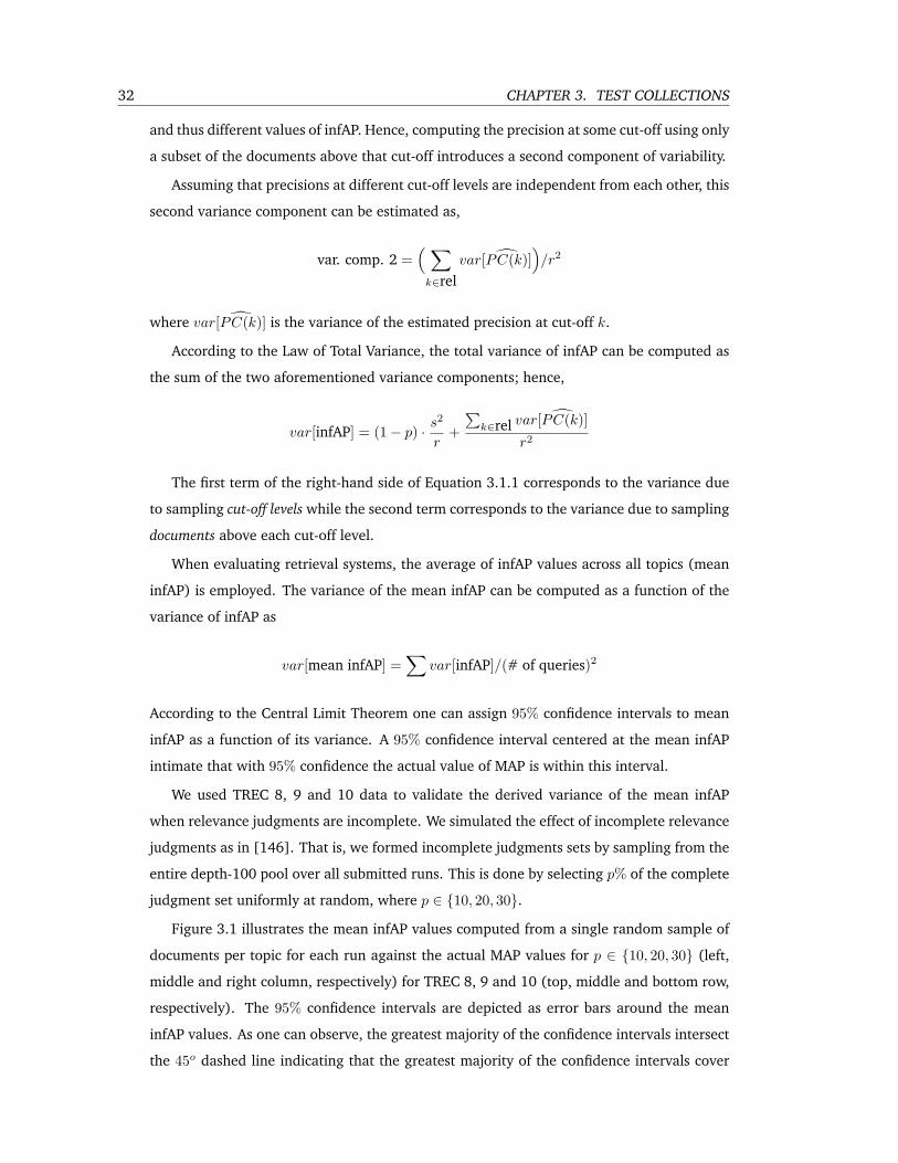
32 CHAPTER 3. TEST COLLECTIONS
and thus different values of infAP. Hence, computing the precision at some cut-off using only
a subset of the documents above that cut-off introduces a second component of variability.
Assuming that precisions at different cut-off levels are independent from each other, this
second variance component can be estimated as,
var. comp. 2 =( ∑
k∈relvar[ PC(k)]
)/r2
where var[ PC(k)] is the variance of the estimated precision at cut-off k.
According to the Law of Total Variance, the total variance of infAP can be computed as
the sum of the two aforementioned variance components; hence,
var[infAP] = (1− p) · s2
r+
∑k∈rel var[ PC(k)]
r2
The first term of the right-hand side of Equation 3.1.1 corresponds to the variance due
to sampling cut-off levels while the second term corresponds to the variance due to sampling
documents above each cut-off level.
When evaluating retrieval systems, the average of infAP values across all topics (mean
infAP) is employed. The variance of the mean infAP can be computed as a function of the
variance of infAP as
var[mean infAP] =∑
var[infAP]/(# of queries)2
According to the Central Limit Theorem one can assign 95% confidence intervals to mean
infAP as a function of its variance. A 95% confidence interval centered at the mean infAP
intimate that with 95% confidence the actual value of MAP is within this interval.
We used TREC 8, 9 and 10 data to validate the derived variance of the mean infAP
when relevance judgments are incomplete. We simulated the effect of incomplete relevance
judgments as in [146]. That is, we formed incomplete judgments sets by sampling from the
entire depth-100 pool over all submitted runs. This is done by selecting p% of the complete
judgment set uniformly at random, where p ∈ {10, 20, 30}.
Figure 3.1 illustrates the mean infAP values computed from a single random sample of
documents per topic for each run against the actual MAP values for p ∈ {10, 20, 30} (left,
middle and right column, respectively) for TREC 8, 9 and 10 (top, middle and bottom row,
respectively). The 95% confidence intervals are depicted as error bars around the mean
infAP values. As one can observe, the greatest majority of the confidence intervals intersect
the 45o dashed line indicating that the greatest majority of the confidence intervals cover
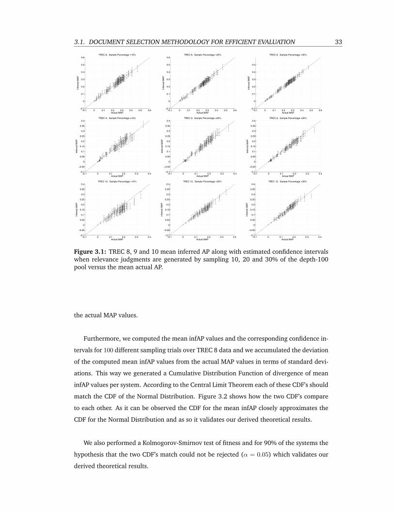
3.1. DOCUMENT SELECTION METHODOLOGY FOR EFFICIENT EVALUATION 33
−0.1 0 0.1 0.2 0.3 0.4 0.5 0.6−0.1
0
0.1
0.2
0.3
0.4
0.5
0.6
Actual MAP
Infe
rred
MA
P
TREC 8, Sample Percentage =10%
−0.1 0 0.1 0.2 0.3 0.4 0.5 0.6−0.1
0
0.1
0.2
0.3
0.4
0.5
0.6
Actual MAP
Infe
rred
MA
P
TREC 8, Sample Percentage =20%
−0.1 0 0.1 0.2 0.3 0.4 0.5 0.6−0.1
0
0.1
0.2
0.3
0.4
0.5
Actual MAP
Infe
rred
MA
P
TREC 8, Sample Percentage =30%
−0.1 0 0.1 0.2 0.3 0.4−0.1
−0.05
0
0.05
0.1
0.15
0.2
0.25
0.3
0.35
0.4
Actual MAP
Infe
rred
MA
P
TREC 9, Sample Percentage =10%
−0.1 0 0.1 0.2 0.3 0.4−0.1
−0.05
0
0.05
0.1
0.15
0.2
0.25
0.3
0.35
0.4
Actual MAP
Infe
rred
MA
P
TREC 9, Sample Percentage =20%
−0.1 0 0.1 0.2 0.3 0.4−0.1
−0.05
0
0.05
0.1
0.15
0.2
0.25
0.3
0.35
0.4
Actual MAP
Infe
rred
MA
P
TREC 9, Sample Percentage =30%
−0.1 0 0.1 0.2 0.3 0.4−0.1
−0.05
0
0.05
0.1
0.15
0.2
0.25
0.3
0.35
0.4
Actual MAP
Infe
rred
MA
P
TREC 10, Sample Percentage =10%
−0.1 0 0.1 0.2 0.3 0.4−0.1
−0.05
0
0.05
0.1
0.15
0.2
0.25
0.3
0.35
0.4
Actual MAP
Infe
rred
MA
P
TREC 10, Sample Percentage =20%
−0.1 0 0.1 0.2 0.3 0.4−0.1
−0.05
0
0.05
0.1
0.15
0.2
0.25
0.3
0.35
0.4
Actual MAP
Infe
rred
MA
P
TREC 10, Sample Percentage =30%
Figure 3.1: TREC 8, 9 and 10 mean inferred AP along with estimated confidence intervalswhen relevance judgments are generated by sampling 10, 20 and 30% of the depth-100pool versus the mean actual AP.
the actual MAP values.
Furthermore, we computed the mean infAP values and the corresponding confidence in-
tervals for 100 different sampling trials over TREC 8 data and we accumulated the deviation
of the computed mean infAP values from the actual MAP values in terms of standard devi-
ations. This way we generated a Cumulative Distribution Function of divergence of mean
infAP values per system. According to the Central Limit Theorem each of these CDF’s should
match the CDF of the Normal Distribution. Figure 3.2 shows how the two CDF’s compare
to each other. As it can be observed the CDF for the mean infAP closely approximates the
CDF for the Normal Distribution and as so it validates our derived theoretical results.
We also performed a Kolmogorov-Smirnov test of fitness and for 90% of the systems the
hypothesis that the two CDF’s match could not be rejected (α = 0.05) which validates our
derived theoretical results.
34 CHAPTER 3. TEST COLLECTIONS
0 5 10 15 200
0.1
0.2
0.3
0.4
0.5
0.6
0.7
0.8
0.9
1
Per
cent
age
of m
ean
infA
P v
alue
s de
viat
ing
from
act
ual M
AP
val
ues
Number of std. dev. mean infAP values deviate from the actual MAP values
TREC 8 − Cumulative Function Destribution of infAP values
CDF for infAP valuesCDF for Normal Distribution
Figure 3.2: Cumulative Distribution Function of the mean infAP values
3.1.2 Inferred AP on Nonrandom Judgments
In the previous section we derived confidence intervals for infAP in a setup where docu-
ments to be judged were a random subset of the entire document collection. Confidence
intervals can be further reduced (i.e. the accuracy of the estimator can be improved) by
utilizing a top-heavy sampling strategy. In this section we consider a setup where relevance
judgments are not a random subset of complete judgments and show how infAP can be
extended to produce unbiased estimates of average precision in such a setup. We denote
the extended infAP measure as xinfAP.
Similar to the infAP paradigm, consider the case where we would like to evaluate the
quality of retrieval systems with respect to a complete pool and assume that relevant judg-
ments are incomplete. Further assume that the set of available judgments are constructed
by dividing the complete collection of documents into disjoint contiguous subsets (strata)
and then randomly selecting (sampling) some documents from each stratum to be judged.
The sampling within each stratum is performed independently, therefore, the sampling per-
centage can be chosen to be different for each stratum. For instance, one could choose to
split the collection of documents into two strata (based on where they appear in the output
of search engines), and sample 90% of the documents from the first stratum and 30% of
3.1. DOCUMENT SELECTION METHODOLOGY FOR EFFICIENT EVALUATION 35
the documents from the second stratum. In effect, one could think a large variety of sam-
pling strategies in terms of this multi-strata strategy. For example, the sampling strategy
proposed by Aslam et al. [5] can be thought as each stratum containing a single document,
with different sampling probabilities assigned to different strata.
Let AP be the random variable corresponding to the estimated average precision of a
system. Now consider the first step of the random experiment whose expectation corre-
sponds to average precision, i.e. picking a relevant document at random. Note that in
the above setup, this relevant document could fall into any one of the different strata s.
Since the sets of documents contained in the strata are disjoint, by definition of conditional
expectation, one can write E[AP ] as:
E[AP ] =∑
∀s∈StrataPs · Es[AP ]
where Ps corresponds to the probability of picking the relevant document from stratum s
and Es[AP ] corresponds to the expected value of average precision given that the relevant
document was picked from stratum s.
Let RQ be the total number of relevant documents in the complete judgment set and
Rs be the total number of relevant documents in stratum s if we were to have all complete
relevance judgments. Then, since selecting documents from different strata is independent
for each stratum, the probability of picking a relevant document from stratum s is, Ps =
Rs/RQ.
Computing the actual values of RQ and Rs is not possible, since the complete set of
judgments is not available. However, we can estimate their values using the incomplete
relevance judgments. Let rs be the number of sampled relevant documents from stratum
s and ns be the total number of sampled documents from stratum s. Furthermore, let Ns
be the total number of documents in stratum s. Since the ns documents were sampled
uniformly from stratum s, the estimated number of relevant documents within stratum s,
Rs, can be computed as Rs = (rs/ns) · Ns. Then the number of relevant documents in
query Q can be estimated as the sum of these estimates over all strata, i.e. RQ =∑∀s Rs.
Given these estimates, the probability of picking a relevant document from stratum s can
be estimated by, Ps = Rs/RQ.
Now, we need to compute the expected value of estimated average precision, Es[AP ], if
we were to pick a relevant document at random from stratum s.
Since the incomplete relevance judgments within each stratum s is a uniform random
subset of the judgments in that stratum, the induced distribution over relevant documents
within each stratum is also uniform, as desired. Therefore, the probability of picking any
36 CHAPTER 3. TEST COLLECTIONS
relevant document within this stratum is equal. Hence, the expected estimated average pre-
cision value within each stratum, Es[AP ], can be computed as the average of the precisions
at judged (sampled) relevant documents within that stratum.
Now consider computing the expected precision at a relevant document at rank k, which
corresponds to the expected outcome of picking a document at or above rank k and out-
putting the binary relevance of the document at this rank (steps 2 and 3 of the random
experiment).
When picking a document at random at or above rank k and outputting the binary
relevance of that document, one of the following two cases may occur. With probability
1/k, we pick the current document, and since this document is by definition relevant the
outcome is 1. With probability (k − 1)/k we pick a document above the current document,
in which case we need to calculate the expected precision (or expected binary relevance)
with respect to the documents above rank k. Thus,
E[ PC(k)] =1k· 1 +
k − 1k
E[PCabove k]
Let Nk−1s be the total number of documents above rank k that belong in stratum s, nk−1
s
be the total number of judged (sampled) documents above rank k that belong to stratum s
and rk−1s be the total number of judged (sampled) relevant documents above rank k that
also belong to stratum s.
When computing the expected precision within the (k − 1) documents above rank k,
with probability Nk−1s /(k − 1) we pick a document from stratum s Therefore, the expected
precision above rank k can be written as:
E[prec above k] =∑∀s
Nk−1s
k − 1· Es[PCabove k
]
where Es[PCabove k] is the expected precision above rank k within stratum s. Since we
have a uniform sample of judged documents from stratum s, we can use these sampled
documents to estimate the expected precision within stratum s. Since the incomplete rele-
vance judgments from each stratum is obtained by uniform random sampling, this expected
precision can be computed as rk−1s /nk−1
s .
Note that in computing the expected precision in stratum s, we may face the problem
of not having sampled any documents from this stratum that are above the current rel-
evant document at rank k. Adapting the same idea used in infAP, we employ Lindstone
smoothing [37] to avoid this problem. Therefore, expected precision above rank k can be
3.1. DOCUMENT SELECTION METHODOLOGY FOR EFFICIENT EVALUATION 37
computed as:
E[PCabove k] =
∑∀s
Nk−1s
k − 1· rk−1
s + ε
nk−1s + 2ε
It is easy to see that when complete judgments are available, xinfAP is exactly equal to
average precision (ignoring the smoothing effect). Further, note that infAP is a particular
instantiation of this formula with a single stratum used.
Overall, the advantage and real power of the described stratified random sampling and
the derived AP estimator, xinfAP, is the fact that it combines the effectiveness of the sam-
pling method proposed by Aslam et al. [5] by employing stratification of the documents
and thus better utilization of the judgment effort with the simplicity of infAP by employing
random sampling within each stratum.
3.1.3 Inferred AP in TREC Terabyte
As mentioned, xinfAP can be used with a large variety of sampling strategy. In this section,
we focus on the sampling strategy used in TREC Terabyte 2006 [28] and we show that
(1) xinfAP is highly effective at estimating average precision and (2) it better utilizes the
judgment effort compared to infAP.
First, let’s briefly consider the sampling strategy used in TREC Terabyte 2006. In this
track, three different sets of relevance judgments were formed, with only two of them being
used for evaluation purposes. Out of these two sets, the first set of judgments, constructed
by the traditional depth-50 pooling strategy, was used to obtain a rough idea of the systems
average precision. The second set of judgments was constructed using random sampling
in such a way that there are more documents judged from topics that are more likely to
have retrieved more relevant documents. Since, in Terabyte track, the size of the document
collection is very large, the systems may continue retrieving relevant documents even at
high ranks (deeper in the list). This set of judgments was created to obtain an estimate of
average precision if complete judgments were present.
To estimate average precision, infAP was used as the evaluation measure. Since, by
design, infAP assumes that the set of relevance judgments is a random subset of complete
judgments, even though the entire depth-50 pool was judged, infAP was computed only
using the random sample of judgments (second set) without utilizing judgments from the
depth-50 pool. Therefore, many relevance judgments were not used even though they were
available.
Note that xinfAP can easily handle this setup and it could be used to utilize all the
judgments, obtaining better estimates of average precision.
38 CHAPTER 3. TEST COLLECTIONS
To test how xinfAP compares with infAP we simulate the sampling strategy used in TREC
Terabyte 06 on data from TREC 8. The TREC Terabyte data was not used due to the fact
that in TREC Terabyte the actual value of average precision is not known since ”complete”
judgments are not available.
To simulate the setup used in TREC Terabyte, we first form different depth-k pools
where k ∈ {1, 2, 3, 4, 5, 10, 20, 30, 40, 50} and obtain judgments for all documents in each
one of these pools. Then, for each value of k, we compute the total number of documents
that are in the depth-k pool and we randomly sample equal number of documents from
the complete judgment set2 excluding the depth-k pool. After forming these two sets of
judgments (depth-k and random) we combine them and compute xinfAP on these combined
judgments.
This setup exactly corresponds to a sampling strategy where complete judgments are
divided into two strata and judgments are formed by uniformly and independently sampling
within each stratum.
Note that in TREC, there are some systems that were submitted but that did not con-
tribute to the pool. To further evaluate the quality of our estimators in terms of their
robustness for evaluating the quality of unseen systems (systems that did not contribute to
the pool), when we form the incomplete relevance judgments, we only consider the systems
that contribute to the pool but we compute the xinfAP estimates for all submitted systems.
Figure 3.3 demonstrates how xinfAP computed using judgments generated by combining
depth-10 (top row, left), depth-5 (top row, right) and depth-1 (bottom row) pools with
equal number of randomly sampled judgments compares with the actual AP. Each of these
depths correspond to judging 23.1%, 12.7% and 3.5% of the entire pool, respectively. The
plots report the RMS error (how accurate are the estimated values?), the Kendall’s τ value
(how accurate are the estimated rankings of systems?) and the linear correlation coefficient,
ρ, (how well do the estimated values fit in a straight line compared to the actual values?). 3
The dot signs in the figures refer to the systems that were used to create the original pools
and the plus signs refer to the systems that did not contribute to the pool.
The results illustrated in these plots reinforce our claims that xinfAP is an unbiased
estimator of average precision. Furthermore, it can be seen that the measure can reliably
be used to evaluate the quality of systems that were not used to create the initial samples,
hence the measure is robust to evaluating the quality of unseen systems.
Figure 3.4 illustrates how xinfAP computed on a non-random judgment set compares
with infAP computed on a random judgment set for various levels of incompleteness. In a
2Throughout this section, we assume that the complete judgment set corresponds to the depth-100 pool as thejudgments we have are formed using depth-100 pools and assuming the remaining documents are nonrelevant.
3A more detailed description of these statistics is given in Appendix C.
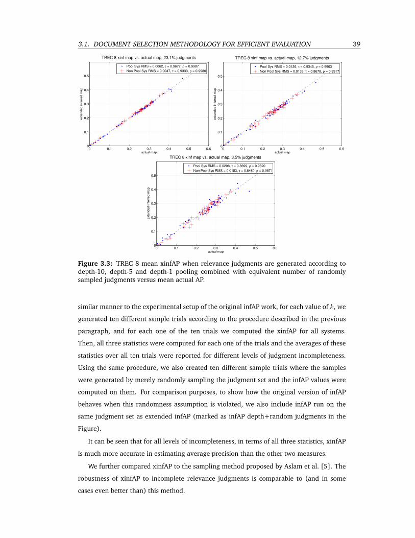
3.1. DOCUMENT SELECTION METHODOLOGY FOR EFFICIENT EVALUATION 39
0 0.1 0.2 0.3 0.4 0.5 0.60
0.1
0.2
0.3
0.4
0.5
actual map
exte
nd
ed
in
ferr
ed
ma
p
TREC 8 xinf map vs. actual map, 12.7% judgments
Pool Sys RMS = 0.0126, τ = 0.9345, ρ = 0.9963
Non Pool Sys RMS = 0.0133, τ = 0.8678, ρ = 0.9917
0 0.1 0.2 0.3 0.4 0.5 0.60
0.1
0.2
0.3
0.4
0.5
actual map
exte
nd
ed
in
ferr
ed
ma
p
TREC 8 xinf map vs. actual map, 3.5% judgments
Pool Sys RMS = 0.0206, τ = 0.8699, ρ = 0.9820
Non Pool Sys RMS = 0.0153, τ = 0.8480, ρ = 0.9871
Figure 3.3: TREC 8 mean xinfAP when relevance judgments are generated according todepth-10, depth-5 and depth-1 pooling combined with equivalent number of randomlysampled judgments versus mean actual AP.
similar manner to the experimental setup of the original infAP work, for each value of k, we
generated ten different sample trials according to the procedure described in the previous
paragraph, and for each one of the ten trials we computed the xinfAP for all systems.
Then, all three statistics were computed for each one of the trials and the averages of these
statistics over all ten trials were reported for different levels of judgment incompleteness.
Using the same procedure, we also created ten different sample trials where the samples
were generated by merely randomly sampling the judgment set and the infAP values were
computed on them. For comparison purposes, to show how the original version of infAP
behaves when this randomness assumption is violated, we also include infAP run on the
same judgment set as extended infAP (marked as infAP depth+random judgments in the
Figure).
It can be seen that for all levels of incompleteness, in terms of all three statistics, xinfAP
is much more accurate in estimating average precision than the other two measures.
We further compared xinfAP to the sampling method proposed by Aslam et al. [5]. The
robustness of xinfAP to incomplete relevance judgments is comparable to (and in some
cases even better than) this method.
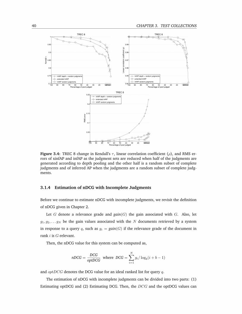
40 CHAPTER 3. TEST COLLECTIONS
1234567891020304050607080901000.7
0.75
0.8
0.85
0.9
0.95
1
Percentage of pool judged
Ken
dall
τ
TREC 8
InfAP depth + random judgments
extended InfAP
InfAP random judgments
1234567891020304050607080901000.94
0.95
0.96
0.97
0.98
0.99
1
Percentage of pool judged
Line
ar c
orre
latio
n co
effic
ient
(ρ)
TREC 8
InfAP depth + random judgments
extended InfAP
InfAP random judgments
1234567891020304050607080901000
0.05
0.1
0.15
0.2
0.25
Percentage of pool judged
RM
S e
rror
TREC 8
InfAP depth + random judgments
extended infAP
InfAP random judgments
Figure 3.4: TREC 8 change in Kendall’s τ , linear correlation coefficient (ρ), and RMS er-rors of xinfAP and infAP as the judgment sets are reduced when half of the judgments aregenerated according to depth pooling and the other half is a random subset of completejudgments and of inferred AP when the judgments are a random subset of complete judg-ments.
3.1.4 Estimation of nDCG with Incomplete Judgments
Before we continue to estimate nDCG with incomplete judgments, we revisit the definition
of nDCG given in Chapter 2.
Let G denote a relevance grade and gain(G) the gain associated with G. Also, let
g1, g2, . . . gN be the gain values associated with the N documents retrieved by a system
in response to a query q, such as gi = gain(G) if the relevance grade of the document in
rank i is G-relevant.
Then, the nDCG value for this system can be computed as,
nDCG =DCG
optDCGwhere DCG =
N∑i=1
gi/ logb(i + b− 1)
and optDCG denotes the DCG value for an ideal ranked list for query q.
The estimation of nDCG with incomplete judgments can be divided into two parts: (1)
Estimating optDCG and (2) Estimating DCG. Then, the DCG and the optDCG values can
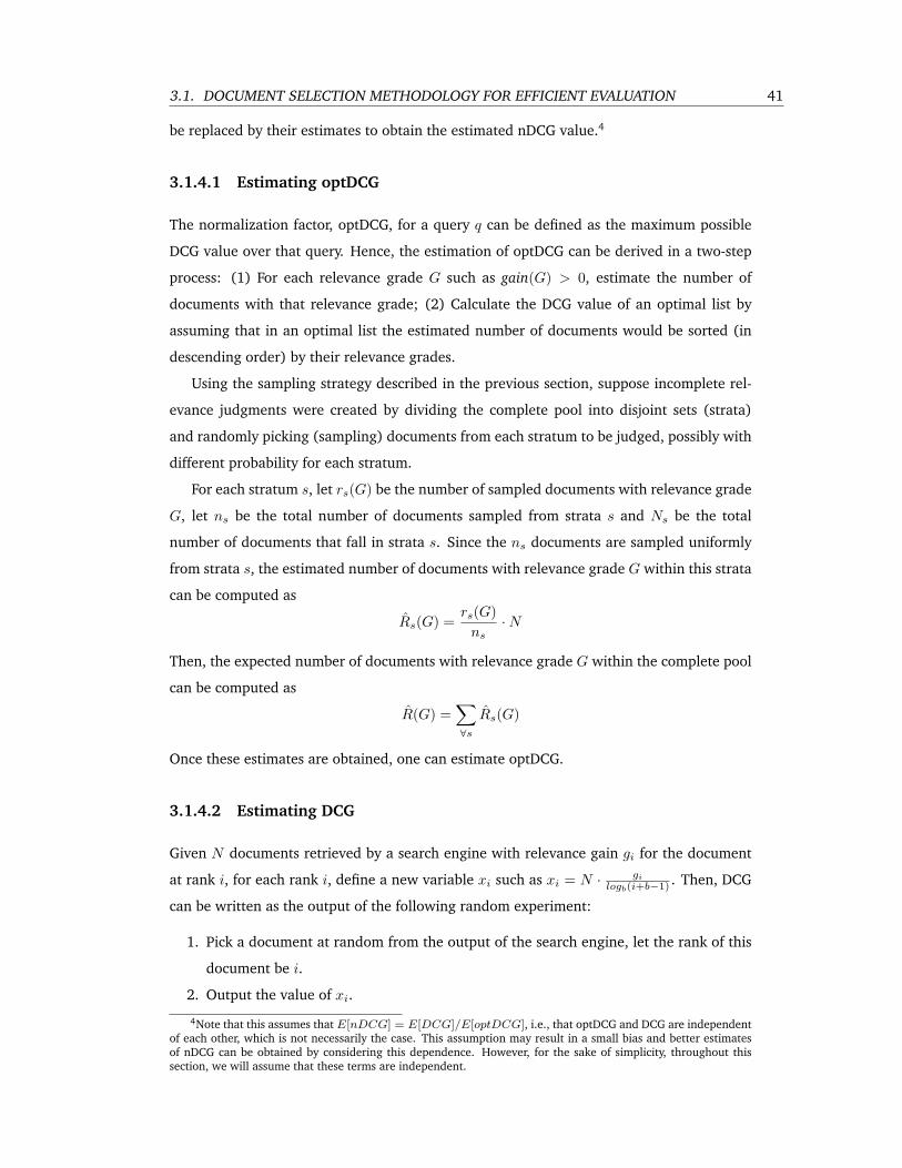
3.1. DOCUMENT SELECTION METHODOLOGY FOR EFFICIENT EVALUATION 41
be replaced by their estimates to obtain the estimated nDCG value.4
3.1.4.1 Estimating optDCG
The normalization factor, optDCG, for a query q can be defined as the maximum possible
DCG value over that query. Hence, the estimation of optDCG can be derived in a two-step
process: (1) For each relevance grade G such as gain(G) > 0, estimate the number of
documents with that relevance grade; (2) Calculate the DCG value of an optimal list by
assuming that in an optimal list the estimated number of documents would be sorted (in
descending order) by their relevance grades.
Using the sampling strategy described in the previous section, suppose incomplete rel-
evance judgments were created by dividing the complete pool into disjoint sets (strata)
and randomly picking (sampling) documents from each stratum to be judged, possibly with
different probability for each stratum.
For each stratum s, let rs(G) be the number of sampled documents with relevance grade
G, let ns be the total number of documents sampled from strata s and Ns be the total
number of documents that fall in strata s. Since the ns documents are sampled uniformly
from strata s, the estimated number of documents with relevance grade G within this strata
can be computed as
Rs(G) =rs(G)
ns·N
Then, the expected number of documents with relevance grade G within the complete pool
can be computed as
R(G) =∑∀s
Rs(G)
Once these estimates are obtained, one can estimate optDCG.
3.1.4.2 Estimating DCG
Given N documents retrieved by a search engine with relevance gain gi for the document
at rank i, for each rank i, define a new variable xi such as xi = N · gi
logb(i+b−1) . Then, DCG
can be written as the output of the following random experiment:
1. Pick a document at random from the output of the search engine, let the rank of this
document be i.
2. Output the value of xi.
4Note that this assumes that E[nDCG] = E[DCG]/E[optDCG], i.e., that optDCG and DCG are independentof each other, which is not necessarily the case. This assumption may result in a small bias and better estimatesof nDCG can be obtained by considering this dependence. However, for the sake of simplicity, throughout thissection, we will assume that these terms are independent.
42 CHAPTER 3. TEST COLLECTIONS
It is easy to see that if we have the relevance judgments for all N documents, the ex-
pected value of this random experiment is exactly equal to DCG.
Now consider estimating the outcome of this random experiment when relevance judg-
ments are incomplete. Consider the first step of the random experiment, i.e. picking a
document at random. Let Ns be the number of documents in the output of a system that
fall in stratum s. When picking a document at random, with probability Ns/N , we pick a
document from stratum s.
Therefore, the expected value of the above random experiment can be written as:
E[DCG] =∑∀s
Ns
N· E[xi|document at rank i ∈ s]
Now consider the second step of the random experiment, computing the expected value of
xi given that the document at rank i falls in strata s. Let sampleds be the set of sampled
documents from strata s and ns be the number of documents sampled from this strata.
Since documents within stratum s are uniformly sampled, the expected value of xi can be
computed as
E[xi|document at rank i ∈ s] =1ns
∑∀j∈sampleds
xj
Once E[optDCG] and E[DCG] are computed, infNDCG can then be computed as infNDCG
= E[DCG]/E[optDCG].
3.1.5 Overall Results
Until now, we have shown that using a similar sampling strategy as the one used in TREC
Terabyte 06 (complete judgments divided into 2 different strata), xinfAP is highly accurate.
In this section, we show that (1) this claim is consistent over different TRECs for both xinfAP
and infNDCG and that (2) the two measures can be used with the complete judgments
divided into more than two strata.
In order to check (2), we use a different sampling strategy than the one in Terabyte; we
divide the complete judgment set (assuming depth-100 pool is the complete judgment set)
into 4 different strata. The first stratum is the regular depth-k pool, fully judged. Instead of
randomly sampling equal to the depth-k pool number of judgments from the remainder of
the collection, we now divide the rest of the documents into three other strata and distribute
the remaining judgments with a ratio of 3:1.5:1 (judge 55% of the documents in the top
depth stratum, 27% of the documents in the middle depth stratum and 18% in the lowest
depth stratum). This way, more weight is given to judging documents retrieved towards the
top of the ranked lists of the search engines. Note, however, that as the number of strata
3.1. DOCUMENT SELECTION METHODOLOGY FOR EFFICIENT EVALUATION 43
1234510152025304050607080901000.7
0.75
0.8
0.85
0.9
0.95
1TREC 8
percentage of pool judged
Ken
dall
τ
extended InfAPextended infNDCGinfAPNDCG random
1234510152025304050607080901000.75
0.8
0.85
0.9
0.95
1TREC 9
percentage of pool judged
Ken
dall
τ
extended InfAPextended infNDCGinfAPNDCG random
1234510152025304050607080901000.65
0.7
0.75
0.8
0.85
0.9
0.95
1TREC 10
percentage of pool judged
Ken
dall
τ
extended InfAPextended infNDCGinfAPNDCG random
Figure 3.5: Comparison of extended inferred map, (extended) mean inferred nDCG, in-ferred map and mean nDCG on random judgments, using Kendall’s τ for TREC 8, 9 and10.
increase, there values of the estimates may slightly deviate from the actual values since the
effect of smoothing also increase (smoothing is needed for each stratum).
Figures 3.5, 3.6 and 3.7 show the quality of xinfAP and infNDCG (referred as extended
infNDCG to avoid confusion) computed on these samples according to Kendall’s τ , linear
correlation coefficient (ρ) and RMS Error statistics, respectively, for TRECs 8, 9 and 10.
For comparison purposes, the plots also contain infAP and nDCG (the standard formula
computed on random judgments, assuming unjudged documents are nonrelevant).
Looking at all plots, it can be seen that according to both statistics, using the same
number of judgments, the extended infAP (xinfAP) and infNDCG consistently outperform
infAP and nDCG on random judgments, respectively. The high RMS error of nDCG on
random judgments is due to the fact that nDCG is computed on these judgments as it is,
without aiming at estimating the value of the measure.
3.1.6 Conclusions
In this work, we extended inferred AP in two different ways. First, we derived confidence
intervals for infAP to capture the variability in infAP values. Employing confidence intervals
enables comparisons and eventually ranking of systems according to their quality measured
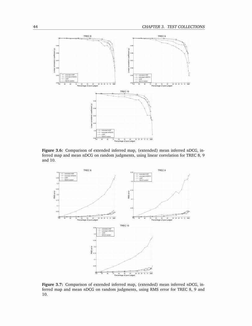
44 CHAPTER 3. TEST COLLECTIONS
1234510152025304050607080901000.94
0.95
0.96
0.97
0.98
0.99
1TREC 8
Percentage of pool judged
Line
ar c
orre
latio
n co
effic
ient
(ρ)
extended InfAPextended infNDCGinfAPNDCG random
1234510152025304050607080901000.94
0.95
0.96
0.97
0.98
0.99
1TREC 9
Percentage of pool judged
Line
ar c
orre
latio
n co
effic
ient
(ρ)
extended InfAPextended infNDCGinfAPNDCG random
1234510152025304050607080901000.88
0.9
0.92
0.94
0.96
0.98
1TREC 10
Percentage of pool judged
Line
ar c
orre
latio
n co
effic
ient
(ρ)
extended InfAPextended infNDCGinfAPNDCG random
Figure 3.6: Comparison of extended inferred map, (extended) mean inferred nDCG, in-ferred map and mean nDCG on random judgments, using linear correlation for TREC 8, 9and 10.
1234510152025304050607080901000
0.05
0.1
0.15
0.2
0.25
0.3
0.35
0.4TREC 8
Percentage of pool judged
RM
S e
rror
extended InfAPextended infNDCGinfAPNDCG random
1234510152025304050607080901000
0.05
0.1
0.15
0.2
0.25TREC 9
Percentage of pool judged
RM
S e
rror
extended InfAPextended infNDCGinfAPNDCG random
1234510152025304050607080901000
0.05
0.1
0.15
0.2
0.25
0.3
0.35TREC 10
Percentage of pool judged
RM
S e
rror
extended InfAPextended infNDCGinfAPNDCG random
Figure 3.7: Comparison of extended inferred map, (extended) mean inferred nDCG, in-ferred map and mean nDCG on random judgments, using RMS error for TREC 8, 9 and10.
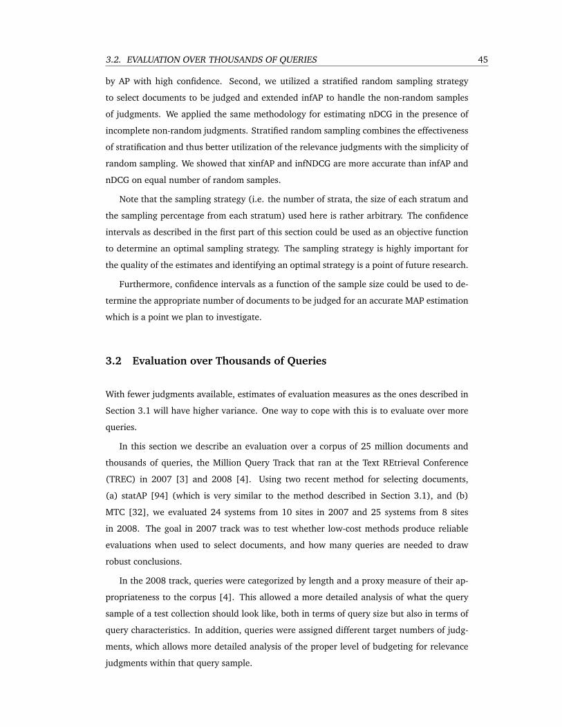
3.2. EVALUATION OVER THOUSANDS OF QUERIES 45
by AP with high confidence. Second, we utilized a stratified random sampling strategy
to select documents to be judged and extended infAP to handle the non-random samples
of judgments. We applied the same methodology for estimating nDCG in the presence of
incomplete non-random judgments. Stratified random sampling combines the effectiveness
of stratification and thus better utilization of the relevance judgments with the simplicity of
random sampling. We showed that xinfAP and infNDCG are more accurate than infAP and
nDCG on equal number of random samples.
Note that the sampling strategy (i.e. the number of strata, the size of each stratum and
the sampling percentage from each stratum) used here is rather arbitrary. The confidence
intervals as described in the first part of this section could be used as an objective function
to determine an optimal sampling strategy. The sampling strategy is highly important for
the quality of the estimates and identifying an optimal strategy is a point of future research.
Furthermore, confidence intervals as a function of the sample size could be used to de-
termine the appropriate number of documents to be judged for an accurate MAP estimation
which is a point we plan to investigate.
3.2 Evaluation over Thousands of Queries
With fewer judgments available, estimates of evaluation measures as the ones described in
Section 3.1 will have higher variance. One way to cope with this is to evaluate over more
queries.
In this section we describe an evaluation over a corpus of 25 million documents and
thousands of queries, the Million Query Track that ran at the Text REtrieval Conference
(TREC) in 2007 [3] and 2008 [4]. Using two recent method for selecting documents,
(a) statAP [94] (which is very similar to the method described in Section 3.1), and (b)
MTC [32], we evaluated 24 systems from 10 sites in 2007 and 25 systems from 8 sites
in 2008. The goal in 2007 track was to test whether low-cost methods produce reliable
evaluations when used to select documents, and how many queries are needed to draw
robust conclusions.
In the 2008 track, queries were categorized by length and a proxy measure of their ap-
propriateness to the corpus [4]. This allowed a more detailed analysis of what the query
sample of a test collection should look like, both in terms of query size but also in terms of
query characteristics. In addition, queries were assigned different target numbers of judg-
ments, which allows more detailed analysis of the proper level of budgeting for relevance
judgments within that query sample.
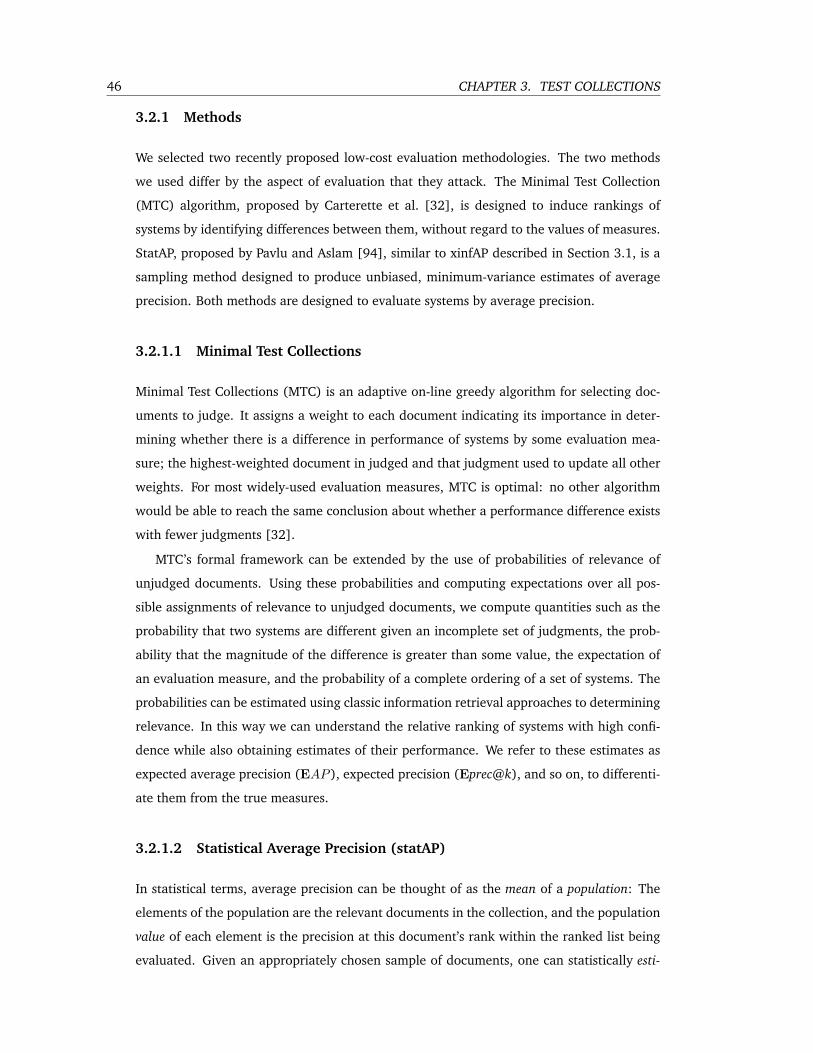
46 CHAPTER 3. TEST COLLECTIONS
3.2.1 Methods
We selected two recently proposed low-cost evaluation methodologies. The two methods
we used differ by the aspect of evaluation that they attack. The Minimal Test Collection
(MTC) algorithm, proposed by Carterette et al. [32], is designed to induce rankings of
systems by identifying differences between them, without regard to the values of measures.
StatAP, proposed by Pavlu and Aslam [94], similar to xinfAP described in Section 3.1, is a
sampling method designed to produce unbiased, minimum-variance estimates of average
precision. Both methods are designed to evaluate systems by average precision.
3.2.1.1 Minimal Test Collections
Minimal Test Collections (MTC) is an adaptive on-line greedy algorithm for selecting doc-
uments to judge. It assigns a weight to each document indicating its importance in deter-
mining whether there is a difference in performance of systems by some evaluation mea-
sure; the highest-weighted document in judged and that judgment used to update all other
weights. For most widely-used evaluation measures, MTC is optimal: no other algorithm
would be able to reach the same conclusion about whether a performance difference exists
with fewer judgments [32].
MTC’s formal framework can be extended by the use of probabilities of relevance of
unjudged documents. Using these probabilities and computing expectations over all pos-
sible assignments of relevance to unjudged documents, we compute quantities such as the
probability that two systems are different given an incomplete set of judgments, the prob-
ability that the magnitude of the difference is greater than some value, the expectation of
an evaluation measure, and the probability of a complete ordering of a set of systems. The
probabilities can be estimated using classic information retrieval approaches to determining
relevance. In this way we can understand the relative ranking of systems with high confi-
dence while also obtaining estimates of their performance. We refer to these estimates as
expected average precision (EAP ), expected precision (Eprec@k), and so on, to differenti-
ate them from the true measures.
3.2.1.2 Statistical Average Precision (statAP)
In statistical terms, average precision can be thought of as the mean of a population: The
elements of the population are the relevant documents in the collection, and the population
value of each element is the precision at this document’s rank within the ranked list being
evaluated. Given an appropriately chosen sample of documents, one can statistically esti-
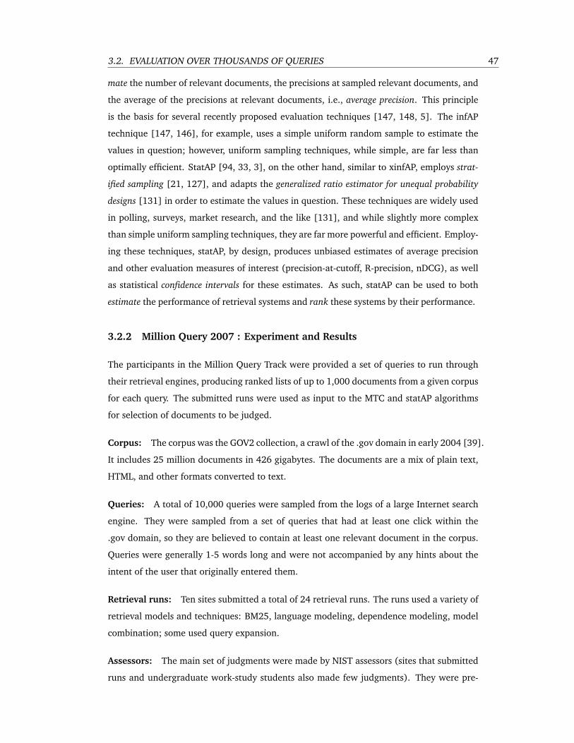
3.2. EVALUATION OVER THOUSANDS OF QUERIES 47
mate the number of relevant documents, the precisions at sampled relevant documents, and
the average of the precisions at relevant documents, i.e., average precision. This principle
is the basis for several recently proposed evaluation techniques [147, 148, 5]. The infAP
technique [147, 146], for example, uses a simple uniform random sample to estimate the
values in question; however, uniform sampling techniques, while simple, are far less than
optimally efficient. StatAP [94, 33, 3], on the other hand, similar to xinfAP, employs strat-
ified sampling [21, 127], and adapts the generalized ratio estimator for unequal probability
designs [131] in order to estimate the values in question. These techniques are widely used
in polling, surveys, market research, and the like [131], and while slightly more complex
than simple uniform sampling techniques, they are far more powerful and efficient. Employ-
ing these techniques, statAP, by design, produces unbiased estimates of average precision
and other evaluation measures of interest (precision-at-cutoff, R-precision, nDCG), as well
as statistical confidence intervals for these estimates. As such, statAP can be used to both
estimate the performance of retrieval systems and rank these systems by their performance.
3.2.2 Million Query 2007 : Experiment and Results
The participants in the Million Query Track were provided a set of queries to run through
their retrieval engines, producing ranked lists of up to 1,000 documents from a given corpus
for each query. The submitted runs were used as input to the MTC and statAP algorithms
for selection of documents to be judged.
Corpus: The corpus was the GOV2 collection, a crawl of the .gov domain in early 2004 [39].
It includes 25 million documents in 426 gigabytes. The documents are a mix of plain text,
HTML, and other formats converted to text.
Queries: A total of 10,000 queries were sampled from the logs of a large Internet search
engine. They were sampled from a set of queries that had at least one click within the
.gov domain, so they are believed to contain at least one relevant document in the corpus.
Queries were generally 1-5 words long and were not accompanied by any hints about the
intent of the user that originally entered them.
Retrieval runs: Ten sites submitted a total of 24 retrieval runs. The runs used a variety of
retrieval models and techniques: BM25, language modeling, dependence modeling, model
combination; some used query expansion.
Assessors: The main set of judgments were made by NIST assessors (sites that submitted
runs and undergraduate work-study students also made few judgments). They were pre-
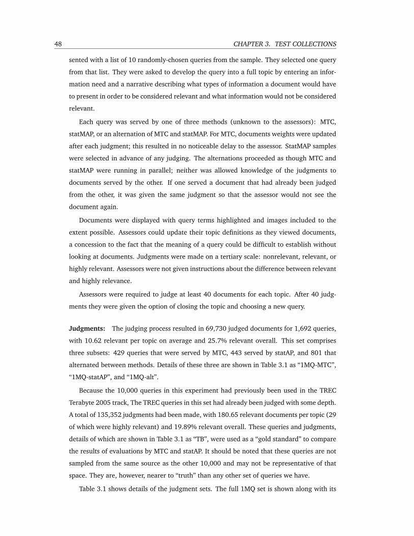
48 CHAPTER 3. TEST COLLECTIONS
sented with a list of 10 randomly-chosen queries from the sample. They selected one query
from that list. They were asked to develop the query into a full topic by entering an infor-
mation need and a narrative describing what types of information a document would have
to present in order to be considered relevant and what information would not be considered
relevant.
Each query was served by one of three methods (unknown to the assessors): MTC,
statMAP, or an alternation of MTC and statMAP. For MTC, documents weights were updated
after each judgment; this resulted in no noticeable delay to the assessor. StatMAP samples
were selected in advance of any judging. The alternations proceeded as though MTC and
statMAP were running in parallel; neither was allowed knowledge of the judgments to
documents served by the other. If one served a document that had already been judged
from the other, it was given the same judgment so that the assessor would not see the
document again.
Documents were displayed with query terms highlighted and images included to the
extent possible. Assessors could update their topic definitions as they viewed documents,
a concession to the fact that the meaning of a query could be difficult to establish without
looking at documents. Judgments were made on a tertiary scale: nonrelevant, relevant, or
highly relevant. Assessors were not given instructions about the difference between relevant
and highly relevance.
Assessors were required to judge at least 40 documents for each topic. After 40 judg-
ments they were given the option of closing the topic and choosing a new query.
Judgments: The judging process resulted in 69,730 judged documents for 1,692 queries,
with 10.62 relevant per topic on average and 25.7% relevant overall. This set comprises
three subsets: 429 queries that were served by MTC, 443 served by statAP, and 801 that
alternated between methods. Details of these three are shown in Table 3.1 as “1MQ-MTC”,
“1MQ-statAP”, and “1MQ-alt”.
Because the 10,000 queries in this experiment had previously been used in the TREC
Terabyte 2005 track, The TREC queries in this set had already been judged with some depth.
A total of 135,352 judgments had been made, with 180.65 relevant documents per topic (29
of which were highly relevant) and 19.89% relevant overall. These queries and judgments,
details of which are shown in Table 3.1 as “TB”, were used as a “gold standard” to compare
the results of evaluations by MTC and statAP. It should be noted that these queries are not
sampled from the same source as the other 10,000 and may not be representative of that
space. They are, however, nearer to “truth” than any other set of queries we have.
Table 3.1 shows details of the judgment sets. The full 1MQ set is shown along with its
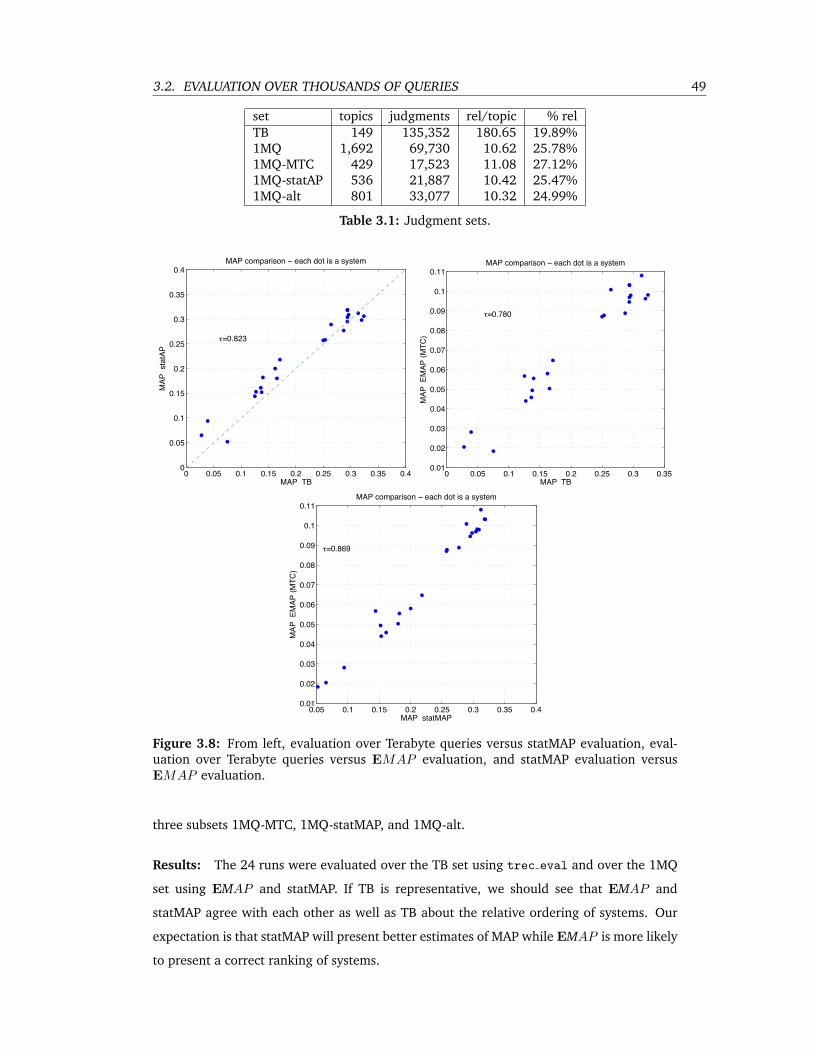
3.2. EVALUATION OVER THOUSANDS OF QUERIES 49
set topics judgments rel/topic % relTB 149 135,352 180.65 19.89%1MQ 1,692 69,730 10.62 25.78%1MQ-MTC 429 17,523 11.08 27.12%1MQ-statAP 536 21,887 10.42 25.47%1MQ-alt 801 33,077 10.32 24.99%
Table 3.1: Judgment sets.
0 0.05 0.1 0.15 0.2 0.25 0.3 0.35 0.40
0.05
0.1
0.15
0.2
0.25
0.3
0.35
0.4
MAP TB
MAP
sta
tAP
MAP comparison ! each dot is a system
!=0.823
0 0.05 0.1 0.15 0.2 0.25 0.3 0.350.01
0.02
0.03
0.04
0.05
0.06
0.07
0.08
0.09
0.1
0.11
MAP TB
MAP
2M
AP 3M
TC5
MAP comparison ! each dot is a system
!=0.780
0.05 0.1 0.15 0.2 0.25 0.3 0.35 0.40.01
0.02
0.03
0.04
0.05
0.06
0.07
0.08
0.09
0.1
0.11
MAP statMAP
MAP
3M
AP 4M
TC7
MAP comparison ! each dot is a system
!=0.869
Figure 3.8: From left, evaluation over Terabyte queries versus statMAP evaluation, eval-uation over Terabyte queries versus EMAP evaluation, and statMAP evaluation versusEMAP evaluation.
three subsets 1MQ-MTC, 1MQ-statMAP, and 1MQ-alt.
Results: The 24 runs were evaluated over the TB set using trec eval and over the 1MQ
set using EMAP and statMAP. If TB is representative, we should see that EMAP and
statMAP agree with each other as well as TB about the relative ordering of systems. Our
expectation is that statMAP will present better estimates of MAP while EMAP is more likely
to present a correct ranking of systems.

50 CHAPTER 3. TEST COLLECTIONS
Overall, the rankings by EMAP and statMAP are fairly similar, and both are similar
to the ”gold standard”. Figure 3.8 shows how statMAP, EMAP , and MAP over TB queries
correlate. All three methods have identified the same three clusters of systems; within those
clusters there is some variation in the rankings between methods. For statMAP estimates
(Figure 3.8, top row, left plot), besides the ranking correlation, we note the accuracy in
terms of absolute difference with the TB MAP values by the line corresponding to the main
diagonal.
The agreement between the two low-cost methods, which are radically different in terms
of the documents they select to be judged, as well as the high correlation between these
methods and the TB evaluation indicates that sampling a small set of documents per query
can still lead to reliable evaluation, as it was suggested in Section 3.1.
3.2.3 Million Query 2007 : Analysis
As described earlier, the performance of each system per topic is expressed in terms of
average precision of the output list of documents while the overall quality of a system is
captured by averaging its AP values over all topics into its mean average precision. Systems
are then ranked by their MAP scores.
Hypothetically, if a second set of topics was available, the systems could be run over this
new set of topics and new MAP scores (and consequently a new ranking of the systems)
would be produced. Naturally, two questions arise: (1) how do MAP scores or a ranking
of systems over different set of topics compare to each other, and (2) how many topics
are needed to guarantee that the MAP scores or a ranking of systems reflect their actual
performance?
We describe an efficiency study, based on analysis of variance (ANOVA), of the stability of
rankings induced by subsets of queries. Appendix B gives a detailed description on analysis
of variance and variance decomposition.
3.2.3.1 Analysis of Variance Studies
We ran two separate analysis of variance studies; one over the MAP scores estimated by
the MTC method given the set of 429 topics exclusively selected by MTC and one over the
MAP scores estimated by the statAP method over the set of 459 topics exclusively selected
by statAP (both methods utilized 40 relevance judgments per topic). For both studies we
reported (a) the ratio of the variance due to system and the total variance and (b) the ratio
of the variance due to system and the variance components that affect the relative MAP
scores (i.e. the ranking of systems), both as a function of the number of topics in the topics
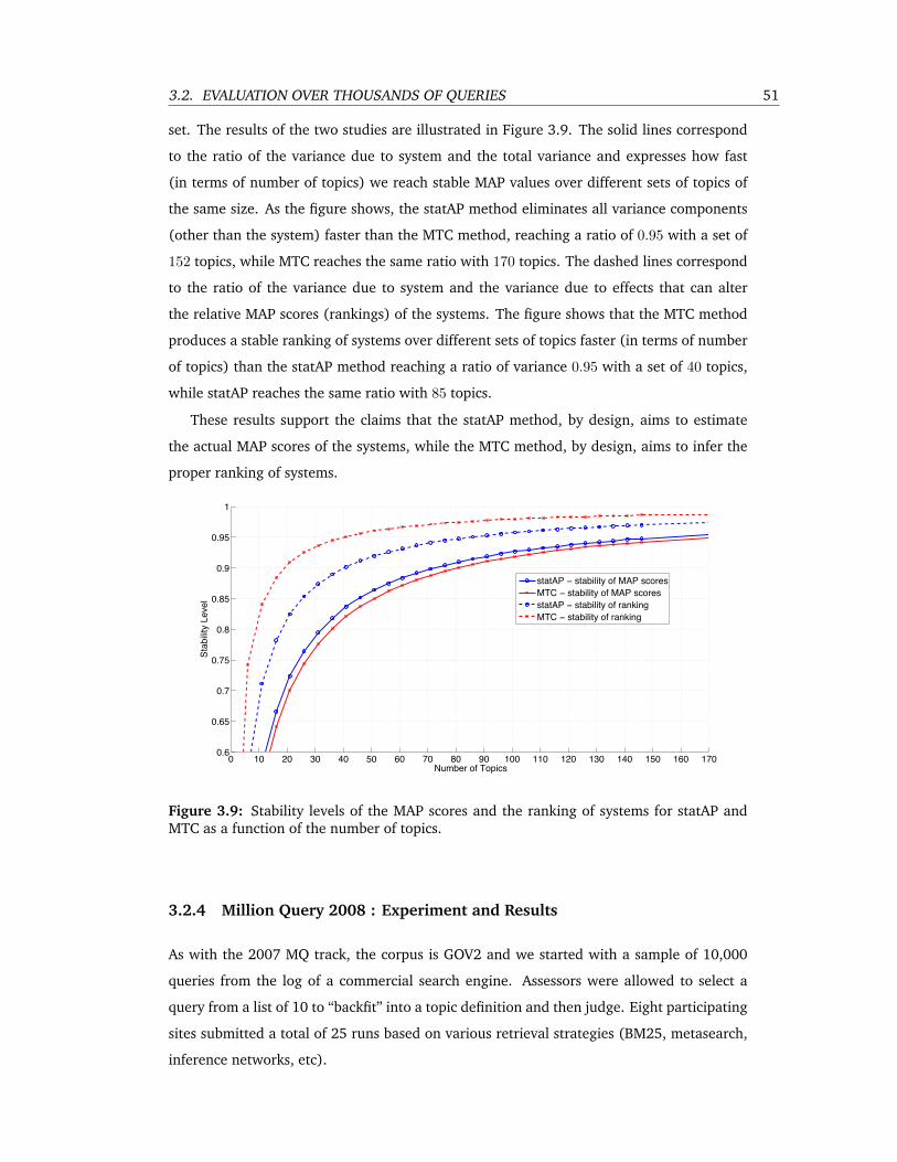
3.2. EVALUATION OVER THOUSANDS OF QUERIES 51
set. The results of the two studies are illustrated in Figure 3.9. The solid lines correspond
to the ratio of the variance due to system and the total variance and expresses how fast
(in terms of number of topics) we reach stable MAP values over different sets of topics of
the same size. As the figure shows, the statAP method eliminates all variance components
(other than the system) faster than the MTC method, reaching a ratio of 0.95 with a set of
152 topics, while MTC reaches the same ratio with 170 topics. The dashed lines correspond
to the ratio of the variance due to system and the variance due to effects that can alter
the relative MAP scores (rankings) of the systems. The figure shows that the MTC method
produces a stable ranking of systems over different sets of topics faster (in terms of number
of topics) than the statAP method reaching a ratio of variance 0.95 with a set of 40 topics,
while statAP reaches the same ratio with 85 topics.
These results support the claims that the statAP method, by design, aims to estimate
the actual MAP scores of the systems, while the MTC method, by design, aims to infer the
proper ranking of systems.
0 10 20 $0 40 50 60 70 80 90 100 110 120 1$0 140 150 160 1700.6
0.65
0.7
0.75
0.8
0.85
0.9
0.95
1
Number of Topics
Stab
ility
Leve
l
statAP ! stability of MAP scoresMTC ! stability of MAP scoresstatAP ! stability of rankingMTC ! stability of ranking
Figure 3.9: Stability levels of the MAP scores and the ranking of systems for statAP andMTC as a function of the number of topics.
3.2.4 Million Query 2008 : Experiment and Results
As with the 2007 MQ track, the corpus is GOV2 and we started with a sample of 10,000
queries from the log of a commercial search engine. Assessors were allowed to select a
query from a list of 10 to “backfit” into a topic definition and then judge. Eight participating
sites submitted a total of 25 runs based on various retrieval strategies (BM25, metasearch,
inference networks, etc).
52 CHAPTER 3. TEST COLLECTIONS
judgment targetcategory 8 16 32 64 128 totalshort-govslant 95 (7.87) 55 (15.58) 29 (29.93) 13 (58.85) 4 (117.50) 196 (18.92)short-govheavy 118 (7.85) 40 (15.18) 26 (30.27) 10 (58.60) 3 (117.67) 197 (16.54)long-govslant 98 (7.72) 52 (15.60) 26 (30.38) 13 (58.31) 8 (116.88) 197 (20.56)long-govheavy 92 (7.79) 57 (15.32) 21 (29.95) 14 (59.29) 10 (114.40) 194 (21.61)total 403 (7.81) 204 (15.43) 102 (30.14) 50 (58.78) 25 (116.08) 784 (19.40)
Table 3.2: Number of queries and number of judgments per query in parentheses.
Queries and Judgments: Queries are categorized by two features:
• long/short: queries with more than 5 words are considered “long”.
• govheavy/govslant: all queries used have at least one known user click in the .gov
domain; the ones with more than 3 clicks are considered “heavy”.
To ensure a uniform distribution over categories, assessors picked from 10 queries with
the same category. The category rotated round-robin. To ensure that there were queries
with varying numbers of judgments, a target number was assigned after the assessor se-
lected a query and completed topic definition. The targets increased by powers of 2 (8, 16,
32, 64, or 128), and were assigned to ensure a roughly equal amount of total judging effort
for each target: the number of queries with 8 judgments would be twice the number with
16, which in turn would be twice the number with 32, and so on.
Selection methods alternated to pick documents to judge. Because of “collisions” (both
methods selecting the same document) the total number of judgments could have been less
than the target. In the end we obtained 15,211 judgments for 784 queries; Table 3.2 shows
the distribution of queries and judgments by category and target. Note that the frequency
of collisions is quite low.
Of the 15,211 judgments, 2,932 (19%) were relevant. “Govheavy” queries had substan-
tially more relevant documents than “govslant” queries (24% to 15%), indicating that it is
a good proxy for appropriateness to corpus. “Short” queries had more relevant documents
than “long” queries (21% to 18%), perhaps indicating that a topic definition based on a
short query is more fluid than one based on a long query. There were 220 queries for which
no relevant documents were found; 198 of these had a target of 8 or 16 judgments.
Table 3.3 shows the proportion marked relevant broken out by query category and maxi-
mum number of judgments. Note that the “govheavy” categories had a significantly greater
proportion of documents judged relevant than the “govslant” categories. The difference
between “short” and “long” is not as clear, but we can see from the table that the increase
from “short-govslant” to “short-govheavy” is quite a bit larger than the increase from “long-
govslant” to “long-govheavy”.
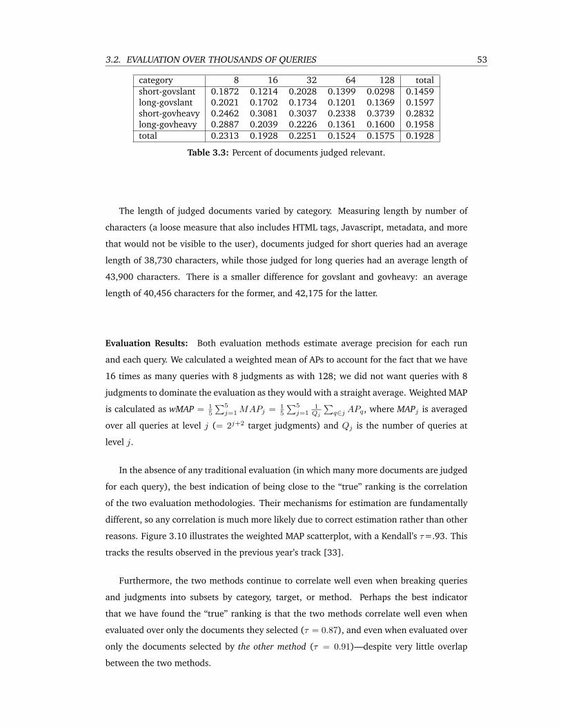
3.2. EVALUATION OVER THOUSANDS OF QUERIES 53
category 8 16 32 64 128 totalshort-govslant 0.1872 0.1214 0.2028 0.1399 0.0298 0.1459long-govslant 0.2021 0.1702 0.1734 0.1201 0.1369 0.1597short-govheavy 0.2462 0.3081 0.3037 0.2338 0.3739 0.2832long-govheavy 0.2887 0.2039 0.2226 0.1361 0.1600 0.1958total 0.2313 0.1928 0.2251 0.1524 0.1575 0.1928
Table 3.3: Percent of documents judged relevant.
The length of judged documents varied by category. Measuring length by number of
characters (a loose measure that also includes HTML tags, Javascript, metadata, and more
that would not be visible to the user), documents judged for short queries had an average
length of 38,730 characters, while those judged for long queries had an average length of
43,900 characters. There is a smaller difference for govslant and govheavy: an average
length of 40,456 characters for the former, and 42,175 for the latter.
Evaluation Results: Both evaluation methods estimate average precision for each run
and each query. We calculated a weighted mean of APs to account for the fact that we have
16 times as many queries with 8 judgments as with 128; we did not want queries with 8
judgments to dominate the evaluation as they would with a straight average. Weighted MAP
is calculated as wMAP = 15
∑5j=1 MAPj = 1
5
∑5j=1
1Qj
∑q∈j APq, where MAPj is averaged
over all queries at level j (= 2j+2 target judgments) and Qj is the number of queries at
level j.
In the absence of any traditional evaluation (in which many more documents are judged
for each query), the best indication of being close to the “true” ranking is the correlation
of the two evaluation methodologies. Their mechanisms for estimation are fundamentally
different, so any correlation is much more likely due to correct estimation rather than other
reasons. Figure 3.10 illustrates the weighted MAP scatterplot, with a Kendall’s τ=.93. This
tracks the results observed in the previous year’s track [33].
Furthermore, the two methods continue to correlate well even when breaking queries
and judgments into subsets by category, target, or method. Perhaps the best indicator
that we have found the “true” ranking is that the two methods correlate well even when
evaluated over only the documents they selected (τ = 0.87), and even when evaluated over
only the documents selected by the other method (τ = 0.91)—despite very little overlap
between the two methods.
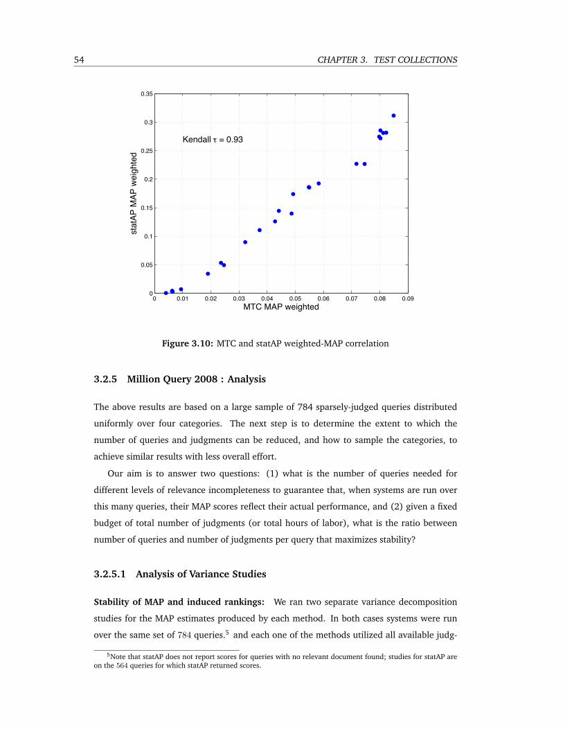
54 CHAPTER 3. TEST COLLECTIONS
0 0.01 0.02 0.03 0.04 0.05 0.06 0.07 0.08 0.090
0.05
0.1
0.15
0.2
0.25
0.3
0.35
MTC MAP weighted
stat
AP M
AP w
eigh
ted
Kendall ! = 0.93
Figure 3.10: MTC and statAP weighted-MAP correlation
3.2.5 Million Query 2008 : Analysis
The above results are based on a large sample of 784 sparsely-judged queries distributed
uniformly over four categories. The next step is to determine the extent to which the
number of queries and judgments can be reduced, and how to sample the categories, to
achieve similar results with less overall effort.
Our aim is to answer two questions: (1) what is the number of queries needed for
different levels of relevance incompleteness to guarantee that, when systems are run over
this many queries, their MAP scores reflect their actual performance, and (2) given a fixed
budget of total number of judgments (or total hours of labor), what is the ratio between
number of queries and number of judgments per query that maximizes stability?
3.2.5.1 Analysis of Variance Studies
Stability of MAP and induced rankings: We ran two separate variance decomposition
studies for the MAP estimates produced by each method. In both cases systems were run
over the same set of 784 queries.5 and each one of the methods utilized all available judg-
5Note that statAP does not report scores for queries with no relevant document found; studies for statAP areon the 564 queries for which statAP returned scores.
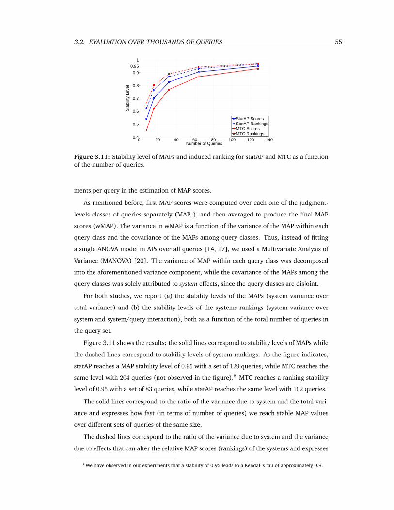
3.2. EVALUATION OVER THOUSANDS OF QUERIES 55
0 20 40 60 80 100 120 1400.4
0.5
0.6
0.7
0.8
0.9
0.95
1
Number of Queries
Sta
bilit
y Le
vel
StatAP ScoresStatAP RankingsMTC ScoresMTC Rankings
Figure 3.11: Stability level of MAPs and induced ranking for statAP and MTC as a functionof the number of queries.
ments per query in the estimation of MAP scores.
As mentioned before, first MAP scores were computed over each one of the judgment-
levels classes of queries separately (MAPc), and then averaged to produce the final MAP
scores (wMAP). The variance in wMAP is a function of the variance of the MAP within each
query class and the covariance of the MAPs among query classes. Thus, instead of fitting
a single ANOVA model in APs over all queries [14, 17], we used a Multivariate Analysis of
Variance (MANOVA) [20]. The variance of MAP within each query class was decomposed
into the aforementioned variance component, while the covariance of the MAPs among the
query classes was solely attributed to system effects, since the query classes are disjoint.
For both studies, we report (a) the stability levels of the MAPs (system variance over
total variance) and (b) the stability levels of the systems rankings (system variance over
system and system/query interaction), both as a function of the total number of queries in
the query set.
Figure 3.11 shows the results: the solid lines correspond to stability levels of MAPs while
the dashed lines correspond to stability levels of system rankings. As the figure indicates,
statAP reaches a MAP stability level of 0.95 with a set of 129 queries, while MTC reaches the
same level with 204 queries (not observed in the figure).6 MTC reaches a ranking stability
level of 0.95 with a set of 83 queries, while statAP reaches the same level with 102 queries.
The solid lines correspond to the ratio of the variance due to system and the total vari-
ance and expresses how fast (in terms of number of queries) we reach stable MAP values
over different sets of queries of the same size.
The dashed lines correspond to the ratio of the variance due to system and the variance
due to effects that can alter the relative MAP scores (rankings) of the systems and expresses
6We have observed in our experiments that a stability of 0.95 leads to a Kendall’s tau of approximately 0.9.
56 CHAPTER 3. TEST COLLECTIONS
0 20 40 60 80 100 120 1400.5
0.6
0.7
0.8
0.9
1MAP − 16 judgments (max) per query
Number of Queries
Sta
bilit
y Le
vel
StatAP ScoresStatAP RankingsMTC ScoresMTC Rankings
0 20 40 60 80 100 120 140
0.65
0.7
0.75
0.8
0.85
0.9
0.95
1MAP − 32 judgments (max) per query
Number of Queries
Sta
bilit
y Le
vel
StatAP ScoresStatAP RankingsMTC ScoresMTC Rankings
0 20 40 60 80 100 120 140
0.65
0.7
0.75
0.8
0.85
0.9
0.95
1MAP − 64 judgments (max) per query
Number of Queries
Sta
bilit
y Le
vel
StatAP ScoresStatAP RankingsMTC ScoresMTC Rankings
0 20 40 60 80 100 120 1400.5
0.55
0.6
0.65
0.7
0.75
0.8
0.85
0.9
0.95
1MAP − 128 judgments (max) per query
Number of Queries
Sta
bilit
y Le
vel
StatAP ScoresStatAP RankingsMTC ScoresMTC Rankings
Figure 3.12: Stability levels of MAP scores and induced ranking for statAP and MTC as afunction of the number of queries for different levels of relevance incompleteness.
how fast (in terms of number of queries) we reach stable system rankings.
Note that the queries in the query set are distributed in the same manner as in the
original data, i.e. the number of queries in each class is inversely proportional to the level
of relevance incompleteness.
These results again support the claims that the statAP method, by design, aims to esti-
mate the actual MAP scores of the systems, while the MTC method, by design, aims to infer
the proper ranking of systems.
Stability with incomplete judgments: To illustrate how stable the MAPs returned by
the two methods are with respect to different levels of relevance incompleteness, we ran
ANOVA studies for the each one of the query classes separately. Figure 3.12 demonstrate
the stability levels for both methods when 16, 32, 64, and 128 judgments are available,
respectively.
According to stability levels illustrated in these figures, MTC leads to both more stable
MAPs and induced rankings than statAP when 16 or 32 relevance judgments are available
per query, while the opposite is true when 64 or 128 relevance judgments are available.
Note that the stability of the MAP scores returned by statAP degrades with the relevance
incompleteness, as expected. On the other hand, the opposite is true for MTC. For the
estimation of MAP scores, MTC is employing a prior distribution of relevance which is cal-
culated by combining information from all queries, which violates the query independence
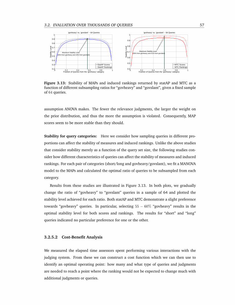
3.2. EVALUATION OVER THOUSANDS OF QUERIES 57
0 0.2 0.4 0.6 0.8 10.2
0.3
0.4
0.5
0.6
0.7
0.8
0.9
1
Fraction of Queries from the ’govheavy’ category
Sta
bilit
y Le
vel
’govheavy’ vs. ’govslant’ − 64 Queries
StatAP ScoresStatAP Rankings
Maximum Stability Level(56% from govheavy and 44% from govslant)
0 0.2 0.4 0.6 0.8 10.4
0.5
0.6
0.7
0.8
0.9
1’govheavy’ vs. ’govslant’ − 64 Queries
Fraction of Queries from the ’govheavy’ category
Sta
bilit
y Le
vel
MTC ScoresMTC Rankings
Maximum Stability Level(59% from govheavy and 41% from govslant)
Figure 3.13: Stability of MAPs and induced rankings returned by statAP and MTC as afunction of different subsampling ratios for “govheavy” and “govslant”, given a fixed sampleof 64 queries.
assumption ANOVA makes. The fewer the relevance judgments, the larger the weight on
the prior distribution, and thus the more the assumption is violated. Consequently, MAP
scores seem to be more stable than they should.
Stability for query categories: Here we consider how sampling queries in different pro-
portions can affect the stability of measures and induced rankings. Unlike the above studies
that consider stability merely as a function of the query set size, the following studies con-
sider how different characteristics of queries can affect the stability of measures and induced
rankings. For each pair of categories (short/long and govheavy/govslant), we fit a MANOVA
model to the MAPs and calculated the optimal ratio of queries to be subsampled from each
category.
Results from these studies are illustrated in Figure 3.13. In both plots, we gradually
change the ratio of “govheavy” to “govslant” queries in a sample of 64 and plotted the
stability level achieved for each ratio. Both statAP and MTC demonstrate a slight preference
towards “govheavy” queries. In particular, selecting 55 − 60% “govheavy” results in the
optimal stability level for both scores and rankings. The results for “short” and “long”
queries indicated no particular preference for one or the other.
3.2.5.2 Cost-Benefit Analysis
We measured the elapsed time assessors spent performing various interactions with the
judging system. From these we can construct a cost function which we can then use to
identify an optimal operating point: how many and what type of queries and judgments
are needed to reach a point where the ranking would not be expected to change much with
additional judgments or queries.
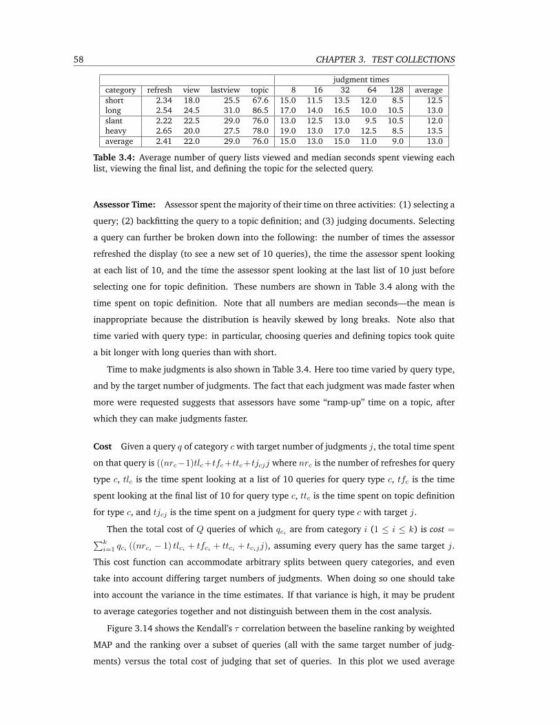
58 CHAPTER 3. TEST COLLECTIONS
judgment timescategory refresh view lastview topic 8 16 32 64 128 averageshort 2.34 18.0 25.5 67.6 15.0 11.5 13.5 12.0 8.5 12.5long 2.54 24.5 31.0 86.5 17.0 14.0 16.5 10.0 10.5 13.0slant 2.22 22.5 29.0 76.0 13.0 12.5 13.0 9.5 10.5 12.0heavy 2.65 20.0 27.5 78.0 19.0 13.0 17.0 12.5 8.5 13.5average 2.41 22.0 29.0 76.0 15.0 13.0 15.0 11.0 9.0 13.0
Table 3.4: Average number of query lists viewed and median seconds spent viewing eachlist, viewing the final list, and defining the topic for the selected query.
Assessor Time: Assessor spent the majority of their time on three activities: (1) selecting a
query; (2) backfitting the query to a topic definition; and (3) judging documents. Selecting
a query can further be broken down into the following: the number of times the assessor
refreshed the display (to see a new set of 10 queries), the time the assessor spent looking
at each list of 10, and the time the assessor spent looking at the last list of 10 just before
selecting one for topic definition. These numbers are shown in Table 3.4 along with the
time spent on topic definition. Note that all numbers are median seconds—the mean is
inappropriate because the distribution is heavily skewed by long breaks. Note also that
time varied with query type: in particular, choosing queries and defining topics took quite
a bit longer with long queries than with short.
Time to make judgments is also shown in Table 3.4. Here too time varied by query type,
and by the target number of judgments. The fact that each judgment was made faster when
more were requested suggests that assessors have some “ramp-up” time on a topic, after
which they can make judgments faster.
Cost Given a query q of category c with target number of judgments j, the total time spent
on that query is ((nrc−1)tlc+tfc+ttc+tjcjj where nrc is the number of refreshes for query
type c, tlc is the time spent looking at a list of 10 queries for query type c, tfc is the time
spent looking at the final list of 10 for query type c, ttc is the time spent on topic definition
for type c, and tjcj is the time spent on a judgment for query type c with target j.
Then the total cost of Q queries of which qci are from category i (1 ≤ i ≤ k) is cost =∑ki=1 qci
((nrci− 1) tlci
+ tfci+ ttci
+ tcijj), assuming every query has the same target j.
This cost function can accommodate arbitrary splits between query categories, and even
take into account differing target numbers of judgments. When doing so one should take
into account the variance in the time estimates. If that variance is high, it may be prudent
to average categories together and not distinguish between them in the cost analysis.
Figure 3.14 shows the Kendall’s τ correlation between the baseline ranking by weighted
MAP and the ranking over a subset of queries (all with the same target number of judg-
ments) versus the total cost of judging that set of queries. In this plot we used average
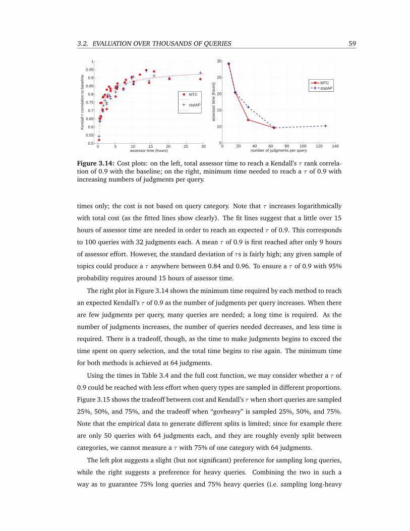
3.2. EVALUATION OVER THOUSANDS OF QUERIES 59
0 5 10 15 20 25 300.5
0.55
0.6
0.65
0.7
0.75
0.8
0.85
0.9
0.95
1
assessor time (hours)
Ken
dall
τ co
rrel
atio
n to
bas
elin
e
MTC
statAP
0 20 40 60 80 100 120 1405
10
15
20
25
30
number of judgments per query
asse
ssor
tim
e (h
ours
)
MTCstatAP
Figure 3.14: Cost plots: on the left, total assessor time to reach a Kendall’s τ rank correla-tion of 0.9 with the baseline; on the right, minimum time needed to reach a τ of 0.9 withincreasing numbers of judgments per query.
times only; the cost is not based on query category. Note that τ increases logarithmically
with total cost (as the fitted lines show clearly). The fit lines suggest that a little over 15
hours of assessor time are needed in order to reach an expected τ of 0.9. This corresponds
to 100 queries with 32 judgments each. A mean τ of 0.9 is first reached after only 9 hours
of assessor effort. However, the standard deviation of τs is fairly high; any given sample of
topics could produce a τ anywhere between 0.84 and 0.96. To ensure a τ of 0.9 with 95%
probability requires around 15 hours of assessor time.
The right plot in Figure 3.14 shows the minimum time required by each method to reach
an expected Kendall’s τ of 0.9 as the number of judgments per query increases. When there
are few judgments per query, many queries are needed; a long time is required. As the
number of judgments increases, the number of queries needed decreases, and less time is
required. There is a tradeoff, though, as the time to make judgments begins to exceed the
time spent on query selection, and the total time begins to rise again. The minimum time
for both methods is achieved at 64 judgments.
Using the times in Table 3.4 and the full cost function, we may consider whether a τ of
0.9 could be reached with less effort when query types are sampled in different proportions.
Figure 3.15 shows the tradeoff between cost and Kendall’s τ when short queries are sampled
25%, 50%, and 75%, and the tradeoff when “govheavy” is sampled 25%, 50%, and 75%.
Note that the empirical data to generate different splits is limited; since for example there
are only 50 queries with 64 judgments each, and they are roughly evenly split between
categories, we cannot measure a τ with 75% of one category with 64 judgments.
The left plot suggests a slight (but not significant) preference for sampling long queries,
while the right suggests a preference for heavy queries. Combining the two in such a
way as to guarantee 75% long queries and 75% heavy queries (i.e. sampling long-heavy
60 CHAPTER 3. TEST COLLECTIONS
0 2 4 6 8 10 12 14 16
0.6
0.65
0.7
0.75
0.8
0.85
0.9
assessor time (hours)
Ken
dall
τ co
rrel
atio
n to
bas
elin
e
25% short
50% short
75% short
0 2 4 6 8 10 12 14 16
0.6
0.65
0.7
0.75
0.8
0.85
0.9
assessor time (hours)
Ken
dall
τ co
rrel
atio
n to
bas
elin
e
25% heavy
50% heavy
75% heavy
Figure 3.15: Cost plots. On the left, sampling short versus long in different proportions.On the right, sampling heavy versus slant in different proportions.
0.75 × 0.75 = 0.56, long-slant 0.19, short-heavy 0.19, and short-slant 0.06), an expected
Kendall’s τ of 0.9 is reached after a little over 4 hours of assessor effort.
3.2.6 Conclusion
We put in practice two recently developed evaluation techniques that, unlike standard eval-
uation, scale easily and allow many more experiments and analyses. We experimented with
24 submitted systems and 10,000 queries evaluating 1,692 of them with about 70,000 judg-
ments in 2007 and with 25 submitted systems over 10000 queries, evaluating 784 of them
with only about 15000 judgments in 2008.
Evaluation stability. The setup allowed an analysis of evaluation stability with fewer
judgments or queries. Using ANOVA, we concluded that MTC needs about 50-100 queries
with approximately 2000 total judgments for a reliable ranking, while statAP needs about
130-150 queries with approximately 2800 total judgments for a reliable estimate of MAP.
Many queries; categories. In 2008, we investigated system performance over pre-
assigned query categories. There is some evidence that over-sampling some types of queries
may result in cheaper (if not substantially more efficient) evaluation: over-sampling long
and govheavy queries resulted in a good ranking with just a little over four hours of sim-
ulated assessor time. More investigation to find the right tradeoffs is a clear direction for
future work.
Cost analysis; optimal budget. Finally, in 2008, queries were randomly assigned 5
different target numbers of judgments such that the total number of judgments for each
class is roughly constant. This split facilitated a derivation of optimal budgeting for IR
evaluation via cost (in assessor hours) analysis. We concluded that 30-60 judgments per
query with around 100 queries is optimal for assessing systems’ performance ranking.

3.3. OVERALL CONCLUSIONS 61
3.3 Overall Conclusions
The size of test collections used in IR evaluation has been growing at a tremendous pace.
While collection sizes keep increases, the budget for relevance judgments does not. Reliable
evaluations will rely more and more on the relevance judgments being selected intelligently
and the inferences about systems made robustly despite many missing judgments. In this
chapter we first proposed a low-cost evaluation methodology based on stratified sampling
to intelligently select only a subset of documents per query to be judged. Our experiments
demonstrated that one can reliably evaluate retrieval systems with about 5% of the total
judgments that would be required if the traditional depth-pooling method was employed.
Then, by utilizing document selection methodologies similar to our proposed one we con-
cluded that given a fixed budget evaluating systems over many queries with few judgments
per query leads to more reliable and thus more efficient evaluation than evaluating systems
over few queries with larger number of judgments per query. Finally, we demonstrated that
some query categories can indeed be more useful in evaluation than others. For instance
oversampling long queries with many user clicks (which, to some extent, designate that the
query is appropriate for the subset of searchable material that constitute the collection) can
lead to more reliable and thus more efficient evaluation.


CHAPTER 4
Training Collections
Ranking is a central problem in information retrieval. Modern search engines, especially
those designed for the World Wide Web, commonly analyze and combine hundreds of fea-
tures extracted from the submitted query and underlying documents in order to assess the
relative relevance of a document to a given query and thus rank the underlying collection.
The sheer size of this problem has led to the development of learning-to-rank algorithms
that can automate the construction of such ranking functions: Given a training set of (fea-
ture vector, relevance) pairs, a machine learning procedure learns how to combine the
query and document features in such a way so as to effectively assess the relevance of any
document to any query and thus rank a collection in response to a user input.
Given that document corpora have been increasing in size it is practically infeasible (1)
to extract features from all document-query pairs, (2) to judge each document as relevant
or irrelevant to each query, and (3) to train learning-to-rank algorithms over such a vast
data set.
Even though extracting features and training ranking algorithms is computationally ex-
pensive, annotating documents with relevance grades is the main bottleneck in constructing
training collection, since human effort is required. It is essential therefore, both for the ef-
ficiency of the construction methodology and for the efficiency of the training algorithm,
that only a small subset of documents be selected. The document selection, though, should
be done in a way that does not harm the effectiveness of learning.
Unlike document selection for learning-to-rank, where little work has been done, a sig-
nificant volume of work has appeared in the literature regarding document selection for
efficient and effective evaluation of retrieval systems [5, 32, 33, 146, 148, 110], including
the methodology presented in Section 3.1. Here, we explore the duality between document
selection methodologies for evaluation and document selection methodologies for learning-
to-rank. The main question we ask is : “Can any of the methodologies designed for efficient
evaluation also be used for constructing effective learning collections? If yes, which one of
these methods is better for this purpose?”
63
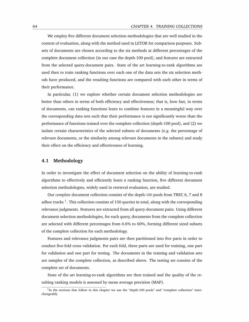
64 CHAPTER 4. TRAINING COLLECTIONS
We employ five different document selection methodologies that are well studied in the
context of evaluation, along with the method used in LETOR for comparison purposes. Sub-
sets of documents are chosen according to the six methods at different percentages of the
complete document collection (in our case the depth-100 pool), and features are extracted
from the selected query-document pairs. State of the art learning-to-rank algorithms are
used then to train ranking functions over each one of the data sets the six selection meth-
ods have produced, and the resulting functions are compared with each other in terms of
their performance.
In particular, (1) we explore whether certain document selection methodologies are
better than others in terms of both efficiency and effectiveness; that is, how fast, in terms
of documents, can ranking functions learn to combine features in a meaningful way over
the corresponding data sets such that their performance is not significantly worse than the
performance of functions trained over the complete collection (depth-100 pool), and (2) we
isolate certain characteristics of the selected subsets of documents (e.g. the percentage of
relevant documents, or the similarity among relevant documents in the subsets) and study
their effect on the efficiency and effectiveness of learning.
4.1 Methodology
In order to investigate the effect of document selection on the ability of learning-to-rank
algorithms to effectively and efficiently learn a ranking function, five different document
selection methodologies, widely used in retrieval evaluation, are studied.
Our complete document collection consists of the depth-100 pools from TREC 6, 7 and 8
adhoc tracks 1. This collection consists of 150 queries in total, along with the corresponding
relevance judgments. Features are extracted from all query-document pairs. Using different
document selection methodologies, for each query, documents from the complete collection
are selected with different percentages from 0.6% to 60%, forming different sized subsets
of the complete collection for each methodology.
Features and relevance judgments pairs are then partitioned into five parts in order to
conduct five-fold cross validation. For each fold, three parts are used for training, one part
for validation and one part for testing. The documents in the training and validation sets
are samples of the complete collection, as described above. The testing set consists of the
complete set of documents.
State of the art learning-to-rank algorithms are then trained and the quality of the re-
sulting ranking models is assessed by mean average precision (MAP).
1In the sections that follow in this chapter we use the “depth-100 pools” and “complete collection” inter-changeably

4.1. METHODOLOGY 65
4.1.1 Data sets
The document corpus, the queries and the relevance judgments are obtained from TREC 6,
7 and 8 ad-hoc retrieval track.
The document corpus consists of approximately half a million documents (528,155)
from the Financial Times, the Federal Register, the Foreign Broadcast Information Service
and the LA Times document collections [134].
The queries were developed by NIST assessors and they were chosen based on their
estimated number of relevant documents in the corpus. Collectively, 150 such queries were
developed. A number of retrieval systems were run over these queries and for each query
the depth-100 pools of the returned documents were judged as relevant or irrelevant by the
same NIST assessor that issued the query.
We extract features from all query-document pairs. The features extracted are shown in
Table 4.1.1 and they are a subset of the LETOR3.0 features [128].
For the computation of the IDF (inverse document frequency) of a query term qi, as in
LETOR3.0, we adopted the widely used formula,
idf(qi) = logN − n(qi) + 0.5
n(qi) + 0.5
where n(qi) is the number of documents containing qi and N is the total number of docu-
ments in the collection. Since a query may contains more than one term, the final value of
IDF is the sum of the IDF of each query term:
idf(Q) =∑qi
idf(qi)
Note that IDF is document independent, and so all the documents under a query have same
IDF values.
The BM25 score of a document D for a query Q, containing the terms q1, q2, ..., qn is
computed as:
BM25(D,Q) =∑
i:f(qi,D)>0
idf(qi) ·f(qi, D) · (k1 + 1)
f(qi, D) + k1 · (1− b + b · |D|avgdl )
· (k3 + 1)f(qi, Q)k3 + f(qi;Q)
where idf(qi) is defined as above, f(qi, D) is the occurrences of qi in the document D,
f(qi, Q) is the occurrences of qi in the query Q, |D| is the length of the document D (i.e.,
the number of words), and avgdl is the average document length in the entire document
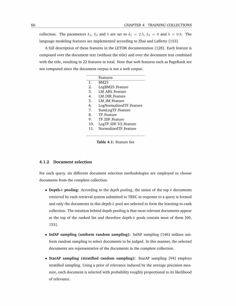
66 CHAPTER 4. TRAINING COLLECTIONS
collection. The parameters k1, k3 and b are set to k1 = 2.5, k3 = 0 and b = 0.8. The
language modeling features are implemented according to Zhai and Lafferty [153].
A full description of these features in the LETOR documentation [128]. Each feature is
computed over the document text (without the title) and over the document text combined
with the title, resulting in 22 features in total. Note that web features such as PageRank are
not computed since the document corpus is not a web corpus.
Features1. BM252. LogBM25 Feature3. LM ABS Feature4. LM DIR Feature5. LM JM Feature6. LogNormalizedTF Feature7. SumLogTF Feature8. TF Feature9. TF IDF Feature10. LogTF IDF V2 Feature11. NormalizedTF Feature
Table 4.1: Feature Set
4.1.2 Document selection
For each query, six different document selection methodologies are employed to choose
documents from the complete collection:
• Depth-k pooling: According to the depth pooling, the union of the top k documents
retrieved by each retrieval system submitted to TREC in response to a query is formed
and only the documents in this depth-k pool are selected to form the learning-to-rank
collection. The intuition behind depth-pooling is that most relevant documents appear
at the top of the ranked list and therefore depth-k pools contain most of them [60,
155].
• InfAP sampling (uniform random sampling): InfAP sampling [146] utilizes uni-
form random sampling to select documents to be judged. In this manner, the selected
documents are representative of the documents in the complete collection.
• StatAP sampling (stratified random sampling): StatAP sampling [94] employs
stratified sampling. Using a prior of relevance induced by the average precision mea-
sure, each document is selected with probability roughly proportional to its likelihood
of relevance.
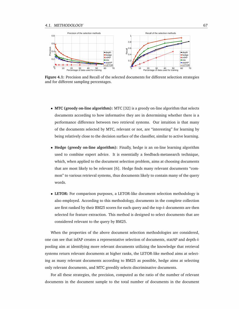
4.1. METHODOLOGY 67
0 10 20 30 40 50 60 700
0.2
0.4
0.6
0.8
Percentage of data used for training
Pre
cisi
on
Precision of the selection methods
depthhedgeinfAPmtcstatAPLETOR
0 10 20 30 40 50 60 700
0.2
0.4
0.6
0.8
1
Percentage of data used for training
Rec
all
Recall of the selection methods
depthhedgeinfAPmtcstatAPLETOR
Figure 4.1: Precision and Recall of the selected documents for different selection strategiesand for different sampling percentages.
• MTC (greedy on-line algorithm): MTC [32] is a greedy on-line algorithm that selects
documents according to how informative they are in determining whether there is a
performance difference between two retrieval systems. Our intuition is that many
of the documents selected by MTC, relevant or not, are “interesting” for learning by
being relatively close to the decision surface of the classifier, similar to active learning.
• Hedge (greedy on-line algorithm): Finally, hedge is an on-line learning algorithm
used to combine expert advice. It is essentially a feedback-metasearch technique,
which, when applied to the document selection problem, aims at choosing documents
that are most likely to be relevant [6]. Hedge finds many relevant documents “com-
mon” to various retrieval systems, thus documents likely to contain many of the query
words.
• LETOR: For comparison purposes, a LETOR-like document selection methodology is
also employed. According to this methodology, documents in the complete collection
are first ranked by their BM25 scores for each query and the top-k documents are then
selected for feature extraction. This method is designed to select documents that are
considered relevant to the query by BM25.
When the properties of the above document selection methodologies are considered,
one can see that infAP creates a representative selection of documents, statAP and depth-k
pooling aim at identifying more relevant documents utilizing the knowledge that retrieval
systems return relevant documents at higher ranks, the LETOR-like method aims at select-
ing as many relevant documents according to BM25 as possible, hedge aims at selecting
only relevant documents, and MTC greedily selects discriminative documents.
For all these strategies, the precision, computed as the ratio of the number of relevant
documents in the document sample to the total number of documents in the document
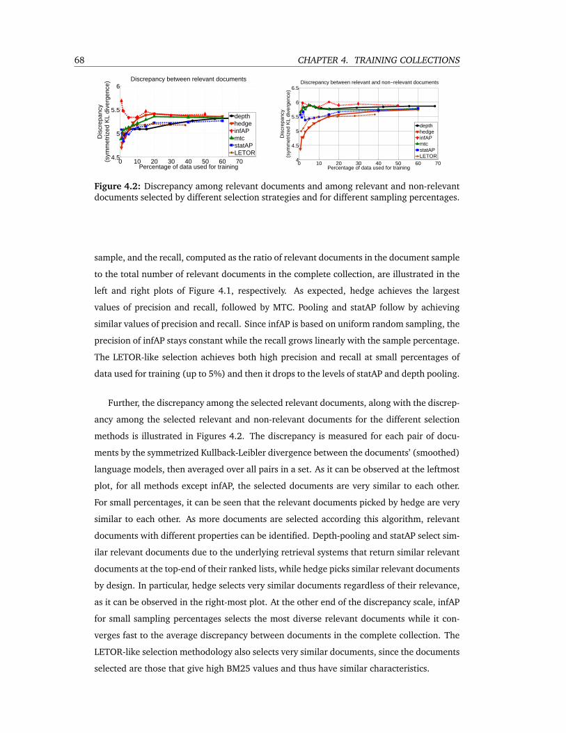
68 CHAPTER 4. TRAINING COLLECTIONS
0 10 20 30 40 50 60 704.5
5
5.5
6
Percentage of data used for training
Dis
crep
ancy
(sym
met
rized
KL
dive
rgen
ce) Discrepancy between relevant documents
depthhedgeinfAPmtcstatAPLETOR
0 10 20 30 40 50 60 704
4.5
5
5.5
6
6.5
Percentage of data used for training
Dis
crep
ancy
(sym
met
rized
KL
dive
rgen
ce)
Discrepancy between relevant and non−relevant documents
depthhedgeinfAPmtcstatAPLETOR
Figure 4.2: Discrepancy among relevant documents and among relevant and non-relevantdocuments selected by different selection strategies and for different sampling percentages.
sample, and the recall, computed as the ratio of relevant documents in the document sample
to the total number of relevant documents in the complete collection, are illustrated in the
left and right plots of Figure 4.1, respectively. As expected, hedge achieves the largest
values of precision and recall, followed by MTC. Pooling and statAP follow by achieving
similar values of precision and recall. Since infAP is based on uniform random sampling, the
precision of infAP stays constant while the recall grows linearly with the sample percentage.
The LETOR-like selection achieves both high precision and recall at small percentages of
data used for training (up to 5%) and then it drops to the levels of statAP and depth pooling.
Further, the discrepancy among the selected relevant documents, along with the discrep-
ancy among the selected relevant and non-relevant documents for the different selection
methods is illustrated in Figures 4.2. The discrepancy is measured for each pair of docu-
ments by the symmetrized Kullback-Leibler divergence between the documents’ (smoothed)
language models, then averaged over all pairs in a set. As it can be observed at the leftmost
plot, for all methods except infAP, the selected documents are very similar to each other.
For small percentages, it can be seen that the relevant documents picked by hedge are very
similar to each other. As more documents are selected according this algorithm, relevant
documents with different properties can be identified. Depth-pooling and statAP select sim-
ilar relevant documents due to the underlying retrieval systems that return similar relevant
documents at the top-end of their ranked lists, while hedge picks similar relevant documents
by design. In particular, hedge selects very similar documents regardless of their relevance,
as it can be observed in the right-most plot. At the other end of the discrepancy scale, infAP
for small sampling percentages selects the most diverse relevant documents while it con-
verges fast to the average discrepancy between documents in the complete collection. The
LETOR-like selection methodology also selects very similar documents, since the documents
selected are those that give high BM25 values and thus have similar characteristics.
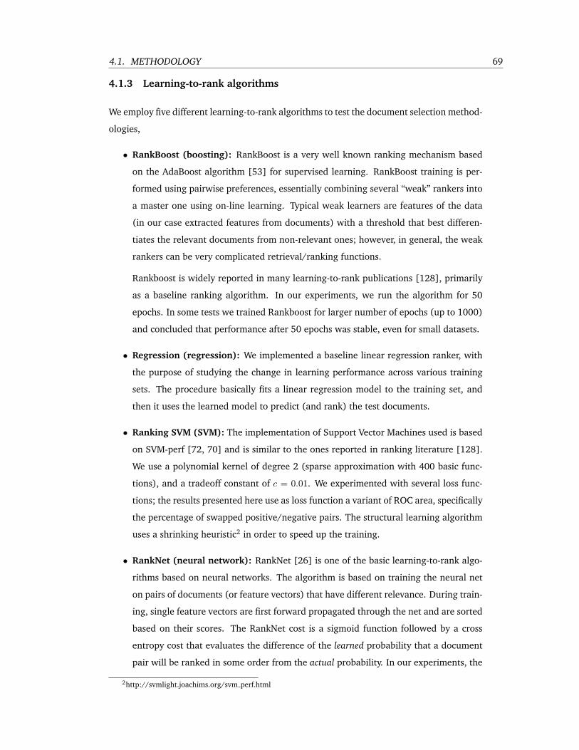
4.1. METHODOLOGY 69
4.1.3 Learning-to-rank algorithms
We employ five different learning-to-rank algorithms to test the document selection method-
ologies,
• RankBoost (boosting): RankBoost is a very well known ranking mechanism based
on the AdaBoost algorithm [53] for supervised learning. RankBoost training is per-
formed using pairwise preferences, essentially combining several “weak” rankers into
a master one using on-line learning. Typical weak learners are features of the data
(in our case extracted features from documents) with a threshold that best differen-
tiates the relevant documents from non-relevant ones; however, in general, the weak
rankers can be very complicated retrieval/ranking functions.
Rankboost is widely reported in many learning-to-rank publications [128], primarily
as a baseline ranking algorithm. In our experiments, we run the algorithm for 50
epochs. In some tests we trained Rankboost for larger number of epochs (up to 1000)
and concluded that performance after 50 epochs was stable, even for small datasets.
• Regression (regression): We implemented a baseline linear regression ranker, with
the purpose of studying the change in learning performance across various training
sets. The procedure basically fits a linear regression model to the training set, and
then it uses the learned model to predict (and rank) the test documents.
• Ranking SVM (SVM): The implementation of Support Vector Machines used is based
on SVM-perf [72, 70] and is similar to the ones reported in ranking literature [128].
We use a polynomial kernel of degree 2 (sparse approximation with 400 basic func-
tions), and a tradeoff constant of c = 0.01. We experimented with several loss func-
tions; the results presented here use as loss function a variant of ROC area, specifically
the percentage of swapped positive/negative pairs. The structural learning algorithm
uses a shrinking heuristic2 in order to speed up the training.
• RankNet (neural network): RankNet [26] is one of the basic learning-to-rank algo-
rithms based on neural networks. The algorithm is based on training the neural net
on pairs of documents (or feature vectors) that have different relevance. During train-
ing, single feature vectors are first forward propagated through the net and are sorted
based on their scores. The RankNet cost is a sigmoid function followed by a cross
entropy cost that evaluates the difference of the learned probability that a document
pair will be ranked in some order from the actual probability. In our experiments, the
2http://svmlight.joachims.org/svm perf.html
70 CHAPTER 4. TRAINING COLLECTIONS
training was run for 300 epochs (no significant improvement was observed if more
epochs were used).
• LambdaRank (neural network): LambdaRank [27] aims at directly optimizing an
IR metric, in particular, NDCG. Since the IR metrics are not smooth as they depends
on ranks of documents, it uses the approach of defining the gradient of the target
evaluation metric only at the points needed. Given a pair of documents, the gradients
used in LambdaRank are obtained by scaling the RankNet cost with the amount of
change in the value of the metric obtained by swapping the two documents. Similar
to RankNet, LambdaRank training was also run for 300 epochs.
As a summary, RankBoost optimizes for pairwise preferences, Regression optimizes for
classification error in the relevance judgments, and SVM optimizes for the area under the
ROC curve. RankNet aims to optimize for the probability that two documents are ranked
in correct order in the ranking. Finally, LambdaRank directly optimizes for nDCG and even
though the gradients are virtually defined, the method is shown to find the local optimum
for the target metric.
All the algorithms, with the exception of Regression, are “pair-wise” because they con-
sider pairs of documents while training, either directly in the learning mechanism or indi-
rectly in the loss function.
4.2 Results
The performance of the learning-to-rank algorithms when trained over the different data
sets produced by the six document selection methodologies is illustrated in Figure 4.3. The
x-axis on the plots is the percentage of documents sampled from the complete document
collection (depth-100 pool). The performance of the rankers (y-axis) is measured by the
mean average precision (MAP) of the ranked list of documents returned by the rankers in
response to the queries in the testing data sets. Each one of the document selection methods
employed corresponds to a curve in the plot.
As one can observe in Figure 4.3, for most of the cases, the learning-to-rank algorithms
reach almost optimal performance with as little training data as 1% of the complete collec-
tion. The Student’s t statistical test was employed in order to test whether the difference
among the achieved MAP scores of the ranking function for different sampling percent-
ages and the maximum MAP score the ranking functions obtain (MAP using full training
data) are statistically significant. The t-test exhibits no significant differences for ranking
functions trained over infAP, statAP, depth-pooling and MTC at any of document sampling
percentage above 2%.
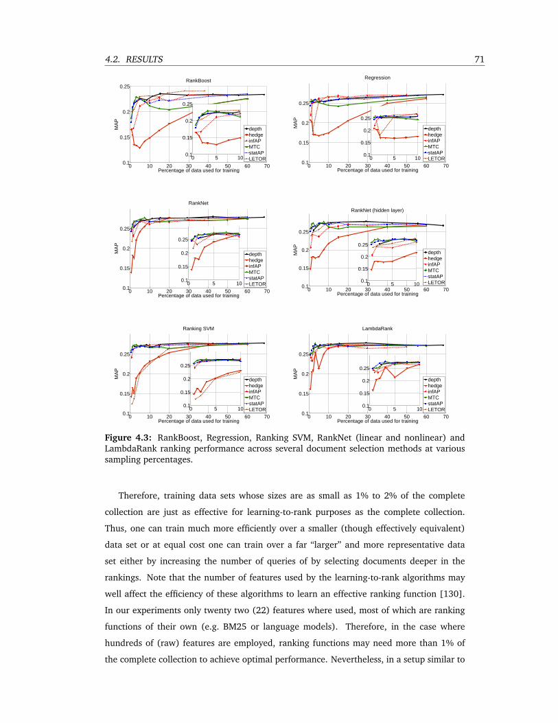
4.2. RESULTS 71
0 10 20 30 40 50 60 700.1
0.15
0.2
0.25
Percentage of data used for training
MA
P
RankBoost
depthhedgeinfAPMTCstatAPLETOR0 5 10
0.1
0.15
0.2
0.25
0 10 20 30 40 50 60 700.1
0.15
0.2
0.25
Percentage of data used for training
MA
P
Regression
depthhedgeinfAPMTCstatAPLETOR0 5 10
0.1
0.15
0.2
0.25
0 10 20 30 40 50 60 700.1
0.15
0.2
0.25
Percentage of data used for training
MA
P
RankNet
depthhedgeinfAPMTCstatAPLETOR0 5 10
0.1
0.15
0.2
0.25
0 10 20 30 40 50 60 700.1
0.15
0.2
0.25
Percentage of data used for trainingM
AP
RankNet (hidden layer)
depthhedgeinfAPMTCstatAPLETOR0 5 10
0.1
0.15
0.2
0.25
0 10 20 30 40 50 60 700.1
0.15
0.2
0.25
Percentage of data used for training
MA
P
Ranking SVM
depthhedgeinfAPMTCstatAPLETOR0 5 10
0.1
0.15
0.2
0.25
0 10 20 30 40 50 60 700.1
0.15
0.2
0.25
Percentage of data used for training
MA
P
LambdaRank
depthhedgeinfAPMTCstatAPLETOR0 5 10
0.1
0.15
0.2
0.25
Figure 4.3: RankBoost, Regression, Ranking SVM, RankNet (linear and nonlinear) andLambdaRank ranking performance across several document selection methods at varioussampling percentages.
Therefore, training data sets whose sizes are as small as 1% to 2% of the complete
collection are just as effective for learning-to-rank purposes as the complete collection.
Thus, one can train much more efficiently over a smaller (though effectively equivalent)
data set or at equal cost one can train over a far “larger” and more representative data
set either by increasing the number of queries of by selecting documents deeper in the
rankings. Note that the number of features used by the learning-to-rank algorithms may
well affect the efficiency of these algorithms to learn an effective ranking function [130].
In our experiments only twenty two (22) features where used, most of which are ranking
functions of their own (e.g. BM25 or language models). Therefore, in the case where
hundreds of (raw) features are employed, ranking functions may need more than 1% of
the complete collection to achieve optimal performance. Nevertheless, in a setup similar to
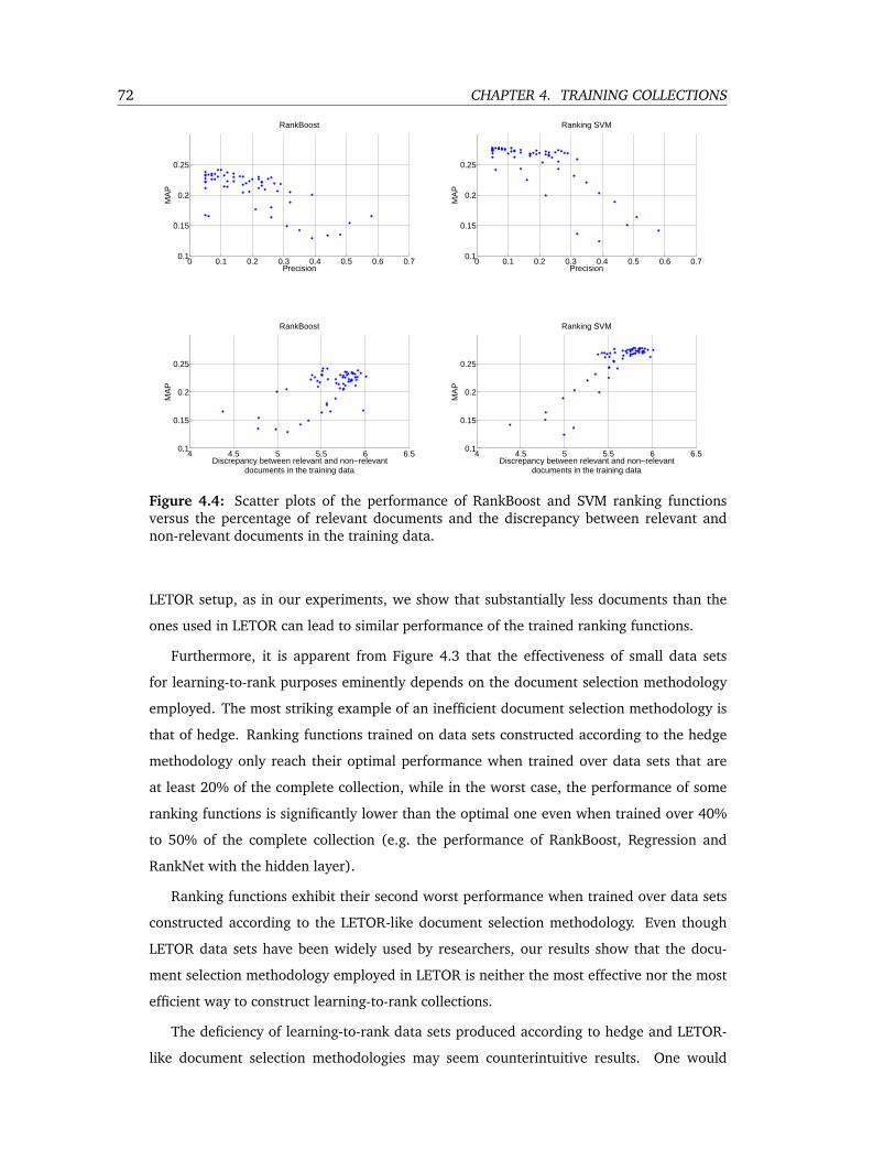
72 CHAPTER 4. TRAINING COLLECTIONS
0 0.1 0.2 0.3 0.4 0.5 0.6 0.70.1
0.15
0.2
0.25M
AP
Precision
RankBoost
0 0.1 0.2 0.3 0.4 0.5 0.6 0.70.1
0.15
0.2
0.25
MA
P
Precision
Ranking SVM
4 4.5 5 5.5 6 6.50.1
0.15
0.2
0.25
MA
P
Discrepancy between relevant and non−relevantdocuments in the training data
RankBoost
4 4.5 5 5.5 6 6.50.1
0.15
0.2
0.25
MA
PDiscrepancy between relevant and non−relevant
documents in the training data
Ranking SVM
Figure 4.4: Scatter plots of the performance of RankBoost and SVM ranking functionsversus the percentage of relevant documents and the discrepancy between relevant andnon-relevant documents in the training data.
LETOR setup, as in our experiments, we show that substantially less documents than the
ones used in LETOR can lead to similar performance of the trained ranking functions.
Furthermore, it is apparent from Figure 4.3 that the effectiveness of small data sets
for learning-to-rank purposes eminently depends on the document selection methodology
employed. The most striking example of an inefficient document selection methodology is
that of hedge. Ranking functions trained on data sets constructed according to the hedge
methodology only reach their optimal performance when trained over data sets that are
at least 20% of the complete collection, while in the worst case, the performance of some
ranking functions is significantly lower than the optimal one even when trained over 40%
to 50% of the complete collection (e.g. the performance of RankBoost, Regression and
RankNet with the hidden layer).
Ranking functions exhibit their second worst performance when trained over data sets
constructed according to the LETOR-like document selection methodology. Even though
LETOR data sets have been widely used by researchers, our results show that the docu-
ment selection methodology employed in LETOR is neither the most effective nor the most
efficient way to construct learning-to-rank collections.
The deficiency of learning-to-rank data sets produced according to hedge and LETOR-
like document selection methodologies may seem counterintuitive results. One would
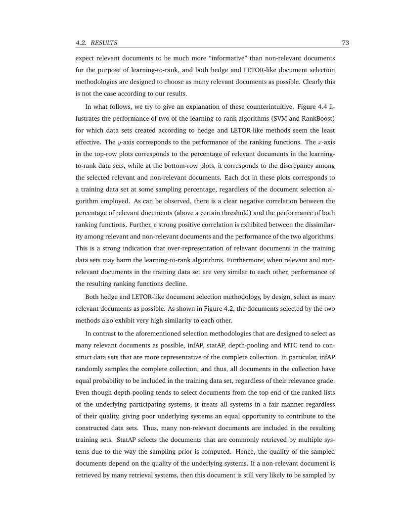
4.2. RESULTS 73
expect relevant documents to be much more “informative” than non-relevant documents
for the purpose of learning-to-rank, and both hedge and LETOR-like document selection
methodologies are designed to choose as many relevant documents as possible. Clearly this
is not the case according to our results.
In what follows, we try to give an explanation of these counterintuitive. Figure 4.4 il-
lustrates the performance of two of the learning-to-rank algorithms (SVM and RankBoost)
for which data sets created according to hedge and LETOR-like methods seem the least
effective. The y-axis corresponds to the performance of the ranking functions. The x-axis
in the top-row plots corresponds to the percentage of relevant documents in the learning-
to-rank data sets, while at the bottom-row plots, it corresponds to the discrepancy among
the selected relevant and non-relevant documents. Each dot in these plots corresponds to
a training data set at some sampling percentage, regardless of the document selection al-
gorithm employed. As can be observed, there is a clear negative correlation between the
percentage of relevant documents (above a certain threshold) and the performance of both
ranking functions. Further, a strong positive correlation is exhibited between the dissimilar-
ity among relevant and non-relevant documents and the performance of the two algorithms.
This is a strong indication that over-representation of relevant documents in the training
data sets may harm the learning-to-rank algorithms. Furthermore, when relevant and non-
relevant documents in the training data set are very similar to each other, performance of
the resulting ranking functions decline.
Both hedge and LETOR-like document selection methodology, by design, select as many
relevant documents as possible. As shown in Figure 4.2, the documents selected by the two
methods also exhibit very high similarity to each other.
In contrast to the aforementioned selection methodologies that are designed to select as
many relevant documents as possible, infAP, statAP, depth-pooling and MTC tend to con-
struct data sets that are more representative of the complete collection. In particular, infAP
randomly samples the complete collection, and thus, all documents in the collection have
equal probability to be included in the training data set, regardless of their relevance grade.
Even though depth-pooling tends to select documents from the top end of the ranked lists
of the underlying participating systems, it treats all systems in a fair manner regardless
of their quality, giving poor underlying systems an equal opportunity to contribute to the
constructed data sets. Thus, many non-relevant documents are included in the resulting
training sets. StatAP selects the documents that are commonly retrieved by multiple sys-
tems due to the way the sampling prior is computed. Hence, the quality of the sampled
documents depend on the quality of the underlying systems. If a non-relevant document is
retrieved by many retrieval systems, then this document is still very likely to be sampled by
74 CHAPTER 4. TRAINING COLLECTIONS
the statAP sampling. Finally, MTC, by design, selects the most informative documents for
the purpose of evaluation, regardless of their relevance.
Therefore, the percentage of relevant documents in the learning-to-rank data sets along
with the similarity of relevant and non-relevant documents appear to be good explanatory
parameters for the efficiency and effectiveness of all the aforementioned document selection
methodologies.
In order to quantify the explanatory power of these two parameters, we formulate a
linear model, with the performance of RankBoost and SVM as measured by MAP over the
testing data sets expressed as a linear function of the percentage of relevant documents and
the dissimilarity among relevant and non-relevant documents in the data sets. Both the
adjusted R2 and the F-statistic of the resulting linear models indicate an excellent goodness
of fit, with the former being equal to 0.99 and with the p-value of the latter being equal
10−16.
Further, to assess the relative importance of the two explanatory parameters, with re-
spect to the performance of the learning-to-rank algorithms, we also fit an ANOVA model to
the data and performed a variance decomposition analysis, according to which the percent-
age of relevant documents accounts for about 60% of the variance in the MAP scores across
all data sets and the discrepancy between relevant and non-relevant documents accounts for
about 39%. Therefore, we conclude that both the proportion of relevant documents and the
dissimilarity between documents are highly important for the quality of a learning-to-rank
collection, with the former affecting the quality more than the latter.3
Finally, by revisiting Figure 4.3, one can observe that some learning-to-rank algorithms
are more robust to document selection methodologies than others. In particular, Lamb-
daRank and RankNet seem to be more robust than Regression, RankBoost and Ranking
SVM. To assess the relative importance between the learning-to-rank algorithms’ effect on
MAP and the selection methodologies’ effect on MAP, we fit a 2-way ANOVA model to the
MAP values and again perform a variance decomposition. According to ANOVA 26% of
the variance in the MAP scores is due to the selection methodology and 31% due to the
learning-to-rank algorithm, while 5% is due to the algorithm-selection methodology inter-
action. When we perform the same analysis to MAP values over datasets up to 10% of the
complete collection, then 44% of the variance in the MAP scores is due to the selection
methodology and 23% is due to the learning-to-rank algorithm, while 10% is due to the
algorithm-selection methodology interaction.
3Note that we have tested the effect of other explanatory parameters to the variability of MAP values (e.g.recall, total number of documents, total number of relevant documents, similarity between relevant documents,interactions between these parameters). None of these parameters appeared to be significant.

4.3. OVERALL CONCLUSIONS 75
4.3 Overall Conclusions
We have analyzed the problem of building document collections for efficient and effective
learning-to-rank. In particular, we explored (1) whether the algorithms that are good for
reducing the judgment effort for efficient evaluation are also good for reducing judgment ef-
fort for efficient learning-to-rank and (2) what makes one learning-to-rank collection better
than another.
For this purpose we constructed different sized learning collections employing depth
pooling, infAP, statAP, MTC, hedge and the LETOR methodology. We then ran a number
of state of the art learning-to-rank algorithms over these training collection and compared
the quality of the different methods used to create the collections based on the relative
performance of the learning algorithms.
We showed that some of these methods (infAP, statAP and depth pooling) are better than
others (hedge and the LETOR method) for building efficient and effective learning-to-rank
collections. This is a rather surprising result given the wide usage of the LETOR datasets
as it suggests that using the same judgment effort, better collections could be created via
other methods.
Furthermore, we showed that both (1) the proportion of relevant documents to non-
relevant documents and (2) the similarity between relevant and non-relevant documents
in the data sets highly affect the quality of the learning-to-rank collections, with the latter
having more impact.
Finally, we observed that some learning-to-rank algorithms (RankNet and LambdaRank)
are more robust to document selection methodologies than others (Regression, RankBoost
and Ranking SVM).

CHAPTER 5
Evaluation Metrics
Evaluation metrics play a critical role both in the context of comparative evaluation of the
performance of retrieval systems and in the context of learning-to-rank (LTR) as objective
functions to be optimized. Many different evaluation metrics have been proposed and stud-
ied in the literature. Even though different metrics evaluate different aspects of retrieval
effectiveness, only a few of them are widely used, with average precision (AP) being per-
haps the most commonly used such metric. AP has been the dominant system-oriented
evaluation metric in IR for a number of reasons:
• It has a natural top-heavy bias.
• It has a nice probabilistic interpretation [146].
• It has an underlying theoretical basis as it corresponds to the area under the precision
recall curve.
• It can be justified in terms of a simple but moderately plausible user model [103].
• It appears to be highly informative; it predicts other metrics well [10].
• It results in good performance ranking functions when used as objective in learning-
to-rank [152, 143].
The main criticism to average precision is that it is based on the assumption that re-
trieved documents can be considered as either relevant or non-relevant to a user’s informa-
tion need. Thus, documents of different relevance grades are treated as equally important
with relevance conflated into two categories. This assumption is clearly not true: by nature,
some documents tend to be more relevant than others and intuitively, the more relevant a
document is the more important it is for a user. Further, when AP is used as an objec-
tive metric to be optimized in learning to rank, the training algorithm is also missing this
valuable information.
77
78 CHAPTER 5. EVALUATION METRICS
For these reasons, a number of evaluation metrics that utilize multi-graded relevance
judgments has appeared in the literature (e.g. [126, 68, 69, 111, 108]), with nDCG [68, 69]
being the most popular among them, especially in the context of learning-to-rank as most
learning to rank algorithms are designed to optimize for nDCG [27, 26, 129, 143].
In the framework used to define nDCG, a relevance score is mapped to each relevance
grade, e.g. 3 for highly relevant documents, 2 for fairly relevant documents and so on. The
relevance score of each document is viewed as the gain returned to a user when examining
the document (utility of the document). To account for the late arrival of relevant docu-
ments, gains are then discounted by a function of the rank. The discount function is viewed
as a measure of the patience of a user to step down the ranked list of documents. The
discounted gain values are then summed progressively from rank 1 to k. This discounted
cumulative gain at rank k is finally normalized in a 0 to 1 range to enable averaging the
values of the metric over a number of queries, resulting in the normalized Discounted Cu-
mulative Gain, nDCG.
The nDCG metric is thus a functional of a gain and a discount function and thus it can
accommodate different user search behavior patterns on different retrieval task scenarios. It
has been illustrated by a number of correlation studies, different gain and discount functions
lead to radically different rankings of retrieval systems [137, 76, 75]. Therefore, nDCG
with different gain and discount functions evaluates radically different aspects of retrieval
effectiveness and correspond to radically different notions of user utility.
Despite the great flexibility nDCG offers, defining gain and discount functions in a mean-
ingful way is a difficult task.
With respect to gain functions this difficulty comes from the fact that the value of a
document is user dependent. For instance, some users might get frustrated with marginally
relevant documents while others might consider them as informative. A similar problem is
associated with the discount function since different users have a different way of interact-
ing with ranked lists (browsing patterns).
Given the infinite number of possible discount and gain functions, the vast differences
in users search behavior, the many different possible retrieval tasks and the difficulty in
measuring user satisfaction, a complete and rigorous analysis of the relationship between
different gain and discount functions and user satisfaction under different retrieval scenar-
ios is prohibitively expensive, if at all possible.
For this reason, in the past, the selection of the gain and discount functions has been
done rather arbitrarily, based on speculations of the search behavior of an average user and
speculations of the correlation of the metric to user satisfaction. For instance, Burges et
al. [26], introduced an exponential gain function (2rel(r) − 1, where rel(r) is the relevance
5.1. GAIN AND DISCOUNT FUNCTION FOR NDCG 79
score of the document at rank r) to express the fact that a highly relevant document is very
much more valuable than one of a slightly lower grade. Further, the logarithmic discount
function (1/log(r + 1)) dominated the literature compared to the linear one (1/r) based on
the speculation that the gain a user obtains by moving down the ranked list of documents
does not drop as sharply as indicated by the linear discount.
Despite the reasonable assumptions behind the choice of the gain and discount function
that dominates nowadays the literature, recent work [1] demonstrated that cumulative
gain without discounting (CG) is more correlated to user satisfaction than the discounted
cumulative (DCG) and nDCG (at least when computed at rank 100). This result not only
strongly questions validity of the aforementioned assumptions but mostly underlines the
difficulty in specifying gain and discount functions in a meaningful manner.
In Section 5.1 we propose a methodological way of selecting a gain and a discount
function for nDCG without trying to correlate the metric with user satisfaction. Instead, the
resulting nDCG metric is efficiency-optimal, that is it requires the least number of queries
to effectively rank retrieval systems.
Due to the above difficulties associated with the current multigraded evaluation met-
rics, even when multigraded relevance judgments are available, average precision is still
reported (together with the multigraded metrics) by converting the relevance judgments to
binary [13, 12]. Thus, despite the invalid assumption of binary relevance, average precision
remains one of the most popular metrics used by IR researchers (e.g. in TREC [12, 23, 4]).
Furthermore, even though AP is wasting valuable information in the context of learning-to-
rank, since it ignores the swaps between documents of different positive relevance grades,
it has been successfully used as an objective metric [152]. Given that, in section 5.2 we
extend average precision to graded relevance judgments.
5.1 Gain and Discount Function for nDCG
Given the fact that nDCG variations result in different rankings of systems and thus they
evaluate different aspects of retrieval effectiveness along with the difficulty in studying gain
and discount functions with respect to user satisfaction, one can compare different varia-
tions of nDCG based on other desirable properties of the resulting measure. For instance
for different gain and discount functions, one can investigate how informative the resulting
variations of nDCG are, i.e. how well do they summarize the relevance of the underlying
ranked list of documents [9], how discriminative they are, i.e. how well do they discrimi-
nate good from bad systems [109], or how stable they are, i.e. how different the rankings of
systems are over different sets of queries [24]. Sakai [111] compared the effect of a number
80 CHAPTER 5. EVALUATION METRICS
of different gain and discount functions based on the discriminative power of nDCG.
Here, we adopt the variance component analysis framework proposed by Bodoff and
Li [17] to measure the stability/efficiency of the resulting nDCG measure when different
gain and discount functions are utilized. Based on this framework, we define a stability-
or efficiency-optimal gain function by treating gain values of relevance grades as unknown
variables and optimizing for the aforementioned stability/efficiency measure. We compare
the resulting function to both the linear and the exponential variates that have appeared
in the literature, both in terms of stability/efficiency and induced rankings of systems.
Similarly, we also define a stability- or efficiency-optimal discount function and compare
it against the Zipfian, the log and the linear function. Further, we define a Pareto opti-
mal combination of gain and discount function, i.e. the combination of gain and discount
function that maximizes the minimum stability. Finally, we explore whether the stability-
(efficiency-) optimal gain and discount functions lead also to an nDCG measure with high
discriminative power [109].
5.1.1 Methodology
In this section, we describe a methodology to numerically derive stability- (efficiency-) op-
timal gain and discount functions. First, we adopt the methodology used by Bodoff and
Li [17] to assess the reliability of an IR test collection.
Given an evaluation measure, a number of retrieval systems, a set of queries and a
document collection, Bodoff and Li considered two sources of variability in the observed
system scores of the retrieval systems when they are run over the given queries, (a) the
actual performance differences between systems, and (b) differences in the nature of the
queries themselves. This way, Bodoff and Li [17], quantified the quality of the test collection
as the proportion of the total variability observed in the scores of the retrieval systems that
is due to actual performance differences among these systems.
In a similar manner, different sources of variability can be considered and quantified.
For instance, earlier than Bodoff and Li, Banks et al. [14] considered, as an additional to
the systems and queries source of variability, the judges that assess the relevance of the
documents to the queries.
In this work, we consider the evaluation measure itself as a source of variability. In
particular, given a number of retrieval systems, a set of queries and a document corpus, we
consider gain and discount function of nDCG as unknown variables and we select the ones
that maximize the proportion of variability due to actual performance differences among
systems. The proportion of variability reflects the stability of the evaluation measure, and
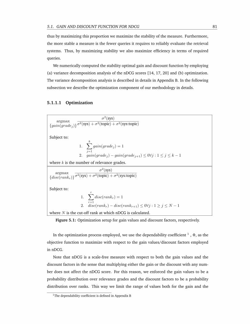
5.1. GAIN AND DISCOUNT FUNCTION FOR NDCG 81
thus by maximizing this proportion we maximize the stability of the measure. Furthermore,
the more stable a measure is the fewer queries it requires to reliably evaluate the retrieval
systems. Thus, by maximizing stability we also maximize efficiency in terms of required
queries.
We numerically computed the stability optimal gain and discount function by employing
(a) variance decomposition analysis of the nDCG scores [14, 17, 20] and (b) optimization.
The variance decomposition analysis is described in details in Appendix B. In the following
subsection we describe the optimization component of our methodology in details.
5.1.1.1 Optimization
argmax{gain(gradej)}
σ2(sys)σ2(sys) + σ2(topic) + σ2(sys:topic)
Subject to:
1.k∑
j=1
gain(gradej) = 1
2. gain(gradej)− gain(gradej+1) ≤ 0∀j : 1 ≤ j ≤ k − 1
where k is the number of relevance grades.
argmax{disc(rankr)}
σ2(sys)σ2(sys) + σ2(topic) + σ2(sys:topic)
Subject to:
1.
r∑r=1
disc(rankr) = 1
2. disc(rankr)− disc(rankr+1) ≤ 0∀j : 1 ≥ j ≤ N − 1
where N is the cut-off rank at which nDCG is calculated.
Figure 5.1: Optimization setup for gain values and discount factors, respectively.
In the optimization process employed, we use the dependability coefficient 1 , Φ, as the
objective function to maximize with respect to the gain values/discount factors employed
in nDCG.
Note that nDCG is a scale-free measure with respect to both the gain values and the
discount factors in the sense that multiplying either the gain or the discount with any num-
ber does not affect the nDCG score. For this reason, we enforced the gain values to be a
probability distribution over relevance grades and the discount factors to be a probability
distribution over ranks. This way we limit the range of values both for the gain and the
1The dependability coefficient is defined in Appendix B
82 CHAPTER 5. EVALUATION METRICS
discount within the [0, 1] range and reduce the unknown parameters by one. Furthermore,
it so happens that there maybe some fluctuation in the values of the optimal discount fac-
tors, e.g. the discount factor on a certain rank may happen to be larger than the one on
a lower rank. This is not justifiable from an IR perspective and thus, we also enforce that
the discount factors are non-increasing with the rank. The same may be true for the gain
values, hence we enforce them to be non-decreasing with the relevance grade. Further, we
set the gain value for non-relevant documents equal to zero.
Moreover, note that the coefficient Φ in Equation B.2 is a monotonically non-decreasing
function of the number of queries. In other words, the gain or discount function that is
optimal for n queries is also optimal for n + 1 queries. Therefore, in the optimization
process we set the number of queries equal to 1.
The optimization setup for the gain/discount function is mathematically expressed in
Figure 5.1. When we optimize for the discount factors we consider the gain values as given,
while when we optimize for gain values we consider the discount factors as given. We
also perform a multi-objective optimization to simultaneously optimize for the gain and
the discount function. For the purpose of the optimization, we used the fmincon MATLAB
function for the normal optimization and the minimax MATLAB function for the multi-
objective optimization. Both functions employ Sequential Quadratic Optimization.
5.1.2 Results
The afore-described optimization framework was applied to the TREC 9 and 10 Web track
collections and the TREC 12 Robust track collection. The number of participating systems
for the three collections is 105, 97 and 78 respectively. All systems were run over 50
queries2. Documents returned as a respond to these queries were judged by a single assessor
in 3 relevance grades scale: highly relevant, relevant and non-relevant. The task in all tracks
was the usual ad-hoc retrieval task.
For each one of the three test collections, we calculated the optimal discount factors
(given a linear gain function), the optimal gain values (given a logarithmic discount func-
tion) and the Pareto-optimal gain values and discount factors. We compared the optimal
gain and discount functions with the a number of commonly used gain and discount func-
tions both with respect to the stability/efficiency of the resulting nDCG measure and with
respect to the induced by the resulting nDCG ranking of systems.
2The TREC 12 Robust track collection includes 100 queries, however the first 50 of them were obtained fromTREC 6, 7 and 8, where documents were judged as either relevant or non-relevant. For this reason, we did notuse these 50 queries in our studies.
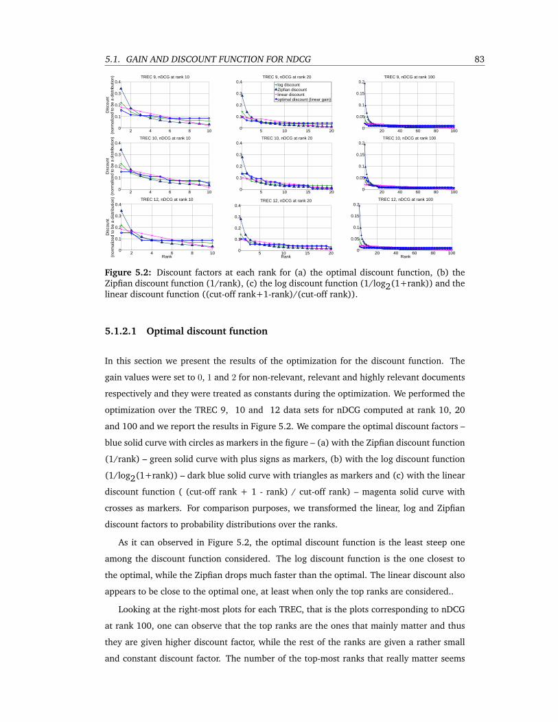
5.1. GAIN AND DISCOUNT FUNCTION FOR NDCG 83
2 4 6 8 100
0.1
0.2
0.3
0.4
Dis
coun
t(n
orm
aliz
ed to
be
a di
strib
utio
n) TREC 9, nDCG at rank 10
5 10 15 200
0.1
0.2
0.3
0.4TREC 9, nDCG at rank 20
log discountZipfian discountlinear discountoptimal discount (linear gain)
20 40 60 80 1000
0.05
0.1
0.15
0.2TREC 9, nDCG at rank 100
2 4 6 8 100
0.1
0.2
0.3
0.4
Dis
coun
t(n
orm
aliz
ed to
be
a di
strib
utio
n) TREC 10, nDCG at rank 10
5 10 15 200
0.1
0.2
0.3
0.4TREC 10, nDCG at rank 20
20 40 60 80 1000
0.05
0.1
0.15
0.2TREC 10, nDCG at rank 100
2 4 6 8 100
0.1
0.2
0.3
0.4
Dis
coun
t(n
orm
aliz
ed to
be
a di
strib
utio
n)
Rank
TREC 12, nDCG at rank 10
5 10 15 200
0.1
0.2
0.3
0.4
Rank
TREC 12, nDCG at rank 20
20 40 60 80 1000
0.05
0.1
0.15
0.2
Rank
TREC 12, nDCG at rank 100
Figure 5.2: Discount factors at each rank for (a) the optimal discount function, (b) theZipfian discount function (1/rank), (c) the log discount function (1/log2(1+rank)) and thelinear discount function ((cut-off rank+1-rank)/(cut-off rank)).
5.1.2.1 Optimal discount function
In this section we present the results of the optimization for the discount function. The
gain values were set to 0, 1 and 2 for non-relevant, relevant and highly relevant documents
respectively and they were treated as constants during the optimization. We performed the
optimization over the TREC 9, 10 and 12 data sets for nDCG computed at rank 10, 20
and 100 and we report the results in Figure 5.2. We compare the optimal discount factors –
blue solid curve with circles as markers in the figure – (a) with the Zipfian discount function
(1/rank) – green solid curve with plus signs as markers, (b) with the log discount function
(1/log2(1+rank)) – dark blue solid curve with triangles as markers and (c) with the linear
discount function ( (cut-off rank + 1 - rank) / cut-off rank) – magenta solid curve with
crosses as markers. For comparison purposes, we transformed the linear, log and Zipfian
discount factors to probability distributions over the ranks.
As it can observed in Figure 5.2, the optimal discount function is the least steep one
among the discount function considered. The log discount function is the one closest to
the optimal, while the Zipfian drops much faster than the optimal. The linear discount also
appears to be close to the optimal one, at least when only the top ranks are considered..
Looking at the right-most plots for each TREC, that is the plots corresponding to nDCG
at rank 100, one can observe that the top ranks are the ones that mainly matter and thus
they are given higher discount factor, while the rest of the ranks are given a rather small
and constant discount factor. The number of the top-most ranks that really matter seems
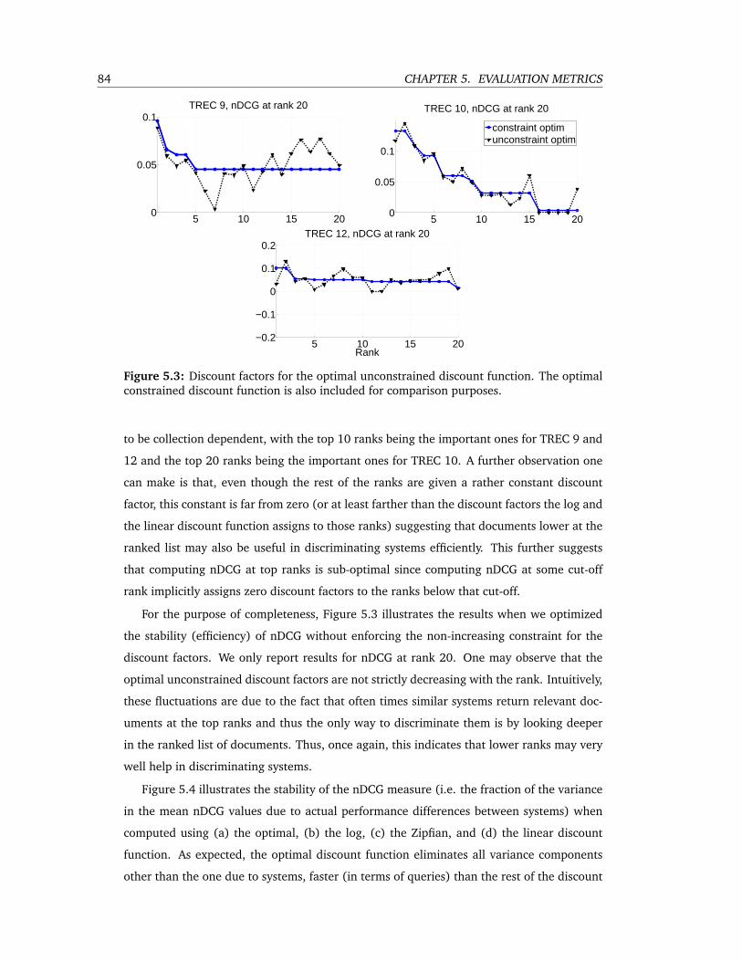
84 CHAPTER 5. EVALUATION METRICS
5 10 15 200
0.05
0.1TREC 9, nDCG at rank 20
5 10 15 200
0.05
0.1
TREC 10, nDCG at rank 20
constraint optimunconstraint optim
5 10 15 20−0.2
−0.1
0
0.1
0.2
Rank
TREC 12, nDCG at rank 20
Figure 5.3: Discount factors for the optimal unconstrained discount function. The optimalconstrained discount function is also included for comparison purposes.
to be collection dependent, with the top 10 ranks being the important ones for TREC 9 and
12 and the top 20 ranks being the important ones for TREC 10. A further observation one
can make is that, even though the rest of the ranks are given a rather constant discount
factor, this constant is far from zero (or at least farther than the discount factors the log and
the linear discount function assigns to those ranks) suggesting that documents lower at the
ranked list may also be useful in discriminating systems efficiently. This further suggests
that computing nDCG at top ranks is sub-optimal since computing nDCG at some cut-off
rank implicitly assigns zero discount factors to the ranks below that cut-off.
For the purpose of completeness, Figure 5.3 illustrates the results when we optimized
the stability (efficiency) of nDCG without enforcing the non-increasing constraint for the
discount factors. We only report results for nDCG at rank 20. One may observe that the
optimal unconstrained discount factors are not strictly decreasing with the rank. Intuitively,
these fluctuations are due to the fact that often times similar systems return relevant doc-
uments at the top ranks and thus the only way to discriminate them is by looking deeper
in the ranked list of documents. Thus, once again, this indicates that lower ranks may very
well help in discriminating systems.
Figure 5.4 illustrates the stability of the nDCG measure (i.e. the fraction of the variance
in the mean nDCG values due to actual performance differences between systems) when
computed using (a) the optimal, (b) the log, (c) the Zipfian, and (d) the linear discount
function. As expected, the optimal discount function eliminates all variance components
other than the one due to systems, faster (in terms of queries) than the rest of the discount
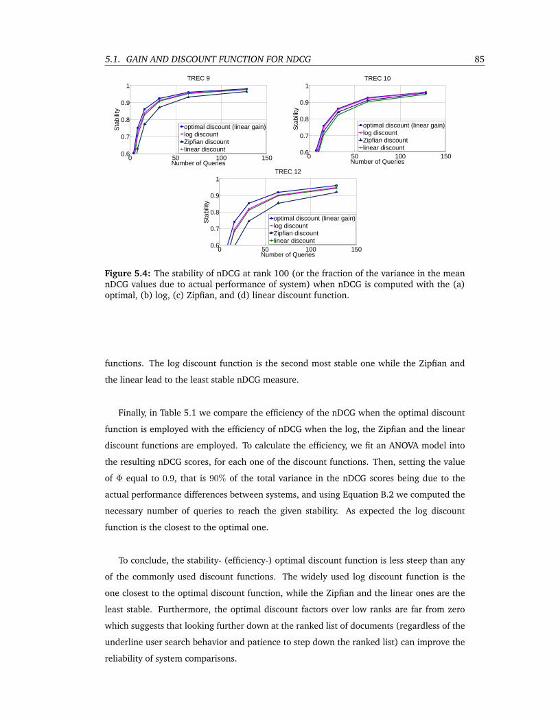
5.1. GAIN AND DISCOUNT FUNCTION FOR NDCG 85
0 50 100 1500.6
0.7
0.8
0.9
1
Number of Queries
Sta
bilit
y
TREC 9
optimal discount (linear gain)log discountZipfian discountlinear discount
0 50 100 1500.6
0.7
0.8
0.9
1
Number of Queries
Sta
bilit
y
TREC 10
optimal discount (linear gain)log discountZipfian discountlinear discount
0 50 100 1500.6
0.7
0.8
0.9
1
Number of Queries
Sta
bilit
y
TREC 12
optimal discount (linear gain)log discountZipfian discountlinear discount
Figure 5.4: The stability of nDCG at rank 100 (or the fraction of the variance in the meannDCG values due to actual performance of system) when nDCG is computed with the (a)optimal, (b) log, (c) Zipfian, and (d) linear discount function.
functions. The log discount function is the second most stable one while the Zipfian and
the linear lead to the least stable nDCG measure.
Finally, in Table 5.1 we compare the efficiency of the nDCG when the optimal discount
function is employed with the efficiency of nDCG when the log, the Zipfian and the linear
discount functions are employed. To calculate the efficiency, we fit an ANOVA model into
the resulting nDCG scores, for each one of the discount functions. Then, setting the value
of Φ equal to 0.9, that is 90% of the total variance in the nDCG scores being due to the
actual performance differences between systems, and using Equation B.2 we computed the
necessary number of queries to reach the given stability. As expected the log discount
function is the closest to the optimal one.
To conclude, the stability- (efficiency-) optimal discount function is less steep than any
of the commonly used discount functions. The widely used log discount function is the
one closest to the optimal discount function, while the Zipfian and the linear ones are the
least stable. Furthermore, the optimal discount factors over low ranks are far from zero
which suggests that looking further down at the ranked list of documents (regardless of the
underline user search behavior and patience to step down the ranked list) can improve the
reliability of system comparisons.
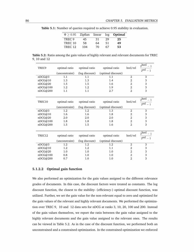
86 CHAPTER 5. EVALUATION METRICS
Table 5.1: Number of queries required to achieve 0.95 stability in evaluation.
Φ ≥ 0.95 Zipfian linear log OptimalTREC 9 45 31 29 25TREC 10 58 64 51 49TREC 12 104 70 67 53
Table 5.2: Ratio among the gain values of highly relevant and relevant documents for TREC9, 10 and 12
TREC9 optimal ratio optimal ratio optimal ratio hrel/rel2hrel − 1
2rel − 1(unconstraint) (log discount) (optimal discount)
nDCG@3 1.1 1.1 1.1 2 3nDCG@10 1.3 1.3 1.4 2 3nDCG@20 1.5 1.5 1.6 2 3nDCG@100 1.2 1.2 1.9 2 3nDCG@200 1.1 1.1 2.7 2 3
TREC10 optimal ratio optimal ratio optimal ratio hrel/rel2hrel − 1
2rel − 1(unconstraint) (log discount) (optimal discount)
nDCG@3 1.2 1.2 1.3 2 3nDCG@10 1.6 1.6 1.8 2 3nDCG@20 2.0 2.0 2.0 2 3nDCG@100 1.8 1.8 1.8 2 3nDCG@200 1.5 1.5 1.6 2 3
TREC12 optimal ratio optimal ratio optimal ratio hrel/rel2hrel − 1
2rel − 1(unconstraint) (log discount) (optimal discount)
nDCG@3 1.2 1.2 1.2 2 3nDCG@10 1.2 1.2 1.1 2 3nDCG@20 1.0 1.0 1.0 2 3nDCG@100 0.8 1.0 1.0 2 3nDCG@200 0.7 1.0 1.0 2 3
5.1.2.2 Optimal gain function
We also performed an optimization for the gain values assigned to the different relevance
grades of documents. In this case, the discount factors were treated as constants. The log
discount function, the closest to the stability- (efficiency-) optimal discount function, was
utilized. Further, we set the gain value for the non-relevant equal to zero and optimized for
the gain values of the relevant and highly relevant documents. We performed the optimiza-
tion over TREC 9, 10 and 12 data sets for nDCG at ranks 3, 10, 20, 100 and 200. Instead
of the gain values themselves, we report the ratio between the gain value assigned to the
highly relevant documents and the gain value assigned to the relevant ones. The results
can be viewed in Table 5.2. As in the case of the discount function, we performed both an
unconstrained and a constrained optimization. In the constrained optimization we enforced
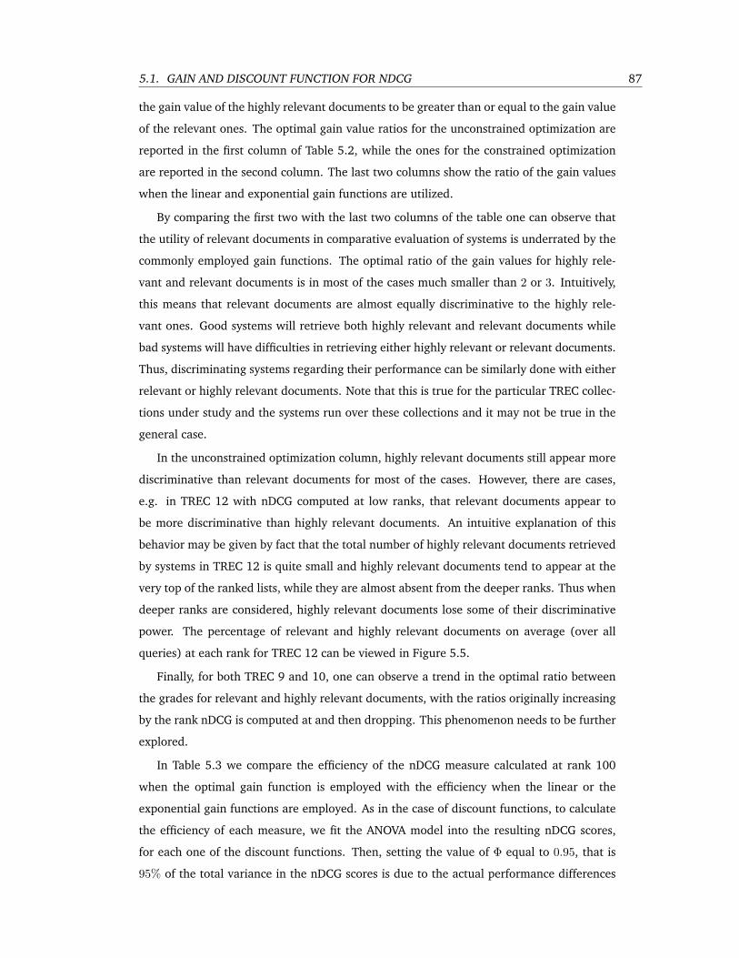
5.1. GAIN AND DISCOUNT FUNCTION FOR NDCG 87
the gain value of the highly relevant documents to be greater than or equal to the gain value
of the relevant ones. The optimal gain value ratios for the unconstrained optimization are
reported in the first column of Table 5.2, while the ones for the constrained optimization
are reported in the second column. The last two columns show the ratio of the gain values
when the linear and exponential gain functions are utilized.
By comparing the first two with the last two columns of the table one can observe that
the utility of relevant documents in comparative evaluation of systems is underrated by the
commonly employed gain functions. The optimal ratio of the gain values for highly rele-
vant and relevant documents is in most of the cases much smaller than 2 or 3. Intuitively,
this means that relevant documents are almost equally discriminative to the highly rele-
vant ones. Good systems will retrieve both highly relevant and relevant documents while
bad systems will have difficulties in retrieving either highly relevant or relevant documents.
Thus, discriminating systems regarding their performance can be similarly done with either
relevant or highly relevant documents. Note that this is true for the particular TREC collec-
tions under study and the systems run over these collections and it may not be true in the
general case.
In the unconstrained optimization column, highly relevant documents still appear more
discriminative than relevant documents for most of the cases. However, there are cases,
e.g. in TREC 12 with nDCG computed at low ranks, that relevant documents appear to
be more discriminative than highly relevant documents. An intuitive explanation of this
behavior may be given by fact that the total number of highly relevant documents retrieved
by systems in TREC 12 is quite small and highly relevant documents tend to appear at the
very top of the ranked lists, while they are almost absent from the deeper ranks. Thus when
deeper ranks are considered, highly relevant documents lose some of their discriminative
power. The percentage of relevant and highly relevant documents on average (over all
queries) at each rank for TREC 12 can be viewed in Figure 5.5.
Finally, for both TREC 9 and 10, one can observe a trend in the optimal ratio between
the grades for relevant and highly relevant documents, with the ratios originally increasing
by the rank nDCG is computed at and then dropping. This phenomenon needs to be further
explored.
In Table 5.3 we compare the efficiency of the nDCG measure calculated at rank 100
when the optimal gain function is employed with the efficiency when the linear or the
exponential gain functions are employed. As in the case of discount functions, to calculate
the efficiency of each measure, we fit the ANOVA model into the resulting nDCG scores,
for each one of the discount functions. Then, setting the value of Φ equal to 0.95, that is
95% of the total variance in the nDCG scores is due to the actual performance differences
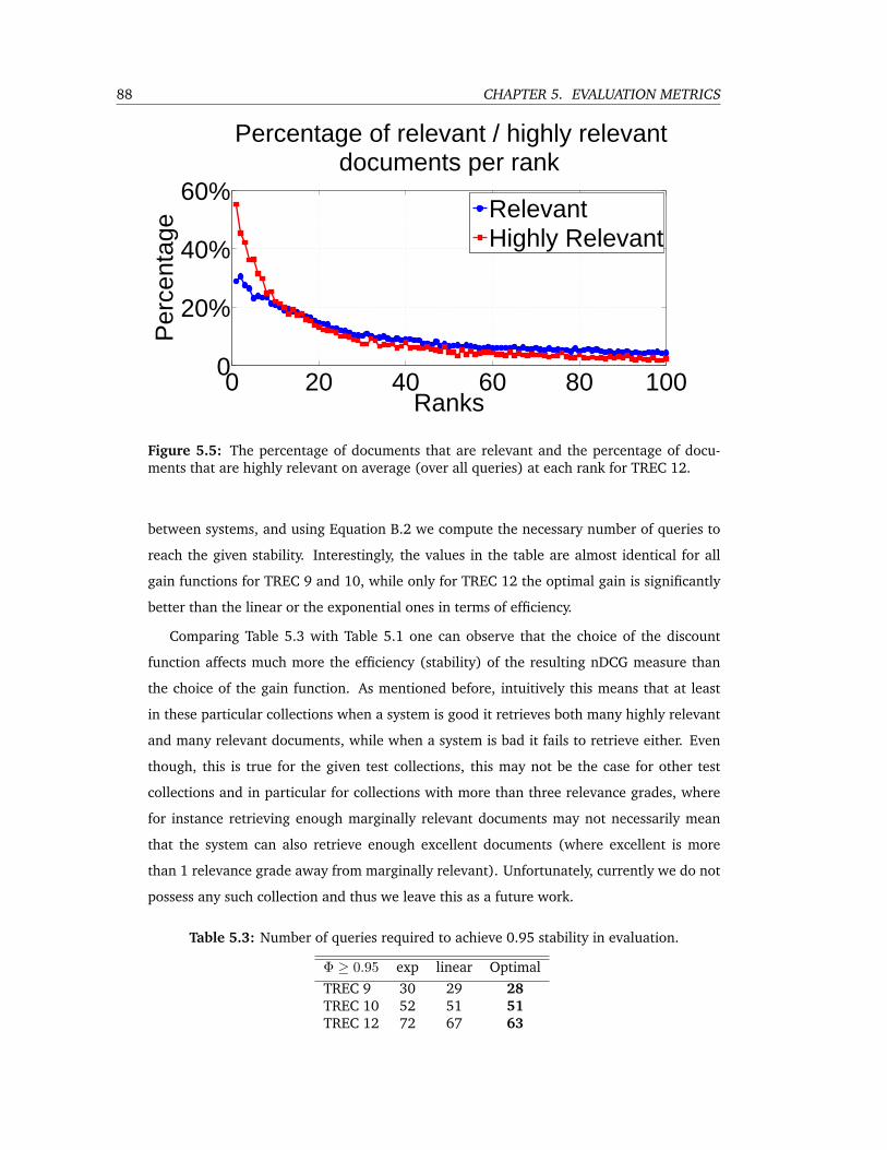
88 CHAPTER 5. EVALUATION METRICS
0 20 40 60 80 1000
20%
40%
60%
Ranks
Per
cent
age
Percentage of relevant / highly relevantdocuments per rank
RelevantHighly Relevant
Figure 5.5: The percentage of documents that are relevant and the percentage of docu-ments that are highly relevant on average (over all queries) at each rank for TREC 12.
between systems, and using Equation B.2 we compute the necessary number of queries to
reach the given stability. Interestingly, the values in the table are almost identical for all
gain functions for TREC 9 and 10, while only for TREC 12 the optimal gain is significantly
better than the linear or the exponential ones in terms of efficiency.
Comparing Table 5.3 with Table 5.1 one can observe that the choice of the discount
function affects much more the efficiency (stability) of the resulting nDCG measure than
the choice of the gain function. As mentioned before, intuitively this means that at least
in these particular collections when a system is good it retrieves both many highly relevant
and many relevant documents, while when a system is bad it fails to retrieve either. Even
though, this is true for the given test collections, this may not be the case for other test
collections and in particular for collections with more than three relevance grades, where
for instance retrieving enough marginally relevant documents may not necessarily mean
that the system can also retrieve enough excellent documents (where excellent is more
than 1 relevance grade away from marginally relevant). Unfortunately, currently we do not
possess any such collection and thus we leave this as a future work.
Table 5.3: Number of queries required to achieve 0.95 stability in evaluation.
Φ ≥ 0.95 exp linear OptimalTREC 9 30 29 28TREC 10 52 51 51TREC 12 72 67 63
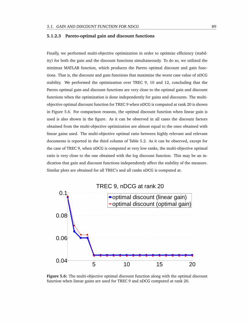
5.1. GAIN AND DISCOUNT FUNCTION FOR NDCG 89
5.1.2.3 Pareto-optimal gain and discount functions
Finally, we performed multi-objective optimization in order to optimize efficiency (stabil-
ity) for both the gain and the discount functions simultaneously. To do so, we utilized the
minimax MATLAB function, which produces the Pareto optimal discount and gain func-
tions. That is, the discount and gain functions that maximize the worst case value of nDCG
stability. We performed the optimization over TREC 9, 10 and 12, concluding that the
Pareto optimal gain and discount functions are very close to the optimal gain and discount
functions when the optimization is done independently for gains and discounts. The multi-
objective optimal discount function for TREC 9 when nDCG is computed at rank 20 is shown
in Figure 5.6. For comparison reasons, the optimal discount function when linear gain is
used is also shown in the figure. As it can be observed in all cases the discount factors
obtained from the multi-objective optimization are almost equal to the ones obtained with
linear gains used. The multi-objective optimal ratio between highly relevant and relevant
documents is reported in the third column of Table 5.2. As it can be observed, except for
the case of TREC 9, when nDCG is computed at very low ranks, the multi-objective optimal
ratio is very close to the one obtained with the log discount function. This may be an in-
dication that gain and discount functions independently affect the stability of the measure.
Similar plots are obtained for all TREC’s and all ranks nDCG is computed at.
5 10 15 200.04
0.06
0.08
0.1TREC 9, nDCG at rank 20
optimal discount (linear gain)optimal discount (optimal gain)
Figure 5.6: The multi-objective optimal discount function along with the optimal discountfunction when linear gains are used for TREC 9 and nDCG computed at rank 20.
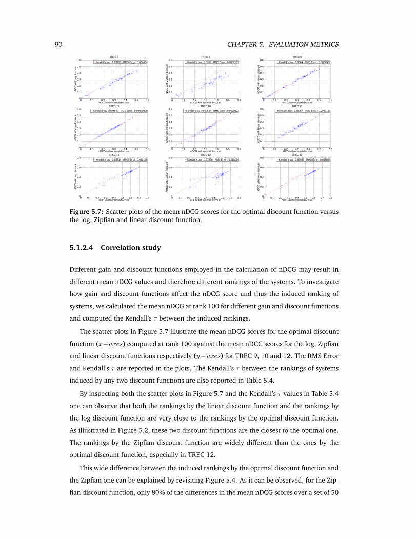
90 CHAPTER 5. EVALUATION METRICS
0 0.1 0.2 0.3 0.4 0.5 0.60
0.1
0.2
0.3
0.4
0.5
0.6
nDCG with optimal discount
nDC
G w
ith lo
g di
scou
nt
TREC 9
Kendall’s tau : 0.93735 RMS Error : 0.004424
0 0.1 0.2 0.3 0.4 0.5 0.60
0.1
0.2
0.3
0.4
0.5
0.6
nDCG with optimal discount
nDC
G w
ith Z
ipfia
n di
scou
nt
TREC 9
Kendall’s tau : 0.8355 RMS Error : 0.0082557
0 0.1 0.2 0.3 0.4 0.5 0.60
0.1
0.2
0.3
0.4
0.5
0.6
nDCG with optimal discount
nDC
G w
ith li
near
dis
coun
t
TREC 9
Kendall’s tau : 0.9564 RMS Error : 0.0082557
0 0.1 0.2 0.3 0.4 0.5 0.60
0.1
0.2
0.3
0.4
0.5
0.6
nDCG with optimal discount
nDC
G w
ith lo
g di
scou
nt
TREC 10
Kendall’s tau : 0.94532 RMS Error : 0.00089939
0 0.1 0.2 0.3 0.4 0.5 0.60
0.1
0.2
0.3
0.4
0.5
0.6
nDCG with optimal discount
nDC
G w
ith Z
ipfia
n di
scou
nt
TREC 10
Kendall’s tau : 0.89548 RMS Error : 0.0030133
0 0.1 0.2 0.3 0.4 0.5 0.60
0.1
0.2
0.3
0.4
0.5
0.6
nDCG with optimal discount
nDC
G w
ith li
near
dis
coun
t
TREC 10
Kendall’s tau : 0.88087 RMS Error : 0.0030133
0 0.1 0.2 0.3 0.4 0.5 0.6 0.7 0.80
0.2
0.4
0.6
0.8
nDCG with optimal discount
nDC
G w
ith lo
g di
scou
nt
TREC 12
Kendall’s tau : 0.85814 RMS Error : 0.010159
0 0.1 0.2 0.3 0.4 0.5 0.6 0.7 0.80
0.2
0.4
0.6
0.8
nDCG with optimal discount
nDC
G w
ith Z
ipfia
n di
scou
nt
TREC 12
Kendall’s tau : 0.67566 RMS Error : 0.018024
0 0.1 0.2 0.3 0.4 0.5 0.6 0.7 0.80
0.2
0.4
0.6
0.8
nDCG with optimal discount
nDC
G w
ith li
near
dis
coun
t
TREC 12
Kendall’s tau : 0.89943 RMS Error : 0.018024
Figure 5.7: Scatter plots of the mean nDCG scores for the optimal discount function versusthe log, Zipfian and linear discount function.
5.1.2.4 Correlation study
Different gain and discount functions employed in the calculation of nDCG may result in
different mean nDCG values and therefore different rankings of the systems. To investigate
how gain and discount functions affect the nDCG score and thus the induced ranking of
systems, we calculated the mean nDCG at rank 100 for different gain and discount functions
and computed the Kendall’s τ between the induced rankings.
The scatter plots in Figure 5.7 illustrate the mean nDCG scores for the optimal discount
function (x−axes) computed at rank 100 against the mean nDCG scores for the log, Zipfian
and linear discount functions respectively (y−axes) for TREC 9, 10 and 12. The RMS Error
and Kendall’s τ are reported in the plots. The Kendall’s τ between the rankings of systems
induced by any two discount functions are also reported in Table 5.4.
By inspecting both the scatter plots in Figure 5.7 and the Kendall’s τ values in Table 5.4
one can observe that both the rankings by the linear discount function and the rankings by
the log discount function are very close to the rankings by the optimal discount function.
As illustrated in Figure 5.2, these two discount functions are the closest to the optimal one.
The rankings by the Zipfian discount function are widely different than the ones by the
optimal discount function, especially in TREC 12.
This wide difference between the induced rankings by the optimal discount function and
the Zipfian one can be explained by revisiting Figure 5.4. As it can be observed, for the Zip-
fian discount function, only 80% of the differences in the mean nDCG scores over a set of 50
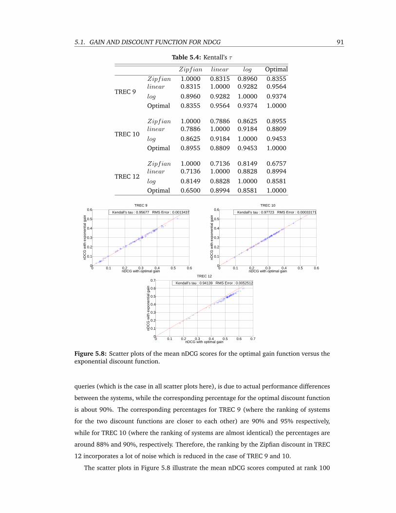
5.1. GAIN AND DISCOUNT FUNCTION FOR NDCG 91
Table 5.4: Kentall’s τ
Zipfian linear log OptimalZipfian 1.0000 0.8315 0.8960 0.8355linear 0.8315 1.0000 0.9282 0.9564
TREC 9log 0.8960 0.9282 1.0000 0.9374Optimal 0.8355 0.9564 0.9374 1.0000
Zipfian 1.0000 0.7886 0.8625 0.8955linear 0.7886 1.0000 0.9184 0.8809
TREC 10log 0.8625 0.9184 1.0000 0.9453Optimal 0.8955 0.8809 0.9453 1.0000
Zipfian 1.0000 0.7136 0.8149 0.6757linear 0.7136 1.0000 0.8828 0.8994
TREC 12log 0.8149 0.8828 1.0000 0.8581Optimal 0.6500 0.8994 0.8581 1.0000
0 0.1 0.2 0.3 0.4 0.5 0.60
0.1
0.2
0.3
0.4
0.5
0.6
nDCG with optimal gain
nDC
G w
ith e
xpon
entia
l gai
n
TREC 9
Kendall’s tau : 0.95677 RMS Error : 0.0013437
0 0.1 0.2 0.3 0.4 0.5 0.60
0.1
0.2
0.3
0.4
0.5
0.6
nDCG with optimal gain
nDC
G w
ith e
xpon
entia
l gai
n
TREC 10
Kendall’s tau : 0.97723 RMS Error : 0.00033171
0 0.1 0.2 0.3 0.4 0.5 0.6 0.70
0.1
0.2
0.3
0.4
0.5
0.6
0.7
nDCG with optimal gain
nDC
G w
ith e
xpon
entia
l gai
n
TREC 12
Kendall’s tau : 0.94139 RMS Error : 0.0052512
Figure 5.8: Scatter plots of the mean nDCG scores for the optimal gain function versus theexponential discount function.
queries (which is the case in all scatter plots here), is due to actual performance differences
between the systems, while the corresponding percentage for the optimal discount function
is about 90%. The corresponding percentages for TREC 9 (where the ranking of systems
for the two discount functions are closer to each other) are 90% and 95% respectively,
while for TREC 10 (where the ranking of systems are almost identical) the percentages are
around 88% and 90%, respectively. Therefore, the ranking by the Zipfian discount in TREC
12 incorporates a lot of noise which is reduced in the case of TREC 9 and 10.
The scatter plots in Figure 5.8 illustrate the mean nDCG scores computed at rank 100
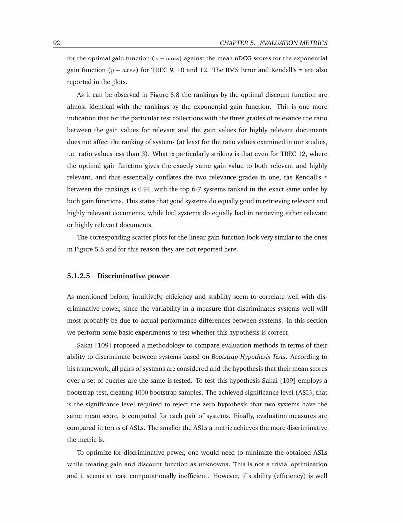
92 CHAPTER 5. EVALUATION METRICS
for the optimal gain function (x− axes) against the mean nDCG scores for the exponential
gain function (y − axes) for TREC 9, 10 and 12. The RMS Error and Kendall’s τ are also
reported in the plots.
As it can be observed in Figure 5.8 the rankings by the optimal discount function are
almost identical with the rankings by the exponential gain function. This is one more
indication that for the particular test collections with the three grades of relevance the ratio
between the gain values for relevant and the gain values for highly relevant documents
does not affect the ranking of systems (at least for the ratio values examined in our studies,
i.e. ratio values less than 3). What is particularly striking is that even for TREC 12, where
the optimal gain function gives the exactly same gain value to both relevant and highly
relevant, and thus essentially conflates the two relevance grades in one, the Kendall’s τ
between the rankings is 0.94, with the top 6-7 systems ranked in the exact same order by
both gain functions. This states that good systems do equally good in retrieving relevant and
highly relevant documents, while bad systems do equally bad in retrieving either relevant
or highly relevant documents.
The corresponding scatter plots for the linear gain function look very similar to the ones
in Figure 5.8 and for this reason they are not reported here.
5.1.2.5 Discriminative power
As mentioned before, intuitively, efficiency and stability seem to correlate well with dis-
criminative power, since the variability in a measure that discriminates systems well will
most probably be due to actual performance differences between systems. In this section
we perform some basic experiments to test whether this hypothesis is correct.
Sakai [109] proposed a methodology to compare evaluation methods in terms of their
ability to discriminate between systems based on Bootstrap Hypothesis Tests. According to
his framework, all pairs of systems are considered and the hypothesis that their mean scores
over a set of queries are the same is tested. To test this hypothesis Sakai [109] employs a
bootstrap test, creating 1000 bootstrap samples. The achieved significance level (ASL), that
is the significance level required to reject the zero hypothesis that two systems have the
same mean score, is computed for each pair of systems. Finally, evaluation measures are
compared in terms of ASLs. The smaller the ASLs a metric achieves the more discriminative
the metric is.
To optimize for discriminative power, one would need to minimize the obtained ASLs
while treating gain and discount function as unknowns. This is not a trivial optimization
and it seems at least computationally inefficient. However, if stability (efficiency) is well
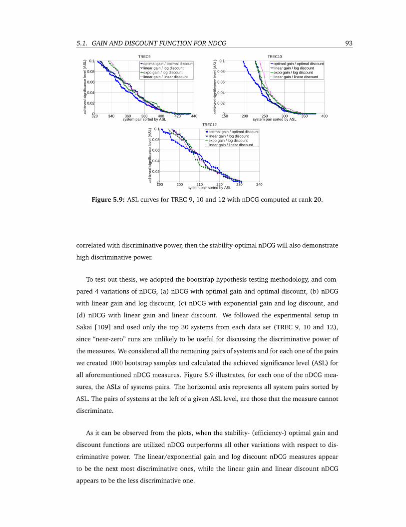
5.1. GAIN AND DISCOUNT FUNCTION FOR NDCG 93
320 340 360 380 400 420 4400
0.02
0.04
0.06
0.08
0.1
system pair sorted by ASL
achi
eved
sig
nific
ance
leve
l (A
SL)
TREC9
optimal gain / optimal discountlinear gain / log discountexpo gain / log discountlinear gain / linear discount
150 200 250 300 350 4000
0.02
0.04
0.06
0.08
0.1
system pair sorted by ASL
achi
eved
sig
nific
ance
leve
l (A
SL)
TREC10
optimal gain / optimal discountlinear gain / log discountexpo gain / log discountlinear gain / linear discount
190 200 210 220 230 2400
0.02
0.04
0.06
0.08
0.1
system pair sorted by ASL
achi
eved
sig
nific
ance
leve
l (A
SL)
TREC12
optimal gain / optimal discountlinear gain / log discountexpo gain / log discountlinear gain / linear discount
Figure 5.9: ASL curves for TREC 9, 10 and 12 with nDCG computed at rank 20.
correlated with discriminative power, then the stability-optimal nDCG will also demonstrate
high discriminative power.
To test out thesis, we adopted the bootstrap hypothesis testing methodology, and com-
pared 4 variations of nDCG, (a) nDCG with optimal gain and optimal discount, (b) nDCG
with linear gain and log discount, (c) nDCG with exponential gain and log discount, and
(d) nDCG with linear gain and linear discount. We followed the experimental setup in
Sakai [109] and used only the top 30 systems from each data set (TREC 9, 10 and 12),
since “near-zero” runs are unlikely to be useful for discussing the discriminative power of
the measures. We considered all the remaining pairs of systems and for each one of the pairs
we created 1000 bootstrap samples and calculated the achieved significance level (ASL) for
all aforementioned nDCG measures. Figure 5.9 illustrates, for each one of the nDCG mea-
sures, the ASLs of systems pairs. The horizontal axis represents all system pairs sorted by
ASL. The pairs of systems at the left of a given ASL level, are those that the measure cannot
discriminate.
As it can be observed from the plots, when the stability- (efficiency-) optimal gain and
discount functions are utilized nDCG outperforms all other variations with respect to dis-
criminative power. The linear/exponential gain and log discount nDCG measures appear
to be the next most discriminative ones, while the linear gain and linear discount nDCG
appears to be the less discriminative one.

94 CHAPTER 5. EVALUATION METRICS
5.1.3 Conclusions
Despite the flexibility nDCG offers in the selection of the appropriate gain and discount
function, so far this selection has been done rather arbitrarily, based on speculations of
the search behavior of an average user and speculations of the correlation of the measure
to user satisfaction. Recent work [1] has shown that the most commonly employed gain
and discount functions are loosely related to user satisfaction which underlines the need
for a more methodological selection of gain and discount function. However, given the
infinite number of possible gain and discount functions, the vast differences in user search
behavior, the many different possible retrieval tasks, a complete analysis of the different
gain and discount functions with respect to the user satisfaction is prohibitively expensive,
if at all possible.
In this work, we numerically computed a stability- or efficiency-optimal gain and dis-
count function by treating gain values and discount factors as unknowns and optimizing for
a stability/efficiency measure defined based on Generalizability theory. We compared the
resulting gain function to both the linear and the exponential functions and the resulting
discount function to the log, Zipfian and linear ones.
According to our results, the optimal discount function is less steep than all commonly
used discount functions, giving reasonably high weights to lower ranks, while the relative
difference between gain values is much smaller than the commonly used ones, giving al-
most equal weights to both relevant and highly relevant documents. The latter was rather
striking, since weighting relevant and highly relevant documents equally did not seem to
alter the ranking of systems. Note that this is true for the particular collections and systems
under study and it may not reflect the general case.
Finally, we demonstrated that the stability- (efficiency-) optimal nDCG measure outper-
forms the dominant in the literature nDCG measure with respect to discriminative power as
well.

5.2. EXTENSION OF AVERAGE PRECISION TO GRADED RELEVANCE JUDGMENTS 95
5.2 Extension of Average Precision to Graded Relevance Judgments
Given that average precision remains one of the most popular metric of effectiveness, here
we generalize average precision to the multigraded relevance case in a systematic manner,
proposing a new metric, the graded average precision (GAP). The GAP metric is a direct
extension of AP and thus it inherits all the desirable properties that average precision has:
• It has the same natural top-heavy bias average precision has.
• It has a nice probabilistic interpretation.
• It has an underlying theoretical basis as it corresponds to the area under the ”graded”
precision-recall curve.
• It can be justified in terms of a simple but moderately plausible user model similarly
to AP
• It appears to be highly informative.
• When used as an objective function in learning-to-rank it results in good performance
retrieval systems (it outperforms both AP and nDCG).
The incorporation of multi-graded relevance in average precision becomes possible via
a simple probabilistic user model which naturally dictates to what extend documents of
different relevance grades account for the effectiveness score. This user model corresponds
to one of the approaches briefly discussed in Sakai and Robertson [112]. This model offers
an alternative way of thinking about graded relevance compared to the notion of utility
employed by nDCG and other multi-graded metrics.
Sakai [111] introduced the Q-measure as a better mechanism to control the penalty to
late arrivals of relevant documents than nDCG. It has been shown that for ranks above R
Q-measure behaves similarly to AP (where R is the number of relevant documents in the
collection). Nevertheless, the incorporation of graded relevance by the Q-measure follows
the same model with nDCG. GAP, on the other hand, is based on the well-trusted notions
of precision and recall as is AP. Thus, we propose GAP as a complement to the existing
multi-graded metrics.
In this work we do not aim at proposing a family of measures that accommodate differ-
ent user behavior, as is nDCG (even though GAP offers some flexibility). Instead, by gen-
eralizing average precision we propose a more system-oriented measure, that apart from
comparing the overall performance of retrieval systems in a similar to average precision
way, it can be utilized in the critical task of learning to rank and improve the performance
of the resulting ranking functions.
96 CHAPTER 5. EVALUATION METRICS
In what follows, we first describe the user model on which GAP is based and define
the new metric. We then describe some desirable properties GAP possesses. In particular,
we describe a probabilistic interpretation of GAP, generalize precision-recall curves for the
multigraded relevance case and show that GAP is an approximation to the area under the
graded precision-recall curves. Further, we evaluate GAP in terms of informativeness [10]
and discriminative power [109]. Finally, we extend two popular LTR algorithms, Soft-
Rank [129] and LambdaRank [27], to optimize for GAP and test the performance of the
resulting ranking functions over different collections.
5.2.1 Graded Average Precision (GAP)
5.2.1.1 User Model
We start from a rudimentary user model, as follows: assume that the user actually has a bi-
nary view of relevance, determined by thresholding the relevance scale {0..c}. We describe
this model probabilistically – we have a probability gi that the user sets the threshold at
grade i, in other words regards grades i, ..., c as relevant and the others as non-relevant. We
consider this probability to be defined over the space of users. These should be exclusive
and exhaustive probabilities:∑c
j=1 gj = 1.
5.2.1.2 Definition of GAP
Now, we want some form of expected average precision, the expectation being over this
afore-defined probabilistic event space. Simple interpretation of this (just calculate average
precision separately for each grade and take a probabilistically weighted combination) has
problems; for instance, in the case of an ideal ranked list, when there are no documents in
some grades, the effectiveness score returned is less than the optimal value of 1. So, instead,
we extend the non-interpolated form of AP; that is, we step down the ranked list, looking at
each relevant document in turn (the ”pivot” document) and compute the expected precision
at this rank. With an appropriate normalization at the end, this defines the graded average
precision (GAP).
In particular, suppose we have a ranked list of documents, and document dn at rank n
has relevance in ∈ {0..c}. If in > 0, dn, as pivot document, will contribute a precision value
to the average precision calculations for each grade j, 0 < j ≤ in, since for any threshold
set at grades less than or equal to in, dn is considered relevant. The binary precision value
for each grade j is, 1n (|dm : m ≤ n, im ≥ j|), while the expected precision at rank n over
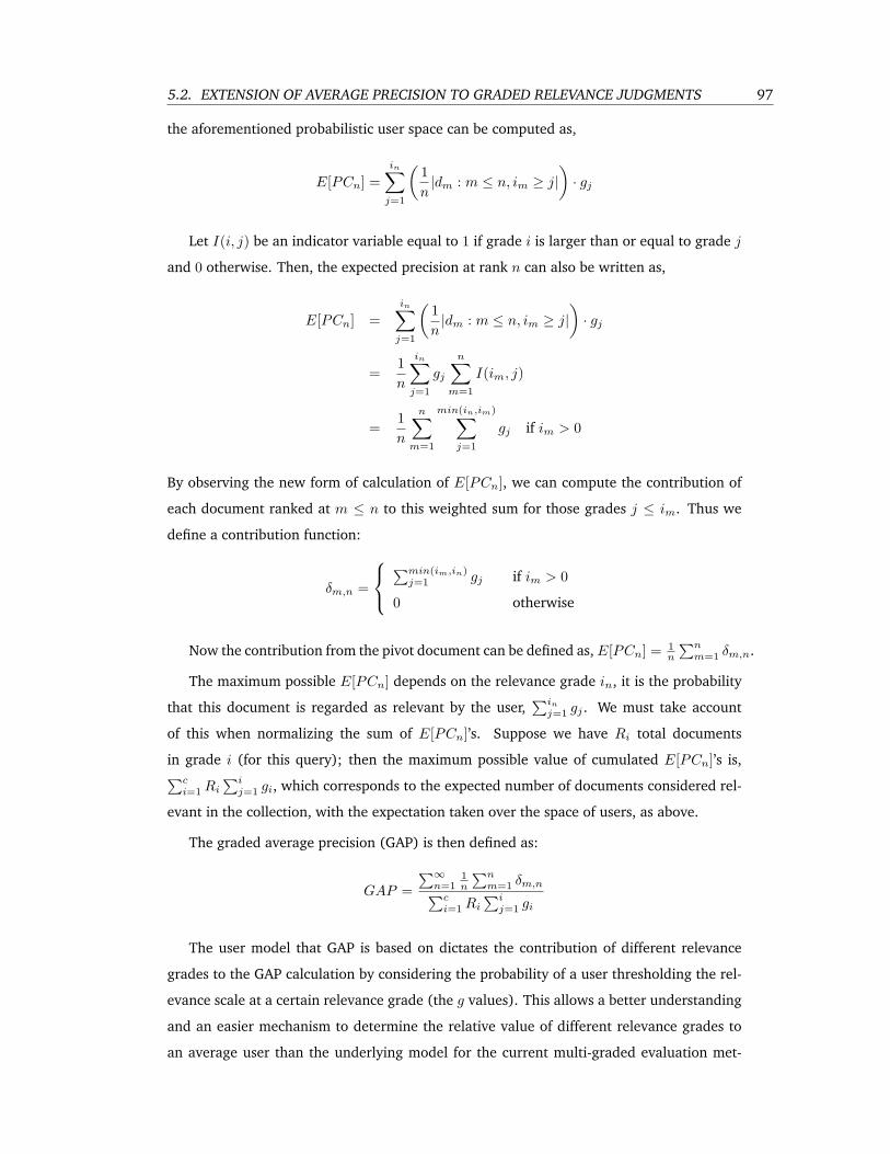
5.2. EXTENSION OF AVERAGE PRECISION TO GRADED RELEVANCE JUDGMENTS 97
the aforementioned probabilistic user space can be computed as,
E[PCn] =in∑
j=1
(1n|dm : m ≤ n, im ≥ j|
)· gj
Let I(i, j) be an indicator variable equal to 1 if grade i is larger than or equal to grade j
and 0 otherwise. Then, the expected precision at rank n can also be written as,
E[PCn] =in∑
j=1
(1n|dm : m ≤ n, im ≥ j|
)· gj
=1n
in∑j=1
gj
n∑m=1
I(im, j)
=1n
n∑m=1
min(in,im)∑j=1
gj if im > 0
By observing the new form of calculation of E[PCn], we can compute the contribution of
each document ranked at m ≤ n to this weighted sum for those grades j ≤ im. Thus we
define a contribution function:
δm,n =
∑min(im,in)
j=1 gj if im > 0
0 otherwise
Now the contribution from the pivot document can be defined as, E[PCn] = 1n
∑nm=1 δm,n.
The maximum possible E[PCn] depends on the relevance grade in, it is the probability
that this document is regarded as relevant by the user,∑in
j=1 gj . We must take account
of this when normalizing the sum of E[PCn]’s. Suppose we have Ri total documents
in grade i (for this query); then the maximum possible value of cumulated E[PCn]’s is,∑ci=1 Ri
∑ij=1 gi, which corresponds to the expected number of documents considered rel-
evant in the collection, with the expectation taken over the space of users, as above.
The graded average precision (GAP) is then defined as:
GAP =∑∞
n=11n
∑nm=1 δm,n∑c
i=1 Ri
∑ij=1 gi
The user model that GAP is based on dictates the contribution of different relevance
grades to the GAP calculation by considering the probability of a user thresholding the rel-
evance scale at a certain relevance grade (the g values). This allows a better understanding
and an easier mechanism to determine the relative value of different relevance grades to
an average user than the underlying model for the current multi-graded evaluation met-
98 CHAPTER 5. EVALUATION METRICS
rics. For instance, given the relevance grades of documents, click through data can be
utilized to conclude relative preferences of users among documents of different relevance
grades [72, 84]. Assuming that the user only clicks on the documents he finds relevant,
the g values correspond to the probability that a user clicks on a document of a particular
relevance grade, given all the documents clicked by the user.
In this work, given that our goal is to develop a good system-oriented metric, we propose
an alternative way of setting the g values by considering which g = {gi} makes the metric
most informative 5.2.3.1.
5.2.2 Properties of GAP
In this section, we describe some of the properties of GAP and show that GAP inherits all
the nice properties of average precision (extended to the multi-graded case) that make the
metric understandable and desirable to use.
First, it is easy to see that GAP generalizes average precision – it reverts to average preci-
sion in the case of binary relevance. With respect to the model described in Section 5.2.1.1,
binary relevance means that all users find documents with some relevance grade t > 0 rel-
evant and the rest non-relevant (i.e., gj = 1 if j = t, for some relevance grade t > 0 and 0
otherwise).
Furthermore, GAP behaves in the expected way under document swaps. That is, if
a document is swapped with another document of smaller relevance grade that appears
lower in the list, the value of GAP decreases and vice-versa. As a corollary to this property,
GAP acquires its maximum value when documents are returned in non-increasing relevance
grade order.
Finally, GAP possesses all the desirable properties of average precision:
• It has the natural top-heavy bias of average precision and so it does not require explicit
discount function.
• It has a nice probabilistic interpretation (Section 5.2.2.1).
• It approximates the area under a ’graded’ precision-recall curve (Section 5.2.2.2).
• It is highly informative (Section 5.2.3).
In the following sections, we describe a probabilistic interpretation of GAP and show that
GAP is an approximation to the area under a graded precision-recall curve.

5.2. EXTENSION OF AVERAGE PRECISION TO GRADED RELEVANCE JUDGMENTS 99
5.2.2.1 Probabilistic interpretation
In this section, we describe the probabilistic interpretation of GAP. We show that GAP can
be seen as a probability value, which makes the measure more intuitive. In particular, we
define GAP as the expected outcome of a random experiment, which is a generalization of
the random experiment whose expected outcome is average precision [146], for the case of
graded relevance.
Probabilistic interpretation of AP: Recently, Yilmaz and Aslam [146] showed that AP
corresponds to the expected outcome of the following random experiment:
1. Select a relevant document at random. Let the rank of this document be n.
2. Select a document at or above rank n, at random. Let the rank of that document be
m.
3. Output 1 if the document at rank m, dm, is relevant.
In expectation, steps (2) and (3) effectively compute the precision at a relevant docu-
ment, and in combination, step (1) effectively computes the average of these precisions.
Hence, average precision corresponds to the probability that a document retrieved above a
randomly picked relevant document is also relevant.
Probabilistic interpretation of GAP: Consider the case where graded relevance judg-
ments are available. We claim that GAP corresponds to the expected outcome of the follow-
ing random experiment:
1. Select a document that is considered relevant by a user (according to the afore-defined
user model), at random. Let the rank of this document be n.
2. Select a document at or above rank n, at random. Let the rank of that document be
m.
3. Output 1 if the document at rank m, dm, is also considered relevant by the user.
Hence, GAP can be seen as the probability that a document retrieved above a randomly
picked ’relevant’ document is also ’relevant’, where relevance is defined according to the
user model previously described.
Consider computing the expectation of the above random experiment to show that it
corresponds to GAP.
In expectation, step (3) corresponds to the conditional probability of document dm being
considered as relevant given that document dn is also considered as relevant. To calculate
100 CHAPTER 5. EVALUATION METRICS
this probability, let’s consider all possible cases of the relative ordering of the relevant grades
for documents dn and dm.
• (in ≤ im) : Since the relevance grade of dn is smaller than or equal to the one for dm,
if dn is considered relevant then dm will also be considered as relevant.
Pr(dm = rel|dn = rel) =
= 1 =
∑in
j=1 gj∑in
j=1 gj
=
∑min(in,im)j=1 gj∑in
j=1 gj
since min(in, im) = in.
• (in > im) : By applying the Bayes’ Theorem,
Pr(dm = rel|dn = rel) =
=Pr(dn = rel|dm = rel) · Pr(dm = rel)
Pr(dn = rel)
=1 ·
∑im
j=1 gj∑in
j=1 gj
=
∑min(in,im)j=1 gj∑in
j=1 gj
since min(in, im) = im
In expectation, steps (2) and (3) together, correspond to the value the ’pivot’ document
dn will contribute to GAP,1n·
n∑m=1
∑min(in,im)j=1 gj∑in
j=1 gj
In step (1), the probability that a document dn is considered relevant is∑in
j=1 gj . Thus,
the probability of selecting this document out of all documents that are considered relevant
is,
pdn =
∑in
j=1 gj∑ci=1 Ri
∑in
j=1 gj
Therefore, step (1) in combination with steps (2) and (3) effectively computes the av-
erage of the contributed values, which corresponds to GAP,
GAP =∞∑
n=1
1n
n∑m=1
∑min(in,im)j=1 gj∑in
j=1 gj
·∑in
j=1 gj∑ci=1 Ri ·
∑in
j=1 gj
=
∑∞n=1
1n
∑nm=1
∑min(in,im)j=1 gj∑c
i=1 Ri
∑ij=1 gi

5.2. EXTENSION OF AVERAGE PRECISION TO GRADED RELEVANCE JUDGMENTS 101
Note that based on the user model described in Section 5.2.1.1, an alternative random
experiment could be described by selecting a user at random in the first step. Selecting a
user at step (1), defines the threshold at the relevance scale. Given this threshold, in expec-
tation, the following steps effectively compute average precision [146], and hence, in com-
bination, this random experiment computes a weighted combination of average precisions
for the different thresholds. As mentioned in Section 5.2.1.2, however, such a weighted
combination of average precisions has certain problems.
5.2.2.2 GAP as the area under the graded precision-recall curves
In this section we first intuitively extend recall and precision to the case of multi-graded
relevance, based on the probabilistic model defined in Section 5.2.1.1. Then we define
the graded precision-recall curves, and finally show that GAP approximates the area under
the graded precision-recall curves, as AP approximates the area under the binary precision-
recall curves.
Precision-recall curves are constructed by plotting precision against recall each time
a relevant document is retrieved. In the binary relevance case, recall is defined as the
ratio of relevant documents up to rank n to the total number of relevant documents in the
query. In the graded relevance case, a document is considered relevant only with some
probability. Therefore, recall at a relevant document at rank n can be defined as the ratio of
the expected number of relevant documents up to rank n to the expected total number of
relevant documents in the query (under the independence assumption between numerator
and denominator).
In particular, according to the user model defined in Section 5.2.1.1, documents of rel-
evance grade im are considered relevant with probability∑im
j=1 gj , and thus, the expected
number of relevant documents up to rank n is,∑n
m=1
∑im
j=1 gj , while the expected total
number of relevant document is,∑c
i=1 Ri
∑ij=1 gj .
Hence, the graded recall at rank n can be computed as,
graded Recall@n =
∑nm=1
∑im
j=1 gj∑ci=1 Ri
∑ij=1 gj
The recall step, i.e. the proportion of relevance information acquired when encountering a
’relevant’ document at rank n to the total amount of relevance, is,∑in
j=1 gj/∑c
i=1 Ri
∑ij=1 gj .
This corresponds to the expected outcome of step (1) of the random experiment described
in Section 5.2.2.1 and expresses the probability of selecting a ’relevant’ document at rank n
out of all possible ’relevant’ documents.
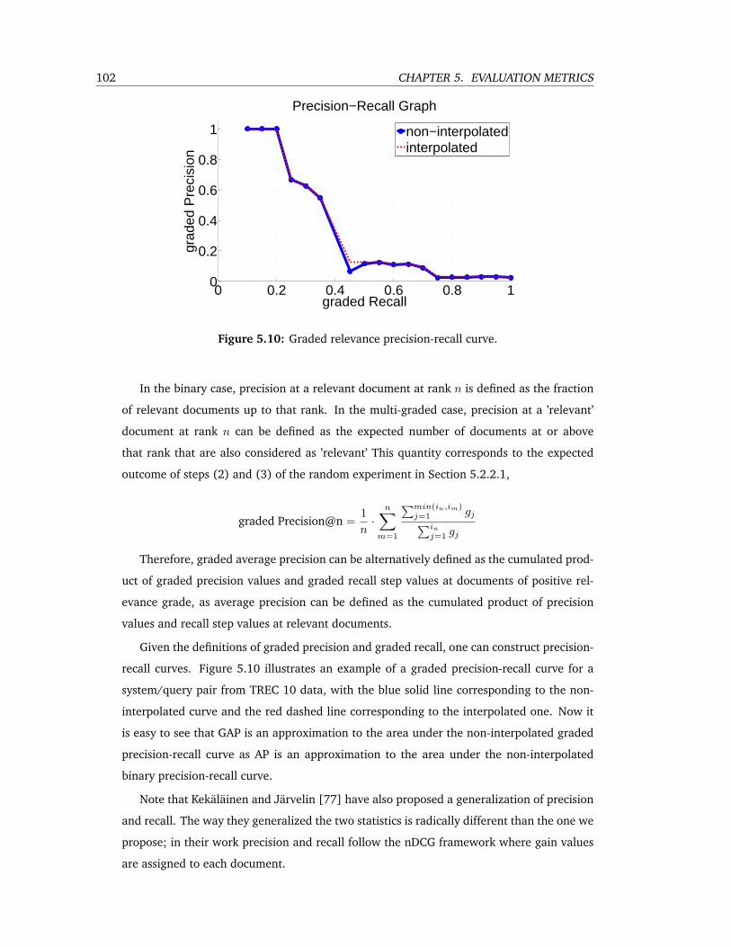
102 CHAPTER 5. EVALUATION METRICS
0 0.2 0.4 0.6 0.8 10
0.2
0.4
0.6
0.8
1
graded Recall
grad
ed P
reci
sion
Precision−Recall Graph
non−interpolatedinterpolated
Figure 5.10: Graded relevance precision-recall curve.
In the binary case, precision at a relevant document at rank n is defined as the fraction
of relevant documents up to that rank. In the multi-graded case, precision at a ’relevant’
document at rank n can be defined as the expected number of documents at or above
that rank that are also considered as ’relevant’ This quantity corresponds to the expected
outcome of steps (2) and (3) of the random experiment in Section 5.2.2.1,
graded Precision@n =1n·
n∑m=1
∑min(in,im)j=1 gj∑in
j=1 gj
Therefore, graded average precision can be alternatively defined as the cumulated prod-
uct of graded precision values and graded recall step values at documents of positive rel-
evance grade, as average precision can be defined as the cumulated product of precision
values and recall step values at relevant documents.
Given the definitions of graded precision and graded recall, one can construct precision-
recall curves. Figure 5.10 illustrates an example of a graded precision-recall curve for a
system/query pair from TREC 10 data, with the blue solid line corresponding to the non-
interpolated curve and the red dashed line corresponding to the interpolated one. Now it
is easy to see that GAP is an approximation to the area under the non-interpolated graded
precision-recall curve as AP is an approximation to the area under the non-interpolated
binary precision-recall curve.
Note that Kekalainen and Jarvelin [77] have also proposed a generalization of precision
and recall. The way they generalized the two statistics is radically different than the one we
propose; in their work precision and recall follow the nDCG framework where gain values
are assigned to each document.

5.2. EXTENSION OF AVERAGE PRECISION TO GRADED RELEVANCE JUDGMENTS 103
5.2.3 Evaluation Methodology and Results
There are two important properties that an evaluation metric should have: (1) it should
be highly informative [10] – it should summarize the quality of a search engine well, and
(2) it should be highly discriminative – it should identify the significant differences in the
performance of the systems. We evaluated GAP in terms of both of these properties. Further,
we used nDCG as a baseline for comparison purposes. Given that our goal is to propose a
good system-oriented metric that can be used as an objective function to optimize for in
LTR, in what follows we mostly focus on the informativeness of the metric since it has been
shown to correlate well with the effectiveness of the trained ranking function [149].
In particular, when a ranking function is optimized for an objective evaluation metric,
the evaluation metric used during training acts as a bottleneck that summarizes the avail-
able training data. At each training epoch, given the relevance of the documents in the
training set and the ranked list of documents retrieved by the ranking function for that
epoch, the only information the learning algorithm has access to is the value of the evalua-
tion metric. Thus, the ranking function will change on the basis of the change in the value
of the metric. Since, more informative metrics better summarize the relevance of the doc-
uments in the ranked list and thus better capture any change in the ranking of documents,
the informativeness of a metric is intuitively correlated with the ability of the LTR algorithm
to ”learn” well.
5.2.3.1 Informativeness
We use the maximum entropy framework by Aslam et al. [10] in order to analyze the infor-
mativeness of the evaluation metrics.
The maximum entropy framework is based on the assumption that the quality of a list
of documents retrieved in response to a given query is strictly a function of the relevance of
the documents retrieved within that list. The question that naturally arises is how well does
a metric capture the relevance information of the output list and consequently the effec-
tiveness of a retrieval system? In other words, given the value of a metric, for a particular
system on a particular query, how accurately can one predict the relevance of documents
retrieved by the system. In order to compute how well a metric predicts the relevance of
the returned documents, Aslam et al. [10] form a distribution over all possible sequences of
relevance and find the maximum entropy distribution over these lists given the value of the
metric. Using the maximum entropy distribution, they guarantee that they use no extra in-
formation other than the value of the given metric. Thus, using only the information given
by the metric, they form a distribution over the sequence of relevant/nonrelevant docu-
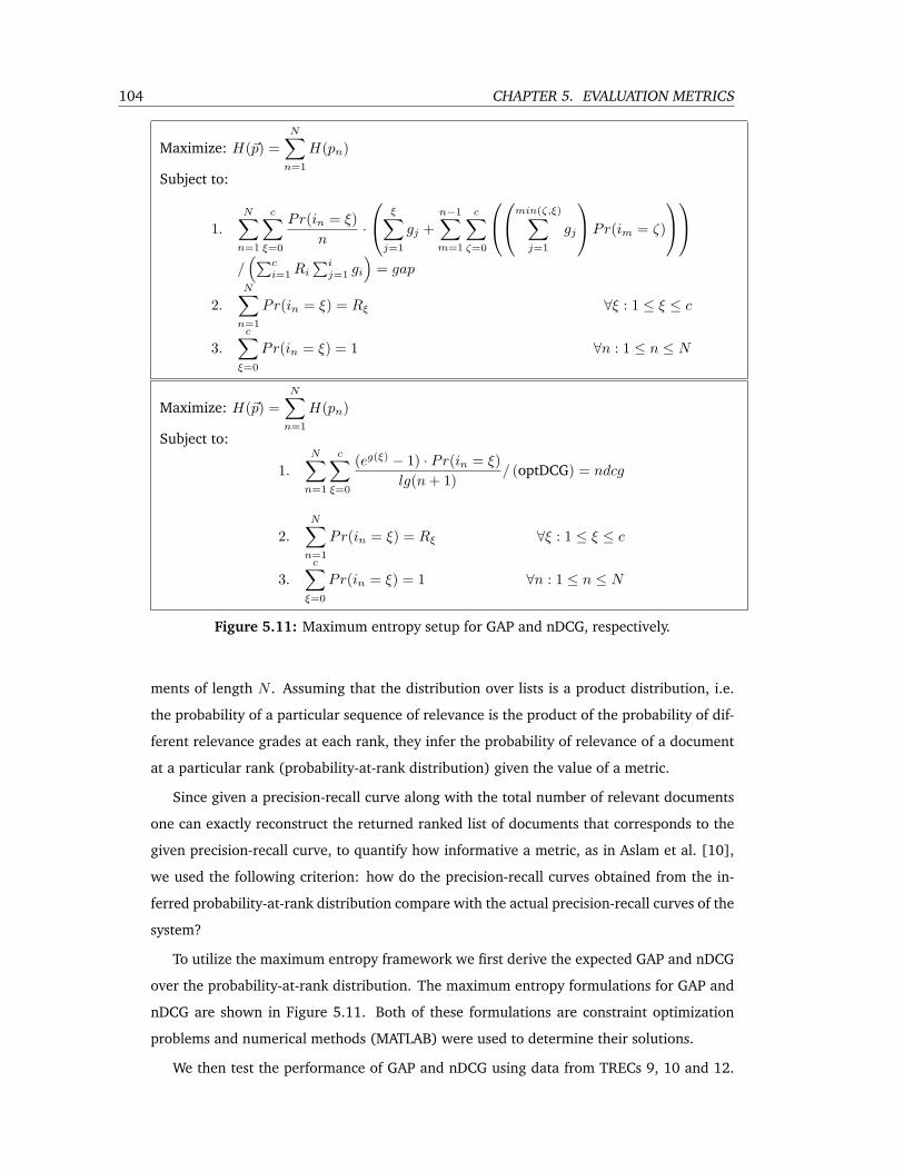
104 CHAPTER 5. EVALUATION METRICS
Maximize: H(~p) =N∑
n=1
H(pn)
Subject to:
1.N∑
n=1
c∑ξ=0
Pr(in = ξ)n
·
ξ∑j=1
gj +n−1∑m=1
c∑ζ=0
min(ζ,ξ)∑j=1
gj
Pr(im = ζ)
/
(∑ci=1 Ri
∑ij=1 gi
)= gap
2.N∑
n=1
Pr(in = ξ) = Rξ ∀ξ : 1 ≤ ξ ≤ c
3.c∑
ξ=0
Pr(in = ξ) = 1 ∀n : 1 ≤ n ≤ N
Maximize: H(~p) =N∑
n=1
H(pn)
Subject to:
1.
N∑n=1
c∑ξ=0
(eg(ξ) − 1) · Pr(in = ξ)lg(n + 1)
/ (optDCG) = ndcg
2.N∑
n=1
Pr(in = ξ) = Rξ ∀ξ : 1 ≤ ξ ≤ c
3.
c∑ξ=0
Pr(in = ξ) = 1 ∀n : 1 ≤ n ≤ N
Figure 5.11: Maximum entropy setup for GAP and nDCG, respectively.
ments of length N . Assuming that the distribution over lists is a product distribution, i.e.
the probability of a particular sequence of relevance is the product of the probability of dif-
ferent relevance grades at each rank, they infer the probability of relevance of a document
at a particular rank (probability-at-rank distribution) given the value of a metric.
Since given a precision-recall curve along with the total number of relevant documents
one can exactly reconstruct the returned ranked list of documents that corresponds to the
given precision-recall curve, to quantify how informative a metric, as in Aslam et al. [10],
we used the following criterion: how do the precision-recall curves obtained from the in-
ferred probability-at-rank distribution compare with the actual precision-recall curves of the
system?
To utilize the maximum entropy framework we first derive the expected GAP and nDCG
over the probability-at-rank distribution. The maximum entropy formulations for GAP and
nDCG are shown in Figure 5.11. Both of these formulations are constraint optimization
problems and numerical methods (MATLAB) were used to determine their solutions.
We then test the performance of GAP and nDCG using data from TRECs 9, 10 and 12.
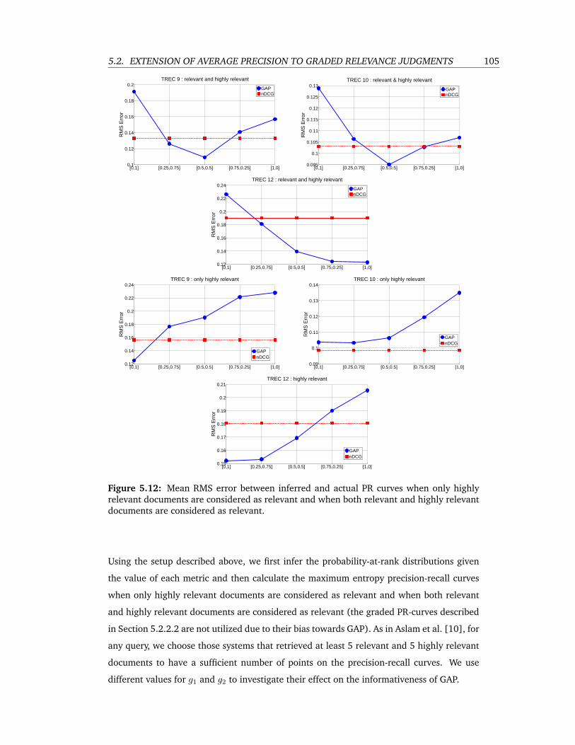
5.2. EXTENSION OF AVERAGE PRECISION TO GRADED RELEVANCE JUDGMENTS 105
[0,1] [0.25,0.75] [0.5,0.5] [0.75,0.25] [1,0]0.1
0.12
0.14
0.16
0.18
0.2
RM
S E
rror
TREC 9 : relevant and highly relevant
GAPnDCG
[0,1] [0.25,0.75] [0.5,0.5] [0.75,0.25] [1,0]0.095
0.1
0.105
0.11
0.115
0.12
0.125
0.13
RM
S E
rror
TREC 10 : relevant & highly relevant
GAPnDCG
[0,1] [0.25,0.75] [0.5,0.5] [0.75,0.25] [1,0]0.12
0.14
0.16
0.18
0.2
0.22
0.24
RM
S E
rror
TREC 12 : relevant and highly relevant
GAPnDCG
[0,1] [0.25,0.75] [0.5,0.5] [0.75,0.25] [1,0]0.12
0.14
0.16
0.18
0.2
0.22
0.24
RM
S E
rror
TREC 9 : only highly relevant
GAPnDCG
[0,1] [0.25,0.75] [0.5,0.5] [0.75,0.25] [1,0]0.09
0.1
0.11
0.12
0.13
0.14
RM
S E
rror
TREC 10 : only highly relevant
GAPnDCG
[0,1] [0.25,0.75] [0.5,0.5] [0.75,0.25] [1,0]0.15
0.16
0.17
0.18
0.19
0.2
0.21
RM
S E
rror
TREC 12 : highly relevant
GAPnDCG
Figure 5.12: Mean RMS error between inferred and actual PR curves when only highlyrelevant documents are considered as relevant and when both relevant and highly relevantdocuments are considered as relevant.
Using the setup described above, we first infer the probability-at-rank distributions given
the value of each metric and then calculate the maximum entropy precision-recall curves
when only highly relevant documents are considered as relevant and when both relevant
and highly relevant documents are considered as relevant (the graded PR-curves described
in Section 5.2.2.2 are not utilized due to their bias towards GAP). As in Aslam et al. [10], for
any query, we choose those systems that retrieved at least 5 relevant and 5 highly relevant
documents to have a sufficient number of points on the precision-recall curves. We use
different values for g1 and g2 to investigate their effect on the informativeness of GAP.
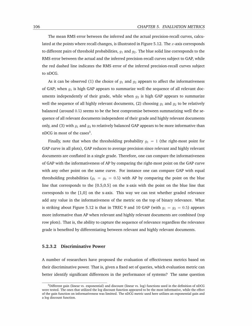
106 CHAPTER 5. EVALUATION METRICS
The mean RMS error between the inferred and the actual precision-recall curves, calcu-
lated at the points where recall changes, is illustrated in Figure 5.12. The x-axis corresponds
to different pairs of threshold probabilities, g1 and g2. The blue solid line corresponds to the
RMS error between the actual and the inferred precision-recall curves subject to GAP, while
the red dashed line indicates the RMS error of the inferred precision-recall curves subject
to nDCG.
As it can be observed (1) the choice of g1 and g2 appears to affect the informativeness
of GAP; when g1 is high GAP appears to summarize well the sequence of all relevant doc-
uments independently of their grade, while when g2 is high GAP appears to summarize
well the sequence of all highly relevant documents, (2) choosing g1 and g2 to be relatively
balanced (around 0.5) seems to be the best compromise between summarizing well the se-
quence of all relevant documents independent of their grade and highly relevant documents
only, and (3) with g1 and g2 to relatively balanced GAP appears to be more informative than
nDCG in most of the cases3.
Finally, note that when the thresholding probability g1 = 1 (the right-most point for
GAP curve in all plots), GAP reduces to average precision since relevant and highly relevant
documents are conflated in a single grade. Therefore, one can compare the informativeness
of GAP with the informativeness of AP by comparing the right-most point on the GAP curve
with any other point on the same curve. For instance one can compare GAP with equal
thresholding probabilities (g1 = g2 = 0.5) with AP by comparing the point on the blue
line that corresponds to the [0.5,0.5] on the x-axis with the point on the blue line that
corresponds to the [1,0] on the x-axis. This way we can test whether graded relevance
add any value in the informativeness of the metric on the top of binary relevance. What
is striking about Figure 5.12 is that in TREC 9 and 10 GAP (with g1 = g2 = 0.5) appears
more informative than AP when relevant and highly relevant documents are combined (top
row plots). That is, the ability to capture the sequence of relevance regardless the relevance
grade is benefited by differentiating between relevant and highly relevant documents.
5.2.3.2 Discriminative Power
A number of researchers have proposed the evaluation of effectiveness metrics based on
their discriminative power. That is, given a fixed set of queries, which evaluation metric can
better identify significant differences in the performance of systems? The same question
3Different gain (linear vs. exponential) and discount (linear vs. log) functions used in the definition of nDCGwere tested. The ones that utilized the log discount function appeared to be the most informative, while the effectof the gain function on informativeness was limitted. The nDCG metric used here utilizes an exponential gain anda log discount function.
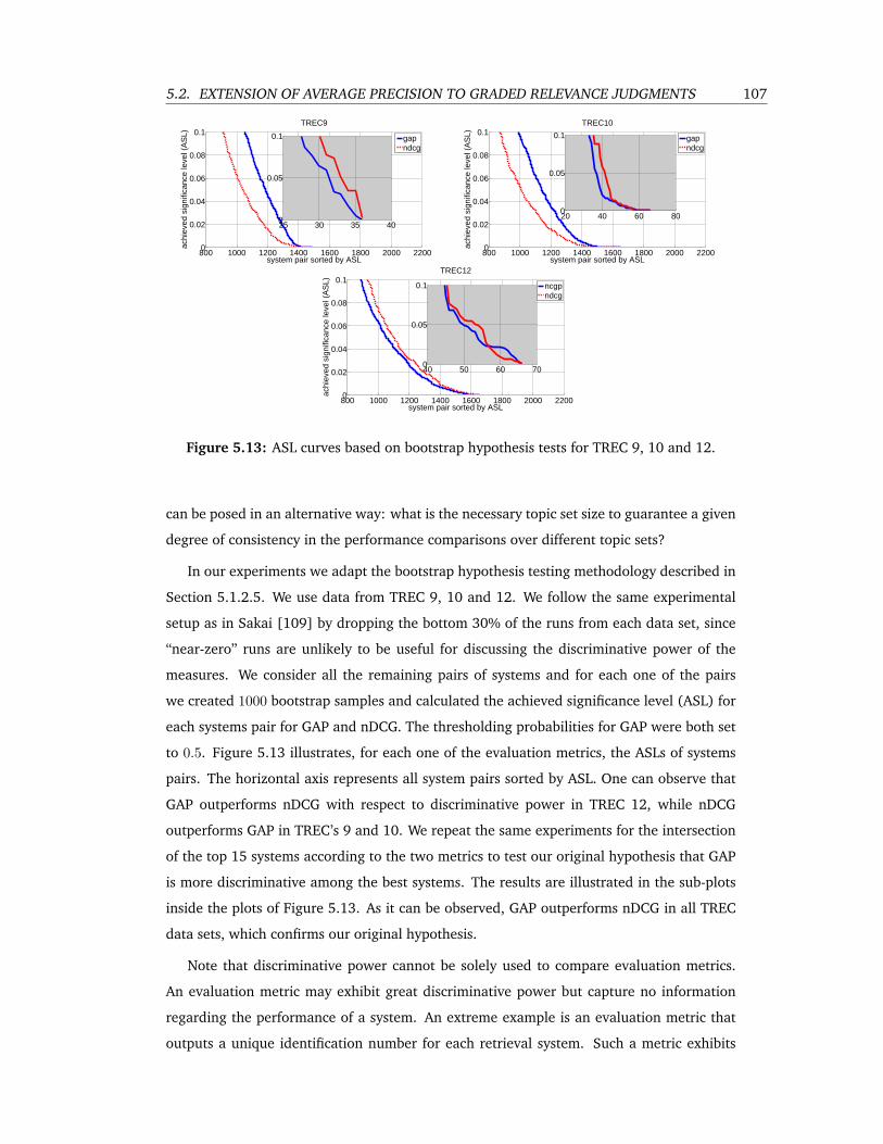
5.2. EXTENSION OF AVERAGE PRECISION TO GRADED RELEVANCE JUDGMENTS 107
800 1000 1200 1400 1600 1800 2000 22000
0.02
0.04
0.06
0.08
0.1
system pair sorted by ASL
achi
eved
sig
nific
ance
leve
l (A
SL)
TREC9
gapndcg
25 30 35 400
0.05
0.1
800 1000 1200 1400 1600 1800 2000 22000
0.02
0.04
0.06
0.08
0.1
system pair sorted by ASL
achi
eved
sig
nific
ance
leve
l (A
SL)
TREC10
gapndcg
20 40 60 800
0.05
0.1
800 1000 1200 1400 1600 1800 2000 22000
0.02
0.04
0.06
0.08
0.1
system pair sorted by ASL
achi
eved
sig
nific
ance
leve
l (A
SL)
TREC12
ncgpndcg
40 50 60 700
0.05
0.1
Figure 5.13: ASL curves based on bootstrap hypothesis tests for TREC 9, 10 and 12.
can be posed in an alternative way: what is the necessary topic set size to guarantee a given
degree of consistency in the performance comparisons over different topic sets?
In our experiments we adapt the bootstrap hypothesis testing methodology described in
Section 5.1.2.5. We use data from TREC 9, 10 and 12. We follow the same experimental
setup as in Sakai [109] by dropping the bottom 30% of the runs from each data set, since
“near-zero” runs are unlikely to be useful for discussing the discriminative power of the
measures. We consider all the remaining pairs of systems and for each one of the pairs
we created 1000 bootstrap samples and calculated the achieved significance level (ASL) for
each systems pair for GAP and nDCG. The thresholding probabilities for GAP were both set
to 0.5. Figure 5.13 illustrates, for each one of the evaluation metrics, the ASLs of systems
pairs. The horizontal axis represents all system pairs sorted by ASL. One can observe that
GAP outperforms nDCG with respect to discriminative power in TREC 12, while nDCG
outperforms GAP in TREC’s 9 and 10. We repeat the same experiments for the intersection
of the top 15 systems according to the two metrics to test our original hypothesis that GAP
is more discriminative among the best systems. The results are illustrated in the sub-plots
inside the plots of Figure 5.13. As it can be observed, GAP outperforms nDCG in all TREC
data sets, which confirms our original hypothesis.
Note that discriminative power cannot be solely used to compare evaluation metrics.
An evaluation metric may exhibit great discriminative power but capture no information
regarding the performance of a system. An extreme example is an evaluation metric that
outputs a unique identification number for each retrieval system. Such a metric exhibits
108 CHAPTER 5. EVALUATION METRICS
absolute discriminative power, but captures no information regarding the quality of the
retrieval system.
5.2.4 GAP for Learning to Rank
Finally, we employed GAP as an objective function to optimize for in the context of LTR. For
comparison purposes we also optimized for AP and nDCG. In our experiments we employed
two different learning algorithms, (a) SoftRank [129] and (b) LambdaRank [27] over two
different data sets, (a) a Web collection with 5K queries and 382 features taken from a
commercial search engine, and (b) the OHSUMED collection provided by LETOR [128]. The
relevance judgments in the both data set are in a 3 grade scale (non-relevant, relevant and
highly relevant). Five-fold cross validation was used in the case of OHSUMED collection.
Since the informativeness of the metric is well correlated with the effectiveness of the
constructed ranking function, we select g1 and g2 based on the criterion of informativeness.
As we observed in Section 5.2.3.1, the values of gi that result in the most informative GAP
variation is g1 = g2 = 0.5. Intuitively, these values of gi indicate that highly relevant
documents are ”twice as important as relevant documents.
LTR algorithms: SoftRank [129] is a neural network based algorithm that is designed
to directly optimize for nDCG, as most other learning to rank algorithms. Since most IR
metrics are non-smooth as as they depend on the ranks of documents, the main idea used
in SoftRank to overcome the problem of optimizing non-smooth IR metrics is based on
defining smooth versions of information retrieval metrics by assuming that the score sj of
each document j is a value generated according to a Gaussian distribution with mean equal
to sj and shared smoothing variance σs. Based on this, Taylor et al. [129] define πij as
the probability that document i will be ranked higher than document j. This distribution
can then be used to define smooth versions of IR metrics as expectations over these rank
distributions.
Based on these definitions, we extend SoftRank to optimize for GAP by defining Soft-
GAP, the expected value of Graded Average Precision with respect to these distributions and
compute the gradient of SoftGAP.
Given the probabilistic interpretation of GAP defined earlier and the distribution πij ,
the probability that document i will be ranked higher than document j, SoftGAP can be
computed as follows:
Let PCn be:
PCn =
∑in
j=1 gj +∑N
m=1 πmn
∑min(im,in)j=1 gj∑N
m=1,m 6=n πmn + 1
then,
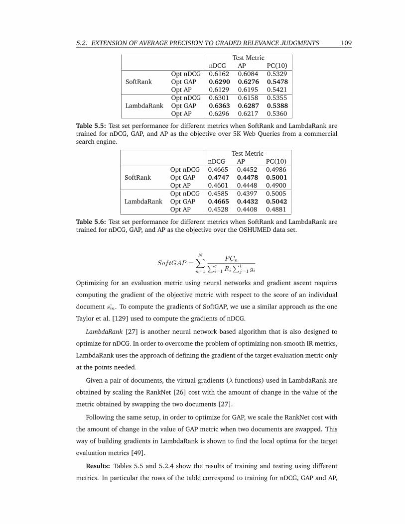
5.2. EXTENSION OF AVERAGE PRECISION TO GRADED RELEVANCE JUDGMENTS 109
Test MetricnDCG AP PC(10)
SoftRankOpt nDCG 0.6162 0.6084 0.5329Opt GAP 0.6290 0.6276 0.5478Opt AP 0.6129 0.6195 0.5421
LambdaRankOpt nDCG 0.6301 0.6158 0.5355Opt GAP 0.6363 0.6287 0.5388Opt AP 0.6296 0.6217 0.5360
Table 5.5: Test set performance for different metrics when SoftRank and LambdaRank aretrained for nDCG, GAP, and AP as the objective over 5K Web Queries from a commercialsearch engine.
Test MetricnDCG AP PC(10)
SoftRankOpt nDCG 0.4665 0.4452 0.4986Opt GAP 0.4747 0.4478 0.5001Opt AP 0.4601 0.4448 0.4900
LambdaRankOpt nDCG 0.4585 0.4397 0.5005Opt GAP 0.4665 0.4432 0.5042Opt AP 0.4528 0.4408 0.4881
Table 5.6: Test set performance for different metrics when SoftRank and LambdaRank aretrained for nDCG, GAP, and AP as the objective over the OSHUMED data set.
SoftGAP =N∑
n=1
PCn∑ci=1 Ri
∑ij=1 gi
Optimizing for an evaluation metric using neural networks and gradient ascent requires
computing the gradient of the objective metric with respect to the score of an individual
document sm. To compute the gradients of SoftGAP, we use a similar approach as the one
Taylor et al. [129] used to compute the gradients of nDCG.
LambdaRank [27] is another neural network based algorithm that is also designed to
optimize for nDCG. In order to overcome the problem of optimizing non-smooth IR metrics,
LambdaRank uses the approach of defining the gradient of the target evaluation metric only
at the points needed.
Given a pair of documents, the virtual gradients (λ functions) used in LambdaRank are
obtained by scaling the RankNet [26] cost with the amount of change in the value of the
metric obtained by swapping the two documents [27].
Following the same setup, in order to optimize for GAP, we scale the RankNet cost with
the amount of change in the value of GAP metric when two documents are swapped. This
way of building gradients in LambdaRank is shown to find the local optima for the target
evaluation metrics [49].
Results: Tables 5.5 and 5.2.4 show the results of training and testing using different
metrics. In particular the rows of the table correspond to training for nDCG, GAP and AP,
110 CHAPTER 5. EVALUATION METRICS
respectively. The columns correspond to testing for nDCG at cutoff 3, 5 and 10, AP and
precision at cutoff 10. As it can be observed in the table training for GAP outperforms both
training for nDCG and AP, even if the test metric is nDCG or AP respectively. The differ-
ences among the effectiveness of the resulting ranking functions are not large, however,
(1) most of them are statistically significant, indicating that the fact that GAP outperforms
AP and nDCG is not a results of any random noise in training data, (2) GAP consistently
leads to the best performing ranking function over two radically different data sets, and
(3) GAP consistently leads to the best performing ranking function over two different LTR
algorithms. Thus, even if the differences among the constructed ranking functions are not
large, optimizing for GAP can only lead to better ranking functions.
These results strengthen the conclusion drawn from the discussion about the informa-
tiveness of the metrics. First, it can be clearly seen that even in the case that we care about
a binary measure (AP or PC at 10) the utilization of multi-graded relevance judgments is
highly beneficial. Furthermore, these results suggest that even if one cares for nDCG at
early ranks, one should still train for GAP as opposed to training for nDCG.
5.2.5 Conclusions
We constructed a new metric of retrieval effectiveness (GAP) in a systematic manner that
directly generalizes average precision to the multi-graded relevance case. As such, it inherits
all desirable properties of AP: it has a nice probabilistic interpretation and a theoretical
foundation; it estimates the area under the non-interpolated grade precision-recall curve.
Furthermore, the new metric is highly informative and highly discriminative. Finally, when
used as an objective function for learning-to-rank purposes GAP consistently outperforms
AP and nDCG over two different data sets and over three different learning algorithms even
when the test metric is AP or nDCG itself.
5.3 Overall Conclusions
Evaluation metrics are employed both to summarize the effectiveness of a retrieval system
and as objective functions to be optimized in learning-to-rank. Traditional evaluation met-
rics, such as average precision, even though they are very popular, assume that documents
are either relevant or nonrelevant to a user’s information request ignoring the fact that nat-
urally some documents are more relevant than others. Consequently, in evaluation they do
not capture all available information about the effectiveness of a system and in learning-to-
rank they ignore swaps between documents of different relevance grade and thus they do
not guide the training of new ranking functions in the most optimal manner.
5.3. OVERALL CONCLUSIONS 111
The nDCG metric has proven to be one of the most popular multi-graded relevance
metric, however defining the appropriate gain and discount function with respect to user
satisfaction is a hard problem. In this work, instead we proposed a methodological way
of defining the gain and the discount function of nDCG by optimizing the efficiency of the
metric, that is by minimizing the number of queries required to reliably discriminate a good
from a bad systems. Different gain and discount functions however may lead to nDCG
variants that evaluate different aspects of a system’s retrieval effectiveness and since the
choice of gain and discount functions appear to be dependent on the data collection and
the participating systems, this could lead to inconsistencies in the evaluation over different
collections. To overcome the difficulties and uncertainties regarding the choice of gain
and discount functions for nDCG, we proposed an extension of average precision to multi-
graded relevance judgments. The new metric, GAP, has a nice probabilistic interpretation
and a theoretical foundation. Further it is highly informative and discriminative. Finally, we
compared GAP with nDCG when used as objective function for learning-to-rank purposes
and GAP clearly outperforms nDCG even when the test metric is nDCG itself.

CHAPTER 6
Conclusions
In this work we have considered the construction of reliable and efficient test and training
collections to be used in the evaluation of retrieval systems and in the development of new
and effective ranking functions. In the process of building such collections we investigated
methods of selecting the appropriate documents and queries to be judged and we proposed
evaluation metrics that better capture the overall effectiveness of the retrieval systems under
study.
In particular, we demonstrated that low-cost evaluation, by carefully selecting docu-
ments per query to be judged and also queries to be included in the test collections, can
lead to effective and reliable evaluation. By utilizing our evaluation methodology IR re-
searchers and engineers can construct new and customized test collections with minimal
cost to test new ideas, while customers can easily compare different retrieval system op-
tions and select the one that best fits their needs. Furthermore, with the same budget as
the one currently used by multinational corporations and governmental organizations like
NIST, we have shown that larger and thus more diverse and more representative and at the
same time more reliable test collections can be constructed. Our work on query selection
is a preliminary step towards this direction and more work is needed to methodologically
understand and decide what queries are better to evaluate on. Therefore, we plan to carry
on this line of research, (a) in a top-down approach by examining different query categories
and whether some query categories are more useful than others (e.g. in Million Query at
TREC 2009 we plan to examine what distribution over query hardness and query intent can
lead to more effective and efficient evaluation), and (b) in a bottom-up approach through
item-response analysis that can reveal how well a single query or a set of queries can dis-
criminate different systems.
Further, we illustrated that the construction of training collections needs to be carefully
studied. Specifically, we showed that the way documents are selected to be included in
training collections affect the effectiveness of the constructed ranking functions. Some pre-
liminary results of on-going research has also shown that queries in training collections also
113
114 CHAPTER 6. CONCLUSIONS
affect the effectiveness of the obtained ranking functions. Even though the construction of
training collections faces similar issues with the construction of test collections the solutions
are not necessary the same and thus using test collections for the purpose of learning-to-
rank may not be the optimal way to construct new ranking functions. In learning-to-rank a
large number of factors and especially their interactions may affect the effectiveness of the
final ranking function. In particular we have shown preliminary results on the interactions
between the machine learning algorithm used and the document selection methodology
with some algorithms being more robust than others both regarding the incompleteness
of the constructed training collection and the methodology to select those documents. We
plan to continue investigating different factors that affect the effectiveness of the ranking
functions along with their interactions.
Finally, we have shown that evaluation metrics also affect both the effectiveness of the
evaluation and the effectiveness of learning-to-rank. We plan to continue investigating the
effectiveness of different evaluation metrics following two different directions: (a) for the
purpose of evaluation we plan to move towards evaluation metrics that better associate
with user satisfaction by utilizing tools like Amazon’s Mechanical Turk that can be used
to provide inexpensive judgments and query logs that provide useful information about
users’ interactions with the retrieval system, and (b) for the purpose of learning-to-rank
we plan to continue our work on metrics of overall effectiveness even though they may
not best correlate with user satisfaction. In particular, we intent to investigate how newly
proposed metrics that can effectively evaluate new IR tasks, such as novelty retrieval, can
be optimized to result in ranking functions that best fulfill users’ need, e.g. by diversifying
the ranked list of documents returned to the user.
Bibliography
[1] Azzah Al-Maskari, Mark Sanderson, and Paul Clough. The relationship between IR
effectiveness measures and user satisfaction. In SIGIR ’07: Proceedings of the 30th an-
nual international ACM SIGIR conference on Research and development in information
retrieval, pages 773–774, New York, NY, USA, 2007. ACM.
[2] Azzah Al-Maskari, Mark Sanderson, and Paul Clough. Relevance judgments between
TREC and non-TREC assessors. In SIGIR ’08: Proceedings of the 31st annual inter-
national ACM SIGIR conference on Research and development in information retrieval,
pages 683–684, New York, NY, USA, 2008. ACM.
[3] James Allan, Ben Carterette, Javed A. Aslam, Virgil Pavlu, Blagovest Dachev, and
Evangelos Kanoulas. Million query track 2007 overview. In Ellen M. Voorhees and
Lori P. Buckland, editors, The Sixteenth Text REtrieval Conference Proceedings (TREC
2007). National Institute of Standards and Technology, December 2008. NIST Spe-
cial Publication SP 500-274.
[4] James Allan, Ben Carterette, Javed A. Aslam, Virgil Pavlu, and Evangelos Kanoulas.
Million query track 2008 overview. In Ellen M. Voorhees and Lori P. Buckland, ed-
itors, The Seventeenth Text REtrieval Conference Proceedings (TREC 2008). National
Institute of Standards and Technology, December 2009. To appear.
[5] Javed A. Aslam, Virgil Pavlu, and Emine Yilmaz. A statistical method for system eval-
uation using incomplete judgments. In Susan Dumais, Efthimis N. Efthimiadis, David
Hawking, and Kalervo Jarvelin, editors, Proceedings of the 29th Annual International
ACM SIGIR Conference on Research and Development in Information Retrieval, pages
541–548. ACM Press, August 2006.
[6] Javed A. Aslam, Virgiliu Pavlu, and Robert Savell. A unified model for metasearch
and the efficient evaluation of retrieval systems via the hedge algorithm. In Jamie
Callan, Gordon Cormack, Charles Clarke, David Hawking, and Alan Smeaton, edi-
115
116 BIBLIOGRAPHY
tors, Proceedings of the 26th Annual International ACM SIGIR Conference on Research
and Development in Information Retrieval, pages 393–394. ACM Press, July 2003.
[7] Javed A. Aslam and Robert Savell. On the effectiveness of evaluating retrieval sys-
tems in the absence of relevance judgments. In Jamie Callan, Gordon Cormack,
Charles Clarke, David Hawking, and Alan Smeaton, editors, Proceedings of the 26th
Annual International ACM SIGIR Conference on Research and Development in Informa-
tion Retrieval, pages 361–362. ACM Press, July 2003.
[8] Javed A. Aslam and Emine Yilmaz. A geometric interpretation and analysis of R-
precision. In Proceedings of the Fourteenth ACM International Conference on Informa-
tion and Knowledge Management, pages 664–671. ACM Press, October 2005.
[9] Javed A. Aslam, Emine Yilmaz, and Virgiliu Pavlu. A geometric interpretation of R-
precision and its correlation with average precision. In Gary Marchionini, Alistair
Moffat, John Tait, Ricardo Baeza-Yates, and Novio Ziviani, editors, Proceedings of
the 28th Annual International ACM SIGIR Conference on Research and Development in
Information Retrieval, pages 573–574. ACM Press, August 2005.
[10] Javed A. Aslam, Emine Yilmaz, and Virgiliu Pavlu. The maximum entropy method for
analyzing retrieval measures. In Gary Marchionini, Alistair Moffat, John Tait, Ricardo
Baeza-Yates, and Novio Ziviani, editors, Proceedings of the 28th Annual International
ACM SIGIR Conference on Research and Development in Information Retrieval, pages
27–34. ACM Press, August 2005.
[11] Ricardo Baeza-Yates and Berthier Ribeiro-Neto. Modern Information Retrieval. ACM
Press, 1999.
[12] P. Bailey, N. Craswell, A. P. de Vries, I. Soboroff, and P. Thomas. Overview of the
TREC 2008 enterprise track. In Proceedings of the Seventeenth Text REtrieval Confer-
ence (TREC 2008), 2008.
[13] Peter Bailey, Nick Craswell, Ian Soboroff, Paul Thomas, Arjen P. de Vries, and Emine
Yilmaz. Relevance assessment: are judges exchangeable and does it matter. In SIGIR
’08: Proceedings of the 31st annual international ACM SIGIR conference on Research
and development in information retrieval, pages 667–674, New York, NY, USA, 2008.
ACM.
[14] David Banks, Paul Over, and Nien-Fan Zhang. Blind men and elephants: Six ap-
proaches to TREC data. Inf. Retr., 1(1-2):7–34, 1999.
117
[15] Steven M. Beitzel, Eric C. Jensen, Abdur Chowdhury, David Grossman, and Ophir
Frieder. Using manually-built web directories for automatic evaluation of known-
item retrieval. In SIGIR ’03: Proceedings of the 26th annual international ACM SIGIR
conference on Research and development in informaion retrieval, pages 373–374, New
York, NY, USA, 2003. ACM.
[16] Adam Berger and John Lafferty. Information retrieval as statistical translation. In
SIGIR ’99: Proceedings of the 22nd annual international ACM SIGIR conference on
Research and development in information retrieval, pages 222–229, New York, NY,
USA, 1999. ACM.
[17] David Bodoff and Pu Li. Test theory for assessing IR test collection. In Proceedings of
SIGIR, pages 367–374, 2007.
[18] Tanuja Bompada, Chi-Chao Chang, John Chen, Ravi Kumar, and Rajesh Shenoy. On
the robustness of relevance measures with incomplete judgments. In SIGIR ’07: Pro-
ceedings of the 30th annual international ACM SIGIR conference on Research and de-
velopment in information retrieval, pages 359–366, New York, NY, USA, 2007. ACM
Press.
[19] Martin Braschler and Carol Peters. Cross-language evaluation forum: Objectives,
results, achievements. Information Retrieval, 7(1):7–31, 2004.
[20] Robert L. Brennan. Generalizability Theory. Springer-Verlag, New York, 2001.
[21] K. R. W. Brewer and M Hanif. Sampling With Unequal Probabilities. Springer, New
York, 1983.
[22] Chris Buckley, Darrin Dimmick, Ian Soboroff, and Ellen Voorhees. Bias and the limits
of pooling. In SIGIR ’06: Proceedings of the 29th annual international ACM SIGIR
conference on Research and development in information retrieval, pages 619–620, New
York, NY, USA, 2006. ACM.
[23] Chris Buckley and Stephen E. Robertson. Relevance feedback track overview. In
Proceedings of the Seventeenth Text REtrieval Conference (TREC 2008), 2008.
[24] Chris Buckley and Ellen M. Voorhees. Evaluating evaluation measure stability. In
Proceedings of the 23rd Annual International ACM SIGIR Conference on Research and
Development in Information Retrieval, pages 33–40, 2000.
[25] Chris Buckley and Ellen M. Voorhees. Retrieval evaluation with incomplete infor-
mation. In Proceedings of the 27th Annual International ACM SIGIR Conference on
Research and Development in Information Retrieval, pages 25–32, 2004.
118 BIBLIOGRAPHY
[26] Chris Burges, Tal Shaked, Erin Renshaw, Ari Lazier, Matt Deeds, Nicole Hamilton,
and Greg Hullender. Learning to rank using gradient descent. In ICML ’05: Pro-
ceedings of the 22nd international conference on Machine learning, pages 89–96, New
York, NY, USA, 2005. ACM Press.
[27] Christopher J. C. Burges, Robert Ragno, and Quoc V. Le. Learning to rank with
nonsmooth cost functions. In Bernhard Scholkopf, John C. Platt, Thomas Hoffman,
Bernhard Scholkopf, John C. Platt, and Thomas Hoffman, editors, NIPS, pages 193–
200. MIT Press, 2006.
[28] Stefan Buttcher, Charles Clarke, and Ian Soboroff. The TREC 2006 terabyte track. In
Proceedings of the Fifteenth Text REtrieval Conference (TREC 2006), 2006.
[29] Zhe Cao, Tao Qin, Tie-Yan Liu, Ming-Feng Tsai, and Hang Li. Learning to rank:
from pairwise approach to listwise approach. In ICML ’07: Proceedings of the 24th
international conference on Machine learning, pages 129–136, New York, NY, USA,
2007. ACM.
[30] Ben Carterette. Robust test collections for retrieval evaluation. In Proceedings of
SIGIR, pages 55–62, 2007.
[31] Ben Carterette and James Allan. Incremental test collections. In CIKM ’05: Proceed-
ings of the 14th ACM international conference on Information and knowledge manage-
ment, pages 680–687, New York, NY, USA, 2005. ACM Press.
[32] Ben Carterette, James Allan, and Ramesh Sitaraman. Minimal test collections for
retrieval evaluation. In Proceedings of the 29th Annual International ACM SIGIR Con-
ference on Research and Development in Information Retrieval, pages 268–275, 2006.
[33] Ben Carterette, Virgil Pavlu, Evangelos Kanoulas, Javed A. Aslam, and James Allan.
Evaluation over thousands of queries. In Sung-Hyon Myaeng, Douglas W. Oard, Fab-
rizio Sebastiani, Tat-Seng Chua, and Mun-Kew Leong, editors, Proceedings of the 31st
Annual International ACM SIGIR Conference on Research and Development in Informa-
tion Retrieval, pages 651–658. ACM Press, July 2008.
[34] Matteo Cattelan and Stefano Mizzaro. IR evaluation without a common set of topics.
In ICTIR, pages 342–345, 2009.
[35] Soumen Chakrabarti, Martin van den Berg, and Byron Dom. Focused crawling: a
new approach to topic-specific web resource discovery. Computer Networks, 31(11-
16):1623–1640, 1999.
119
[36] Olivier Chapelle, Donald Metlzer, Ya Zhang, and Pierre Grinspan. Expected recip-
rocal rank for graded relevance. In In Proceedings of the 18th ACM Conference on
Information and Knowledge Management (CIKM), 2009.
[37] Stanley F. Chen and Joshua Goodman. An empirical study of smoothing techniques
for language modeling. In Proceedings of the Thirty-Fourth Annual Meeting of the
Association for Computational Linguistics, pages 310–318, 1996.
[38] Junghoo Cho, Hector Garcia-Molina, and Lawrence Page. Efficient crawling through
url ordering. Comput. Netw. ISDN Syst., 30(1-7):161–172, 1998.
[39] Charles Clarke, Nick Craswell, and Ian Soboroff. Overview of the TREC 2004 Ter-
abyte Track. In Proceedings of TREC, 2004.
[40] Cyril Cleverdon. The cranfield tests on index language devices. In Readings in infor-
mation retrieval, pages 47–59. Morgan Kaufmann Publishers Inc., San Francisco, CA,
USA, 1997.
[41] Cyril W. Cleverdon. The significance of the cranfield tests on index languages. In
SIGIR ’91: Proceedings of the 14th annual international ACM SIGIR conference on
Research and development in information retrieval, pages 3–12, New York, NY, USA,
1991. ACM.
[42] William S. Cooper. Expected search length: a single measure of retrieval effectiveness
based on the weak ordering action of retrieval systems. American Documentation,
19:30–41, 1968.
[43] William S. Cooper. On selecting a measure of retrieval effectiveness. Part I. Readings
in Information Retrieval, pages 191–204, 1997.
[44] Gordon V. Cormack, Christopher R. Palmer, and Charles L. A. Clarke. Efficient con-
struction of large test collections. In W. Bruce Croft, Alistair Moffat, C. J. van Ri-
jsbergen, Ross Wilkinson, and Justin Zobel, editors, Proceedings of the 21th Annual
International ACM SIGIR Conference on Research and Development in Information Re-
trieval, pages 282–289, August 1998.
[45] Nick Craswell, Onno Zoeter, Michael Taylor, and Bill Ramsey. An experimental com-
parison of click position-bias models. In WSDM ’08: Proceedings of the international
conference on Web search and web data mining, pages 87–94, New York, NY, USA,
2008. ACM.
120 BIBLIOGRAPHY
[46] Bruce Croft, Donald Metzler, and Trevor Strohman. Search Engines: Information
Retrieval in Practice. Addison Wesley, February 2009.
[47] W. Bruce Croft and John Lafferty. Language Modeling for Information Retrieval.
Kluwer Academic Publishers, Norwell, MA, USA, 2003.
[48] B. Dervin and M. S. Nilan. Information needs and use. In Annual Review of Informa-
tion Science and Technology, volume 21, pages 3–33, 1986.
[49] Pinar Donmez, Krysta M. Svore, and Christopher J.C. Burges. On the local optimality
of lambdarank. In SIGIR ’09: Proceedings of the 32nd international ACM SIGIR confer-
ence on Research and development in information retrieval, pages 460–467, New York,
NY, USA, 2009. ACM.
[50] Miles Efron. Using multiple query aspects to build test collections without human
relevance judgments. In ECIR, pages 276–287, 2009.
[51] Ronald Fagin, Ravi Kumar, Kevin S. McCurley, Jasmine Novak, D. Sivakumar, John A.
Tomlin, and David P. Williamson. Searching the workplace web. In WWW ’03:
Proceedings of the 12th international conference on World Wide Web, pages 366–375,
New York, NY, USA, 2003. ACM.
[52] Dennis Fetterly, Nick Craswell, and Vishwa Vinay. Measuring the search effectiveness
of a breadth-first crawl. In ECIR ’09: Proceedings of the 31th European Conference on
IR Research on Advances in Information Retrieval, pages 388–399, Berlin, Heidelberg,
2009. Springer-Verlag.
[53] Yoav Freund, Raj Iyer, Robert E. Schapire, and Yoram Singer. An efficient boosting
algorithm for combining preferences. J. Mach. Learn. Res., 4:933–969, 2003.
[54] Yoav Freund, Raj Iyer, Robert E. Schapire, Yoram Singer, and G. Dietterich. An effi-
cient boosting algorithm for combining preferences. In Journal of Machine Learning
Research, pages 170–178. Morgan Kaufmann, 1998.
[55] Norbert Fuhr, Norbert Govert, Gabriella Kazai, and Mounia Lalmas, editors. Proceed-
ings of the First Workshop of the INitiative for the Evaluation of XML Retrieval (INEX),
Schloss Dagstuhl, Germany, December 9-11, 2002, 2002.
[56] Glenn Fung, Romer Rosales, and Balaji Krishnapuram. Learning rankings via convex
hull separation. In In Advances in Neural Information Processing Systems 18, pages
395–402. MIT Press, 2006.
121
[57] Jianfeng Gao, Jian-Yun Nie, Guangyuan Wu, and Guihong Cao. Dependence lan-
guage model for information retrieval. In SIGIR ’04: Proceedings of the 27th annual
international ACM SIGIR conference on Research and development in information re-
trieval, pages 170–177, New York, NY, USA, 2004. ACM.
[58] Erik Graf and Leif Azzopardi. A methodology for building a patent test collection
for prior art search. In The Second International Workshop on Evaluating Information
Access (EVIA), December 16, 2008, Tokyo, Japan, pages 60–71, 2008.
[59] Zoltan Gyongyi, Hector Garcia-Molina, and Jan Pedersen. Combating web spam with
trustrank. In VLDB ’04: Proceedings of the Thirtieth international conference on Very
large data bases, pages 576–587. VLDB Endowment, 2004.
[60] Donna Harman. Overview of the Third Text REtreival conference (TREC-3). In
Proceedings of the Fifth Text REtrieval Conference (TREC-3), pages 1–19, 1995.
[61] Donna Harman. Overview of the Fourth Text REtrieval Conference (TREC-4). In
Donna Harman, editor, Proceedings of the Fourth Text REtrieval Conference (TREC-4),
pages 1–23, October 1996. NIST Special Publication 500-236.
[62] David Hawking. Challenges in enterprise search. In ADC ’04: Proceedings of the
15th Australasian database conference, pages 15–24, Darlinghurst, Australia, Aus-
tralia, 2004. Australian Computer Society, Inc.
[63] David Hawking and Nick Craswell. Overview of the TREC 2001 Web track. In
Proceedings of TREC, pages 61–67, 2001.
[64] David Hawking and Stephen Robertson. On collection size and retrieval effective-
ness. Inf. Retr., 6(1):99–105, 2003.
[65] Djoerd Hiemstra. A linguistically motivated probabilistic model of information re-
trieval. In ECDL ’98: Proceedings of the Second European Conference on Research
and Advanced Technology for Digital Libraries, pages 569–584, London, UK, 1998.
Springer-Verlag.
[66] Yunhua Hu, Guomao Xin, Ruihua Song, Guoping Hu, Shuming Shi, Yunbo Cao, and
Hang Li. Title extraction from bodies of html documents and its application to web
page retrieval. In SIGIR ’05: Proceedings of the 28th annual international ACM SIGIR
conference on Research and development in information retrieval, pages 250–257, New
York, NY, USA, 2005. ACM.
122 BIBLIOGRAPHY
[67] David A. Hull. Using statistical testing in the evaluation of retrieval experiments. In
Research and Development in Information Retrieval, pages 329–338, 1993.
[68] Kalervo Jarvelin and Jaana Kekalainen. IR evaluation methods for retrieving highly
relevant documents. In SIGIR ’00: Proceedings of the 23rd annual international ACM
SIGIR conference on Research and development in information retrieval, pages 41–48,
New York, NY, USA, 2000. ACM Press.
[69] Kalervo Jarvelin and Jaana Kekalainen. Cumulated gain-based evaluation of IR tech-
niques. ACM Transactions on Information Systems, 20(4):422–446, 2002.
[70] T. Joachims. Training linear SVMs in linear time. In ACM SIGKDD International
Conference On Knowledge Discovery and Data Mining (KDD), pages 217–226, 2006.
[71] Thorsten Joachims. Estimating the generalization performance of a SVM efficiently.
In Pat Langley, editor, Proceedings of ICML-00, 17th International Conference on Ma-
chine Learning, pages 431–438, Stanford, US, 2000. Morgan Kaufmann Publishers,
San Francisco, US.
[72] Thorsten Joachims, Laura Granka, Bing Pan, Helene Hembrooke, and Geri Gay. Ac-
curately interpreting clickthrough data as implicit feedback. In SIGIR ’05: Proceedings
of the 28th annual international ACM SIGIR conference on Research and development
in information retrieval, pages 154–161, New York, NY, USA, 2005. ACM.
[73] K. Sparck Jones, S. Walker, and Stephen E. Robertson. A probabilistic model of infor-
mation retrieval: development and comparative experiments. Inf. Process. Manage.,
36(6):779–808, 2000.
[74] Kyo Kageura, Teruo Koyama, Masaharu Yoshioka, Atsuhiro Takasu, Toshihiko Nozue,
and Keita Tsuji. NACSIS corpus project for IR and terminological research. In In
Natural Language Processing Pacific Rim Symposium, pages 493–496, 1997.
[75] Evangelos Kanoulas and Javed A. Aslam. Empirical justification of the gain and
discount function for nDCG. In To appear in CIKM ’09: Proceedings of the 18th ACM
international conference on Information and knowledge management, 2009.
[76] Jaana Kekalainen. Binary and graded relevance in IR evaluations: comparison of the
effects on ranking of ir systems. Inf. Process. Manage., 41(5):1019–1033, 2005.
[77] Jaana Kekalainen and Kalervo Jarvelin. Using graded relevance assessments in IR
evaluation. J. Am. Soc. Inf. Sci. Technol., 53(13):1120–1129, 2002.
123
[78] Jon M. Kleinberg. Authoritative sources in a hyperlinked environment. J. ACM,
46(5):604–632, 1999.
[79] Wessel Kraaij, P. Over, and A. Smeaton. TRECVID 2006 - an introduction. In TREC
Video Retrieval Evaluation Online Proceedings, 2006.
[80] Tie Y. Liu, Jun Xu, Tao Qin, Wenying Xiong, and Hang Li. LETOR: Benchmark dataset
for research on learning to rank for information retrieval. In SIGIR ’07: Proceedings of
the Learning to Rank workshop in the 30th annual international ACM SIGIR conference
on Research and development in information retrieval, 2007.
[81] Robert M. Losee. When information retrieval measures agree about the relative
quality of document rankings. J. Am. Soc. Inf. Sci., 51(9):834–840, 2000.
[82] Donald Metzler and W. Bruce Croft. A markov random field model for term depen-
dencies. In SIGIR ’05: Proceedings of the 28th annual international ACM SIGIR confer-
ence on Research and development in information retrieval, pages 472–479, New York,
NY, USA, 2005. ACM Press.
[83] Tom Minka and Stephen Robertson. Selection bias in the LETOR datasets. In SI-
GIR ’08: Proceedings of the of the Learning to Rank workshop 31st annual interna-
tional ACM SIGIR conference on Research and development in information retrieval,
New York, NY, USA, 2008. ACM.
[84] Tom Minka, John Winn, John Guiver, and Anitha Kannan. Infer.net user guide :
Tutorials and examples.
[85] Stefano Mizzaro. Relevance: the whole history. J. Am. Soc. Inf. Sci., 48(9):810–832,
1997.
[86] Stefano Mizzaro and Stephen Robertson. Hits hits TREC: exploring IR evaluation
results with network analysis. In SIGIR ’07: Proceedings of the 30th annual inter-
national ACM SIGIR conference on Research and development in information retrieval,
pages 479–486, New York, NY, USA, 2007. ACM.
[87] Alistair Moffat, William Webber, and Justin Zobel. Strategic system comparisons via
targeted relevance judgments. In Proceedings of SIGIR, pages 375–382. ACM, 2007.
[88] Alistair Moffat and Justin Zobel. Rank-biased precision for measurement of retrieval
effectiveness. ACM Trans. Inf. Syst., 27(1):1–27, 2008.
[89] Lan Nie, Brian D. Davison, and Xiaoguang Qi. Topical link analysis for web search.
In SIGIR ’06: Proceedings of the 29th annual international ACM SIGIR conference on
124 BIBLIOGRAPHY
Research and development in information retrieval, pages 91–98, New York, NY, USA,
2006. ACM.
[90] Douglas W. Oard, Bjorn Hedin, Stephen Tomlinson, and Jason R. Baron. Overview
of the TREC 2008 legal track. In Ellen M. Voorhees and Lori P. Buckland, editors,
Proceedings of The Seventeenth Text REtrieval Conference, TREC 2008, Gaithersburg,
Maryland, USA, November 18-21, 2008, volume Special Publication 500-277. Na-
tional Institute of Standards and Technology (NIST), 2008.
[91] Lawrence Page, Sergey Brin, Rajeev Motwani, and Terry Winograd. The pagerank ci-
tation ranking: Bringing order to the web. Technical report, Stanford Digital Library
Technologies Project, 1998.
[92] Lawrence Page, Sergey Brin, Rajeev Motwani, and Terry Winograd. The pagerank
citation ranking: Bringing order to the web, 1999.
[93] Sandeep Pandey and Christopher Olston. User-centric web crawling. In WWW ’05:
Proceedings of the 14th international conference on World Wide Web, pages 401–411,
New York, NY, USA, 2005. ACM.
[94] Virgil Pavlu. Large Scale IR Evaluation. PhD thesis, Northeastern University, College
of Computer and Information Science, 2008.
[95] Jay M. Ponte and W. Bruce Croft. A language modeling approach to information
retrieval. In SIGIR ’98: Proceedings of the 21st annual international ACM SIGIR con-
ference on Research and development in information retrieval, pages 275–281, New
York, NY, USA, 1998. ACM.
[96] Tao Qin, Tie-Yan Liu, Jun Xu, and Hand Li. How to make LETOR more useful and
reliable. In SIGIR ’08: Proceedings of the of the Learning to Rank workshop 31st an-
nual international ACM SIGIR conference on Research and development in information
retrieval, New York, NY, USA, 2008. ACM.
[97] Tao Qin, Tie-Yan Liu, Xu-Dong Zhang, Zheng Chen, and Wei-Ying Ma. A study of
relevance propagation for web search. In SIGIR ’05: Proceedings of the 28th annual
international ACM SIGIR conference on Research and development in information re-
trieval, pages 408–415, New York, NY, USA, 2005. ACM.
[98] Tao Qin, Xu-Dong Zhang, De-Sheng Wang, Tie-Yan Liu, Wei Lai, and Hang Li. Rank-
ing with multiple hyperplanes. In SIGIR ’07: Proceedings of the 30th annual inter-
national ACM SIGIR conference on Research and development in information retrieval,
pages 279–286, New York, NY, USA, 2007. ACM.
125
[99] Filip Radlinski and Thorsten Joachims. Query chains: learning to rank from implicit
feedback. In KDD ’05: Proceedings of the eleventh ACM SIGKDD international con-
ference on Knowledge discovery in data mining, pages 239–248, New York, NY, USA,
2005. ACM.
[100] Vijay V. Raghavan, Gwang S. Jung, and Peter Bollmann. A critical investigation of
recall and precision as measures of retrieval system performance. ACM Transactions
on Information Systems, 7:205–229, 1989.
[101] S. E. Robertson. The probability ranking principle in IR. Morgan Kaufmann Publishers
Inc., San Francisco, CA, USA, 1997.
[102] Stephen Robertson. Understanding inverse document frequency: On theoretical ar-
guments for idf. Journal of Documentation, 60:503–520, 2004.
[103] Stephen Robertson. A new interpretation of average precision. In SIGIR ’08: Pro-
ceedings of the 31st annual international ACM SIGIR conference on Research and devel-
opment in information retrieval, pages 689–690, New York, NY, USA, 2008. ACM.
[104] Stephen E. Robertson. On GMAP: and other transformations. In CIKM ’06: Proceed-
ings of the 15th ACM international conference on Information and knowledge manage-
ment, pages 78–83, New York, NY, USA, 2006. ACM.
[105] Stephen E. Robertson, Steve Walker, Micheline Hancock-Beaulieu, Aarron Gull, and
Marianna Lau. Okapi at TREC. In Text REtrieval Conference, pages 21–30, 1992.
[106] Tom Rowlands, David Hawking, and Ramesh Sankaranarayana. Workload sampling
for enterprise search evaluation. In SIGIR ’07: Proceedings of the 30th annual inter-
national ACM SIGIR conference on Research and development in information retrieval,
pages 887–888, New York, NY, USA, 2007. ACM.
[107] Tetsuya Sakai. Average gain ratio: a simple retrieval performance measure for eval-
uation with multiple relevance levels. In SIGIR ’03: Proceedings of the 26th annual
international ACM SIGIR conference on Research and development in informaion re-
trieval, pages 417–418, New York, NY, USA, 2003. ACM.
[108] Tetsuya Sakai. Ranking the NTCIR Systems Based on Multigrade Relevance, volume
3411/2005 of Lecture Notes in Computer Science. Springer Berlin / Heidelberg, Febru-
ary 2005.
[109] Tetsuya Sakai. Evaluating evaluation metrics based on the bootstrap. In SIGIR ’06:
Proceedings of the 29th annual international ACM SIGIR conference on Research and de-
velopment in information retrieval, pages 525–532, New York, NY, USA, 2006. ACM.
126 BIBLIOGRAPHY
[110] Tetsuya Sakai. Alternatives to bpref. In SIGIR ’07: Proceedings of the 30th annual
international ACM SIGIR conference on Research and development in information re-
trieval, pages 71–78, New York, NY, USA, 2007. ACM.
[111] Tetsuya Sakai. On penalising late arrival of relevant documents in information re-
trieval evaluation with graded relevance. In First International Workshop on Evaluat-
ing Information Access (EVIA 2007), pages 32–43, 2007.
[112] Tetsuya Sakai and Stephen Robertson. Modelling a user population for designing
information retrieval metrics. In The Second International Workshop on Evaluating
Information Access (EVIA 2008) (NTCIR-7 workshop) Tokyo, December 2008, 2008.
[113] G. Salton, A. Wong, and C. S. Yang. A vector space model for automatic indexing.
Communications of the ACM, 18(11):613–620, 1975.
[114] Gerard Salton and Michael J. McGill. Introduction to Modern Information Retrieval.
McGraw-Hill, Inc., New York, NY, USA, 1983.
[115] Mark Sanderson and Justin Zobel. Information retrieval system evaluation: effort,
sensitivity, and reliability. In SIGIR ’05: Proceedings of the 28th annual international
ACM SIGIR conference on Research and development in information retrieval, pages
162–169, New York, NY, USA, 2005. ACM.
[116] Jacques Savoy. Statistical inference in retrieval effectiveness evaluation. Inf. Process.
Manage., 33(4):495–512, 1997.
[117] Linda Schamber, Michael Eisenberg, and Michael S. Nilan. A re-examination of rel-
evance: toward a dynamic, situational definition. Inf. Process. Manage., 26(6):755–
776, 1990.
[118] Falk Scholer and Andrew Turpin. Relevance thresholds in system evaluations. In
SIGIR ’08: Proceedings of the 31st annual international ACM SIGIR conference on Re-
search and development in information retrieval, pages 693–694, New York, NY, USA,
2008. ACM.
[119] Azadeh Shakery and ChengXiang Zhai. Relevance propagation for topic distillation
UIUC TREC 2003 web track experiments. In The twelfth text retrieval conference
(TREC 2003), 2003.
[120] Mark D. Smucker, James Allan, and Ben Carterette. A comparison of statistical sig-
nificance tests for information retrieval evaluation. In CIKM ’07: Proceedings of the
127
sixteenth ACM conference on Conference on information and knowledge management,
pages 623–632, New York, NY, USA, 2007. ACM.
[121] Ian Soboroff. A comparison of pooled and sampled relevance judgments. In SIGIR
’07: Proceedings of the 30th annual international ACM SIGIR conference on Research
and development in information retrieval, pages 785–786, New York, NY, USA, 2007.
ACM Press.
[122] Ian Soboroff, Charles Nicholas, and Patrick Cahan. Ranking retrieval systems with-
out relevance judgments. In Proceedings of the 24th Annual International ACM SI-
GIR Conference on Research and Development in Information Retrieval, pages 66–73,
September 2001.
[123] Fei Song and W. Bruce Croft. A general language model for information retrieval.
In CIKM ’99: Proceedings of the eighth international conference on Information and
knowledge management, pages 316–321, New York, NY, USA, 1999. ACM.
[124] Karen Sparck Jones and C. J. van Rijsbergen. Report on the need for and provi-
sion of an ’ideal’ information retrieval test collection. British Library Research and
Development Report 5266, 1975.
[125] Karen Sparck Jones and C. J. van Rijsbergen. Information retrieval test collections.
Journal of Documentation, 32(1):59–75, 1976.
[126] M. Pollack Stephen. Measures for the comparison of information retrieval systems.
American Documentation, 19(4):387–397, 1969.
[127] W. L. Stevens. Sampling without replacement with probability proportional to size.
Journal of the Royal Statistical Society. Series B (Methodological), 20(2):393–397,
1958.
[128] Jun Xu Tao Qin, Tie-Yan Liu and Hang Li. LETOR: A benchmark collection for re-
search on learning to rank for information retrieval. Information Retrieval Journal,
2010.
[129] Michael Taylor, John Guiver, Stephen E. Robertson, and Tom Minka. Softrank: op-
timizing non-smooth rank metrics. In WSDM ’08: Proceedings of the international
conference on Web search and web data mining, pages 77–86, New York, NY, USA,
2008. ACM.
[130] Michael Taylor, Hugo Zaragoza, Nick Craswell, Stephen Robertson, and Chris Burges.
Optimisation methods for ranking functions with multiple parameters. In CIKM ’06:
128 BIBLIOGRAPHY
Proceedings of the 15th ACM international conference on Information and knowledge
management, pages 585–593, New York, NY, USA, 2006. ACM.
[131] Steven K. Thompson. Sampling. Wiley-Interscience, second edition, 2002.
[132] Ming-Feng Tsai, Tie-Yan Liu, Tao Qin, Hsin-Hsi Chen, and Wei-Ying Ma. Frank: a
ranking method with fidelity loss. In SIGIR ’07: Proceedings of the 30th annual inter-
national ACM SIGIR conference on Research and development in information retrieval,
pages 383–390, New York, NY, USA, 2007. ACM.
[133] Andrew Turpin, Falk Scholer, Kalvero Jarvelin, Mingfang Wu, and J. Shane Culpep-
per. Including summaries in system evaluation. In SIGIR ’09: Proceedings of the
32nd international ACM SIGIR conference on Research and development in information
retrieval, pages 508–515, New York, NY, USA, 2009. ACM.
[134] E. M. Voorhees and D. Harman. Overview of the seventh text retrieval conference
(TREC-7). In Proceedings of the Seventh Text REtrieval Conference (TREC-7), pages
1–24, 1999.
[135] E. M. Voorhees and D. Harman. Overview of the eighth text retrieval conference
(TREC-8). In Proceedings of the Eighth Text REtrieval Conference (TREC-8), pages
1–24, 2000.
[136] Ellen M. Voorhees. Variations in relevance judgments and the measurement of re-
trieval effectiveness. In Proceedings of the 21th Annual International ACM SIGIR Con-
ference on Research and Development in Information Retrieval, pages 315–323. ACM
Press, 1998.
[137] Ellen M. Voorhees. Evaluation by highly relevant documents. In SIGIR ’01: Proceed-
ings of the 24th annual international ACM SIGIR conference on Research and develop-
ment in information retrieval, pages 74–82, New York, NY, USA, 2001. ACM.
[138] Ellen M. Voorhees. The philosophy of information retrieval evaluation. In CLEF ’01:
Revised Papers from the Second Workshop of the Cross-Language Evaluation Forum on
Evaluation of Cross-Language Information Retrieval Systems, pages 355–370, London,
UK, 2002. Springer-Verlag.
[139] Ellen M. Voorhees. Topic set size redux. In SIGIR ’09: Proceedings of the 32nd inter-
national ACM SIGIR conference on Research and development in information retrieval,
pages 806–807, New York, NY, USA, 2009. ACM.
129
[140] Ellen M. Voorhees and Chris Buckley. The effect of topic set size on retrieval exper-
iment error. In SIGIR ’02: Proceedings of the 25th annual international ACM SIGIR
conference on Research and development in information retrieval, pages 316–323, New
York, NY, USA, 2002. ACM.
[141] Ellen M. Voorhees and Donna K. Harman. TREC: Experiment and Evaluation in Infor-
mation Retrieval. MIT Press, 2005.
[142] William Webber, Alistair Moffat, and Justin Zobel. Score standardization for inter-
collection comparison of retrieval systems. In SIGIR ’08: Proceedings of the 31st an-
nual international ACM SIGIR conference on Research and development in information
retrieval, pages 51–58, New York, NY, USA, 2008. ACM.
[143] Jun Xu and Hang Li. Adarank: a boosting algorithm for information retrieval. In
SIGIR ’07: Proceedings of the 30th annual international ACM SIGIR conference on
Research and development in information retrieval, pages 391–398, New York, NY,
USA, 2007. ACM.
[144] Gui-Rong Xue, Qiang Yang, Hua-Jun Zeng, Yong Yu, and Zheng Chen. Exploiting
the hierarchical structure for link analysis. In SIGIR ’05: Proceedings of the 28th an-
nual international ACM SIGIR conference on Research and development in information
retrieval, pages 186–193, New York, NY, USA, 2005. ACM.
[145] Emine Yilmaz. Informative and Efficient Evaluation of Retrieval Systems. PhD thesis,
Northeastern University, College of Computer and Information Science, 2007.
[146] Emine Yilmaz and Javed A. Aslam. Estimating average precision with incomplete
and imperfect judgments. In Philip S. Yu, Vassilis Tsotras, Edward Fox, and Bing Liu,
editors, Proceedings of the Fifteenth ACM International Conference on Information and
Knowledge Management, pages 102–111. ACM Press, November 2006.
[147] Emine Yilmaz and Javed A. Aslam. Estimating average precision when judgments
are incomplete. Knowledge and Information Systems, 16(2):173–211, August 2008.
[148] Emine Yilmaz, Evangelos Kanoulas, and Javed A. Aslam. A simple and efficient
sampling method for estimating AP and NDCG. In Sung-Hyon Myaeng, Douglas W.
Oard, Fabrizio Sebastiani, Tat-Seng Chua, and Mun-Kew Leong, editors, Proceedings
of the 31st Annual International ACM SIGIR Conference on Research and Development
in Information Retrieval, pages 603–610. ACM Press, July 2008.
[149] Emine Yilmaz and Stephen Robertson. Deep versus shallow judgments in learning
to rank. In SIGIR ’09: Proceedings of the 32nd international ACM SIGIR conference
130 BIBLIOGRAPHY
on Research and development in information retrieval, pages 662–663, New York, NY,
USA, 2009. ACM.
[150] Emine Yilmaz, Milad Shokouhi, Nick Craswell, and Stephen E. Robertson. Incor-
porating user behavior information in IR evaluation. In in Understanding the user -
Logging and interpreting user interactions in information retrieval. Workshop in Con-
junction with the ACM SIGIR Conference on Information Retrieval, 2009.
[151] Hwanjo Yu. Svm selective sampling for ranking with application to data retrieval. In
KDD ’05: Proceedings of the eleventh ACM SIGKDD international conference on Knowl-
edge discovery in data mining, pages 354–363, New York, NY, USA, 2005. ACM.
[152] Yisong Yue, Thomas Finley, Filip Radlinski, and Thorsten Joachims. A support vector
method for optimizing average precision. In SIGIR ’07: Proceedings of the 30th an-
nual international ACM SIGIR conference on Research and development in information
retrieval, New York, NY, USA, 2007. ACM Press.
[153] Chengxiang Zhai and John Lafferty. A study of smoothing methods for language
models applied to information retrieval. ACM Trans. Inf. Syst., 22(2):179–214, 2004.
[154] Jianhan Zhu, Jun Wang, Vishwa Vinay, and Ingemar J. Cox. Topic (query) selection
for IR evaluation. In SIGIR ’09: Proceedings of the 32nd international ACM SIGIR
conference on Research and development in information retrieval, pages 802–803, New
York, NY, USA, 2009. ACM.
[155] Justin Zobel. How Reliable are the Results of Large-Scale Information Retrieval Ex-
periments? In Proceedings of SIGIR, pages 307–314, 1998.
Appendix

APPENDIX A
Confidence Intervals for Inferred Average Precision
Let sd be a sample of cut-off levels at relevant documents. According to the Law of Total
Variance, the variance in infAP can be calculated as,
var[infAP] = var[E[infAP|sd]] + E[var[infAP|sd]]
Let’s consider the first term of the right-hand side of the above equation, which corresponds
to the variance due to sampling cut-off levels.
Let r the number of relevant documents in sd. Then, the conditional expectation of
infAP is,
E[infAP|sd] =1r
∑k∈sd
E[ PC(k)|sd] =1r
∑k∈sd
PC(k)
where PC(k) and PC(k) denote the estimated and actual precision at cut-off k, respectively.
Thus,
var[E[infAP|sd]] = var
[1r
∑k∈sd
PC(k)
]= (1− p)
σ2
r
where p100% is the sampling percentage of documents from the entire depth-100 pool and
σ2 is the actual variance among the precision values at all cut-off’s of relevant documents
and it can be estimated by,(∑
k∈sd( PC(k)− infAP)2
)/(r − 1).
Now, let’s consider the second term of the right-hand side of the equation deduced by
the Law of Total Variance, that is the variance due to sampling documents above a cut-off
level in order to estimate the precision at that cut-off level,
var[infAP|sd] = var
[1r
∑k∈sd
PC(k)
]=
1r2
var
[ ∑k∈sd
PC(k)
]
131

132 APPENDIX A. CONFIDENCE INTERVALS FOR INFERRED AVERAGE PRECISION
Considering PC(k) independent from each other
If we consider precisions at different cut-off levels independent from each other the variance
of infAP for a given set of sampled cut-off levels depends on the summation of the precision
variances at each individual cut-off level,
var[infAP|sd] =1r2
∑k∈sd
var[ PC(k)|sd]
The precision at cut-off 1 is always 1 and therefore the variance is 0. Moreover, the precision
at relevant documents not in the retrieved list is always assumed to be 0 and therefore, the
variance at those cut-off levels is also 0. In all other case PC(k) is calculated as, PC(k) =
1/k + ((k − 1)/k) · PCabove k and therefore,
var[ PC(k)|sd] =(
k − 1k
)2
var[PCabove k]
Let rk−1 and nk−1 be the number of relevant documents and total number of documents
sampled above cut-off k, respectively and let |d100|k−1 be the number of documents in the
depth-100 pool above cut-off k. The precision above cut-off k is estimated by 1,
PCabove k =|d100|k−1
k − 1· rk−1
nk−1
which follows a hypergeometric distribution and its variance can be calculated as,
var[PCabove k|sd] =(
p(1− p)nk−1
)·(
1− nk−1 − 1|d100|k−1 − 1
)
By considering the expected value of var[infAP|sd] over all samples of cut-off levels we get,
E[var[infAP|sd]] =
∑k∈sd
var[ PC(k)|sd]r2
Considering PC(k) dependent to each other
If we do not consider precisions at different cut-off levels independent from each other the
covariance between precisions can be calculated as,
cov[ PC(k), PCm] =k
mvar[ PC(k)] where k < m
1For simplicity reasons we ignore the effect of smoothing that is introduced in the formula of infAP. Smoothingwas considered in all experiments ran and it was observed that the effect of smoothing in variance is negligible.
APPENDIX B
Variance Decomposition Analysis
Variance components
Assume an experimental design that involves ns systems run over a sample of nq queries
resulting in a set of ns ∗ nq ranked lists of documents. Further assume that each list of
documents is evaluated by some evaluation metric (e.g. average precision) and the overall
quality of a system is captured by averaging the values of this evaluation metric over all
topics. Systems, then, are ranked by their mean scores, e.g. mean average precision, MAP.
Hypothetically, if a second set of topics was available, the systems could be run over
this new set of topics and new mean scores (and consequently new ranking of the systems)
would be produced. The question that naturally arises is, how many topics are necessary to
guarantee that the mean scores do not change radically when two different query sets are
used, or alternatively how many topics are necessary to guarantee that the mean scores of
systems reflect their actual performance?
Given different sets of topics one could decompose the amount of variability that occurs
in the mean scores (as measured by variance) across all sets of topics and all systems into
three components: (a) variance due to actual performance differences among systems—
system variance, (b) variance due to the relative difficulty of a particular set of topics—topic
variance, and (c) variance due to the fact that different systems consider different sets
of topics hard (or easy)—system-topics interaction variance. Note that among the three
variance components, only the variance due to systems and system-topics interactions affect
the ranking of systems—it is these two components that can alter the relative differences
among the mean scores, while the topic variance will affect all systems equally, reflecting
the overall difficulty of the set of topics.
Ideally, one would like the total variance in the mean scores to be due to the actual
performance differences between systems rather than the other two sources of variance. If
this would be the case, running the systems over different topic sets would result in each
133

134 APPENDIX B. VARIANCE DECOMPOSITION ANALYSIS
system having identical mean scores regardless of the topics used, and thus the mean scores
over a single set of topics would be 100% reliable in evaluating the quality of the systems.
In practice, retrieval systems are run over a single set of topics. The decomposition of the
total variance into the aforementioned components in this case can be realized by fitting an
ANOVA model into the evaluation scores [14, 17, 33]. Given the variance components tools
from Generalizability Theory [20] can be used to quantify the stability of the evaluation.
Stability coefficients
There are two coefficients that predominate in Generalizability Theory to quantify the sta-
bility of the evaluation, the generalizability coefficient and the dependability coefficient,
with the former reflecting the stability of the system rankings and the latter the stability of
the system effectiveness scores. They both lie in a zero to one range.
The former coefficient is the ratio of the system variance and the variance in relative
scores (i.e. in system rankings), that is the summation of the system and system-topic inter-
action variance,
Eρ2 =σ2(system)
σ2(system) + σ2(system:topic)
# of topics
(B.1)
and it can be interpreted as an approximation to the squared correlation between the rel-
ative mean scores observed over the given set of topics and the relative mean scores that
would be observed if infinite number of topics was available.
The dependability coefficient, Φ, is the ratio of the system variance and the total vari-
ance,
Φ =σ2(system)
σ2(system) + σ2(topic)+σ2(system:topic)
# of topics
(B.2)
and it can be interpreted as an approximation to the squared correlation between the mean
scores observed over the given set of topics and the mean scores that would be observed if
infinite number of topics was available. Note that both Φ and Eρ2 decrease with the topic
set size. Further note that Eρ2 is always larger than Φ. In our experiments we employ only
the latter coefficient since stable scores infer stable rankings.
Also note that the computation of the two coefficients is done independently of the
estimation of the variance components. That is, first the variance components are estimated
over a set of available topics (50 topics in our experiments). Then, the two aforementioned
coefficients are using these estimates to project reliability scores to topic sets of any size.
The topic set size in the computation of the coefficients does not need to be the same as the
topic set size used to estimate the variance components (it can even be larger).
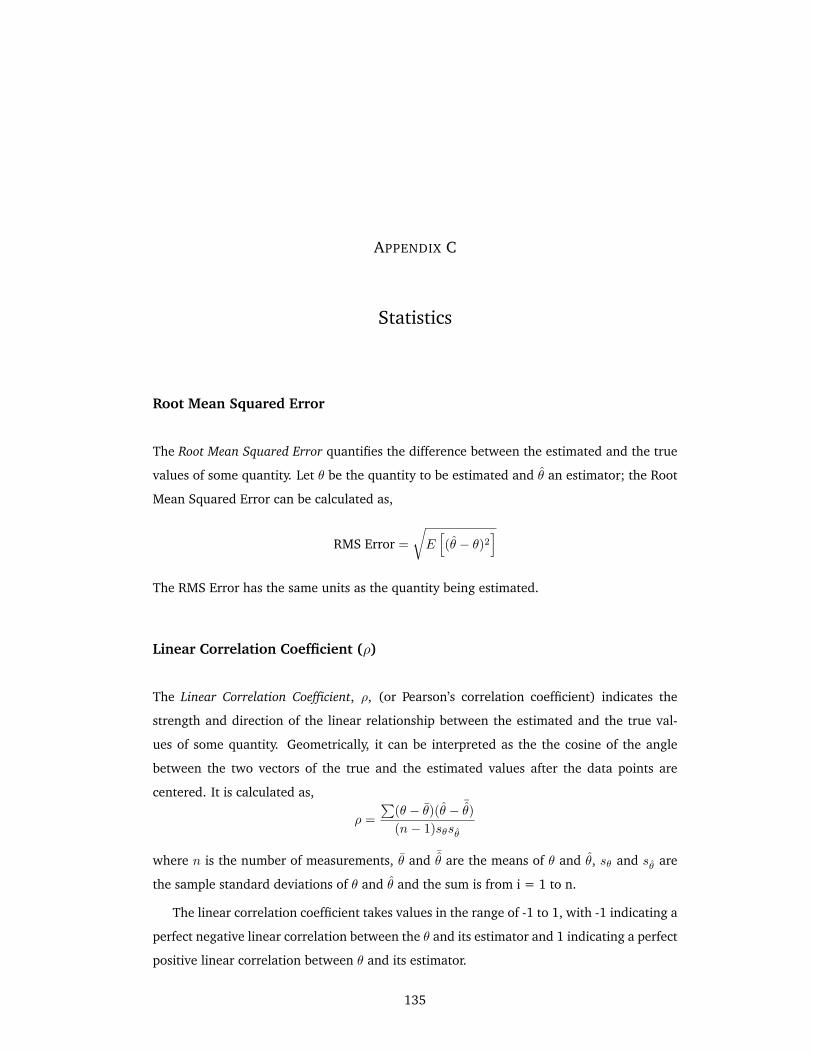
APPENDIX C
Statistics
Root Mean Squared Error
The Root Mean Squared Error quantifies the difference between the estimated and the true
values of some quantity. Let θ be the quantity to be estimated and θ an estimator; the Root
Mean Squared Error can be calculated as,
RMS Error =√
E[(θ − θ)2
]The RMS Error has the same units as the quantity being estimated.
Linear Correlation Coefficient (ρ)
The Linear Correlation Coefficient, ρ, (or Pearson’s correlation coefficient) indicates the
strength and direction of the linear relationship between the estimated and the true val-
ues of some quantity. Geometrically, it can be interpreted as the the cosine of the angle
between the two vectors of the true and the estimated values after the data points are
centered. It is calculated as,
ρ =∑
(θ − θ)(θ − ¯θ)
(n− 1)sθsθ
where n is the number of measurements, θ and ¯θ are the means of θ and θ, sθ and sθ are
the sample standard deviations of θ and θ and the sum is from i = 1 to n.
The linear correlation coefficient takes values in the range of -1 to 1, with -1 indicating a
perfect negative linear correlation between the θ and its estimator and 1 indicating a perfect
positive linear correlation between θ and its estimator.
135
136 APPENDIX C. STATISTICS
Kendall’s tau (τ)
The Kendall’s τ statistic is a non-parametric statistic used to quantify the correlation between
two rankings. It is a function of the minimum number of pairwise adjacent interchanges
needed to convert one ranking into the other. Given two ranked lists of length N, let C
be the total number of concordant pairs (pairs that are ranked in the same order in both
rankings) and D be the total number of discordant pairs (pairs that are ranked in opposite
order in the two rankings). Then, the Kendalls τ can be computed as,
τ =C −D
N(N − 1)/2
If the two rankings are exactly the same, then the Kendalls τ value is 1. If the two
rankings perfectly disagree with each other, then the Kendalls τ value is 1 and if the two
rankings are completely independent of each other (no correlation), then the Kendalls τ
value is 0.