Building Envelope Impact On HVAC Energy Use€¦ · · 2016-09-22Building Envelope Impact On HVAC...

Building Envelope Impact On HVAC Energy Use

Course# ME701

EZ-pdh.com Ezekiel Enterprises, LLC 301 Mission Dr. Unit 571

New Smyrna Beach, FL 32128 386-882-EZCE(3923) [email protected]

Ezekiel Enterprises, LLC

CAirtig

Investigation of the Impact ofommercial Building Envelopehtness on HVAC Energy Use

Steven J. EmmerichTim McDowell

Wagdy Anis

NISTIR 7238

8

Investigation of theCommercial Building

Airtightness on HVAC E

Building and

Shepley Bulfi

U

Office

Phillip J. Bond, Under Secre

National Institu

H

NISTIR 723

Impact of Envelopenergy Use

Steven J. Emmerich Fire Research Laboratory

Timothy P. McDowellTESS, Inc.

Wagdy Anisnch Richardson and Abbott

Prepared for:

.S. Department of Energy

of Building Technologies

June 2005

U.S. Department of Commerce

Carlos M. Gutierrez, Secretary

Technology Administration

tary of Commerce for Technology

te of Standards and Technology

ratch Semerjian, Acting Director

ABSTRACT This report presents a simulation study of the energy impact of improving envelope airtightness in U.S. commercial buildings. Despite common assumptions, measurements have shown that typical U.S. commercial buildings are not particularly airtight. Past simulation studies have shown that commercial building envelope leakage can result in significant heating and cooling loads. To evaluate the potential energy savings of an effective air barrier requirement, annual energy simulations were prepared for three nonresidential buildings (a two-story office building, a one-story retail building, and a four-story apartment building) in 5 U.S. cities. A coupled multizone airflow and building energy simulation tool was used to predict the energy use for the buildings at a target tightness level relative to a baseline level based on measurements in existing buildings. Based on assumed blended national average heating and cooling energy prices, predicted potential annual heating and cooling energy cost savings ranged from 3 % to 36 % with the smallest savings occurring in the cooling-dominated climates of Phoenix and Miami. In order to put these estimated energy savings in context, a cost effectiveness calculation was performed using the scalar ratio methodology employed by ASHRAE SSPC 90.1.

Keywords: energy efficiency, infiltration, office buildings, ventilation

iii

TABLE OF CONTENTS ABSTRACT iii

INTRODUCTION 1

ANALYSIS METHOD 2

BUILDING DESCRIPTIONS 3

AIRFLOW MODELS 16

SYSTEM MODELS 18

SCALAR CALCULATION 19

RESULTS 21

DISCUSSION 34

ACKNOWLEDGEMENTS 35

REFERENCES 36

Appendix A: Commercial Building Airtightness Data 39

iv

Introduction The objective of this study is to investigate the impact of envelope airtightness on the energy consumption of typical commercial buildings in the U.S. Despite common assumptions that envelope air leakage is not significant in office and other commercial buildings, measurements have shown that these buildings are subject to larger infiltration rates than commonly believed (Persily 1998, Proskiw and Phillips 2001). Infiltration in commercial buildings can have many negative consequences, including reduced thermal comfort, interference with the proper operation of mechanical ventilation systems, degraded indoor air quality, moisture damage of building envelope components, and increased energy consumption. For these reasons, attention has been given to methods of improving airtightness both in existing buildings and new constructions (Persily 1993). Since 1997, the Building Environment and Thermal Envelope Council of the National Institute of Building Sciences has sponsored several symposia in the U.S. on the topic of air barriers for buildings in North American climates. Canada Mortgage and Housing Corporation has sponsored similar conferences in Canada. Others have also published articles on the importance of air leakage in commercial buildings (Anis 2001, Ask 2003). However, the focus of these conferences and publications has largely been air barrier technology and the non-energy impacts of air leakage in buildings. In order to evaluate the cost effectiveness of such measures to tighten buildings, estimates of the impact of air leakage on energy use are needed. An earlier study estimated the national impact of infiltration in office buildings based on a simplified method for calculating both the infiltration flows and the building energy use (Emmerich et al. 1995). The loads were calculated for a set of 25 buildings, each representing a certain percentage of the total office building stock of the United States. Twenty of these buildings represent the existing office building stock as of 1979 (Briggs, Crawley, and Schliesing 1992) and five represent construction between 1980 and 1995 (Crawley and Schliesing 1992). Further work improved on this initial method by using airflows from multi-zone airflow simulations (Emmerich and Persily 1998) combined with a simple load calculation. More recently, a more detailed analysis method to determine the impact of infiltration and ventilation rates on building energy usage was developed (McDowell et al. 2003). This approach included the coupling of a detailed multi-zone airflow model based on the CONTAMW model (Dols and Walton 2002) and the detailed multi-zone building energy modeling program TRNSYS (Klein 2000). This project demonstrated the ability of the coupled programs to study the annual heating and cooling energy use in the US office building stock as a function of infiltration and ventilation rates. The American Society of Heating, Refrigerating, and Air-Conditioning Engineers (ASHRAE) Standard 90.1 Envelope Subcommittee has formed a task group to consider updating the building air leakage requirements in the standard to require a continuous air barrier system. An air barrier system is the combination of interconnected materials, flexible joint systems, and components of the building envelope that provide the air-tightness of the building. Included in the current standard are detailed quantitative limits for air leakage through fenestration and doors but only general qualitative guidance for the opaque portion of the building envelope (ASHRAE 2001b). For example, the Standard requires sealing, caulking, gasketing, or weather-stripping such locations as joints around fenestration and doors, junctions between floors, walls, and roofs, etc. However, there is no quantitative air leakage limit specified for either the wall and other envelope components or the building as a whole. This is analogous to requiring that care be taken when installing insulation without requiring any minimum R-value.

1

Analysis Method To provide input to the ASHRAE 90.1 Envelope Subcommittee in its consideration of the potential energy savings and cost effectiveness of an effective air barrier requirement, annual energy simulations and cost estimates were prepared for three common, modern nonresidential buildings – a two-story office building, a one-story retail building, and a four-story apartment building. The apartment building is included because the scope of Standard 90.1 includes multi-family structures of more than three stories above grade. The new combined airflow-building energy modeling tool (described by McDowell et al. 2003) was used to estimate the energy impact of envelope airtightness in multiple U.S. climate types. HVAC systems representative of the types used in these buildings were included in the building models. Other building model parameters were chosen such that the buildings would be considered typical new construction and meet current ASHRAE Standard 90.1 requirements. Energy simulations were performed using TRNSYS (Klein 2000) - a transient system simulation program with a modular structure that was designed to solve complex energy system problems by dividing the problem into a series of smaller components. Each of these components can then be solved independently and coupled with other components to simulate and solve the larger system problem. Components (or Types as they are called) in TRNSYS may be as simple as a pump or pipe, or as complicated as a multi-zone building model. The entire program is then a collection of energy system component models grouped around a simulation engine (solver). The modular nature of the program makes it easier to add content to the program by introducing new component models to the standard package. The simulation engine provides the capability of interconnecting system components in any desired manner, solving differential equations, and facilitating inputs and outputs. The TRNSYS multi-zone building model (called Type 56) includes heat transfer by conduction, convection and radiation, heat gains due to the presence of occupants and equipment, and the storage of heat in the room air and building mass. The infiltration in the buildings was modeled using a TRNSYS type based on an updated version of the AIRNET model (Walton 1989), which is included in the multizone airflow and contaminant dispersal program CONTAMW (Dols and Walton 2002). CONTAMW combines the best available algorithms for modeling airflow and contaminant transport in multizone buildings with a graphic interface for data input and display of results. The multizone approach is implemented by constructing a network of elements describing the flow paths (HVAC ducts, doors, windows, cracks, etc.) between the zones of a building. The network nodes represent the zones, each of which are modeled at a uniform temperature and pollutant concentration. The pressures vary hydrostatically, so the zone pressure values are a function of the elevation within the zone. The network of equations is then solved at each time step of the simulation. McDowell et al. (2003) described the coupling of the TRNSYS and CONTAM models. Simulations of annual energy use were run using TMY2 files (Marion and Urban 1995) for five different cities representing different climate zones of the US (Miami, Phoenix, St. Louis, Bismarck, and Minneapolis) and at three levels of airtightness representing different construction practices. The levels of airtightness were selected to represent 1) no air barrier, 2) target air barrier, and 3) best achievable levels through a review of measured commercial building airtightness data (Persily 1998), ASHRAE Handbook data (ASHRAE 2001c) and other sources. Each building was modeled once with frame construction and then masonry construction. Thus, the matrix of simulations is 3 building types X 2 envelope construction types X 3 airtightness levels X 5 climates, for a total of 90 simulation cases.

2

Building Descriptions This section describes the three buildings modeled in the study. Thermal Properties, Setpoints, and Schedules The building models were developed so that the wall constructions and windows would satisfy the requirements of ASHRAE Standard 90.1 (ASHRAE 90.1-2001b) for the different locations as described below. Office Building The building modeled is a two story office building with a total floor area of 2250 m2 (24,200 ft2) and a floorplan as shown in Figure 1. The building has a window-to-wall ratio of 0.2 with a floor-to-floor height of 3.66 m (12 ft), broken up between a 2.74 m (9 ft) occupied floor and a 0.92 m (3 ft) plenum per floor.

The building also includes a single elevator shaft.

igure 1 Floorplan of two-story office building

odeling the office building are summarized

l, roof, slab and window thermal properties for office building

ix Thickness Conductivity Density Specific Heat Resistance

Floor Plenum4.6 m

33.5 m

24.4 m

B

L R

F

I

E

4.6 m 4.6 m

4.6 m

3.0 m

P

E

0.9 m

2.7 m

Plenum

Plenum

Floor 1

Floor 2

2.7 m

0.9 m

F, R, B, L are the front, right, back, and left perimeter zones.I is the core zone. E is the elevator zone.

F

The wall, roof, slab and window thermal properties used for min Table 1.

Table 1 Wal

Frame Wall Construction: St. Louis, Miami and PhoenDescription

m (ft)

W/m-K (Btu/hr-ft-F) (Btu/lb-F) (h )

kg/m3 (lb/ft3)

kJ/kg-K m2-K/W r-ft2-F/Btu

Face brick 0.092 (0.508) (0.59) (0.302) 0.879 1922

(120) 0.921 (0.22)

0.10

Vertical wall air layer (0.89)

0.16

Gypsum board 0.0127 (0.0417)

0.160 (0.0926)

800 0.837 (50) (0.2)

0.079 (0.45)

Steel studs w/mineral wool insulation, R13

0.089 (0.292)

0.0751 (0.0434)

288 (18)

1.298 (0.31)

1.2 (6.7)

Gypsum board (0.0521) (0.0926) 0.0159 0.160 800

(50) 0.837 (0.2)

0.099 (0.56)

3

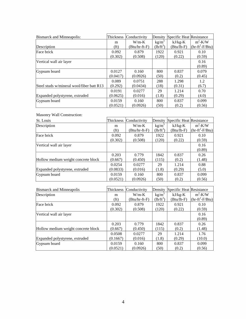
Bismarck and Minneapolis: Thickness Conductivity Density Specific Heat Resistance

Description m

(ft) W/m-K

(Btu/hr-ft-F) kg/m3

(lb/ft3)kJ/kg-K

(Btu/lb-F) m2-K/W

(hr-ft2-F/Btu)Face brick

0.092 (0.302)

0.879 (0.508)

1922 (120)

0.921 (0.22)

0.10 (0.59)

Vertical wall air layer

0.16 (0.89)

Gypsum board

0.0127 (0.0417)

0.160 (0.0926)

800 (50)

0.837 (0.2)

0.079 (0.45)

Steel studs w/mineral wool/fiber batt R13 0.089

(0.292) 0.0751

(0.0434) 288 (18)

1.298 (0.31)

1.2 (6.7)

Expanded polystyrene, extruded 0.0191

(0.0625) 0.0277 (0.016)

29 (1.8)

1.214 (0.29)

0.70 (4.0)

Gypsum board

0.0159 (0.0521)

0.160 (0.0926)

800 (50)

0.837 (0.2)

0.099 (0.56)

Masonry Wall Construction: St. Louis Thickness Conductivity Density Specific Heat Resistance Description

m (ft)

W/m-K (Btu/hr-ft-F)

kg/m3 (lb/ft3)

kJ/kg-K (Btu/lb-F)

m2-K/W (hr-ft2-F/Btu)

Face brick

0.092 (0.302)

0.879 (0.508)

1922 (120)

0.921 (0.22)

0.10 (0.59)


0.16 (0.89)

Hollow medium weight concrete block 0.203

(0.667) 0.779

(0.450) 1842 (115)

0.837 (0.2)

0.26 (1.48)


(0.0833) 0.0277 (0.016)

29 (1.8)

1.214 (0.29)

0.88 (5.0)

Gypsum board

0.0159 (0.0521)

0.160 (0.0926)

800 (50)

0.837 (0.2)

0.099 (0.56)

Bismarck and Minneapolis Thickness Conductivity Density Specific Heat Resistance Description

m (ft)

W/m-K (Btu/hr-ft-F)

kg/m3 (lb/ft3)

kJ/kg-K (Btu/lb-F)


Face brick

0.092 (0.302)

0.879 (0.508)

1922 (120)

0.921 (0.22)

0.10 (0.59)


0.16 (0.89)


(0.667) 0.779

(0.450) 1842 (115)

0.837 (0.2)

0.26 (1.48)


(0.1667) 0.0277 (0.016)

29 (1.8)

1.214 (0.29)

1.76 (10.0)

Gypsum board

0.0159 (0.0521)

0.160 (0.0926)

800 (50)

0.837 (0.2)

0.099 (0.56)

4

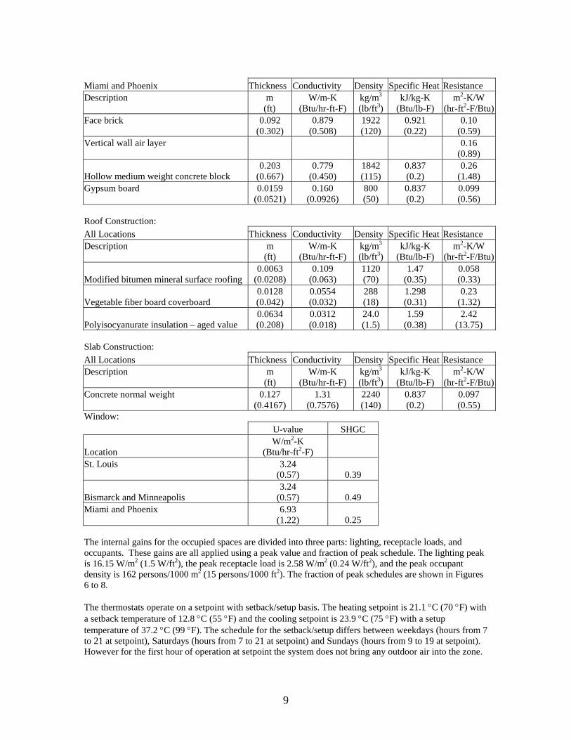
Miami and Phoenix Thickness Conductivity Density Specific Heat Resistance Description

m (ft)

W/m-K (Btu/hr-ft-F)

kg/m3 (lb/ft3)

kJ/kg-K (Btu/lb-F)


Face brick

0.092 (0.302)

0.879 (0.508)

1922 (120)

0.921 (0.22)

0.10 (0.59)


0.16 (0.89)


(0.667) 0.779

(0.450) 1842 (115)

0.837 (0.2)

0.26 (1.48)

Gypsum board

0.0159 (0.0521)

0.160 (0.0926)

800 (50)

0.837 (0.2)

0.099 (0.56)

Roof Construction: All Locations Thickness Conductivity Density Specific Heat Resistance

Description m

(ft) W/m-K

(Btu/hr-ft-F) kg/m3

(lb/ft3)kJ/kg-K

(Btu/lb-F) m2-K/W

(hr-ft2-F/Btu)Built-up roofing

0.0095 (0.0313)

1.63 (0.939)

1120 (70)

1.47 (0.35)

0.058 (0.33)

Polyisocyanurate insulation

0.0634 (0.208)

0.0242 (0.014)

24 (1.5)

1.59 (0.38)

2.62 (14.85)

Vegetable Fiber Board Sheathing 0.0128 (0.042)

0.0554 (0.032)

288 (18)

1.298 (0.31)

0.23 (1.32)

Slab Construction: All Locations Thickness Conductivity Density Specific Heat Resistance

Description m

(ft) W/m-K

(Btu/hr-ft-F) kg/m3

(lb/ft3)kJ/kg-K

(Btu/lb-F) m2-K/W

(hr-ft2-F/Btu)

Concrete normal weight 0.127

(0.4167) 1.31

(0.7576) 2240 (140)

0.837 (0.2)

0.097 (0.55)

Window: U-value SHGC

Location W/m2-K

(Btu/hr-ft2-F) St. Louis, Bismarck, and Minneapolis

3.24 (0.57) 0.39

Miami and Phoenix

6.93 (1.22) 0.25

The internal gains for the occupied spaces are divided into three parts: lighting, receptacle loads, and occupants. These gains are all applied using a peak value and fraction of peak schedule. The lighting peak is 10.8 W/m2 (1.0 W/ft2), the peak receptacle load is 6.8 W/m2 (0.63 W/ft2), and the peak occupant density is 53.4 persons/1000 m2 (5 persons/1000 ft2). The fraction of peak schedules are shown in Figures 2 to 4. The thermostats operate on a setpoint with setback/setup basis. The heating setpoint is 21.1 °C (70 °F) with a setback temperature of 12.8 °C (55 °F) and the cooling setpoint is 23.9 °C (75 °F) with a setup temperature of 32.2 °C (90 °F). The schedule for the setback/setup differs between weekdays (hours from 6 to 20 at setpoint), Saturdays (hours from 7 to 14 at setpoint) and Sundays (always at setup/setback). However, for the first hour of operation at setpoint, the system does not bring any outdoor air into the zone. This hour is prior to building occupancy and is used to bring the zone back to setpoint from the setup/setback temperature.

5

0

0.1

0.2

0.3

0.4

0.5

0.6

0.7

0.8

0.9

1

1 2 3 4 5 6 7 8 9 10 11 12 13 14 15 16 17 18 19 20 21 22 23 24

Hour of Day

Frac

tion

of P

eak

Occ

upan

cy

Weekday

Saturday

Sunday

Figure 2 Fractional occupancy schedule for office

0

0.1

0.2

0.3

0.4

0.5

0.6

0.7

0.8

0.9

1

1 2 3 4 5 6 7 8 9 10 11 12 13 14 15 16 17 18 19 20 21 22 23 24

Hour of Day

Frac

tion

of P

eak

Ligh

ting

Weekday

Saturday

Sunday

Figure 3 Fractional lighting schedule for office

0

0.1

0.2

0.3

0.4

0.5

0.6

0.7

0.8

0.9

1

1 2 3 4 5 6 7 8 9 10 11 12 13 14 15 16 17 18 19 20 21 22 23 24

Hour of Day

Frac

tion

of P

eak

Rec

epta

cle

Load

Weekday

Saturday

Sunday

Figure 4 Fractional receptacle load schedule for office

6

Retail Building The retail building modeled in this study is a one-story building with a total floor area of 1125 m2 (12,100 ft2) and a floorplan as shown in Figure 5. The building has a window-to-wall ratio of 0.1 with a floor-to-floor height of 3.9 m (13 ft), broken up between a 3.0 m (10 ft) occupied floor and a 0.9 m (3 ft) plenum

per floor.

igure 5 Floorplan of one-story retail building

he wall, roof, slab and window thermal properties used in modeling the retail building are summarized in

all, roof, slab and window thermal properties for retail building

ix Thickness Conductivity Density Specific Heat Resistance

Floor Plenum4.6 m

33.5 m

24.4 m

B

L R

F

I

4.6 m 4.6 m

4.6 m

P

Plenum

Floor 1 3.0 m

0.9 m

F, R, B, L are the front, right, back, and left perimeter zones.I is the core zone.

F

TTable 2.

Table 2 W

Frame Wall Construction: St. Louis, Miami and PhoenDescription

m (ft)

W/m-K (Btu/hr-ft-F) (Btu/lb-F) (h )

kg/m3 (lb/ft3)

kJ/kg-K m2-K/W r-ft2-F/Btu

Face brick 0.092 (0.508) (0.59) (0.302) 0.879 1922

(120) 0.921 (0.22)

0.10

Vertical wall air layer (0.89)

0.16

Gypsum board 0.0127 (0.0417)

0.160 (0.0926)

800 0.837 (50) (0.2)

0.079 (0.45)

Steel studs w/mineral wool/fiber batt R-13 (8.06) 0.089

(0.292) 0.0627

(0.0362) 9.6

(0.6) 0.837 (0.2)

1.42

Gypsum board

0.0159 (0.0521) (0.0926)

0.160 800 (50)

0.837 (0.2)

0.099 (0.56)

7

Bismarck and Minneapolis Thickness Conductivity Density Specific Heat Resistance

Description m

(ft) W/m-K

(Btu/hr-ft-F) kg/m3

(lb/ft3)kJ/kg-K

(Btu/lb-F) m2-K/W

(hr-ft2-F/Btu)Face brick

0.092 (0.302)

0.879 (0.508)

1922 (120)

0.921 (0.22)

0.10 (0.59)


0.16 (0.89)

Gypsum board

0.0127 (0.0417)

0.160 (0.0926)

800 (50)

0.837 (0.2)

0.079 (0.45)

Steel studs w/mineral wool/fiber batt R-130.089

(0.292) 0.0627

(0.0362) 9.6

(0.6) 0.837 (0.2)

1.42 (8.06)


(0.0625) 0.0277 (0.016)

29 (1.8)

1.214 (0.29)

0.70 (4.0)

Gypsum board

0.0159 (0.0521)

0.160 (0.0926)

800 (50)

0.837 (0.2)

0.099 (0.56)

Masonry Wall Construction: St. Louis Thickness Conductivity Density Specific Heat Resistance Description

m (ft)

W/m-K (Btu/hr-ft-F)

kg/m3 (lb/ft3)

kJ/kg-K (Btu/lb-F)


Face brick

0.092 (0.302)

0.879 (0.508)

1922 (120)

0.921 (0.22)

0.10 (0.59)


0.16 (0.89)


(0.667) 0.779

(0.450) 1842 (115)

0.837 (0.2)

0.26 (1.48)


(0.0833) 0.0277 (0.016)

29 (1.8)

1.214 (0.29)

0.88 (5.0)

Gypsum board

0.0159 (0.0521)

0.160 (0.0926)

800 (50)

0.837 (0.2)

0.099 (0.56)

Bismarck and Minneapolis Thickness Conductivity Density Specific Heat Resistance Description

m (ft)

W/m-K (Btu/hr-ft-F)

kg/m3 (lb/ft3)

kJ/kg-K (Btu/lb-F)


Face brick

0.092 (0.302)

0.879 (0.508)

1922 (120)

0.921 (0.22)

0.10 (0.59)


0.16 (0.89)


(0.667) 0.779

(0.450) 1842 (115)

0.837 (0.2)

0.26 (1.48)


(0.1667) 0.0277 (0.016)

29 (1.8)

1.214 (0.29)

1.76 (10.0)

Gypsum board

0.0159 (0.0521)

0.160 (0.0926)

800 (50)

0.837 (0.2)

0.099 (0.56)

8

Miami and Phoenix Thickness Conductivity Density Specific Heat Resistance Description

m (ft)

W/m-K (Btu/hr-ft-F)

kg/m3 (lb/ft3)

kJ/kg-K (Btu/lb-F)


Face brick

0.092 (0.302)

0.879 (0.508)

1922 (120)

0.921 (0.22)

0.10 (0.59)


0.16 (0.89)


(0.667) 0.779

(0.450) 1842 (115)

0.837 (0.2)

0.26 (1.48)

Gypsum board

0.0159 (0.0521)

0.160 (0.0926)

800 (50)

0.837 (0.2)

0.099 (0.56)

Roof Construction: All Locations Thickness Conductivity Density Specific Heat Resistance Description

m (ft)

W/m-K (Btu/hr-ft-F)

kg/m3

(lb/ft3)kJ/kg-K

(Btu/lb-F) m2-K/W

(hr-ft2-F/Btu)

Modified bitumen mineral surface roofing 0.0063

(0.0208) 0.109

(0.063) 1120 (70)

1.47 (0.35)

0.058 (0.33)

Vegetable fiber board coverboard 0.0128 (0.042)

0.0554 (0.032)

288 (18)

1.298 (0.31)

0.23 (1.32)

Polyisocyanurate insulation – aged value 0.0634 (0.208)

0.0312 (0.018)

24.0 (1.5)

1.59 (0.38)

2.42 (13.75)

Slab Construction: All Locations Thickness Conductivity Density Specific Heat Resistance Description

m (ft)

W/m-K (Btu/hr-ft-F)

kg/m3

(lb/ft3)kJ/kg-K

(Btu/lb-F) m2-K/W

(hr-ft2-F/Btu)Concrete normal weight

0.127 (0.4167)

1.31 (0.7576)

2240 (140)

0.837 (0.2)

0.097 (0.55)


Location W/m2-K

(Btu/hr-ft2-F) St. Louis

3.24 (0.57) 0.39

Bismarck and Minneapolis 3.24

(0.57) 0.49 Miami and Phoenix

6.93 (1.22) 0.25

The internal gains for the occupied spaces are divided into three parts: lighting, receptacle loads, and occupants. These gains are all applied using a peak value and fraction of peak schedule. The lighting peak is 16.15 W/m2 (1.5 W/ft2), the peak receptacle load is 2.58 W/m2 (0.24 W/ft2), and the peak occupant density is 162 persons/1000 m2 (15 persons/1000 ft2). The fraction of peak schedules are shown in Figures 6 to 8. The thermostats operate on a setpoint with setback/setup basis. The heating setpoint is 21.1 °C (70 °F) with a setback temperature of 12.8 °C (55 °F) and the cooling setpoint is 23.9 °C (75 °F) with a setup temperature of 37.2 °C (99 °F). The schedule for the setback/setup differs between weekdays (hours from 7 to 21 at setpoint), Saturdays (hours from 7 to 21 at setpoint) and Sundays (hours from 9 to 19 at setpoint). However for the first hour of operation at setpoint the system does not bring any outdoor air into the zone.

9

This hour is prior to building occupancy and is used to bring the zone back to setpoint from the setup/setback temperature.

0

0.1

0.2

0.3

0.4

0.5

0.6

0.7

0.8

0.9

1

1 2 3 4 5 6 7 8 9 10 11 12 13 14 15 16 17 18 19 20 21 22 23 24

Hour of Day

Frac

tion

of P

eak

Occ

upan

cy

Weekday

Saturday

Sunday

Figure 6 Fractional occupancy schedule for retail

0

0.1

0.2

0.3

0.4

0.5

0.6

0.7

0.8

0.9

1

1 2 3 4 5 6 7 8 9 10 11 12 13 14 15 16 17 18 19 20 21 22 23 24

Hour of Day

Frac

tion

of P

eak

Ligh

ting

Weekday

Saturday

Sunday

Figure 7 Fractional lighting schedule for retail

0

0.1

0.2

0.3

0.4

0.5

0.6

0.7

0.8

0.9

1

1 2 3 4 5 6 7 8 9 10 11 12 13 14 15 16 17 18 19 20 21 22 23 24

Hour of Day

Frac

tion

of P

eak

Rec

epta

cle

Load

Weekday

Saturday

Sunday

Figure 8 Fractional receptacle load schedule for retail

10

Residential Building The residential building modeled in this study is a four story building with a total floor area of 3425 m2 (36,864 ft2) and a floorplan as shown in Figure 9. The building has a window-to-wall ratio of 0.25 with a floor-to-floor height of 3.0 m (10 ft), broken up between a 2.4 m (8 ft) occupied floor and a 0.6 m (2 ft) plenum for the bottom three floors and a 2.4 m (8 ft) occupied floor and a 3.0m (10 ft) attic at the top. The attic has a pitched roof and is vented. The building also includes a single elevator shaft with two elevators. The corner units will have a doorway connecting to the corridor. One of bottom mid-units is used as a lobby entrance instead of a living unit.

9.8 m

6.1m

E3.0m

Unit BL Unit BM Unit BR

Unit LM

Corridor

Unit RM

Unit FL Unit FM Unit FR

9.8 m 9.8 m

9.8 m

9.8 m

9.8 m

9.8 m

6.1m

E3.0m

Plenum BL Plenum BM Plenum BR

Plenum LM

Core Plenum

Plenum RM

Plenum FL Plenum FM Plenum FR

9.8 m 9.8 m

9.8 m

9.8 m

9.8 m

Ceiling Space

Floor 3Ceiling Space

Floor 2Ceiling Space

Floor 1

Floor 4

Attic

2.4 m

0.6 m

2.4 m

0.6 m

2.4 m

0.6 m

2.4 m

3.0 m

Figure 9 Floorplan of modeled four-story residential building

The wall, roof, slab and window thermal properties used for modeling the apartment building are summarized in Table 3.

11

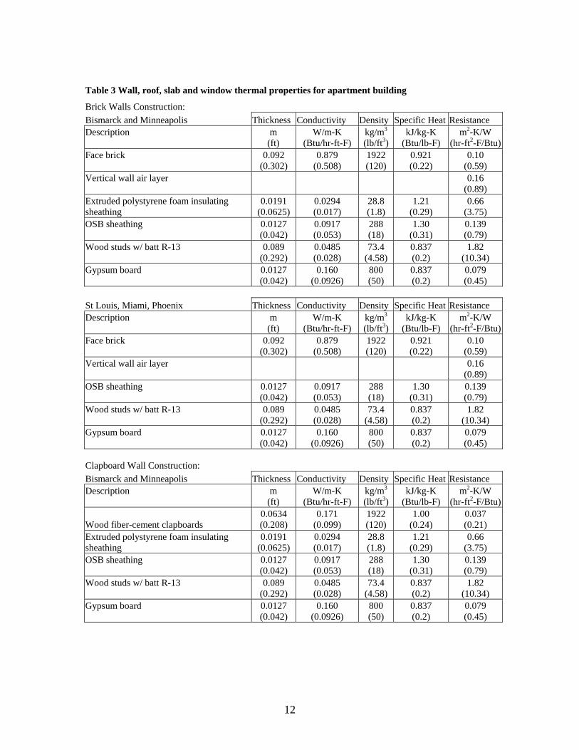
Table 3 Wall, roof, slab and window thermal properties for apartment building

Brick Walls Construction: Bismarck and Minneapolis Thickness Conductivity Density Specific Heat Resistance Description

m (ft)

W/m-K (Btu/hr-ft-F)

kg/m3 (lb/ft3)

kJ/kg-K (Btu/lb-F)


Face brick

0.092 (0.302)

0.879 (0.508)

1922 (120)

0.921 (0.22)

0.10 (0.59)


0.16 (0.89)

Extruded polystyrene foam insulating sheathing

0.0191 (0.0625)

0.0294 (0.017)

28.8 (1.8)

1.21 (0.29)

0.66 (3.75)

OSB sheathing

0.0127 (0.042)

0.0917 (0.053)

288 (18)

1.30 (0.31)

0.139 (0.79)

Wood studs w/ batt R-13

0.089 (0.292)

0.0485 (0.028)

73.4 (4.58)

0.837 (0.2)

1.82 (10.34)

Gypsum board

0.0127 (0.042)

0.160 (0.0926)

800 (50)

0.837 (0.2)

0.079 (0.45)

St Louis, Miami, Phoenix Thickness Conductivity Density Specific Heat Resistance Description

m (ft)

W/m-K (Btu/hr-ft-F)

kg/m3 (lb/ft3)

kJ/kg-K (Btu/lb-F)


Face brick

0.092 (0.302)

0.879 (0.508)

1922 (120)

0.921 (0.22)

0.10 (0.59)


0.16 (0.89)

OSB sheathing

0.0127 (0.042)

0.0917 (0.053)

288 (18)

1.30 (0.31)

0.139 (0.79)


0.089 (0.292)

0.0485 (0.028)

73.4 (4.58)

0.837 (0.2)

1.82 (10.34)

Gypsum board

0.0127 (0.042)

0.160 (0.0926)

800 (50)

0.837 (0.2)

0.079 (0.45)

Clapboard Wall Construction: Bismarck and Minneapolis Thickness Conductivity Density Specific Heat Resistance Description

m (ft)

W/m-K (Btu/hr-ft-F)

kg/m3 (lb/ft3)

kJ/kg-K (Btu/lb-F)


Wood fiber-cement clapboards 0.0634 (0.208)

0.171 (0.099)

1922 (120)

1.00 (0.24)

0.037 (0.21)

Extruded polystyrene foam insulating sheathing

0.0191 (0.0625)

0.0294 (0.017)

28.8 (1.8)

1.21 (0.29)

0.66 (3.75)

OSB sheathing

0.0127 (0.042)

0.0917 (0.053)

288 (18)

1.30 (0.31)

0.139 (0.79)


0.089 (0.292)

0.0485 (0.028)

73.4 (4.58)

0.837 (0.2)

1.82 (10.34)

Gypsum board

0.0127 (0.042)

0.160 (0.0926)

800 (50)

0.837 (0.2)

0.079 (0.45)

12

St Louis, Miami, Phoenix Thickness Conductivity Density Specific Heat Resistance Description

m (ft)

W/m-K (Btu/hr-ft-F)

kg/m3 (lb/ft3)

kJ/kg-K (Btu/lb-F)


Wood fiber-cement clapboards 0.0634 (0.208)

0.171 (0.099)

1922 (120)

1.00 (0.24)

0.037 (0.21)

OSB sheathing

0.0127 (0.042)

0.0917 (0.053)

288 (18)

1.30 (0.31)

0.139 (0.79)


0.089 (0.292)

0.0485 (0.028)

73.4 (4.58)

0.837 (0.2)

1.82 (10.34)

Gypsum board

0.0127 (0.042)

0.160 (0.0926)

800 (50)

0.837 (0.2)

0.079 (0.45)

Roof Construction: All Locations Thickness Conductivity Density Specific Heat Resistance Description

m (ft)

W/m-K (Btu/hr-ft-F)

kg/m3

(lb/ft3)kJ/kg-K

(Btu/lb-F) m2-K/W

(hr-ft2-F/Btu)Asphalt shingles

0.0114 (0.0375)

1.475 (0.852)

1120 (70)

1.47 (0.35)

0.078 (0.44)

Oriented strand board (waferboard) sheathing

0.0128 (0.042)

0.0917 (0.053)

288 (18)

1.298 (0.31)

0.14 (0.79)

Top Floor Ceiling Construction: All Locations Thickness Conductivity Density Specific Heat Resistance Description

m (ft)

W/m-K (Btu/hr-ft-F)

kg/m3

(lb/ft3)kJ/kg-K

(Btu/lb-F) m2-K/W

(hr-ft2-F/Btu)Insulated wood trusses

0.254 (0.833)

0.0389 (0.0225)

57.5 (3.59)

0.837 (0.2)

6.52 (37.04)

Slab Construction: All Locations Thickness Conductivity Density Specific Heat Resistance Description

m (ft)

W/m-K (Btu/hr-ft-F)

kg/m3

(lb/ft3)kJ/kg-K

(Btu/lb-F) m2-K/W

(hr-ft2-F/Btu)Concrete normal weight

0.127 (0.4167)

1.31 (0.7576)

2240 (140)

0.837 (0.2)

0.097 (0.55)

Floor Construction: All Locations Thickness Conductivity Density Specific Heat Resistance Description

m (ft)

W/m-K (Btu/hr-ft-F)

kg/m3 (lb/ft3)

kJ/kg-K (Btu/lb-F)


Gypcrete

0.0128 (0.042)

0.160 (0.0926)

800 (50)

0.84 (0.2)

0.079 (0.45)

Plywood

0.0191 (0.0625)

0.116 (0.0669)

545 (34)

1.21 (0.29)

0.164 (0.93)

Wood Joists w/acoustic batts

0.254 (0.833)

0.0673 (0.0389)

57.5 (3.59)

1.67 (0.4)

3.78 (21.44)

13

Ceiling (except top floor) Construction: All Locations Thickness Conductivity Density Specific Heat Resistance Description

m (ft)

W/m-K (Btu/hr-ft-F)

kg/m3

(lb/ft3)kJ/kg-K

(Btu/lb-F) m2-K/W

(hr-ft2-F/Btu)Gypsum board

0.0127 (0.042)

0.160 (0.0926)

800 (50)

0.837 (0.2)

0.079 (0.45)


Location W/m2-K

(Btu/hr-ft2-F)

St. Louis, Bismarck, and Minneapolis 3.80

(0.67) 0.39 Miami and Phoenix

7.21 (1.27) 0.25

The internal gains for the occupied spaces are calculated based on a total sensible heat gain per day per unit to account for a combination of lights, people and equipment per the Space Conditioning calculation procedure of Standard 90.2 (ASHRAE 2001d). These gains equal 21,100 kJ (20,000 Btu) plus the floor area times 170 kJ/m2 (15 Btu/ft2) and are scheduled as shown in Figure 10. The total latent heat gains are assumed to be 0.2 times the sensible gains.

0

0.01

0.02

0.03

0.04

0.05

0.06

0.07

0 2 4 6 8 10 12 14 16 18 20 22 24Hour of day

Mul

tiplie

r for

inte

rnal

gai

ns

Figure 10 Residential building internal gains schedule

The thermostats operate on a setpoint with setback/setup basis. The heating setpoint is 20.0 °C (68 °F) and the cooling setpoint is 25.6 °C (78 °F). The schedule for the setback/setup for the living units is shown in Figure 11. The lobby and corridor zones are heated to 20.0 °C (68 °F) and cooled to 25.6 °C (78 °F).

14

0

5

10

15

20

25

30

0 2 4 6 8 10 12 14 16 18 20 22 24Hour of day

Tem

pera

ture

(°C

)

Workday_HeatWorkday_CoolWeekend_HeatWeekend_Cool

Figure 11 Thermostat schedule for residential building

15

Airflow Models This section provides the details of the airtightness levels used in the study. Three different airtightness levels (No air barrier, target, and best achievable) were modeled in each building by changing the leakage characteristics in the CONTAM multizone airflow models for each building. The values for the no air barrier level varied for each location, while the target and best achievable construction cases were the same for all locations. The values for the no air barrier (i.e., baseline) case were established through an analysis of the available published airtightness data for buildings other than low-rise residential buildings. The majority of the data were compiled in a 1998 summary (Persily 1998) supplemented by additional data including more Florida commercial buildings, additional U.K. office buildings, and Canadian apartment buildings added during this study [see references in Appendix A]. The entire dataset of 166 buildings (144 in North America and 22 in U.K.) and the references are presented in Appendix A. This dataset includes all data from the ASHRAE Handbook of Fundamentals (ASHRAE 2001c) but adds data from over 150 additional buildings reported in 13 different studies. Since these data are intended to represent only the baseline case, no buildings known to have been constructed to a specific airtightness level are included. Most of the air leakage rates in the dataset were determined using ASTM E779 fan pressurization tests (ASTM 1999). Others were tested by very similar methods such as Canadian (CGSB 1986 and CGSB 1999), International (ISO 1996) or British (CIBSE 2000) standards. Proskiw and Philips (2001) summarize and compare these and other current or proposed building airtightness testing methods. As reference points, average airtightness levels from various subsets of the data, in units of L/s-m2 (cfm/ft2) at an indoor-outdoor pressure difference of 75 Pa (0.3 in H2O), normalized by above-grade envelope surface area are as follows:

NIST studies (U.S. office buildings): 4.2 L/s-m2 (0.83 cfm/ft2) Brennan paper (NY schools): 2.4 L/s-m2 (0.47 cfm/ft2) NRCC (Canadian large offices): 2.9 L/s-m2 (0.57 cfm/ft2) NRCC (Canadian schools): 7.9 L/s-m2 (1.6 cfm/ft2) NRCC (Canadian retail buildings): 13.7 L/s-m2 (2.7 cfm/ft2) Mulitple studies (Canadian apartment buildings): 3.1 L/s-m2 (0.61 cfm/ft2) BRE and BSRIA (U.K. office buildings): 7.2 L/s-m2 (1.4 cfm/ft2) FSEC studies (mixed small commercial): 12.6 L/s-m2 (2.5 cfm/ft2)

Based on the available information, the dataset was reduced by excluding buildings older than 1960 (even though examination of the data by U.S., Canadian and U.K. authors have found no trends toward increased airtightness in more recent buildings [Persily 1998, Proskiw and Phillips 2001, and Potter et al. 1995]), all industrial buildings, and one extremely leaky building. The data were then divided into north (Standard 90.1 climate zones 5 and above) and south (Standard 90.1 climate zones 4 and below) subsets for North American buildings only. Unfortunately, the available data are inadequate to support a breakdown by the individual climate zones. Finally, within those North and South subsets, average airtightness was calculated for short buildings (3 stories and less) and tall buildings (4 stories and up) as the data demonstrate that the tall buildings are tighter on average. The average airtightness values (again in units of L/s-m2 at 75 Pa (cfm/ft2 at 0.3 in H2O), normalized by above-grade envelope surface area) are as follows:

North_short (29 buildings): 6.6 L/s-m2 (1.3 cfm/ft2) South_short (74 buildings): 11.8 L/s-m2 (2.3 cfm/ft2)

Based on consideration of the available data, the average measured value from the short buildings in the south was used as the baseline value in the warmest climate (Miami) and the average measured value from the short buildings in the north was used as the baseline value in the coldest climate (Bismarck). The values for the remaining locations were assigned by linearly interpolating between these values using the number of heating degree days (HDD) for the location. As a result, the whole building air leakage values used were (in units of L/s-m2 at 75 Pa (cfm/ft2 @ 0.3 inH2O) and normalized by above-grade envelope surface area) as follows:

16

No air barrier: Miami 11.8 L/s-m2 (2.3 cfm/ft2) Phoenix 11.1 L/s-m2 (2.2 cfm/ft2) St. Louis 9.1 L/s-m2 (1.8 cfm/ft2) Minneapolis 7.2 L/s-m2 (1.4 cfm/ft2) Bismarck 6.6 L/s-m2 (1.3 cfm/ft2)

In addition to the baseline level, all buildings were modeled at two levels of increased airtightness. Both published building airtightness data and current commercial buildings airtightness standards were considered in selecting these levels. The ‘target’ level was selected to represent a level of airtightness that can be achieved through good construction practice, while the ‘best achievable’ level is based on the tightest levels reported for nonresidential buildings. Achieving the tightest level would require an aggressive program of quality control during construction and airtightness testing, combined with efforts to identify and repair any leaks.

Target: 1.2 L/s-m2 (0.24 cfm/ft2) Best achievable: 0.2 L/s-m2 (0.04 cfm/ft2)

About 6 % of the tested buildings listed in Appendix A would meet the 1.2 L/s-m2 (0.24 cfm/ft2) selected target airtightness level. Note that none of these tested buildings was built to an airtightness standard. For comparison, the average reported airtightness level was calculated for non-residential buildings in the U.K., Ireland, and Germany that were constructed to specified whole building airtightness targets as reported in Building Services Journal articles and elsewhere (Anon. 1998, Anon. 2002, Anon. 2003, Cohen 2003, Olivier 2001and Kennett 2004). These 14 buildings, which were of various envelope construction types (curtain wall, masonry, frame, and mixed) and ranged from 1 story to 6 stories, averaged 1.3 L/s-m2 at 75 Pa (0.25 cfm/ft2 at 0.3 inH2O). In addition to simulations at these levels, the ‘no air barrier’ and target levels were varied as part of a sensitivity analyses, as described below. Although the whole building air leakage dataset in Appendix A lacks data for U.S. apartment buildings, a literature review by Edwards (1999) reported air leakage for apartment units in 16 U.S. buildings from four studies (Modera et al. 1985, Diamond et al. 1986, Synertech 1987, Feustel and Diamond 1996). The average leakage of these 16 buildings was 20 cm2 per m2 (0.29 in2 per ft2) of floor area at 4 Pa. For the apartment building modeled in this study (and assuming uniform distribution over all apartment surfaces), this value corresponds to 11.6 L/s-m2 at 75 Pa (2.3 cfm/ft2 at 0.3 in H2O), which is leakier than the average value used in the models discussed above. Also, no direct leakage between adjacent units was assumed for the apartment building. Suite access doors from the hallways were modeled as an effective leakage area of 200 cm2 (31 in2) at 4 Pa based on measurements by Wray et al. (1998).

17

System Models The HVAC systems modeled were specified to be representative of systems that would be installed in typical practice. The systems were different for the different building types and were sized for the appropriate locations. Whether each system included an economizer for the different locations was based on the criteria in ASHRAE 90.1. Office Building: The office building system included water-source heat pumps (WSHPs) with a cooling tower and a boiler serving the common loop. Each zone had its own WSHP rejecting/extracting heat from the common loop. The outdoor air for each zone was supplied to each individual heat pump, and the heat pump blower was on at all times when the zone was occupied. When the location of the building required an economizer, the outdoor air controls were applied to the individual heat pump’s airflow. With this approach, different heat pumps could have a different percentage of outdoor air at the same time depending on the loads. For the five modeled locations, St. Louis, Bismarck and Phoenix included economizers and Minneapolis and Miami did not. Return airflow was specified to equal 95 % of supply airflow. Retail Building: The retail building system was a packaged rooftop unit including a DX cooling coil and a gas furnace, with a separate system for each individual zone. The required outdoor air was provided by each individual unit so the blower was on at all times when the zone was occupied. When the location of the building required an economizer the outdoor air controls were applied to the individual unit’s airflow. In this manner different units could have a different percentage of outdoor air at the same time depending on the loads. For the selected locations, St. Louis, Bismarck and Phoenix included economizers and Minneapolis and Miami did not. Return airflow was specified to equal 95 % of supply airflow. Residential Building: The systems are modeled using manufacturer's data for a residential DX coil with gas furnace, with a separate system for each individual zone. No outdoor air is provided by the system, and therefore no economizer system is modeled. For the gas furnace a simple unit efficiency is used to calculate the required gas input and the heat output for each timestep that requires heating. (This is around 80 % for all the units.) For cooling, the manufacturer’s data has corrections for the coil performance and energy consumption based on air conditions at the condenser and evaporator coils. These were single speed units that operate on a on/off basis rather than a reduced speed basis. The simulation uses 5 min timesteps so the minimum time that a unit is on is 5 min. (These units range from 12.0 to 13.25 SEER at ARI 210 rating conditions.) Also, exhaust ventilation will be modeled for each unit with the following values and schedules:

Bathroom exhaust: 23.6 L/s (50 cfm) from 7:00 a.m. to 7:30 a.m. daily Kitchen exhaust: 47.2 L/s (100 cfm) from 6:00 p.m. to 7:00 p.m. daily Dryer exhaust: 118 L/s (250 cfm) from 1:00 p.m. to 4:00 p.m. on Saturday only

18

Scalar Calculation ASHRAE Standing Standard Project Committee 90.1 has historically selected, and then implemented, energy conservation measures for inclusion in the standard on the basis of a reasonable return on investment in terms of energy saved vs. first cost using life cycle cost economic analysis. In order to apply uniform rules across the different requirements of the standard, whether they are insulation levels or lighting efficiency, a uniform rule is applied to all measures according to whole building energy analysis of prototypical buildings. This rule is based on a multiplier for the energy saved that includes mulitple economic factors, such as the number of years, the cost of money and interest rates. The dimensionless multiplier is termed a Scalar Ratio by the 90.1 committee. At the time of update of the standard from ASHRAE 90.1-1989 to ANSI/ASHRAE/IESNA Standard 90.1- 1999, the development of the scalar ratio and its application across disciplines was documented in McBride (1995) and the value used in this update process was “8”. This life cycle cost methodology was employed in this study to assess the impact of an air barrier requirement as simulated. Specifically, the Scalar Ratio pass-fail methodology used when considering requirements for potential inclusion in ANSI/ASHRAE/IESNA 90.1 was employed, i.e., the value must be less than or equal to a scalar of 8 based on the following equation:

(FYSh*Ph + FYSc*Pc) *8 => ∆FC where: FYSh = First year savings in heating (therms)

Ph = Cost of heating energy ($ per therm) FYSc = First year savings in cooling (KWh) Pc = Cost of cooling energy ($ per KWh) ∆FC = Cost premium for the energy conservation measure ($)

The actual scalar for each city was then calculated as:

∆FC / (FYSh*Ph + FYSc*Pc) = Sac where: Sac = Actual scalar

The values used for the cost premium ∆FC were estimated as described below, and were employed to allow application of the methodology for the purposes of this study. They are not intended to represent absolute or standardized cost values; the cost values, like the pass-fail scalar ratio, used by SSPC 90.1 are ultimately a committee decision. Cost of Energy The development of the Standard 90.1 envelope criteria is predicated on the use of national average prices for the heating and cooling energies. The fundamental issue is that the buildings covered by the standard consist of high-rise residential, commercial and warehouses. Furthermore, each building type can have different energy rate schedules, use different energy sources and have a different type of HVAC equipment or system. The solution to this problem used by the 90.1 committee has been the development of blended heating and cooling energy prices. National averages for electricity and gas were calculated from 2005 Energy Information Agency data for natural gas, electricity and fuel oil for both residential and commercial customers. The national average prices are then weighted by the level of construction activity, energy intensities and end uses, and current efficiencies for the HVAC equipment and forced air distribution systems. The energy price for heating consisted of a blending of 75 % natural gas, 14 % fuel oil and 11 % electricity. The final blended heating price was $1.01 per therm. The cooling energies investigated were electricity (98.3 %) and natural gas (1.7 %) but a decision was made to use just the electricity cost. The final blended cooling price was $0.0827 per kWh of electricity. Cost Estimate of the Continuous Air Barrier There are many possible materials and technologies currently available to construct a building envelope that will meet the whole building target discussed above. The proposal being considered by the 90.1

19

committee would allow buildings to meet the air barrier requirement through any of three paths: 1) a material airtightness specification, 2) an assembly airtightness specification, or 3) a whole building airtightness specification. The cost estimates were based on selected options to meet the proposed material airtightness level (0.02 L/s.m2 at 75 Pa [0.004 cfm/ft2 at 0.3 inH2O]) that is judged to be consistent with the whole building target used in the energy modeling. A cost estimate for both the frame building (option 1 below) and the masonry building was obtained using average labor rates from an experienced contractor (TWC 2004) licensed by the Air Barrier Association of America (ABAA). A second estimate was obtained from an independent estimator (HFG 2004). The two estimates were then reconciled to determine the value used in this analysis. A contractor licensed by a national manufacturer of a housewrap product made a third estimate for the frame building (option 2 below, Spinu 2004). Sealing the wall air barrier to the windows, foundation and roof or ceiling air barrier was excluded from the estimate since they are required under 90.1 presently. It was assumed that these existing requirements would be met and the manufacturers’ instructions followed. The three tightening approaches considered for the air barrier, and used in the cost estimates presented in Table 5, are: 1. Masonry Back-up Wall Building:

Standard practice in the industry is to use a damp-proofing material on the concrete block in the cavity behind the brickwork. Asphaltic damp-proofing can dry and crack over time due to shrinkage after evaporation of the volatile solvents. Continuous air barrier requirements for durability can be achieved using a polymer-modified bituminous elastomeric liquid-applied air barrier product, tested to the maximum air leakage requirements of the proposed material (0.02 L/s.m2 at 75 Pa [0.004 cfm/ft2 at 0.3 inH2O]). The cost difference between the two materials is included in Table 4.

2. Frame building:

(Option 1). Since typical housewrap does not meet the requirements for maximum air leakage of air barrier materials in the proposed change to the 90.1 standard and gypsum sheathing does (Bombaru et al. 1988), the cost of taping the sheathing joints with a durable tape was estimated for each building.

(Option 2). This option is an upgrade from residential quality housewrap material to a commercial grade wrap that would meet the proposed air barrier material requirements. An upgrade cost (Spinu 2004) of $0.028/ft2 multiplied by the gross exterior wall area was used, with a 10 % waste and overlap factor added.

The final cost estimates used for analyzing the target cases in the study are summarized in Table 5. As discussed above there are other options that may be used to meet the proposed new criteria for the 90.1 standard. In order to achieve the target air barrier air leakage rate, normal attention to design, construction and enforcement is expected to become standard practice after a period of education. However, for the best achievable case used in the study, additional expenditure would have to be included for quality assurance and quality control (i.e., for inspections and testing) as shown in Table 4.

Table 4 Estimated Air Barrier Costs (in dollars)

Target Case– Masonry

Target Case – Frame (Option 1)

Target Case– Frame (Option 2)

Additional QA/QC for Best Achievable Case

Office 12054 4612 325 5795 Retail 7287 2604 176 4745 Apartment NA 5317 370 8153

20

Results The annual gas use, electrical use and average infiltration predicted for the office building is presented in Table 5. The annual average infiltration rate with the baseline air leakage ranges from 0.17 h-1 to 0.26 h-1 depending on the climate. Reducing the air leakage rate to the target level results in annual average infiltration rates ranging from 0.02 h-1 to 0.05 h-1 for an average reduction in infiltration of 83 %. Further tightening of the building envelope to the best achievable level essentially eliminates infiltration for the office building. There were no differences in average infiltration between the frame and masonry buildings, and only small differences between the masonry and frame buildings for gas and electricity use for heating and cooling. Table 6 summarizes the annual energy cost savings for the office building at the target air leakage level relative to the baseline level. The annual cost savings are largest in the heating dominated climates with potential gas savings of greater than 40 % and electrical savings of greater than 25 %.

21

Table 5 Annual gas use, electrical use and annual average infiltration for office building

OfficeSI UnitsBismarck Frame Building Masonry Building

Baseline Target Best Baseline Target BestAnnual Gas (kJ) 4.6E+08 2.7E+08 2.3E+08 4.6E+08 2.7E+08 2.3E+08Annual Electricity (kJ) 2.2E+08 1.7E+08 1.4E+08 2.2E+08 1.6E+08 1.4E+08Annual Average Infiltration (h-1) 0.22 0.05 0.01 0.22 0.05 0.01Minneapolis Frame Building Masonry Building

Baseline Target Best Baseline Target BestAnnual Gas (kJ) 4.5E+08 2.5E+08 2.1E+08 4.5E+08 2.5E+08 2.0E+08Annual Electricity (kJ) 2.4E+08 1.6E+08 1.5E+08 2.4E+08 1.6E+08 1.4E+08Annual Average Infiltration (h-1) 0.23 0.05 0.01 0.23 0.05 0.01St. Louis Frame Building Masonry Building

Baseline Target Best Baseline Target BestAnnual Gas (kJ) 2.7E+08 1.1E+08 8.7E+07 2.7E+08 1.2E+08 8.9E+07Annual Electricity (kJ) 2.4E+08 1.7E+08 1.7E+08 2.4E+08 1.7E+08 1.7E+08Annual Average Infiltration (h-1) 0.26 0.04 0.01 0.26 0.04 0.01Phoenix Frame Building Masonry Building

Baseline Target Best Baseline Target BestAnnual Gas (kJ) 1.7E+07 3.8E+06 2.8E+06 2.3E+07 8.2E+06 6.2E+06Annual Electricity (kJ) 2.9E+08 2.6E+08 2.6E+08 2.9E+08 2.6E+08 2.6E+08Annual Average Infiltration (h-1) 0.17 0.02 0.00 0.17 0.02 0.00Miami Frame Building Masonry Building

Baseline Target Best Baseline Target BestAnnual Gas (kJ) 3.2E+05 3.3E+05 3.3E+05 3.2E+05 3.3E+05 3.3E+05Annual Electricity (kJ) 3.5E+08 3.2E+08 3.2E+08 3.5E+08 3.2E+08 3.2E+08

Annual Average Infiltration (h-1) 0.26 0.03 0.00 0.26 0.03 0.00IP UnitsBismarck Frame Building Masonry Building

Baseline Target Best Baseline Target BestAnnual Gas (Btu) 4.4E+08 2.6E+08 2.2E+08 4.4E+08 2.5E+08 2.1E+08Annual Electricity (Btu) 2.1E+08 1.6E+08 1.3E+08 2.1E+08 1.6E+08 1.3E+08Annual Average Infiltration (h-1) 0.22 0.05 0.01 0.22 0.05 0.01Minneapolis Frame Building Masonry Building

Baseline Target Best Baseline Target BestAnnual Gas (Btu) 4.3E+08 2.4E+08 2.0E+08 4.2E+08 2.4E+08 1.9E+08Annual Electricity (Btu) 2.3E+08 1.5E+08 1.4E+08 2.3E+08 1.5E+08 1.4E+08Annual Average Infiltration (h-1) 0.23 0.05 0.01 0.23 0.05 0.01St. Louis Frame Building Masonry Building

Baseline Target Best Baseline Target BestAnnual Gas (Btu) 2.5E+08 1.1E+08 8.3E+07 2.5E+08 1.1E+08 8.4E+07Annual Electricity (Btu) 2.3E+08 1.7E+08 1.6E+08 2.3E+08 1.6E+08 1.6E+08Annual Average Infiltration (h-1) 0.26 0.04 0.01 0.26 0.04 0.01Phoenix Frame Building Masonry Building

Baseline Target Best Baseline Target BestAnnual Gas (Btu) 1.6E+07 3.6E+06 2.7E+06 2.2E+07 7.8E+06 5.9E+06Annual Electricity (Btu) 2.7E+08 2.5E+08 2.5E+08 2.8E+08 2.5E+08 2.5E+08Annual Average Infiltration (h-1) 0.17 0.02 0.00 0.17 0.02 0.00Miami Frame Building Masonry Building

Baseline Target Best Baseline Target BestAnnual Gas (Btu) 3.1E+05 3.1E+05 3.1E+05 3.1E+05 3.1E+05 3.1E+05Annual Electricity (Btu) 3.3E+08 3.0E+08 3.0E+08 3.3E+08 3.0E+08 3.0E+08Annual Average Infiltration (h-1) 0.26 0.03 0.00 0.26 0.03 0.00

22

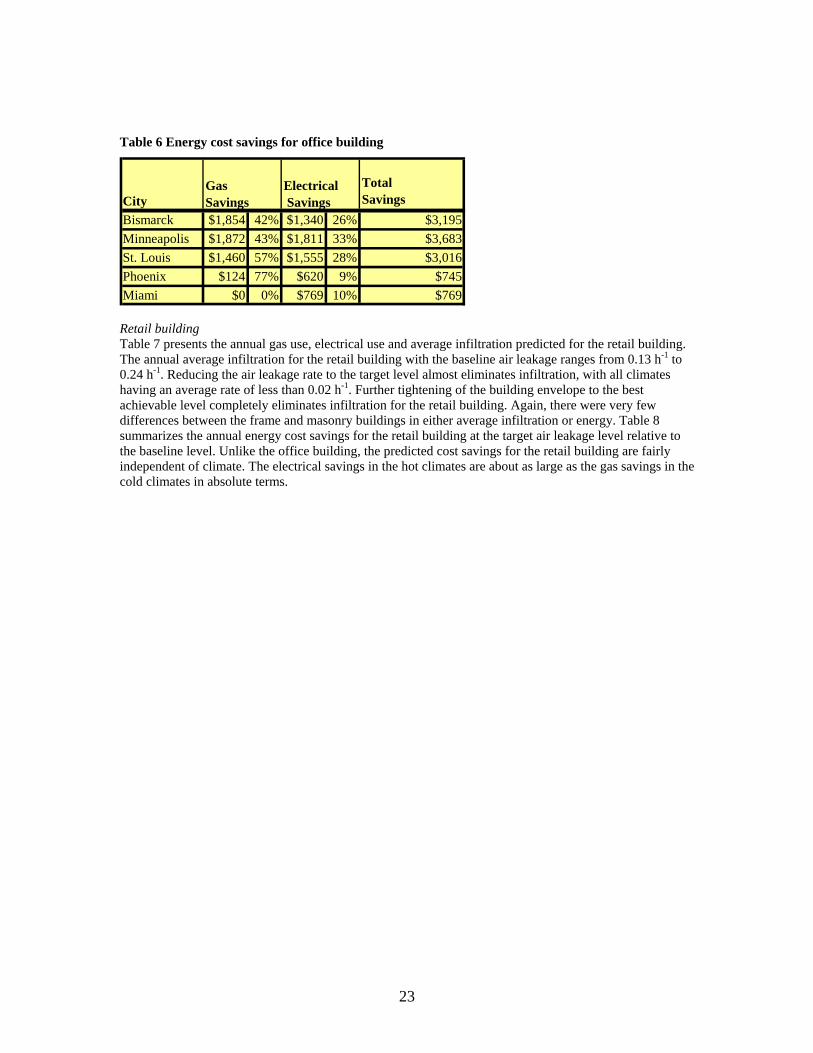
Table 6 Energy cost savings for office building

Retail building Table 7 presents the annual gas use, electrical use and average infiltration predicted for the retail building. The annual average infiltration for the retail building with the baseline air leakage ranges from 0.13 h-1 to 0.24 h-1. Reducing the air leakage rate to the target level almost eliminates infiltration, with all climates having an average rate of less than 0.02 h-1. Further tightening of the building envelope to the best achievable level completely eliminates infiltration for the retail building. Again, there were very few differences between the frame and masonry buildings in either average infiltration or energy. Table 8 summarizes the annual energy cost savings for the retail building at the target air leakage level relative to the baseline level. Unlike the office building, the predicted cost savings for the retail building are fairly independent of climate. The electrical savings in the hot climates are about as large as the gas savings in the cold climates in absolute terms.

CityTotal Savings

Bismarck $1,854 42% $1,340 26% $3,195Minneapolis $1,872 43% $1,811 33% $3,683St. Louis $1,460 57% $1,555 28% $3,016Phoenix $124 77% $620 9% $745Miami $0 0% $769 10% $769

Electrical Savings

GasSavings

23

24

Table 7 Annual gas use, electrical use and annual average infiltration for retail building

RetailSI UnitsBismarck Frame Building Masonry Building

Baseline Target Best Baseline Target BestAnnual Gas (kJ) 7.4E+08 5.5E+08 5.3E+08 7.4E+08 5.5E+08 5.3E+08Annual Electricity (kJ) 7.9E+07 7.7E+07 7.8E+07 7.8E+07 7.7E+07 7.7E+07Annual Average Infiltration (h-1) 0.20 0.02 0.00 0.20 0.02 0.00Minneapolis Frame Building Masonry Building

Baseline Target Best Baseline Target Best

stE+08

8

Baseline Target Best Baseline Target BestAnnual Gas (kJ) 2.9E+07 1.0E+07 1.0E+07 3.2E+07 1.3E+07 1.3E+07Annual Electricity (kJ) 3.1E+08 2.6E+08 2.6E+08 3.1E+08 2.7E+08 2.7E+08Annual Average Infiltration (h-1) 0.13 0.00 0.00 0.13 0.00 0.00Miami Frame Building Masonry Building


Annual Average Infiltration (h-1) 0.21 0.01 0.00 0.21 0.01 0.00IP UnitsBismarck Frame Building Masonry Building

Baseline Target Best Baseline Target BestAnnual Gas (Btu) 7.0E+08 5.2E+08 5.0E+08 7.0E+08 5.2E+08 5.0E+08Annual Electricity (Btu) 7.5E+07 7.3E+07 7.4E+07 7.4E+07 7.3E+07 7.3E+07Annual Average Infiltration (h-1) 0.20 0.02 0.00 0.20 0.02 0.00Minneapolis Frame Building Masonry Building

Baseline Target Best Baseline Target BestAnnual Gas (Btu) 6.7E+08 4.8E+08 4.6E+08 6.7E+08 4.8E+08 4.6E+08Annual Electricity (Btu) 8.2E+07 6.7E+07 6.3E+07 8.1E+07 6.6E+07 6.2E+07Annual Average Infiltration (h-1) 0.22 0.02 0.00 0.22 0.02 0.00St. Louis Frame Building Masonry Building

Baseline Target Best Baseline Target BestAnnual Gas (Btu) 3.8E+08 2.3E+08 2.2E+08 3.8E+08 2.4E+08 2.3E+08Annual Electricity (Btu) 1.4E+08 1.3E+08 1.3E+08 1.4E+08 1.3E+08 1.3E+08Annual Average Infiltration (h-1) 0.24 0.01 0.00 0.24 0.01 0.00Phoenix Frame Building Masonry Building

Baseline Target Best Baseline Target BestAnnual Gas (Btu) 2.7E+07 9.9E+06 9.8E+06 3.0E+07 1.2E+07 1.2E+07Annual Electricity (Btu) 2.9E+08 2.5E+08 2.5E+08 2.9E+08 2.5E+08 2.5E+08Annual Average Infiltration (h-1) 0.13 0.00 0.00 0.13 0.00 0.00Miami Frame Building Masonry Building

Baseline Target Best Baseline Target BestAnnual Gas (Btu) 6.6E+05 1.5E+04 1.5E+04 4.8E+05 0.0E+00 0.0E+00Annual Electricity (Btu) 3.5E+08 3.0E+08 3.0E+08 3.5E+08 3.0E+08 3.0E+08Annual Average Infiltration (h-1) 0.21 0.01 0.00 0.21 0.01 0.00

Annual Gas (kJ) 7.1E+08 5.1E+08 4.9E+08 7.1E+08 5.1E+08 4.9E+08Annual Electricity (kJ) 8.6E+07 7.0E+07 6.7E+07 8.6E+07 7.0E+07 6.6E+07Annual Average Infiltration (h-1) 0.22 0.02 0.00 0.22 0.02 0.00St. Louis Frame Building Masonry Building

Baseline Target Best Baseline Target BeAnnual Gas (kJ) 4.0E+08 2.5E+08 2.4E+08 4.0E+08 2.5E+08 2.4Annual Electricity (kJ) 1.5E+08 1.4E+08 1.4E+08 1.5E+08 1.4E+08 1.4E+0Annual Average Infiltration (h-1) 0.24 0.01 0.00 0.24 0.01 0.00Phoenix Frame Building Masonry Building

Table 8 Energy cost savings for retail building

Residential building Table 9 presents the annual gas use, electrical use and average infiltration predicted for the apartment building. The annual average infiltration rate for the apartment building with the baseline air leakage ranges is slightly higher than the other buildings and ranges from 0.19 h-1 to 0.26 h-1. Reducing the air leakage to the target level results in an average reduction in infiltration of 64 %. Further tightening of the building envelope to the best achievable level further reduces the infiltration by an average of 33 %. The infiltration remains higher in the tighter apartment buildings relative to the other buildings due to the lack of a mechanical system pressurization effect. The clapboard siding and masonry veneer buildings were quite similar with the masonry building resulting in slightly lower gas use. Table 10 summarizes the annual energy cost savings for the apartment building at the target air leakage level relative to the baseline level. Similar to the office building, the predicted cost savings for the apartment building are largest in the cold climates with gas savings of 40 % or more.

CityTotal Savings

Bismarck $1,835 26% $33 2% $1,869Minneapolis $1,908 28% $364 18% $2,272St. Louis $1,450 38% $298 9% $1,748Phoenix $176 64% $992 14% $1,169Miami $6 98% $1,224 14% $1,231

Gas SavingsElectrical Savings

25

Table 9 Annual gas use, electrical use and annual average infiltration for apartment building

ApartmentSI UnitsBismarck Clapboard Building Masonry Building

Baseline Target Best Baseline Target BestAnnual Gas (kJ) 5.7E+08 3.5E+08 2.9E+08 5.6E+08 3.4E+08 2.8E+08Annual Electricity (kJ) 5.7E+07 6.2E+07 6.6E+07 5.7E+07 6.2E+07 6.6E+07Annual Average Infiltration (h-1) 0.22 0.09 0.06 0.22 0.09 0.06Minneapolis Clapboard Building Masonry Building

Baseline Target Best Baseline Target BestAnnual Gas (kJ) 5.7E+08 3.2E+08 2.8E+08 5.6E+08 3.2E+08 2.6E+08Annual Electricity (kJ) 5.3E+07 6.0E+07 6.2E+07 5.3E+07 6.0E+07 6.2E+07Annual Average Infiltration (h-1) 0.24 0.09 0.06 0.24 0.09 0.06St. Louis Clapboard Building Masonry Building

Baseline Target Best Baseline Target BestAnnual Gas (kJ) 3.3E+08 1.4E+08 1.2E+08 3.2E+08 1.4E+08 1.2E+08Annual Electricity (kJ) 8.7E+07 9.7E+07 1.0E+08 8.7E+07 9.7E+07 1.0E+08Annual Average Infiltration (h-1) 0.25 0.09 0.06 0.26 0.09 0.06Phoenix Clapboard Building Masonry Building

Baseline Target Best Baseline Target BestAnnual Gas (kJ) 2.2E+07 8.1E+06 8.4E+06 2.0E+07 6.6E+06 7.3E+06Annual Electricity (kJ) 1.9E+08 1.8E+08 1.9E+08 1.8E+08 1.8E+08 1.9E+08Annual Average Infiltration (h-1) 0.19 0.07 0.05 0.19 0.07 0.05Miami Clapboard Building Masonry Building


Annual Average Infiltration (h-1) 0.26 0.08 0.05 0.26 0.08 0.05IP UnitsBismarck Clapboard Building Masonry Building

Baseline Target Best Baseline Target BestAnnual Gas (Btu) 5.4E+08 3.3E+08 2.7E+08 5.3E+08 3.2E+08 2.7E+08Annual Electricity (Btu) 5.4E+07 5.9E+07 6.2E+07 5.4E+07 5.9E+07 6.2E+07Annual Average Infiltration (h-1) 0.22 0.09 0.06 0.22 0.09 0.06Minneapolis Clapboard Building Masonry Building

Baseline Target Best Baseline Target BestAnnual Gas (Btu) 5.4E+08 3.0E+08 2.6E+08 5.3E+08 3.1E+08 2.4E+08Annual Electricity (Btu) 5.0E+07 5.7E+07 5.9E+07 5.0E+07 5.7E+07 5.9E+07Annual Average Infiltration (h-1) 0.24 0.09 0.06 0.24 0.09 0.06St. Louis Clapboard Building Masonry Building

Baseline Target Best Baseline Target BestAnnual Gas (Btu) 3.1E+08 1.4E+08 1.2E+08 3.1E+08 1.3E+08 1.1E+08Annual Electricity (Btu) 8.3E+07 9.2E+07 9.5E+07 8.2E+07 9.2E+07 9.5E+07Annual Average Infiltration (h-1) 0.25 0.09 0.06 0.26 0.09 0.06Phoenix Clapboard Building Masonry Building

Baseline Target Best Baseline Target BestAnnual Gas (Btu) 2.1E+07 7.6E+06 8.0E+06 1.9E+07 6.2E+06 6.9E+06Annual Electricity (Btu) 1.8E+08 1.8E+08 1.8E+08 1.7E+08 1.7E+08 1.8E+08Annual Average Infiltration (h-1) 0.19 0.07 0.05 0.19 0.07 0.05Miami Clapboard Building Masonry Building

Baseline Target Best Baseline Target Bestnnual Gas (Btu) 5.0E+06 1.9E+06 1.9E+06 4.6E+06 1.6E+06 1.6E+06nnual Electricity (Btu) 1.8E+08 1.7E+08 1.6E+08 1.8E+08 1.7E+08 1.6E+08nnual Average Infiltration (h-1) 0.26 0.08 0.05 0.26 0.08 0.05

AAA

26

apartment building cooling setpoints

urs al

cooling

would open windows for the free cooling. Figure 12 demonstrates this effect for the apartment building in Phoenix. The tighter target air leakage level results in predicted increases in cooling energy use from October through April but reduces cooling energy in the hottest months of June through September. The average savings during these hot months is 10 %.

Table 10 Energy cost savings for apartment building

Unlike the retail and o

CityTotal Savings

Bismarck $2,187 40% -$116 -9% $2,071Minneapolis $2,421 43% -$165 -14% $2,256St. Louis $1,794 57% -$232 -12% $1,562

$133$411

Gas Savin

Phoenix $133 65% $0 0%Miami $31 63% $380 9%

gsElectrical Savings

ffice buildings, tightening the residential building envelope in the cooler climates resulted in a predicted electrical cost penalty of up to 14 %. In all of the building types, there are some hours where the reduction of infiltration eliminates a ‘free cooling’ effect during which time the cool outdoor air offsets the internal heat gain of the building. However, in the apartment building for these cooler climates, this impact summed over the course of the year more than offsets the impact of lower infiltration during hot hours when it adds to the cooling load. There are key differences between the building types that produce this effect. First, the apartment building lacks both an economizer to purposefully take advantage of free cooling effect. In fact, the apartment also lacks continuous ventilationto coincidentally take advantage of the free cooling effect. Second, theare higher during the day and lower at night, which results in smaller cooling loads during the hottest hoand larger cooling hours during the cooler hours. However, it is likely that some of the predicted electricuse for cooling in the residential building would not occur in the real world because part of the freeeffect happens during winter or shoulder seasons when residents may not operate their air-conditioning and

27

0.0E+00

5.0E+06

1.0E+07

1.5E+07

2.0E+07

2.5E+07

3.0E+07

3.5E+07

Jan Feb Mar Apr May Jun Jul Aug Sep Oct Nov Dec

Mon

thly

ele

ctric

al u

se (k

J)

BaselineTarget

28

Figure 12 Monthly electrical use in Phoenix apartment building

Comparison to CBECS-derived benchmarks Since these prototype buildings are not based on an actual building, it is not possible to directly validate the model predictions. However, it is valuable to compare the predictions to available benchmarks of heating and cooling energy use in comparable U.S. buildings. One option is to compare the predicted annual gas and electricity use to recent Commercial Building Energy Consumption Survey (CBECS) results available from the U.S. Department of Energy. The most recent available commercial energy data available are for 1999 (http://www.eia.doe.gov/emeu/cbecs/detailed_tables_1999.html). The CBECS does not directly measure the portion of energy used in buildings for heating and cooling, but instead uses statistical methods to derive estimates of energy end-use consumption. For the 1999 CBECS, a new nonlinear regression method was used to estimate the total energy used, with a breakdown by principal building activity. To compare the results from this study, the results for the three baseline buildings were normalized by floorspace area. Similarly, the aggregate energy end-use data for the Office and Retail (Other than Mall) categories were normalized by the closest available floorspace numbers from the 1999 CBECS Building Characteristics tables. The 1999 CBECS value for natural gas used for space heating was normalized by total floorspace area in buildings with gas heating, the value for electricity used for cooling was normalized by total floorspace with cooling, and the value for ventilation was normalized by the total floorspace. CBECS also includes a small amount of electricity used for space heating but this amount was neglected. The normalized values of electricity used for cooling and electricity were then added to obtain the total electricity used for space conditioning. The values derived from the 1999 CBECS data are presented in Table 11. Note that these values vary considerably from the Commercial Buildings Energy End-Use Intensities listed in the 2004 Buildings Energy Databook (DOE 2004). One cause of the difference is that the Buildings Energy Databook uses older CBECS data from 1995. More significantly, the 1995 CBECS data is based on the discontinued methodology. As explained on the DOE Energy Information Agency website

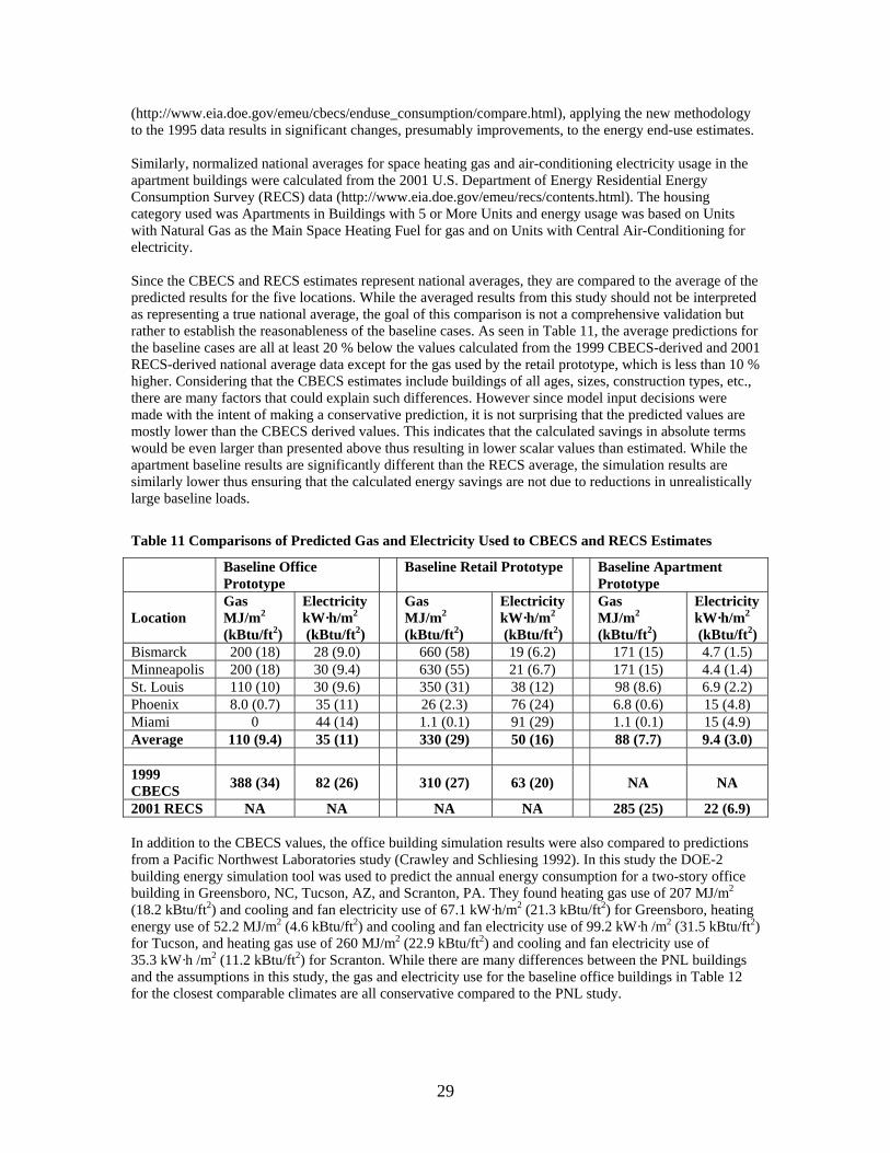
(http://www.eia.doe.gov/emeu/cbecs/enduse_consumption/compare.html), applying the new methodology to the 1995 data results in significant changes, presumably improvements, to the energy end-use estimates. Similarly, normalized national averages for space heating gas and air-conditioning electricity usage in the apartment buildings were calculated from the 2001 U.S. Department of Energy Residential Energy Consumption Survey (RECS) data (http://www.eia.doe.gov/emeu/recs/contents.html). The housing category used was Apartments in Buildings with 5 or More Units and energy usage was based on Units with Natural Gas as the Main Space Heating Fuel for gas and on Units with Central Air-Conditioning for electricity. Since the CBECS and RECS estimates represent national averages, they are compared to the average of the predicted results for the five locations. While the averaged results from this study should not be interpreted as representing a true national average, the goal of this comparison is not a comprehensive validation but rather to establish the reasonableness of the baseline cases. As seen in Table 11, the average predictions for the baseline cases are all at least 20 % below the values calculated from the 1999 CBECS-derived and 2001 RECS-derived national average data except for the gas used by the retail prototype, which is less than 10 % higher. Considering that the CBECS estimates include buildings of all ages, sizes, construction types, etc., there are many factors that could explain such differences. However since model input decisions were made with the intent of making a conservative prediction, it is not surprising that the predicted values are mostly lower than the CBECS derived values. This indicates that the calculated savings in absolute terms would be even larger than presented above thus resulting in lower scalar values than estimated. While the apartment baseline results are significantly different than the RECS average, the simulation results are similarly lower thus ensuring that the calculated energy savings are not due to reductions in unrealistically large baseline loads.

Table 11 Comparisons of Predicted Gas and Electricity Used to CBECS and RECS Estimates

Baseline Office Prototype

Baseline Retail Prototype Baseline Apartment Prototype

Location

Gas MJ/m2 (kBtu/ft2)

Electricity kW·h/m2 (kBtu/ft2)





Bismarck 200 (18) 28 (9.0) 660 (58) 19 (6.2) 171 (15) 4.7 (1.5) Minneapolis 200 (18) 30 (9.4) 630 (55) 21 (6.7) 171 (15) 4.4 (1.4) St. Louis 110 (10) 30 (9.6) 350 (31) 38 (12) 98 (8.6) 6.9 (2.2) Phoenix 8.0 (0.7) 35 (11) 26 (2.3) 76 (24) 6.8 (0.6) 15 (4.8) Miami 0 44 (14) 1.1 (0.1) 91 (29) 1.1 (0.1) 15 (4.9) Average 110 (9.4) 35 (11) 330 (29) 50 (16) 88 (7.7) 9.4 (3.0) 1999 CBECS 388 (34) 82 (26) 310 (27) 63 (20) NA NA

2001 RECS NA NA NA NA 285 (25) 22 (6.9) In addition to the CBECS values, the office building simulation results were also compared to predictions from a Pacific Northwest Laboratories study (Crawley and Schliesing 1992). In this study the DOE-2 building energy simulation tool was used to predict the annual energy consumption for a two-story office building in Greensboro, NC, Tucson, AZ, and Scranton, PA. They found heating gas use of 207 MJ/m2 (18.2 kBtu/ft2) and cooling and fan electricity use of 67.1 kW·h/m2 (21.3 kBtu/ft2) for Greensboro, heating energy use of 52.2 MJ/m2 (4.6 kBtu/ft2) and cooling and fan electricity use of 99.2 kW·h /m2 (31.5 kBtu/ft2) for Tucson, and heating gas use of 260 MJ/m2 (22.9 kBtu/ft2) and cooling and fan electricity use of 35.3 kW·h /m2 (11.2 kBtu/ft2) for Scranton. While there are many differences between the PNL buildings nd the assumptions in this study, the gas and electricity use for the baseline office buildings in Table 12 r the closest comparable climates are all conservative compared to the PNL study.

afo

29

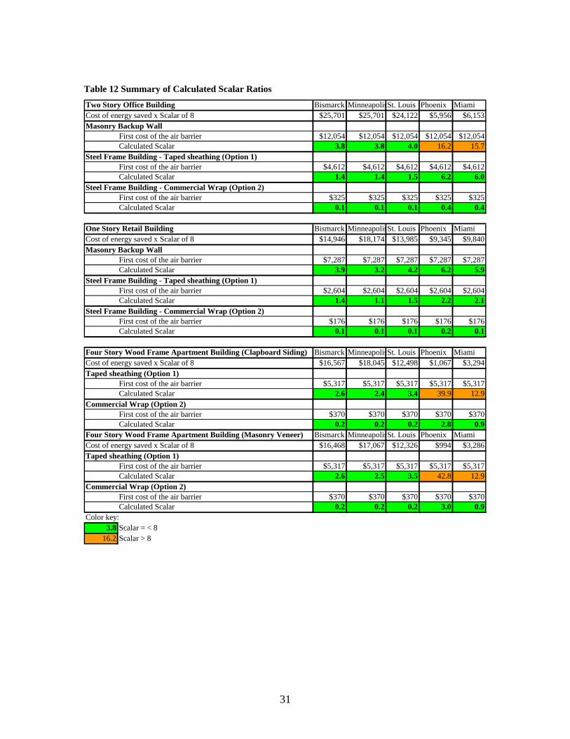
Cost Effectiveness As described earlier, a cost effectiveness analysis of the air barrier energy savings was conducted using the scalar ratio methodology employed by SSPC 90.1. This cost analysis was performed to put the calculated energy savings in context using estimated values of the costs associated with the air barrier measures. As seen in Table 12, the majority of cases with one exception (the office building with masonry backup in climate zones 1 and 2) have a Scalar Ratio less than 8 for the Target case. Based on this criterion, the residential building can use either of the airtightening options outlined in climate zones 3 and higher, but Option 2 is more cost effective in climate zones 1 and 2.

e continuous air barrier is cost-effective in climate 1 and 2, although significant, is not enough to

air

Office building: The masonry building expenditure on thzoned 3 and higher. The energy savings in climate zonesoffset the expenditure for the air barrier within the accepted guidelines of 90.1; in other words, with a Scalar of 16.2 or higher, it does not meet the maximum Scalar Ratio limit of 8. This would imply that anexception for masonry buildings in climate zones 1 and 2 is suggested by the study. The frame buildingbarrier is cost effective with both airtightening strategies in all climates. Retail building: The Scalar Ratio calculated for all the climate zones for both the masonry and frame building types indicate that all air barrier strategies are cost-effective. Multi-Unit Apartment Building: Based on the Scalar Ratio, the air barrier strategy option 1 is not cost-effective in climate zones 1 and 2, but the air barrier strategy option 2 is cost-effective in all climates. There is no significant difference between the building with clapboard siding and masonry veneer.

30

31

Table 12 Summary of Calculated Scalar Ratios

Two Story Office Building Bismarck MinneapolisSt. Louis Phoenix MiamiCost of energy saved x Scalar of 8 $25,701 $25,701 $24,122 $5,956 $6,153Masonry Backup Wall

First cost of the air barrier $12,054 $12,054 $12,054 $12,054 $12,054Calculated Scalar 3.8 3.8 4.0 16.2 15.7

Steel Frame Building - Taped sheathing (Option 1)First cost of the air barrier $4,612 $4,612 $4,612 $4,612 $4,612Calculated Scalar 1.4 1.4 1.5 6.2 6.0

Steel Frame Building - Commercial Wrap (Option 2)First cost of the air barrier $325 $325 $325 $325 $325Calculated Scalar 0.1 0.1 0.1 0.4 0.4

One Story Retail Building Bismarck MinneapolisSt. Louis Phoenix MiamiCost of energy saved x Scalar of 8 $14,946 $18,174 $13,985 $9,345 $9,840Masonry Backup Wall

First cost of the air barrier $7,287 $7,287 $7,287 $7,287 $7,287Calculated Scalar 3.9 3.2 4.2 6.2 5.9

Steel Frame Building - Taped sheathing (Option 1)First cost of the air barrier $2,604 $2,604 $2,604 $2,604 $2,604Calculated Scalar 1.4 1.1 1.5 2.2 2.1

Steel Frame Building - Commercial Wrap (Option 2)First cost of the air barrier $176 $176 $176 $176 $176Calculated Scalar 0.1 0.1 0.1 0.2 0.1

Four Story Wood Frame Apartment Building (Clapboard Siding) Bismarck MinneapolisSt. Louis Phoenix Miami$18,045 $12,498 $1,067 $3,294

$5,317 $5,317 $5,317 $5,317 $5,317

0

CoTa

st of energy saved x Scalar of 8 $16,567ped sheathing (Option 1)

First cost of the air barrier Calculated Scalar 2.6 2.4 3.4 39.9 12.9

Commercial Wrap (Option 2)First cost of the air barrier $370 $370 $370 $370 $37Calculated Scalar 0.2 0.2 0.2 2.8 0.9

Four Story Wood Frame Apartment Building (Masonry Veneer) Bismarck MinneapolisSt. Louis Phoenix MiamiCost of energy saved x Scalar of 8 $16,468 $17,067 $12,326 $994 $Taped sheathing (Option 1)

First cost of the air barrier Calculated Scalar

3,286

$5,317 $5,317 $5,317 $5,317 $5,3172.6 2.5 3.5 42.8 12.9

Commercial Wrap (Option 2)First cost of the air barrier $370 $370 $370 $370 $370Calculated Scalar 0.2 0.2 0.2 3.0 0.9

Color key:3.8 Scalar = < 8

16.2 Scalar > 8

Sensitivity Analysis Although the energy and airflow models used for this study require many input values, two of the most important values in determining the potential cost effectiveness of the proposed air barrier requirements are

lues ilding

fm/ft2 at 0.3 in H2O). Scalar ratios were calculated using the predicted energy savings for each

aseline level relative to the same target as above (i.e., 1.2 L/s-m2 at 75 Pa (0.24 cfm/ft2 at 0.3 in H O)) and

the baseline and target whole building air leakage values. As seen in Appendix A, the existing air leakage measurement cover a large range of air leakage values. To investigate the impact of the particular vaused in the study, sensitivity analyses were performed on each of these values for the frame office buin St. Louis (the middle climate studied). First, the whole building air leakage rate used for the baseline case was varied in steps over the range of 2.8 L/s-m2 at 75 Pa to 9.0 L/s-m2 at 75 Pa (0.55 cfm/ft2 at 0.3 inH2O to 1.8 cb 2the costs for option 1 in Table 5. As expected, Figure 13 shows the scalar ratio dropping as the baseline leakage increases. In other words, the energy savings of a building at the target airtightness relative to a tighter baseline building is smaller than the energy savings at the target airtightness relative to a leakier baseline building. However, the figure shows that even if the baseline leakage were set far lower than the 9.1 L/s-m2 (1.8 cfm/ft2) assumed in this study for St. Louis, the resulting scalar ratio would still be below 8 for this building and climate combination. For example, if the baseline building leakage rate were set at 4.2 L/s-m2 (0.8 cfm/ft2), which is the average of U.S. office buildings measured in past NIST studies, then the calculated scalar ratio would be about 3.3.

6

7

8

0

1

2

3

4

.0 4.0 6 7.0 9.0

il ng A (L 5 P

Scal

ar R

atio

Depe scal on seli kage

rcise erformed in which the baseline air leakage rate was held s e val is study but the target air leakage value was varied over a range of 1.2 L/s-m2 at 75 Pa to 2.8 L/s-m2 at 75

used

5

0.0 1.0 2 3.0 5.0 .0 8.0 10.0

Whole Bu di ir Leakage Rate /s·m @ 72 a)

Figure 13 ndence of ar ratio ba ne air lea rate

A similar exe was p teady at th ue used inthPa (0.24 cfm/ft2 at 0.3 in H2O to 0.55 cfm/ft2 at 0.3 in H2O). As above, simulations were performed for the frame office building in St. Louis to estimate energy savings and the cost for option 1 in Table 5 were to calculate the scalar ratios. While the predicted scalar ratio does increase with the target air leakage rate, Figure 14 shows that the scalar ratio is relatively insensitive to the target air leakage rate over the range studied for this building and climate combination. Specifically, if the building with the air barrier is assumed to be 2.33 times as leaky as the target of 1.2 L/s-m2 at 75 Pa (0.24 cfm/ft2 at 0.3 in H2O) assumed in this study, the predicted scalar ratio increases by only 20 % and remains far below 8.

32

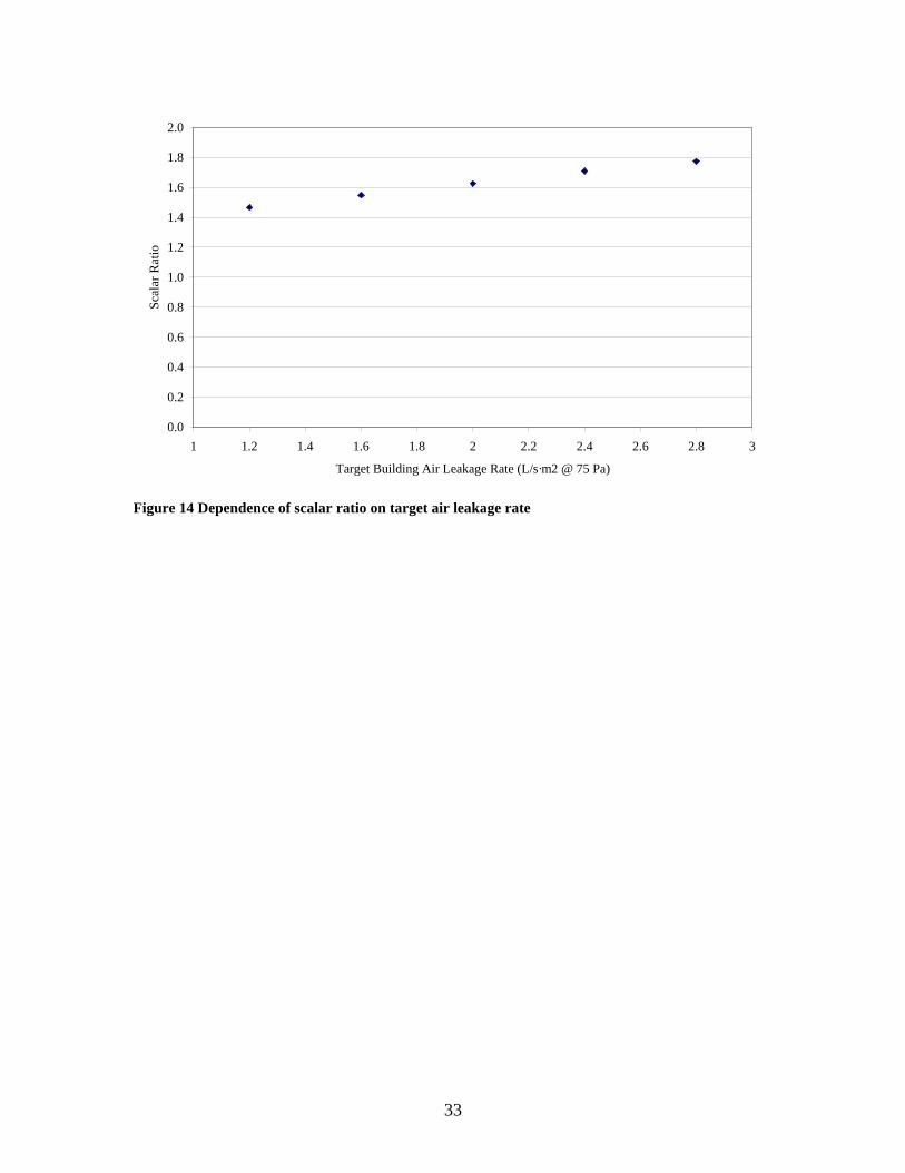
2.0

0.4

0.6

0.8

1.0

Scal

ar R

atio 1.2

1.4

1.6

1.8

0.0

0.2

1 1.2 1.4 1.6 1.8 2 2.2 2.4 2.6 2.8

Target Building Air Leakage Rate (L/s·m2 @ 75 Pa)

3

Figure 14 Dependence of scalar ratio on target air leakage rate

33

Discussion This simulation study included a small number of building types with a specific set of energy-related parameters (i.e., envelope construction types, internal loads, ventilation rates, etc.) in a limited set of climates. Predicted potential annual heating and energy cost savings for these buildings ranged from 2 % to 36 % with the largest savings occurring in the heating-dominated climates of Minneapolis and Bismarck and the smallest savings occurring in the cooling-dominated climates of Phoenix and Miami. The cost effectiveness analysis utilized costs for certain specific materials but other materials may be used to achieve the whole building airtightness target level used in the study. Only a few other reports of the energy impacts of infiltration in commercial buildings and the potential savings due to tightening could be found for comparison. For the most part, these other studies are not as detailed as the current effort and may employ building configuration, airtightness, and other parameters that vary significantly from this study but they do provide some reference for comparison. Potter et al. (1995) estimated the heating load due to infiltration for two U.K. office buildings of approximately equal size. They found that a 63 % reduction in air leakage could result in a reduction in annual heating energy loss due to infiltration of about 300 MW/m2. Since whole building energy analysis was not performed, this is not directly equivalent to the heating energy savings predicted in this study but it does concur with the potential large impact of building airtightness on heating energy use. Edwards (1999) reported a modeling study of the ventilation and infiltration energy impacts in a 10-story apartment building in a range of Canadian climates. This study employed the CONTAM multizone airflow model to create a model of an actual tested building and estimated that infiltration would be responsible for 31 % to 46 % of the average peak heating load (based on measurements in four Toronto apartment buildings reported by Scanada 1991). While the potential savings due to envelope tightening of 40 % to 43 % calculated for Bismarck and Minneapolis predicted in the current study are not directly comparable, the impact of infiltration on heating loads are of a similar magnitude. The Scanada report estimated that infiltration contributed an average of 32 % of the annual heating load in those buildings. Building Sciences LTD presents an estimate of potential annual heating savings for an industrial building in London of 60 MJ/m2 due to a reduction in envelope leakiness of 75 % (http://www.air-leakage.co.uk/why.htm). The gas savings for the target level relative to the baseline level in St. Louis (the closest climate) estimated in this study ranged from 56 MJ/m2 to 130 MJ/m2 depending on the building type. Again, these estimates are for different buildings with different assumptions but the magnitude of savings falls within the same overall range. Parekh (1992) described measured airtightness and monitored energy before and after sealing efforts in two existing high-rise residential buildings in Canada. The air leakage of the buildings was reduced by an average of 35 %, which resulted in an average heating energy consumption reduction of 9 %. While the energy saving is smaller than predicted in this study, the difference is readily explained by the modest reduction in air leakage achieved for this retrofit study. Similarly, Shaw and Reardon (1995) reported an 11 % reduction in monitored heating energy consumption after a 43 % improvement in measured airtightness of a 20-story office building in Ottawa. Again, the

in this study but the differences are easily explained duction in air leakage achieved in this retrofit study.

s mentioned above, this study included a limited set of building-climate combinations and this work could be extended in a variety of ways. Specific recommendations for future work include:

• Continue study to develop more refined (i.e., climate-specific) airtightness targets,

• Extend study to other building categories,

• Perform factorial analysis to examine the potential interaction between airtightness and other building parameters,

measured energy savings is smaller than the estimates by the different building type and the more modest re A

34

• Test airtightness of buildings built to a tightness standard (possibly in MA) to evaluate whether tightness targets are being met in practice,

• Analyze the costs and potential energy savings from tightening of existing buildings and develop recommendations for the existing building stock,

• And, develop diagnostic protocols and tools for failures of building envelopes that deteriorate IAQ and energy efficiency.

Acknowledgements This work was sponsored by the US. Department of Energy, Office of Building Technologies under Interagency Agreement No. DE-AI01-01EE27615. The authors wish to acknowledge the efforts of Terry Logee of DOE, Merle McBride and the ASHRAE SSPC90.1 Envelope Subcommittee in support of this project.

35

References Anis, W. 2001. “The Impact of Airtightness on System Design”, ASHRAE Journal Vol. 43, No. 12. Anon. 2002. "Monitored performance of an innovative multi-unit residential building" Canada Mortgage and Housing Corporation Research Highlight. Anon. 1998. “PROBE 14: Elizabeth Fry Building”, Building Services Journal, April 1998. Anon. 2003. “Learning curve”, Building Services Journal, September 2003. ASHRAE. 2001a. Ventilation for Acceptable Indoor Air Quality. ASHRAE Standard 62; American Society of Heating, Refrigerating and Air-Conditioning Engineers, Inc. ASHRAE. 2001b. Energy Standard for Buildings Except Low-Rise Residential Buildings. ASHRAE Standard 90.1; American Society of Heating, Refrigerating and Air-Conditioning Engineers, Inc. ASHRAE. 2001c. Handbook of Fundamentals. American Society of Heating, Refrigerating and Air-Conditioning Engineers, Inc. ASHRAE. 2001d. Energy-Efficient Design of Low-Rise Residential Buildings. ASHRAE Standard 90.2; American Society of Heating, Refrigerating and Air-Conditioning Engineers, Inc.

l. 45, No. 11.

STM. 1999. E779-99, Standard Test Method for Determining Air Leakage Rate by Fan Pressurization. American Society for Testing and Materials. Bombaru, Jutras, and Patenaude. 1988. “The Air Permeance of Building Materials”, Canada Mortgage and Housing Corporation. Briggs, R., Crawley, D., and J.S. Schliesing. 1992. Energy requirements for office buildings. Volume 1, Existing buildings. GRI-90/0236.1 by Battelle, Pacific Northwest Laboratory, for Gas Research Institute. CGSB. 1986. CAN/CGSB-149.10-86, Determination of the airtightness of building envelopes by the fan depressurization method using the building’s air handling systems. Canadian General Standards Board. CGSB. 1996. CAN/CGSB-149.15-96, Determination of the overall envelope airtightness of buildings by the fan depressurization method using the building’s air handling systems. Canadian General Standards Board. CIBSE. 2000. Technical Memoranda TM23:2000, Testing Buildings for Air Leakage. Chartered Institution of Building Services Engineers. Cohen, R. 2003. “Tightly knit.” Building Services Journal, June 2003. Crawley, D., and J. Schliesing. 1992. Energy requirements for office buildings. Volume 2, Recent and future buildings. GRI-90/0236.2 by Battelle, Pacific Northwest Laboratory, for Gas Research Institute. Diamond, R.C., Modera, M.P., and H.E. Feustel. 1986. "Ventilation and Occupant Behavior in Two Apartment Buildings," in, Proceedings, The 7th Air Infiltration Centre Conference on Occupant Interaction with Ventilation Systems, Stratford, UK. Dols, W.S. and G.W. Walton. 2002. CONTAMW 2.0 User Manual, NISTIR 6921.

Ask, A. 2003. “Ventilation and Air Leakage”, ASHRAE Journal Vo A

36

Edwards, C. 1999. Modelling of Ventilation and Infiltration Energy Impacts in Mid- and High-Rise

Bulfinch

E.

orida.

. Building Services Res ch Pros racteristics, Test Methods and Specifications for Large Buil g

Apartment Buildings. Report by Sheltair Scientific Ltd. For Canada Mortgage and Housing Corporation. Emmerich, S., Persily, A. and D. VanBronkhorst. 1995. A workplan to analyze the energy impacts of envelope airtightness in office buildings. NSITIR 5758, National Institute of Standards and Technology. Emmerich, S., and A. Persily. 1998. “Energy Impacts of Infiltration and Ventilation in U.S. Office Buildings Using Multizone Airflow Simulation.” IAQ and Energy ’98, American Society of Heating,

efrigerating, and Air-Conditioning Engineers, Inc. R Feustel, H.E. and R.C. Diamond. 1996. "Diagnostics and Measurements of Infiltration and Ventilation Systems in High-Rise Apartment Buildings", in Proceedings of the ACEEE Summer Study on Energy Efficiency in Buildings. HFG. 2004. Air Barrier Study. Hanscomb Faithful and Gould International, prepared for ShepleyRichardson and Abbott. ISO. 1996. Standard 9972, Thermal Insulation – Determination of Building Airtightness – Fan Pressurization Method. International Standards Organization. Kennett. 2004. “Relocation, relocation.” Building Services Journal, June 2004. Klein S. TRNSYS - A Transient System Simulation Program Engineering Experiment Station Report 38-13. (2000) Solar Energy Laboratory, University of Wisconsin - Madison. Marion,W. and K. Urban. 1995. User’s Manual for TMY2s. National Renewable Energy Laboratory. McBride, M.F. 1995. “Development of Economic Scalar Ratios for ASHRAE Standard 90.1R”,

roceedings of Thermal Performance of the Exterior Envelopes of Buildings VI, ASHRAP McDowell, T., Emmerich, S., Thornton, J., and G. Walton. 2003. “Integration of Airflow and Energy Simulation Using CONTAM and TRNSYS.” ASHRAE Transactions 2003. Modera, M.P., Brunsell, J.T. and R. C. Diamond. 1985. "Improving Diagnostics and Energy Analysis for Multifamily Buildings: A Case Study," in Proceedings, of the Thermal Performance of the

xterior Envelopes of Buildings, Clearwater, FlE Olivier, D. 2001. “Shattering the energy barrier” Building Services Journal: April 2001. Parekh, A. 1992 “Power Demand and Energy Savings Through Air Leakage Control in High-Rise Residential Buildings in Cold Climates”. 1992. Proceedings of Thermal Performance of the Exterior

nvelope of Buildings V. E Persily, A.K. 1993. Envelope Design Guidelines for Office Buildings: Thermal Integrity and Airtightness. NISTIR 4821, National Institute of Standards and Technology.

ersily, A.K. 1998. “Airtightness of Commercial and Institutional Buildings” Proceedings of ASHRAE PThermal Envelopes VII Conference. Potter, I., Jones, T., and W. Booth. 1995. TechNote 8/95 Air Leakage of Office Buildings

ear and Information Association.

kiw, G. and B. Phillips. 2001. Air Leakage Chadin s. Canada Mortgage and Housing Corporation research report.

37

Scan a ir Leakage , CMHC Final Report. Shaw, CSTP 125 Spinu, M

ynertech Systems Corporation. 1987. "Integrating Analytical Tactics into New York State's eatherization Assistance Program: Project Findings," Albany, New York: New York State Energy and

ity.

tional Institute of Standards and Technology. Wray, C., Theaker, I., and P. Moffatt. 1998. "Field Testing to Characterise Suite Ventilation in Recently Constructed Mid- and High-Rise Residential Buildings", CMHC Project Report.

ad . 1991. Development of Design Procedures and Guidelines for Reducing Electrical Demand by A Control in High-Rise Residential Buildings

. Y., and J. T. Reardon. 1995. “Changes in Airtightness Levels of Six Office Buildings” ASTM 5, American Society of Testing and Materials.

. 2004. E-mail to Wagdy Anis dated 06/18/2004.

SWResearch Development Author TWC. 2004. “Prototype Air Barrier Buildings” The Waterproofing Company, Boston, MA. Walton G. 1989. AIRNET - A Computer Program for Building Airflow Network Modeling. NISTIR 89-4072. Na

38

Appendix A Cable A1 summa

ommercial Building Airtightness Data rizes the measured whole building envelope airtightness data that was considered in

nalyzed by Persily (1998), however some additional buildings were added. The air leakage values in the

r ber of stories, or building floor area was not available for

Data

Building type Year of Construction Stories Floor area Air leakage

(0.3 in w.g.)

Ref

Tdeveloping the airtightness levels for this study. The majority of this data was previously reviewed andatable are normalized by the area of the above-ground portion of the building envelope. Information on yeaof construction, building construction type, numll buildings. a

Table A1 Summary Table of Measured Nonresidential Building Envelope Airtightness

Building

construction type at 75 Pa

m2 L/s-m2 cfm/ft2

Anchorage Office 1981 Concrete panel 6 48500 3.8 0.75 1

0.46 1 1977 Concrete panel 15 21600 3.4 0.67 1

Huron Office 1978 Masonry 4 6900 1.1 0.21 1 .80 1

00 2.0 0.39 1 5.2 1.03 1

100 12.0 2.37 7

92 3 22300 3.1 0.60 2 Admin School <1992 3 8200 2

7 2 B chool <1992 3 5600 1.8 0.36 2

0.17 2 .66 2

4.1 0.80 2 0.19 2 0.80 2

S. Pines School <1992 3 4400 1.0 0.19 2 2 2

4 2

1970 Concrete panel 9 6.2 1.23 3 7 3.1 0.61 3

1970 Concrete panel 20 2.6 0.61 3 0.67 3 0.39 3 0.39 3

3 3

1.77 4 NRCC-S-B School 1971 Masonry 1 1900 8.2 1.61 4 NRCC-S-C School 1965 Masonry 1 3800 7.4 1.45 4

Ann Arbor Office 1975 Masonry 4 5300 2.3 Columbia Office

Norfolk Office 1978 Masonry 8 18600 4.1 0Pittsfield Office 1977 Masonry 2 18

Springfield Office 1982 Concrete panel 5 14600 Overland Office 1990 Curtain 5 35

Albany School <19

0.7 0.15 Argentine School <1992 3 700 2.9 0.5ishop Ryan S

CLC School <1992 3 4600 0.9 Green Mtn. School <1992 3 2400 3.3 0

reen Gym School <1992 3 900 GLaurel School <1992 3 1500 1.0 Middle School <1992 3 7200 4.1

S. Tama School <1992 3 700 2.3 0.45Russell School <1992 3 3300 3.0 0.59Velva School <1992 3 5600 2.7 0.5

NRCC-A Office NRCC-B Office 1964 Concrete panel 1NRCC-C Office NRCC-D Office 1971 Curtain 20 3.4 NRCC-E Office 1968 Curtain 21 2.0 NRCC-F Office 1973 Concrete panel 16 2.0 NRCC-G Office 1974 Concrete panel 25 2.8 0.55NRCC-H Office 1974 Curtain 20 1.4 0.27

NRCC-S-A School 1970 Concrete panel 1 2700 9.0

39

NRCC-S-D School 1973 Masonry 1 3500 12.3 NRCC-S-E School 1957 Masonry 1 3700 7.1 1

2.41 4 .41 4

1.25 4 4 4

2.25 4 1.65 4

3200 5.5 1.09 4

1.77 5 1.37 5

tail 1978 Masonry 3 19.8 3.90 5 2 5 5 5

tail 1955 Masonry 3 17.0 3.34 5 7.4 3.42 5

anel 3 14.1 2.77 5 RCC-RM Retail 1957 Masonry 3 5.7 1.13 5

19.4 3.82 5

2.4 0.47 14

0.41 14

ent 1981 Masonry 5 4.9 0.96 6

3.1 0.61 10BRE-2 Office 1963 Masonry 0.59 10

0.61 10 6.7 1.32 10

3.8 0.75 101.01 101.71 10

BRE-8 Office 1971 Concrete panel 9.5 1.88 1010.2 2.00 10

BRE-10 Office 1985 Concrete panel 11.6 2.28 10

0.72 13V Elizabethan Masonry 3 4.3 0.83 13

0.8513

w/ 2 2.14

13

panels on .07

13

masonry 8.5 1.6713

.8413

wall/brick 4.3 0.8513

NRCC-S-F School 1952 Masonry 1 3100 6.3 NRCC-S-G School 1968 Masonry 1 5400 5.9 1.17 NRCC-S-H School 1965 Masonry 1 5200 4.9 0.96 NRCC-S-I School 1968 Masonry 1 2600 11.4NRCC-S-J School 1972 Masonry 1 3000 8.4 NRCC-S-K School 1968 Masonry 1

NRCC-BH Retail 1957 Masonry 3 9.0 NRCC-CK Retail 1963 Masonry 3 6.9 NRCC-HC ReNRCC-MD Retail 1977 Masonry 3 18.4 3.6NRCC-MK Retail 1967 Masonry 3 9.4 1.8

RCC-MS ReNNRCC-OD Retail 1979 Concrete panel 3 1NRCC-PO Retail 1979 Concrete pNNRCC-WG Retail 1954 Masonry 3

Parekh1 Apartment <1992 21

Parekh2 Apartment <1992 10 2.1 NRCC-R Apartm

BRE-1 Office 1980 Masonry

3.0BRE-3 Office 1991 Masonry 3.1BRE-4 Office 1965 Masonry BRE-5 Office 1987 Masonry BRE-6 Office 1990 Masonry 5.1

asonry 8.7BRE-7 Office 1990 M

BRE-9 Office 1986 Masonry

BSRIA-1 OfficeNV 1970 Prefab panels 2 3.7BSRIA-2 OfficeNBSRIA-3 Office 1991 Steelframe w/

masonry 6

4.4BSRIA-4 Office 1987.5 Steelframe

masonry 10.9BSRIA-5 OfficeNV 1963 Concrete 7

frame 5.4 1BSRIA-6 Office 1991 Steelframe w/ 3

BSRIA-7 Office 1986 Steelframe w/ masonry

6 14.5 2

BSRIA-8 Office 1989 Curtain 5

40

BSRIA-9 Office 1991 Steelframe w/ masonry

2 6.9 1.36

13

SRIA-10 Office 1990 Steelframe w/ 3 1.22

13

elframe w/ masonry

3 11.8 2.31

13

ame w/ masonry

3 13.5 2.64

13

0.52 11

<1999 Curtain 64 270000 2.8 0.55 11

0.32 9 1.55 9

3 Healthcare 1992 Masonry 1 260 13.2 2.59 9 0.61 9

310 10.9 2.15 9 6 Office 1961 Masonry 2 1180 3.2 0.62 9 7 School 1968 Masonry 1 1570 7.8 1.54 9 8 Office 1981 Masonry/frame 1 80 12.3 2.43 9 9 Healthcare 1959 Masonry 1 140 7.4 1.45 9

10 Office 1986 Masonry 1 570 7.5 1.47 9 11 Industrial 1960 Masonry/metal 1 170 15.2 3.00 9 12 Sports 1987 Masonry 1 1550 6.4 1.27 9 13 Daycare 1970 Masonry 1 240 17.3 3.40 9 14 School 1990 Manufactured 1 160 4.2 0.82 9 15 Healthcare 1986 Masonry 1 190 6.4 1.25 9 16 Office 1988 Manufactured 1 460 4.3 0.84 9 17 School 1975 Masonry 1 1550 5.5 1.08 9 18 Assembly 1986 Masonry 2 2090 3.6 0.71 9 19 Restaurant 1975 Frame/masonry 1 180 7.7 1.52 9 20 Office 1969 Masonry 1 270 3.8 0.76 9 21 Healthcare 1987 Frame 1 240 12.0 2.36 9 22 Restaurant 1994 Masonry 1 330 2.5 0.49 9 23 Industrial 1984 Metal 1 280 14.0 2.75 9 24 Library 1989 Masonry 1 800 1.2 0.24 9 25 Sports 1987 Masonry 1 250 17.0 3.34 9 26 Office 1994 Frame 1 90 19.7 3.87 9 27 Office 1994 Frame 1 90 19.5 3.84 9 28 Industrial 1994 Frame 1 180 13.5 2.66 9 29 Office 1983 Manufactured 1 470 15.1 2.96 9 30 Industrial 1941 Frame 2 300 27.0 5.31 9 31 Restaurant 1986 Masonry 1 220 9.6 1.88 9 32 Restaurant 1994 Frame 1 400 7.9 1.56 9 33 Restaurant 1994 Masonry 1 290 8.2 1.62 9 34 Office 1931 Frame/masonry 1 170 11.5 2.25 9 35 Restaurant 1986 Masonry 1 310 4.4 0.86 9 36 Industrial 1966 Masonry 1 1500 3.5 0.69 9 37 Office 1972 Masonry 1 170 4.5 0.89 9 38 Office 1972 Masonry 1 370 3.4 0.67 9

Bmasonry 6.2

BSRIA-11 OfficeNV 1992 Ste

BSRIA-12 Office 1992 Steelfr

PSU-1 Library <1999 Curtain 6 12077 2.6PSU-2 Office

Florida

1 Office 1965 Masonry 1 500 1.6 2 Assembly 1965 Masonry 1 460 7.9

4 Assembly 1970 Masonry/frame 2 980 3.1 5 Assembly 1959 Masonry 1

41

39 Office 1946 Masonry 1 200 9.6 1.89 9 2.95 9 2.32 9

.91 9 8 9

.44 9 Industrial 1966 Frame/masonry 1 240 12.5 2.46 9

6.81 9 47 Sports 1966 Frame/masonry 1 90 12.7 2.51 9

50 Retail nry 1 90 20.8 0 9 51 Office 1951 Masonry 1 500 9 52 Office 1964 Masonry 1 9 53 Industrial 1986 M al 260 3.5 0.69 9

1 I I

R t 6 Of ce 1990 Masonry 620 2.1 0.40

Masonry Masonry Masonry Masonry Masonry Masonry Masonry

ELEM. SCHOOL 1

40 School 1966 Frame/masonry 1 230 15.0 41 Animal 1966 Frame/masonry 1 70 11.8 42 Office 1966 Frame/masonry 1 590 14.8 243 Bar 1966 Frame/masonry 1 200 20.7 4.044 Office 1966 Frame/masonry 1 120 17.5 345 46 Office 1966 Frame/masonry 1 350 34.6

49 Retail 1966 1966 Fram

Frame/masonrye/maso

1 90 8.9 1.754.1

6.6 1.30

9

170 3.4 0.66 et 1

54 Office 1976 Masonry 1 240 18.6

.6 2.29 1.69

9 55 ndustrial 1978 Metal 1 930 9 56 ndustrial 1983 Metal 1 1150 5.6 1.10 9 57 Sports 1982 Masonry 1 660 15.3

3.3 3.00 0.64

9 58 Retail 1994 Masonry 1 430 9 59 Retail 1973 Masonry 1 150 9.9 1.95 9 60 Office 1985 Manufactured

Ma ed1 80 4.3 0.86 9

61 6

Office esta ran

1983 19 3

nufacturFrame

1 1

120 730

9.0 5.3

1.78 1.04

9 9 2

3u

fi6

1 9 64 School 1965 1 940 3.1 0.61 9 65 School 1965 1 190 3.0 0.59 9 66 School 1965 1 470 9.1 1.79 9 67 Hotel 1977 1 1400 6.7 1.32 9 68 Hotel 1977 2 1180 6.3 1.24 9 69 Retail 1989 1 400 10.9 2.16 9 70 Retail 1969 1 230 1.1 0.22 9

FSEC2 1 1966 MAS NRY 4

CHIC ST. O 1 657.9 40.0 7.85 12

2 KEN RE 1993 MASONRY 2COMMUNITY ENTE

1 93.66 3.7 0.73 123 C R 1991 MET/FRAME 2223.5 1

ELEM. SCHOOL 2 1 01.6 19.93 12

4 1998 MET/MAS ELEM. SCHOOL 3

1 464.5 41.8 8.21 125 1998 MET/MAS

REST. 1 464.5 46.5 9.13 12

6 SEAFOOD 1998 FRAME 762.15 28.2 5.54 1RIVER FRONT REST.

1 27 1986 MASONRY 2 543.47

STEAK REST. 3.8 0.74 12

8 HOUSE 1995 MET/FRAME 1 568.08 MDL. SCHOOL 1 B

29.1 5.70 129 1996 FRAME 1 65.587

MDL. SCHOOL 1 SW 6.1 1.20 12

10 1991 FRAME 1 60.385 MDL. SCHOOL 1 D

3.9 0.77 1211 1991 FRAME 1 70.232

MDL. SCHOOL 1 E 5.3 1.05 12

12 1991 FRAME 1 70.232 MDL. SCHOOL 2 1

11.6 2.27 1213 1997 FRAME 1 66.888

MDL. SCHOOL 2 6 12.0 2.36 12

14 1997 FRAME 1 66.888 15 MDL. SCHOOL 2 7

13.9 2.72 121997 FRAME 66.888 19.9 3.89 1

16 BAR AND GRILL 1 2

1985 MASONRY 1 222.96 9.5 1.87 12CONVEN. STORE

17 1988 MASONRY 1 4

OCEAN FRONT REST. 01.33 10.1 1.98 12

18 1962 FRAME 1 555.26 27.3 5.36 12

42

19 GREEK REST. 1960 M 1CHAR FICE

ASONRY 1 39.35 35.7 6.99 1220 ITY OF 1984 MET/MAS 3

O l parame orted fo uildi

s for Me Airtightn ta A.K. and ot. 1986. "Pr tion Fede Buildi easured

uildings STP 904, H schse agu ds., Am Society Tests, Philadel

, T., Turn Fisher, G., T on, B. gman. 1992. "Fan Pressurizat ings," Th erformance xteri es of ildings V, ASHRAE, nta,

G.T. and aw. 1976. "Studies on Ex ll Air Tightness an Air Infiltr of TASHRAE ctions, Vol. pp. 1

.Y. and L 1979. "Air T ss and Air Infiltration of School Buildings," ASHRAE , Vol.85, pp. 85-95.

.Y. 1981. ghtness: Sup ets an g Ma AE Journal, 198pp.44-46 6. .Y., Ma ousseau. 1991. "Overal and Com Airtightness Valu a FiS tment B RAE Tr ns, Vol.97, Part 2, pp.347-353.

7. Persi , A.K., Dol nger, S.J. and S. Kirchner. 1991. "Preliminary R sults of theE ental Evalu the Federal R s Cent land M ssouri," NISTIR 4634. 8 n, L.I. 1986 akage in Ind Build cripti pm ," MeasuredLeakage of Buildings, ASTM STP 904, H schse agus Eds., Ame ety for Testinga als, Philad p. 101-105. 9 ings, J.B., W C.R., Moyer, N., Fairey, cKendry. 1996. ncontrolled Ai ow in sidential Bu -CR-878-96, Flori ergy enter. 10. Perera, M.D.A.E. erson, J., an e le Air Leakage Predictor for O B ng e Airtightness During re R furbishment. CIBSE NatConference.

.P., Yuill, G.K. and B.W 999 Fi Testing o Tall BuildingsEnvelop ge Rate Tra Vol. (2).

12. Cummings, J.B., Shirey, D.B., Withers, C., Raustad . Moyer. 2000. Evaluating the Impacts ofPerfo ro ommercial and Institutional

Buildings, Final Report, FSEC-CR-1210-00.

13. Potter, I., Jones, T., and W. Booth. 1995. TechNote eakage of Office Buildings. Building Services Research and Information Association.

14. Parekh, A. 1992. 'Power Demand and Energy Savings Through Air Leakage C rol in High-R Buildings Climates'. P ing rformance of the Exterior Envelope of

Buildings V.

1 47.54 19.9 3.91 12verall mean 9.7 1.9 Note: Not al ters were rep r some b ngs. Reference asured ess Da1. Persily, R.A. Gr essuriza Testing of ral ngs," M Air Leakage of Band Material

, ASTMph a, pp. 184-200.

.R. Tre l and P.L. L s, E erican for ing i

2. Brennan er, W., homps , and B. Li ion ofSchool Build ermal P of the E or Envelop Bu Atla pp. 643-645. 3. Tamura, C.Y. Sh terior Wa d ation all Buildings," Transa 82 (II), 22-34. 4. Shaw, C . Jones. ightneTransactions Part 1, 5. Shaw. C "Air Ti ermark d Shoppin lls," ASHR March 1,

Shaw, Ctory Apar

gee R.J. and J. Ruilding," ASH

l ponent es of ve-ansactio

ly s, W.S., Nabi e

nvironm ation of ecord er in Over i

. Lundi . "Air Le ustrial ings - Des on of Equi ent Air .R. Tre l and P.L. L , rican Soci

nd Materi elphia, p

. Cumm ithers, P., and B. M U r Fl Non-Re ildings, FSEC da Solar En C

S., Hend d B.C. W bb p. 1997. Sim fficeuildings: Assessi Envelop Design or Befo e ional

11. Bahnfleth, W . Lee. 1 . "Protocol for eld f to Determine e Air Leaka ," ASHRAE nsactions, 105

, R. and N Uncontrolled Air Flow and HVAC rmance P blems on Florida's C

8/95 Air L

ont ise

Residential in Cold roceed s of Thermal Pe

43

Building Envelope Impact On HVAC Energy Use€¦ · · 2016-09-22Building Envelope Impact On HVAC...

Documents

Transcript of Building Envelope Impact On HVAC Energy Use€¦ · · 2016-09-22Building Envelope Impact On HVAC...