Budgeting Harmonics for ZigBee Front End Modules · Budgeting Harmonics for ZigBee Front End...
14
Budgeting Harmonics for ZigBee Front End Modules By Stephane Wloczysiak, Skyworks Solutions, Inc. Keywords ZigBee® Systems 2.4 GHz IEEE Std 802.15.4TM-2003 Standard Front-end Module Regulatory Standard Emission Requirements Harmonics Spurious Envelope Detector Introduction The growth of low power, cost effective wireless systems is driving more applications to use ZigBee protocol. While for some of them, the signal needs to propagate over a short range, when covering a large building or operating outdoor over a wide range for example, the system may benefit from transmitting more power. Actually [1] shows that a ZigBee radio system powered by a 20dBm power amplifier (PA) significantly increases its range compared to a low power 0dBm by 400% from 133 to 543 meters. However, adding a transmit PA may generate higher spurious, in particular -- the harmonic spurs. And additional filtering is required to satisfy radiated emission requirement of the different regulatory standards listed in Table 1. This document details how to specify harmonics for a ZigBee FEM. It reviews the requirements from the different regulatory standards, analyzes through simulation harmonics content of offset quadrature phase-shift keying (OQPSK) spread spectrum modulation and evaluates the effects of the measurement bandwidth and detector on the harmonics level of both sine and ZigBee waveforms. Finally, measurement data is provided to illustrate the simulations results.
Transcript of Budgeting Harmonics for ZigBee Front End Modules · Budgeting Harmonics for ZigBee Front End...

Budgeting Harmonics for ZigBee Front End Modules
By Stephane Wloczysiak, Skyworks Solutions, Inc.
Keywords ZigBee® Systems 2.4 GHz IEEE Std 802.15.4TM-2003 Standard Front-end Module Regulatory Standard Emission Requirements Harmonics Spurious Envelope Detector
Introduction The growth of low power, cost effective wireless systems is driving more applications to use ZigBee protocol. While for some of them, the signal needs to propagate over a short range, when covering a large building or operating outdoor over a wide range for example, the system may benefit from transmitting more power. Actually [1] shows that a ZigBee radio system powered by a 20dBm power amplifier (PA) significantly increases its range compared to a low power 0dBm by 400% from 133 to 543 meters. However, adding a transmit PA may generate higher spurious, in particular -- the harmonic spurs. And additional filtering is required to satisfy radiated emission requirement of the different regulatory standards listed in Table 1. This document details how to specify harmonics for a ZigBee FEM. It reviews the requirements from the different regulatory standards, analyzes through simulation harmonics content of offset quadrature phase-shift keying (OQPSK) spread spectrum modulation and evaluates the effects of the measurement bandwidth and detector on the harmonics level of both sine and ZigBee waveforms. Finally, measurement data is provided to illustrate the simulations results.
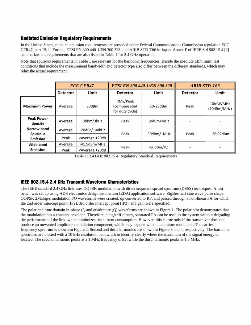
Radiated Emission Regulatory Requirements In the United States, radiated emission requirements are provided under Federal Communications Commission regulation FCC CFR47, part 15; in Europe, ETSI EN 300 440-1/EN 300 328; and ARIB STD-T66 in Japan. Annex F of IEEE Std 802.15.4 [2] summarizes the requirements that are also listed in Table 1 for 2.4 GHz operation. Note that spurious requirements in Table 1 are relevant for the harmonic frequencies. Beside the absolute dBm limit, test conditions that include the measurement bandwidth and detector type also differ between the different standards, which may relax the actual requirement.
FCC CFR47 ETSI EN 300 440-1/EN 300 328 ARIB STD-T66 Detector Limit Detector Limit Detector Limit
Maximum Power Average 30dBm RMS/Peak
(compensated for duty cycle)
20/23dBm Peak 10mW/MHz (10dBm/MHz)
Peak Power density
Average 8dBm/3kHz Peak 10dBm/MHz ‐ ‐
Narrow band Spurious Emission
Average ‐20dBc/100kHz Peak ‐30dBm/1MHz Peak ‐26.02dBm
Peak <Average +20dB
Wide band Emission
Average ‐41.5dBm/MHzPeak ‐80dBm/Hz ‐ ‐
Peak <Average +20dB
Table 1: 2.4 GHz 802.15.4 Regulatory Standard Requirements
IEEE 802.15.4 2.4 GHz Transmit Waveform Characteristics The IEEE standard 2.4 GHz link uses OQPSK modulation with direct sequence spread spectrum (DSSS) techniques. A test bench was set up using ADS electronics design automation (EDA) application software. ZigBee half sine wave pulse shape OQPSK 2Mchip/s modulation I/Q waveforms were created, up converted to RF, and passed through a non-linear PA for which the 2nd order intercept point (IP2), 3rd order intercept point (IP3), and gain were specified. The polar and time domain in-phase (I) and quadrature (Q) waveforms are shown in Figure 1. The polar plot demonstrates that the modulation has a constant envelope. Therefore, a high efficiency, saturated PA can be used in the system without degrading the performance of the link, which minimizes the current consumption. However, this is true only if the transceiver does not produce an unwanted amplitude modulation component, which may happen with a quadrature modulator. The carrier frequency spectrum is shown in Figure 2. Second and third harmonics are shown in Figure 3 and 4, respectively. The harmonic spectrums are plotted with a 10 kHz resolution bandwidth to identify clearly where the maximum of the signal energy is located. The second harmonic peaks at a 1 MHz frequency offset while the third harmonic peaks at 1.5 MHz.

Figure 1. ZigBee 2MChips/s OQPSK I/Q Constellation and Time Domain Waveforms
Figure 2. ZigBee 2MChips/s OQPSK Fundamental Spectrum
-0.833 -0.667 -0.500 -0.333 -0.167 0.000 0.167 0.333 0.500 0.667 0.833-1.000 1.000
-0.833
-0.667
-0.500
-0.333
-0.167
0.000
0.167
0.333
0.500
0.667
0.833
-1.000
1.000
I_OQPSK
Q_O
QPS
K
5.5 6.0 6.5 7.0 7.5 8.0 8.5 9.0 9.55.0 10.0
-1.0
-0.8
-0.6
-0.4
-0.2
0.0
0.2
0.4
0.6
0.8
1.0
-1.2
1.2
time, usec
Q_O
QP
SK,
VI_
OQ
PSK
, V m4 m5
m4time=I_OQPSK=-61.fV
5.0usecm5time=I_OQPSK=78.fV
6.0usec
2446 2447 2448 2449 2450 2451 2452 2453 24542445 2455
-80
-70
-60
-50-40
-30
-20
-10
0
-90
10
RF frequency (MHz)
PAin
put
PAo
utpu
t
IEEE 802.15.4 OQPSK 2.4GHz Spectrum
RBW=100kHzPAout=20dBm

Figure 3. ZigBee 2MChips/s OQPSK Second Harmonic Spectrum
Figure 4: ZigBee 2MChips/s OQPSK Third Harmonic Spectrum
4897.5
4898.0
4898.5
4899.0
4899.5
4900.0
4900.5
4901.0
4901.5
4902.0
4902.5
4897.0
4903.0
-105-100-95-90-85-80-75-70-65-60-55-50
-110
-45
RF frequency (MHz)
PA
_H2
m6Second Harmonic
m6Mega_Hertz=PA_H2=-47.372
4901.001
RBW=10kHzPAout=20dBm
7347.5
7348.0
7348.5
7349.0
7349.5
7350.0
7350.5
7351.0
7351.5
7352.0
7352.5
7347.0
7353.0
-105-100-95-90-85-80-75-70-65-60-55
-110
-50
RF Frequency (MHz)
PA
_H3
m7
Third harmonicm7Mega_Hertz=PA_H3=-100.361
7351.501
RBW=10kHzPAout=20dBm

Harmonics Level and Detector Bandwidth While it is reasonable to imagine that a constant envelope signal produces constant envelope harmonics when passing through a non-linear element, this is true if the measurement bandwidth is higher than the bandwidth of the signal itself. From Table 1, test conditions call for 1 MHz measurement (detector) bandwidth. The blue curves of Figure 5 and 6 show the second and third harmonics measured with a 1 MHz filter respectively. The energy contains in the unfiltered signals represented by the red curves is clearly higher.
Figure 5: ZigBee Second Harmonic Spectrum Unfiltered and in 1 MHz RBW
Figure 6: ZigBee Third Harmonic Spectrum Unfiltered and in 1 MHz RBW
4897.5
4898.0
4898.5
4899.0
4899.5
4900.0
4900.5
4901.0
4901.5
4902.0
4902.5
4897.0
4903.0
-105-100-95-90-85-80-75-70-65-60-55-50
-110
-45
RF frequency (MHz)
PA_
H2
m1P
A_H
2_1M
Hz
Second Harmonic (full and filtered)m1Mega_Hertz=PA_H2=-47.372
4901.001
7347.5
7348.0
7348.5
7349.0
7349.5
7350.0
7350.5
7351.0
7351.5
7352.0
7352.5
7347.0
7353.0
-105-100-95-90-85-80-75-70-65-60-55
-110
-50
RF Frequency (MHz)
PA_H
3P
A_H
3_1M
Hz
Third harmonic (full and filtered)

Effect of Band Limiting on Harmonics Level and Detector When ZigBee harmonic waveforms pass through a 1 MHz filter, one of the effects is that the waveform varies in the time domain as demonstrated in Figures 7 and 8. While the non-filtered version of the harmonics shown in red has a constant envelope, the filtered version does show variations over time.
Figure 7: ZigBee Second Harmonic Power Versus Time Unfiltered and in 1 MHz RBW
Figure 8: ZigBee Third Harmonic Power Versus Time Unfiltered and in 1 MHz RBW
10 20 30 40 50 60 70 80 90 100 110 120 130 1400 150
-80
-75
-70
-65
-60
-55
-50
-45
-85
-40
time, usec
dBm
(H2_
time)
dBm
(H2_
time_
1MH
z)
Second harmonic Power vs. Time
10 20 30 40 50 60 70 80 90 100 110 120 130 1400 150
-90
-80
-70
-60
-50
-100
-40
time, usec
dBm
(H3_
time)
dBm
(H3_
time_
1MH
z)
Third harmonic Power vs. Time

OMcosi
FoOtimcatoThsaThpe
W FoFi
On Spectrum AModern spectrumonverter [3, 4].gnal. The num
or instance, if tObviously, the s
me correspondase, the span iso one single IF he signal may amples sufficiehen, the sampleak, average or
Where vi represe
or instance, theigure 9 shows
• A 1 MH• Three c
Analyzer Detem analyzers di From that poi
mber of samples
the sample ratespectrum analyds to the entire s set to zero, thfrequency. also be filtered
ent to extract thles are groupedr RMS defined
ents the voltag
e peak detectora time domain Hz sampled encurves represen
Figure 9: Com
ctor gitize the IF sint, the signal as N depends on
e is 30Msampleyzer does not ditime, the local e local oscillat
d by the RBW he useful informd into equally tid by the followi
e of the sample
r records the pesignal represe
nvelope; here arnt the same dat
parison of a Tim
ignal and the mavailable is a con the ADC sam
_e/s and the sweisplay them alloscillator runs
tor runs continu
and decimationmation. ime spaced inting equations:
√
e I and n the to
eak value of eaented from fourre 20 samples.taset displayed
me Domain Wave
maximum bandollection of sam
mpling rate and
_eep time is 100l. First, the IF ms to cover a ceruously at the sa
n filters to elim
tervals and proc
max
∑ (2)
With
otal number of
ach interval whr different way
d for three diffe
eform Displayed
dwidth depicts tmples that reprsweep time
_0ms, then the nmay vary durinrtain frequencyame frequency
minate the samp
cessed depend
(1)
∑ (3)
samples for on
hich is eventualys for a 20us sw
erent detectors
d with Peak, Ave
the bandwidth resent the enve
number of sampng the sweep tiy span in frequey and the whole
pling replica an
ing on the type
ne time interva
lly representedweep time.
peak, average
erage and RMS D
of the analog telope of the ori
ples is 3 millioime. Indeed, thency step of IFe sweep time is
nd produce a n
e of detector se
al
d by a pixel on
and RMS.
Detectors
to digital ginal RF
ons. he sweep F. In the s dedicated
number of
elected,
the display.

Figure 9 demonstrates that for a time variant signal, the measurement results depend on the detector type and are likely to be different between them. Bin 2, for which the envelope is constant, shows a particular case in which all results are equal. Therefore, the type of detector chosen to measure the time variant, filtered ZigBee harmonic signal level affects the measurement results.
Simulations Results Applying a 1 MHz detector bandwidth, the harmonics simulation was run for the sine and ZigBee waveforms over a 150us time period and the results for the peak, RMS and average detectors are summarized in Table 2 with the corresponding margin to the FCC and ETSI requirements. The peak, rms and average values of the constant envelope sine waveform harmonics are the same. For the ZigBee waveform, while the peak value of both second and third harmonics is the same as the sine waveform; it is interesting to note that the RMS and average values are significantly lower by about 5 to 6dB. The harmonics performance of the system for the peak detector was purposely set to be exactly at the FCC level (-41.5dBm/MHz). It is to demonstrate that while the system would have no margin to the FCC specification with a sinewave signal, it does outperform by 6dB with the ZigBee waveform.
Sine ZigBee Margin to FCC Specification (‐41.5dBm/MHz, Average Detector)
Margin to ETSI Specification (‐30dBm/MHz, Peak Detector) Peak/RMS/Average Peak RMS Average
dBm dBm dBm dBm dB
H2 ‐41.5 ‐41.5 ‐45.6 ‐47.5 6 11.5
H3 ‐41.5 ‐41.5 ‐45.5 ‐47.2 5.7 11.5 Table 2: ZigBee Waveform Harmonics Results for the Peak, RMS and Average Detectors

Measurement Results Hardware Test Set Up The test set up is shown on Figure 10. From the ADS test bench used in the previous section, the in-phase and quadrature waveforms are collected into a text file and loaded into an Agilent ESG4438C signal generator featured with an arbitrary waveform generator. The RF output of the generator is sent to the device under test (DUT), The SKY65344-21 ZigBee front-end module (FEM) [5] that has a rated transmit power of +20 dBm. The DUT output is eventually measured with an Agilent power spectrum analyzer (PSA) E4445A.
Figure 10: ZigBee Hardware Test Set Up ZigBee Spectrum and Time Domain Waveforms Measurements The ZigBee fundamental, second and third harmonics are shown on Figure 11. The plot displays the 50 percent occupied bandwidth for each tone: the fundamental 50 percent bandwidth is about 750 kHz. The second and third harmonics 50 percent bandwidth are about 2 MHz and 2.8 MHz respectively. The second and third harmonics time domain waveforms are shown with a 1 MHz RBW and 150us sweep time on Figure 12. As demonstrated in the previous section, the envelope for both filtered harmonics varies over time.

Figure 11: ZigBee Spectrum Measurement: Fundamental, Second and Third Harmonics
Figure 12: ZigBee Harmonics Power Versus Time Measurements in 1 MHz RBW
Harmonics Measurements Data Sine wave and modulated signal harmonics are measured for the same +20dBm transmit output power for two different detector types; RMS and average; and in a resolution bandwidth of 1 MHz. The second harmonic of the sine waveform is about –45.7 dBm regardless of the detector type. For the ZigBee modulated waveform, the levels are –51.36 dBm and –52.90 dBm for the RMS and average detectors, respectively.

Figure 14 represent the same measurement results for the third harmonic. Again, the level of the sine waveform harmonic is the same regardless of the detector type while for the modulated ZigBee waveform, the data show a difference of about 2dB (-49.9dBm Vs. -52dBm). The measurement data summarized in Table 3 shows that the difference between the sine and ZigBee waveform harmonic level is about 7dB which is comparable to the simulation results of Table 2 (6dB).
Sine Wave (RMS=Average=Peak) Modulated (RMS ) Modulated(Average)
Difference Sine/ZigBee (Average)
dBm dB H2 ‐45.7 ‐51.36 ‐52.9 7.2 H3 ‐44.9 ‐49.9 ‐51.9 7
Table 3: Harmonics Measurements Results for 20dBm Sine Wave and ZigBee Signals
Figure 13: Tone and Modulated Signals Second Harmonic Spectrum Measurement: Average vs. RMS Detectors

Figure 14: Tone and Modulated Signals Third Harmonic Spectrum Measurement: Average vs. RMS Detectors
Effect of Duty Cycle on Harmonics Transmitting only a percentage of the time can significantly reduce spurious emissions. As evaluated in the previous section, the reduction in power for a time variant signal depends on the type of detector used for the measurement. For example, assume a sine waveform transmitting at +20 dBm 50 percent of the time. Equations 1 through 3 determine that the peak value is +20 dBm and the RMS value is +17 dBm. However, the average value is +14 dBm. It is very interesting to note that the transmit power is half the peak power, which is very intuitive. However, the average voltage is also half the peak voltage. When converted into dBm, this is a 6 dB reduction from the peak power. This result is also illustrated by Equation F.5 of IEEE Std 802.15.4TM-2003, Annex F [2], which is valid only for the average detector. For the RMS detector, the denominator of the fraction changes to Dc rather Dc^2 or a 3 dB power reduction rather than 6 dB for a 50 percent duty cycle. Figure 15 shows the spectrum measurements of a 100 percent and 50 percent duty cycle sine waveform measured with average and RMS detectors. The transmit power is +19.8 dBm for a continuous transmission. For a 50 percent duty cycle, the output power drops to +16.8 dBm and +14.3 dBm using the RMS and average detectors, respectively. Figure 16 represents the harmonic spectrum measurements when the ZigBee waveform is pulsed. For the second harmonic shown on the left hand side, the blue and red curves represent the harmonics of the sine and ZigBee-modulated waveforms, respectively, both running continuously. As noted in Table 2, the modulated waveform harmonic is significantly lower (~7 dB from –45.6 down to –52.9 dBm) than the sine waveform. In addition, the green curve representing the harmonic of the ZigBee-modulated waveform operating at a 50 percent duty cycle has another 5 dB reduction in power from –52.9 dBm down to –57.5 dBm. For the third harmonic, similar measurements are shown on the right hand side of Figure 16 with a duty cycle of 20 percent. Eventually, the level of the third harmonic of the ZigBee waveform is down to –61.8 dBm. (20 percent duty cycle should have produced about 14 dB reduction in power from –51.9 dBm continuous data point of Table 2, the level is actually limited by the spectrum analyzer noise floor (–68 dBm).

Figure 15: 100% and 50% Duty Cycle Fundamental Spectrum Measurement: Average vs. RMS Detectors
Figure 16: Harmonics Spectrum Measurements Versus Duty Cycle

Conclusion Budgeting harmonics for FEMs should be a fairly straightforward task. Since the FEM includes all of the harmonic filtering, the device must meet the regulatory standard limits for the specific frequency band of interest and area. However, for wideband signals such as spread spectrum ZigBee, the measurement results strongly depend on the measurement bandwidth and the type of detector. For example, Table 2 shows that second and third harmonics of a ZigBee waveform using an average detector (FCC CFR47, part 15 regulation) are 6 to 7 dB smaller than with a peak detector (measured to the ETSI EN 300 440-1/EN 300 328 regulation). A narrow band sine waveform is mostly used to test FEMs, but it also produces higher harmonics than a ZigBee signal (refer to Table 3). To comply with the FCC standard when pulsed operation is used, the averaging effect of the detector can reduce the level of unwanted emission by a factor as high as 20 dB (10 percent duty cycle). Eventually, the goals for ZigBee FEM harmonic performance should be set, taking into account the parameters listed previously, to ensure that the system complies with the regulatory standard and with the expected margins.
References 1. Extending 2.4 GHz ZigBee Short Range Radio Performance with Skyworks Front-End Modules, Wloczysiak, Stephane. Microwave Journal, August 2009 (http://www.skyworksinc.com/downloads/press_room/published_articles/Microwave_Journal_082009.pdf) 2. IEEE Std 802.15.4TM-2003, Part 15.4: Wireless Medium Access Control (MAC) and Physical Layer (PHY) Specifications for Low-Rate Wireless Personal Area Networks (LR-WPANs) 3. Agilent Spectrum Analysis Basics. Agilent Technologies Application Note 150, 2 August 2006 (http://cp.literature.agilent.com/litweb/pdf/5952-0292.pdf) 4. Spectrum Analyzer Operating Manual, Rohde & Schwarz, pp. 2.10 and 2.20 http://www2.rohde-schwarz.com/file_1994/FSU_OpMa_en.pdf 5. SKY65344-21 2.4 GHz Transmit/Receive Front-End Module with Low-Noise Amplifier Data Sheet, Skyworks Solutions, Inc., document number 201181. (http://www.skyworksinc.com/uploads/documents/201181B.pdf)


![ZigBee Stack Profile: Platform restrictions for compliant ...read.pudn.com/.../3...ZigBee-Feature-Set-Profile.pdf · 11 [R2] ZigBee 04140r05, ZigBee Protocol Stack Settable Values](https://static.fdocuments.us/doc/165x107/5f183a7d6417c0751a61665e/zigbee-stack-profile-platform-restrictions-for-compliant-readpudncom3zigbee-feature-set-.jpg)