
Buckling of Columns - Elsevier · Buckling of Columns 3. transition from stable to unstable...
74
CHAPTER 1 1 Buckling of Columns Contents 1.1. Introduction 1 1.2. Neutral Equilibrium 3 1.3. Euler Load 4 1.4. Differential Equations of Beam-Columns 8 1.5. Effects of Boundary Conditions on the Column Strength 15 1.6. Introduction to Calculus of Variations 18 1.7. Derivation of Beam-Column GDE Using Finite Strain 24 1.8. Galerkin Method 27 1.9. Continuous Beam-Columns Resting on Elastic Supports 29 1.9.1. One Span 29 1.9.2. Two Span 30 1.9.3. Three Span 31 1.9.4. Four Span 34 1.10. Elastic Buckling of Columns Subjected to Distributed Axial Loads 38 1.11. Large Deflection Theory (The Elastica) 44 1.12. Eccentrically Loaded ColumnsdSecant Formula 52 1.13. Inelastic Buckling of Straight Column 56 1.13.1. Double-Modulus (Reduced Modulus) Theory 57 1.13.2. Tangent-Modulus Theory 60 1.14. Metric System of Units 66 General References 67 References 68 Problems 69 1.1. INTRODUCTION A physical phenomenon of a reasonably straight, slender member (or body) bending laterally (usually abruptly) from its longitudinal position due to compression is referred to as buckling. The term buckling is used by engi- neers as well as laypeople without thinking too deeply. A careful exami- nation reveals that there are two kinds of buckling: (1) bifurcation-type buckling; and (2) deflection-amplification-type buckling. In fact, most, if not all, buckling phenomena in the real-life situation are the deflection- amplification type. A bifurcation-type buckling is a purely conceptual one that occurs in a perfectly straight (geometry) homogeneous (material) member subjected to a compressive loading of which the resultant must pass Stability of Structures Ó 2011 Elsevier Inc. ISBN 978-0-12-385122-2, doi:10.1016/B978-0-12-385122-2.10001-6 All rights reserved. 1 j
Transcript of Buckling of Columns - Elsevier · Buckling of Columns 3. transition from stable to unstable...

CHAPTER11
Buckling of ColumnsContents1.1. Introduction 11.2. Neutral Equilibrium 31.3. Euler Load 41.4. Differential Equations of Beam-Columns 81.5. Effects of Boundary Conditions on the Column Strength 151.6. Introduction to Calculus of Variations 181.7. Derivation of Beam-Column GDE Using Finite Strain 241.8. Galerkin Method 271.9. Continuous Beam-Columns Resting on Elastic Supports 29
1.9.1. One Span 291.9.2. Two Span 301.9.3. Three Span 311.9.4. Four Span 34
1.10. Elastic Buckling of Columns Subjected to Distributed Axial Loads 381.11. Large Deflection Theory (The Elastica) 441.12. Eccentrically Loaded ColumnsdSecant Formula 521.13. Inelastic Buckling of Straight Column 56
1.13.1. Double-Modulus (Reduced Modulus) Theory 571.13.2. Tangent-Modulus Theory 60
1.14. Metric System of Units 66General References 67References 68Problems 69
1.1. INTRODUCTION
A physical phenomenon of a reasonably straight, slender member (or body)
bending laterally (usually abruptly) from its longitudinal position due to
compression is referred to as buckling. The term buckling is used by engi-
neers as well as laypeople without thinking too deeply. A careful exami-
nation reveals that there are two kinds of buckling: (1) bifurcation-type
buckling; and (2) deflection-amplification-type buckling. In fact, most, if
not all, buckling phenomena in the real-life situation are the deflection-
amplification type. A bifurcation-type buckling is a purely conceptual one
that occurs in a perfectly straight (geometry) homogeneous (material)
member subjected to a compressive loading of which the resultant must pass
Stability of Structures � 2011 Elsevier Inc.ISBN 978-0-12-385122-2, doi:10.1016/B978-0-12-385122-2.10001-6 All rights reserved. 1 j

2 Chai Yoo
though the centroidal axis of the member (concentric loading). It is highly
unlikely that any ordinary column will meet these three conditions perfectly.
Hence, it is highly unlikely that anyone has ever witnessed a bifurcation-
type buckling phenomenon. Although, in a laboratory setting, one could
demonstrate setting a deflection-amplification-type buckling action that is
extremely close to the bifurcation-type buckling. Simulating those three
conditions perfectly even in a laboratory environment is not probable.
Structural members resisting tension, shear, torsion, or even short
stocky columns fail when the stress in the member reaches a certain
limiting strength of the material. Therefore, once the limiting strength of
material is known, it is a relatively simple matter to determine the load-
carrying capacity of the member. Buckling, both the bifurcation and the
deflection-amplification type, does not take place as a result of the resisting
stress reaching a limiting strength of the material. The stress at which
buckling occurs depends on a variety of factors ranging from the
dimensions of the member to the boundary conditions to the properties of
the material of the member. Determining the buckling stress is a fairly
complex undertaking.
If buckling does not take place because certain strength of the material is
exceeded, then, why, one may ask, does a compression member buckle?
Chajes (1974) gives credit to Salvadori and Heller (1963) for clearly eluci-
dating the phenomenon of buckling, a question not so easily and directly
explainable, by quoting the following from Structure in Architecture:
A slender column shortens when compressed by a weight applied to its top, and,in so doing, lowers the weight’s position. The tendency of all weights to lower theirposition is a basic law of nature. It is another basic law of nature that, wheneverthere is a choice between different paths, a physical phenomenon will follow theeasiest path. Confronted with the choice of bending out or shortening, the columnfinds it easier to shorten for relatively small loads and to bend out for relativelylarge loads. In other words, when the load reaches its buckling value the columnfinds it easier to lower the load by bending than by shortening.
Although these remarks will seem excellent to most laypeople, they do
contain nontechnical terms such as choice, easier, and easiest, flavoring the
subjective nature. It will be proved later that buckling is a phenomenon that
can be explained with fundamental natural principles.
If bifurcation-type buckling does not take place because the afore-
mentioned three conditions are not likely to be simulated, then why, one
may ask, has so much research effort been devoted to study of this
phenomenon? The bifurcation-type buckling load, the critical load, gives

Buckling of Columns 3
the upper-bound solution for practical columns that hardly satisfies any one
of the three conditions. This will be shown later by examining the behavior
of an eccentrically loaded cantilever column.
1.2. NEUTRAL EQUILIBRIUM
The concept of the stability of various forms of equilibrium of a compressed
bar is frequently explained by considering the equilibrium of a ball (rigid-
body) in various positions, as shown in Fig. 1-1 (Timoshenko and Gere
1961; Hoff 1956).
Although the ball is in equilibrium in each position shown, a close
examination reveals that there are important differences among the three
cases. If the ball in part (a) is displaced slightly from its original position of
equilibrium, it will return to that position upon the removal of the dis-
turbing force. A body that behaves in this manner is said to be in a state of
stable equilibrium. In part (a), any slight displacement of the ball from its
position of equilibrium will raise the center of gravity. A certain amount of
work is required to produce such a displacement. The ball in part (b), if it is
disturbed slightly from its position of equilibrium, does not return but
continues to move down from the original equilibrium position. The
equilibrium of the ball in part (b) is called unstable equilibrium. In part (b),
any slight displacement from the position of equilibrium will lower the
center of gravity of the ball and consequently will decrease the potential
energy of the ball. Thus in the case of stable equilibrium, the energy of the
system is a minimum (local), and in the case of unstable equilibrium it is
a maximum (local). The ball in part (c), after being displaced slightly, neither
returns to its original equilibrium position nor continues to move away
upon removal of the disturbing force. This type of equilibrium is called
neutral equilibrium. If the equilibrium is neutral, there is no change in
energy during a displacement in the conservative force system. The
response of the column is very similar to that of the ball in Fig. 1-1. The
straight configuration of the column is stable at small loads, but it is unstable
at large loads. It is assumed that a state of neutral equilibrium exists at the
(a) (b) (c)
Figure 1-1 Stability of equilibrium

4 Chai Yoo
transition from stable to unstable equilibrium in the column. Then the load
at which the straight configuration of the column ceases to be stable is the
load at which neutral equilibrium is possible. This load is usually referred to
as the critical load.
To determine the critical load, eigenvalue, of a column, one must find
the load under which the member can be in equilibrium, both in the
straight and in a slightly bent configuration. How slightly? The magnitude
of the slightly bent configuration is indeterminate. It is conceptual. This is
why the free body of a column must be drawn in a slightly bent configu-
ration. The method that bases this slightly bent configuration for evaluating
the critical loads is called the method of neutral equilibrium (neighboring
equilibrium, or adjacent equilibrium).
At critical loads, the primary equilibrium path (stable equilibrium,
vertical) reaches a bifurcation point and branches into neutral equilibrium
paths (horizontal). This type of behavior is called the buckling of bifurcation
type.
1.3. EULER LOAD
It is informative to begin the formulation of the column equation with
a much idealized model, the Euler1 column. The axially loaded member
shown in Fig. 1-2 is assumed to be prismatic (constant cross-sectional area)
and to be made of homogeneous material. In addition, the following further
assumptions are made:
1. The member’s ends are pinned. The lower end is attached to an
immovable hinge, and the upper end is supported in such a way that it
can rotate freely and move vertically, but not horizontally.
2. The member is perfectly straight, and the load P, considered positive
when it causes compression, is concentric.
3. The material obeys Hooke’s law.
4. The deformations of the member are small so that the term (y0)2 is
negligible compared to unity in the expression for the curvature,
y00=½1þ ðy0Þ2�3=2. Therefore, the curvature can be approximated by y00. 2
1 The Euler (1707–1783) column is due to the man who, in 1744, presented the first accurate column
analysis. A brief biography of this remarkable man is given by Timoshenko (1953). Although it is
customary today to refer to a simply supported column as an Euler column, Euler in fact analyzed
a flag-pole-type cantilever column in his famous treatise according to Chajes (1974).2 y0and y0 0 denote the first and second derivatives of y with respect to x. Note: jy00j < jy0j but
jy0jz thousandths of a radian in elastic columns.

xx
P
y
P
P
x
y
(a) (b)
Mx = Py= Py
Figure 1-2 Pin-ended simple column
Buckling of Columns 5
� M
EI¼ y00
½1þ ðy0Þ2�3=2xy00 (1.3.1)
From the free body, part (b) in Fig. 1-2, the following becomes immediately
obvious:
EIy00 ¼ �MðxÞ ¼ �Py or EIy00 þ Py ¼ 0 (1.3.2)
Equation (1.3.2) is a second-order linear differential equation with
constant coefficients. Its boundary conditions are
y ¼ 0 at x ¼ 0 and x ¼ ‘ (1.3.3)
Equations (1.3.2) and (1.3.3) define a linear eigenvalue problem. The
solution of Eq. (1.3.2) will now be obtained. Let k2 ¼ P=EI , then
y00 þ k2y ¼ 0. Assume the solution to be of a form y ¼ aemx for which
y0 ¼ amemx and y00 ¼ am2emx. Substituting these into Eq. (1.3.2) yields
ðm2 þ k2Þaemx ¼ 0.
Since aemx cannot be equal to zero for a nontrivial solution,
m2 þ k2 ¼ 0, m ¼ �ki. Substituting gives
y ¼ C1aekix þ C2ae
�kix ¼ A cos kxþ B sin kx
A and B are integral constants, and they can be determined by boundary
conditions.

6 Chai Yoo
y ¼ 0 at x ¼ 00A ¼ 0
y ¼ 0 at x ¼ ‘0B sin k‘ ¼ 0
As B s 0 (if B ¼ 0, then it is called a trivial solution; 0 ¼ 0),
sin k‘ ¼ 00 k‘ ¼ np
where n ¼ 1, 2, 3, . . . but n s 0. Hence, k2 ¼ P=EI ¼ n2p2=‘2, fromwhich it follows immediately
Pcr ¼ n2p2EI
‘2ðn ¼ 1; 2; 3; ::Þ (1.3.4)
The eigenvaluesPcr, called critical loads, denote the values of loadP forwhich
a nonzero deflection of the perfect column is possible. The deflection shapes
at critical loads, representing the eigenmodes or eigenvectors, are given by
y ¼ B sinnpx
‘(1.3.5)
Note that B is undetermined, including its sign; that is, the column may
buckle in any direction. Hence, the magnitude of the buckling mode shape
cannot be determined, which is said to be immaterial.
The smallest buckling load for a pinned prismatic column corresponding
to n¼ 1 is
PE ¼ p2EI
‘2(1.3.6)
If a pinned prismatic column of length ‘ is going to buckle, it will buckle at
n ¼ 1 unless external bracings are provided in between the two ends.
A curve of the applied load versus the deflection at a point in a structure
such as that shown in part (a) of Fig. 1-3 is called the equilibrium path. Points
along the primary (initial) path (vertical) represent configurations of the
column in the compressed but straight shape; those along the secondary path
(horizontal) represent bent configurations. Equation (1.3.4) determines
a periodic bifurcation point, andEq. (1.3.5) represents a secondary (adjacent or
neighboring) equilibrium path for each value of n. On the basis of Eq. (1.3.5),
the secondary path extends indefinitely in the horizontal direction. In reality,
however, the deflection cannot be so large and yet satisfies the assumption of
rotations to be negligibly small. As P in Eq. (1.3.4) is not a function of y, the
secondary path is horizontal. A finite displacement formulation to be discussed
later shows that the secondary equilibrium path for the column curves upward
and has a horizontal tangent at the critical load.

(a)
PE
P
y
(b)
Ccr
Inelasticbuckling
cr
y
Elasticbuckling
Figure 1-3 Euler load and critical stresses
Buckling of Columns 7
Note that at Pcr the solution is not unique. This appears to be at odds
with the well-known notion that the solutions to problems of classical linear
elasticity are unique. It will be recalled that the equilibrium condition is
determined based on the deformed geometry of the structure in part (b) of
Fig. 1-2. The theory that takes into account the effect of deflection on the
equilibrium conditions is called the second-order theory. The governing
equation, Eq. (1.3.2), is an ordinary linear differential equation. It describes
neither linear nor nonlinear responses of a structure. It describes an
eigenvalue problem. Any nonzero loading term on the right-hand side of
Eq. (1.3.2) will induce a second-order (nonlinear) response of the structure.
Dividing Eq. (1.3.4) by the cross-sectional area A gives the critical
stress
scr ¼ pcr
A¼ p2EI
‘2A¼ p2EAr2
‘2A¼ p2E
ð‘=rÞ2 (1.3.7)
where ‘/r is called the slenderness ratio and r ¼ ffiffiffiffiffiffiffiffiI=A
pis the radius of
gyration of the cross section. Note that the critical load and hence, the
critical buckling stress is independent of the yield stress of the material. They
are only the function of modulus of elasticity and the column geometry. In
Fig. 1-3(b), Cc is the threshold value of the slenderness ratio from which
elastic buckling commences.
eigen pair
(eigenvalue ¼ Pcr ¼ n2p2EI
‘2
eigenvector ¼ y ¼ B sinnpx
‘

8 Chai Yoo
1.4. DIFFERENTIAL EQUATIONS OF BEAM-COLUMNS
Bifurcation-type buckling is essentially flexural behavior. Therefore, the
free-body diagram must be based on the deformed configuration as the
examination of equilibrium is made in the neighboring equilibrium
position. Summing the forces in the horizontal direction in Fig. 1-4(a)
givesPFy ¼ 0 ¼ ðV þ dV Þ�V þ qdx, from which it follows immediately
dV
dx¼ V 0 ¼ �qðxÞ (1.4.1)
Summing the moment at the top of the free body gives
XMtop ¼ 0 ¼ðM þ dMÞ �M þ Vdxþ pdy� qðdxÞ dx
2
y
y
M
M MPdy
V
M
P
P
P
P
P
P
P
V + dV
V + dV
V + dVV + dV
dx
dx
y
y
dy dy
dy
V V
V
q(x)
q(x)
q(x)
(b)(a)
(c) (d)
M + dM
M + dM M + dM
M + dM
dx
dx
q(x)
Figure 1-4 Free-body diagrams of a beam-column

Buckling of Columns 9
Neglecting the second-order term, leads to
dM
dxþ p
dy
dx¼ �V (1.4.2)
Taking derivatives on both sides of Eq. (1.4.2) gives
M 00 þ ðpy0Þ0 ¼ �V 0 (1.4.3)
Since the convex side of the curve (buckled shape) is opposite from the
positive y axis, M ¼ EIy00. From Eq. (1.4.1), V 0 ¼ �q(x). Hence,
ðEIy00Þ00 þ ðpy0Þ0 ¼ qðxÞ. For a prismatic (EI ¼ const) beam-column
subjected to a constant compressive force P, the equation is simplified to
EIyiv þ py00 ¼ qðxÞ (1.4.4)
Equation (1.4.4) is the fundamental beam-column governing differential
equation.
Consider the free-body diagram shown in Fig. 1-4(d). Summing forces
in the y direction givesXFy ¼ 0 ¼ �ðV þ dV Þ þ V þ qdx0
dV
dx¼ V 0 ¼ qðxÞ (1.4.5)
Summing moments about the top of the free body yieldsXMtop ¼ 0
¼ �ðM þ dMÞ þM � Vdx� pdy�
�
qdxdx=20
� dM
dx� p
dy
dx¼ V (1.4.6)
For the coordinate system shown in Fig. 1-4(d), the curve represents
a decreasing function (negative slope) with the convex side to the positive y
direction. Hence, �EIy00 ¼ MðxÞ. Thus,� ð�EIy00Þ0 � ð�py0Þ ¼ V (1.4.7)
which leads to
EIy000 þ py0 ¼ V or EIyiv þ py00 ¼ qðxÞ (1.4.8)
It can be shown that the free-body diagrams shown in Figs. 1-4(b) and 1-4(c)
will lead to Eq. (1.4.4). Hence, the governing differential equation is inde-
pendent of the shape of the free-body diagram assumed.

10 Chai Yoo
The homogeneous solution of Eq. (1.4.4) governs the bifurcation
buckling of a column (characteristic behavior). The concept of geometric
imperfection (initial crookedness), material heterogeneity, and an eccen-
tricity is equivalent to having nonvanishing q(x) terms.
Rearranging Eq. (1.4.4) gives
EIyiv þ py00 ¼ 00 yiv þ k2y00 ¼ 0; where k2 ¼ p
EI
Assuming the solution to be of a form y ¼ aemx, then y0 ¼ amemx,y00 ¼ am2emx, y000 ¼ am3emx, and yiv ¼ am4ex. Substituting these derivatives
back to the simplified homogeneous differential equation yields
am4emx þ ak2m2emx ¼ 00aemxðm4 þ k2m2Þ ¼ 0
Since as 0 and emxs 00m2ðm2 þ k2Þ ¼ 00m ¼ �0; �ki. Hence,
yh ¼ c1ekix þ c2e
�kix þ c3xe0 þ c4e
0
Know the mathematical identities
�e0 ¼ 1
eikx ¼ cos kxþ i sin kx
e�ikx ¼ cos kx� i sin kx
Hence, yh ¼ A sin kx þ B cos kx þ Cx þ Dwhere integral constants A,
B, C, and D can be determined uniquely by applying proper boundary
conditions of the structure.
Example 1 Consider a both-ends-fixed column shown in Fig. 1-5.
P
Figure 1-5 Both-ends-fixed column
Buckling of Columns 11
y0 ¼ Ak cos kx� Bk sin kxþ C
00 2 2
y ¼ �Ak sin kx� Bk kxy ¼ 0 at x ¼ 0 0 BþD ¼ 0
y0 ¼ 0 at x ¼ 0 0 Akþ C ¼ 0
y ¼ 0 at x ¼ ‘ 0 A sin k‘þ B cos k‘þ C‘þD ¼ 0
y0 ¼ 0 at x ¼ ‘ 0 Ak cos k‘� Bk sin k‘þ C ¼ 0
For a nontrivial solution for A, B, C, and D (or the stability condition
equation), the determinant of coefficients must vanish. Hence,
Det ¼
�����������
0 1 0 1
k 0 1 0
sin k‘ cos k‘ ‘ 1
k cos k‘ �k sin k‘ 1 0
����������¼ 0
Expanding the determinant (Maple�) gives
2ðcos k‘� 1Þ þ k‘ sin k‘ ¼ 0
Know the following mathematical identities:8>><>>:
sin k‘ ¼ sin
�k‘
2þ k‘
2
�¼ sin
k‘
2cos
k‘
2þ cos
k‘
2sin
k‘
2¼ 2 sin
k‘
2cos
k‘
2
cos k‘ ¼ cos
�k‘
2þ k‘
2
�¼ cos
k‘
2cos
k‘
2� sin
k‘
2sin
k‘
2¼ 1� 2 sin2
k‘
2
0cos k‘� 1 ¼ �2 sin2k‘
2
Rearranging the determinant given above yields:
2
�� 2 sin2
k‘
2
�þ k‘
�2 sin
k‘
2cos
k‘
2
�¼ 0
0 sink‘
2
�k‘
2cos
k‘
2� sin
k‘
2
�¼ 0

12 Chai Yoo
Let u ¼ k‘=2, then the solution becomes 0 sin u ¼ 0 and tan u ¼ u.
For sin u ¼ 00u ¼ np or k‘ ¼ 2np0pcr ¼ 4n2p2EI=‘2. Substituting
the eigenvalue k ¼ 2np=‘ into the buckling mode shape yields
y ¼ c1 sin2npx
‘þ c2 cos
2npx
‘þ c3xþ c4
y ¼ 0 at x ¼ 000 ¼ c2þ c40 c4 ¼ �c2 Hence, y ¼ c1 sinð2npx=‘Þþc2�cosð2npx=‘Þ�1
�þ c3x
y ¼ 0 at x ¼ ‘0 0 ¼ c1 sin 2npþ c2ðcos 2np� 1Þ þ c3‘0 c3 ¼ 0
2np 2npx 2np 2npx
y0 ¼ �‘c2 sin
‘þ
‘c1 cos
‘
2np
y0 ¼ 0 at x ¼ 00 y0 ¼ 0þ‘c10c1 ¼ 0
Hence, y ¼ c2�cos ð2npx=‘Þ � 1
�* eigenvector or mode shape as shown
in Fig. 1-6.
If n ¼ 1; pcr ¼ p2EI�‘
2
�2¼ p2EI
ð‘eÞ2
where ‘e ¼ ‘/2 is called the effective buckling length of the column. For�
tan u¼ u, the smallest nonzero root can be readily computed usingMaple .In the old days, it was a formidable task to solve such a simple transcendental
equation. Hence, a graphical solution method was frequently employed, as
shown in Fig. 1-7.
x
y
P
Figure 1-6 Mode shape, first mode

y = x
0 1 3 4 5 6 2
6
5
4
3
2
1
0
y
x
4.5
y = tanx
Figure 1-7 Graphical solution
xP
y0.3495
Figure 1-8 Mode shape, second mode
Buckling of Columns 13
From Maple� output, the smallest nonzero root is
u ¼ 4:49340940k‘
2¼ 4:4930 k‘ ¼ 8:98680 k2‘2 ¼ 80:763
2 2 2
Pcr ¼ 80:763EI
‘2¼ 8:183p EI
‘2¼ p EI
ð0:349578‘Þ2 ¼ p EI
½0:699156ð0:5‘Þ�2:
The corresponding mode shape is shown in Fig. 1-8.
Example 2 Propped Column as shown in Fig. 1-9.
y ¼ A sin kxþ B cos kxþ CxþD
y0 ¼ Ak cos kx� Bk sin kxþC
y00 ¼ �Ak2 sin kx� Bk2 cos kx

P
x
R y
0.699
Figure 1-9 Propped column
14 Chai Yoo
y ¼ 0 at x ¼ 0 0 BþD ¼ 0
y00 ¼ 0 at x ¼ 00 B ¼ 00D ¼ 0
y ¼ 0 at x ¼ ‘ 0 A sin k‘þ C‘ ¼ 00C ¼ �1
‘sin k‘A
y0 ¼ 0 at x ¼ ‘ 0 ak cos k‘þ C ¼ 00C ¼ �Ak cos k‘
Equating for C gives �
�
Ak cos k‘ ¼ �
�
A 1‘ sin k‘0 tan k‘ ¼ k‘
Let u¼ k‘0tanu¼ u; then from the previous example; u¼ 4:9340945
k‘ ¼ 4:934 ¼ffiffiffiffiffiP
EI
r‘
20:19EI 2:04575p2EI p2EI
Pcr ¼‘2¼
‘2¼ ð0:699155‘Þ2
Substituting the eigenvalue of k ¼ 4:934=‘ into the eigenvector gives
y ¼ A sin kx��A
‘sin k‘
�x ¼ A
sin
�4:934x
‘
���1
‘sin 4:934
�x
�1
yijx¼0:699‘ ¼ A½�0:30246� ð�9:7755� 10 � 0:699155Þ�¼ Að0:3796Þ > 0
Buckling of Columns 15
Summing the moment at the inflection point yields
XM jx¼0:699‘ ¼ 0 ¼ 20:19EI‘2Að0:3796Þ � Rð0:699155‘Þ0
R ¼ 11EI
‘3As0
For W10 � 49, Iy ¼ 93.4 in4, ry ¼ 2.54 in, say ‘ ¼ 25 ft ¼ 300 in,
Area ¼ 14.4 in2
If it is assumed that this column has initial imperfection of ‘/250 at the
inflection point, then
yx¼0:699155‘ ¼ ‘=250 ¼ 300=250 ¼ 1:2 in0A ¼ 1:758
Then, R ¼ 11� �ð29� 103 � 93:4Þ=3003�� 1:758 ¼ 1:94 kips
k‘
r¼ 1� 0:699155� 300
2:54¼ 82:60Fcr ¼ 15:6 ksi0 Pcr ¼ 224:6 kips
R ¼ 1:94=224:6� 100 ¼ 0:86% < 2%* rule of thumb
1.5. EFFECTS OF BOUNDARY CONDITIONS ON THECOLUMN STRENGTH
The critical column buckling load on the same column can be increased in
two ways.
1. Change the boundary conditions such that the new boundary condition
will make the effective length shorter.
(a) pinned-pinned 0 ‘e ¼ ‘(b) pinned-fixed 0 ‘e ¼ 0.7 ‘(c) fixed-fixed 0 ‘e ¼ 0.5 ‘(d) flag pole (cantilever) 0 ‘e ¼ 2.0 ‘, etc.
2. Provide intermediate bracing to make the column buckle in higher
modes 0 achieve shorter effective length.
Consider an elastically constrained column AB shown in Fig. 1-10.
The two members, AB and BC, are assumed to have identical member
length and flexural rigidity for simplicity. The moments, m and M, are due
to the rotation at point B and possibly due to the axial shortening of member
AB.
Since Q ¼ ðM þ mÞ=‘ <<< pcr, Q is set equal to zero and the effect
of any axial shortening is neglected.

B
A
CPP
x
x
EI
EI
Q
Q
M
m
/m
/m
/m
P Q
P Qm
P
Figure 1-10 Buckling of simple frame
y
x xP
P P
P
M (x)M (x)
y
y
y
m / /m
/m
Figure 1-11 Free body of column
16 Chai Yoo
Summing moment at the top of the free body gives
(from the left free body) (from the right free body)
MðxÞ þ Py� mx
‘¼ 0 MðxÞ � Pð�yÞ � mx
‘¼ 0
�mx
�mx
EIy00 ¼ �MðxÞ ¼ � Py�‘
EIy00 ¼ MðxÞ ¼ �Pyþ‘
As expected, the assumed deformed shape does not affect the Governing
Differential Equation (GDE) of the behavior of member AB.
EIy00 þ Py ¼ mx
‘
Let k2 ¼ P=EI0y00 þ k2y ¼ ðmx=‘PÞ k2The general solution to this DE is given
y ¼ A sin kxþ B cos kxþ m
‘Px

y ¼ 0 at x ¼ 00 B ¼ 0
y ¼ 0 at x ¼ ‘ 0 A ¼ � m
Buckling of Columns 17
P sin k‘
m�x sin kx
�
y ¼P ‘�
sin k‘* buckling mode shape
Since joint B is assumed to be rigid, continuity must be preserved. That is
dy
dx
����col
¼ dy
dx
����bm
dy�� m
�1 k cos kx
�m�1 k
�
for coldx��x¼‘
¼P ‘
�sin k‘
¼P ‘
�tan k‘
¼ m
kEI
�1
k‘� 1
tan k‘
�
for beamdy
dx x¼0¼ qN ¼ m‘
4EI
����Recall the slope deflection equation: m ¼ ð2EI=‘Þð2qN þ
�qF �
�34Þ0
qN ¼ m‘=4EI
Equating the two slopes at joint B gives
m‘
4EI¼ � m
kEI
�1
k‘� 1
tan k‘
�*Note the direction of rotation at joint B!
If the frame is made of the same material, then
‘
4Ib¼ � 1
kIc
�1
k‘� 1
tan k‘
�or
k‘
4¼ �Ib
Ic
�1
k‘� 1
tan k‘
�* stability condition equation
Rearranging the stability condition equation gives
k‘Ic4Ib
¼ � 1
k‘þ 1
tan k‘0
1
tan k‘¼ 1
k‘þ k‘Ic
4Ib¼ 4Ib þ ðk‘Þ2Ic
k‘4Ib0
tan k‘ ¼ 4k‘Ib
4Ib þ ðk‘Þ2Ic

18 Chai Yoo
p2EIc
If Ib ¼ 00Pcr ¼‘2
If Ib ¼ N0 Pcr ¼ 2p2EIc
‘2
For Ib ¼ Ic, then tan k‘ ¼ 4k‘=ð4þ ðk‘Þ2Þ, the smallest root of this equa-
tion is k‘ ¼ 3.8289.
Pcr ¼ 14:66EIc‘2
¼ 1:485p2EIc
‘20 as expected 1 < 1:485 < 2:
1.6. INTRODUCTION TO CALCULUS OF VARIATIONS
The calculus of variations is a generalization of the minimum and maximum
problem of ordinary calculus. It seeks to determine a function, y ¼ f(x), that
minimizes/maximizes a definite integral
I ¼Z x2
x1
Fðx; y; y0; y00; ::::::Þ (1.6.1)
which is called a functional (function of functions) and whose integrand
contains y and its derivatives and the independent variable x.
Although the calculus of variations is similar to the maximum and
minimum problems of ordinary calculus, it does differ in one important
aspect. In ordinary calculus, one obtains the actual value of a variable for
which a given function has an extreme point. In the calculus of variations,
one does not obtain a function that provides extreme value for a given
P
P
ds dxx
dy
b
Figure 1-12 Deformed shape of column (in neighboring equilibrium)

Buckling of Columns 19
integral (functional). Instead, one only obtains the governing differential
equation that the function must satisfy to make the given function have
a stationary value. Hence, the calculus of variations is not a computational
tool, but it is only a device for obtaining the governing differential equation
of the physical stationary value problem.
The bifurcation buckling behavior of a both-end-pinned column
shown in Fig. 1-12 may be examined in two different perspectives.
Consider first that the static deformation prior to buckling has taken place
and the examination is being conducted in the neighboring equilibrium
position where the axial compressive load has reached the critical value
and the column bifurcates (is disturbed) without any further increase of
the load. The strain energy stored in the elastic body due to this flexural
action is
U ¼ 1
2
Zv
sTw
3wdv ¼ 1
2
Zv
�EIy00
Iy
�ðy00yÞdv
¼ E
2
Z‘ðy00Þ2
ZA
ðyÞ2dAd‘ ¼ EI
2
Z ‘
0
ðy00Þ2dx (1.6.2)
In calculating the strain energy, the contributions from the shear strains are
generally neglected as they are very small compared to those from normal
strains.3
Neglecting the small axial shortening prior to buckling (Ds < 3‘ where3 < 0:0005}=}, hence, Ds < 0.05 % of ‘), the vertical distance, Db, due to
the flexural action can be computed as
Db ¼Z ‘
0
ds� ‘ ¼Z ‘
0
ffiffiffiffiffiffiffiffiffiffiffiffiffiffiffiffiffiffiffidx2 þ dy2
p� ‘ ¼
Z ‘
0
ffiffiffiffiffiffiffiffiffiffiffiffiffiffiffiffiffiffi1þ ðy0Þ2
qdx� ‘
¼Z ‘
0
1þ 1
2ðy0Þ2
dx� ‘ ¼ 1
2
Z ‘
0
ðy0Þ2dx
Hence, the change (loss) in potential energy of the critical load is
V ¼ �1
2P
Z ‘
0
ðy0Þ2dx (1.6.3)
3 Of course, the shear strains can be included in the formulation. The resulting equation is called the
differential equation, considering the effect of shear deformations.

20 Chai Yoo
and the total potential energy functional becomes
I ¼ P ¼ U þ V ¼ EI
2
Z ‘
0
ðy00Þ2dx� 1
2P
Z ‘
0
ðy0Þ2dx (1.6.4)
Now the task is to find a function, y ¼ f(x) which will make the total
functional, p, have a stationary value.
dP ¼ dðU þ V Þ¼ 0* necessary condition for equilibrium or stationary value
8> 0*minimum value or stable equilbrium
9
d2P>><>>:< 0*maximum value or unstable equilbrium
¼0* neutral or neutral equilibrium
>>=>>;
* sufficient condition
If one chooses an arbitrary function, yðxÞ, which only satisfies the
boundary conditions (geometric) and lets y(x) be the real exact function, then
yðxÞ ¼ yðxÞ þ 3hðxÞ (1.6.5)
where 3 ¼ small number and h(x) ¼ twice differentiable function satisfying
the geometric boundary conditions. A graphical representation of the above
statement is as follows:
x
y
y (x) y (x) y(x) (x)
Figure 1-13 Varied path
If one expresses the total potential energy functional in terms of the
generalized (arbitrarily chosen) displacement, yðxÞ, then
P ¼ U þ V ¼Z ‘
0
EI
2ðy00 þ 3h00Þ2 � P
2ðy0 þ 3y0Þ2
dx (1.6.6)
Note that p is a function of 3 for a given h(x) . If 3 ¼ 0, then yðxÞ ¼ yðxÞ,which is the curve that provides a stationary value to p. For this to happen

Buckling of Columns 21
����dðU þ V Þd3
����3¼0
¼ 0 (1.6.7)
Differentiating Eq. (1.6.6) under the integral sign leads to
dðU þ V Þd3
¼Z ‘
0
½EIðy00 þ 3h00Þh00 � Pðy0 þ 3h0Þh0�dx
Making use of Eq. (1.6.7) yieldsZ ‘
0
ðEIy00h00 � Py0h0Þdx ¼ 0 (1.6.8)
To simplify Eq. (1.6.8) further, use integration by parts. Consider the second
term in Eq. (1.6.8).
Let u ¼ y0; du ¼ y00; dv ¼ h0dx; v ¼ h ðR udv ¼ uv � RvduÞ
Z ‘
0
y0h0dx ¼ y0h
�����‘
0�Z ‘
0
hy00dx
¼ �Z ‘
0
hy00dx ðh satisfies the geometric bc’sÞ (a)
Similarly,Z ‘
0
y00h00dx ¼ y00h0�����‘
0�Z ‘
0
h0y000dx ¼ y00h0�����‘
0� y000h
�����‘
0þZ ‘
0
yivhdx
(b)
Equations (a) and (b) lead toZ ‘
0
ðEIyiv þ Py00Þhdxþ ðEIy00h0Þ�����‘
0¼ 0 (1.6.9)
Except h(0) ¼ h(‘) ¼ 0, h(x) is completely arbitrary and therefore nonzero;
hence, the only way to hold Eq. (1.6.9) to be true is that each part of
Eq. (1.6.9) must vanish simultaneously. That isZ ‘
0
ðEIyiv þ Py00Þhdx ¼ 0 and ðEIy00h0Þ�����‘
0¼ 0
Since h0(0), h0(l), and h(x) are not zero and h0(0)s h0(‘), it follows that y(x) must satisfy

22 Chai Yoo
EIyiv þ Py00 ¼ 0*Euler-Lagrange differential equation (1.6.10)
EIy00j ¼ 0* natural boundary condition (1.6.11)
x¼0EIy00j ¼ 0* natural boundary condition (1.6.12)
x¼‘It is recalled that one imposed the geometric boundary conditions, y(0) ¼y(‘) ¼ 0 at the beginning; however, it can be shown that these conditions
are not necessarily required. Shames and Dym (1985) elegantly explain the
case for the problem that has the properties of being self-adjoint and positive
definite.
The governing differential equation can be obtained either by (1)
considering the equilibrium of deformed elements of the system or (2) using
the principle of stationary potential energy and the calculus of variations.
For a simple system such as a simply supported column buckling, method
(1) is much easier to apply, but for a complex system such as cylindrical or
spherical shell or plate buckling, method (2) is preferred as the concept is
almost automatic although the mathematical manipulations involved are
fairly complex. In dealing with the total potential energy, the kinematic (or
geometric) boundary conditions involve displacement conditions (deflec-
tion or slope) of the boundary, while natural boundary conditions involve
internal force conditions (moment or shear) at the boundary.
Example 1 Derive the Euler-Lagrange differential equation and the
necessary kinematic (geometric) and natural boundary conditions for the
prismatic cantilever column with a linear spring (spring constant a) attached
to its free end shown in Fig. 1-14.
The strain energy stored in the deformed body is
U ¼ EI
2
Z ‘
0
ðy00Þ2 dxþ a
2ðy‘Þ2 (1.6.13)
y
x
A B
a
P
l
Figure 1-14 Cantilever column with linear spring tip

Buckling of Columns 23
The loss of potential energy of the external load due to the deformation to
the neighboring equilibrium position is
V ¼ �P
2
Z ‘
0
ðy0Þ2dx (1.6.14)
Hence, the total potential energy functional becomes
P ¼ U þ V ¼ EI
2
Z ‘
0
ðy00Þ2dxþ a
2ðy‘Þ2 �
P
2
Z ‘
0
ðy0Þ2dx
or
P ¼Z ‘
0
EI
2ðy00Þ2 � P
2ðy0Þ2
dxþ a
2ðy‘Þ2 (1.6.15)
The total potential energy functional must be stationary if the first variation
dP ¼ 0. Since the differential operator and the variational operator are
interchangeable, one obtains
dP ¼Z ‘
0
ðEIy00dy00 � Py0dy0Þdxþ ay‘dy‘ ¼ 0 (1.6.16)
Integrating by parts each term in the parenthesis of Eq. (1.6.16) yields
Z ‘
0
EIy00dy00dx ¼ ½EIy00dy0�‘
0� ½EIy000dy�
‘
0þZ ‘
0
EIyIV dydx (1.6.17)
Z ‘ ‘ Z ‘
�0
Py0dy0dx ¼ �½Py0dy�0þ
0
Py00dydx (1.6.18)
It becomes obvious by inspection of the sketch that (1) the deflection and
slopemust be equal to zero due to the unyielding support atA (x ¼ 0) and the
variation will also be equal to zero, that is, y0 ¼ 0; y00 ¼ 0 and
dy0 ¼ 0; dy00 ¼ 0, and (2) the moment and its variation must also be equal
to zero due to the roller support at B (x ¼ ‘), that is, y00‘ ¼ 0 and dy00‘ ¼ 0
where the subscripts 0 and ‘ represent the values at A (x ¼ 0) and B (x ¼ ‘),respectively. The first and second term of Eq. (1.6.17) can be written,
respectively, as
½EIy00dy0�‘
0¼ EIy00‘ dy
0‘ � EIy000dy
00 ¼ 0

24 Chai Yoo
and
� ½EIy000dy�‘
0¼ �EIy000‘ dy‘ þ EIy0000 dy0 ¼ �EIy000‘ dy‘:
The first term of Eq. (1.6.18) can be written as
� ½Py0dy�‘
0¼ �Py0‘dy‘ þ Py00dy0 ¼ �Py0‘dy‘
Equation (1.6.16) may now be rearranged
dp ¼ ðay‘ � EIy000‘ � Py0‘Þdy‘ þZ ‘
0
ðEIyIV þ Py00Þdydx ¼ 0 (1.6.19)
It is noted here in Eq. (1.6.19) that dy‘ is not zero. In order for Eq. (1.6.19)
to be equal to zero for all values of dy between x¼ 0 and x ¼ ‘, it is requiredthat the function ymust satisfy the Euler-Lagrange differential equation (the
integrand inside the parenthesis)
EIyIV þ Py00 ¼ 0 (1.6.20)
and additional condition
ay‘ � EIy000‘ � Py0‘ ¼ 0 (1.6.21)
must be met.
Equation (1.6.21), along with the condition y00‘ ¼ 0, are the natural
boundary conditions of the problem, and y0 ðand=or dy0Þ ¼ 0 y00 ðand=or dy00Þ ¼ 0 are the geometric boundary conditions of the problem.
Hence, four boundary conditions are available as required for a fourth-order
differential equation. The sum of all of the expanded integral terms at the
end points consisting of a multiple of the geometric boundary conditions
and/or the natural boundary conditions is collectively called a conjunct or
a concomitant and is equal to zero for all positive definite and self-adjoint
problems.
1.7. DERIVATION OF BEAM-COLUMN GDE USINGFINITE STRAIN
Recall the following Green-Lagrange finite strain:
eij ¼ 1
2ðui;j þ uj;i þ uk;iuk;jÞ (1.7.1)
� �2
� �2 � �2
exx ¼ dux
dxþ 1
2
dux
dxþ duy
dxþ duz
dx* axial strain (1.7.2)
U
P
y Prismatic member
xP
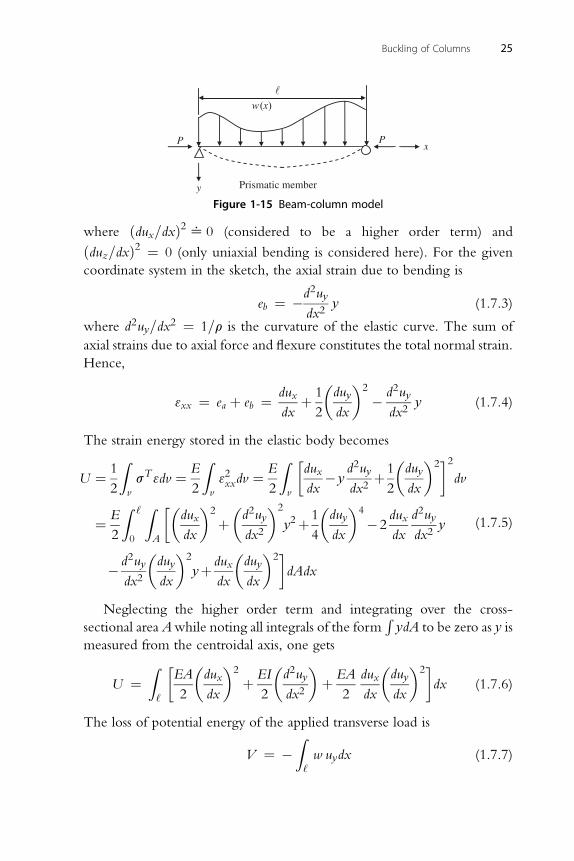
w (x)
Figure 1-15 Beam-column model
Buckling of Columns 25
where ðdux=dxÞ2^ 0 (considered to be a higher order term) and
ðduz=dxÞ2 ¼ 0 (only uniaxial bending is considered here). For the given
coordinate system in the sketch, the axial strain due to bending is
eb ¼ �d2uy
dx2y (1.7.3)
where d2uy=dx2 ¼ 1=r is the curvature of the elastic curve. The sum of
axial strains due to axial force and flexure constitutes the total normal strain.
Hence,
3xx ¼ ea þ eb ¼ dux
dxþ 1
2
�duy
dx
�2
� d2uy
dx2y (1.7.4)
The strain energy stored in the elastic body becomes
¼ 1
2
Zv
sT 3dv ¼ E
2
Zv
32xxdv ¼E
2
Zv
dux
dx� y
d2uy
dx2þ1
2
�duy
dx
�22dv
¼ E
2
Z ‘
0
ZA
�dux
dx
�2
þ�d2uy
dx2
�2
y2þ1
4
�duy
dx
�4
�2dux
dx
d2uy
dx2y
� d2uy
dx2
�duy
dx
�2
yþ dux
dx
�duy
dx
�2dAdx
(1.7.5)
Neglecting the higher order term and integrating over the cross-
sectional area Awhile noting all integrals of the formRydA to be zero as y is
measured from the centroidal axis, one gets
U ¼Z‘
EA
2
�dux
dx
�2
þ EI
2
�d2uy
dx2
�þ EA
2
dux
dx
�duy
dx
�2dx (1.7.6)
The loss of potential energy of the applied transverse load is
V ¼ �Z‘w uydx (1.7.7)

26 Chai Yoo
Hence, the total potential energy functional of the system becomes
P ¼ U þV ¼Z‘
EA
2
�dux
dx
�2
þEI
2
�d2uy
dx2
�þEA
2
dux
dx
�duy
dx
�2
�w uy
dx
(1.7.8)
or
P ¼ U þ V ¼Z‘
EA
2
�dux
dx
�2
þ EI
2
�d2uy
dx2
�� P
2
�duy
dx
�2
� w uy
dx
(1.7.9)
Note that P ¼ sA ¼ EAea ¼ EAðdux=dxÞ, which is called the stress
resultant. The negative sign corresponds to the fact that P is in compression.
The quantity inside the square bracket, the integrand, is denoted by F.
Applying the principle of the minimum potential energy (or applying the
Euler-Lagrange differential equation), one obtains
F ¼ EA
2ðu0Þ2 þ EI
2ðy00Þ2 � P
2ðy0Þ2 � wy (1.7.10)
where u ¼ ux, y ¼ uy .
Recall the Euler-Lagrange DE (see Bleich 1952, pp. 91–103):
Fu � d
dxFu0 þ d2
dx2Fu00 � ::: ¼ 0 (1.7.11)
d d2
Fy �dxFy0 þ
dx2Fy00 � ::: ¼ 0 (1.7.12)
d
Fu ¼ 0; Fu0 ¼ EAu00�dxFu0 ¼ �EAu00; Fu00 ¼ 0;
EAu00 ¼ 0 (1.7.13)
d
Fy ¼ �w; Fy0 ¼ �Py00�dx¼ Py00;
Fy00 ¼ EIy000d2
dx2Fy00 ¼ EIyiv;
EIyiv þ Py00 ¼ w (1.7.14)

Buckling of Columns 27
It should be noted that the concept of finite axial strain implicitly implies the
buckled shape (lateral displacement) and any prebuckling state is ignored.
1.8. GALERKIN METHOD
The requirement that the total potential energy of a hinged column has
a stationary value is shown in the following equation:Z ‘
0
ðEIyiv þ Py00Þdydxþ ðEIy00Þdy0�����‘
0¼ 0 (1.8.1)
where dy is a virtual displacement.
Assume that it is possible to approximate the deflection of the column by
a series of independent functions, gi(x), multiplied by undetermined coef-
ficients, ai.
yapprox ^ a1g1ðxÞ þ a2g2ðxÞ þ ::::::þ angnðxÞ (1.8.2)
If each gi(x) satisfies the geometric and natural boundary conditions, then
the second term in Eq. (1.8.1) vanishes when it substitutes yapprox to y. Also,
the coefficients, ai , must be chosen such that yapproxwill satisfy the first term.
Let the operator be
Q ¼ EId4
dx4þ P
d2
dx2(1.8.3)
and
f ¼Xni¼ 1
aigiðxÞ (1.8.4)
From Eqs. (1.8.3) and (1.8.4), the first term of Eq. (1.8.1.) becomes:Z ‘
0
QðfÞdf dx ¼ 0 (1.8.5)
Since f is a function of n parameters, ai ,
df ¼ vf
va1da1 þ vf
va2da2 þ ::::þ vf
vandan
¼ g1da1 þ g2da2 þ :::::þ gndan ¼Xni¼ 1
gidai
(1.8.6)
Z ‘ Xn
0QðfÞi¼ 1
giðxÞdai dx ¼ 0 (1.8.7)

28 Chai Yoo
Since it has been assumed that gi(x) are independent of each other, the
only way to hold Eq. (1.8.7) is that each integral of Eq. (1.8.7) must vanish,
that is Z ‘
0
QðfÞgiðxÞdai dx ¼ 0 i ¼ 1; 2; :::::; n
ai are arbitrary; hence dai s 0.Z ‘
0
QðfÞgiðxÞdx ¼ 0 i ¼ 1; 2; :::::; n (1.8.8)
Equation (1.8.8) is somewhat similar to the weighted integral process in the
finite element method.
Example 1 Consider the axial buckling of a propped column.
The Galerkin method is to be applied. For yapprox, use the lateral displace-
ment function of a propped beam subjected to a uniformly distributed load.
Hence,
yapprox ¼ f ¼ Aðx‘3 � 3x3‘þ 2x4Þ
d4f d2f
QðfÞ ¼ EIdx4þ P
dx2¼ A½48EI þ Pð24x2 � 18‘xÞ�
3 3 4
gðxÞ ¼ ð‘ x� 3‘x þ 2x ÞZ ‘0
A½48EI þ Pð24x2 � 18‘xÞ�ð‘3x� 3‘x3 þ 2x4Þdx ¼ 0
x
y1
yR
P
0.699
Figure 1-16 Propped column

Buckling of Columns 29
Carrying out the integration gives
A�ð36EI‘5=5Þ � ð12P‘7=35Þ
�¼ 00As0 for a nontrivial solution
Pcr ¼ 21EI=‘2*3:96% greater than the exact value, Pcr exact ¼ 20:2EI=‘2
1.9. CONTINUOUS BEAM-COLUMNS RESTINGON ELASTIC SUPPORTS
A general method to evaluate the minimum required spring constants of
a beam-column resting on an elastic support is to apply the slope-deflection
equations with axial compression. In order to simplify the illustration, all
beam-columns are assumed to be rigid and equal spans.
1.9.1. One SpanAssume that a small displacement occurs at b, so that the bar becomes
inclined to the horizontal by a small angle, a. As the stability of a system is
examined in the neighboring equilibrium position, free body for equilib-
rium must be extracted from a deformed state. Owing to this displacement,
the load P moves to the left by the amount
Lð1� cosaÞ^La2
2(1.9.1)
and the decrease in the potential energy of the load P, equal to the work
done by P, is
PLa2
2(1.9.2)
At the same time the spring deforms by the amount aL , and the increase in
strain energy of the spring is
kðaLÞ22
(1.9.3)
P
LP
k
ba
L
Figure 1-17 One-span model

30 Chai Yoo
where k denotes the spring constant. The system will be stable if
kðaLÞ22
>PLa2
2(1.9.4)
and will be unstable if
kðaLÞ22
<PLa2
2(1.9.5)
Therefore the critical value of the load P is found from the condition
that
kðaLÞ22
¼ PLa2
2(1.9.6)
from which
k ¼ bPcr
L0b ¼ 1 (1.9.7)
The same conclusion can be reached by considering the equilibrium of
the forces acting on the bar. However, if the system has three or more
springs, simple statics may not be sufficient to determine the small
displacement associated with each spring. Hence, the energy method
appears to be better suited.
1.9.2. Two SpanFor small deflection d , the angle of inclination of the bar ab is d/L , and the
distance l moved by the force P is found to be
l ¼ 2
1
2L
�d
L
�2¼ 1
Ld2 (1.9.8)
and the work done by P is
DW ¼ Pl ¼ Pd2
L(1.9.9)
P P
L L
k
a b c
Figure 1-18 Two-span model

Buckling of Columns 31
The strain energy stored in the spring is
DU ¼ kd2
2(1.9.10)
The critical value of the load P is found from the equation
DU ¼ DW (1.9.11)
which represents the condition when the equilibrium configuration
changes from stable to unstable. Hence,
k ¼ bPcr
L¼ 2Pcr
L0b ¼ 2 (1.9.12)
1.9.3. Three SpanFor small displacements, the rotation of bars ab and cd may be
expressed as
a1 ¼ d1
Land a2 ¼ d2
L(1.9.13)
and the rotation of bar bc is
d2 � d1
L(1.9.14)
aR
L L
P P
P1
P2
P1
P2
dba c
k kd
R
1
1
12
2
1 1
– 1
L(a)
(b)
(c)
Figure 1-19 Three-span model

32 Chai Yoo
The distance l moved by the force P is found to be
l ¼ 1
2L
�d1
L
�2
þ�d2 � d1
L
�2
þ�d2
L
�2
¼ 1
2Lðd21 þ d22 þ d21 � 2d1d2 þ d22Þ ¼ 1
Lðd21 � d1d2 þ d22Þ (1.9.15)
and the work done by the force P is
DW ¼ Pl ¼ P
Lðd21 � d1d2 þ d22Þ (1.9.16)
The strain energy stored in the elastic supports during buckling is
DU ¼ k
2ðd21 þ d22Þ (1.9.17)
The critical condition is found by equating these two expressions
P
Lðd21 � d1d2 þ d22Þ ¼ k
2ðd21 þ d22Þ0 P ¼ kL
2
d21 þ d22
d21 � d1d2 þ d22¼ kL
2
N
D
(1.9.18)
where N and D represent the numerator and denominator of the fraction.
To find the critical value of P, one must adjust the deflections d1 and d2,
which are unknown, so as to make P a minimum value. This is accom-
plished by setting vP=vd1 ¼ 0 and vP=vd2 ¼ 0.
vP
vd1¼ kL
2
DðvN=vd1Þ �NðvD=vd1ÞD2
¼ 00
vN
vd1�N
D
vD
vd1¼ vN
vd1� 2P
kL
vD
vd1¼ 0
(1.9.19)
Similarly,vN
vd2� 2P
kL
vD
vd2¼ 0 (1.9.20)
and
vN
vd1¼ 2d1;
vN
vd2¼ 2d2;
vD
vd1¼ 2d1 � d2;
vD
vd2¼ 2d2 � d1 (1.9.21)
Substituting these values, one obtains
2d1 � 2P
kLð2d1 � d2Þ ¼ d1
�1� 2P
kL
�þ d2
P
kL¼ 0 (1.9.22)

2P P�
2P�
2d2 �kL
ð2d2 � d1Þ ¼ d1kL
þ d2 1�kL
¼ 0 (1.9.23)
For nontrivial solutions, the coefficient determinant must vanish.
Hence,
1�2P
kL
P
kL
P
kL1�2P
kL
��������
��������¼ 00
�1�2P
kL
�2
��P
kL
�2
¼ 00P1 ¼ kL
3; P2 ¼ kL
(1.9.24)
The critical load P1 corresponds to the buckling mode shape shown in
Fig. 1-19(b), and the critical load P2 corresponds to the buckling mode
shape shown in Fig. 1-19(c). For a given system, the critical load is the small
one. Hence, P1 is the correct solution. Hence,
k ¼ bPcr
L¼ 3Pcr
L0b ¼ 3 (1.9.25)
The same problem can be solved readily by using equations of equi-
librium. Noting that the reactive force of the spring is given by kd, the end
reactions are
Ra ¼ 2
3kd1 þ 1
3kd2 (1.9.26)
1 2
Buckling of Columns 33
Rd ¼3kd1 þ
3kd2 (1.9.27)
Another equation for Ra is found by taking the moment about point B for
bar ab, which gives
Pd1 ¼ RaL (1.9.28)
and similarly, for ad
Pd2 ¼ RdL (1.9.29)
Combining these four equations yields
P
Ld1 ¼ 2
3kd1 þ 1
3kd20 d1
�2� 3P
kL
�þ d2 ¼ 0 (1.9.30)
P 1 2�
3P�
Ld2 ¼
3kd1 þ
3kd20 d1 þ d2 2�
kL¼ 0 (1.9.31)
34 Chai Yoo
Setting the determinant equal to zero yields”
2� 3P
kL1
1 2� 3P
kL
��������
��������¼
�2� 3P
kL
�2
� 1 ¼ 00P1 ¼ kL
3and P2 ¼ kL
(1.9.32)
By definition, P1 is the correct solution.
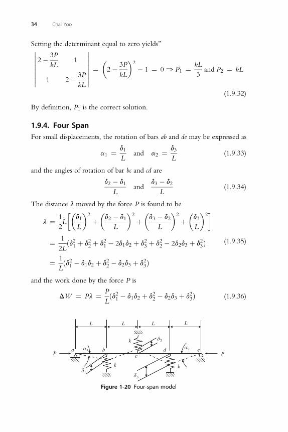
1.9.4. Four SpanFor small displacements, the rotation of bars ab and de may be expressed as
a1 ¼ d1
Land a2 ¼ d3
L(1.9.33)
and the angles of rotation of bar bc and cd are
d2 � d1
Land
d3 � d2
L(1.9.34)
The distance l moved by the force P is found to be
l ¼ 1
2L
�d1
L
�2
þ�d2 � d1
L
�2
þ�d3 � d2
L
�2
þ�d3
L
�2
¼ 1
2Lðd21 þ d22 þ d21 � 2d1d2 þ d23 þ d22 � 2d2d3 þ d23Þ
¼ 1
Lðd21 � d1d2 þ d22 � d2d3 þ d23Þ
(1.9.35)
and the work done by the force P is
DW ¼ Pl ¼ P
Lðd21 � d1d2 þ d22 � d2d3 þ d23Þ (1.9.36)
L
P P
LLL
da bc
e
k
k
k1
2
3
1 2
Figure 1-20 Four-span model

Buckling of Columns 35
The strain energy stored in the elastic supports during buckling is
DU ¼ k
2ðd21 þ d22 þ d23Þ (1.9.37)
The critical condition is found by equating these two expressions
P
Lðd21 � d1d2 þ d22 � d2d3 þ d23Þ ¼ k
2ðd21 þ d22 þ d23Þ0
P ¼ kL
2
d21 þ d22 þ d23
d21 � d1d2 þ d22 � d2d3 þ d23¼ kL
2
N
D
(1.9.38)
where N and D represent the numerator and denominator of the fraction.
To find the critical value of P, one must adjust the deflections d1; d2 and d3,which are unknown, so as to make P a minimum value. This is accom-
plished by setting vP=vd1 ¼ 0; vP=vd2 and vP=vd3 ¼ 0.
vP
vd1¼ kL
2
DðvN=vd1Þ �NðvD=vd1ÞD2
¼ 00
vN
vd1�N
D
vD
vd1¼ vN
vd1� 2P
kL
vD
vd1¼ 0 (1.9.39)
Similarly,
vN
vd2� 2P
kL
vD
vd2¼ 0 (1.9.40)
vN 2P vD
vd3�
kL vd3¼ 0 (1.9.41)
and
vN
vd1¼ 2d1;
vN
vd2¼ 2d2;
vN
vd3¼ 2d3;
vD
vd1¼ 2d1 � d2;
vD
vd2¼ 2d2 � d1 � d3;
vD
vd3¼ 2d3 � d2
(1.9.42)
Substituting these values, one obtains
2d1 � 2P
kLð2d1 � d2Þ ¼ d1
�1� 2P
kL
�þ d2
P
kLþ 0d3 ¼ 0 (1.9.43)

2P P�
2P�
P
2d2 �kLð2d2 � d1 � d3Þ ¼ d1
kLþ d2 1�
kLþ d3
kL¼ 0 (1.9.44)
2P P�
2P�
36 Chai Yoo
2d3 �kL
ð2d3 � d2Þ ¼ 0 d1 þ d2kL
þ d3 1�kL
¼ 0 (1.9.45)
For nontrivial solutions, the coefficient determinant must vanish. Hence,�������������
1� 2P
kL
P
kL0
P
kL1� 2P
kL
P
kL
0P
kL1� 2P
kL
�������������¼
�1� 2P
kL
�3
� 2
�1� 2P
kL
��P
kL
�2
¼�1� 2P
kL
��1� 2P
kL
�2
� 2
�P
kL
�2¼ 0
(1.9.46)
The smallest critical load P1 ¼ 0.29289kL corresponds to the buckling
mode shape shown in sketch.
k ¼ bPcr
L¼ Pcr
0:29289L¼ 3:414Pcr
L0 b ¼ 3:414 (1.9.47)
The equilibrium method cannot be applied to problems with three or
more elastic supports as there are only two equations of equilibrium avail-
able, that is,P
moment ¼ 0 andP
vertical force ¼ 0. It is further noted
that b varies from 1 for one span to 4 for infinite equal spans. Since b equals
3.414 for four equal spans, the use of b ¼ 4 for multistory frames would
seem justified.
Compression members in real structures are not perfectly straight
(sweep, camber), perfectly aligned, or concentrically loaded as is assumed in
design calculations; there is always an initial imperfection. Examining the
single-story column of Fig. 1-17 assuming there is an initial deflection d0reveals that the following equilibrium equation is required:
ðkdÞL ¼ Pðdþ d0Þ (1.9.48)
for P ¼ Pcr
kreqd ¼ Pcr
L
�1þ d0
d
�(1.9.49)

Buckling of Columns 37
Since kideal ¼ Pcr=L, Eq. (1.9.48) becomes
kreqd ¼ kideal
�1þ d0
d
�(1.9.50)
which is the stiffness requirement for compression members having initial
imperfection d0. The stiffness requirement is
Q ¼ kreqdd ¼ kideal
�1þ d0
d
�d ¼ kidealðdþ d0Þ (1.9.51)
Winter (1960) has suggested d ¼ d0 ¼ L/500. Substitution of this into Eqs.
(1.9.49) and (1.9.50) gives the following design equations:
For stiffness; kreqd ¼ 2kideal (1.9.52)
For nominal strength
Qn ¼ kidealð2d0Þ ¼ kidealð0:004LÞ ¼ bPcr
Lð0:004LÞ (1.9.53)
Example 1 Turn-buckled threaded rods (Fy ¼ 50 ksi, Fu ¼ 70 ksi) are
to be provided for the bracing system for a single-story frame shown in
Fig. 1-21. The typical loading on each girder consists of three concentrated
loads. The factored loads are: P1 ¼ 200 kips and P2 ¼ 100 kips. Determine
the diameter of the rod by the AISC (2005) Specification for Structural Steel
Building, 13th edition.
P1 P2P2
20’
20’
20’
15’
25’
Figure 1-21 Single-story frame X-bracing
38 Chai Yoo
XP ¼ 4� ð200þ 2� 100Þ ¼ 1; 600 kips;b ¼ 1;Ae ¼ UAn
¼ 1� An
25
Qu ¼ 1� 1; 600� 0:004 ¼ 6:4 kips; cos q ¼ ffiffiffiffiffiffiffiffiffiffiffiffiffiffiffiffiffiffiffiffiffiffiffið252 þ 152Þp ¼ 0:8575Design for strength
Qn for yielding; Qn ¼ Qu=0:9 ¼ 6:4=0:9 ¼ 7:11 kips
Q for fracture;Q ¼ Q =0:75 ¼ 6:4=0:75 ¼ 8:53 kips
n n uThe required diameter of the rod against yielding is
7:11 ¼ p
4� d2 � 50� 0:8575; d ¼ 0:46 in:
The required diameter of the rod against fracture is
8:53 ¼ p
4��d � 0:9743
11
�2
� 70� 0:8575;
d ¼ 0:154 in:ð11 threads per inch is justifiedÞDesign for stiffness
kreqd ¼ 2kideal ¼ 2bPcr
L¼ 2� 1� 1; 600
25� 12¼ EA
Lcos2 q
2 2
10:67 ¼ 29; 000� p� d � 0:8575
4� 25� 12; d ¼ 0:44 in: < 0:514 in:; use
d ¼ 5=8 in:ð¼ 0:625 in:Þ
1.10. ELASTIC BUCKLING OF COLUMNS SUBJECTED TODISTRIBUTED AXIAL LOADS
When a column is subjected to distributed compressive forces along its
length, the governing differential equation of the deflected curve is no
longer a differential equation with constant coefficients.
The solution to this problem may be considered in three different ways:
(1) application of infinite series such as Bessel functions, (2) one of the
approximate methods, such as the energy method, and (3) the finite element
method (the solution converges to the exact one following the grid

nym
y
x
x
Figure 1-22 Cantilever column subjected to distributed axial load
Buckling of Columns 39
refinement). The energy methods and the finite element analysis will be
illustrated in the next chapter.
Consider the problem of elastic buckling of a prismatic column sub-
jected to its own weight.4,5 Figure 1-22 shows a flagpole-type cantilever
column. The lower end of the column is built in, the upper end is free, and
the weight is uniformly distributed along the column length. Assuming the
buckled shape of the column as shown in Fig. 1-22, the differential equation
of the deflected curve can be shown as:
EId2y
dx2¼
Z ‘
x
qðh� yÞ dx (1.10.1)
where the integral on the right-hand side of the equation represents the
bending moment at any cross section mn produced by the uniformly
distributed load of intensity q. Likewise, the shearing force at any cross
section mn can be expressed as
EId3y
dx3¼ �qð‘� xÞdy
dx(1.10.2)
4 This problem was first discussed by L. Euler (1707–1783), but Euler did not succeed in obtaining
a satisfactory solution according to I. Todhunter, A History of Elasticity and of the Strength of
Materials, edited and completed by K. Pearson, Vol. I (Cambridge: 1886; Dover edition, 1960),
pp. 45–50.5 According to S. Timoshenko and J. Gere, Theory of Elastic Stability (New York: McGraw-Hill,
1961), 2nd ed., pp. 100–103, the problem was solved by A.G. Greenhill (1847–1927) using Bessel
functions.

40 Chai Yoo
Note that the moment given in Eq. (1.10.1) is a decreasing function against
the x-axis, and hence, the rate of change of the moment must be negative as
shown in Eq. (1.10.2). Equation (1.10.2) is an ordinary differential equation
with a variable coefficient. Many differential equations with variable
coefficients can be reduced to Bessel equations. In order to facilitate the
solution, a new independent variable z is introduced such that
z ¼ 2
3
ffiffiffiffiffiffiffiffiffiffiffiffiffiffiffiffiffiffiffiffiffiq
EIð‘� xÞ3
r(1.10.3)
By taking successive derivatives, one obtains
dy
dx¼ dy
dz
dz
dx¼ �dy
dz
ffiffiffiffiffiffiffiffiffi3
2
qz
EI
3
r(1.10.4)
2� �2
3
�2�
d y
dx2¼ 3
2
q
EI
1
3z�
13dy
dzþ z
23d y
dz2(1.10.5)
d3y 3 q�1 dy d2y d3y
�
dx3¼2 EI 9
z�1
dz�dz2
� zdz3
(1.10.6)
Substituting Eqs. (1.10.4) and (1.10.5) into Eq. (1.10.2) and letting
dy
dz¼ u (1.10.7)
One obtains
d2u
dz2þ 1
z
du
dzþ�1� 1
9z2
�u ¼ d2u
dz2þ 1
z
du
dzþ�1� p2
z2
�u ¼ 0 (1.10.8)
Equation (1.10.8) is a Bessel equation, and its solution can be expressed in
terms of Bessel functions.
Invoking the method of Frobenius,6 it is assumed that a solution of the
form
uðzÞ ¼XNn¼ 0
cnzrþn (1.10.9)
exists for Bessel’s equation, Eq. (1.10.8) of 7 order p (�1=3 in this case).
Substituting Eq. (1.10.9) into Eq. (1.10.8), one obtains:
6 Frobenius (1848–1917) was a German mathematician.7 See, for example, S.I. Grossman and W.R. Derrick, Advanced Engineering Mathematics (New York:
Harper & Row, 1988), pp. 272–274.
Buckling of Columns 41
XNn¼ o
cnðr þ nÞðr þ n� 1Þzrþn�2 þXNn¼ o
cnðr þ nÞzrþn�2 þXNn¼ o
ð�p2Þcnzrþn�2
þXNn¼ 2
cn�2zrþn�2 ¼ 0
or
c0ðr2 � p2Þzr�2 þ c1½ðr þ 1Þ2 � p2�zr�1
þXNn¼ 2
fcn½ðnþ rÞ2 � p2� þ cn�2gzrþn�2 ¼ 0(1.10.10)
The indicial equation is r2 � p2 ¼ 0 with roots r1 ¼ p ¼ 1/3 and
r2 ¼ �p ¼ �1/3. Setting r ¼ p in Eq. (1.10.10) yields
ð1þ 2pÞc1zp�1 þXNn¼ 2
½nðnþ 2pÞcn þ cn�2�znþp�2 ¼ 0
�cn�2
indicating that c1 ¼ 0 and cn ¼nðnþ 2pÞ; for n � 2: (1.10.11)
Hence, all the coefficients with odd-numbered subscripts equal to zero.
Letting n ¼ 2j þ 2 one sees that the coefficients with even-numbered
subscripts satisfy
c2ðjþ1Þ ¼ �c2j
22ðj þ 1Þðpþ j þ 1Þ; for j � 0;
which yields
c2 ¼ �c0
22ðpþ 1Þ; c4 ¼ �c2
22ð2Þðpþ 2Þ ¼ c0
24ð2!Þðpþ 1Þðpþ 2Þ;
c6 ¼ �c4
22ð3Þðpþ 3Þ ¼ �c0
26ð3!Þðpþ 1Þðpþ 2Þðpþ 3Þ;.::
Hence, the series of Eq. (1.10.9) becomes
u1 ¼ zpc0 � c0
22ðpþ 1Þz2 þ c0
242!ðpþ 1Þðpþ 2Þz4 � :::
¼ c0zpXNn¼ 0
ð�1Þn z2n
22nn!ðpþ 1Þðpþ 2Þ:::ðpþ nÞ (1.10.12)

42 Chai Yoo
It is customary in Eq. (1.10.12) to let the integral constant,
c0 ¼ ½2pGðpþ 1Þ��1in which Gðpþ 1Þ is the gamma function. Then,
Eq. (1.10.12) becomes
JpðzÞ ¼ ðz=2ÞpXNn¼ 0
ð�1Þn ðz=2Þ2nn!Gðpþ nþ 1Þ
which is known as the Bessel function of the first kind of order p. Thus Jp(z)
is the first solution of Eq. (1.10.8). One will again be able to apply the
method of Frobenius with r ¼ �p to find the second solution. From
Eq. (1.10.10), one immediately obtains
ð1� 2pÞc1z�p�1 þXNn¼ 2
½nðn� 2pÞcn þ cn�2�zn�p�2 ¼ 0 (1.10.13)
indicating c1 ¼ 0 as before and
cn ¼ �cn�2
nðn� 2pÞ (1.10.14)
With algebraic operations similar to those done earlier, one obtains the
second solution of Eq. (1.10.8)
J�pðzÞ ¼ ðz=2Þ�pXNn¼ 0
ð�1Þn ðz=2Þ2nn!Gðn� pþ 1Þ (1.10.15)
Hence, the complete solution of Eq. (1.10.8) is
uðzÞ ¼ u1ðzÞ þ u2ðzÞ ¼ AJpðzÞ þ BJ�pðzÞ (1.10.16)
In Eq. (1.10.16), A and B are constants of integration, and they must be
determined from the boundary conditions of the column. Since the upper
end of the column is free, the condition yields�d2y
dx2
�x¼‘
¼ 0
Observing that z ¼ 0 at x ¼ ‘ and using Eqs. (1.10.5) and (1.10.7), one canexpress this condition as�
1
3z�
13uþ z
23du
dz
�z¼0
¼ 0
Substituting Eq. (1.10.16) into this equation, one obtains A ¼ 0 and
hence
uðzÞ ¼ BJ�pðzÞ (1.10.17)

Buckling of Columns 43
At the lower end of the column the condition is
�dydx
�x¼0
¼ 0
With the use of Eqs. (1.10.3), (1.10.4), and (1.10.7), this condition is
expressed in the form
u ¼ 0 when z ¼ 2
3
ffiffiffiffiffiffiq‘3
EI
r:
The value of z which makes u ¼ 0 can be found from Eq. (1.10.17) by trial
and error, from a table of the Bessel function of order �(1/3) , or from
a computerized symbolic algebraic code such as Maple�. The lowest value
of zwhich makes u¼ 0, corresponding to the lowest buckling load, is found
from Maple� to be z ¼ 1.866350859, and hence
z ¼ 2
3
ffiffiffiffiffiffiq‘3
EI
r¼ 1:866
or
ðqlÞcr ¼ 7:837EI
‘2: (1.10.18)
This is the critical value of the uniform load for the column shown in
Fig. 1-22.
Equation (1.10.2) above is differentiated once more to derive the gov-
erning equation of the buckling of the column under its own weight as
EId2
dx2
�d2y
dx2
�þ q
d
dx
ð‘� xÞdy
dx
¼ 0 (1.10.19)
Equation (1.10.19) is accompanied by appropriate boundary conditions. For
the column that is pinned, clamped, and free at its end, the boundary
conditions are, respectively
y ¼ 0;d2y
dx2¼ 0 (1.10.20a)
dy
y ¼ 0;dx¼ 0 (1.10.20b)
d2y d3y
dx2¼ 0;
dx3¼ 0 (1.10.20c)

44 Chai Yoo
As the differential equation is an ordinary homogeneous equation with
a variable constant, the power series method, or a combination of Bessel and
Lommel functions, are used after a clever transformation. Elishakoff (2005)
gives8 credit to Dinnik (1912) for the solution of the pin-ended column as
ðq‘Þcr ¼ 18:6EI
‘2(1.10.21)
and to Engelhardt (1954) for the solution of the column that is clamped at
one end (bottom) and pinned at the other (top) as
ðq‘Þcr ¼ 52:5EI
‘2(1.10.22)
as well as for the column that is clamped at both ends as
ðq‘Þcr ¼ 74:6EI
‘2(1.10.23)
Structural Stability (STSTB)9 computes critical load for the column that is
clamped at one end (top) and pinned at the other (bottom) as
ðq‘Þcr ¼ 30:0EI
‘2(1.10.24)
Solutions given by Eqs. (1.10.18), (1.10.21), (1.10.22), (1.10.23), and
(1.10.24) can be duplicated closely (within the desired accuracy) by most
present-day computer programs, for example, STSTB. Wang et al. (2005)
present exact solutions for columns with other boundary conditions. A case
of considerable practical importance, in which the moment of inertia of the
column section varies along its length, has been investigated. However,
these problems can be effectively treated by the present-day computer
programs, and efforts associated with the complex mathematical manipu-
lations can now be diverted into other endeavors.
1.11. LARGE DEFLECTION THEORY (THE ELASTICA)
Although it is not likely to be encountered in the construction of buildings
and bridges, a very slender compression member may exhibit a nonlinear
elastic large deformation so that a simplifying assumption of the small
8 I. Elishakoff, Eigenvalues of Inhomogeneous Structures (Boca Raton, FL: CRC Press, 2005), p. 75.9 C.H. Yoo, “Bimoment Contribution to Stability of Thin-Walled Assemblages,” Computers and
Structures, 11, No. 5 (May 1980), pp. 465–471. Fortran source code is available at the senior author’s
Website.

P P
y
x
0θ dx
dyds..sin
dy
dsθ=
Figure 1-23 Large deflection model
Buckling of Columns 45
displacement theory may not be valid, as illustrated by Timoshenko and
Gere (1961) and Chajes (1974). Consider the simply supported wiry
column shown in Fig. 1-23. Aside from the assumption of small deflections,
all the other idealizations made for the Euler column are assumed valid. The
member is assumed perfectly straight initially and loaded along its centroidal
axis, and the material is assumed to obey Hooke’s law.
From an isolated free body of the deformed configuration of the
column, it can be readily observed that the external moment, Py, at any
section is equal to the internal moment, �EI/r.
Thus
Py ¼ �EI
r(1.11.1)
where 1/r is the curvature. Since the curvature is defined by the rate of
change of the unit tangent vector of the curve with respect to the arc length
of the curve, the curvature and slope relationship is established.
1
r¼ dq
ds(1.11.2)
Substituting Eq. (1.11.1) into Eq. (1.11.2) yields
EIdq
dsþ Py ¼ 0 (1.11.3)
Introducing k2 ¼ P/EI, Eq. (1.11.3) transforms into
dq
dsþ k2y ¼ 0 (1.11.4)
Differentiating Eq. (1.11.4) with respect to s and replacing dy/ds by sin q
yields
d2q
ds2þ k2 sin q ¼ 0 (1.11.5)

46 Chai Yoo
Multiplying each term of Eq. (1.11.5) by 2 dq and integrating gives
Zd2qds22dq
dsdsþ
Z2k2 sin q dq ¼ 0 (1.11.6)
Recalling the following mathematical identities
d
ds
�dq
ds
�2
¼ 2
�dq
ds
��d2q
ds2
�and sin q dq ¼ �dðcos qÞ;
it follows immediately thatZd
�dq
ds
�2
� 2k2Z
dðcos qÞ ¼ 0 (1.11.7)
Carrying out the integration gives�dq
ds
�2
� 2k2 cos q ¼ C (1.11.8)
The integral constant C can be determined from the proper boundary
condition. That is
dq
ds¼ 0 at x ¼ 0;�moment ¼ 00
1
r¼ 0 or r ¼ N; straight line
�and q ¼ q0
Hence,
C ¼ �2k2 cos q0
and Eq. (1.11.8) becomes�dq
ds
�2
� 2k2ðcos q� cos q0Þ ¼ 0 (1.11.9)
Taking the square root of Eq. (1.11.9) and rearranging gives
ds ¼ � dqffiffiffi2
pk
ffiffiffiffiffiffiffiffiffiffiffiffiffiffiffiffiffiffiffiffiffiffiffiffiffiffifficos q� cos q0
p (1.11.10)
Notice the negative sign in Eq. (1.11.10), which implies that q decreases as s
increases. Carrying out the integral of Eq. (1.11.10) gives
Buckling of Columns 47
Z ‘=2
0
ds ¼ � 1ffiffiffi2
pk
Z 0
q0
dqffiffiffiffiffiffiffiffiffiffiffiffiffiffiffiffiffiffiffiffiffiffiffiffiffiffifficos q� cos q0
p or‘
2¼ 1ffiffiffi
2p
k
Z q0
0
dqffiffiffiffiffiffiffiffiffiffiffiffiffiffiffiffiffiffiffiffiffiffiffiffiffiffifficos q� cos q0
p
or
‘ ¼ 2
k
Z q0
0
dqffiffiffiffiffiffiffiffiffiffiffiffiffiffiffiffiffiffiffiffiffiffiffiffiffiffiffiffiffiffiffiffiffi2 cos q� 2 cos q0
p (1.11.11)
Notice the negative sign is eliminated by reversing the limits of integration.
Making use of mathematical identities
cos q ¼ 1� 2 sin2q
2and cos q0 ¼ 1� 2 sin2
q0
2
in Eq. (1.11.11) yields:
‘ ¼ 1
k
Z q0
0
dqffiffiffiffiffiffiffiffiffiffiffiffiffiffiffiffiffiffiffiffiffiffiffiffiffiffiffiffiffisin2
q0
2� sin2
q
2
r (1.11.12)
In order to simplify Eq. (1.11.12) further, let
sinq0
2¼ a (1.11.13)
and introduce a new variable f such that
sinq
2¼ a sin f (1.11.14)
Then q ¼ 00f ¼ 0 and q ¼ q00sinf ¼ 10f ¼ p=2.Differentiating Eq. (1.11.14) yields
1
2cos
q
2dq ¼ a cos f df (1.11.15)
which can be rearranged to show
dq ¼ 2a cos f dfffiffiffiffiffiffiffiffiffiffiffiffiffiffiffiffiffiffi1� sin2 q
2
q ¼ 2a cos f dfffiffiffiffiffiffiffiffiffiffiffiffiffiffiffiffiffiffiffiffiffiffiffiffiffi1� a2 sin2 f
p (1.11.16)
Substituting Eqs. (1.11.13), (1.11.14), (1.11.15), and (1.11.16) into Eq.
(1.11.12) yields

48 Chai Yoo
‘ ¼ 1
k
Z q0
0
dqffiffiffiffiffiffiffiffiffiffiffiffiffiffiffiffiffiffiffiffiffiffiffiffiffiffiffiffiffisin2
q0
2� sin2
q
2
r ¼ 1
k
Z p=2
0
1ffiffiffiffiffiffiffiffiffiffiffiffiffiffiffiffiffiffiffiffiffiffiffiffiffiffiffiffia2 � a2 sin2 f
p 2a cosf dfffiffiffiffiffiffiffiffiffiffiffiffiffiffiffiffiffiffiffiffiffiffiffiffiffi1� a2 sin2 f
p
¼ 2
k
Z p=2
0
1
a cosf
a cosf dfffiffiffiffiffiffiffiffiffiffiffiffiffiffiffiffiffiffiffiffiffiffiffiffiffi1� a2 sin2 f
p‘ ¼ 2
k
Z p=2
0
dfffiffiffiffiffiffiffiffiffiffiffiffiffiffiffiffiffiffiffiffiffiffiffiffiffi1� a2 sin2 f
p ¼ 2K
k
(1.11.17)
where:
K ¼Z p=2
0
dfffiffiffiffiffiffiffiffiffiffiffiffiffiffiffiffiffiffiffiffiffiffiffiffiffi1� a2 sin2 f
p (1.11.18)
Equation (1.11.18) is known as the complete elliptic integral of the first kind.
Its value can be readily evaluated from a computerized symbolic algebraic
code such as Maple�. Equation (1.11.17) can be rewritten in the form
‘ ¼ 2K
k¼ 2Kffiffiffiffiffiffiffiffiffiffiffi
P=EIp as k2 ¼ P
EI
or
P
Pcr¼ 4K2
p2(1.11.19)
as
P ¼ 4K2
‘2=EI¼ 4EIK
‘2and Pcr ¼ p2EI
‘2
If the lateral deflection of the member is very small (just after the initial
bulge), then q0 is small and consequently a2 sin2 f in the denominator of K
becomes negligible. The value of K approaches p/2 and from Eq. (1.11.19)
P ¼ Pcr ¼ p2 EI/‘2.The midheight deflection, ym (or d), can be determined from dy¼ ds sin q.
P
PE
Small theory
0
Figure 1-24 Postbuckling behavior

Buckling of Columns 49
Substituting Eq. (1.11.10) into the above equation yields
dy ¼ � sin q dqffiffiffi2
pk
ffiffiffiffiffiffiffiffiffiffiffiffiffiffiffiffiffiffiffiffiffiffiffiffiffiffifficos q� cos q0
p
Integrating the above equation givesZ ym
0
dy ¼ � 1
2k
Z 0
q0
sinqdqffiffiffiffiffiffiffiffiffiffiffiffiffiffiffiffiffiffiffiffiffiffiffiffifficosq� cosq0
p or ym ¼ 1
2k
Z q0
0
sinqdqffiffiffiffiffiffiffiffiffiffiffiffiffiffiffiffiffiffiffiffiffiffiffiffiffiffiffisin2
q0
2� sin2
q
2
r
Recall sin ðq=2Þ ¼ a sinf and dq ¼ 2a cosf df=ffiffiffiffiffiffiffiffiffiffiffiffiffiffiffiffiffiffiffiffiffiffiffiffiffi1� a2 sin2 f
pHence,
sin q ¼ 2 sinq
2cos
q
2¼ 2 sin
q
2
ffiffiffiffiffiffiffiffiffiffiffiffiffiffiffiffiffiffiffi1� sin2
q
2
r¼ 2a sinf
ffiffiffiffiffiffiffiffiffiffiffiffiffiffiffiffiffiffiffiffiffiffiffiffiffi1� a2 sin2 f
pym ¼ 1
2k
Z q0
0
sin q dqffiffiffiffiffiffiffiffiffiffiffiffiffiffiffiffiffiffiffiffiffiffiffiffiffiffiffiffiffisin2
q0
2� sin2
q
2
r
¼ 1
2k
Z p=2
0
2a sinfffiffiffiffiffiffiffiffiffiffiffiffiffiffiffiffiffiffiffiffiffiffiffiffiffiffi1� a2 sin2 f
p2a cosf dfffiffiffiffiffiffiffiffiffiffiffiffiffiffiffiffiffiffiffiffiffiffiffiffiffiffiffiffi
a2 � a2 sin2 fp ffiffiffiffiffiffiffiffiffiffiffiffiffiffiffiffiffiffiffiffiffiffiffiffiffi
1� a2 sin2 fp
Z p=2
ym ¼ d ¼ 2a
k 0
sinf df ¼ 2a
kor
ym‘
¼ 2a
p
ffiffiffiffiffiffiP
PE
rThe distance between the two load points (x-coordinates) can be deter-
mined from
dx ¼ ds cos q
Substituting Eq. (1.11.10) into the above equation yields
dx ¼ � cos q dqffiffiffi2
pk
ffiffiffiffiffiffiffiffiffiffiffiffiffiffiffiffiffiffiffiffiffiffiffiffiffiffifficos q� cos q0
p
Integrating (xm is the x-coordinate at the midheight) the above equation
givesZ xm
0
dx ¼ � 1ffiffiffi2
pk
Z 0
q0
cos q dqffiffiffiffiffiffiffiffiffiffiffiffiffiffiffiffiffiffiffiffiffiffiffiffiffiffifficos q� cos q0
p ¼ � 1ffiffiffik
pZ 0
q0
cos q dqffiffiffiffiffiffiffiffiffiffiffiffiffiffiffiffiffiffiffiffiffiffiffiffiffiffiffiffiffiffiffiffiffi2 cos q� 2 cos q0
p or
xm ¼ 1
2k
Z q0
0
cos q dqffiffiffiffiffiffiffiffiffiffiffiffiffiffiffiffiffiffiffiffiffiffiffiffiffiffiffiffiffisin2
q0
2� sin2
q
2
r

50 Chai Yoo
Recall sin ðq=2Þ ¼ a sinf and dq ¼ 2a cosf df=ffiffiffiffiffiffiffiffiffiffiffiffiffiffiffiffiffiffiffiffiffiffiffiffiffi1� a2 sin2 f
pand cosq ¼ cos2 ðq=2Þ� sin2 ðq=2Þ ¼ 1�2sin2 ðq=2Þ ¼ 1�2a2 sin2f
xm ¼ 1
2k
Z q0
0
cos q dqffiffiffiffiffiffiffiffiffiffiffiffiffiffiffiffiffiffiffiffiffiffiffiffiffiffiffiffiffisin2
q0
2� sin2
q
2
r
¼ 1
2k
Z p=2
0
ð1� 2a2 sin2 fÞ2a cosf dfffiffiffiffiffiffiffiffiffiffiffiffiffiffiffiffiffiffiffiffiffiffiffiffiffiffiffiffia2 � a2 sin2 f
p ffiffiffiffiffiffiffiffiffiffiffiffiffiffiffiffiffiffiffiffiffiffiffiffiffi1� a2 sin2 f
p¼ 1
k
Z p=2
0
ð1� 2a2 sin2 fÞdfffiffiffiffiffiffiffiffiffiffiffiffiffiffiffiffiffiffiffiffiffiffiffiffiffi1� a2 sin2 f
pZ p=2 2 2
x0 ¼ 2xm ¼ 2
k 0
½2ð1� a sin fÞ � 1�dfffiffiffiffiffiffiffiffiffiffiffiffiffiffiffiffiffiffiffiffiffiffiffiffiffi1� a2 sin2 f
p¼ 4
k
Z p=2
0
ffiffiffiffiffiffiffiffiffiffiffiffiffiffiffiffiffiffiffiffiffiffiffiffiffi1� a2 sin2 f
� 2
k
Z p=2
0
dfffiffiffiffiffiffiffiffiffiffiffiffiffiffiffiffiffiffiffiffiffiffiffiffiffi1� a2 sin2 f
p ¼ 4
kEðaÞ � ‘
where E(a) is the complete elliptic integral of the second kind
x0
‘¼ 4EðaÞ
‘
ffiffiffiffiffiP
EI
r � 1 ¼ 4EðaÞp
ffiffiffiffiffiffiP
PE
r � 1
The complete elliptic integral of the first kind can be evaluated by an infinite
series given by
K ¼Z p=2
0
dfffiffiffiffiffiffiffiffiffiffiffiffiffiffiffiffiffiffiffiffiffiffiffiffiffi1� a2 sin2 f
p¼ p
2
1þ
�1
2
�2
a2 þ�1$3
2$4
�2
a4 þ�1$3$5
2$4$6
�2
a6 þ $$$
with a2 < 1
Summing the first four terms of the above infinite series for a ¼ 0:5 yields
K ¼ 1.685174.

Buckling of Columns 51
Likewise, the complete elliptic integral of the second kind can be evaluated
by an infinite series given by
E ¼Z p=2
0
ffiffiffiffiffiffiffiffiffiffiffiffiffiffiffiffiffiffiffiffiffiffiffiffiffi1� a2 sin2 f
¼ p
2
1�
�1
2
�2
a2 ��1$3
2$4
�2a4
3��1$3$5
2$4$6
�2a6
5� $$$
with a2 < 1
Summing the first four terms of the above infinite series for a ¼ 0:5 yields
E ¼1.46746. These two infinite series can be programmed as shown or can
be evaluated by commercially available symbolic algebraic codes such as
Maple�, Matlab�, and/or MathCAD�.

Table 1-1 Load vs. deflection data for large deflection theoryq0 / rad K E a P/PE ym/‘‘ x0/‘‘
0/0 p/2 p/2 .0 1. .0 1.
20/.349 1.583 1.5588 .174 1.015 .110 0.9700
40/.698 1.620 1.5238 .342 1.063 .211 0.8818
60/1.047 1.686 1.4675 .500 1.152 .296 0.7408
90/1.5708 1.8539 1.3507 .707 1.3929 .3814 0.4572
120/2.0944 2.1564 1.2111 .866 1.8846 .4016 0.1233
150/2.618 2.7677 1.0764 .9659 3.1045 .349 �0.2222
170/2.967 4.4956 1.0040 .999 8.1910 .2222 �0.5533
179.996/p 12.55264 1.0000 0.9999999999 63.86 .07966 �0.8407
52 Chai Yoo
Consider the postbuckling shape of the wiry column. This type of
postbuckling behavior may only be imagined for a very thin high-strength
wire. Notice that the two end support positions are reversed. The q0 to
make the two end points contact (x0) is found to be 130.6 degrees by trial
and error. Many ordinary materials may not be able to withstand the
high-stress level required to develop a shape similar to that shown in
Fig. 1-25 in an elastic manner, and the stresses in the critical column
sections are likely to be extended well into the plastic region. Therefore,
the practical value of the large deflection theory at large deflections is
questionable.
Figure 1-25 Postbuckling shape of wiry column
1.12. ECCENTRICALLY LOADED COLUMNSdSECANTFORMULA
In the derivation of the Euler model, a both-end pinned column, it is
assumed that the member is perfectly straight and homogeneous, and that

Buckling of Columns 53
the loading is assumed to be concentric at every cross section so that the
structure and loading are symmetric. These idealizations are made to
simplify the problem. In real life, however, a perfect column that satisfies all
three conditions does not exist. It is, therefore, interesting to study the
behavior of an imperfect column and compare it with the behavior pre-
dicted by the Euler theory. The imperfection of a monolithic slender
column is predominantly affected by the geometry and eccentricity of
loading. As an imperfect column begins to bend as soon as the initial
amount of the incremental load is applied, the behavior of an imperfect
column can be investigated successfully by considering either an initial
imperfection or an eccentricity of loading.
Consider the eccentrically loaded slender column shown in Fig. 1-26.
From equilibrium of the isolated free body of the deformed configuration,
Eq. (1.12.1) becomes obvious
EIy00 þ Pðeþ yÞ ¼ 0 (1.12.1)
or
y00 þ k2y ¼ �k2e with k2 ¼ P=EI (1.12.2)
It should be noted in Eq. (1.12.2) that the system (both-end pinned pris-
matic column of length ‘ with constant EI) eigenvalue remains unchanged
from the Euler critical load as it is evaluated from the homogeneous
differential equation.
The general solution of Eq. (1.12.2) is
y ¼ yh þ yp ¼ A sin kxþ B cos kx� e (1.12.3)
P x
P
P
x
e
y
P
Mx = P(e + y)
Figure 1-26 Eccentrically loaded column

54 Chai Yoo
The integral constants are evaluated from the boundary conditions. (The
notion of solving an nth order ordinary differential equation implies that
a direct or an indirect integral process is applied n times and hence there
should be n integral constants in the solution of an nth order equation.)
Thus the conditiony ¼ 0 at x ¼ 0
leads to
B ¼ e
and the conditiony ¼ 0 at x ¼ ‘
gives
A ¼ e1� cos k‘
sin k‘
Substituting A and B into Eq. (1.12.3) yields
y ¼ e
�cos kxþ 1� cos k‘
sin k‘sin kx� 1
�(1.12.4)
Letting x ¼ ‘/2 in Eq. (1.12.4) for the midheight deflection, d, gives
y
���x¼‘=2
¼ d ¼ e
�cos
k‘
2þ 1� cos k‘
sin k‘sin
k‘
2� 1
�
¼ e
�cos
k‘
2þ1� 1þ 2 sin2
k‘
2
2 sink‘
2cos
k‘
2
sink‘
2� 1
�
d ¼ e
�sec
k‘
2� 1
�¼ e
sec
�p
2
ffiffiffiffiffiffiP
PE
r �� 1
with PE ¼ p2EI
‘2
(1.12.5)
The same deflection curve can be obtained using a fourth-order differential
equation,
y ¼ A cos kxþ B sin kxþ CxþD
with
y ¼ 0; EIy00 ¼ �Pe at x ¼ 0 and
y ¼ 0; EIy00 ¼ �Pe at x ¼ ‘:

0. 2.0 4.0 6.0
0.5
1.0e=0.1
e=0.3
/P PE
Midheight deflection,
Figure 1-27 Load vs. deflection, eccentrically loaded column
Buckling of Columns 55
Figure 1-27 shows the variation of the midheight deflection for two values
of eccentricity, e.
The behavior of an eccentrically loaded column is essentially the same as
that of an initially bent column except there will be the nonzero initial
deflection at the no-load condition in the case of a column initially bent. A
slightly imperfect column begins to bend as soon as the load is applied. The
bending remains small until the load approaches the critical load, after
which the bending increases very rapidly. Hence, the Euler theory provides
a reasonable design criterion for real imperfect columns if the imperfections
are small.
The maximum stress in the extreme fiber is due to the combination of
the axial stress and the bending stress. Hence,
smax ¼ P
AþMmaxc
I¼ P
Aþ Pðdþ eÞc
I¼ P
AþcePsec
�‘
2
ffiffiffiffiffiP
EI
r �I
¼ P
A
1þ ecA
Isec
�‘
2
ffiffiffiffiffiP
EI
r �(1.12.6)
� ffiffiffiffiffiffiffir �
smax ¼ PA1þ ec
r2sec
‘
2r
P
EA(1.12.7)
Equation (1.12.7) is known as the secant formula. In an old edition of
Standard Specification of Highway Bridges, American Association of State

56 Chai Yoo
Highway and Transportation Official (AASHTO) stipulated a constant
value of 0.25 to account for a minimum initial imperfection usually
encountered in practice, as shown in Eq. (1.12.8)
sAASHTO ¼ P
A
1þ
�0:25þ ec
r2
�sec
�‘
2r
ffiffiffiffiffiffiffiP
EA
r �(1.12.8)
1.13. INELASTIC BUCKLING OF STRAIGHT COLUMN
In the discussions presented heretofore, the assumption has been made that
thematerial obeys Hooke’s law. For this assumption to be valid, the stresses in
the column must be below the proportional limit of the material. The linear
elastic analysis is correct for slender columns. On the other hand, the axial
stress in a shot column will exceed the proportional limit. Consequently, the
elastic analysis is not valid for short columns, and the limiting load for short
columns must be determined by taking inelastic behavior into account.
Before proceeding to consider the development of the theory of inelastic
column behavior, it would be informative to review its historic perspective.
The Euler hyperbola was derived by Leonhard Euler in 1744. It was believed
at the time that the formula applied to all columns, short and slender. It was
soon discovered that the formula was grossly unconservative for short
columns; the Euler formula was considered to be completely erroneous and
was discarded for a lengthy period of time, approximately 150 years. An
anecdotal story reveals that people ridiculed Euler when he could not
adequately explain why a coin (a compression member with an extremely
small slenderness ratio) on an anvil smashed by a hammer yielded (flattened)
instead of carrying an infinitely large stress. It is of interest to note that the
concept of flexural rigidity, EI, was not clearly defined at the time, and the
modulus of elasticity of steel was determined by Thomas Young in 1807.10
However, Theodore von Karman developed the double-modulus theory
in 1910 in his doctoral dissertation at Gottingen University under Ludwig
Prandtl direction. It gained widespread acceptance and the validity of Euler’s
work reestablished if the constant modulus E is replaced by an effective
modulus for short columns. Later in 1947, F.R. Shanley11 demonstrated that
the tangent modulus and not the double modulus is the correct effective
modulus, which leads to lower buckling load than the double-modulus
10 S.P. Timoshenko, History of Strength of Materials (New York: Dover Edition, 1983), p. 92.11 A. Chajes, Principles of Structural Stability Theory (Englewood Cliffs, NJ: Prentice-Hall, 1974), p. 37.
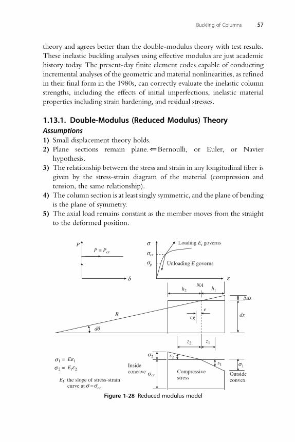
Buckling of Columns 57
theory and agrees better than the double-modulus theory with test results.
These inelastic buckling analyses using effective modulus are just academic
history today. The present-day finite element codes capable of conducting
incremental analyses of the geometric and material nonlinearities, as refined
in their final form in the 1980s, can correctly evaluate the inelastic column
strengths, including the effects of initial imperfections, inelastic material
properties including strain hardening, and residual stresses.
1.13.1. Double-Modulus (Reduced Modulus) TheoryAssumptions1) Small displacement theory holds.
2) Plane sections remain plane.*Bernoulli, or Euler, or Navier
hypothesis.
3) The relationship between the stress and strain in any longitudinal fiber is
given by the stress-strain diagram of the material (compression and
tension, the same relationship).
4) The column section is at least singly symmetric, and the plane of bending
is the plane of symmetry.
5) The axial load remains constant as the member moves from the straight
to the deformed position.
Et: the slope of stress-straincurve at = cr
PP = Pcr
cr
p Unloading E governs
Loading Et governs
Compressivestress
1
2
R
d
e
cg
NAh2 h1
dx
dx
cr
s2
s1
z2 z1
Outsideconvex
Insideconcave
1 = E 1
2 = Et 2
Figure 1-28 Reduced modulus model

58 Chai Yoo
In small displacement theory, the curvature of the bent column is
1
R^
d2y
dx2¼ df
dx(1.13.1)
From a similar triangle relationship, the flexural strains are computed
31 ¼ z1y00 (1.13.2)
3 ¼ z y00 (1.13.3)
2 2and the corresponding stresses are
s1 ¼ Eh1y00 (1.13.4)
s ¼ E h y00 (1.13.5)
2 t 2where Et ¼ tangent modulus, s1 ðtensionÞ ¼ Ez1y00 and s2 ðcompressionÞ ¼
Etz2y00.
The pure bending portion (no net axial force) requires
Z h1
0
s1dAþZ h2
0
s2dA ¼ 0 (1.13.6)
Equating the internal moment to the external moment yields
Z h1
0
s1z1dAþZ h2
0
s2z2dA ¼ Py (1.13.7)
Equation (1.13.6) is expanded to
Ey00Z h1
0
z1dAþ Ety00Z h2
0
z2dA ¼ 0 (1.13.8)
Z h1Z h2
Let Q1 ¼0
z1dA and Q2 ¼0
z2dA0EQ1 þ EtQ2 ¼ 0
(1.13.9)
Equation (1.13.7) is expanded to
y00�E
Z h1
0
z21dAþ Et
Z h2
0
z22dA
�¼ Py (1.13.10)

EI1 þ EtI2
Let E ¼I(1.13.11)
which is called the reduced modulus that depends on the stress-strain
Buckling of Columns 59
relationship of the material and the shape of the cross section. I1 is the
moment of inertia of the tension side cross section about the neutral axis
and I2 is the moment of inertia of the compression side cross section
such that
I1 ¼Z h1
0
z21dA and I2 ¼Z h2
0
z22dA (1.13.12)
Equation (1.13.10) takes the form
EIy00 þ Py ¼ 0 (1.13.13)
Equation (1.13.13) is the differential equation of a column stressed into the
inelastic range identical to Eq. (1.3.3) except that E has been replaced by E,
the reduced modulus. If it can be assumed that E is constant, then Eq.
(1.13.13) is a linear differential equation with constant coefficients, and its
solution is identical to that of Eq. (1.3.3), except that E is replaced by E.
Corresponding critical load and critical stress based on the reduced
modulus are
Pr;cr ¼ p2EI
‘2(1.13.14)
and
sr;cr ¼ p2E�‘
r
�2(1.13.15)
Introducing
sr ¼ E
E¼ Et
E
I2
Iþ I1
I< 1:0 and s ¼ Et
E< 1:0 (1.13.16)
the differential equation based on the reduced modulus becomes
EIsry00 þ Py ¼ 0 (1.13.17)
and
sr ¼ sI2
Iþ I1
Iand sr;cr ¼ Pr;cr
A¼ p2Esr�
‘
r
�2(1.13.18)
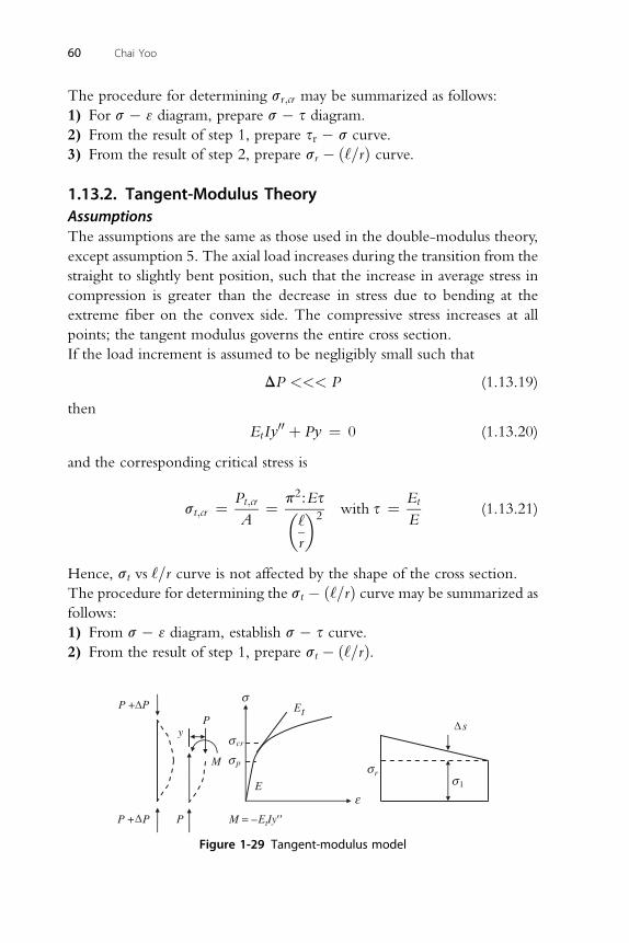
60 Chai Yoo
The procedure for determining sr;cr may be summarized as follows:
1) For s � 3 diagram, prepare s � s diagram.
2) From the result of step 1, prepare sr � s curve.
3) From the result of step 2, prepare sr � ð‘=rÞ curve.
1.13.2. Tangent-Modulus TheoryAssumptionsThe assumptions are the same as those used in the double-modulus theory,
except assumption 5. The axial load increases during the transition from the
straight to slightly bent position, such that the increase in average stress in
compression is greater than the decrease in stress due to bending at the
extreme fiber on the convex side. The compressive stress increases at all
points; the tangent modulus governs the entire cross section.
If the load increment is assumed to be negligibly small such that
DP <<< P (1.13.19)
then
EtIy00 þ Py ¼ 0 (1.13.20)
and the corresponding critical stress is
st;cr ¼ Pt;cr
A¼ p2:Es�
‘
r
�2with s ¼ Et
E(1.13.21)
Hence, st vs ‘=r curve is not affected by the shape of the cross section.
The procedure for determining the st � ð‘=rÞ curve may be summarized as
follows:
1) From s � 3 diagram, establish s � s curve.2) From the result of step 1, prepare st � ð‘=rÞ.
tE
E
y
rp
cr
s
M
P + P
P + P
P
P
M
1
= – EtIy
Figure 1-29 Tangent-modulus model

Buckling of Columns 61
Example 1
An axially loaded, simply supported column is made of structural steel
with the following mechanical properties: E ¼ 30�103 ksi; sp ¼ 28:0ksi;sy ¼ 36ksi; and tangent moduli given in Table 1-2.
Determine the following:
1) The value of ‘/r, which divides the elastic buckling range and the
inelastic buckling range
2) The value of sr and ‘/r for P/A ¼ 28, 30, 32, 34, 35, 35.5 ksi using the
double-modulus theory and assuming that the cross section of the
column is a square of side h.
3) The critical average stress P/A for ‘/r ¼ 20, 40, 60, 80, 100, 120,
140, 160, 180, and 200 using the tangent-modulus theory in the inelastic
range.
From the results of 1), 2), and 3), plot
4) The “ ðP=AÞ � sr” curve for the double-modulus theory.
5) The “ ðP=AÞ � ð‘=rÞ” curves, distinguishing the portion of the curve
derived by the tangent-modulus theory from that derived by the double-
modulus theory. Present short discussions.
6) The current AISC LRFD Specification specifies (Chapter E) that the
critical value of P/A for axially loaded column shall not exceed the
following:
(i) For lc � 1:5 Fcr ¼ ð0:658l2c ÞFy
(ii) For lc > 1:5 Fcr ¼h0:877=l2c
iFy
Plot these curves and superimpose them on the graph in 5 using double
arguments (‘/r and lc) on the horizontal axis.
Table 1-2 Tangent moduli measuredst or sr (ksi) s ¼ Et/E
28.0 1.00
29.0 0.98
30.0 0.96
31.0 0.93
32.0 0.88
33.0 0.77
34.0 0.55
35.0 0.31
35.5 0.16
36.0 0.00

+ z– z
NA
z2 z1
h1h2
h
h
Figure 1-30 Square cross section
62 Chai Yoo
Locations of NA at various stages
EQ1 þ EtQ2 ¼ 0 (1.13.9)
h1 þ h2 ¼ h
Z h1
Q1 ¼0
z1dA
Z h2
Q2 ¼0
z2dA
Z h1�� h 2
Q1 ¼0
z1hdz1 ¼ h
2z21��� 1
0¼ hh1
2
Likewise Q2 ¼ �ðhh22=2Þ
Q1 þ Et
EQ2 ¼
�
hh212
� s
�
hh222
¼ h21 � sðh� h1Þ2 ¼ 0
2 2 2
h1 þ 2shh1 � sh � sh1 ¼ 0ð1� sÞh2 þ 2shh � sh2 ¼ 0
1 1
Table 1-3 Cross-sectional properties vs. shifting neutral axiss
(1)h1(/h)(2)
I1(/I)(3)
I2(/I)(4)
(1) � (4)(5)
sr [(3) þ (5)](6)
s, st, sr
(7)s/s [(7)/(1)](8)
1.00 .5000 .5000 .5000 .5000 1.0000 28.0 28.00
0.98 .4975 .4925 .5076 .4975 0.9899 29.0 29.60
0.96 .4950 .4848 .5155 .4948 0.9797 30.0 31.25
0.93 .4910 .4733 .5277 .4908 0.9640 31.0 33.33
0.88 .4840 .4536 .5495 .4835 0.9371 32.0 36.36
0.77 .4674 .4084 .6044 .4654 0.8738 33.0 42.86
0.55 .4258 .3088 .7572 .4165 0.7253 34.0 61.82
0.31 .3576 .1830 1.0602 .3287 0.5116 35.0 112.90
0.16 .2857 .0933 1.4577 .2332 0.3265 35.5 221.88
0.00 .0000 .0000 4.0000 .0000 0.0000 36.0 N
Buckling of Columns 63
�shþ ffiffiffiffiffiffiffiffiffiffiffiffiffiffiffiffiffiffiffiffiffiffiffiffiffiffiffiffiffiffiffiffiffiffiffiffiffiffiffis2h2 þ ð1� sÞðsh2Þp
hð�sþ ffiffiffis
p Þ
h1 ¼ ð1� sÞ ¼ ð1� sÞp2Es p2 � 30� 103s
sr ¼ r�‘
r
�2¼ r�
‘
r
�20
�‘
r
�¼
ffiffiffiffiffiffiffiffiffiffiffiffiffiffiffiffiffiffiffiffiffiffiffiffiffiffiffi30� 103 p2sr
sr
s¼ 544:14
ffiffiffiffiffisrsr
r
1)
sP ¼ p2E�‘
r
�20
‘
r¼ p
ffiffiffiffiffiE
sp
s¼ 102:83
2) and 3)
Table 1-4 Slenderness ratio vs. critical stress‘‘/r sr ‘‘/r lc Fcr AISC st/s st Remarks
102.83 28.0 200 2.21 6.49 7.402 7.402 gelastic100.53 29.0 180 1.98 8.01 9.138 9.138
98.33 30.0 160 1.76 10.14 11.566 11.566
95.96 31.0 140 1.54 13.25 15.107 15.107
(Continued)

Table 1-4 Slenderness ratio vs. critical stressdcont'd‘‘/r sr ‘‘/r lc Fcr AISC st/s st Remarks
93.12 32.0 120 1.32 18.03 20.562 20.562
88.54 33.0 100 1.10 21.64 29.609 29.000 g st ; from graph79.47 34.0 80 0.88 25.99 46.264 33.200
65.79 35.0 60 0.66 29.97 82.247 34.200
52.18 35.5 40 0.44 33.18 185.055 35.300
0.00 36.0 20 0.22 35.27 740.220 35.990
0 0.00 36.00 N 36.000
64 Chai Yoo
st ¼ p2Es�‘r
�20
st
s¼ p2E�‘
r
�20 in the elastic range;
s ¼ 1:0 ðst ¼ sr ¼ sEÞ
4) and 5)Stress-Tau
28
30
32
34
36
0 0.2 0.4 0.6 0.8 1Tau
Stress
Figure 1-31 Stress vs. tangential-modulus ratio
6) (i) For lc � 1:50Fcr ¼ ð0:658l2c ÞFy (ii) For lc > 1:50Fcr ¼h0:877=l2c
iFy
where lc ¼ ðk‘=rpÞ ffiffiffiffiffiffiffiffiffiffiffiffiðFy=Ep Þ
Compression members (or elements) may be classified into three
different regions depending on their slenderness ratios (or width-to-
thickness ratios): yield zone, inelastic transition zone, and elastic buckling

Stress - Reduced Tau
28
30
32
34
36
0 0.2 0.4 0.6 0.8 1Reduced Tau
Stre
ss
Figure 1-32 Stress vs. reduced modulus ratio
Stress - Stress/Tau
28
30
32
34
36
0 100 200 300Stress/Tau
Stress
Figure 1-33 Stress vs. modular ratio
Buckling of Columns 65
zone (or compact, noncompact, and slender). As can be seen from Fig. 1-34,
the tangent-modulus theory reduces the critical compressive stress only
slightly compared to that by the reduced modulus theory in the inelastic
transition zone. Furthermore, both theories give the inelastic critical stresses
much higher (unconservative) for a solid square cross section considered
herein than those computed from the AISC LRFD formulas that are
considered to be representative (Salmon and Johnson 1996) of many test
data scattered over the world reported by Hall (1981). Experience (Yoo et al.
2001; Choi and Yoo 2005) has shown that the effect of the initial imper-
fections is significant in columns of intermediate slenderness, whereas the
presence of residual stresses reduces the elastic buckling strength. The lowest

Critical Stresses
0
5
10
15
20
25
30
35
40
0 50 100 150 200
Slenderness Ratio
Critic
al S
tre
ss
(k
si)
Reduced
TangentAISC-LRFD
Figure 1-34 Critical stress vs. slenderness ratio
66 Chai Yoo
slenderness columns, which fail by yielding in compression, are hardly
affected by the presence of either the initial imperfections or the residual
stresses. Any nonlinear residual stress distributions in girder shapes having
the residual tensile stress reaching up to the yield stress can readily be
examined by present-day finite element codes.
1.14. METRIC SYSTEM OF UNITS
Dimensions in this book are given in English units. Hard conversion factors
to the metric system are given in Table 1-5. The unit of force in the
International System of units (Systeme International) is the Newton (N).
In European countries and Japan, however, the commonly used unit is
kilogram-force (kgf). Both units are included in the table. Metrication is the
process of converting from the various other systems of units used
throughout the world to the metric or SI (Systeme International) system.
Although the process was begun in France in the 1790s and is currently
converted 95% throughout the world, it is confronting stubborn resistance
in a handful of countries. The main large-scale popular opposition to
metrication appears to be based on tradition, aesthetics, cost, and distaste for
a foreign system. Even in some countries where the international system is
officially adopted, some sectors of the industry. or in a special product line,
old tradition units are still being practiced.

Table 1-5 Conversion FactorsSI to English English to SI
Length
1 mm ¼ 0.03937 in 1 in ¼ 25.4 mm
1 m ¼ 3.281 ft 1 ft ¼ 0.3048 m
1 km ¼ 0.6214 mi 1 mi ¼ 1.609 km
Area
1 mm2 ¼ 1.55 � 10�3 in2 1 in2 ¼ 0.6452 � 103 mm3
1 cm2 ¼ 1.55 � 10�1 in2 1 in2 ¼ 6.452 cm2
1 m2 ¼ 10.76 ft2 1 ft2 ¼ 0.0929 m2
1 m2 ¼ 1.196 yd2 1 yd2 ¼ 0.836 m2
Volume
1 mm3 ¼ 6.102 � 10�5 in3 1 in3 ¼ 16.387 � 103 mm3
1 cm3 ¼ 6.102 � 10�2 in3 1 in3 ¼ 16.387 cm3
1 m3 ¼ 35.3 ft3 1 ft3 ¼ 0.0283 m3
1 m3 ¼ 1.308 yd3 1 yd3 ¼ 0.765 m3
Moment of inertia
1 in4 ¼ 41.62 � 104 mm4 1 mm4 ¼ 0.024 � 10�4 in4
1 in4 ¼ 41.62 cm4 1 cm4 ¼ 0.024 in4
1 in4 ¼ 41.62 � 10�8 m4 1 m4 ¼ 0.024 � 108 in4
Mass
1 kg ¼ 2.205 lb 1 lb ¼ 0.454 kg
1 kg ¼ 1.102 � 10�3 ton 1 ton (2000 lb) ¼ 907 kg
1 Mg ¼ 1.102 ton 1 tonne (metric) ¼ 1000 kg
Force
1 N ¼ 0.2248 lbf 1 lbf ¼ 4.448 N
1 kgf ¼ 2.205 lbf 1 kip ¼ 4.448 kN
Stress
1 kgf/cm2 ¼ 14.22 psi 1 psi ¼ 0.0703 kgf/cm2
1 kN/m2 ¼ 0.145 psi 1 psi ¼ 6.895 kPa (kN/m2)
1 MN/m2 ¼ 0.145 ksi 1 ksi ¼ 6.895 MN/m2 (MPa)
Buckling of Columns 67
GENERAL REFERENCES
Some of the more general references on the stability of structures are
collected in this section for convenience. References cited in the text are
listed at the ends of the respective chapters. References requiring further

68 Chai Yoo
details are given in the footnotes. Relatively recent textbooks and reference
books include those by Bleich (1952), Timoshenko and Gere (1961),
Ziegler (1968), Britvec (1973), Chajes (1974), Brush and Almroth (1975),
Allen and Bulson (1980), Chen and Lui (1991), Bazant and Cedolin (1991),
Godoy (2000), Simitses and Hodges (2006), and Galambos and Surovek
(2008). Some of these books address only the elastic stability of framed
structures, while others extend the coverage into the stability of plates and
shells, including dynamic stability and stability of nonconservative force
systems.
The design of structural elements and components is beyond the scope
of this book. For stability design criteria for columns and plates, Guide to
Stability Design Criteria (Galambos, 1998) is an excellent reference. The
design of highway bridge structures is to be carried out based on AASHTO
(2007) specifications, and steel building frames are to follow AISC (2005)
specifications. In the case of ship structures, separate design rules are stip-
ulated for different vessel types such as IACS (2005) and IACS (2006). A
variety of organizations and authorities are claiming jurisdiction over the
certificates of airworthiness of civil aviation aircrafts.
REFERENCESAASHTO. (2007). LRFD Bridge Design Specifications (4th ed.). Washington, DC: American
Association of State Highway and Transportation Officials.AASHTO. (1973). Standard Specifications for Highway Bridges (11th ed.). Washington, DC:
American Association of State Highway and Transportation Officials.AISC. (2005). Specification for Structural Steel Building (13th ed.). Chicago, IL: American
Institute of Steel Construction.Allen, H. G., & Bulson, P. S. (1980). Background to Buckling. London: McGraw-Hill (UK).Bazant, Z. P., & Cedolin, L. (1991). Stability of Structures, Elastic, Inelastic, Fracture, and
Damage Theories. Oxford: Oxford University Press.Bleich, F. (1952). Buckling Strength of Metal Structures. New York: McGraw-Hill.Britvec, S. J. (1973). The Stability of Elastic Systems. Elmsford, NY: Pergamon Press.Brush, D. O., & Almroth, B. O. (1975). Buckling of Bars, Plates, and Shells. New York:
McGraw-Hill.Chajes, A. (1974). Principles of Structural Stability Theory. Englewood Cliffs, NJ: Prentice-
Hall.Chen, W. F., & Lui, E. M. (1991). Stability Design of Steel Frames. Boca Raton, FL: CRC
Press.Choi, B. H., & Yoo, C. H. (2005). Strength of Stiffened Flanges in Horizontally Curved
Box Girders. J. Engineering Mechanics, ASCE, Vol. 131(No. 2), 167–176, February 2005.Dinnik, A.N. (1912). Buckling Under Own Weight, Proceedings of Don Polytechnic
Institute, 1, Part 2, pp. 12 (in Russian).Elishakoff, I. (2005). Eigenvalues of Inhomogeneous Structures, Unusual Closed-Form Solutions.
Boca Raton, FL: CRC Press.

Buckling of Columns 69
Engelhardt., H. (1954). Die einheitliche Behandlung der Stabknickung mit Berucksichtung desStabeiggengewichte in den Eulerfallen 1 bis 4 als Eigenwertproblem. Der Stahlbau. 23(4),80–84 (in German).
Euler, L. (1744). Methodus Inveniendi Lineas Curvas Maximi Minimive Propreietate Gaudentes(Appendix, De Curvis Elasticis). Lausanne and Geneva: Marcum Michaelem Bousquet.
Galambos, T. V. (Ed.). (1998). Guide to Stability Design Criteria for Metal Structures (5th ed.).New York: Structural Stability Research Council, John Wiley and Sons.
Galambos, T. V., & Surovek, A. E. (2008). Structural Stability of Steel, Concepts and Appli-cations for Structural Engineers. Hoboken, NJ: John Wiley and Sons.
Godoy, L. A. (2000). Theory of Elastic Stability: Analysis and Sensitivity. Philadelphia, PA:Taylor and Francis.
Grossman, S. I., & Derrick, W. R. (1988). Advanced Engineering Mathematics. New York:Harper & Row.
Hall, D. H. (1981). Proposed Steel Column Strength Criteria. J. Structural Div., ASCE,Vol. 107(No. ST4). April 1981, pp. 649–670. Discussed by B.G. Johnston, Vol. 108,No. ST4 (April 1982), pp. 956–957; by Z. Shen and L.W. Lu, Vol. 108, No.ST7(July 1982), pp. 1680–1681; by author, Vol. 108, No. ST12 (December 1982),pp. 2853–2855.
Hoff, N. F. (1956). The Analysis of Structures. New York: John Wiley and Sons.IACS. (2005). Common Structural Rules for Bulk Carriers. London: International Association
of Classification Societies.IACS. (2006). Common Structural Rules for Double Hull Oil Tankers. London: International
Association of Classification Societies.Salmon, C. G., & Johnson, J. E. (1996). Steel Structures, Design and Behavior (4th ed.).
New York: Haper Collins.Salvadori, M., & Heller, R. (1963). Structure in Architecture. Englewood Cliffs, NJ: Prentice-
Hall.Shames, I. H., & Dym, C. L. (1985). Energy and Finite Element Methods in Structural
Mechanics. New York: Hemisphere Publishing Corporation.Simitses, G. J., & Hodges, D. H. (2006). Fundamentals of Structural Stability. Burlington, MA:
Elsevier.Timoshenko, S. P. (1953). History of Strength of Materials. New York: McGraw-Hill.Timoshenko, S. P., & Gere, J. M. (1961). Theory of Elastic Stability (2nd ed.). New York:
McGraw-Hill.Todhunter, I. (1886). In K. Pearson (Ed.) (Dover ed). A History of Elasticity and of the Strength
of Materials, Vol. I. New York: Cambridge. 1960.Wang, C. M., Wang, C. Y., & Reddy, J. N. (2005). Exact Solutions for Buckling of Structural
Members. Boca Raton, FL: CRC Press.Yoo, C. H. (1980). Bimoment Contribution to Stability of Thin-Walled Assemblages.
Computers and Structures, Vol. 11(No. 5), 465–471.Yoo, C. H., Choi, B. H., & Ford, E. M. (2001). Stiffness Requirements for Longitudinally
Stiffened Box Girder Flanges. J. Structural Engineering, ASCE, Vol. 127(No. 6),705–711, June 2001.
Ziegler, H. (1968). Principles of Structural Stability. Waltham, MA: Blaisdell Publishing Co.
PROBLEMS
1.1 For structures shown in Fig. P1-1, determine the following:
(a) Using fourth-order DE, determine the lowest three critical loads.
(b) Determine the lowest two critical loads.
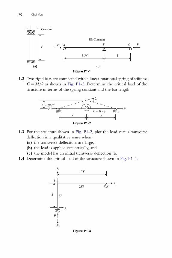
P
A
EI: Constant
B C P
EI: Constant
P
1.5
(a) (b)
Figure P1-1
70 Chai Yoo
1.2 Two rigid bars are connected with a linear rotational spring of stiffness
C ¼M=q as shown in Fig. P1-2. Determine the critical load of the
structure in terms of the spring constant and the bar length.
P PC = M /
= / 2
Figure P1-2
1.3 For the structure shown in Fig. P1-2, plot the load versus transverse
deflection in a qualitative sense when:
(a) the transverse deflections are large,
(b) the load is applied eccentrically, and
(c) the model has an initial transverse deflection d0.
1.4 Determine the critical load of the structure shown in Fig. P1-4.
x1
y1
y2
P
P
2
2EI
EI
x2
Figure P1-4
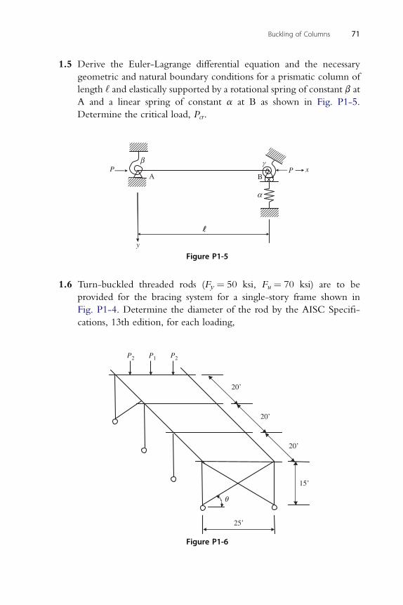
Buckling of Columns 71
1.5 Derive the Euler-Lagrange differential equation and the necessary
geometric and natural boundary conditions for a prismatic column of
length ‘ and elastically supported by a rotational spring of constant b at
A and a linear spring of constant a at B as shown in Fig. P1-5.
Determine the critical load, Pcr.
P
y
A B P x
Figure P1-5
1.6 Turn-buckled threaded rods (Fy ¼ 50 ksi, Fu ¼ 70 ksi) are to be
provided for the bracing system for a single-story frame shown in
Fig. P1-4. Determine the diameter of the rod by the AISC Specifi-
cations, 13th edition, for each loading,
P1 P2P2
20’
20’
20’
15’
25’
Figure P1-6

72 Chai Yoo
(a) when the typical factored loads on each girder are P1 ¼ 250 kips
and P2 ¼ 150 kips, and
(b) when the frame is subjected to a horizontal wind load of intensity
20 psf on the vertical projected area.
1.7 Equation (1.10.22) gives the critical uniformly distributed axial
compressive load as qcr ¼ 52:5EI=ð‘3Þ for a bottom fixed and top
pinned column. Using any appropriate computer program available,
including STSTB, verify that the critical uniformly distributed
compressive load is qcr ¼ 30:0EI=ð‘3Þ for a top fixed and bottom
pinned column.
1.8 An axially loaded, simply supported column is made of structural
steel with the following mechanical properties: E ¼ 30� 103 ksi;sp ¼ 28:0 ksi; sy ¼ 36 ksi; and tangent moduli given in Table 1-2.
h = 2b
b = h / 2
h2
z2
h1
z1
– z + z
N.A.
Figure P1-8 Rectangular cross section
Determine the following:
(a) The value of ‘/r, which divides the elastic buckling range and the
inelastic buckling range.
(b) The value of sr and ‘/r for P/A ¼ 28, 30, 32, 34, 35, 35.5 ksi using the
double-modulus theory and assuming that the cross section of the
column is a rectangle of side b and h ¼ 2b.
(c) The critical average stress P/A for ‘/r ¼ 20, 40, 60, 80, 100, 120, 140,
160, 180, and 200 using the tangent-modulus theory in the inelastic
range.
From the results of a), (b), and (c), plot:

Buckling of Columns 73
(d) The “ ðP=AÞ � sr” curve for the double-modulus theory.
(e) The “ ðP=AÞ � ð‘=rÞ” curves, distinguishing the portion of the curve
derived by the tangent-modulus theory from that derived by the
double-modulus theory. Present short discussions.
(f) The current AISC LRFD Specification specifies (Chapter E) that the
critical value of P/A for axially loaded column shall not exceed the
following:
(i) For lc � 1:5 Fcr ¼ ð0:658l2c ÞFy
(ii) For lc > 1:5 Fcr ¼h0:877=l2c
iFy
Plot these curves and superimpose them on the graph in (e) using
double arguments (‘/r and lc) on the horizontal axis.