Brown Dwarf Companions to Young Solar Analogs: An …
254
Brown Dwarf Companions to Young Solar Analogs: An Adaptive Optics Survey Using Palomar and Keck Thesis by Stanimir A. Metchev In Partial Fulfillment of the Requirements for the Degree of Doctor of Philosophy California Institute of Technology Pasadena, California 2006 (Defended August 18, 2005)
Transcript of Brown Dwarf Companions to Young Solar Analogs: An …

Brown Dwarf Companions to Young Solar Analogs:
An Adaptive Optics Survey Using Palomar and Keck
Thesis byStanimir A. Metchev
In Partial Fulfillment of the Requirementsfor the Degree of
Doctor of Philosophy
California Institute of TechnologyPasadena, California
2006
(Defended August 18, 2005)

ii
c© 2006Stanimir A. MetchevAll Rights Reserved
iii
Acknowledgements
Stan, congratulations. I just can’t believe you made it.Cheers, Jeff Hickey
Having left this for last, I now finally have the peace of mind and hindsight to recollect andthank all the people that supported me, guided me, and kept me sane throughout my graduatework.
First and foremost are my parents, Anguel and Kalitchka, whom I have rarely seen for morethan 2 weeks a year over the past 10 years, but whose faith in me has always pushed me forward,even from the distance of my home country, Bulgaria. I thank my father for showing me thestars and making me aware of a Universe open to endless exploration. I thank my motherfor her unconditional support, even when she thought that I should have taken up Economics,rather than Astronomy. My parents and my brother, Anton, are the three people in this worldthat have defined how I think, feel, and love.
The people that are to blame for my choice of career are the scientists and staff at the NicolaiCopernik National Observatory in my home-town of Varna: Vesselka Radeva, Zahari Donchev,Eva Bojurova, Petar Slavov, Ivan Ivanov, Rudi Kurtev, and the president of amateur astronomyclub “Canopus,” Valentin Velkov. The guiltiest among them are Vesselka and Valentin—theyloaded me with a life-long supply of enthusiasm for astronomy, at the early age of 10.
My graduate advisor, Lynne Hillenbrand, is the person to whom I owe by far the most formy subsequent development as a scientist. I feel very fortunate to have been taken on as herstudent. Lynne’s balance of encouragement and criticism, her ability to manage while allowingindependence, and her camaraderie with her students form a rare ensemble of qualities in anadvisor, with the benefits of which I hope to endebt my own students one day.
For their scientific advice and objectivity (I hope) of judgment, I extend my sincere grat-itude to the past and present members of my thesis committee: Lynne Hillenbrand, AndrewBlain, Shri Kulkarni, Richard Dekany, Re’em Sari, and David Stevenson. I have benefited frommultiple discussions and guidance from every one of them, even before they were confrontedwith the present tome.
I have also been fortunate to be fully immersed in the Formation and Evolution of PlanetarySystems (FEPS) Spitzer Legacy team, which combines a unique array of theoretical and obser-vational expertise on topics ranging from young stars and circumstellar matter to space-basedimaging and high-resolution spectroscopy. Among the members and associates of the teamthat have been most influential on me, I single out Lynne Hillenbrand (again), Michael Meyer,Russel White, Sebastian Wolf, and John Carpenter, with whom I have had the pleasure to workin close collaboration. John also developed and maintains the FEPS team database, that hasbeen of central importance in managing the large volume of data compiled in this thesis.
The quality of the data gathered for this work would have paled in comparison to its presentstate, had it not been for the dedication and professionalism of the Palomar and Keck adaptiveoptics (AO) teams, lead by Mitchell Troy, Richard Dekany, and Peter Wizinowich. Multiplediscussions with Mitch and Rich, as well as with Tom Hayward, Matthew Britton, Hal Petrie,Keith Matthews, David Thompson, Randy Campbell, David Le Mignant, and Marcos vanDam have helped me overcome my initial frustrations with the complexity of AO and become aproficient AO user, excited about the tremendous possibilities offered by the technology. Richand Hal also helped me design the Palomar AO astrometric experiment that proved crucial

iv
for the successful completion of the present work in a timely fashion. Keith provided theastrometric mask for the experiment, as well as key insights for interpreting the experimentdata. Keith and David were also exceptionally kind in obtaining science observations for thepresent work on several occasions.
The Palomar 200-inch telescope was the backbone for my thesis research. With more than70 nights spent at the observatory during my 5 years at Caltech, I am very grateful to the peoplewho made me want to go back there every time: Dipali and Rose for the warm hospitality andthe delicious meals at the Palomar Monastery; Jean Mueller and Karl Dunscombe for theirprofessionalism at the telescope controls and for putting up with my erratic choices of musiclate at night; Rick Burress and Jeff Hickey for their selfless dedication to ensuring the flawlessperformance of the Palomar AO system, and Jeff—for the excellent email greeting on the dayof my defense, quoted at the beginning; Steve, Greg, Dave, John, and the rest of the Palomarday-crew for routinely doing the huge amount of work that it takes every day to keep theobservatory running and the astronomers happy.
With this I come to my close friends. I thank all of you who kept me sane over the yearsand months before my defense, who came to support me during the defense itself, and whocelebrated with me afterwards. In particular, I need to acknowledge my office mates DaveSand, Kevin Bundy, and Josh Eisner. Between them and Russel White, there would always bea good occasion for mid-week drinks at Amigos or at Burger Continental. Also, having gonethrough the job-hunting and thesis ordeals at the same time as Josh and Dave has certainlyhelped me maintain focus and keep the pace.
My close friendship with Alex “Dude” Williamson and the warm hospitality of the Williamsonsand the Redferns has been a staple of my American experience. Alex, Jon, Sue, and DrewWilliamson, and Greg, Laurie, Rachel, and Dan Redfern: thank you all for being my familyaway from home.
Finally, there is one person who saw and heroically put up with the worst of it, and whosedown-to-earth view on life carried me through. My lovely future wife, Anne Simon. I owe youan enormous debt of love and patience. Having you beside me over the past 4 years has givenme a balance that I had never attained before.

v
Abstract
We present results from an adaptive optics survey conducted with the Palomar and Keck tele-scopes over 3 years, which measured the frequency of stellar and sub-stellar companions toSun-like stars. The survey sample contains 266 stars in the 3–10000 million year age range atheliocentric distances between 8 and 200 parsecs and with spectral types between F5–K5. Asub-sample of 101 stars, between 3–500 million years old, were observed in deep exposures witha coronagraph to search for faint sub-stellar companions. A total of 288 candidate companionswere discovered around the sample stars, which were re-imaged at subsequent epochs to deter-mine physical association with the candidate host stars by checking for common proper motion.Benefiting from a highly accurate astrometric calibration of the observations, we were able tosuccessfully apply the common proper motion test in the majority of the cases, including starswith proper motions as small as 20 milli-arcseconds year−1.
The results from the survey include the discovery of three new brown dwarf companions(HD 49197B, HD 203030B, and ScoPMS 214B), 43 new stellar binaries, and a triple system.The physical association of an additional, a priori-suspected, candidate sub-stellar companionto the star HII 1348 is astrometrically confirmed. The newly-discovered and confirmed youngbrown dwarf companions span a range of spectral types between M5 and T0, and will be ofprime significance for constraining evolutionary models of young brown dwarfs and extra-solarplanets.
Based on the 3 new detections of sub-stellar companions in the 101 star sub-sample andfollowing a careful estimate of the survey incompleteness, a Bayesian statistical analysis showsthat the frequency of 0.012–0.072 solar-mass brown dwarfs in 30–1600 AU orbits around youngsolar analogs is 6.8+8.3
−4.9% (2σ limits). While this is a factor of 3 lower than the frequencyof stellar companions to G-dwarfs in the same orbital range, it is significantly higher thanthe frequency of brown dwarfs in 0–3 AU orbits discovered through precision radial velocitysurveys. It is also fully consistent with the observed frequency of 0–3 AU extra-solar planets.Thus, the result demonstrates that the radial-velocity “brown dwarf desert” does not extendto wide separations, contrary to previous belief.

Contents
1 Introduction 11.1 Brown Dwarfs: A Brief Summary of Properties . . . . . . . . . . . . . . . . . . 2
1.1.1 Similarities to Stars . . . . . . . . . . . . . . . . . . . . . . . . . . . . . 21.1.2 Similarities to Planets . . . . . . . . . . . . . . . . . . . . . . . . . . . . 51.1.3 A Matter of Terminology: Low-mass Brown Dwarfs vs. Planets . . . . . 51.1.4 Theoretical Models of Sub-stellar Evolution . . . . . . . . . . . . . . . . 6
1.2 How Frequent are Brown Dwarf Companions and Why Study Them? . . . . . . 71.3 Observational Challenges and Constraints . . . . . . . . . . . . . . . . . . . . . 101.4 The Observational Approach at a Glance . . . . . . . . . . . . . . . . . . . . . 121.5 Thesis Outline . . . . . . . . . . . . . . . . . . . . . . . . . . . . . . . . . . . . 13
2 Survey Sample 142.1 Overview . . . . . . . . . . . . . . . . . . . . . . . . . . . . . . . . . . . . . . . 142.2 Selection Criteria . . . . . . . . . . . . . . . . . . . . . . . . . . . . . . . . . . . 15
2.2.1 Spectral Types and Stellar Masses . . . . . . . . . . . . . . . . . . . . . 152.2.1.1 Spectral Types: Dependence on Color, Reddening, and Surface
Gravity . . . . . . . . . . . . . . . . . . . . . . . . . . . . . . . 152.2.1.2 Masses: Dependence on Age . . . . . . . . . . . . . . . . . . . 17
2.2.2 Stellar Ages . . . . . . . . . . . . . . . . . . . . . . . . . . . . . . . . . . 182.2.3 Distances and Proper Motions . . . . . . . . . . . . . . . . . . . . . . . 23
2.3 Sample Selection . . . . . . . . . . . . . . . . . . . . . . . . . . . . . . . . . . . 242.3.1 FEPS Sample Selection . . . . . . . . . . . . . . . . . . . . . . . . . . . 242.3.2 AO Sample Selection: Further Constraints and Additions . . . . . . . . 25
2.4 Sample Biases and Discussion . . . . . . . . . . . . . . . . . . . . . . . . . . . . 332.4.1 Examining the Biases . . . . . . . . . . . . . . . . . . . . . . . . . . . . . 332.4.2 Discussion . . . . . . . . . . . . . . . . . . . . . . . . . . . . . . . . . . 34
2.5 Unique Advantages of the Present Survey in Comparison to Others . . . . . . . 342.5.1 The Palomar/Keck AO Sample is Young . . . . . . . . . . . . . . . . . . 342.5.2 The Palomar/Keck AO Sample Has a High Median Mass . . . . . . . . . 352.5.3 The Palomar/Keck Survey Uses a High-Order AO System . . . . . . . . 382.5.4 Comparison to Recent, Higher-Contrast Surveys and Summary . . . . . 38
3 Observations and Methodology 393.1 Overview . . . . . . . . . . . . . . . . . . . . . . . . . . . . . . . . . . . . . . . . 393.2 Adaptive Optics Observations of Vega . . . . . . . . . . . . . . . . . . . . . . . 41
3.2.1 Introduction . . . . . . . . . . . . . . . . . . . . . . . . . . . . . . . . . 41
vi
vii
3.2.2 Observations . . . . . . . . . . . . . . . . . . . . . . . . . . . . . . . . . 423.2.3 Data Processing . . . . . . . . . . . . . . . . . . . . . . . . . . . . . . . . 433.2.4 Photometry of Detected Sources . . . . . . . . . . . . . . . . . . . . . . 463.2.5 Analysis . . . . . . . . . . . . . . . . . . . . . . . . . . . . . . . . . . . . 48
3.2.5.1 Sensitivity Limits . . . . . . . . . . . . . . . . . . . . . . . . . 483.2.5.2 Comparisons to Models . . . . . . . . . . . . . . . . . . . . . . 48
3.2.6 Discussion . . . . . . . . . . . . . . . . . . . . . . . . . . . . . . . . . . . 503.2.7 Conclusions . . . . . . . . . . . . . . . . . . . . . . . . . . . . . . . . . . 53
3.3 Initial Results from the PALAO Survey of Young Solar-type Stars . . . . . . . . 543.3.1 Introduction . . . . . . . . . . . . . . . . . . . . . . . . . . . . . . . . . . 543.3.2 Observing Strategy . . . . . . . . . . . . . . . . . . . . . . . . . . . . . 56
3.3.2.1 Imaging . . . . . . . . . . . . . . . . . . . . . . . . . . . . . . . 563.3.2.2 Astrometric Calibration . . . . . . . . . . . . . . . . . . . . . . 603.3.2.3 Spectroscopy . . . . . . . . . . . . . . . . . . . . . . . . . . . . 61
3.3.3 Analysis . . . . . . . . . . . . . . . . . . . . . . . . . . . . . . . . . . . . 633.3.3.1 Photometry . . . . . . . . . . . . . . . . . . . . . . . . . . . . 633.3.3.2 Astrometry . . . . . . . . . . . . . . . . . . . . . . . . . . . . . 663.3.3.3 Spectroscopy . . . . . . . . . . . . . . . . . . . . . . . . . . . . 72
3.3.4 Discussion . . . . . . . . . . . . . . . . . . . . . . . . . . . . . . . . . . . 773.3.4.1 Likelihood of Physical Association . . . . . . . . . . . . . . . . 773.3.4.2 Stellar Ages and Companion Masses . . . . . . . . . . . . . . . 793.3.4.3 HD 129333: Binary or Triple? . . . . . . . . . . . . . . . . . . . 803.3.4.4 HD 49197B: A Rare Young L Dwarf . . . . . . . . . . . . . . . 853.3.4.5 Sub-Stellar Companions to Main-Sequence Stars . . . . . . . . 86
3.3.5 Conclusion . . . . . . . . . . . . . . . . . . . . . . . . . . . . . . . . . . . 88
4 Pixel Scale and Orientation of PHARO 894.1 Pre-amble . . . . . . . . . . . . . . . . . . . . . . . . . . . . . . . . . . . . . . . 894.2 Introduction . . . . . . . . . . . . . . . . . . . . . . . . . . . . . . . . . . . . . 904.3 Experiment Description . . . . . . . . . . . . . . . . . . . . . . . . . . . . . . . 91
4.3.1 Astrometric Mask Experiment . . . . . . . . . . . . . . . . . . . . . . . 914.3.1.1 Assembly . . . . . . . . . . . . . . . . . . . . . . . . . . . . . . 914.3.1.2 Tests . . . . . . . . . . . . . . . . . . . . . . . . . . . . . . . . . 944.3.1.3 Astrometric Measurements . . . . . . . . . . . . . . . . . . . . 96
4.3.2 Binary Stars . . . . . . . . . . . . . . . . . . . . . . . . . . . . . . . . . 984.3.2.1 Observations . . . . . . . . . . . . . . . . . . . . . . . . . . . . 984.3.2.2 Tests . . . . . . . . . . . . . . . . . . . . . . . . . . . . . . . . . 1014.3.2.3 Astrometric Measurements . . . . . . . . . . . . . . . . . . . . 101
4.4 Analysis and Results . . . . . . . . . . . . . . . . . . . . . . . . . . . . . . . . . 1034.4.1 Pixel Scale Distortion as a Function of Detector Position . . . . . . . . . 1034.4.2 Pixel Scale Variation with Hour Angle and Declination . . . . . . . . . . 1044.4.3 Absolute Calibration of the Pixel Scale Distortion . . . . . . . . . . . . 109
4.4.3.1 Additional Parameterization: Beam Tilt . . . . . . . . . . . . . 1094.4.3.2 Solving for the Beam Tilt . . . . . . . . . . . . . . . . . . . . . 1104.4.3.3 Complete Characterization of the Detector Distortion . . . . . . 111
4.4.4 Absolute Pixel Scale of the 25 mas pix−1 PHARO Camera . . . . . . . . 111

viii
4.4.5 Other Sources of Pixel Scale Variations . . . . . . . . . . . . . . . . . . 1154.4.5.1 Cassegrain Ring Orientation . . . . . . . . . . . . . . . . . . . . 1154.4.5.2 Choice of Intermediate Optics . . . . . . . . . . . . . . . . . . . 1164.4.5.3 Detector Readout . . . . . . . . . . . . . . . . . . . . . . . . . 116
4.5 Conclusion of the PHARO Pixel Scale Experiment . . . . . . . . . . . . . . . . . 1164.6 Astrometry with PHARO and NIRC2: Errors and Accuracy . . . . . . . . . . . 117
5 Complete Survey: Observations, Detection, and Association of CandidateCompanions 1195.1 Observations . . . . . . . . . . . . . . . . . . . . . . . . . . . . . . . . . . . . . 119
5.1.1 Choice of PHARO Lyot Stop and the Use of a Neutral Density Filter . . 1305.1.2 Choice of NIRC2 Coronagraphs and Pupil Mask . . . . . . . . . . . . . 1315.1.3 Rotating the Cassegrain Ring at Palomar: The Cons Outweigh the Pros 132
5.2 Object Detection—Limits . . . . . . . . . . . . . . . . . . . . . . . . . . . . . . 1345.2.1 Automatic Source Detection Is Presently Not Well-suited to High-Contrast
AO Imaging . . . . . . . . . . . . . . . . . . . . . . . . . . . . . . . . . . 1345.2.2 Visual Source Detection and Limits . . . . . . . . . . . . . . . . . . . . 1355.2.3 R.M.S. Noise Detection Limits . . . . . . . . . . . . . . . . . . . . . . . 1365.2.4 Ensemble Detection Limits for the Deep Sample . . . . . . . . . . . . . 138
5.3 Detected Candidate Companions . . . . . . . . . . . . . . . . . . . . . . . . . . 1405.4 Deciding Physical Association . . . . . . . . . . . . . . . . . . . . . . . . . . . . 151
5.4.1 Proper Motion . . . . . . . . . . . . . . . . . . . . . . . . . . . . . . . . 1515.4.1.1 Astrometric Example: The Candidate Companions to HD 49197
Re-visited . . . . . . . . . . . . . . . . . . . . . . . . . . . . . 1525.4.2 Absolute Magnitude, Near-IR Colors, and Background Object Density . 1565.4.3 Source Extent . . . . . . . . . . . . . . . . . . . . . . . . . . . . . . . . 1585.4.4 Astrometry from the Literature . . . . . . . . . . . . . . . . . . . . . . . 1595.4.5 Undecided Objects . . . . . . . . . . . . . . . . . . . . . . . . . . . . . . 160
6 Survey Results and Analysis 1616.1 Brown Dwarf Secondaries . . . . . . . . . . . . . . . . . . . . . . . . . . . . . . 161
6.1.1 HD 49197B . . . . . . . . . . . . . . . . . . . . . . . . . . . . . . . . . . 1616.1.2 HD 203030B . . . . . . . . . . . . . . . . . . . . . . . . . . . . . . . . . 165
6.1.2.1 Astrometric Confirmation . . . . . . . . . . . . . . . . . . . . . 1656.1.2.2 Spectral Type and Mass of HD 203030B . . . . . . . . . . . . . 166
6.1.3 ScoPMS 214B . . . . . . . . . . . . . . . . . . . . . . . . . . . . . . . . 1686.1.3.1 Astrometric Confirmation . . . . . . . . . . . . . . . . . . . . . 1686.1.3.2 Spectral Type and Mass of ScoPMS 214B . . . . . . . . . . . . 168
6.1.4 HII 1348B: A Secondary at the Stellar/Sub-stellar Boundary . . . . . . . 1696.1.4.1 Astrometric Confirmation . . . . . . . . . . . . . . . . . . . . . 1696.1.4.2 Spectral Type and Mass of HII 1348B . . . . . . . . . . . . . . 170
6.1.5 A Critical Discussion of Sub-stellar Model Masses: Are the DetectedCompanions Truly Brown Dwarfs? . . . . . . . . . . . . . . . . . . . . . 172
6.2 Incompleteness Analysis of the Deep Survey . . . . . . . . . . . . . . . . . . . . 1736.2.1 Factors Affecting Incompleteness . . . . . . . . . . . . . . . . . . . . . . 1736.2.2 Assumptions . . . . . . . . . . . . . . . . . . . . . . . . . . . . . . . . . 174
ix
6.2.3 Incompleteness Analysis . . . . . . . . . . . . . . . . . . . . . . . . . . . 1756.2.3.1 Geometrical Incompleteness . . . . . . . . . . . . . . . . . . . . 1756.2.3.2 Observational Incompleteness . . . . . . . . . . . . . . . . . . . 1776.2.3.3 Orbital Incompleteness . . . . . . . . . . . . . . . . . . . . . . 1796.2.3.4 Further Incompleteness: Undecided Companion Candidates . . 181
6.3 Frequency of Wide Sub-stellar Companions to Young Solar Analogs . . . . . . . 1826.4 Stellar Secondaries . . . . . . . . . . . . . . . . . . . . . . . . . . . . . . . . . . 184
6.4.1 Frequency of Multiple Systems . . . . . . . . . . . . . . . . . . . . . . . . 1876.4.2 Distribution of Mass Ratios . . . . . . . . . . . . . . . . . . . . . . . . . 1886.4.3 Orbital Motion in Previously Known Binary and Multiple Systems . . . 188
7 Discussion and Summary 1907.1 Comparison to the Results of McCarthy & Zuckerman (2004) . . . . . . . . . . 190
7.1.1 Completeness Estimate of the McCarthy & Zuckerman (2004) Survey . . 1917.1.2 Age Estimate of the McCarthy & Zuckerman (2004) Sample . . . . . . . 192
7.1.2.1 A Space-motion Selected Sample Needs Independent Age Veri-fication . . . . . . . . . . . . . . . . . . . . . . . . . . . . . . . 192
7.1.2.2 The McCarthy & Zuckerman (2004) Sample Is Statistically 1 GyrOld . . . . . . . . . . . . . . . . . . . . . . . . . . . . . . . . . 193
7.1.3 Comparison of Sensitivities to Sub-stellar Companions . . . . . . . . . . 1947.2 Comparison to Previous Multiplicity Results . . . . . . . . . . . . . . . . . . . 194
7.2.1 Other Direct Imaging Surveys for Sub-stellar Companions . . . . . . . . 1947.2.2 Comparison to Planetary and Stellar Multiplicity: No Brown Dwarf
Desert at >30 AU from Solar Analogs . . . . . . . . . . . . . . . . . . . 1967.3 Future Directions . . . . . . . . . . . . . . . . . . . . . . . . . . . . . . . . . . . 1967.4 Summary . . . . . . . . . . . . . . . . . . . . . . . . . . . . . . . . . . . . . . . 198
A Adaptive Optics Imaging of the AU Microscopii Circumstellar Disk: Evi-dence for Dynamical Evolution 199A.1 Introduction . . . . . . . . . . . . . . . . . . . . . . . . . . . . . . . . . . . . . . 200A.2 Observations and Data Reduction . . . . . . . . . . . . . . . . . . . . . . . . . 201A.3 Results and Analysis . . . . . . . . . . . . . . . . . . . . . . . . . . . . . . . . . 204
A.3.1 Circumstellar Dust Morphology . . . . . . . . . . . . . . . . . . . . . . . 204A.3.2 Disk Luminosity, Optical Depth, and Geometry . . . . . . . . . . . . . . 208A.3.3 Detection Limits on Sub-Stellar Companions . . . . . . . . . . . . . . . 208
A.4 Dust Disk Modeling . . . . . . . . . . . . . . . . . . . . . . . . . . . . . . . . . 210A.4.1 Model and Method . . . . . . . . . . . . . . . . . . . . . . . . . . . . . . 210A.4.2 Breaking Degeneracies in the Model Parameters . . . . . . . . . . . . . 211
A.5 Discussion . . . . . . . . . . . . . . . . . . . . . . . . . . . . . . . . . . . . . . . 213A.5.1 Minimum Grain Size as a Function of Disk Radius . . . . . . . . . . . . 215A.5.2 The Change in the SBP Power-law Index: A Comparison with β Pic . . 216
A.5.2.1 Ice or Comet Evaporation . . . . . . . . . . . . . . . . . . . . . 217A.5.2.2 A Belt of Parent Bodies . . . . . . . . . . . . . . . . . . . . . . 217A.5.2.3 Collisional Evolution . . . . . . . . . . . . . . . . . . . . . . . 217A.5.2.4 Poynting-Robertson Drag . . . . . . . . . . . . . . . . . . . . . 218A.5.2.5 Summary of Proposed Scenarios . . . . . . . . . . . . . . . . . . 219

x
A.6 Conclusion . . . . . . . . . . . . . . . . . . . . . . . . . . . . . . . . . . . . . . . 219
List of Figures
1.1 Models of Sub-stellar Luminosity Evolution . . . . . . . . . . . . . . . . . . . . 31.2 Models of Sub-stellar Cooling . . . . . . . . . . . . . . . . . . . . . . . . . . . . 41.3 Color-magnitude Diagram of Brown Dwarfs vs. DUSTY and COND Models . . 8
2.1 Distribution of the Sample Stars as a Function of Teff and M . . . . . . . . . . . 172.2 MKS
vs. J −KS Diagram of the Survey Sample . . . . . . . . . . . . . . . . . . 202.3 Age Distribution of the Survey Sample . . . . . . . . . . . . . . . . . . . . . . . 222.4 Distance and Proper Motion Distributions of the Survey Sample . . . . . . . . . 232.5 Age vs. Distance Diagram of the Survey Sample . . . . . . . . . . . . . . . . . . 36
3.1 Candidate Companions to Vega . . . . . . . . . . . . . . . . . . . . . . . . . . . 453.2 H-band Sensitivity Limits of the Vega Observations . . . . . . . . . . . . . . . . 493.3 Near-IR Color-magnitude Diagrams of the Candidate Companions . . . . . . . . 513.4 Near-IR Color-color Diagram of the Candidate Companions . . . . . . . . . . . 523.5 Images of the Brown Dwarf Companion to HD 49197 . . . . . . . . . . . . . . . 603.6 Images of the Three Stellar Companions . . . . . . . . . . . . . . . . . . . . . . 613.7 K-band Spectra of All Four Companions . . . . . . . . . . . . . . . . . . . . . . 643.8 J-band Spectra of HD 129333B and V522 PerB . . . . . . . . . . . . . . . . . . 653.9 Near-IR Color-color Diagram of the Detected Companions . . . . . . . . . . . . 683.10 Proper Motion Diagram for HD 49197B and “C” . . . . . . . . . . . . . . . . . 703.11 Proper Motion Diagram for HD 129333B . . . . . . . . . . . . . . . . . . . . . . 713.12 Proper Motion Diagrams for V522 PerB and RX J0329.1+0118 . . . . . . . . . 713.13 Comparison of Photometric and Spectroscopically Inferred Absolute Magnitudes 783.14 Radial Velocity Data for HD 129333 . . . . . . . . . . . . . . . . . . . . . . . . . 82
4.1 A Top View of the PALAO Bench . . . . . . . . . . . . . . . . . . . . . . . . . . 924.2 Set-up Diagram for the Astrometric Mask Experiment . . . . . . . . . . . . . . 934.3 A Sketch of the Reticle . . . . . . . . . . . . . . . . . . . . . . . . . . . . . . . . 944.4 A Background-subtracted Image of the Reticle Pattern . . . . . . . . . . . . . . 954.5 Pixel Distances between Neighboring Grid Spots in the Reticle Image . . . . . . 974.6 Images of the Calibration Binary WDS 16147+3352 . . . . . . . . . . . . . . . . 1014.7 Positional and Cassegrain Ring Angle Dependence of the PHARO Pixel Scale . 1024.8 Intrinsic Geometric Distortion of the PHARO Camera in 25 mas pix−1 Mode . . 1054.9 Two-dimensional Polynomial Fits to the Linear Coefficients in Eqns. 4.1 and 4.2 1074.10 Diagram of the Intersection between the Image Plane and the Tilted-beam Plane 1104.11 Positional and Cassegrain Ring Angle Dependence of the PHARO Pixel Scale
after Correcting for Distortion . . . . . . . . . . . . . . . . . . . . . . . . . . . . 1124.12 Total Distortion on the PHARO Camera in 25 mas pix−1 Mode . . . . . . . . . 113
xi
xii
5.1 Example Coronagraphic Images with the Big and Medium Lyot Stops . . . . . . 1315.2 Survey Detection Limits at Palomar and Keck . . . . . . . . . . . . . . . . . . . 1375.3 Contrast and Flux Completeness of the Deep Survey . . . . . . . . . . . . . . . 1395.4 ∆KS vs. Angular Separation for All Candidate Companions . . . . . . . . . . . 1505.5 Proper Motion Diagrams of Candidate Companion 1 to HD 49197 . . . . . . . . 1535.6 Proper Motion Diagrams of Candidate Companion 2 (HD 49197B) to HD 49197 1565.7 MKS
vs. J −KS Color-magnitude Diagram for Candidate Companions with J-band Photometry . . . . . . . . . . . . . . . . . . . . . . . . . . . . . . . . . . . 157
6.1 H–R Diagrams of the New Brown Dwarfs and Model Predictions . . . . . . . . . 1646.2 KS-band Images of HD 203030A/B . . . . . . . . . . . . . . . . . . . . . . . . . 1656.3 Proper Motion Diagrams of HD 203030B . . . . . . . . . . . . . . . . . . . . . . 1666.4 KS-band Images of ScoPMS 214A/B . . . . . . . . . . . . . . . . . . . . . . . . 1696.5 Proper Motion Diagrams of ScoPMS 214B . . . . . . . . . . . . . . . . . . . . . 1706.6 KS-band Images of HII 1348A/B . . . . . . . . . . . . . . . . . . . . . . . . . . 1716.7 Proper Motion Diagrams of HII 1348B . . . . . . . . . . . . . . . . . . . . . . . 1716.8 Projected Physical Separations Probed in the Deep Survey . . . . . . . . . . . . 1766.9 Observational and Orbital Completeness of the Deep Sample Survey . . . . . . . 1786.10 Orbital Incompleteness (SVOC) . . . . . . . . . . . . . . . . . . . . . . . . . . . 1806.11 Probability Density Distribution for the Sub-stellar Companion Frequency in a
Survey of 101 Stars . . . . . . . . . . . . . . . . . . . . . . . . . . . . . . . . . . 1846.12 Distribution of Companion Mass Ratios . . . . . . . . . . . . . . . . . . . . . . . 189
A.1 H-band Images of AU Mic . . . . . . . . . . . . . . . . . . . . . . . . . . . . . . 203A.2 Median Ratios of the Radial Profiles of AU Mic and HD 195720 . . . . . . . . . 204A.3 Reduced Images of the AU Mic Disk . . . . . . . . . . . . . . . . . . . . . . . . 206A.4 H-band Surface Brightness Profiles of the NW and SE Arms of the AU Mic Disk 207A.5 H-band 5σ Detection Limits for Companions to AU Mic . . . . . . . . . . . . . 209A.6 Degeneracies in the Models of the AU Mic SED . . . . . . . . . . . . . . . . . . 212A.7 SED of AU Mic and Disk . . . . . . . . . . . . . . . . . . . . . . . . . . . . . . . 214
List of Tables
2.1 Median Sample Statistics . . . . . . . . . . . . . . . . . . . . . . . . . . . . . . . 152.2 Survey Sample . . . . . . . . . . . . . . . . . . . . . . . . . . . . . . . . . . . . 27
3.1 Near-infrared Point Sources in the Vicinity of Vega . . . . . . . . . . . . . . . . 473.2 Observations . . . . . . . . . . . . . . . . . . . . . . . . . . . . . . . . . . . . . . 573.3 Properties of the Observed Stars . . . . . . . . . . . . . . . . . . . . . . . . . . . 583.4 IR Magnitudes and Colors of the Companions . . . . . . . . . . . . . . . . . . . 673.5 Astrometry of the Companions . . . . . . . . . . . . . . . . . . . . . . . . . . . 693.6 Spectroscopic Measurements for the Companions . . . . . . . . . . . . . . . . . 743.7 Estimated Properties of the Companions . . . . . . . . . . . . . . . . . . . . . . 75
4.1 Observed Calibration Binaries and Parameters of Their Relative Orbits . . . . . 994.2 Observations of Calibration Binaries . . . . . . . . . . . . . . . . . . . . . . . . 1004.3 Preliminary Distortion Coefficients for the 25 mas PHARO Camera with the
Telescope Pointed at Zenith . . . . . . . . . . . . . . . . . . . . . . . . . . . . . 1064.4 Coefficients in the Expansions of a1 (Eqn. 4.3) and b2 (Eqn. 4.4) . . . . . . . . . 1084.5 Final Distortion Coefficients and Expressions at Arbitrary Telescope Hour Angle
and Declination . . . . . . . . . . . . . . . . . . . . . . . . . . . . . . . . . . . . 1084.6 Pixel Scale and Orientation of the 25 mas pix−1 PHARO Camera . . . . . . . . 114
5.1 Palomar Observations . . . . . . . . . . . . . . . . . . . . . . . . . . . . . . . . 1205.2 Keck Observations . . . . . . . . . . . . . . . . . . . . . . . . . . . . . . . . . . 1215.3 Deep Sample Observations . . . . . . . . . . . . . . . . . . . . . . . . . . . . . . 1225.4 Shallow Sample Observations . . . . . . . . . . . . . . . . . . . . . . . . . . . . 1265.5 Magnitude Extinction due to PHARO and NIRC2 Optics . . . . . . . . . . . . . 1315.6 Candidate Companions in the Deep Sample . . . . . . . . . . . . . . . . . . . . 1415.7 Candidate Companions in the Shallow Sample . . . . . . . . . . . . . . . . . . . 1465.8 Deep Sample Stars without Candidate Companions . . . . . . . . . . . . . . . . 1495.9 Shallow Sample Stars without Candidate Companions . . . . . . . . . . . . . . . 1495.10 Observed Change in Relative Position for Candidate Companions to HD 49197 . 1545.11 Expected Change in Relative Position for Candidate Companions to HD 49197 . 1555.12 Color Companions and Their Chance Alignment Probabilities . . . . . . . . . . 159
6.1 Near-IR Photometry of the Confirmed and Candidate Brown Dwarfs . . . . . . 1626.2 Estimated Physical Properties of the Sub-stellar Companions . . . . . . . . . . . 1636.3 Properties of the Detected Stellar Companions . . . . . . . . . . . . . . . . . . . 185
A.1 Preferred Model Parameters for the AU Mic System . . . . . . . . . . . . . . . . 213
xiii

Chapter 1
Introduction
Brown dwarfs make rare companions to stars. This is the current belief in the field of sub-stellarastronomy, based both on precision radial velocity (RV) surveys, probing orbital separationsof <5 astronomical units (AU; Marcy & Butler, 2000), and on direct imaging efforts, prob-ing orbital separations >100 AU (Oppenheimer et al., 2001; McCarthy & Zuckerman, 2004).However, while the radial velocity “brown-dwarf desert” remains nearly void, even after thediscovery of numerous extra-solar planets over the last decade, the direct imaging brown-dwarfdesert appears to be, slowly but surely, becoming populated. How confident are we of thelack of brown dwarfs in wide orbits around stars? Does the direct imaging brown-dwarf desertindeed exist? The few wide brown-dwarf companions that have been imaged around main se-quence stars have provided a disproportionately large wealth of information on the physics ofsub-stellar objects, in comparison with their isolated counterparts. A prime example for thisis Gl 229B–the first decidedly sub-stellar object to be discovered through imaging (Nakajimaet al., 1995) and still the prototype for the coolest objects at the bottom of the main sequence.The reason for this success is the scientifically optimal environment inhabited by brown-dwarfsecondaries in wide orbits. Unlike close-in sub-stellar companions found from RV surveys, wide(> 10−100 AU) brown-dwarf companions are directly accessible for imaging and spectroscopy,thus allowing a characterization of their photospheric and thermodynamic properties. Unlikeisolated free-floating brown dwarfs, brown dwarfs in multiple systems have a well-constrainedage (when physically associated with a star) and may allow a dynamical measurement of theirmass (when in close binaries). That is, wide brown-dwarf companions to stars offer the best op-portunity to fully determine the properties and trace the evolution of sub-stellar objects. Froma scientific point of view, it would be rather unfortunate, if wide brown-dwarf companions tostars did indeed turn out to be rare.
With the present work, we aim to obtain a decisive determination of the frequency of widebrown-dwarf companions to stars. By targeting a large number of young Sun-like stars, weaim to establish a sample of young brown dwarfs with a well-determined age, whose physicalproperties can be used to improve our current knowledge of sub-stellar objects, and that canserve as reference in future studies.
The introductory chapter continues with a brief overview of definitions and brown-dwarfproperties (§1.1). The main scientific goals of the thesis in their justification in the context ofsub-stellar astronomy, are set forth in §1.2. Section §1.3 presents the observational challengesand constraints, and §1.4 summarizes the adopted observational approach for achieving thegoals. Section §1.5 outlines the contents of the thesis by chapters.
1
1.1 Brown Dwarfs: A Brief Summary of Properties 2
1.1 Brown Dwarfs: A Brief Summary of Properties
We start with a brief overview of the physical and observable properties of brown dwarfs, andof their perceived place in our understanding of the Universe in between stars and extra-solarplanets.
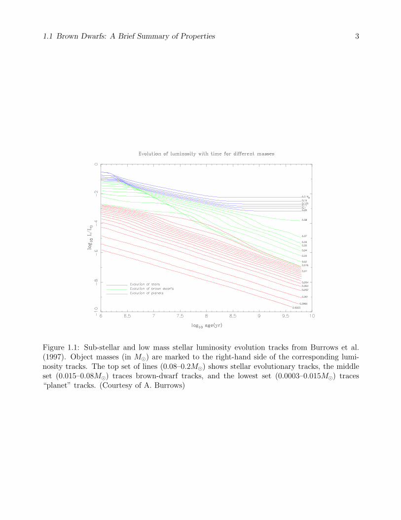
Brown dwarfs are the most recently discovered objects at the bottom of the main sequence.The new spectral types coined for these objects–L and T (Kirkpatrick et al., 1999)–representthe first major extension of the standard Morgan-Keenan OBAFGKM classification scheme(Cannon & Pickering, 1901; Morgan et al., 1943). Implied in this taxonomic expansion is therecognition of the discovery of a fundamentally new type of object. Their masses are too low,less than 0.07–0.08 of a solar mass (M; our Sun is 1M), to ever raise the core temperatureto sufficiently high values (∼ 3 × 10⁶ K) to induce hydrogen fusion (Kumar, 1963; Hayashi& Nakano, 1963; Burrows & Liebert, 1993; Baraffe et al., 1995). Thus, brown dwarfs are“sub-stellar” objects, and, unlike stars, cool eternally. The distinction between stellar and sub-stellar objects is illustrated in Figures 1.1 and 1.2, which show theoretical luminosity evolutiontracks for low-mass stars and brown dwarfs from Burrows et al. (1997, 2001). The bifurcationin the luminosity and effective temperature (Teff) evolution at an age of 0.5–1.0 giga-years(Gyr) straddles the hydrogen-burning mass limit. The exact value of this limit is known tobe metallicity-dependent, ranging from 0.083–0.085M at zero metallicity, to 0.072–0.075Mat solar metallicity (Burrows & Liebert, 1993; Burrows et al., 1997; Chabrier & Baraffe, 1997;Chabrier et al., 2000). Figure 1.1 also demonstrates that, even though massive brown dwarfsmay start out with star-like luminosity (& 10−3 solar luminosities [L]), they progressively dimwith age to the point where all sub-stellar objects are less luminous than the dimmest, lowest-mass, stars after 0.5 Gyr. In terms of effective temperature (Teff) and spectral type, browndwarfs may start as star-like objects hotter than 2200 K, with spectral type M (Kirkpatricket al., 1999). As they get older, brown dwarfs pass through the later L (1400 . Teff . 2200 K;Kirkpatrick et al., 1999; Leggett et al., 2001) and T (Teff . 1300 K; e.g., Burgasser et al., 2002)spectral types (Fig. 1.2).
In sub-stellar interiors luminosity and gas pressure are insufficient to counteract gravity inthe equation of state. Brown dwarfs are thus compact objects, partially supported againstgravitational collapse by electron degeneracy pressure (at early spectral types) and Coulombpressure (at late spectral types; Stevenson, 1991; Burrows & Liebert, 1993). Hence, their radiiR vary only slowly with mass M . The exact functional dependence R(M) is dependent on therelative partition of gas, electron degeneracy, and Coulomb pressure, though for most of thesub-stellar regime varies between R ∝M−1/3 and R ∝M0 (Burrows & Liebert, 1993), i.e., theradii of brown dwarfs are nearly mass-independent.
More detailed, in-depth reviews of the physics of sub-stellar objects can be found in Steven-son (1991); Burrows & Liebert (1993); Chabrier & Baraffe (2000), and Burrows et al. (2001).
1.1.1 Similarities to Stars
Despite their fundamentally different nuclear physics from that of main sequence (MS) stars,brown dwarfs are expected to follow the same mode of formation as (at least low-mass) stars(Bate et al., 2003; Padoan & Nordlund, 2004). That is, there does not exist an a priori setswitch in nature that would distinguish between stellar and sub-stellar objects at the epoch offormation, other than the availability of sufficient accretable mass in the parent environment of
1.1 Brown Dwarfs: A Brief Summary of Properties 3
Figure 1.1: Sub-stellar and low mass stellar luminosity evolution tracks from Burrows et al.(1997). Object masses (in M) are marked to the right-hand side of the corresponding lumi-nosity tracks. The top set of lines (0.08–0.2M) shows stellar evolutionary tracks, the middleset (0.015–0.08M) traces brown-dwarf tracks, and the lowest set (0.0003–0.015M) traces“planet” tracks. (Courtesy of A. Burrows)

1.1 Brown Dwarfs: A Brief Summary of Properties 4
Figure 1.2: Evolution of the effective temperature of low-mass stars and brown dwarfs, aspredicted by Burrows et al. (2001). The sets of continuous lines are the same as in Figure 1.1.Horizontal dashed lines mark the approximate effective temperature limits of the M, L, and Tspectral types. Note that the lowest-mass (≈ 0.08M) hydrogen-burning stars at >3 Gyr agesare L dwarfs, while all >0.010M brown dwarfs start as M dwarfs. The two sets of filled circles(not discussed in the present text) mark the 50% depletion loci for deuterium (left) and lithium(right). (Burrows et al., 2001)

1.1 Brown Dwarfs: A Brief Summary of Properties 5
the objects. Indeed, spectroscopic studies of the initial mass function in 1–5 million-year (Myr)old star-forming regions (Briceno et al., 2002; Luhman et al., 2003b; Slesnick et al., 2004) showno abrupt change in the abundance and spectroscopic signatures between objects above andbelow the hydrogen-burning mass limit. This smooth transition confirms that brown dwarfsare created as a result of a low-mass extension of the star-formation process. Discoveries ofbrown dwarfs have thus shed new light on the range of possible outcomes in environments ofstar formation.
1.1.2 Similarities to Planets
Given the similarity between brown dwarfs and main sequence stars, it may come as a surprisethat brown dwarfs also share common features with planets. Nevertheless, starting with spectraltype T0 and progressing toward later spectral types, the near-IR spectra of brown dwarfs exhibitincreasingly stronger molecular absorption by CH4 and H2 (Burgasser et al., 2002), in additionto the H2O absorption already present in L dwarfs (Kirkpatrick et al., 1999). Conversely,absorption by refractory elements (VO, TiO, and FeH), as characteristic of low-mass M starsin the optical and near-IR (e.g., Leggett et al., 2001), decreases in strength in the L dwarfs,and disappears in the Ts. Thus, at a spectral type of T6.5 (Teff ∼ 900 K; Burgasser et al.,2002), the methane- and water-absorption dominated spectrum of the first discovered browndwarf, Gl 229B (Nakajima et al., 1995; Oppenheimer et al., 1995), resembles the spectra ofsolar-system objects, Jupiter and Titan, more than those of stars. This follows the theoreticalexpectation, that the ultimate state of a cooling brown dwarf, beyond the end of even theexpanded spectral sequence, is a cold, fully degenerate object–much like a planet. Equations ofstate for degenerate interiors also dictate that the radii of L and T dwarfs are similar to thoseof giant gaseous planets, such as Jupiter.
1.1.3 A Matter of Terminology: Low-mass Brown Dwarfs vs. Plan-ets
It is evident from the preceding description (§1.1.1 and §1.1.2) that brown dwarfs occupy anintermediate regime between that of stars and giant planets. High-mass brown dwarfs are likelyto be as indistinguishable from stars at young ages, as low-mass and/or old brown dwarfs arefrom giant planets. Nevertheless, because of the existence of a minimum hydrogen-burningmass, there is a clear separation between brown dwarfs and stars in evolutionary context.Hence, the hydrogen-burning mass limit, albeit not emphasized by an observable transitionbetween the photospheric properties of stars and brown dwarfs at young ages, is defined as theboundary separating the stellar from the sub-stellar regime.
At the low-mass end, the distinction between brown dwarfs and planets is less well-defined.Besides the similarities between their interiors and sizes, the mass regimes of known radial-velocity (RV) extra-solar planets and directly imaged brown dwarfs seem to overlap, in the rangebetween 5 and 15 times the mass of Jupiter (MJup
1). This comes in contrast to the fact thatthe physical processes traditionally perceived as leading to the formation of planets–accretionof planetesimals and gas in a circum-stellar disk (e.g., Lissauer, 1993)–and of more massive,isolated objects (stars and brown dwarfs)–gravo-turbulent fragmentation of a molecular cloud
11MJup = 0.954 × 10⁻³M ≈ 0.001M

1.1 Brown Dwarfs: A Brief Summary of Properties 6
(Bodenheimer et al., 1980; Padoan & Nordlund, 2004)–are very distinct. Recent theories havealso proposed a hybrid process–gravitational instability in a massive circum-stellar disk–for thecreation of both giant planets (Boss, 2002) and brown dwarfs and low-mass stars (Bate et al.,2002). Regardless of the outcome of the theoretical effort to model planet and brown-dwarfformation, the evidence for overlap between the two mass regimes is probably real.
The lack of distinction at the planet/brown-dwarf boundary has spurred some scientific de-bate as to what exactly should be considered a planet and what a brown dwarf. Oppenheimeret al. (2000b) have proposed a distinction analogous to the one established at the stellar/sub-stellar boundary: deciding the classification of an object based on its thermonuclear fusioncapability. Although brown dwarfs do not possess sufficient mass to maintain hydrogen fusion,objects more massive than 0.013–0.015M (depending on metallicity) are expected to undergoa brief deuterium-burning phase (Burrows et al., 1997). The deuterium-burning phase is ex-pressed as a region of slower luminosity and effective temperature decline in > 0.013 M objectsat 3–30 Myr ages in Figures 1.1 and 1.2. Oppenheimer et al. (2000b) choose to define suchdeuterium-burning objects as “brown dwarfs” and reason that lower-mass objects, which neverfuse deuterium, should be referred to as “planets.” Alternative to this is the traditional view ofa planet, upheld by McCaughrean et al. (2001), as an object forming in a circum-stellar disk.The latter definition reserves the term “brown dwarf” for sub-stellar objects formed through astar-like process.
We will generally adhere to the latter terminology, recognizing the fundamental differencebetween the likely modes of formation of planets in our solar system and of brown dwarfsfound in isolation. However, recognizing also the overlap in mass between the latter and knownextrasolar-planets, we will occasionally refer to < 13MJup brown dwarfs as “planetary-massobjects” in the context of their gravitational association with main sequence stars.
1.1.4 Theoretical Models of Sub-stellar Evolution
Because sub-stellar objects never go through a star-like main-sequence phase, their luminositiesand effective temperatures are functions of both mass and age. Observational brown-dwarfscience is thus heavily reliant on theoretical models to accurately predict masses and/or agesfor sub-stellar objects. The present study will not be an exception, though model predictionswill be tested against the limited existing body of empirical data, whenever possible and needed.
Two suites of sub-stellar evolutionary models are used predominantly in the brown-dwarfcommunity, originally due to theoretical teams at the University of Arizona (Burrows et al.,1997)2 and at Ecole Normale Superieure de Lyon (Chabrier et al., 2000; Baraffe et al., 2003).3
The predictions from the two groups are consistent to within 20% in mass at <1Gyr ages. Thepresent investigation will draw on comparisons to both sets of models whenever mass estimatesof specific sub-stellar objects are required. Whenever calculations of solely upper limits areneeded, the Lyon group models will be adopted. Unlike the model from the Arizona group,these tabulate predicted photometry for sub-stellar objects and low-mass stars over a vast rangeof masses (0.0005-0.1 M) and ages (1 Myr–10 Gyr).
The Lyon models come in two flavors: DUSTY (Chabrier et al., 2000) and COND (Baraffeet al., 2003), depending on the treatment of dust opacity in the brown-dwarf photosphere. The
2Publicly available at http://jupiter.as.arizona.edu/˜burrows/3Publicly available at http://perso.ens–lyon.fr/isabelle.baraffe/

1.2 How Frequent are Brown Dwarf Companions and Why Study Them? 7
DUSTY models take into account the formation of dust in the equation of state, and its scatter-ing and absorption in the radiative transfer equation. In this set of models, it is assumed thatdust species remain where they form, according to chemical equilibrium conditions. These mod-els are most appropriate for Teff & 1500 K objects (L dwarfs). For cooler, Teff . 1300 K, objects(T dwarfs), the COND evolutionary tracks model the spectroscopic and photometric propertiesbetter (Baraffe et al., 2003). The COND models are based on the coupling between interiorand non-grey atmosphere structures. The models neglect dust opacity in the radiative transferequation, and applies when all grains have gravitationally settled below the photosphere.
Neither of the two sets of models from the Lyon group account well for the photometricproperties of L-T transitions objects with effective temperatures in the 1300–1500 K range.The proper discussion of this issue requires cloud condensate models (e.g., Ackerman & Marley,2001; Tsuji, 2002; Cooper et al., 2003), none of which have however been tested in evolutionarycontext.
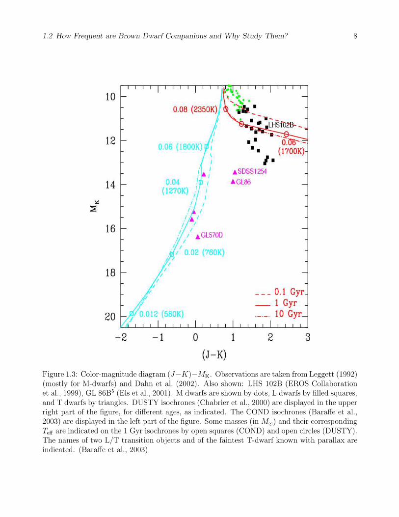
For this temperature range, we will adopt the COND models, which predict absolute near-IR magnitudes that are more consistent with those of late L and early T dwarfs with knowntrigonometric parallaxes (Fig. 1.3)
1.2 How Frequent are Brown Dwarf Companions and
Why Study Them?
Returning to the principle motivation for this work, we re-iterate the presently established viewon the frequency of brown dwarfs around stars. Brown dwarfs make rare companions to stars.The result has been borne out of the prolonged radial velocity (RV) effort to detect sub-stellar(i.e., brown dwarfs and planets) companions to stars, even before RV precision was sufficientlyhigh to allow the detection of extra-solar planets. With more than 150 RV extra-solar planetsnow discovered and less than 10 possible brown dwarfs among them, the dearth of brown-dwarfsecondaries in precision RV surveys remains so dramatic, compared to the relative abundanceof planetary and stellar companions, that the phrase “brown-dwarf desert” is still as pertinentnowadays as when it was originally introduced (Marcy & Butler, 2000). The term provides notonly a vivid representation of the lack of sub-stellar companions of intermediate mass betweenthose of stars and planets, but presumably also of the tremendous scientific and psychologicaltoil of the pioneering RV teams, before perseverance and technological progress laureated theirefforts with success.
Precision RV surveys paint only a partial picture of other stellar systems. They are sensitiveonly to objects with orbital periods of duration comparable to the survey time-span: presently≤ 17 years for the longest-running precision RV surveys, corresponding to orbital semi-majoraxes of ≤5–7 AU from solar-mass stars. At wider orbital separations, corresponding to the gasand ice giant planet zones (5–40 AU) in the solar system, and beyond, little is known. Sub-stellar objects orbiting at >10 AU take too long to complete their orbits to incur a conclusivevelocity trend in present RV surveys.
Our knowledge of sub-stellar multiplicity at such wide separations derives exclusively fromimaging efforts. At small heliocentric distances, wide orbital companions may be sufficientlywell-separated from their host stars to be resolved in direct images of the pair. Contrarily toRV surveys, the greater the orbital separation between the primary star and the secondarycompanion, the easier it is to detect the companion (at a fixed heliocentric distance). For
1.2 How Frequent are Brown Dwarf Companions and Why Study Them? 8
Figure 1.3: Color-magnitude diagram (J−K)−MK. Observations are taken from Leggett (1992)(mostly for M-dwarfs) and Dahn et al. (2002). Also shown: LHS 102B (EROS Collaborationet al., 1999), GL 86B5 (Els et al., 2001). M dwarfs are shown by dots, L dwarfs by filled squares,and T dwarfs by triangles. DUSTY isochrones (Chabrier et al., 2000) are displayed in the upperright part of the figure, for different ages, as indicated. The COND isochrones (Baraffe et al.,2003) are displayed in the left part of the figure. Some masses (in M) and their correspondingTeff are indicated on the 1 Gyr isochrones by open squares (COND) and open circles (DUSTY).The names of two L/T transition objects and of the faintest T-dwarf known with parallax areindicated. (Baraffe et al., 2003)
1.2 How Frequent are Brown Dwarf Companions and Why Study Them? 9
example, given ability to do high-contrast imaging science at ≥0.5′′, the entire giant planetregion outwards of 5 AU can be imaged around a nearby star at 10 pc. In this manner,precision RV and direct imaging surveys explore two complementary orbital realms for sub-stellar companions to nearby stars. However, unlike RV monitoring, which can reveal sub-stellarcompanions a fraction of a Jupiter in mass, direct imaging searches for sub-stellar secondariesto stars are still constrained to companions of multiple Jupiter masses or larger: mainly browndwarfs. Any sub-stellar companions imaged around other stars will therefore be more massivethan any of the known solar system planets. 6
While the pace of RV discoveries has increased steadily since the detection of the first extra-solar planet (Mayor & Queloz, 1995), despite concentrated efforts from a number of teams, therate of brown-dwarf companions discovered via direct imaging has been steadily slow for mostof the same period, despite concentrated efforts from several groups. Two large direct imagingsurveys for sub-stellar companions (Oppenheimer et al., 2001; McCarthy, 2001) have producedonly one brown dwarf (Gl 229B: the first one to be discovered; Nakajima et al., 1995) in acombined sample of over 340 stars and a combined separation range of 10–1200 AU. This resultis in stark contrast both with the frequency of RV extra-solar planets within 3 AU (5–15%;Marcy & Butler, 2000; Fischer et al., 2002) and with the frequency of stellar companions tostars over 10–1200 AU (9–13% for M–G-dwarf primaries; Fischer & Marcy, 1992; Duquennoy &Mayor, 1991). Analogous reasoning has prompted McCarthy & Zuckerman (2004) to concludethat the brown-dwarf desert extends much beyond the 0–5 AU probed by RV surveys. Morerecent results from other, smaller efforts, have been mixed, with surveys performed with moresensitive instrumentation generally reporting higher, though statistically not inconsistent, ratesof success (e.g., 1 out of 50).
This situation is reminiscent of the initial search for sub-stellar companions through the RVmethod, both in the amount of effort invested world-wide and in the, perhaps frustratingly, lowyield. However, the sensitivity of precision RV surveys has much surpassed the brown-dwarfmass regime, whereas imaging efforts are still mostly limited to intermediate- to high-massbrown dwarfs. The RV brown-dwarf desert has remained nearly void even after the discoveryof lower-mass extra-solar planets. Will this be the case with the direct imaging brown-dwarfdesert?
The problem is most comprehensively addressed in the context of Sun-like stars, because ofthe large body of empirical data that exist on the stellar and sub-stellar multiplicity of solaranalogs. The exhaustive study of stellar companions in 0−1010-day periods (0−105 AU) aroundG-dwarfs by Duquennoy & Mayor (1991) finds that the peak of the stellar companion perioddistribution occurs near 105 days (∼35 AU). Duquennoy & Mayor also find that the distributionof the mass ratios q ≡ M1/M2 in binary systems is nearly flat over 0.0 < q ≤ 0.4–a result thathas been confirmed in more recent studies (e.g., Mazeh et al., 2003). Although the results forthe q ≤ 0.1 bin in these studies are largely (Mazeh et al., 2003) or entirely (Duquennoy &Mayor, 1991) extrapolated, beacuse of the severe incompleteness to low-mass companions, itappears plausible that more sensitive studies will detect significant numbers of such secondaries.
6Another technique for detecting sub-stellar companions to stars is by astrometric, rather than spectroscopic(as in the RV approach), measurement of the stellar reflex motion. Similarly to the direct imaging approach,the astrometric technique is more sensitive to companions in wider orbits. Because, like the RV method, theastrometric technique also relies on the detection of orbital motion, it requires longer monitoring periods toprobe the wider orbital separations. As a result, no extra-solar planets have been discovered from astrometricmonitoring yet, though the first brown-dwarf companion was announced recently in Pravdo et al. (2005).
1.3 Observational Challenges and Constraints 10
From the standpoint of precision RV surveys, the frequency of extra-solar planets is rising withorbital separation out to the present completeness limit of the surveys (Marcy et al., 2003;Udry et al., 2003). In addition, the last three years have seen the announcement of severalRV “super-planets,” objects with minimum masses in the 10–25 MJup range, i.e., likely browndwarfs (Udry et al., 2002; Jones et al., 2002; Fischer et al., 2002; Endl et al., 2004). Most ofthese are at semi-major axes wider than 1.5 AU, suggestive of a positive correlation betweenmass and period for RV planets (Zucker & Mazeh, 2002; Udry et al., 2003). That is, even moremassive sub-stellar objects may exist at wider orbital separations from Sun-like stars.
Connecting the above two lines of evidence, there is an indication that brown dwarfs, giventheir intermediate mass between those of stars and extra-solar planets, should exist with someappreciable frequency in wide orbits around Sun-like stars. What fraction of Sun-like stars havesuch widely-separated brown-dwarf secondaries?
This is the principle question guiding the present investigation. By undertaking a largedirect imaging study of a carefully-selected sample of solar analogs, and by employing themodern high-contrast imaging capabilities at the Palomar 5 m and Keck 10 m telescopes, weare able to resolve the issue at a sufficient level of confidence.
Direct imaging investigations of sub-stellar multiplicity are also relevant to the study ofthe photospheric evolution of sub-stellar objects: both brown dwarfs and giant planets. Asmentioned in §1.1, sub-stellar objects never go through a star-like main-sequence phase, dur-ing which their luminosity and effective temperature are largely independent of age and aredetermined mostly by mass. Instead, their luminosity and effective temperature are stronglyage-dependent. With the ages of field brown dwarfs still practically indeterminable, theoreticalbrown-dwarf cooling models have had few empirical constraints beyond the late-M to early-Lbrown dwarfs found in young open clusters. Of strong interest, for example, is more accurateunderstanding of the transition between late L and early T dwarfs: a phenomenon occurring atapproximately constant temperature (∼1300–1500 K; Ackerman & Marley, 2001; Tsuji, 2002)but during which the near-IR J−KS color of a brown dwarf changes by more than a magnitude(Kirkpatrick et al., 1999; Burgasser et al., 2002). No brown dwarfs later than L7 have beenage-dated yet, as none have been confirmed in open clusters or as companions to stars of knownage. The discovery of such late-type brown dwarfs as companions to stars with known ages canprovide much-needed empirical calibration and theoretical constraints. This is a second issuethat will be addressed as a result of the present survey in the near future. At an age of 400 Myrand a photometrically-estimated spectral type of T0, one of the newly-discovered brown-dwarfcompanions is likely the first known young L/T transition object.
Going beyond the concrete goal to test the existence of the brown-dwarf desert at wideseparations, imaging studies of the multiplicity fraction and separation distribution of low massratio (q < 0.1) binaries provide important clues for the mechanism of their formation anddynamical stability (e.g., Close et al., 2003). By virtue of being optimized for the detection ofsub-stellar companions, the present survey provides ample material for future investigations oflow mass ratio systems.
1.3 Observational Challenges and Constraints
The main challenge in direct imaging of sub-stellar companions to stars is achieving sufficientcontrast to detect a faint companion in the vicinity of its orders of magnitude brighter host

1.3 Observational Challenges and Constraints 11
star. Three main factors, addressed in turn below, contribute to this problem: imaging contrastcapability, heliocentric distance to the star, and stellar youth.
Seeing-limited observations through the Earth’s turbulent atmosphere suffer from the largeextent (1′′) of the imaging point-spread function (PSF). The contrast achieved in seeing-limitedimaging is too poor to detect almost any sub-stellar companions within ∼ 10′′ from solaranalogs, i.e., within 100 AU from a star at 10 pc. This problem has been aleviated overthe past decade by the availability of space-based imaging with the Hubble Space Telescope(HST) and of ground-based adaptive optics (AO)–a technique that compensates for atmosphericturbulence through the use of high operational frequency corrective optics. Large AO-equippedtelescopes nowadays routinely produce diffraction-limited PSFs, of order 0.05–0.10′′ on 5–10 mclass telescopes in the near-IR. Such angular resolution rivals that obtained by the HST andallows unprecedented scrutiny of small angular scales. The contrast achieved by various AOsystems and the HST is generally 103−105 at 1′′ from bright stars in the near-IR (1–2.5 µm)–farsuperior than the contrast of seeing-limited observations at the same angular separation (orderunity). However, AO is strongly limited by the need of the corrective system for a sufficientlybright nearby (. 60′′) beacon, a “guide star,” above the turbulent layers in the atmosphereto probe the distortion of the incident radiation. Without the use of an artificial guide star(a laser beam), the celestial distribution of natural guide stars (NGSs) of sufficient apparentbrightness allows the use of AO for only .1% of the total area of the sky. Fortunately, solaranalogs within ∼200 pc are generally sufficiently bright to be used as guide stars themselves,thus allowing full use of the power of NGS AO for the present study.
The apparent angular scale of a stellar system is inversely proportional to its heliocentricdistance: systems that are farther away are more challenging to resolve. Given an interest inimaging orbital separations of solar-system scales around other stars, we are limited in choiceto relatively nearby stars, within 400 pc (40 AU at 0.1′′ resolution). Furthermore, because ofthe inverse-squared dependence of flux on heliocentric distance, sub-stellar objects in farawaysystems may be too faint to detect. In contrast-limited imaging, however, this factor is of lesserimportance.
The contrast attained with AO or the HST may still be inadequate to detect any but themost massive sub-stellar companions in intrinsic light, and is ∼3–5 orders of magnitudes toopoor to detect companions in reflected light. As the detection of intrinsic light offers a clearadvantage at this contrast level, we will discuss only this approach. While stars maintain aconstant brightness throughout their hydrogen-burning lifetime on the main sequence, sub-stellar objects cool and get intrinsically fainter with age (§1.1). Hence, the brightness ratiobetween the primary star and the secondary sub-stellar companion progressively increases withtime. Results from theoretical models of sub-stellar cooling (Burrows et al., 1997; Chabrieret al., 2000) indicate that, at an imaging contrast of 104, a stellar/sub-stellar binary with asolar analog as the primary needs to be younger than ≈3 Gyr (the Sun is 4.56 Gyr old) to havea 70 MJup companion detectable, and younger than ≈20 Myr to have a 10 MJup companiondetectable (cf. Fig. 1.1). Therefore, searches for sub-stellar companions to young (.1 Gyr)stars will be expected to be more sensitive to sub-stellar masses than searches around older (1–10 Gyr) stars. Unfortunately, stellar age is not a direct observable, and is an elusive quantity todetermine for isolated stars. Only in the past several years have extensive data sets of calibratedage characteristics become available for large volume-limited samples of nearby stars (§2.2.2).Recent high-contrast imaging surveys have, therefore, had an advantage over previous ones, inbeing able to selectively target known nearby young stars.

1.4 The Observational Approach at a Glance 12
Ultimately, the design of an optimization scheme for detecting sub-stellar companionsthrough direct imaging needs to take into account all three of the above factors. Becausethe maximum possible imaging contrast is not an adjustable parameter, but is fixed basedon the available instrumentation, the factors that need to be weighted against each other areheliocentric distance and stellar age of the targets. Direct imaging of nearby (.10 pc) young(.30 Myr) stars with HST or with AO allows the best possible scenario for detecting sub-stellarcompanions. However, the star-formation history of the solar neighborhood is such that lessthan a dozen such known nearby young stars exist. Thus, minimizing heliocentric distanceleads to the inclusion of stars that are older than optimal and conversely, minimizing stellar agerequires expanding a survey to include targets at larger heliocentric distances. In §2.5 we arguethat, given the known distance vs. age distribution of Sun-like stars in the solar neighborhood,a young, more distant sample optimizes sensitivity to sub-stellar mass (though at the cost ofpoorer resolution of orbital scale).
1.4 The Observational Approach at a Glance
The present survey uses the AO systems at the Palomar 5 m and Keck 10 m telescope todirectly image 3–3000 Myr-old nearby solar analogs. Out of a total sample of 266 stars, a sub-sample of 101 young (<500 Myr) stars was selected to explore in deep exposures for sub-stellarcompanions. While youth was the main selection factor for stars in this “deep” sample, somepriority was also given to nearby (<50 pc) stars, for closer scrutiny of solar-system (<40 AU)scales. The remaining 165 stars were imaged only in shallow observations, to improve the censusof stellar multiplicity of Sun-like stars.
All of the sample stars were sufficiently bright to allow use of the AO systems in NGS mode,i.e., to have the wave-front sensing performed on the primaries themselves. For higher overallsensitivity and to improve contrast in the halos of the stars belonging to the deep sample, theprimary in each case was obscured by an opaque circular spot–a coronagraph–selectable fromthe slit wheels of the two instruments. The combination of a highly-corrective (“high-order”)AO system and a coronagraph is considered optimal for imaging faint objects around brightstars (e.g., Sivaramakrishnan et al., 2001). After an examination of the initial images, targetstars which contained other objects in the same image–candidate companions–were followed upwith additional imaging at later epochs to confirm the physical association of the candidatecompanions. This was done through the use of a common proper motion test, requiring thatthe primary and the companion share the same apparent motion with respect to field starsbetween the imaging epochs. Upon the establishment of common proper motion, the candidatecompanions were assumed to be physical, or “bona fide,” companions.
The sample of stars itself was adopted largely from the already compiled list of Sun-likestars in the same age range, studied by the Formation and Evolution of Planetary Systems(FEPS) Spitzer Legacy team (Meyer et al., 2005). The focus on solar analogs arises fromthe primary scientific driver of the FEPS program, which is to study the formation and theevolution of the Solar System in time through dust signatures. The lower age limit of thesample corresponds approximately to the epoch of giant planet formation, whereas the upperlimit is chosen to include stars with evolved planetary systems, though still somewhat youngerthan the Sun. The combination of high-angular resolution, high-contrast observations obtainedin this survey with the sensitive mid-IR Spitzer data collected by the FEPS team will create an
1.5 Thesis Outline 13
unprecedentedly comprehensive picture of the link between (sub-)stellar multiplicity and planetformation around Sun-like stars.
1.5 Thesis Outline
A full description of the survey sample follows in §2. Chapter §3 contains an overview of theobserving strategy, as described in two published papers: Metchev et al. (2003) and Metchev& Hillenbrand (2004). Chapter §4 presents an accurate astrometric calibration of the PalomarAO observations to allow the determination of physical association of candidate companions.Chapter §5 contains an analysis of the survey detection limits and presents the results from thecommon proper motion astrometric analysis. Chapter §6 presents results on new and confirmedsub-stellar and stellar companions to the solar analogs in the sample, a detailed analysis of thesurvey incompleteness to sub-stellar objects, and a robust estimate of the sub-stellar companionfrequency. Chapter §7 puts the results of the current investigation in the context of the existingliterature, and summarizes the impact of the work. The Appendix contains a published AOstudy (Metchev et al., 2005) of the scattered light dust disk around the nearby young starAU Mic. The study provides and example of how the combination of high-contrast resolvedimaging and sensitive mid-IR photometry of circum-stellar disks can offer insights into theirevolutionary state.
Chapter 2
Survey Sample
Careful construction of the parent sample in a survey for sub-stellar companions to stars isimportant both for optimizing the detectability of the companions, and for conducting anaccurate estimate of the companion frequency afterwards. In this chapter we give an in-depthdescription of the sample generation.
An introductory overview of the selection criteria is given in §2.1. We follow this by adetailed presentation of the individual criteria (§2.2), their application (§2.3), and the resultingbiases (§2.4). We summarize the unique characteristics of the survey sample in §2.5. The entiresurvey sample is listed in Table 2.2.
2.1 Overview
The main criteria used for selecting stars for the survey were: youth, Sun-like mass, heliocentricproximity, and visibility from the Northern hemisphere. The complete sample contains 266 F5–K5 IV–V stars in the 0.003–10 Gyr age within 200 pc from the Sun, at latitudes δ ≥ −30.The vast majority (247) of the stars were chosen from the already compiled list of solar analogsstudied by the Formation and Evolution of Planetary Systems (FEPS) Spitzer Legacy Team(Meyer et al., 2004, 2005). Twenty additional targets were added in the course of the survey.
In view of the focus on detection of low-mass and sub-stellar companions, the completesample emphasizes young stars: 169 stars are in the 3–500 Myr age range and 97 are older(0.5–10 Gyr). We will henceforth refer to the stars in these two age bins as members of the“young” and “old” samples, respectively. A sub-sample of 101 stars from the young sample weretargeted with deep coronagraphic exposures to search for very faint nearby companions–possiblebrown dwarfs. To optimize sensitivity to companion luminosity (and hence, mass), the starsin this sample were chosen to be the youngest and nearest among the single stars in the youngsample. We will refer to the sub-sample of young stars observed coronagraphically as the “deep”sample. The remaining 68 young and 97 old stars were observed primarily in short sequencesof non-coronagraphic images to establish stellar multiplicity. These will be referred to as the“shallow” sample. Eleven stars older than 500 Myr were also observed with long coronagraphicexposures: 2 Hyades (∼600 Myr) members and 9 other stars whose subsequent age-datingshowed that they were older than originally assigned. These 11 stars are not considered part ofthe deep young sample. Median age, distance, and spectral-type statistics for the deep, shallow,and complete (deep+shallow) samples are given in Table 2.1.
A factor that is crucial for natural guide star (NGS) AO observations–the imaging approach
14

2.2 Selection Criteria 15
Table 2.1: Median Sample Statistics
Sample Age (Myr) Distance (pc) Spectral Typerange median range median range median
Deep 6.6–8.6 7.9 7.7–190 50 K5–F5 G5Shallow 6.6–10.0 8.8 11–199 33 K5–F5 G7Complete 6.6–10 8.3 7.7–199 45 K5–F5 G5
used in the present survey–but has not been mentioned above, is sufficient optical brightnessof the object used for wave-front sensing. The Palomar and Keck AO systems required starsbrighter than R-band (0.7µm) apparent magnitude of 12 during the 2002–2003 observing sea-sons, and brighter than R ≈13.5 mag after 2003. As seen in the following section, all of thesample stars satisfy this requirement. This allowed adequate AO correction by guiding on thetargets themselves.
A detailed discussion of the selection based on spectral type, age, and heliocentric distanceof the sample stars ensues.
2.2 Selection Criteria
The sample for the companion survey is nearly identical to the FEPS source list. The fol-lowing discussion is thus largely based on the choice of FEPS sample selection criteria, theimplementation of which is outlined in Hines et al. (2005) and Hillenbrand et al. (2005).
2.2.1 Spectral Types and Stellar Masses
The goal of the high-angular resolution survey is to study the multiplicity of near-solar-massstars. The quantity of primary importance in classifying each star as such is its mass (M∗).However, because stellar mass is not an observable, stars are more easily characterized based onluminosity and color, in effect using surface gravity (g = GM∗/R
2∗) and effective temperature
(Teff) to estimate M∗. In spectral classification terms, the stars were selected to have a similarspectral type and class as the Sun (G2 V), ranging between F5 and K5 in spectral type (6300 K>Teff > 4400 K) and, depending on stellar age, between IV and V in spectral class (3.4 < log g ≤4.5 in cgs units). The corresponding mass range, based on dynamical mass estimates in binarysystems and on stellar thermodynamic models is approximately 0.7–1.3 M. In this section, wedescribe the concrete criteria that lead to the final spectral classification and mass estimates ofthe stars in the sample, taking into account the effects of interstellar reddening, surface gravity,and evolution.
2.2.1.1 Spectral Types: Dependence on Color, Reddening, and Surface Gravity
Spectral types for the stars in the sample were estimated from broadband Johnson and TychoB and V photometry, requiring 0.46 ≤ (B − V )Johnson ≤ 1.20, or equivalently, 0.48 ≤ (B −V )Tycho ≤ 1.42 (Mamajek et al., 2002). Empirical relations between B − V colors, effectivetemperature, and spectral type for stars of solar metallicity (Houdashelt et al., 2000; Wright
2.2 Selection Criteria 16
et al., 2003) were used to place all stars on a uniform classification system (Carpenter &Stauffer, 2003). The spectral types for the stars were checked against existing spectroscopicclassifications in the literature and against new high-resolution optical spectra obtained withthe Palomar 60′′ telescope (R. White, G. Gabor, & L. Hillenbrand, in preparation).
Because of interstellar reddening, visual extinction is an important factor to take into ac-count when deriving spectral types from optical broad-band photometry. Extinction is insignif-icant for stars within 50 pc from the Sun, which reside within the Local Bubble, and less thanAV ≈ 0.01 mag (i.e., comparable to photometric uncertainties) within 75 pc based on measure-ments of interstellar Na I column densities (Welsh et al., 1998; Carpenter & Stauffer, 2003).For isolated stars residing at >75 pc from the Sun, the following expression, relating transversedistance R, galactic latitude b, and scale height h (derived to be 70 pc), was adopted fromVergely et al. (1997):
AV = AV,0h
| sin b|
(
1 − exp
(−R| sin b|h
))
. (2.1)
The value of AV,0 corresponds to 1.5 mag kpc−1 in the Galactic Plane. For stars that are knownmembers of young open clusters, the nominal visual extinctions for the corresponding clusterswere adopted: AV = 0.0 for the Hyades (within the Local Bubble), AV = 0.12 for the Pleiades(Crawford & Perry, 1976; Breger, 1986), and AV = 0.31 for α Per (Pinsonneault et al., 1998).The AV values are derived from the observed E(B − V ) color excess using the extinction law(Mathis, 1990):
AV = 3.1E(B − V ). (2.2)
The overall effect of extinction is thus to redden stellar B − V colors by up to 0.09 magfor the most distant stars in the sample, corresponding to a difference in 4 sub-types for thehottest (F5–F9) stars. This effect has been taken into account in the adopted spectral types,as distances are available from Hipparcos for the vast majority of FEPS stars.
Surface gravities for the sample of solar analogs in their pre-main-sequence (PMS) evo-lutionary stage (younger than 50–100 Myr) were estimated by comparing their locations onthe Hertzsprung-Russel (H-R) diagram to predictions from stellar evolutionary models fromD’Antona & Mazzitelli (1997) and from a Teff—spectral type—log g relation tabulated inGray (1992). Stars on the zero-age main sequence (ZAMS) and older were assumed to havelog g = 4.5–close to the solar value of log g = 4.44. Surface gravities were also checked againstthe new Palomar 60′′ echelle spectra (R. White et al., in preparation).
Stellar surface gravity affects the estimated effective temperature at a given spectral type,but has a small effect on the B − V colors. As a solar-mass star evolves in between the agelimits of the sample, its surface gravity g = GM∗/R
2∗ is expected to change by approximately
0.7 dex: from log g = 3.8 to 4.5 in cgs units. The corresponding change in B − V at a fixedeffective temperature is . 0.01 mag (Houdashelt et al., 2000; Carpenter & Stauffer, 2003), i.e.,negligible.
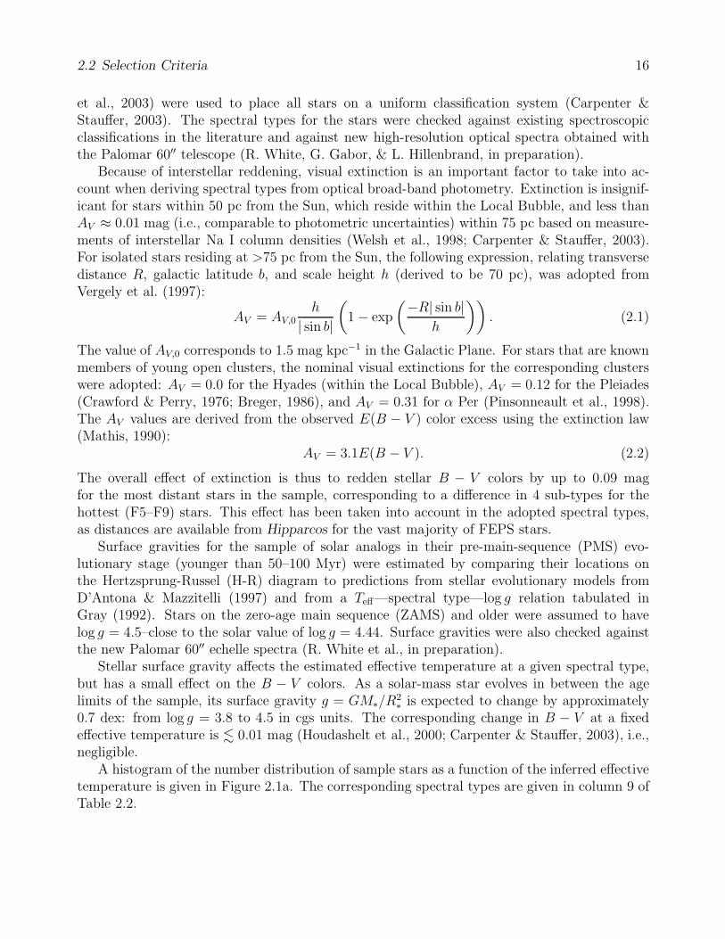
A histogram of the number distribution of sample stars as a function of the inferred effectivetemperature is given in Figure 2.1a. The corresponding spectral types are given in column 9 ofTable 2.2.
2.2 Selection Criteria 17
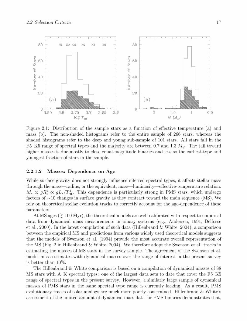
Figure 2.1: Distribution of the sample stars as a function of effective temperature (a) andmass (b). The non-shaded histograms refer to the entire sample of 266 stars, whereas theshaded histograms refer to the deep and young sub-sample of 101 stars. All stars fall in theF5–K5 range of spectral types and the majority are between 0.7 and 1.3 M. The tail towardhigher masses is due mostly to close equal-magnitude binaries and less so the earliest-type andyoungest fraction of stars in the sample.
2.2.1.2 Masses: Dependence on Age
While surface gravity does not strongly influence inferred spectral types, it affects stellar massthrough the mass—radius, or the equivalent, mass—luminosity—effective-temperature relation:M∗ ∝ gR2
∗ ∝ gL∗/T4eff . This dependence is particularly strong in PMS stars, which undergo
factors of ∼10 changes in surface gravity as they contract toward the main sequence (MS). Werely on theoretical stellar evolution tracks to correctly account for the age-dependence of theseparameters.
At MS ages (& 100 Myr), the theoretical models are well-calibrated with respect to empiricaldata from dynamical mass measurements in binary systems (e.g., Andersen, 1991; Delfosseet al., 2000). In the latest compilation of such data (Hillenbrand & White, 2004), a comparisonbetween the empirical MS and predictions from various widely used theoretical models suggeststhat the models of Swenson et al. (1994) provide the most accurate overall representation ofthe MS (Fig. 2 in Hillenbrand & White, 2004). We therefore adopt the Swenson et al. tracks inestimating the masses of MS stars in the survey sample. The agreement of the Swenson et al.model mass estimates with dynamical masses over the range of interest in the present surveyis better than 10%.
The Hillenbrand & White comparison is based on a compilation of dynamical masses of 88MS stars with A–K spectral types: one of the largest data sets to date that cover the F5–K5range of spectral types in the present survey. However, a similarly large sample of dynamicalmasses of PMS stars in the same spectral type range is currently lacking. As a result, PMSevolutionary tracks of solar analogs are much more poorly constrained. Hillenbrand & White’sassessment of the limited amount of dynamical mass data for PMS binaries demonstrates that,

2.2 Selection Criteria 18
in the 0.5–1.2 M mass range, the Baraffe et al. (1998) stellar evolution code (with the value ofthe mixing parameter α set to 1) marginally outperforms other suites of models in reproducingthe empirical data. The agreement with the dynamical masses is on average better than 10%,although with a scatter of up to 50%. Since the range of the Baraffe et al. (1998) models(0.05–1.4 M) encompasses most of the range of stellar masses (0.7–1.3 M by design) in thepresent sample, we adopt the Baraffe et al. models. For the few > 1.4M PMS sample stars,masses have been extrapolated above the 1.4 M limit of the Baraffe et al. models.
Because of the large scatter in the predictions from the PMS models, compared to the slowevolution in stellar luminosity and temperature in the final stages before reaching the ZAMS,we adopt the Baraffe et al. (1998) tracks only for stars younger than 30 Myr. For stars ≥ 30 Myrwe adopt the MS models of Swenson et al. (1994). The use of MS models to obtain masses for30–100 Myr-old stars results in a ≈10% over-estimate of the masses of the most slowly evolvingstars in the sample, the K dwarfs.
The adopted primary mass for each star is listed in the last column of Table 2.2. Thedistribution of primary masses in the full sample, and in the deep sub-sample, is plotted inFigure 2.1b. The majority of the masses are between 0.7 and 1.3 M, following the designof the FEPS sample. The tail toward high masses is almost entirely due to close equal-fluxbinaries, which were unknown as such prior to this survey. A smaller fraction of the starsmore massive than 1.3 M were among the earliest-type (F5–G0) and youngest (3 Myr) samplestars, which satisfied the spectral type selection criteria because of their youth (and hence,cooler-than-MS Teff).
The need for estimating masses for the sample stars goes beyond the original FEPS goalto focus on the evolution of solar-mass stars. We will use these masses in the context of thepresent survey in §6, when discussing the distribution of mass ratios in resolved binary systems.
2.2.2 Stellar Ages
Determination of stellar ages is done via a range of techniques all tied to the fundamentalcalibration of open and globular cluster ages that are known with respect to theoretical models.The classic method of main-sequence turn-off fitting uses the location of the giant branch turn-off on the color-magnitude diagram. The more novel method of lithium depletion boundarydetermination (Basri et al., 1996; Stauffer, 2000) estimates ages by finding the warmest fullyconvective (< 0.25M) star that still has lithium present in its photosphere. The method relieson the fact that as soon as the temperature in the contracting core of a low-mass star reacheslithium fusion values (2−4×10⁷ K), the surface lithium abundance rapidly drops to zero sincethere is no mechanism for stable lithium production.
These two methods demonstrate that stellar ages are most reliably determined in ensemblesof presumably co-eval stars with similar metallicities. They have been successfully used toage-date a large number of young open clusters (e.g., Mermilliod, 1981; Stauffer, 2000, andreferences therein). For the sample stars that are known members of these clusters, we haveadopted the corresponding ages: 5 ± 1 Myr for the Upper Scorpius OB association (Preibischet al., 2002), 90±10 Myr for α Per (Stauffer et al., 1999), 125±8 Myr for the Pleiades (Staufferet al., 1998), and 625 ± 50 Myr for the Hyades (Perryman et al., 1998).
The two primary methods for estimating stellar ages of clusters have allowed the calibrationof a number of secondary empirical relations, suitable for age-dating individual field stars. Mostnotable among the secondary methods are ones based on the evolution of the stellar dynamo,

2.2 Selection Criteria 19
on the surface lithium abundance in stars with convective envelopes (but radiative cores), andon the “memory” of a star’s space motion after leaving its molecular cloud progenitor. Sincethe majority of the stars in the sample are not members of young open clusters, age-dating ofthe sample relies heavily on these secondary techniques.
The full set of age indicators used were the following:
1. location on the H-R diagram in relation to stellar populations of known age and to theo-retical evolutionary tracks, a.k.a. “isochrone fitting”;
2. chromospheric Ca II H and K (3968 and 3933A) line emission;
3. chromospheric Hα emission;
4. chromospheric UV continuum excess and line emission;
5. coronal x-ray emission;
6. rotation velocity v sin i, as measured from rotational line broadening;
7. Li I 6707A absorption;
8. UVW galactic space motion.
Comprehensive discussions of the above age indicators and their advantages and limitationscan be found in Gaidos (1998) and Lachaume et al. (1999). Their application to age-datingthe FEPS sample is detailed in Hillenbrand et al. (2005, and references therein). Here, wepresent only a brief description of each method. It is important to note that because of thelarger uncertainties of the secondary age-dating methods compared to the primary ones, severalsecondary methods need to be used in conjunction for reliable age estimation.
The first technique is similar in spirit to the main-sequence turn-off fitting, in the sensethat it uses theoretical and empirical isochrones. However, unlike the evolved stars on themain-sequence turn-off, for the young solar analogs in the FEPS sample (whose distances areknown; §2.2.3), location above the ZAMS in the H-R diagram is an indication of youth, ratherthan old age. Whether this is truly the case is confirmed by some of the other methods. If thestar is confirmed to be young, its age can be determined fairly precisely from PMS contractiontracks. The method is not suitable for age-dating stars on the MS (i.e., > 100 Myr-old G stars)because of the very slow evolution of temperature and luminosity. Only a lower limit on theage can be established for such stars.
The MKSvs. J − KS plot in Figure 2.2 shows an example of the H-R diagram dating
technique, as applied to the AO survey sample, based on models from Baraffe et al. (1998).Isochrones are plotted in continuous lines, while lines of constant mass are shown in dashedlines. The majority of the sample stars cluster near the 100 Myr (≈ZAMS) isochrone, indicatingthat their ages are &100 Myr. The stars scattered above the 100 Myr isochrone are accordinglyyounger. This particular set of evolutionary tracks (with α = 1.0) from Baraffe et al. over-predicts the luminosity of the ZAMS by ∆MKS
≈ 0.3 mag. Such a discrepancy is not unusualfor theoretical PMS models. In this case, the discrepancy can be largely eliminated by adoptinga different set of evolutionary tracks from the same authors, with the value of the mixing-scaleparameter α set to 1.9. This is the setting required to reproduce the present Sun in the (Baraffeet al., 1998) suite of models. However, as already discussed in §2.2.1.2, the α = 1.0 models

2.2 Selection Criteria 20
Figure 2.2: MKSvs. J−KS color-magnitude diagram of the AO survey sample with evolutionary
tracks from Baraffe et al. (1998) over-plotted. Continuous curves delineate isochrones anddashed curves delineate tracks of constant mass. The vector at the bottom left represents theequivalent of 1 magnitude of V -band extinction. The apparent ∆MKS
≈ 0.3 mag displacementof the 100 Myr (approximately ZAMS) isochrone from the locus of the majority of the stars isan example of the uncertainties in theoretical models.
were found to best approximate the masses of <30 Myr PMS stars on average, and are hencethe choice of models for young PMS stars in this study.
Age-dating methods (2–6) are related to the evolution of the stellar dynamo. A relationshipbetween rotation and dynamo-driven activity is expected theoretically, based on the conversionof mechanical to magnetic energy, though the calibration to stellar age is derived from empiricalcorrelations of observed quantities. Such observational correlations were first presented in abrief paper by Skumanich (1972), who observed that the decay of chromospheric emission androtational velocity among stars in different young open clusters varies as the inverse square rootof cluster age. Subsequent more-detailed analyses of the evolution of rotation velocity, v sin i(Soderblom, 1983), x-ray coronal luminosity (Vilhu, 1984; Randich, 2000), and chromosphericUV, Ca II H&K, and Hα emission (e.g., Simon et al., 1985; Donahue, 1993; Lyra & Porto deMello, 2005), have established a variety of empirical laws suitable for determining approximatestellar ages in the 30–5000 Myr range. Best calibrated and most widely used among theseage indicators is the R′
HK index, measuring the relative strength of Ca II H&K emission with

2.2 Selection Criteria 21
respect to the stellar continuum (Noyes et al., 1984). This we adopt as the primary criterionfor determining ages for post-PMS stars. Quantitatively, we employ the following empiricalrelation from (Donahue, 1993):
log
(
t
year
)
= 10.725 − 1.334R5 + 0.4085R25 − 0.0522R3
5, (2.3)
where t is the stellar age in years and R5 = 105R′HK . The observational scatter in the above
relation has been estimated at ≤50% based on variations in the derived ages of the componentsof binaries, which can be assumed to be co-eval (Donahue, 1998). Where available, R′
HK
measurements for the sample stars are listed in column 10 of Table 2.2.The seventh method relies on the fact that as low-mass stars with radiative cores age,
lithium is gradually mixed downward in the convective envelope until reaching the temperatureat which it burns. Therefore, assuming that all stars start with primordial lithium abundances,presence of photospheric lithium is an indication of youth (e.g., Herbig, 1965; Bodenheimer,1965; Duncan, 1981). While the equivalent width of the Li I 6707A absorption resonancedoublet (the strongest lithium feature in the optical) is not a direct measure of the absolutelithium abundance, its relative strength in populations of stars of similar temperature can beused to qualitatively compare their ages. However, the large observational scatter in lithiumfor stars of similar temperature and age, especially for G stars (e.g., Duncan & Jones, 1983),precludes its use as an absolute chronometer, only a statistical one.
Finally, method (8) presents a statistical approach for selecting groups of co-eval co-movingstars. The underlying idea, originally due to Eggen (1965), is that stars are born in groupsand are imprinted with the space motion of the parent molecular cloud even after escapingits gravitational influence. The method of calculating space motions in the Galactic (U, V,W )coordinate system from the celestial coordinates, parallax, radial velocity, and proper motionwas standardized by Johnson & Soderblom (1987). Leggett (1992) defined criteria for assigningmembership to the young disk, the old disk, or the halo of the Galaxy, representing young,intermediate-aged, and old stars. Thus, while the space motion of a star has no formulaicrelation to its age, it can be compared to the space motions of ensembles of stars of knownage, thus revealing tentative associations of young stars spread over the entire sky. However,confirmation of youth through one or more of the aforementioned methods is essential. Acompilation of known and tentative young moving groups and their space motions is presentedin Zuckerman & Song (2004b).
To summarize, ages for the sample solar analogs were determined based on two primarymethods: isochrone fitting of the location on the H-R diagram for <30 Myr PMS stars (method1) and strength of the R′
HK chromospheric activity index for older stars (method 2). The othertechniques were applied where possible and necessary to confirm and further constrain thestellar ages. Histograms of the age distribution of the complete survey sample and of the deepsub-sample are presented in Figure 2.3. The determined stellar ages will be used in §6 and 6to determine age-dependent masses for candidate and bona fide sub-stellar companions. Theadopted ages for the sample stars are listed in column 12 of Table 2.2.

2.2 Selection Criteria 22
Figure 2.3: Age distributions of the complete survey sample (non-shaded histogram) and of thedeep sub-sample (shaded histogram).
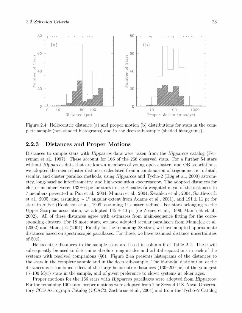
2.2 Selection Criteria 23
Figure 2.4: Heliocentric distance (a) and proper motion (b) distributions for stars in the com-plete sample (non-shaded histograms) and in the deep sub-sample (shaded histograms).
2.2.3 Distances and Proper Motions
Distances to sample stars with Hipparcos data were taken from the Hipparcos catalog (Per-ryman et al., 1997). These account for 166 of the 266 observed stars. For a further 54 starswithout Hipparcos data that are known members of young open clusters and OB associations,we adopted the mean cluster distance, calculated from a combination of trigonometric, orbital,secular, and cluster parallax methods, using Hipparcos and Tycho-2 (Høg et al., 2000) astrom-etry, long-baseline interferometry, and high-resolution spectroscopy. The adopted distances forcluster members were: 133±6 pc for stars in the Pleiades (a weighted mean of the distances to7 members presented in Pan et al., 2004, Munari et al., 2004, Zwahlen et al., 2004, Southworthet al., 2005, and assuming ∼ 1 angular extent from Adams et al., 2001), and 191 ± 11 pc forstars in α Per (Robichon et al., 1999, assuming 1 cluster radius). For stars belonging to theUpper Scorpius association, we adopted 145 ± 40 pc (de Zeeuw et al., 1999; Mamajek et al.,2002). All of these distances agree with estimates from main-sequence fitting for the corre-sponding clusters. For 18 more stars, we have adopted secular parallaxes from Mamajek et al.(2002) and Mamajek (2004). Finally for the remaining 28 stars, we have adopted approximatedistances based on spectroscopic parallaxes. For these, we have assumed distance uncertaintiesof 50%.
Heliocentric distances to the sample stars are listed in column 6 of Table 2.2. These willsubsequently be used to determine absolute magnitudes and orbital separations in each of thesystems with resolved companions (§6). Figure 2.4a presents histograms of the distances tothe stars in the complete sample and in the deep sub-sample. The bi-modal distribution of thedistances is a combined effect of the large heliocentric distances (130–200 pc) of the youngest(5–100 Myr) stars in the sample, and of given preference to closer systems at older ages.
Proper motions for the 166 stars with Hipparcos parallaxes were adopted from Hipparcos.For the remaining 100 stars, proper motions were adopted from The Second U.S. Naval Observa-tory CCD Astrograph Catalog (UCAC2; Zacharias et al., 2004) and from the Tycho–2 Catalog

2.3 Sample Selection 24
(Høg et al., 2000). The three catalogs provided similar astrometric accuracy (±1.0 mas yr−1)for the sample stars, though the UCAC2 and Tycho–2 catalogs went deeper. The proper motionalong right ascension (corrected for declination: µα cos δ) and declination (µδ) for each star isgiven in columns 4 and 5 of Table 2.2.
The distribution of the total (√
(µα cos δ)2 + µ2δ) proper motions for the sample stars is
presented in Figure 2.4b. The proper motions of the sample stars will be essential in identifyingbona fide companions to the sample stars through astrometry (§5).
2.3 Sample Selection
The description of the sample selection process presented in §2.3.1 is a summary of the algorithmemployed for the FEPS sample selection, discussed in greater detail by Meyer et al. (2005). Thelimited number of target additions and further constraints are discussed in §2.3.2.
2.3.1 FEPS Sample Selection
The stars in the FEPS target list are drawn from three recently assembled compilations ofsolar analogs. The first compilation is that of Soderblom et al. (2000, private communication),who have produced a volume-limited (based on Hipparcos) set of approximately 5000 solar-type stars over the entire sky. The Soderblom et al. sample exhibits some overlap with therecently published Wright et al. (2004) sample, which will henceforth be used as the referenceof choice. The stars in this sample have parallaxes that place them within 60 pc, B − V colorsbetween 0.52 mag and 0.81 mag (F8–K0 spectral types), and location on the H-R diagramwithin 1.0 mag of the solar-metallicity ZAMS. The sample is fully complete to 50 pc. Fromthis sample, the FEPS team has extracted stars with ages between 0.1 and 3 Gyr, based on theR′HK chromospheric activity index (§2.2.2). However, being located more than 100 pc from the
nearest star-forming region, the Soderblom et al. list is deficient in stars younger than a fewhundred Myr.
To fill in the gap at young ages, the volume limit was extended to include large enoughsamples of young stars. These were identified from new spectroscopic observations of x-rayand proper-motion-selected samples of late-type stars (e.g., Mamajek et al., 2002), and from anexamination of the literature. The surface density distribution of x-ray sources in the ROSATall-sky survey reveals a concentration of objects coincident with Gould’s Belt: an expandingring of atomic and molecular gas in the distant solar neighborhood (50–200 pc), which comprisesnearly all star-forming regions within 1 kpc. Tycho-2 proper motion data allow the selectionof the nearest of these x-ray emitting stars with space motions consistent with those of higher-mass, young stars with measured parallaxes. As in the case of the <50 pc sample, the youthof the stars is confirmed from follow-up high-resolution spectroscopic observations. There areapproximately 600 stars in this sample, ranging from 3 to 100 Myr in age, with B − V colorsbetween 0.58 and 1.20 (spectral types G0–K5), strong x-ray emission, kinematics appropriatefor the young galactic disk, and high lithium abundance compared to the 125 Myr old Pleiades.
Finally, all known members of nearby well-studied young open clusters (IC 2602, α Per, thePleiades, and the Hyades) meeting the targeted spectral type range were also considered.
From this large sample, targets were selected for the FEPS Spitzer campaign if they met allof the following criteria (Meyer et al., 2005):
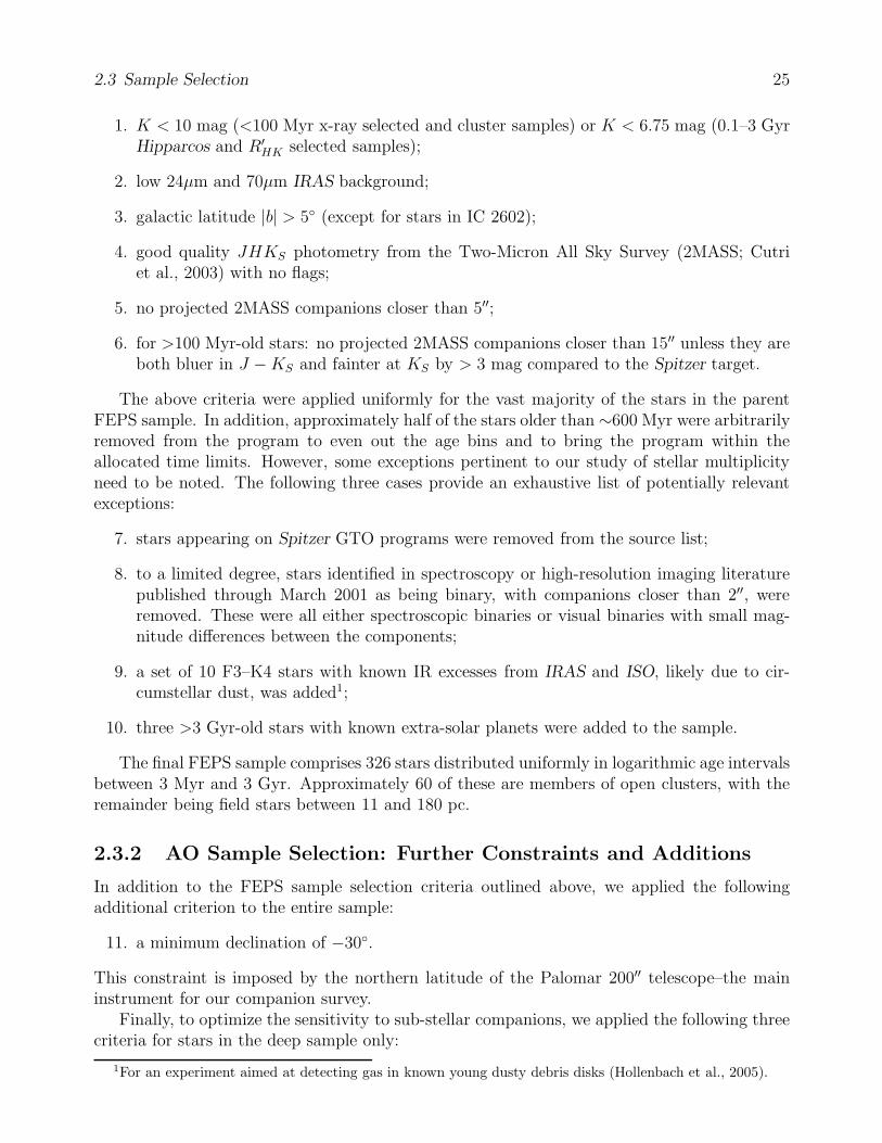
2.3 Sample Selection 25
1. K < 10 mag (<100 Myr x-ray selected and cluster samples) or K < 6.75 mag (0.1–3 GyrHipparcos and R′
HK selected samples);
2. low 24µm and 70µm IRAS background;
3. galactic latitude |b| > 5 (except for stars in IC 2602);
4. good quality JHKS photometry from the Two-Micron All Sky Survey (2MASS; Cutriet al., 2003) with no flags;
5. no projected 2MASS companions closer than 5′′;
6. for >100 Myr-old stars: no projected 2MASS companions closer than 15′′ unless they areboth bluer in J −KS and fainter at KS by > 3 mag compared to the Spitzer target.
The above criteria were applied uniformly for the vast majority of the stars in the parentFEPS sample. In addition, approximately half of the stars older than ∼600 Myr were arbitrarilyremoved from the program to even out the age bins and to bring the program within theallocated time limits. However, some exceptions pertinent to our study of stellar multiplicityneed to be noted. The following three cases provide an exhaustive list of potentially relevantexceptions:
7. stars appearing on Spitzer GTO programs were removed from the source list;
8. to a limited degree, stars identified in spectroscopy or high-resolution imaging literaturepublished through March 2001 as being binary, with companions closer than 2′′, wereremoved. These were all either spectroscopic binaries or visual binaries with small mag-nitude differences between the components;
9. a set of 10 F3–K4 stars with known IR excesses from IRAS and ISO, likely due to cir-cumstellar dust, was added1;
10. three >3 Gyr-old stars with known extra-solar planets were added to the sample.
The final FEPS sample comprises 326 stars distributed uniformly in logarithmic age intervalsbetween 3 Myr and 3 Gyr. Approximately 60 of these are members of open clusters, with theremainder being field stars between 11 and 180 pc.
2.3.2 AO Sample Selection: Further Constraints and Additions
In addition to the FEPS sample selection criteria outlined above, we applied the followingadditional criterion to the entire sample:
11. a minimum declination of −30.
This constraint is imposed by the northern latitude of the Palomar 200′′ telescope–the maininstrument for our companion survey.
Finally, to optimize the sensitivity to sub-stellar companions, we applied the following threecriteria for stars in the deep sample only:
1For an experiment aimed at detecting gas in known young dusty debris disks (Hollenbach et al., 2005).
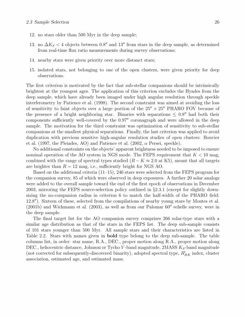
2.3 Sample Selection 26
12. no stars older than 500 Myr in the deep sample;
13. no ∆KS < 4 objects between 0.8′′ and 13′′ from stars in the deep sample, as determinedfrom real-time flux ratio measurements during survey observations;
14. nearby stars were given priority over more distanct stars;
15. isolated stars, not belonging to one of the open clusters, were given priority for deepobservations.
The first criterion is motivated by the fact that sub-stellar companions should be intrinsicallybrightest at the youngest ages. The application of this criterion excludes the Hyades from thedeep sample, which have already been imaged under high angular resolution through speckleinterferometry by Patience et al. (1998). The second constraint was aimed at avoiding the lossof sensitivity to faint objects over a large portion of the 25′′ × 25′′ PHARO FOV because ofthe presence of a bright neighboring star. Binaries with separations ≤ 0.8′′ had both theircomponents sufficiently well-covered by the 0.97′′ coronagraph and were allowed in the deepsample. The motivation for the third constraint was optimization of sensitivity to sub-stellarcompanions at the smallest physical separations. Finally, the last criterion was applied to avoidduplication with previous sensitive high-angular resolution studies of open clusters: Bouvieret al. (1997, the Pleiades, AO) and Patience et al. (2002, α Persei, speckle).
No additional constraints on the objects’ apparent brightness needed to be imposed to ensurenominal operation of the AO system in NGS mode. The FEPS requirement that K < 10 mag,combined with the range of spectral types studied (R−K ≈ 2.0 at K5), meant that all targetsare brighter than R = 12 mag, i.e., sufficiently bright for NGS AO.
Based on the additional criteria (11–15), 246 stars were selected from the FEPS program forthe companion survey, 85 of which were observed in deep exposures. A further 20 solar analogswere added to the overall sample toward the end of the first epoch of observations in December2003, mirroring the FEPS source-selection policy outlined in §2.3.1 (except for slightly down-sizing the no-companion radius in criterion 6 to match the half-width of the PHARO field:12.8′′). Sixteen of these, selected from the compilations of nearby young stars by Montes et al.(2001b) and Wichmann et al. (2003), as well as from our Palomar 60′′ echelle survey, were inthe deep sample.
The final target list for the AO companion survey comprises 266 solar-type stars with asimilar age distribution as that of the stars in the FEPS list. The deep sub-sample consistsof 101 stars younger than 500 Myr. All sample stars and their characteristics are listed inTable 2.2. Stars with names given in bold type belong to the deep sub-sample. The tablecolumns list, in order: star name, R.A., DEC., proper motion along R.A., proper motion alongDEC., heliocentric distance, Johnson or Tycho V -band magnitude, 2MASS KS-band magnitude(not corrected for subsequently-discovered binarity), adopted spectral type, R′
HK index, clusterassociation, estimated age, and estimated mass.

2.3Sam
ple
Selection
27
Table 2.2: Survey SampleStar α δ µα cos δ µdelta d V or VT KS Sp.T. R′
HKAssoc. Age M
(J2000.0) (J2000.0) (mas yr−1) (mas yr−1) (pc) (mag) (mag) (log Myr−1) (M)
HD 224873 00:01:23.66 +39:36:38.12 −28.7 ± 0.6 −43.3 ± 0.7 49.0 ± 5.0 8.6 6.7 K0 –4.38 · · · 8.48+0.30
−0.301.01
HD 377 00:08:25.74 +06:37:00.50 85.2 ± 1.5 −2.6 ± 1.4 40.0 ± 2.0 7.6 6.1 G2V –4.29 · · · 7.59+0.30
−0.301.11
HD 691 00:11:22.44 +30:26:58.52 209.7 ± 1.0 35.5 ± 1.0 34.0 ± 1.0 8.0 6.2 K0V –4.38 · · · 8.46+0.30
−0.300.98
HD 984 00:14:10.25 –07:11:56.92 104.9 ± 1.3 −67.6 ± 1.2 46.0 ± 2.0 7.4 6.1 F7V –4.29 · · · 7.63+0.30
−0.301.22
HD 1405 00:18:20.78 +30:57:23.76 141.5 ± 2.2 −177.0 ± 2.1 29.0 ± 10.0 8.6 6.4 K2V –5.18 · · · 8.00+0.30
−0.300.84
QT And 00:41:17.32 +34:25:16.77 44.8 ± 0.7 −36.2 ± 0.8 50.0 ± 25.0 10.1 7.3 K4 · · · · · · 7.79 ± 0.29 0.84
HD 6963 01:10:41.91 +42:55:54.50 −154.6 ± 0.9 −198.5 ± 0.9 27.0 ± 1.0 7.7 5.9 G7V –4.54 · · · 9.02+0.30
−0.300.93
HD 7661 01:16:24.19 –12:05:49.33 134.8 ± 1.1 −5.7 ± 1.1 27.0 ± 1.0 7.6 5.7 K0V –4.41 · · · 8.64+0.30
−0.300.96
HIP 6276 01:20:32.27 –11:28:03.74 116.0 ± 1.1 −140.2 ± 1.1 35.0 ± 1.0 8.5 6.5 G0 –4.38 · · · 8.47+0.30
−0.300.91
HD 8467 01:24:28.00 +39:03:43.55 210.6 ± 1.8 −26.6 ± 1.0 31.0 ± 1.0 8.5 6.6 G5 –4.74 · · · 9.33 ± 0.30 0.82
HD 8941 01:28:24.36 +17:04:45.20 118.3 ± 0.7 −34.8 ± 0.7 50.0 ± 2.0 6.6 5.4 F8IV–V –4.66 · · · 9.22+0.30
−0.301.46
HD 8907 01:28:34.35 +42:16:03.70 51.7 ± 1.0 −99.2 ± 1.1 34.0 ± 1.0 6.6 5.4 F8 –4.39 · · · 8.25 ± 0.25 1.23
HD 9472 01:33:19.03 +23:58:32.19 0.0 ± 1.0 28.4 ± 0.9 33.0 ± 1.0 7.7 6.0 G0 –4.49 · · · 8.93+0.30
−0.301.02
RE J0137+18A 01:37:39.41 +18:35:33.16 65.8 ± 1.9 −46.0 ± 2.5 64.0 ± 8.0 10.7 6.7 K3Ve · · · · · · 6.75 ± 0.25 1.02
HD 11850 01:56:47.27 +23:03:04.09 −83.8 ± 1.0 −18.1 ± 1.0 33.0 ± 1.0 7.9 6.2 G5 –4.44 · · · 8.76+0.30
−0.300.98
HD 12039 01:57:48.98 –21:54:05.32 102.4 ± 1.2 −48.0 ± 1.1 42.0 ± 2.0 8.1 6.5 G3/5V –4.21 · · · 7.50 ± 0.30 0.98
HD 13382 02:11:23.15 +21:22:38.39 273.1 ± 0.8 −12.6 ± 0.7 33.0 ± 1.0 7.4 5.8 G5V –4.42 · · · 8.71+0.30
−0.301.08
HD 13507 02:12:55.00 +40:40:06.00 56.9 ± 1.3 −99.2 ± 1.3 26.0 ± 1.0 7.2 5.6 G5V –4.48 · · · 8.89+0.30
−0.301.00
HD 13531 02:13:13.35 +40:30:27.34 57.6 ± 1.0 −96.4 ± 1.0 26.0 ± 1.0 7.4 5.7 G7V –4.42 · · · 8.67+0.30
−0.300.98
HD 13974 02:17:03.23 +34:13:27.32 1153.8 ± 0.8 −245.1 ± 0.8 11.0 ± 0.1 4.8 3.2 G0V –4.64 · · · 9.19+0.30
−0.301.10
HD 15526 02:29:35.03 –12:24:08.56 42.1 ± 1.3 −12.2 ± 1.1 106.0 ± 26.0 9.9 8.0 G5/6V · · · · · · 7.62 ± 0.12 1.131RXS J025216.9+361658 02:52:17.59 +36:16:48.14 53.4 ± 1.3 −40.1 ± 0.7 140.0 ± 70.0 10.7 7.6 K2IV · · · · · · 7.75 ± 0.25 1.111RXS J025223.5+372914 02:52:24.73 +37:28:51.83 22.5 ± 0.7 −24.5 ± 1.0 170.0 ± 85.0 10.8 9.1 G5IV · · · · · · 8.25 ± 0.25 1.16HD 17925 02:52:32.14 –12:46:11.18 397.3 ± 1.2 −189.9 ± 1.3 10.0 ± 0.1 6.0 4.1 K1V –4.311 · · · 7.87 ± 0.13 0.862RE J0255+474 02:55:43.60 +47:46:47.58 79.8 ± 0.6 −76.1 ± 0.7 50.0 ± 25.0 10.8 7.2 K5Ve · · · αPer 7.90 ± 0.15 0.821RXS J025751.8+115759 02:57:51.68 +11:58:05.83 31.4 ± 1.2 −28.4 ± 1.2 118.0 ± 16.0 10.8 8.5 G7V · · · · · · 7.75 ± 0.25 1.05RX J0258.4+2947 02:58:28.77 +29:47:53.80 17.4 ± 1.2 −40.0 ± 0.6 100.0 ± 50.0 11.4 9.1 K0IV · · · · · · 8.00 ± 0.10 0.86
HD 18940 03:03:28.65 +23:03:41.19 111.4 ± 0.8 −0.7 ± 0.7 34.0 ± 1.0 7.1 5.5 G0 –4.47 · · · 8.87+0.30
−0.301.15
HD 19019 03:03:50.82 +06:07:59.82 231.8 ± 1.8 50.7 ± 1.7 31.0 ± 1.0 7.0 5.6 F8 –4.62 · · · 9.16 ± 0.30 1.131RXS J030759.1+302032 03:07:59.20 +30:20:26.05 31.2 ± 0.6 −66.6 ± 0.7 75.0 ± 37.5 9.3 7.4 G5IV · · · · · · 8.25 ± 0.25 1.08
continued on next page
2.3Sam
ple
Selection
28Table 2.2 – continued from previous page
Star α δ µα cos δ µdelta d V or VT KS Sp.T. R′HK
Assoc. Age M
(J2000.0) (J2000.0) (mas yr−1) (mas yr−1) (pc) (mag) (mag) (log Myr−1) (M)
HD 19632 03:08:52.45 –24:53:15.55 226.7 ± 1.3 136.3 ± 1.3 30.0 ± 1.0 7.4 5.7 G3/5V –4.40 · · · 8.60+0.30
−0.301.07
HD 19668 03:09:42.28 –09:34:46.46 88.0 ± 1.2 −113.3 ± 1.1 40.0 ± 2.0 8.6 6.7 G8/K0V –4.36 · · · 8.36+0.30
−0.300.94
1E 0307.4+1424 03:10:12.55 +14:36:02.90 −4.0 ± 1.2 −25.3 ± 1.2 160.0 ± 80.0 10.5 8.8 G6V · · · · · · 7.75 ± 0.25 1.15
vB 1 03:17:26.39 +07:39:20.90 167.2 ± 1.3 −6.4 ± 1.4 43.1 ± 0.6 7.4 6.0 F8 –4.60 Hyades 8.78+0.30
−0.301.18
HE 350 03:17:36.93 +48:50:08.50 23.2 ± 0.8 −23.0 ± 0.9 190.0 ± 11.0 11.1 9.3 G2 · · · αPer 7.90+0.30
−0.301.22
HE 373 03:18:27.39 +47:21:15.42 29.0 ± 0.7 −26.8 ± 2.0 190.0 ± 11.0 11.5 9.4 G8 · · · αPer 7.90+0.30
−0.301.21
HE 389 03:18:50.31 +49:43:52.19 22.5 ± 0.9 −23.9 ± 0.7 190.0 ± 11.0 11.2 9.5 G0 · · · αPer 7.90+0.30
−0.301.13
AP 93 03:19:02.76 +48:10:59.61 16.4 ± 4.0 −23.6 ± 1.4 190.0 ± 11.0 12.0 9.4 K2 · · · αPer 7.90+0.30
−0.301.00
1RXS J031907.4+393418 03:19:07.61 +39:34:10.50 27.3 ± 0.9 −25.3 ± 1.7 100.0 ± 50.0 11.7 9.5 K0V · · · · · · 7.75 ± 0.25 0.79
HE 622 03:24:49.71 +48:52:18.33 22.3 ± 0.9 −26.3 ± 0.7 190.0 ± 11.0 11.7 9.6 G7 · · · αPer 7.90+0.30
−0.301.06
HE 696 03:26:19.36 +49:13:32.54 19.8 ± 0.7 −25.0 ± 0.7 190.0 ± 11.0 11.6 9.7 G3 · · · αPer 7.90+0.30
−0.301.03
1E 0324.1–2012 03:26:22.05 –20:01:48.81 25.0 ± 1.6 7.4 ± 1.6 160.0 ± 80.0 10.4 8.9 G4V · · · · · · 7.75 ± 0.25 1.15
HE 699 03:26:22.22 +49:25:37.52 22.4 ± 0.8 −24.5 ± 0.7 190.0 ± 11.0 11.3 9.4 G3 · · · αPer 7.90+0.30
−0.301.12
HE 750 03:27:37.79 +48:59:28.78 22.0 ± 0.7 −25.6 ± 0.7 190.0 ± 11.0 10.5 9.1 F5 · · · αPer 7.90+0.30
−0.301.21
HE 767 03:27:55.02 +49:45:37.16 21.1 ± 0.6 −26.0 ± 0.6 190.0 ± 11.0 10.7 9.2 F6 · · · αPer 7.90+0.30
−0.301.23
RX J0329.1+0118 03:29:08.06 +01:18:05.66 4.4 ± 1.3 −4.5 ± 1.3 100.0 ± 50.0 10.6 9.2 G0(IV) · · · · · · 7.75 ± 0.25 0.91
HE 848 03:29:26.24 +48:12:11.74 22.2 ± 0.6 −26.4 ± 0.6 190.0 ± 11.0 10.0 8.5 F9V · · · αPer 7.90+0.30
−0.301.33
HE 935 03:31:28.99 +48:59:28.37 21.3 ± 0.9 −26.6 ± 0.6 190.0 ± 11.0 10.1 8.5 F9.5V · · · αPer 7.90+0.30
−0.301.33
HE 1101 03:35:08.75 +49:44:39.59 20.9 ± 1.3 −28.5 ± 0.9 190.0 ± 11.0 11.3 9.3 G5 · · · αPer 7.90+0.30
−0.301.18
HD 22179 03:35:29.91 +31:13:37.45 42.6 ± 0.6 −46.0 ± 0.7 140.0 ± 70.0 9.0 7.4 G5IV · · · · · · 7.75 ± 0.25 1.26
HE 1234 03:39:02.91 +51:36:37.11 21.4 ± 0.8 −33.7 ± 0.7 190.0 ± 11.0 10.8 8.9 G4 · · · αPer 7.90+0.30
−0.301.27
HD 22879 03:40:22.08 –03:13:00.86 691.6 ± 1.1 −212.8 ± 1.1 24.0 ± 1.0 6.7 5.2 F7/8V –4.71 · · · 9.29+0.30
−0.300.79
HD 23208 03:42:39.80 –20:32:43.80 3.8 ± 1.4 24.1 ± 1.0 57.5 ± 4.7 9.2 7.2 G8V –5.18 · · · 6.70 ± 0.30 0.61
HII 102 03:43:24.54 +23:13:33.30 17.1 ± 0.6 −43.7 ± 0.6 133.0 ± 6.0 10.5 8.7 G6 · · · Pleiades 8.08+0.30
−0.301.12
HII 120 03:43:31.95 +23:40:26.61 18.0 ± 0.7 −46.8 ± 0.6 133.0 ± 6.0 10.8 9.1 G5 · · · Pleiades 8.08+0.30
−0.301.05
HII 152 03:43:37.73 +23:32:09.59 19.5 ± 0.7 −46.9 ± 1.0 133.0 ± 6.0 10.7 9.1 G4 · · · Pleiades 8.08+0.30
−0.301.01
HII 174 03:43:48.33 +25:00:15.83 18.8 ± 1.1 −47.0 ± 0.9 133.0 ± 6.0 11.6 9.4 K1 · · · Pleiades 8.08+0.30
−0.300.90
HII 173 03:43:48.41 +25:11:24.19 20.4 ± 0.8 −48.4 ± 0.7 133.0 ± 6.0 10.9 8.8 K0 · · · Pleiades 8.08+0.30
−0.301.06
HII 250 03:44:04.24 +24:59:23.40 20.1 ± 1.0 −49.4 ± 0.7 133.0 ± 6.0 10.7 9.1 G3 · · · Pleiades 8.08+0.30
−0.301.04
HII 314 03:44:20.09 +24:47:46.16 18.2 ± 0.7 −49.8 ± 0.8 133.0 ± 6.0 10.6 8.9 G3 · · · Pleiades 8.08+0.30
−0.301.13
1RXS J034423.3+281224 03:44:24.25 +28:12:23.07 46.4 ± 0.7 −50.6 ± 0.6 100.0 ± 50.0 8.9 7.2 G7V · · · · · · 7.75 ± 0.25 1.30
HII 514 03:45:04.01 +25:15:28.23 17.3 ± 0.7 −46.3 ± 0.6 133.0 ± 6.0 10.7 9.0 G4 · · · Pleiades 8.08+0.30
−0.301.08
HII 571 03:45:15.35 +25:17:22.11 15.1 ± 0.9 −48.5 ± 0.9 133.0 ± 6.0 11.3 9.2 G9 · · · Pleiades 8.08+0.30
−0.300.96
HII 1015 03:46:27.35 +25:08:07.97 18.6 ± 0.7 −48.5 ± 0.9 133.0 ± 6.0 10.5 9.0 G1 · · · Pleiades 8.08+0.30
−0.301.08
HII 1101 03:46:38.78 +24:57:34.61 18.4 ± 0.8 −48.1 ± 0.7 133.0 ± 6.0 10.3 8.8 G4 · · · Pleiades 8.08+0.30
−0.301.10
HII 1182 03:46:47.06 +22:54:52.48 18.4 ± 0.6 −45.6 ± 0.7 133.0 ± 6.0 10.5 8.9 G1 · · · Pleiades 8.08+0.30
−0.301.09
HII 1200 03:46:50.54 +23:14:21.06 17.3 ± 0.6 −40.2 ± 0.7 133.0 ± 6.0 9.9 8.5 F6 · · · Pleiades 8.08+0.30
−0.301.25
HII 1348† 03:47:18.04 +24:23:27.00 14.1 ± 0.5 −48.8 ± 0.5 133.0 ± 6.0 12.1 9.7 K5 –5.18 Pleiades 8.08+0.30
−0.300.86
HII 1776 03:48:17.70 +25:02:52.29 19.0 ± 1.0 −47.1 ± 1.0 133.0 ± 6.0 11.0 9.2 G5 · · · Pleiades 8.08+0.30
−0.301.02
HII 2106 03:48:58.49 +23:12:04.33 16.5 ± 1.3 −44.9 ± 1.1 133.0 ± 6.0 11.5 9.4 K1 · · · Pleiades 8.08+0.30
−0.300.91
RX J0348.9+0110 03:48:58.76 +01:10:53.99 35.1 ± 1.6 −22.1 ± 1.2 100.0 ± 50.0 10.6 8.3 K3(V)/E · · · · · · 8.18+0.30
−0.301.05
HII 2147 03:49:06.11 +23:46:52.49 15.9 ± 0.9 −43.8 ± 0.8 133.0 ± 6.0 10.8 8.6 G7IV · · · Pleiades 8.08+0.30
−0.301.11
HII 2278 03:49:25.70 +24:56:15.43 18.4 ± 0.9 −47.0 ± 0.8 133.0 ± 6.0 10.9 8.8 K0 · · · Pleiades 8.08+0.30
−0.301.09
HII 2506 03:49:56.49 +23:13:07.01 17.6 ± 0.7 −43.9 ± 0.6 133.0 ± 6.0 10.2 8.8 F9 · · · Pleiades 8.08+0.30
−0.301.15
HII 2644 03:50:20.90 +24:28:00.22 19.8 ± 0.8 −46.8 ± 0.9 133.0 ± 6.0 11.1 9.3 G5 · · · Pleiades 8.08+0.30
−0.300.98
1RXS J035028.0+163121 03:50:28.40 +16:31:15.19 26.2 ± 1.3 −23.4 ± 2.1 138.0 ± 21.0 10.6 8.6 G5IV · · · · · · 7.75 ± 0.25 1.12
HII 2786 03:50:40.08 +23:55:58.94 17.6 ± 0.7 −45.2 ± 1.0 133.0 ± 6.0 10.3 8.9 F9 · · · Pleiades 8.08+0.30
−0.301.12
HII 2881 03:50:54.32 +23:50:05.52 17.7 ± 0.7 −46.9 ± 1.1 133.0 ± 6.0 11.6 9.1 K2 · · · Pleiades 8.08+0.30
−0.300.93
continued on next page

2.3Sam
ple
Selection
29Table 2.2 – continued from previous page
Star α δ µα cos δ µdelta d V or VT KS Sp.T. R′HK
Assoc. Age M
(J2000.0) (J2000.0) (mas yr−1) (mas yr−1) (pc) (mag) (mag) (log Myr−1) (M)
HII 3097 03:51:40.44 +24:58:59.41 17.5 ± 0.7 −46.1 ± 1.0 133.0 ± 6.0 11.0 9.1 G6 · · · Pleiades 8.08+0.30
−0.301.05
HII 3179 03:51:56.86 +23:54:06.98 19.2 ± 0.6 −46.5 ± 0.8 133.0 ± 6.0 10.0 8.6 F8 · · · Pleiades 8.08+0.30
−0.301.21
RX J0354.4+0535 03:54:21.31 +05:35:40.77 −1.4 ± 1.3 −7.6 ± 1.3 100.0 ± 50.0 10.2 8.7 G2(V) · · · · · · 8.25 ± 0.25 0.99
Pels 191 03:54:25.23 +24:21:36.38 17.1 ± 0.7 −46.8 ± 0.8 133.0 ± 6.0 11.1 9.1 G5IV · · · Pleiades 8.08+0.30
−0.301.00
RX J0357.3+1258 03:57:21.39 +12:58:16.83 22.7 ± 1.8 −21.9 ± 1.5 149.0 ± 23.0 11.0 9.0 G0 · · · · · · 7.75 ± 0.25 1.11HD 285281 04:00:31.07 +19:35:20.70 2.7 ± 1.1 −12.9 ± 1.2 140.0 ± 70.0 10.2 7.6 K1 · · · · · · 7.00 ± 0.50 1.11HD 284135 04:05:40.58 +22:48:12.14 6.0 ± 0.6 −14.9 ± 0.6 140.0 ± 70.0 9.3 7.8 G3(V) · · · · · · 6.75 ± 0.25 1.11HD 281691 04:09:09.74 +29:01:30.55 19.9 ± 0.7 −36.3 ± 1.0 140.0 ± 70.0 10.7 8.4 K1(V) · · · · · · 7.75 ± 0.25 1.13HD 26182 04:10:04.69 +36:39:12.14 23.8 ± 0.7 −36.7 ± 0.7 100.0 ± 50.0 9.6 7.8 G0V · · · · · · 7.75 ± 0.25 1.20HD 284266 04:15:22.92 +20:44:16.93 1.8 ± 1.0 −13.6 ± 0.7 140.0 ± 70.0 10.6 8.6 K0(V) · · · · · · 7.25 ± 0.25 1.20
HD 26990 04:16:16.50 +07:09:34.15 −85.6 ± 1.5 −52.1 ± 1.5 35.0 ± 2.0 7.6 5.9 G0(V) –4.49 · · · 8.92+0.30
−0.301.08
HD 27466 04:19:57.08 –04:26:19.60 −58.6 ± 1.2 −37.0 ± 1.2 36.0 ± 1.0 7.9 6.3 G5V –4.64 · · · 9.19+0.30
−0.301.01
vB 39 04:22:44.74 +16:47:27.56 −58.6 ± 1.2 −37.0 ± 1.2 39.3 ± 3.5 7.9 6.2 G4V –4.51 Hyades 8.78+0.30
−0.301.06
HD 285751 04:23:41.33 +15:37:54.87 8.2 ± 1.7 −15.8 ± 1.4 150.0 ± 75.0 11.3 8.8 K2(V) · · · · · · 6.75 ± 0.25 1.06
vB 49 04:24:12.78 +16:22:44.22 87.6 ± 1.3 −21.9 ± 1.2 57.5 ± 1.0 8.2 6.8 G0V · · · Hyades 8.78+0.30
−0.301.14
vB 52 04:24:28.33 +16:53:10.32 113.1 ± 1.4 −23.3 ± 1.2 44.8 ± 0.8 7.8 6.3 G2V –4.36 Hyades 8.78+0.30
−0.301.12
vB 176 04:25:47.56 +18:01:02.20 102.6 ± 2.2 −29.9 ± 3.2 48.0 ± 1.0 9.0 6.8 K2V –4.40 Hyades 8.78+0.30
−0.300.95
vB 63 04:26:24.61 +16:51:11.84 106.7 ± 1.3 −24.5 ± 1.2 46.9 ± 1.0 8.0 6.4 G1V –4.39 Hyades 8.78+0.30
−0.301.09
vB 64 04:26:40.11 +16:44:48.78 107.0 ± 1.1 −26.8 ± 1.1 46.4 ± 0.9 8.1 6.5 G2+ –4.43 Hyades 8.78+0.30
−0.301.07
vB 66 04:27:46.07 +11:44:11.07 110.1 ± 1.3 −13.2 ± 1.2 44.6 ± 0.9 7.5 6.2 F8 –4.39 Hyades 8.78+0.30
−0.301.18
vB 73 04:28:48.29 +17:17:07.84 110.1 ± 1.1 −28.9 ± 1.0 44.5 ± 0.8 7.8 6.4 G2V –4.47 Hyades 8.78+0.30
−0.301.11
vB 79 04:29:31.61 +17:53:35.46 106.7 ± 1.1 −31.4 ± 1.1 45.6 ± 0.8 9.0 7.1 K0V –4.43 Hyades 8.78+0.30
−0.300.92
vB 180 04:29:57.73 +16:40:22.23 106.2 ± 1.1 −27.1 ± 1.1 46.0 ± 0.8 9.1 7.1 K1V –4.46 Hyades 8.78+0.30
−0.300.90
vB 88 04:31:29.35 +13:54:12.55 90.0 ± 1.2 −16.0 ± 1.2 53.1 ± 1.3 7.8 6.5 F9V –4.55 Hyades 8.78+0.30
−0.301.20
1RXS J043243.2–152003 04:32:43.51 –15:20:11.39 2.3 ± 1.1 14.2 ± 1.1 140.0 ± 70.0 10.6 8.6 G4V · · · · · · 6.58 ± 0.30 1.20
vB 91 04:32:50.12 +16:00:20.96 103.2 ± 1.0 −25.9 ± 1.0 45.9 ± 0.6 8.9 6.8 G7 · · · Hyades 8.78+0.30
−0.300.94
vB 92 04:32:59.45 +15:49:08.37 99.1 ± 1.2 −24.1 ± 1.2 47.8 ± 0.8 8.7 6.9 G7 –4.57 Hyades 8.78+0.30
−0.300.98
vB 93 04:33:37.97 +16:45:44.96 99.0 ± 1.1 −22.9 ± 1.2 48.3 ± 0.7 9.4 7.4 G7 · · · Hyades 8.78+0.30
−0.300.87
vB 96 04:33:58.54 +15:09:49.04 101.9 ± 1.3 −29.4 ± 1.3 45.4 ± 0.8 8.5 6.5 G5 –4.53 Hyades 8.78+0.30
−0.301.01
RX J0434.3+0226 04:34:19.54 +02:26:26.10 18.0 ± 2.0 −16.4 ± 1.9 161.0 ± 24.0 12.6 9.5 K4e · · · · · · 7.75 ± 0.25 0.90
vB 183 04:34:32.18 +15:49:39.23 91.0 ± 1.0 −20.0 ± 1.0 51.7 ± 0.8 9.7 7.6 G7 · · · Hyades 8.78+0.30
−0.300.86
vB 97 04:34:35.31 +15:30:16.56 98.1 ± 1.0 −26.7 ± 1.1 47.2 ± 0.9 7.9 6.4 F8:V: –4.41 Hyades 8.78+0.30
−0.301.12
vB 99 04:36:05.27 +15:41:02.60 95.0 ± 1.0 −23.1 ± 1.2 48.7 ± 0.7 9.4 7.4 G7 · · · Hyades 8.78+0.30
−0.300.88
vB 106 04:38:57.31 +14:06:20.16 99.5 ± 0.9 −24.4 ± 1.1 44.6 ± 0.9 8.0 6.4 G5 –4.50 Hyades 8.78+0.30
−0.301.08
HD 282346 04:39:31.00 +34:07:44.43 31.3 ± 0.7 −53.8 ± 0.9 71.0 ± 14.0 9.8 7.4 G8V · · · · · · 8.00+0.30
−0.301.04
RX J0442.5+0906 04:42:32.09 +09:06:00.86 28.9 ± 2.4 −22.3 ± 2.0 119.0 ± 21.0 11.2 9.1 G5(V) · · · · · · 7.75 ± 0.25 0.96
vB 142 04:46:30.38 +15:28:19.38 87.8 ± 1.1 −23.9 ± 1.1 48.2 ± 1.1 8.3 6.7 G5 –4.33 Hyades 8.78+0.30
−0.301.05
vB 143 04:51:23.22 +15:26:00.45 66.7 ± 1.2 −17.2 ± 1.2 61.1 ± 1.9 7.9 6.7 F8 –4.62 Hyades 8.78+0.30
−0.301.23
HD 286179 04:57:00.65 +15:17:53.09 −1.8 ± 1.5 −17.3 ± 1.4 140.0 ± 70.0 10.3 8.5 G3(V) · · · · · · 7.25 ± 0.25 1.23HD 31950 05:00:24.31 +15:05:25.28 0.3 ± 1.1 −15.2 ± 1.1 100.0 ± 50.0 9.9 8.4 F8 · · · · · · 7.75 ± 0.25 1.13
HD 286264 05:00:49.28 +15:27:00.68 20.0 ± 1.4 −59.0 ± 1.4 71.0 ± 11.0 10.9 7.6 K2IV · · · · · · 7.30+0.30
−0.301.13
HD 32850 05:06:42.21 +14:26:46.42 282.8 ± 1.1 −239.9 ± 1.1 24.0 ± 1.0 7.7 5.7 G9V –4.60 · · · 9.12+0.30
−0.300.89
1RXS J051111.1+281353 05:11:10.53 +28:13:50.38 6.0 ± 0.8 −24.0 ± 0.7 199.0 ± 29.0 10.5 7.8 K0V · · · · · · 6.71 ± 0.30 0.89HD 35850 05:27:04.77 –11:54:03.38 17.5 ± 0.7 −49.8 ± 0.8 27.0 ± 1.0 6.3 4.9 F7/8V –4.10 · · · 7.50 ± 0.50 0.89HD 36869 05:34:09.16 –15:17:03.20 23.9 ± 3.4 −21.8 ± 2.9 72.0 ± 21.0 8.5 6.9 G2V –5.18 · · · 7.54 ± 0.54 1.201RXS J053650.0+133756 05:36:50.06 +13:37:56.22 4.9 ± 1.3 −108.8 ± 1.2 56.0 ± 28.0 10.6 8.1 K0V · · · · · · 8.25 ± 0.25 1.05
HD 245567 05:37:18.44 +13:34:52.52 7.5 ± 0.9 −33.2 ± 0.9 119.0 ± 21.0 9.6 7.6 G0V · · · · · · 6.56+0.30
−0.301.05
HD 37216 05:39:52.33 +52:53:50.83 −10.0 ± 1.3 −141.4 ± 1.4 28.0 ± 1.0 7.9 6.0 G5 –4.46 · · · 8.83 ± 0.30 0.92
continued on next page
2.3Sam
ple
Selection
30Table 2.2 – continued from previous page
Star α δ µα cos δ µdelta d V or VT KS Sp.T. R′HK
Assoc. Age M
(J2000.0) (J2000.0) (mas yr−1) (mas yr−1) (pc) (mag) (mag) (log Myr−1) (M)SAO 150676 05:40:20.74 –19:40:10.85 19.2 ± 1.2 −12.9 ± 1.2 78.0 ± 30.0 9.0 7.5 G2V · · · · · · 7.79 ± 0.29 1.14
HD 37006 05:46:11.89 +78:15:22.61 −45.9 ± 1.4 70.7 ± 1.4 35.0 ± 1.0 8.3 6.5 G0 –4.47 · · · 8.87+0.30
−0.300.94
HD 38529 05:46:34.92 +01:10:05.31 −79.3 ± 0.9 −140.6 ± 1.0 42.0 ± 2.0 5.9 4.2 G8III/IV –4.96 · · · 9.68+0.30
−0.301.58
HD 38949 05:48:20.06 –24:27:50.04 −29.8 ± 1.1 −37.8 ± 1.2 43.0 ± 2.0 7.9 6.4 G1V –4.36 · · · 8.35+0.30
−0.301.09
HD 43989 06:19:08.05 –03:26:20.39 10.6 ± 0.9 −43.7 ± 1.0 50.0 ± 2.0 8.0 6.6 G0V –4.15 · · · 7.75 ± 0.25 1.13
HD 49197 06:49:21.34 +43:45:32.87 −37.6 ± 0.6 −50.9 ± 0.6 45.0 ± 2.0 7.4 6.1 F5 –4.35 · · · 8.70+0.20
−0.301.18
RE J0723+20 07:23:43.58 +20:24:58.64 −66.2 ± 1.8 −230.2 ± 2.6 24.0 ± 12.0 10.1 6.9 K3(V) · · · · · · 8.13+0.37
−0.380.64
HD 60737 07:38:16.44 +47:44:55.34 −14.2 ± 1.0 −165.0 ± 1.0 38.0 ± 2.0 7.8 6.3 G0 –4.29 · · · 8.17+0.30
−0.301.06
HD 61994 07:47:30.61 +70:12:23.97 −88.0 ± 1.0 −148.7 ± 1.1 28.0 ± 2.0 7.1 5.3 G6V –4.51 · · · 8.97+0.30
−0.301.07
HD 64324 07:54:48.47 +34:37:11.42 −120.5 ± 1.0 −173.4 ± 1.1 35.0 ± 1.0 7.8 6.2 G0 –4.58 · · · 9.10+0.30
−0.301.01
HD 66751 08:10:20.51 +69:43:30.21 165.9 ± 1.0 116.1 ± 1.1 29.0 ± 1.0 6.6 5.1 F8V –4.64 · · · 9.18+0.30
−0.301.19
HD 69076 08:15:07.73 –06:55:08.23 −11.6 ± 0.9 −159.3 ± 0.9 34.0 ± 1.0 8.3 6.4 K0V –4.70 · · · 9.27+0.30
−0.300.92
HD 70573 08:22:49.95 +01:51:33.58 −49.1 ± 1.1 −49.7 ± 1.1 46.0 ± 23.0 8.7 7.2 G1/2V · · · · · · 8.00 ± 0.50 0.95
HD 70516 08:24:15.66 +44:56:58.92 −63.1 ± 0.9 −178.4 ± 1.0 37.0 ± 3.0 7.7 6.1 G0 –4.30 αPer 7.90+0.30
−0.301.06
HD 71974 08:31:35.05 +34:57:58.44 −5.9 ± 1.4 16.9 ± 1.5 29.0 ± 1.0 7.4 5.5 G5 –4.45 · · · 8.94+0.30
−0.301.05
HD 72687 08:33:15.39 –29:57:23.66 −40.5 ± 1.3 19.8 ± 1.0 46.0 ± 2.0 8.3 6.7 G5V · · · · · · 8.55+0.30
−0.301.04
HD 72760 08:34:31.65 –00:43:33.80 −194.3 ± 1.1 23.4 ± 0.8 21.8 ± 0.5 7.3 5.4 G5 –5.18 Hyades 8.78+0.30
−0.300.91
HD 72905 08:39:11.62 +65:01:15.14 −28.9 ± 1.0 88.5 ± 1.0 14.0 ± 0.1 5.6 4.2 G1.5VB –4.37 · · · 8.25 ± 0.25 1.04
HD 73668 08:39:43.81 +05:45:51.59 177.6 ± 1.5 −298.4 ± 1.6 36.0 ± 2.0 7.3 5.8 G1V –4.75 · · · 9.35+0.30
−0.301.13
HIP 42491 08:39:44.69 +05:46:14.00 173.9 ± 3.1 −297.2 ± 3.0 37.0 ± 8.0 8.6 6.5 G5 –4.63 · · · 9.18+0.30
−0.300.93
HD 75302 08:49:12.53 +03:29:05.25 −147.8 ± 1.1 60.2 ± 1.1 30.0 ± 1.0 7.5 5.8 G5V –4.60 · · · 9.13+0.30
−0.301.01
HD 75393 08:49:15.35 –15:33:53.12 35.8 ± 1.4 −33.6 ± 1.2 42.0 ± 1.0 7.3 5.9 F7V –4.36 · · · 8.37+0.30
−0.301.20
HD 76218 08:55:55.68 +36:11:46.40 −25.4 ± 0.6 −12.4 ± 0.7 26.0 ± 1.0 7.8 5.8 G9–V –4.42 · · · 8.71+0.30
−0.300.92
HD 77407 09:03:27.08 +37:50:27.72 −80.2 ± 1.2 −168.0 ± 1.3 30.0 ± 1.0 7.1 5.4 G0(V) –4.29 · · · 7.53 ± 0.30 1.10HD 78899 09:12:28.27 +49:12:24.90 −49.7 ± 1.2 −176.5 ± 0.6 36.8 ± 1.4 7.6 5.8 K2V –5.18 · · · 8.25 ± 0.25 1.11HD 80606 09:22:37.56 +50:36:13.43 58.8 ± 1.5 13.2 ± 1.6 58.0 ± 20.0 9.1 7.3 G5 –4.94 · · · 9.66 ± 0.30 1.00
HD 82558 09:32:25.72 –11:11:05.00 −248.2 ± 1.2 35.1 ± 0.6 18.3 ± 0.3 7.8 5.4 K3V –5.18 · · · 8.00+0.30
−0.300.81
HD 82443 09:32:43.92 +26:59:20.76 −147.5 ± 0.9 −246.3 ± 0.5 17.7 ± 0.3 7.0 5.1 K0V –5.18 · · · 8.00+0.30
−0.300.90
HD 85301 09:52:16.77 +49:11:26.84 −213.7 ± 1.2 −68.9 ± 1.3 32.0 ± 1.0 7.8 6.1 G5 –4.58 · · · 9.09+0.30
−0.300.98
SAO 178272 09:59:08.42 –22:39:34.57 −62.8 ± 1.4 −15.6 ± 1.7 58.0 ± 29.0 10.1 7.4 K2V · · · · · · 8.00 ± 0.50 0.88
HD 88638 10:14:35.76 +53:46:15.51 −270.9 ± 1.5 67.1 ± 1.5 38.0 ± 4.0 8.1 6.3 G5 –4.26 · · · 9.50+0.30
−0.300.97
HD 90905 10:29:42.23 +01:29:27.82 −150.4 ± 0.8 −124.1 ± 0.8 32.0 ± 1.0 6.9 5.5 G1V –4.35 · · · 8.25+0.30
−0.301.15
HD 91782 10:36:47.84 +47:43:12.42 −71.4 ± 0.6 −81.7 ± 0.7 56.0 ± 3.0 8.1 6.8 G0 –4.34 · · · 8.18+0.30
−0.301.15
HD 91962 10:37:00.02 –08:50:23.63 −94.1 ± 0.8 −48.8 ± 0.8 37.0 ± 2.0 7.0 5.4 G1V –4.37 · · · 8.39+0.30
−0.301.20
HD 92788 10:42:48.54 –02:11:01.38 −11.8 ± 1.2 −223.8 ± 1.3 32.0 ± 1.0 7.4 5.7 G6V –4.94 · · · 9.65 ± 0.30 1.07
HD 92855 10:44:00.62 +46:12:23.86 −268.8 ± 1.1 −61.9 ± 1.2 36.0 ± 1.0 7.3 5.9 F9V –4.34 · · · 8.18+0.30
−0.301.12
HD 93528 10:47:31.20 –22:20:52.80 −122.7 ± 1.1 −29.4 ± 0.8 34.9 ± 1.2 8.4 6.5 K0V –5.18 · · · 8.00+0.30
−0.300.92
HD 95188 10:59:48.28 +25:17:23.65 −126.3 ± 1.4 1.7 ± 1.3 36.0 ± 1.0 8.5 6.6 G8V –4.37 · · · 8.42+0.30
−0.300.91
HD 98553 11:20:11.60 –19:34:40.54 69.1 ± 1.1 −68.9 ± 1.2 34.0 ± 1.0 7.6 6.1 G2/3V –4.63 · · · 9.17+0.30
−0.301.05
HD 99565 11:27:10.76 –15:38:55.05 1.6 ± 1.1 −197.2 ± 1.3 35.0 ± 3.0 7.6 5.8 G8V –4.68 · · · 9.24 ± 0.30 1.08
HD 100167 11:31:53.92 +41:26:21.65 −42.7 ± 1.1 83.5 ± 1.1 35.0 ± 1.0 7.4 5.8 F8 –4.68 · · · 9.25+0.30
−0.301.10
HD 101472 11:40:36.59 –08:24:20.32 −20.0 ± 0.8 −13.8 ± 0.8 39.0 ± 2.0 7.5 6.1 F7V –4.37 · · · 8.39+0.30
−0.301.13
HD 101959 11:43:56.62 –29:44:51.80 −272.7 ± 1.6 37.4 ± 1.3 32.0 ± 1.0 7.0 5.6 G0V –4.68 · · · 9.24 ± 0.30 1.13
HD 102071 11:44:39.32 –29:53:05.46 −71.9 ± 1.5 49.7 ± 1.4 30.0 ± 1.0 8.0 6.1 K0V –4.70 · · · 9.27+0.30
−0.300.93
BPM 87617 11:47:45.73 +12:54:03.31 −71.5 ± 1.9 −0.4 ± 1.8 50.0 ± 25.0 10.8 7.8 K5Ve · · · · · · 8.13+0.37
−0.380.74
HD 103432 11:54:32.07 +19:24:40.44 −449.9 ± 1.0 −15.6 ± 0.8 37.0 ± 2.0 8.2 6.5 G6V –4.72 · · · 9.30+0.30
−0.300.96
HD 104576 12:02:39.46 –10:42:49.16 32.7 ± 1.0 −18.4 ± 0.9 49.0 ± 3.0 8.6 6.7 G3V –4.34 · · · 8.18+0.30
−0.301.02
HD 104860 12:04:33.71 +66:20:11.58 −56.1 ± 1.4 49.7 ± 1.4 48.0 ± 2.0 8.0 6.5 F8 –4.29 · · · 7.61 ± 0.30 1.12
continued on next page

2.3Sam
ple
Selection
31Table 2.2 – continued from previous page
Star α δ µα cos δ µdelta d V or VT KS Sp.T. R′HK
Assoc. Age M
(J2000.0) (J2000.0) (mas yr−1) (mas yr−1) (pc) (mag) (mag) (log Myr−1) (M)
HD 105631 12:09:37.26 +40:15:07.62 −314.3 ± 0.7 −51.3 ± 0.8 24.0 ± 1.0 7.5 5.6 G9V –4.67 · · · 9.23+0.30
−0.300.93
HD 106156 12:12:57.52 +10:02:15.62 210.5 ± 1.2 −357.6 ± 1.1 31.0 ± 1.0 7.9 6.1 G8V –4.69 · · · 9.27+0.30
−0.300.95
HD 106252 12:13:29.49 +10:02:29.96 24.2 ± 1.1 −280.3 ± 1.1 37.0 ± 1.0 7.4 5.9 G0 –4.83 · · · 9.48+0.30
−0.301.11
HD 107146 12:19:06.49 +16:32:53.91 −175.6 ± 0.9 −149.5 ± 1.0 29.0 ± 1.0 7.0 5.5 G2V –4.29 · · · 8.00+0.30
−0.301.08
HD 108799 12:30:04.77 –13:23:35.14 −250.5 ± 2.1 −47.0 ± 2.2 25.0 ± 1.0 6.4 4.8 G1/2V –4.36 · · · 8.34+0.30
−0.301.15
HD 108944 12:31:00.74 +31:25:25.84 9.2 ± 1.1 25.1 ± 1.2 44.0 ± 2.0 7.3 6.0 F9V –4.35 · · · 8.24+0.30
−0.301.20
SAO 15880 12:43:33.36 +60:00:53.28 −125.2 ± 1.4 −66.4 ± 1.5 50.0 ± 25.0 9.4 7.3 K0 –5.18 · · · 8.00+0.30
−0.300.88
SAO 2085 12:44:02.88 +85:26:56.40 −129.6 ± 0.8 43.2 ± 0.9 34.6 ± 17.3 8.8 7.3 G5 –5.18 · · · 8.20+0.20
−0.200.85
HD 111456 12:48:39.46 +60:19:11.40 107.8 ± 3.1 −30.6 ± 2.6 24.2 ± 1.9 5.8 4.6 F5V –5.18 · · · 8.50 ± 0.30 1.25HD 112196 12:54:40.02 +22:06:28.65 52.1 ± 0.9 −33.9 ± 0.9 34.0 ± 2.0 7.1 5.6 F8V –4.31 · · · 7.87 ± 0.30 1.16
HD 115043 13:13:37.01 +56:42:29.82 112.8 ± 0.9 −19.5 ± 1.0 26.0 ± 0.4 6.8 5.3 G1V –4.48 · · · 8.70+0.30
−0.301.08
HD 121320 13:54:28.20 +20:38:30.46 210.1 ± 1.0 −76.3 ± 1.0 33.0 ± 1.0 8.0 6.2 G5V –4.69 · · · 9.27+0.30
−0.300.97
HD 122652 14:02:31.63 +31:39:39.09 −94.5 ± 1.3 8.8 ± 1.3 37.0 ± 1.0 7.2 5.9 F8 –4.71 · · · 9.29+0.30
−0.301.15
HD 129333 14:39:00.25 +64:17:29.94 −135.9 ± 1.1 −25.3 ± 1.2 34.0 ± 1.0 7.5 5.9 G5V –4.11 αPer 7.90+0.30
−0.301.05
HD 132173 14:58:30.51 –28:42:34.15 −99.9 ± 1.5 −93.0 ± 1.7 49.0 ± 2.0 7.7 6.2 G0V –4.34 · · · 8.18+0.30
−0.301.19
HD 133295 15:04:33.08 –28:18:00.65 40.1 ± 1.4 −51.9 ± 1.4 34.0 ± 1.0 7.2 5.8 G0/1V –4.39 · · · 8.53+0.30
−0.301.12
HD 134319 15:05:49.90 +64:02:50.00 −123.3 ± 1.1 110.1 ± 1.2 44.0 ± 1.0 8.4 6.8 G5(V) –4.32 · · · 7.75 ± 0.25 0.99HD 135363 15:07:56.31 +76:12:02.66 −130.5 ± 1.3 163.7 ± 1.3 29.0 ± 1.0 8.8 6.2 G5(V) –4.17 · · · 7.79 ± 0.29 0.83
HD 136923 15:22:46.84 +18:55:08.31 −230.9 ± 1.1 77.2 ± 1.1 20.0 ± 0.4 7.1 5.3 G9V –4.72 · · · 9.30+0.30
−0.300.92
HD 138004 15:27:40.36 +42:52:52.82 −60.2 ± 0.8 −259.4 ± 0.8 32.0 ± 1.0 7.5 5.9 G2III –4.73 · · · 9.32 ± 0.30 1.04
HD 139813 15:29:23.61 +80:27:01.08 −218.0 ± 1.2 105.8 ± 1.2 22.0 ± 0.3 7.3 5.5 G5 –4.35 · · · 8.26+0.30
−0.300.92
HD 139498 15:39:24.40 –27:10:21.87 −21.8 ± 1.5 −28.1 ± 1.5 127.0 ± 10.0 9.6 7.5 G8(V) · · · ScoCen 7.18+0.30
−0.300.92
RX J1541.1–2656 15:41:06.79 –26:56:26.33 −15.5 ± 5.5 −29.7 ± 1.6 145.0 ± 40.0 11.3 8.9 G7 · · · USco 6.70 ± 0.30 0.92
HD 142229 15:53:20.02 +04:15:11.51 −24.4 ± 1.1 9.7 ± 1.0 41.0 ± 2.0 8.2 6.6 G5V –4.44 Hyades 8.78+0.30
−0.301.02
HD 142361 15:54:59.86 –23:47:18.26 −29.3 ± 1.1 −38.8 ± 1.1 101.0 ± 14.0 8.9 7.0 G3V · · · USco 6.70 ± 0.30 1.02HD 143006 15:58:36.92 –22:57:15.35 −10.6 ± 1.7 −19.5 ± 1.3 145.0 ± 40.0 10.2 7.1 G6/8 –4.03 USco 6.70 ± 0.30 1.02(PZ99) J155847.8–175800 15:58:47.73 –17:57:59.58 −14.8 ± 3.5 −18.4 ± 2.8 145.0 ± 40.0 11.9 8.3 K3 · · · USco 6.70 ± 0.30 1.02RX J1600.6–2159 16:00:40.57 –22:00:32.24 −14.2 ± 1.7 −18.8 ± 1.7 145.0 ± 40.0 11.1 8.4 G9 · · · USco 6.70 ± 0.30 1.02ScoPMS 21 16:01:25.63 –22:40:40.38 −9.4 ± 2.8 −23.8 ± 1.7 145.0 ± 40.0 11.4 8.5 K1IV · · · USco 6.70 ± 0.30 1.02(PZ99) J160302.7–180605 16:03:02.69 –18:06:05.06 −11.3 ± 2.9 −22.7 ± 1.7 145.0 ± 40.0 11.5 8.7 K4 · · · USco 6.70 ± 0.30 0.87ScoPMS 27 16:04:47.76 –19:30:23.12 −14.0 ± 2.3 −20.1 ± 3.1 145.0 ± 40.0 11.2 8.0 K2IV · · · USco 6.70 ± 0.30 0.87(PZ99) J160814.7–190833 16:08:14.74 –19:08:32.77 −32.0 ± 7.3 −4.1 ± 7.7 145.0 ± 40.0 11.5 8.4 K2 · · · USco 6.70 ± 0.30 0.87HD 145229 16:09:26.63 +11:34:28.25 −99.5 ± 0.9 102.9 ± 1.2 33.0 ± 1.0 7.5 6.0 G0 –4.46 · · · 8.83 ± 0.30 1.05ScoPMS 52 16:12:40.51 –18:59:28.31 −8.4 ± 2.4 −28.5 ± 4.1 145.0 ± 40.0 10.8 7.5 K0IV · · · USco 6.70 ± 0.30 1.05(PZ99) J161318.6–221248 16:13:18.59 –22:12:48.96 −9.1 ± 1.2 −21.0 ± 1.4 145.0 ± 40.0 10.4 7.4 G9 · · · USco 6.70 ± 0.30 1.05(PZ99) J161329.3–231106 16:13:29.29 –23:11:07.56 −12.4 ± 2.0 −30.8 ± 2.5 145.0 ± 40.0 11.7 8.5 K1 · · · USco 6.70 ± 0.30 1.05(PZ99) J161402.1–230101 16:14:02.12 –23:01:02.18 −8.8 ± 1.7 −22.8 ± 1.7 145.0 ± 40.0 11.4 8.6 G4 · · · USco 6.70 ± 0.30 1.05(PZ99) J161411.0–230536 16:14:11.08 –23:05:36.26 −12.1 ± 1.6 −23.8 ± 1.9 145.0 ± 40.0 10.7 7.5 K0 · · · USco 6.70 ± 0.30 1.05(PZ99) J161459.2–275023 16:14:59.18 –27:50:23.06 −12.2 ± 1.6 −30.5 ± 5.0 145.0 ± 40.0 11.2 8.7 G5 · · · USco 6.70 ± 0.30 1.05(PZ99) J161618.0–233947 16:16:17.95 –23:39:47.70 −8.7 ± 2.0 −26.1 ± 1.7 145.0 ± 40.0 10.7 8.1 G7 · · · USco 6.70 ± 0.30 1.05HD 146516 16:17:31.39 –23:03:36.02 −13.2 ± 1.2 −17.3 ± 1.4 145.0 ± 40.0 10.1 8.0 G0IV · · · USco 6.70 ± 0.30 1.05ScoPMS 214 16:29:48.70 –21:52:11.91 −5.6 ± 3.6 −22.1 ± 1.8 145.0 ± 40.0 11.2 7.8 K0IV · · · USco 6.70 ± 0.30 1.05
HD 150706 16:31:17.63 +79:47:23.15 95.1 ± 0.8 −89.2 ± 0.8 27.0 ± 0.4 7.0 5.6 G3(V) –4.45 · · · 8.81+0.30
−0.301.05
HD 150554 16:40:56.45 +21:56:53.24 −93.6 ± 1.0 5.2 ± 1.0 45.0 ± 2.0 7.7 6.3 F8 –4.76 · · · 9.37+0.30
−0.301.14
HD 151798 16:50:05.17 –12:23:14.88 −72.8 ± 1.1 −104.1 ± 1.3 41.0 ± 2.0 8.0 6.5 G3V –4.30 · · · 7.75+0.30
−0.301.05
HD 152555 16:54:08.15 –04:20:24.89 −37.2 ± 1.2 −114.3 ± 1.3 48.0 ± 3.0 7.9 6.4 F8/G0V –4.33 · · · 8.10+0.30
−0.301.14
HD 153458 17:00:01.66 –07:31:53.93 97.3 ± 1.3 −20.2 ± 1.0 44.0 ± 2.0 8.1 6.4 G5V –4.67 · · · 9.23+0.30
−0.301.07
HD 154417 17:05:16.83 +00:42:09.18 −16.8 ± 0.9 −334.8 ± 0.9 20.0 ± 0.4 6.0 4.6 F9V –4.57 · · · 9.08 ± 0.30 1.12
continued on next page
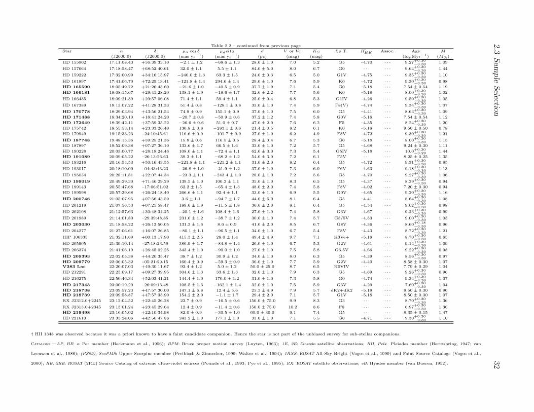
2.3Sam
ple
Selection
32Table 2.2 – continued from previous page
Star α δ µα cos δ µdelta d V or VT KS Sp.T. R′HK
Assoc. Age M
(J2000.0) (J2000.0) (mas yr−1) (mas yr−1) (pc) (mag) (mag) (log Myr−1) (M)
HD 155902 17:11:08.43 +56:39:33.10 −2.1 ± 1.2 −68.6 ± 1.3 28.0 ± 1.0 7.0 5.2 G5 –4.70 · · · 9.27+0.30
−0.301.09
HD 157664 17:18:58.47 +68:52:40.61 32.0 ± 1.1 5.5 ± 1.1 84.0 ± 5.0 8.0 6.7 G0 · · · · · · 9.64+0.30
−0.301.44
HD 159222 17:32:00.99 +34:16:15.97 −240.0 ± 1.3 63.3 ± 1.5 24.0 ± 0.3 6.5 5.0 G1V –4.75 · · · 9.35+0.30
−0.301.10
HD 161897 17:41:06.70 +72:25:13.41 −121.8 ± 1.4 294.6 ± 1.4 29.0 ± 1.0 7.6 5.9 K0 –4.72 · · · 9.30+0.30
−0.300.98
HD 165590 18:05:49.72 +21:26:45.60 −21.6 ± 1.0 −40.5 ± 0.9 37.7 ± 1.9 7.1 5.4 G0 –5.18 · · · 7.54 ± 0.54 1.19
HD 166181 18:08:15.67 +29:41:28.20 138.1 ± 1.9 −18.6 ± 1.7 32.6 ± 2.2 7.7 5.6 K0 –5.18 · · · 8.00+0.30
−0.301.02
HD 166435 18:09:21.39 +29:57:06.08 71.4 ± 1.1 59.4 ± 1.1 25.0 ± 0.4 6.8 5.3 G1IV –4.26 · · · 9.50+0.30
−0.301.05
HD 167389 18:13:07.22 +41:28:31.33 51.4 ± 0.8 −128.1 ± 0.8 33.0 ± 1.0 7.4 5.9 F8(V) –4.74 · · · 9.34+0.30
−0.301.07
HD 170778 18:29:03.94 +43:56:21.54 74.9 ± 0.9 155.1 ± 0.9 37.0 ± 1.0 7.5 6.0 G5 –4.41 · · · 8.63+0.30
−0.301.09
HD 171488 18:34:20.10 +18:41:24.20 −20.7 ± 0.8 −50.9 ± 0.6 37.2 ± 1.2 7.4 5.8 G0V –5.18 · · · 7.54 ± 0.54 1.12
HD 172649 18:39:42.11 +37:59:35.22 −26.6 ± 0.6 51.0 ± 0.7 47.0 ± 2.0 7.6 6.2 F5 –4.35 · · · 8.24+0.30
−0.301.20
HD 175742 18:55:53.14 +23:33:26.40 130.8 ± 0.8 −283.1 ± 0.6 21.4 ± 0.5 8.2 6.1 K0 –5.18 · · · 9.50 ± 0.50 0.78
HD 179949 19:15:33.23 –24:10:45.61 116.6 ± 0.9 −101.7 ± 0.9 27.0 ± 1.0 6.2 4.9 F8V –4.72 · · · 9.30+0.30
−0.301.21
HD 187748 19:48:15.36 +59:25:21.36 15.8 ± 0.6 116.5 ± 0.5 28.4 ± 0.4 6.7 5.3 G0 –5.18 · · · 8.00+0.30
−0.301.15
HD 187897 19:52:09.38 +07:27:36.10 133.6 ± 1.7 66.5 ± 1.6 33.0 ± 1.0 7.2 5.7 G5 –4.68 · · · 9.24 ± 0.30 1.11
HD 190228 20:03:00.77 +28:18:24.46 108.0 ± 1.1 −72.4 ± 1.1 62.0 ± 3.0 7.3 5.4 G5IV –5.18 · · · 10.0+0.30
−0.291.44
HD 191089 20:09:05.22 –26:13:26.63 39.3 ± 1.1 −68.2 ± 1.2 54.0 ± 3.0 7.2 6.1 F5V · · · · · · 8.25 ± 0.25 1.35
HD 193216 20:16:54.53 +50:16:43.55 −221.8 ± 1.1 −221.2 ± 1.1 31.0 ± 2.0 8.2 6.4 G5 –4.72 · · · 9.31+0.30
−0.300.85
HD 193017 20:18:10.00 –04:43:43.23 −26.8 ± 1.0 −21.9 ± 1.2 37.0 ± 1.0 7.3 6.0 F6V –4.63 · · · 9.18+0.30
−0.301.13
HD 195034 20:28:11.81 +22:07:44.34 −23.3 ± 1.1 −243.4 ± 1.0 28.0 ± 1.0 7.2 5.6 G5 –4.70 · · · 9.27+0.30
−0.301.06
HD 199019 20:49:29.30 +71:46:29.29 139.5 ± 1.0 100.3 ± 1.1 35.0 ± 1.0 8.3 6.5 G5 –4.37 · · · 8.39+0.30
−0.300.94
HD 199143 20:55:47.68 –17:06:51.02 62.2 ± 1.5 −65.4 ± 1.3 48.0 ± 2.0 7.4 5.8 F8V –4.02 · · · 7.20 ± 0.30 0.94
HD 199598 20:57:39.68 +26:24:18.40 266.6 ± 1.1 92.4 ± 1.1 33.0 ± 1.0 6.9 5.5 G0V –4.65 · · · 9.20+0.30
−0.301.16
HD 200746 21:05:07.95 +07:56:43.59 3.6 ± 1.1 −94.7 ± 1.7 44.0 ± 6.0 8.1 6.4 G5 –4.41 · · · 8.64+0.30
−0.301.08
HD 201219 21:07:56.53 +07:25:58.47 189.0 ± 1.9 −11.5 ± 1.8 36.0 ± 2.0 8.1 6.4 G5 –4.54 · · · 9.02+0.30
−0.300.98
HD 202108 21:12:57.63 +30:48:34.25 −20.1 ± 1.6 108.4 ± 1.6 27.0 ± 1.0 7.4 5.8 G3V –4.67 · · · 9.23+0.30
−0.300.99
HD 201989 21:14:01.80 –29:39:48.85 231.6 ± 1.2 −38.7 ± 1.2 30.0 ± 1.0 7.4 5.7 G3/5V –4.53 · · · 9.00+0.30
−0.301.03
HD 203030 21:18:58.22 +26:13:50.05 131.3 ± 1.6 8.6 ± 0.9 41.0 ± 2.0 8.5 6.7 G8V –4.36 · · · 8.60+0.18
−0.300.96
HD 204277 21:27:06.61 +16:07:26.85 −80.1 ± 1.1 −96.5 ± 1.1 34.0 ± 1.0 6.7 5.4 F8V –4.43 · · · 8.72+0.30
−0.301.21
HIP 106335 21:32:11.69 +00:13:17.90 415.3 ± 2.5 28.0 ± 1.4 49.4 ± 4.9 9.7 7.1 K3Ve+ –5.18 · · · 8.70+0.30
−0.300.85
HD 205905 21:39:10.14 –27:18:23.59 386.9 ± 1.7 −84.8 ± 1.4 26.0 ± 1.0 6.7 5.3 G2V –4.61 · · · 9.14+0.30
−0.301.09
HD 206374 21:41:06.19 +26:45:02.25 343.4 ± 1.0 −90.0 ± 1.0 27.0 ± 1.0 7.5 5.8 G6.5V –4.66 · · · 9.22+0.30
−0.300.98
HD 209393 22:02:05.38 +44:20:35.47 38.7 ± 1.2 30.9 ± 1.2 34.0 ± 1.0 8.0 6.3 G5 –4.39 · · · 8.56+0.30
−0.300.97
HD 209779 22:06:05.32 –05:21:29.15 160.4 ± 0.9 −59.3 ± 0.9 36.0 ± 1.0 7.7 5.9 G2V –4.40 · · · 8.58 ± 0.30 1.07V383 Lac 22:20:07.03 +49:30:11.67 93.4 ± 1.2 5.0 ± 1.2 50.0 ± 25.0 8.7 6.5 K0VIV · · · · · · 7.79 ± 0.29 1.04
HD 212291 22:23:09.17 +09:27:39.95 304.6 ± 1.3 33.6 ± 1.3 32.0 ± 1.0 7.9 6.3 G5 –4.69 · · · 9.26+0.30
−0.300.96
HD 216275 22:50:46.34 +52:03:41.21 144.4 ± 1.0 170.0 ± 1.2 31.0 ± 1.0 7.3 5.8 G0 –4.74 · · · 9.34+0.30
−0.301.07
HD 217343 23:00:19.29 –26:09:13.48 108.5 ± 1.3 −162.1 ± 1.4 32.0 ± 1.0 7.5 5.9 G3V –4.29 · · · 7.60+0.30
−0.301.04
HD 218738 23:09:57.23 +47:57:30.00 147.1 ± 6.8 12.4 ± 5.6 25.3 ± 4.9 7.9 5.7 dK2+dK2 –5.18 · · · 8.50 ± 0.30 0.90HD 218739 23:09:58.87 +47:57:33.90 154.2 ± 2.0 −1.1 ± 1.7 29.4 ± 2.0 7.1 5.7 G1V –5.18 · · · 8.50 ± 0.30 1.07
RX J2312.0+2245 23:12:04.52 +22:45:26.28 23.7 ± 0.9 −16.5 ± 0.6 150.0 ± 75.0 9.9 8.3 G3 · · · · · · 8.70+0.30
−0.301.36
RX J2313.0+2345 23:13:01.24 +23:45:29.64 12.4 ± 0.9 −11.4 ± 0.6 150.0 ± 75.0 10.2 8.6 F8 · · · · · · 6.97+0.30
−0.301.36
HD 219498 23:16:05.02 +22:10:34.98 82.0 ± 0.9 −30.5 ± 1.0 60.0 ± 30.0 9.1 7.4 G5 · · · · · · 8.35 ± 0.15 1.47
HD 221613 23:33:24.06 +42:50:47.88 243.2 ± 1.0 177.1 ± 1.0 33.0 ± 1.0 7.1 5.5 G0 –4.71 · · · 9.30+0.30
−0.301.10
† HII 1348 was observed because it was a priori known to have a faint candidate companion. Hence the star is not part of the unbiased survey for sub-stellar companions.
Catalogs.—AP, HE: α Per member (Heckmann et al., 1956); BPM: Bruce proper motion survey (Luyten, 1963); 1E, 2E: Einstein satellite observations; HII, Pels: Pleiades member (Hertzspring, 1947; van
Leeuwen et al., 1986); (PZ99), ScoPMS: Upper Scorpius member (Preibisch & Zinnecker, 1999; Walter et al., 1994); 1RXS: ROSAT All-Sky Bright (Voges et al., 1999) and Faint Source Catalogs (Voges et al.,
2000); RE, 2RE: ROSAT (2RE) Source Catalog of extreme ultra-violet sources (Pounds et al., 1993; Pye et al., 1995); RX: ROSAT satellite observations; vB: Hyades member (van Bueren, 1952).

2.4 Sample Biases and Discussion 33
2.4 Sample Biases and Discussion
Some of the sample selection criteria outlined in the previous section introduce obvious biasesmostly against, and less often in favor of, miltiplicity in the survey. These are discussed below.
2.4.1 Examining the Biases
First of all, criteria (1–3), (11–12), and (14) do not introduce any multiplicity biases. Theremainder may do so to varying extents.
Criterion (4): The requirement for good quality 2MASS photometry with no flags mayexclude stars in binary pairs with separations of several arcseconds, as these could contaminateeach other’s photometry. However, because of criterion (5), such resolved (or de-blended)companions should not be present in the sample in the first place. Therefore, criterion (4) doesnot introduce bias beyond that already introduced by criterion (5).
Criterion (5): This requirement introduces an obvious bias against close stellar binary pairs.Given the range of heliocentric distances of stars in the sample, and assuming that 2.0′′ (≈2times the size of the 2MASS resolution element) is the minimum angular separation at whichpoint sources in 2MASS can be resolved, companions in the 20–1000 AU projected separationrange may be excluded. In practice, because of the limited dynamic range of 2MASS observa-tions within 5′′ of bright stars (∼4.5 mag at 5′′, ∼2.5 mag at 3′′; cf. Fig. 11 in Cutri et al., 2003),this criterion excludes mostly near-equal magnitude stellar companions. Sub-stellar compan-ions will be too faint to be detected in such close proximity to bright stars in 2MASS, even atthe youngest ages and even around the coolest (K5) stars in our sample.
Criterion (6): On one hand, similarly to the previous criterion, this selection criterion willexclude mostly equal-flux binaries, though over a wider range of projected physical separations(20–2500 AU). On the other hand, the criterion also excludes stars with projected faint redcompanions–potential brown dwarfs. However, because the criterion is applied only to stars100 Myr and older, and because of the limited dynamic range of the 2MASS Point SourceCatalog within 12.8′′ (. 6 mag), this criterion introduces a bias against sub-stellar companionsin only a limited number of cases. The systems that may be excluded are late-type (K0–K5) dwarf primaries with massive (60–72MJup) sub-stellar companions. These are expected tocontribute a small fraction (<10%) of the existing solar analog/brown dwarf pairs and thusshould not have a dramatic effect on the overall result.
Criterion (7): Given the unknown multiplicity selection criteria for these GTO programs,and the small number of discarded stars, the effect is likely unimportant. It is possible that thestars removed from the target list as a result of this criterion may be preferentially single.
Criterion (8): This criterion biases the sample against nearly equal-flux or equal-mass binarystars, with separations between 0 AU and 400 AU.
Criterion (9): Given that current observational evidence of the effect of stellar multiplicityon disk frequency does not support a correlation between the two phenomena (e.g., Bouvieret al., 1997), the effect of the addition of stars with known IR excesses on multiplicity is likelyneutral. Indeed, one of the IR-excess stars added in this process, HD 134319, is a known triplesystem (Lowrance et al., 2005).
Criterion (10): Given that there is no clear evidence that extra-solar planets cannot existin wide (&10 AU) multiple systems, the addition of the few exo-planet host stars to the sampleis not expected to affect the statistics of stellar and sub-stellar companions detectable in direct

2.5 Unique Advantages of the Present Survey in Comparison to Others 34
imaging.Criterion (13): The application of this requirement hinders the discovery of faint companions
in nearly equal-flux binary systems to the extent that such binaries were not removed alreadyby criteria (5) and (6). It is therefore a bias against higher-order multiples. It does not biasagainst the detection of faint secondary companions to single stars.
Criterion (15): When open cluster stars were added to the deep sample, that was donein an unbiased manner, without regard for the existence of previous high angular resolutionobservations.
2.4.2 Discussion
The complete set of target selection requirements outlined in §2.2.1–§2.2.3 and the subsequentexclusion criteria (1–14) are largely unbiased toward the detection of sub-stellar companionsaround most Sun-like stars, with the exception of 60–75MJup brown dwarfs in orbit aroundK0–5 V stars and brown dwarfs orbiting near equal-flux (∆KS < 4 mag) binaries. As alreadypointed out, the exclusion of the star/brown-dwarf combinations in the first case is not expectedto have a large effect on the estimated brown-dwarf companion frequency. The bias has beenignored in the discussion of the survey incompleteness in §6. Similarly, the exclusion of binarysystems from the deep sample will leave the analysis of the sub-stellar companion frequencyaround single stars unaffected.
The binary exclusion criteria will, on the other hand, strongly influence the observed stellarmultiplicity, biasing the survey toward discovering a smaller fraction of binaries and multiples.Because of the complicated nature of the biases, an attempt to correct for them has not beenmade. Only a cursory discussion of stellar multiplicity is provided in §6.
2.5 Unique Advantages of the Present Survey in Com-
parison to Others
The distinctive features of the Palomar/Keck AO companion survey are: (1) its emphasis onyoung stars, (2) its focus on solar analogs, and (3) its use of high-order AO systems. We discussthe uniqueness and advantages of these characteristics in the following sections.
2.5.1 The Palomar/Keck AO Sample is Young
With a median age of 80 Myr and 101 stars in the deep imaging sample, the present surveytargets the youngest and most comprehensive sample of young stars that has been scrutinizedfor sub-stellar companions. In comparison, previous high-contrast imaging surveys of similarsize (>50 stars: Oppenheimer et al., 2001; Close et al., 2003; Beuzit et al., 2004; McCarthy &Zuckerman, 2004; Carson et al., 2005) have concentrated on nearby and typically older stars.Because of the lack of star-forming regions within 100 pc of the Sun, such surveys are dominatedby stars with ages similar to that of the Sun (4.56 Gyr). The several dozen known members ofyoung (10–35 Myr) kinematic groups within 100 pc from the Sun–Tucana/Horologium (Zucker-man & Webb, 2000; Torres et al., 2000), TW Hydra (Kastner et al., 1997; Torres et al., 2000),and β Pictoris (Zuckerman et al., 2001a))–have already been targeted, often repeatedly, bysmaller high-contrast surveys (Chauvin et al., 2003; Neuhauser et al., 2003; Masciadri et al.,
2.5 Unique Advantages of the Present Survey in Comparison to Others 35
2005; Lowrance et al., 2005). The limited number of known members of these groups, .40altogether, precludes statistically significant conclusions. A notable exception to this trend isthe work of McCarthy & Zuckerman (2004), which boasts the exploration of 178 stellar systemswith a median age of 300 Myr, 90% of which lie within 25 pc of the Sun. However, a closer ex-amination of this work reveals that the mean sample age has probably been under-estimated bya factor of ∼3. Hence, the sensitivity of the McCarthy & Zuckerman survey to sub-stellar com-panions is significantly poorer than claimed. This survey is given a more detailed considerationin §7.
Given the rapid decline in intrinsic luminosity of objects below the hydrogen-burning limitwith age, surveys of solar neighborhood stars are often less sensitive to objects of sub-stellarmass than surveys concentrating on more distant, significantly younger stars. For example, a0.05M brown dwarf is expected to decrease in brightness by 6.7 mag in the K band betweenthe ages of 100 Myr and 5.0 Gyr (Baraffe et al., 2003). Lower-mass objects are expected tocool even faster: over the same period, a 0.01M object dims by 15.8 mag at K! Providedthat such young stars can be identified, allowing a corresponding increase (by a factor of 22 to1400) in the mean heliocentric distance of the survey targets is justified, if sensitivity to lowmasses is the primary goal. Since a number of 1–100 Myr-old associations of young stars existwithin 200 pc (distance modulus of 6.5 mag), imaging observations of them will likely producebrown dwarfs of much lower mass than any of the 1–10 Gyr-old brown dwrafs discovered in thesolar neighborhood. Indeed, several brown dwarfs with estimated masses near and below thedeuterium-burning limit (∼ 13MJup; Burrows et al., 1997) have been reported in the nearest(50–160 pc) associations of 1–15 Myr-old stars, both in isolation (e.g., Lucas et al., 2001; Bricenoet al., 2002) and, more recently, as companions to more massive objects (Chauvin et al., 2004,2005b; Neuhauser et al., 2005).
Naturally, the ability to resolve such brown dwarfs and candidate giant planets in the vicinityof host stars decreases linearly with increasing heliocentric distance. Direct imaging surveysfor companions to more distant young stars will be sensitive only to objects in correspondinglywider orbits. Therefore, while proximity to ths Sun was of secondary importance, after youth,in constructing the deep sample, among stars of the same age, the nearer ones were givenpreference whenever possible.
Figure 2.5 displays the complete (open circles) and the deep (filled circles) samples on anage vs. distance diagram. The horizontal dashed line in the Figure delimits the maximum ageof stars included in the deep sample. Given the age vs. distance selection for stars in the deepsample, the final survey is most sensitive to 12–72 MJup companions at projected separationsbetween approximately 20 and 1200 AU (§6.2.3).
2.5.2 The Palomar/Keck AO Sample Has a High Median Mass
The median primary spectral type for the Palomar/Keck survey is G5, which at the 80 Myrmedian sample age is equivalent to a mass of ≈ 1.0M (Baraffe et al., 1998). The survey isfocussed on solar-type stars in order to establish the low-mass multiplicity characteristics ofstars similar to the Sun. On the other hand, sub-stellar companion surveys focussing on nearbystars are dominated by late K and M stars, as expected from volume-limited stellar samples.As a result, the mean primary mass in those surveys is smaller, ∼ 0.5M (spectral type M0 V).Thus, the Palomar/Keck survey explores a distinct population of stars that is on average afactor of 2 more massive than that surveyed for sub-stellar companions previously.

2.5 Unique Advantages of the Present Survey in Comparison to Others 36
Figure 2.5: Age vs. heliocentric distance diagram for the complete survey sample (open circles)and for the deep sub-sample (filled circles). The errorbars at the bottom left denote the meanerrors in age and distance. The horizontal dashed line delimits the maximum age for starsincluded in the deep sample.
2.5 Unique Advantages of the Present Survey in Comparison to Others 37
The advantages of targeting more massive stars may not be immediately obvious. Moremassive stars are more luminous and hence require higher imaging contrast to achieve sensitivityto companions of sub-stellar masses. Several surveys have in fact deliberately focused on faintprimaries, such as white dwarfs (Zuckerman & Becklin, 1992; Farihi et al., 2005), M dwarfs(Beuzit et al., 2004), and ultra-cool dwarfs (later than M7; Martin et al., 1999; Reid et al., 2001;Close et al., 2003; Burgasser et al., 2003; Bouy et al., 2003), as a way to reduce the need forhigh contrast in resolving faint close-in objects. These surveys do indeed probe for companionmasses well below the hydrogen-burning limit. The resulting picture is that brown dwarfs andlow-mass stars reside primarily in tight (< 15 AU) nearly equal-mass (q ≥ 0.7) systems (Closeet al., 2003). Examples to the contrary, as recently presented in Chauvin et al. (2005a) andLuhman (2004), are still considered exceptions. The most direct explanation for this is that low-mass multiples inhabit shallower potential wells and are therefore easily disrupted as a result ofthe frequent stellar encounters typical of star-forming regions. Hence, low-mass binaries in tightorbits survive preferentially. Conversely, higher-mass stars can maintain gravitationally boundcompanions at larger orbital semi-major axes, which can survive dynamical perturbations bypassing stars.
The first advantage of looking for sub-stellar companions around more massive stars isthat the companions can be expected to exist at wider separations. Indeed, all of the directlyimaged brown dwarf companions to & 0.3M stars (i.e., excluding the ultra-cool binaries) resideat projected separations between 14 AU and 3600 AU. This is a particularly important featureof companions to more massive systems in the context of the Palomar/Keck young stars surveybecause of the greater median heliocentric distance of the sample. That is, by concentratingthe Palomar/Keck effort on more massive and younger (and by necessity, more distant) stars,we can hope to resolve some of the least massive sub-stellar companions to solar-type stars.The detection limits of the survey are such that this allows us to probe, albeit only partially(§6.2.3) for objects with masses below the deuterium burning limit–potential extrasolar giantplanets.
The second advantage of having a relatively massive sample of stars is that, absolute massestimates aside, the sub-stellar secondaries in systems are more prominent at a fixed mass ratioq. For example, a 500 Myr-old 1M star orbited by a 0.05M brown dwarf (q = 0.05) hasan expected K-band flux ratio of 7.8 mag (Baraffe et al., 1998, 2003). On the other hand, a0.6M + 0.03M system (also q = 0.05) at the same age has a projected K-band flux ratio of8.5 mag and thus requires higher contrast for detection. The effect is more pronounced at evenlower mass ratios. Hence, high-contrast imaging surveys of appropriately selected samples ofyoung massive stars allow the opportunity to study the dynamical survival of low mass ratio(q < 0.1) systems with unprecedented sensitivity and statistics. This fact is exemplified byrecent AO surveys of B (Shatsky & Tokovinin, 2002) and A (Kouwenhoven et al., 2005) starsin the 5–20 Myr-old Scorpius OB2 association (de Zeeuw et al., 1999; Mamajek et al., 2002).With only minor (0–25%) corrections for incompleteness, the authors of the two surveys findthat & 20% of all multiple systems with B and A primaries have mass ratios q ≤ 0.1. The resultis not unexpected in view of radial-velocity and direct imaging multiplicity surveys of lower-mass FGK dwarfs (e.g., Duquennoy & Mayor, 1991; Mazeh et al., 2003; Patience et al., 2002).However, the latter are severely (80–100%) incomplete at these low mass ratios. Hence, thecombination of a relatively massive sample of young stars and high-contrast imaging allows theopportunity to explore low-mass ratio systems to a high level of completeness. A high-contrastsurvey of the multiplicity of young solar analogs similar to those of young B and A stars has
2.5 Unique Advantages of the Present Survey in Comparison to Others 38
not been performed. The present survey fills this gap.
2.5.3 The Palomar/Keck Survey Uses a High-Order AO System
The PALAO system (Troy et al., 2000) employs a 349-element deformable mirror (DM) behinda Shack-Hartmann wavefront sensor. A similar DM is used in the Keck AO system (Wiz-inowich et al., 2000). They are considered high-order AO systems as they are able to correct alarger number of modes in the Zernicke polynomial expansion of the incoming wavefront than“curvature” AO systems, which employ deformable mirrors with smaller numbers (20–50) ofactive elements. In broad terms, the result is improved dynamic range in the vicinity of bright(R . 10 mag) stars though compromised performance at the faint (R & 12 mag) end. Giventhat the survey targets are all brighter than R = 12, the PALAO and Keck AO systems areoptimally suited for this study.
The majority of the large ground-based surveys discussed above have either not used AO(McCarthy & Zuckerman, 2004) or used only low-order tip-tilt or curvature AO (Oppenheimeret al., 2001; Close et al., 2003; Beuzit et al., 2004). They thus suffer from 2–5 mag poorer con-trast in the vicinity of bright stars, compared to the present Palomar/Keck survey, effectivelypreventing the discovery of close-in sub-stellar companions. Recent exceptions to this rule arethe Carson et al. (2005) survey of old solar neighborhood stars, which also used PALAO, butfocused on older stars and thus lacks comparable companion sensitivity, and the VLT/NACO(Masciadri et al., 2005) and HST/NICMOS (Lowrance et al., 2005) surveys, which reach ap-proximately 1 mag deeper.
2.5.4 Comparison to Recent, Higher-Contrast Surveys and Sum-mary
Since the Palomar/Keck AO survey began in 2002, the complete results from one medium-sized(45 stars; Lowrance et al., 2005) and one small (28 stars; Masciadri et al., 2005) high-contrastsurveys have been announced. In addition, discoveries of sub-stellar companions from twoother such surveys in progress have been published (Chauvin et al., 2005a,b; Neuhauser et al.,2005). The rate of detection of sub-stellar companions from these has been markedly higher incomparison to previous surveys, with a total of 5 discovered.
All of these surveys have attained ∼1 mag higher contrast than the present Palomar/Kecksurvey, by virtue of their use of HST/NICMOS (Lowrance et al.) or of the novel high-order AOsystem NAOS (Rousset et al., 2000) on the VLT (Masciadri et al.; Chauvin et al.; Neuhauseret al.). Most of these, with the exception of the HST survey, focus on southern stars (δ <−30), inaccessible from Palomar. Partially as a result of this, all 5 of the bona fide sub-stellar companions reported in these surveys orbit stars with declinations δ < −30. Thereason for this north-south asymmetry in survey focus and success rate, in addition to theconcentration of technology at the southern latitude of the VLT, is the larger concentrationof known nearby young stellar moving groups in the southern hemisphere. Consequently, thenorthern hemisphere remains relatively unexplored for sub-stellar companions to young stars.The Palomar/Keck AO survey fills this niche by taking advantage of the recent vast compilationof young solar analogs over the entire sky, made available to us through the FEPS team.
Therefore, the Palomar AO survey of young solar analogs presented here is unique in itsscale, sensitivity, and focus on young stars at northern declinations.

Chapter 3
Observations and Methodology
3.1 Overview
This Chapter presents two examples of the observational and analytical steps that we followedin: (1) searching for low-mass companions to young stars, (2) confirming their physical associ-ation with the respective stars, and (3) establishing their mass.
Section §3.2 presents a pilot study for sub-stellar companions to the nearby (7.8 pc) ∼300 Myr-old (Barrado y Navascues, 1998; Song et al., 2001) star α Lyr (Vega) conducted at the beginningof the observing campaign. Because of its early spectral type (A0), Vega was not included inthe solar analog survey. The study, published in Metchev et al. (2003), is included here as an in-troduction to the near-IR high-contrast imaging possibilities with the Palomar AO system andas a demonstration that planetary-mass companions to nearby stars are potentially detectablein direct imaging with ground-based telescopes.
Section §3.2 also presents the principal approach that we have employed for deciding thephysical association between a star and a candidate companion: establishing common propermotion through differential astrometry. Although a gravitational bond between two celestialbodies can be claimed unambiguously only after solving for a common orbit, for resolved stel-lar systems this typically requires multiple observations over many years. In the meantime,however, the common space motion of a nearby binary system sets it apart from backgroundstars, which, because of their much higher heliocentric distances, appear stationary. Therefore,by establishing common space motion between a pair of high-proper-motion stellar or sub-stellar objects with respect to background objects, one can infer that the pair is gravitationallybound. This requires only two observations taken over a period of time generally much shorterthan the orbital period. The required time-span is inversely proportional both to the apparentproper motion of the stars and to the precision of the astrometric measurements. In the caseof Vega, owing to the high proper motion of the star (351 mas yr−1; Perryman et al., 1997),adequate astrometric follow-up with PALAO was possible within two months of the first-epochobservations. For the smaller apparent proper motions of the stars in the companion survey(.100 mas yr−1), time-spans of 1–3 years and a more accurate astrometric calibration of thePHARO pixel scale (§4) were required.
Section §3.3, published in Metchev & Hillenbrand (2004), contains a detailed description ofthe observing strategy (§3.3.2) in seeking and confirming candidate companions to solar analogswith the Palomar and Keck AO systems. It also presents the three principal approaches that wehave used to estimate companion masses: (i) near-IR colors and absolute magnitudes (§3.3.3.1),
39

3.1 Overview 40
(ii) near-IR spectroscopy (§3.3.3.3), and (iii) orbital motion (§3.3.4.3.1). These are applied tothe newly-discovered and confirmed companions to stars in the survey: a sub-stellar companionto HD 49197 and stellar companions to HD 129333, V522 Per, and RX J0329.1+0118. Meth-ods (i) and (ii) rely on empirical relations to estimate the luminosities and temperatures of thecompanions (assuming the same distance and age as those of the respective primary), which arethen compared to theoretical predictions for cool and ultra-cool dwarfs. The third approach,applied only to the HD 129333A/B system, demonstrates the power of combining high angularresolution imaging and radial velocity monitoring in solving for dynamical masses in binarysystems. Finally, we show that in cases of candidate binary systems where physical associationmay not be conclusively decided through relative astrometry, statistical arguments, based on acomparison between the spectroscopically-determined temperature and luminosity of the com-panion and the known space density of similar objects, offer a powerful tool in constraining thelikelihood for physical association (§3.3.4.1).

3.2 Adaptive Optics Observations of Vega 41
3.2 Adaptive Optics Observations of Vega
†Stanimir A. Metchev, Lynne A. Hillenbrand, & Russel J. White
California Institute of Technology, Division of Physics, Mathematics & Astronomy, MC 105–24, Pasadena,California 91125
Abstract
From adaptive optics observations with the Palomar 5-meter telescope we place upper limits onthe masses of any planetary companions located between ∼30–230 AU away from Vega, whereour data are sensitive to depths ranging from H = 12.5 mag to H = 19.0 mag fainter thanVega itself. Our observations cover a plus-shaped area with two 25′′ × 57′′ elements, excluding7′′ × 7′′ centered on the star. We have identified 2 double and 4 single point sources. Theseprojected companions are 14.9–18.9 mag fainter than Vega and if physically associated wouldhave masses ranging from 4 to 35 MJup and orbital radii 170–260 AU. Recent simulations ofdusty rings around Vega predict the presence of a perturbing body with mass <2–3 MJup andorbital radius ∼40–100 AU, though more massive (.10 MJup) planets cannot be excluded. Noneof the detected objects are this predicted planet. Based on a color-magnitude, spectroscopic,and proper motion analysis, all objects are consistent with being background sources. Giventhe glare of Vega, a 2 MJup object near the expected orbital radii would not have been visible atthe 5σ level in our data, though any >10 MJup brown dwarf could have been seen at separation>80 AU.
3.2.1 Introduction
The A0V star Vega is famously known since the early days of data return from IRAS as a youngmain sequence star surrounded by dust (Aumann et al., 1984). Its age (270–380 Myr; Song et al.,2001) combined with the large fractional excess luminosity at infrared wavelengths (Lexcess/L∗ ≈10−5 or Mdust ≈ 1/2Mmoon; Backman & Paresce, 1993) imply that dust is being generated atthe current epoch by either grinding collisions between larger rocky bodies, a.k.a. planetesimals(Harper et al., 1984; Weissman, 1984; Zuckerman & Becklin, 1993), or in cometary ejecta(Beust et al., 1989, 1990, and references therein). If the dust is not continuously regeneratedit will be depleted by a combination of Poynting-Robertson drag and radiation pressure on atime-scale much shorter than the age of Vega. Discovery of the infrared excess around Vegaand other main sequence stars too old to possess the so-called primordial dust and gas disksthat are commonly found around 1–10 Myr-old stars, led to coining of the term “debris disk.”Searches for other examples of “the Vega phenomenon” have led to the cataloging of a meretens of objects (see, e.g., Mannings & Barlow, 1998; Silverstone, 2000), mostly early-type starswhose dust was detectable with IRAS or ISO, or observable from the ground with mid-infraredinstrumentation on large telescopes.
The mid- and far-infrared (25–850 µm) emission from Vega is extended over tens of arcsec-onds (Aumann et al., 1984; Harvey et al., 1984; Zuckerman & Becklin, 1993; Heinrichsen et al.,1998; Holland et al., 1998). Aperture synthesis imaging at 1.3 mm (Koerner et al., 2001; Wilner
†A version of this Section was published in The Astrophysical Journal, vol. 582, 1102

3.2 Adaptive Optics Observations of Vega 42
et al., 2002) resolved several dust clumps located ∼8–14′′ from the central source (60–110 AU,assuming the Hipparcos parallax of 128.9 milli-arcsec). One interpretation is that these clumpstrace the densest portions of the already inferred face-on circumstellar ring (Dent et al., 2000).Additional support for a ring interpretation comes from Vega’s spectral energy distribution,which is close to photospheric at shorter wavelengths (.20 µm; Heinrichsen et al., 1998), andsuggests an inner gap in the density distribution that may or may not be entirely devoid of hotdust. At 11.6 µm extensions larger than 1/4′′ are ruled out by the imaging of Kuchner et al.(1998). Interferometric work by Ciardi et al. (2001), however, did suggest extended emissionat 2.2 µm.
Observations of structure in the circumstellar dust around Vega have spawned detailedmodels for a planetary perturber (Gorkavyi & Taidakova, 2001; Wilner et al., 2002). Resonancetrapping and gravitational scattering induced by a body of mass 2–3 MJup are consistent withthe Holland et al. (1998) map and with the interferometric observations of Koerner et al. (2001)and Wilner et al. (2002). Due to degeneracies in dynamical models (e.g., Wilner et al., 2002),more massive planets (∼10 MJup) also cannot be ruled out. Modeling to date assumes a face-onorientation of the presumed dust disk or ring. Evidence for this geometry comes both from aring-shaped (e.g., Heinrichsen et al., 1998) albeit clumpy (Koerner et al., 2001; Wilner et al.,2002) dust distribution and from detailed analysis of stellar line profiles (assuming parallel diskand stellar rotation axes; Gulliver, Hill, & Adelman, 1994).
Our experiment was designed to search for low-mass companions within 4–30′′ of Vega, inpart to test the aforementioned planetary perturber predictions. Imaging observations close tothis bright source are usually “burned out” in survey data such as POSS or 2MASS. Ground-based coronagraphic observations (Smith et al., 1992; Kalas & Jewitt, 1996) have also lackedsufficient sensitivity. Except for NICMOS images (Silverstone et al., 2002) with sensitivitycomparable to ours, high dynamic-range observations have not been previously reported.
3.2.2 Observations
Data were obtained with the Palomar adaptive optics (PALAO; Troy et al., 2000; Bloemhofet al., 2000) system in residence at the Palomar 5-m telescope. PALAO employs PHARO,the Palomar High Angular Resolution Observer (Hayward et al., 2001), a 10242 pix HgCdTeHAWAII detector with imaging (25′′ or 40′′ field of view) and spectroscopic (R =1500–2500)capabilities. Broad- and narrow-band filters throughout the JHK atmospheric windows areavailable, as well as a choice of coronagraphic spot sizes and Lyot masks.
Vega was observed on the night of 2002 June 22 with additional follow-up observationsobtained on August 28 and 29 (UT), all under photometric sky conditions. The observingstrategy was to take deep images in H-band to maximize the detection likelihood of faint low-mass objects (see e.g., Burrows et al., 1997). The point spread function (PSF) was 0.6–0.9′′
uncorrected at H-band and improved to <0.1′′ with adaptive correction. A neutral densityfilter (1%) manually placed in front of the wave front sensor (WFS) enabled AO lock on such abright object. AO performance was very good during most of the observing, with Strehl ratiosup to 20% in H . We did not employ the coronagraphic mode of PALAO for these observationssince scattered light suppression was not sufficient enough to prevent saturation on the arrayoutside the boundaries of the largest coronagraph (0.97′′ = 12λ/D in H) in the shortest possibleintegration time (1897 milli-sec).
On June 22, a total of 26 minutes on-source integration was obtained with the 25′′ field of

3.2 Adaptive Optics Observations of Vega 43
view in H-band at each of 4 pointings: north, south, east, and west around Vega (henceforth:Vega N, S, E, and W fields), with Vega itself located 3.5′′ off of the imaging field at eachpositioning of the telescope. Due to field overlaps, ∼13% of the area covered (2210 arcsec2)was observed for 52 minutes. Dithering at the 0.25–1.00′′ level was performed for the on-source frames. More widely dithered sky frames were taken at locations ∼2′ farther awayfrom Vega with source-to-sky time split 2:1. The integration time for individual exposureswas 10.9 seconds. For the eastern field in which several objects were noticed in real time, wealso obtained J , H , and Ks data with 2.5 minutes total on-source integration time taken as 5separate frames, with Vega offset 22–28′′ to the west. The airmass range was 1.03–1.30 for theentire observing sequence.
Photometric calibration was achieved via immediate observation of 2MASS 183726.28 +385210.1 (GSC 03105–00679, a G8V star) located ∼7.7′ from Vega with 2MASS magnitudesKs = 8.296 ± 0.033, H = 8.365 ± 0.022, and J = 8.745 ± 0.028. This source, although not aphotometric standard, is sufficient as a local calibrator and was observed at airmass 1.35. Twoother much fainter 2MASS sources are also present in the image.
During the second epoch observations, resolution R = 1500 and 2400 K-band spectra ofthe brightest discovered object were obtained (August 28) through a 0.52′′ slit and a K grismfor a total of 100 minutes on-source integration. The object was dithered 10′′ along the slit forsky-subtraction. Spectra of scattered light from Vega were used as a telluric standard. Short-exposure (5 minutes per filter) dithered JHKs images were taken (August 29) as follow-up tothe June 22 data to test for common proper motion with Vega. The airmass of Vega for thesecond epoch observations varied between 1.01 and 1.13.
We also observed a binary system (HD 165341) with a well-determined orbit in the SixthCatalog of Orbits of Visual Binary Stars1 in order to determine precisely the plate-scale andorientation of the PALAO system. We derive for the 25′′ field a plate-scale of 0.025168 ±0.000034 arcsec/pixel.
3.2.3 Data Processing
Our image reduction steps, written in IDL and IRAF, include the standard procedures of flat-fielding, sky-subtracting, interpolating/masking bad pixels, and mosaicking the dither pattern.This last step required correcting for image drift (likely caused by change in the direction ofthe gravity vector in PHARO over the duration of the observing sequence), the rate of whichvaried between 0.5 and 1.2 arcsec/hour.
Image stacks from each of the four deep pointings (June 22) were registered to the firstimage in the series. For the east field in which several point sources were detected, each imagewas registered by centroiding on the brightest object. For the north field, centroiding waspossible on the bright reflection artifact due to Vega. For the other two fields registration wasaccomplished by first averaging sets of 9 consecutive exposures, extrapolating the position ofVega from the intersection of 6 scattered light “rays” in the image halo, and combining the16 registered averages. In this manner, the location of the star could be constrained to within±5.0 pix = ±0.13′′ (c.f. ±0.10 pix for our mean centroiding precision in the north and east fields).We did attempt cross-correlation techniques for dither pattern correction but these were notas successful as the above procedures. The final step was to orient the images with north–upand east–left. Astrometric calibration was established assuming the plate-scale derived from
1Available at http://ad.usno.navy.mil/wds/orb6.html.

3.2 Adaptive Optics Observations of Vega 44
the binary star observations and by reference to the Hipparcos (J2000.0) coordinates of Vega.Our final image of the Vega vicinity is presented in Figure 3.1a.
Various methods to reduce the large halo from Vega were attempted, including reflections,rotations, and data smoothing. Shown in Figure 3.1b is a difference image, for which a Gaussian-smoothed (σ = 5 pix, FWHM = 12 pix; c.f. FWHM = 4 pix for the point sources) version of theoriginal image has been subtracted. This procedure effectively removes large scale gradients.Strong artifacts do remain, however, and contribute to our limited sensitivity to point sourceswithin ∼10′′ of Vega.
Spectra of the brightest point source were extracted using the APALL task within IRAF. Aquadratic polynomial was fit to all pixels with values >10% of the peak flux along an aperture.Local background was estimated from a region 0.50–1.25′′ from the aperture center. The ex-tracted spectra were divided by that of the telluric standard (with the 2.166 µm Brγ absorptionfeature interpolated over) to correct for instrumental response and atmospheric transmission.Wavelength calibration was done by fitting a dispersion relation to sky OH emission lines.Finally, the wavelength-calibrated spectra were co-added.

3.2A
dap
tiveO
ptics
Observation
sof
Vega
45
18:36:59.0 57.5 56.0 54.5
38d47m00s
50s
40s
10s
20s
30s
(a)
7,8
6
5,4
32
1
18:36:59.0 57.5 56.0 54.5
38d47m00s
50s
40s
10s
20s
30s
(b)
7,8
6
5,4
32
1
Figure 3.1: (a) Composite H-band mosaic of the Vega region obtained with PALAO. Eight point sources are detected, 5 to the east,2 to the south-east, and 1 to the north of Vega. The two close, eastern-most objects are just off the edge of the deep exposure of theVega E field, but have been pasted in from our shallower JHKs images, obtained for photometry purposes, to show their location.Similarly, the double source to the south-east was discovered only in the follow-up shallow JHKs observations. A bright “ghost”reflection of Vega is also visible in the north field. (b) The same image, with a smoothed (σ = 5 pix) version of itself subtracted,to enhance faint sources in the wings of Vega’s halo.

3.2 Adaptive Optics Observations of Vega 46
3.2.4 Photometry of Detected Sources
The positions of identified sources are indicated in Figure 3.1. During the first epoch of obser-vations we detected 6 point sources, 5 of which were to the east of Vega. Four of these are singlewhile two are a close (0.6′′) double, which is 0.7′′ off the east edge of our deep Vega E image,and were observed only in the short JHKs exposures. The sixth point source is in the northfield. During the follow-up observations we detected another double (0.8′′) source south-east ofVega. PSF fitting techniques suggest these are in fact all stellar point sources and not partiallyresolved galaxies.
We performed photometry using both aperture and PSF techniques. First, we used theIRAF/PHOT task in the short exposures with aperture radii of 10 (Ks), 18 (H), and 32 (J)pixels (0.50′′, 0.90′′, and 1.5′′ diameters on the sky) chosen to correspond to 2 × FWHM ofthe image core and to include the first Airy ring. The mode of the counts in a 30–40 pixelannulus provided local sky that was critical for subtracting residual scattered light from Vega.For sources 1–6, magnitudes in each of the bands were obtained by comparing the measuredaperture flux to that of the 2MASS standard in the same aperture. The magnitudes andpositions of sources 7 and 8 were boot-strapped from those of source 1, with its error addedin quadrature. Airmass corrections were applied using extinction coefficients for Palomar aspreviously determined by L.A.H. (0.114, 0.029, and 0.065 magnitudes per airmass in J , H , andK, respectively). We also used the PSF, PEAK, and ALLSTAR tasks in IRAF/DAOPHOTfor PSF fitting photometry. PSF fitting worked best at Ks-band but required a large numberof iterations at H and J for convergence in part because the stellar profiles are not diffractionlimited. Differences between the aperture and PSF-fitting magnitudes are 0.2–0.3 mag (muchlarger than the formal errors), and the scatter of the PSF magnitudes is 50% larger than thatof the aperture magnitudes at J and H .
Our photometry (Table 3.1) is from apertures, except for sources 4 and 5, for which wesimultaneously fit PSF profiles to each of the components of the double source to determine theirmagnitude difference. A larger aperture (2.5′′ diameter—to include the PSFs of both sourcesat all bands) is used to measure a combined flux, and individual magnitudes are obtained fromthe large-aperture magnitude and the magnitude difference from PSF fitting. The photometryfor these two sources is less precise due to a more uneven background.
Repeatability of the photometry from frame to frame was assessed using aperture photom-etry on the calibration field, which is free of the bright background present in the Vega fields.We find 0.04 mag r.m.s. scatter between the 5 frames. For the shallow JHKs exposures nearVega, frame-to-frame differences are larger due to background variations induced by ditheringthat placed Vega closer to the image area for some frames than for others. We have includedthis scatter in our errors.
We do not include a Strehl term in our calibration, as the implied corrections were largerthan the uncorrected frame-to-frame scatter. The Strehl ratio changed from ∼15% in the deepH exposures to 2–3% in the subsequent shallow ones, but was relatively stable between theshort exposures of the object and the calibration fields.

3.2A
dap
tiveO
ptics
Observation
sof
Vega
47
Table 3.1: Near-infrared Point Sources in the Vicinity of Vega
Coordinates J H KS Separation From Vega P.A. Mass If AssociatedID (J2000.0) (mag) (mag) (mag) (arcsec) (degree) (MJup)1 18:36:58.19 +38:46:56.2 15.64± 0.07 14.78± 0.05 14.53 ± 0.06 22.26± 0.03 103.4± 0.1 13–352 18:36:58.08 +38:47:00.7 > 18.5 ± 0.1 17.20± 0.07 16.55 ± 0.06 22.33± 0.03 91.8 ± 0.1 7–243 18:36:58.70 +38:46:58.4 > 19.3 ± 0.1 18.92± 0.12 18.23 ± 0.12 27.70± 0.03 96.0 ± 0.1 4–184 18:36:59.35 +38:47:05.5 17.15± 0.13 16.25± 0.14 15.98 ± 0.12 29.41± 0.05 86.2 ± 0.1 8–275 18:36:59.39 +38:47:05.7 16.76± 0.20 16.29± 0.16 16.27 ± 0.12 29.93± 0.05 85.8 ± 0.1 8–276 18:36:55.36 +38:47:25.9 · · · 17.43± 0.07 · · · 27.05± 0.05 335.0± 0.1 6–227 18:36:58.43 +38:46:37.9 17.12± 0.12 16.50± 0.06 16.20 ± 0.07 33.87± 0.06 133.8± 0.1 8–278 18:36:58.40 +38:46:37.2 17.18± 0.12 16.48± 0.09 16.29 ± 0.09 34.11± 0.06 135.1± 0.1 8–27
aMinimum value interpolated from the Burrows et al. (2001) models for 300 Myr; maximum value from the Chabrier et al. (2000) models for 500 Myr.

3.2 Adaptive Optics Observations of Vega 48
3.2.5 Analysis
3.2.5.1 Sensitivity Limits
In the absence of the bright glare from Vega, our deep observations should nominally detectpoint sources at S/N = 5 to H = 20.8 (21.2, for 13% of the image), while the shorter JHKs
exposures should reach J = 20.8, H = 20.1, and Ks = 18.9. However, the star adds substantialscattered light background and makes point source detection a function of position with respectto Vega.
We have assessed our H-band detection limits using artificial star experiments, both inthe direct image mosaic and in the halo-subtracted image. IRAF/PSF was used to fit thetwo brightest single objects in the processed Vega E image, and artificial stars were added tothe same image with ADDSTAR. A single experiment consisted of adding sources of constantmagnitude at 1′′ intervals along 9 radial (originating from Vega) directions, offset by 15 fromeach other. We observed the minimum separation from Vega, at which a source would beconsidered “detected” by eye: at S/N & 5 according to formal S/N calculations assumingGaussian noise statistics. Since the primary source of noise (scattered light from Vega) does notbehave in a Gaussian manner, however, the S/N statistic does not carry the correct informationabout the significance of a detection and is only used as an approximate measure of the localcontrast.
The experiments were repeated at 0.5 mag steps. For a given radial distance, there are thusup to 9 independent measurements of the limiting magnitude (fewer for larger distances, wheresome artificial sources fall beyond the array), as shown in Figure 3.2. Our average sensitivityranges from ∆H = 12.5 mag at 4′′ to ∆H = 19 mag at ≥26′′, 1.8 magnitudes brighter than forlow-background observations.
Extensive artificial star experiments were not performed for the less well-registered parts ofthe mosaic: the Vega S and Vega W fields. However, after applying the registration methodused for these fields (ray intersection) to the Vega E field, for which centroiding provided thebest registration among our fields, we observe that the faintest object in Vega E (H = 18.9)is at the detection limit (S/N = 4.7). The detection limit is thus 0.3 mag brighter thanthe H = 19.2 found at that location using centroiding. Since smearing of point sources dueto improper registering is uniform across the image (there being only translational and norotational degrees of freedom), we estimate limiting magnitudes in Vega S and W ∼0.3 magbrighter than in Vega E and N.
3.2.5.2 Comparisons to Models
Figures 3.3 and 3.4 show the photometric measurements from Table 3.1 for the detected pointsources assuming a common distance modulus with Vega, along with a 300 Myr isochrone for1–30 MJup objects (Burrows et al., 2001) and known field L and T dwarfs (whose ages mayrange from 0.5–10 Gyr). Given their colors, all sources detected by us in the vicinity of Vega aretoo red compared to the expected locus of planetary-mass companions (from Table 3.1) and toofaint to be brown dwarfs. Hence, they are most likely background stars. This was confirmed forobjects 1–5 by a relative proper motion test, with the positions of objects 2–5 (measured fromPSF fits) compared to that of object 1. None changed by more than 17 ± 15 milli-arcseconds(mas) = 0.68 ± 0.60 pix between the two epochs. The proper motion for Vega over the period(67 days) was 64.4±0.8 mas = 2.56±0.03 pix (Hipparcos), and hence any projected companion

3.2 Adaptive Optics Observations of Vega 49
Figure 3.2: H-band sensitivity of our deep images to faint objects as a function of radialdistance from Vega, analyzed for the case of the east field. Solid points represent individualmeasurements of the limiting magnitude at different position angles and angular separationsfrom Vega (a slight offset has been applied between points along the abscissa for clarity). Thesolid line delineates the azimuthal average as a function of separation. Numbered stars indicatedetected point sources. Horizontal arrows indicate the corresponding planetary mass at a givenH magnitude (for 300 Myr, Burrows, priv. comm.). The area between the vertical dottedlines marks the locus of the inferred planet (Gorkavyi & Taidakova, 2001; Wilner et al., 2002).Thirteen per cent of the total area imaged has twice the integration time and hence ∼0.4 magbetter sensitivity, which is not accounted for in this analysis. The limiting magnitude along thebrightest ray at P.A. = 50 (see Figure 3.1) is ∼1 mag poorer (as realized in the uppermostpoints in the graph) than along directions with no bright artifacts. No limiting magnitudes areinferred for the ∼4′′×4′′ area covered by the “ghost” in the north field.

3.2 Adaptive Optics Observations of Vega 50
that is gravitationally bound to Vega should have moved by this amount (barring all 5 beingassociated).
No colors or proper motion information are available for source 6, hence we can only estimateits likelihood of association with Vega from the expected frequency of field stars. To assessbackground contamination, we used the SKY model of Wainscoat et al. (1992), which for theposition of Vega (l = 67.45, b = 19.24) gives a 7.6% probability that 4 or more stars of thespecified magnitudes (for objects 1–3 and 6) are seen in the deep image. Thus, our detectionsare statistically consistent with being background stars.
Our results, nevertheless, demonstrate that detection of planetary-mass companions tonearby stars with ground-based telescopes is a real possibility. Based on their H magnitudes, welist the predicted masses of the candidate companions in the last column of Table 3.1, assuminga common distance modulus with Vega and using models from Burrows (private communica-tion) and Chabrier et al. (2000) for a 300 Myr-old star. In using the Chabrier et al. models,linear interpolation has been applied between the values for 100 Myr and 500 Myr. Both setsof models include internal heating processes only and no, e.g., irradiation of the planetary at-mosphere by the star or reflected light from the star, but are appropriate given the large orbitalseparation of our candidate companions and the wavelength regime in which we are working.We should have detected any planets/brown dwarfs >10 MJup at separations >12′′ (90 AU),and >5 MJup at >20′′ (160 AU) from Vega.
3.2.6 Discussion
Based on proper motion, colors, and field star considerations, it is unlikely that the newlydiscovered objects are sub-stellar companions to Vega. Yet their existence in close proximityto Vega is heretofore unappreciated.
With respect to the predicted 2–3 MJup planetary perturber to Vega’s dust distribution,Gorkavyi & Taidakova (2001, see also Ozernoy et al. (2000)) quote exact positions of a possibleplanet, with orbital radius ∼100 AU. We find no H < 16.5 objects (>8 MJup; Burrows et al.models) at either of their quoted positions, or along the line connecting them, which may alsobe solutions to the model. Point sources are found neither along the Wilner et al. planetaryorbit, nor anywhere within the 14′′ sub-millimeter emission (albeit at lower sensitivity limits:H < 17–13; >7–30 MJup).
How do our upper limits compare to others in the literature for Vega? Gatewood & de Jonge(1995) find no astrometric evidence for planets >12 MJup at 1.5–5.0 AU (1.2–7 year period).Holland et al. (1998) place an upper limit of 12 MJup on companions based on null resultobservations with Keck/NIRC, though no details are given. The NICMOS images of Silverstoneet al. (2002) have similar sensitivity to ours (to within 0.5 mag at 1.10 µm and 2.05 µm), yetcover an area too small to see any of the objects detected by us. The Oppenheimer (1999) surveyof stars within 8 pc, which just barely included Vega, found no companions at the positions ofour detections. Based on their sensitivity curves, objects brighter than r =16–17 mag shouldhave been detected around Vega from 20–30′′. Given the R − H colors of low-mass stars forwhich H −K = 0.1–0.3 (K2–M5 spectral types: R − H >2.0), the Oppenheimer survey mayhave just missed detecting our brightest projected companion to Vega if it is a backgroundstar as early as K2. Our spectrum (S/N ≈ 15) of object 1 indeed places it in the K5V–M5Vspectral type range.
Our imaging data can also be used to test a possible cosmological origin of the sub-millimeter

3.2 Adaptive Optics Observations of Vega 51
Figure 3.3: JHKs color-magnitude diagrams in the CIT photometric system. Heavy solid lineis the main sequence relation for spectral types A0–M6, and the crosses are M4–T6 dwarfs fromLeggett et al. (2002). Dotted line is the Burrows et al. 300 Myr isochrone for masses 1–30 MJup,as labeled. The arrow corresponds to 5 magnitudes of interstellar reddening. Filled circles witherror bars represent our Vega field data, while open circles are the calibration field data.
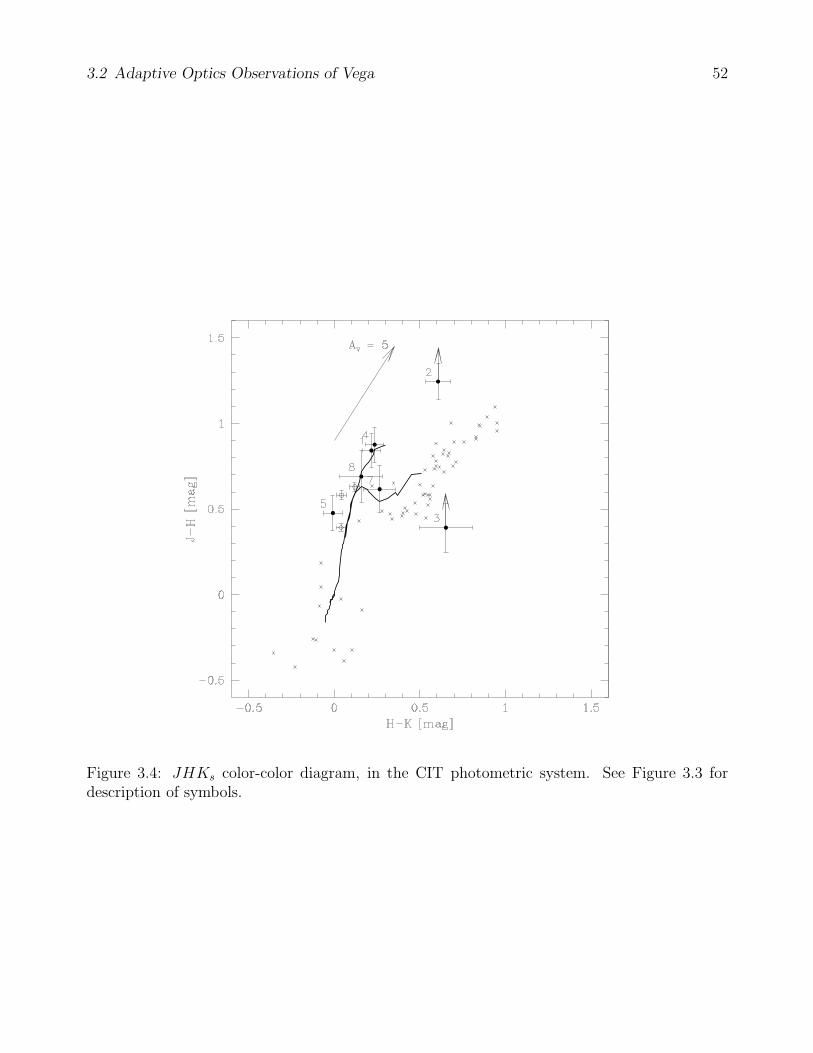
3.2 Adaptive Optics Observations of Vega 52
Figure 3.4: JHKs color-color diagram, in the CIT photometric system. See Figure 3.3 fordescription of symbols.

3.2 Adaptive Optics Observations of Vega 53
dust clumps around Vega. Spectral energy distributions of (sub-)millimeter galaxies (Danner-bauer et al., 2002; Goldader et al., 2002; Klaas et al., 2001) suggest z &1 for any responsiblebackground galaxy, given our non-detection at H band. However, deep searches for K-bandcounterparts to several sub-millimeter galaxies have reached K ≈ 22 mag (e.g., Dannerbaueret al., 2002) with no counterpart detection, suggesting that our data may be too insensitive (by6–7 magnitudes at these locations) to put a sensible limit on this hypothesis.
3.2.7 Conclusions
We find 8 faint objects within 35′′ of Vega that are 15–19 mag fainter than the star at H-band.If associated, at the 330 Myr age for Vega, current brown-dwarf cooling models (Burrows et al.,2001; Chabrier et al., 2000) set their masses at 5–35 MJup. The number of detected objectsis however consistent with estimates of field star density, and their colors and proper motionindicate that they are not associated with Vega.
We thus exclude the possibility of a distant (80–220 AU; ∼83% of this area is imaged),massive (>10 MJup; >6 MJup for 120–220 AU) planetary/brown-dwarf companion causing theobserved dust distribution around Vega. We also detect nothing at the positions of the predictedplanetary perturbers, with upper mass limits 7–15 MJup (H<17–13), well above the 2–3 MJup
predictions. We detect nothing at the position of the mid-infrared dust clumps, placing limitson the possibility of their extragalactic interpretation.

3.3 Initial Results from the PALAO Survey of Young Solar-type Stars 54
3.3 Initial Results from the PALAO Survey of Young
Solar-type Stars
†Stanimir A. Metchev & Lynne A. Hillenbrand
California Institute of Technology, Division of Physics, Mathematics & Astronomy, MC 105–24, Pasadena,California 91125
Abstract
We present first results from the Palomar Adaptive Optics Survey of Young Stars conductedat the Hale 5 m telescope. Through direct imaging we have discovered a brown dwarf and twolow-mass stellar companions to the young solar-type stars HD 49197, HD 129333 (EK Dra),and V522 Per, and confirmed a previously suspected companion to RX J0329.1+0118 (Sterziket al., 1997), at respective separations of 0.95′′ (43 AU), 0.74′′ (25 AU), 2.09′′ (400 AU), and3.78′′ (380 AU). Physical association of each binary system is established through commonproper motion and/or low-resolution infrared spectroscopy. Based on the companion spectraltypes, we estimate their masses at 0.06, 0.20, 0.13, and 0.20 M, respectively. From analysisof our imaging data combined with archival radial velocity data, we find that the spatiallyresolved companion to HD 129333 is potentially identical to the previously identified spectro-scopic companion to this star (Duquennoy & Mayor, 1991). However, a discrepancy with theabsolute magnitude suggests that the two companions could also be distinct, with the resolvedone being the outermost component of a triple system.2 The brown dwarf HD 49197B is anew member of a growing list of directly imaged sub-stellar companions at 10–1000 AU separa-tions from main sequence stars, indicating that such brown dwarfs may be more common thaninitially speculated.
3.3.1 Introduction
High-contrast imaging searches for low-mass companions to nearby and/or young stars haveincreased dramatically in number since the initial discovery of a brown-dwarf companion to amain sequence star (Gl 229) through direct imaging (Nakajima et al., 1995). One particularlypowerful technique is adaptive optics (AO), which provides the high angular resolution (. 0.1′′)achievable at the diffraction limit of large ground-based telescopes. The widening niche of high-contrast imaging opened by recent developments in AO technology implies that not only browndwarfs but exo-solar planets may be within the realm of direct imaging. Nowadays nearlyevery ground-based telescope equipped with an AO system hosts an imaging companion-search
†A version of this Section was published in The Astrophysical Journal, vol. 617, 13302More detailed radial-velocity and direct-imaging monitoring of HD 129333, subsequently published in Konig
et al. (2005), has shown that the system is a binary. The dynamical masses of the components are 0.9± 0.1M
and 0.5±0.1M. The secondary mass reported in Konig et al. is consistent with the one inferred in the presentwork (Metchev & Hillenbrand, 2004). The ambiguity in the multiplicity in the present case is rooted in theassumption of a fixed mass for the primary (§3.3.4.3.1)–a necessary step given the insufficient number of orbitalconstraints. The adopted fixed mass (1.05M) was too large, compared to the one found from Konig et al.’sbetter constrained orbital solution.

3.3 Initial Results from the PALAO Survey of Young Solar-type Stars 55
project. The sudden explosion in interest in this topic has been fueled by the success of theradial velocity (r.v.) method in detecting solar system analogs (e.g., Marcy & Butler, 1998).Through longer time-lines of observation and higher precision, the sensitivity of r.v. surveyshas now extended outwards to include planets at semi-major axes &3 AU (Carter et al., 2003;Naef et al., 2004), i.e., near the Jovian region in the Solar System. While the sensitivity ofdirect imaging to “planetary-mass” (1–13 Jupiter masses (MJ); Burrows et al., 1997) objectsat such separations from Sun-like stars is still extremely limited due to contrast requirements,several higher-mass brown-dwarf companions have been discovered at wider separations (seecompilation in Reid et al., 2001), some at projected distances as small as 14–19 AU (Els et al.,2001; Liu et al., 2002). High-resolution spectroscopic monitoring and direct imaging are thuscomplementary in searching for sub-stellar companions to stars. Future development of bothmethods promises to narrow, and eventually close, the sensitivity gap between them.
Young stars are the most suitable targets for direct imaging of sub-stellar companions. Atages of 10–100 million years (Myr) the expected brightness ratio in the near IR between a10 MJup object and a solar-type star is 10−3–10−5 (Burrows et al., 1997; Baraffe et al., 2003).Modern AO systems can routinely achieve comparable dynamic range at 1′′ separations frombright stars. Hence, for young stars within 40 pc of the Sun we can probe for massive planets atseparations comparable to the giant planet region in our own Solar System. However, few youngstars are known at such small heliocentric distances. These are constrained to several tens ofmembers of young moving groups: TW Hya (Rucinski & Krautter, 1983; de La Reza et al.,1989), Tucana/Horologium (Zuckerman & Webb, 2000; Zuckerman et al., 2001a), and β Pic(Zuckerman, Song, & Webb, 2001b), and have already been targeted with sensitive space-basedand ground-based AO surveys, which have uncovered 3–4 brown-dwarf companions (Lowrance,2001; Lowrance et al., 2003; Neuhauser & Guenther, 2004), but no planetary-mass ones.
Because contrast and projected separation are the limiting factors in detectability of sub-stellar companions, brown dwarfs, being more luminous than planets, are detectable at greaterheliocentric distances and at smaller angular separations from their host stars. At the samephysical separation from the primary (e.g., 50–100 AU), brown-dwarf companions should bedetectable around older (several gigayears [Gyr]) and/or more distant (.200 pc) stars comparedto planets, allowing a larger sample of targets. With regard to this, we have commenced asurvey of young (<500 Myr) solar-type (F5–K5) stars within 200 pc using the AO system onthe Palomar 5-m telescope. Our survey sample is largely a subset of the sample targeted bythe Formation and Evolution of Planetary Systems (FEPS) Spitzer Legacy Team (Meyer et al.,2004). Although faint primary stars, such as M dwarfs or white dwarfs, offer more favorablecontrast for imaging sub-stellar companions, we have chosen to limit our sample to solar analogsbecause of interest in determining the multiplicity statistics of sub-stellar objects around othersuns. Furthermore, several recent large surveys have already explored the multiplicity of nearby(.50 pc) cool stars (Close et al., 2003; Carson et al., 2003; McCarthy & Zuckerman, 2004) orwhite dwarfs (Zuckerman & Becklin, 1992; Green, Ali, & Napiwotzki, 2000), while a large sampleof F–G stars has not been studied because of comparatively small numbers in the immediatesolar neighborhood.
Preliminary results from our survey were reported in Metchev, Hillenbrand, & Meyer (2002).Here we present the strategy of the survey, and the discovery and confirmation of resolvedlow-mass companions to HD 49197, HD 129333 (EK Dra), V522 Per, and RX J0329.1+0118.We shall refer to these throughout the paper as HD 49197B, HD 129333B, V522 PerB, andRX J0329.1+0118B. For convenience of notation, a second candidate companion to HD 49197
3.3 Initial Results from the PALAO Survey of Young Solar-type Stars 56
found to be an unrelated background star will be denoted as HD 49197“C”. The full sampleand further results from the survey will be discussed in a later paper.
3.3.2 Observing Strategy
The observations described in this section are representative of our general survey observingstrategy. Table 3.2 details the imaging and spectroscopic observations specifically for the fourobjects presented here. The properties of the observed primaries are given in Table 3.3.
3.3.2.1 Imaging
3.3.2.1.1 First-Epoch Imaging and Survey Sample Subdivision
First epoch observations are obtained with the Palomar AO system (PALAO; Troy et al.,2000) in residence at the Cassegrain focus of the Palomar 5-m telescope. Since the summer of2003 the wavefront sensor runs at frame rates up to 2 kHz, and the system routinely producesdiffraction-limited images (0.09′′ at KS) with Strehl ratios3 in the 30–50% range at 2µm onV < 12 guide stars and up to 75% on V < 7 mag guide stars. PALAO employs the PalomarHigh Angular Resolution Observer (PHARO; Hayward et al., 2001), a 1024×1024 pix HgCdTeHAWAII detector with imaging (25 mas/pix and 40 mas/pix pixel scale) and spectroscopic(R=500–2000) capabilities in the near IR. A set of coronagraphic spots, Lyot masks and neutraldensity (ND) filters are available to achieve the desired dynamic range.
Our program entails KS-band (2.15µm) imaging in the 25 mas/pix mode (25′′ × 25′′ field ofview) both with and without a 0.97′′-diameter coronagraphic stop. For high dynamic range, long(1 min) coronagraphic images are taken to identify fainter (potentially sub-stellar) companionsat separations >0.5′′. Twenty-four such exposures are taken, for a total of 24 min integrationper target, with 6 min spent at each of 4 different orthogonal detector orientations (obtainedby rotating the Cassegrain ring of the telescope). For every 6 min of on-target imaging (i.e., ateach detector orientation), separate 1-min coronagraphic exposures are taken at five ditheredsky positions 32–60′′ from the star. For high angular resolution (but with lower dynamicrange), short (1.4–9.8 sec) non-coronagraphic exposures are taken to look for close companionsof modest flux ratio and to establish relative photometric calibration. The images are taken ina 5-point dither pattern at the vertices and center of a box 6′′ on a side. A 1%-transmission NDfilter is used if necessary to avoid saturation4. On occasion, a narrow-band (1%) Brackett-γ(2.17µm) filter is used for higher throughput, instead of the ND 1% filter.
To avoid detector saturation and/or decreased sensitivity over a substantial fraction of theimage area, stars with bright (∆KS < 4) projected companions in the PHARO field of view(FOV) were not observed with deep coronagraphic exposures. However, binaries with separa-tion ≤ 0.5′′ were included, as both components of the binary could then be occulted by thecoronagraph. This naturally splits our survey sample in two groups: the “deep” subsample,
3The Strehl ratio is an empirical measure of the quality of an image, equal to the ratio of the peak of theobserved PSF to the peak of the ideal, diffraction-limited, telescope PSF. High-order AO systems nowadaysroutinely achieve Strehl ratios >50% at K-band.
4The ND 1% filter was calibrated photometrically through repeated (17–20 per band) observations of3 program stars with and without the filter, and its extinction was measured at 4.753±0.039 mag at J ,4.424±0.033 mag at H , and 4.197±0.024 mag at KS .

3.3In
itialR
esults
fromth
ePA
LA
OSurvey
ofY
oung
Solar-ty
pe
Stars
57
Table 3.2: ObservationsTarget First Epoch/Telescope Mode Second Epoch/Telescope Mode
HD 49197 2002 Feb 28/Palomar JHKS coronagraphic imaging 2003 Nov 9–10/Keck II JHKS coronagraphic imaging,K spectroscopy
HD 129333 2003 Jan 12/Palomar JHKS non-coronagraphic imaging, 2003 May 13/Palomar Brγ non-coronagraphic imagingJK spectroscopy
V522 Per 2003 Sep 20/Palomar JHKS non-coronagraphic imaging 2003 Nov 10/Keck II KSL′ non-coronagraphic imaging,
JK spectroscopyRX J0329.1+0118 2003 Sep 21/Palomar JHKS coronagraphic imaging 2003 Nov 10/Keck II K spectroscopy
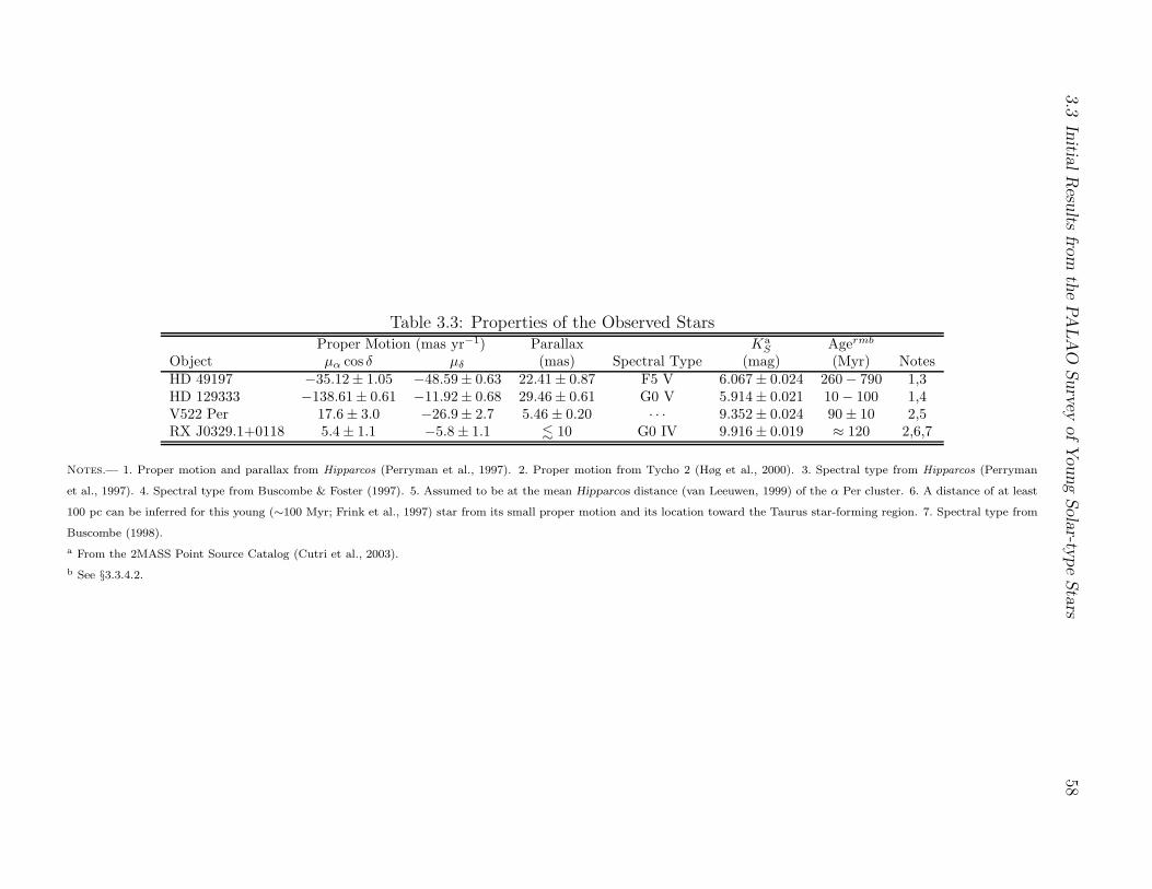
3.3In
itialR
esults
fromth
ePA
LA
OSurvey
ofY
oung
Solar-ty
pe
Stars
58
Table 3.3: Properties of the Observed StarsProper Motion (mas yr−1) Parallax Ka
SAgermb
Object µα cos δ µδ (mas) Spectral Type (mag) (Myr) NotesHD 49197 −35.12± 1.05 −48.59± 0.63 22.41± 0.87 F5 V 6.067 ± 0.024 260 − 790 1,3HD 129333 −138.61± 0.61 −11.92± 0.68 29.46± 0.61 G0 V 5.914 ± 0.021 10 − 100 1,4V522 Per 17.6 ± 3.0 −26.9± 2.7 5.46 ± 0.20 · · · 9.352 ± 0.024 90 ± 10 2,5RX J0329.1+0118 5.4 ± 1.1 −5.8 ± 1.1 . 10 G0 IV 9.916 ± 0.019 ≈ 120 2,6,7
Notes.— 1. Proper motion and parallax from Hipparcos (Perryman et al., 1997). 2. Proper motion from Tycho 2 (Høg et al., 2000). 3. Spectral type from Hipparcos (Perryman
et al., 1997). 4. Spectral type from Buscombe & Foster (1997). 5. Assumed to be at the mean Hipparcos distance (van Leeuwen, 1999) of the α Per cluster. 6. A distance of at least
100 pc can be inferred for this young (∼100 Myr; Frink et al., 1997) star from its small proper motion and its location toward the Taurus star-forming region. 7. Spectral type from
Buscombe (1998).
a From the 2MASS Point Source Catalog (Cutri et al., 2003).
b See §3.3.4.2.
3.3 Initial Results from the PALAO Survey of Young Solar-type Stars 59
consisting of essentially single stars and close binaries, and the “shallow” subsample encom-passing the remaining stars. Membership to one of the two subsamples was assigned at thetelescope, when their multiplicity and approximate flux ratio was revealed during the shortexposures. The shallow subsample was further expanded to include stars out to 200 pc and/orolder than 500 Myr to cover the entire FEPS sample accessible from the Northern hemisphere.
Short dithered exposures were taken of all stars, while long coronagraphic exposures weretaken only of stars in the deep subsample at KS band. In addition, short J- (1.22µm) and H-band (1.65µm) exposures were taken of all candidate binaries (all stars in the shallow survey,and the < 0.5′′ systems in the deep survey) to allow approximate photospheric characterizationof the components.
In accordance with the above distinction, HD 49197 was observed for a total of 24 minwith the coronagraph as a part of the deep survey, while HD 129333 and RX J0329.1+0118(with bright candidate companions), and V522 Per (α Per member, 190 pc from the Sun; vanLeeuwen, 1999) were observed only with short exposures. Conditions were photometric duringthe first epoch observations of HD 49197, V522 Per, and RX J0329.1+0118, and unstable duringthose of HD 129333.
3.3.2.1.2 Follow-Up Imaging
We obtain second-epoch imaging observations of all candidate companions to check forcommon proper motion with their corresponding stars. Such were taken for HD 129333 withPALAO/PHARO, and for HD 49197, V522 Per, and RX J0329.1+0118 with NIRC2 (Matthewset al., in prep.) and the Keck II AO system (diffraction limit 0.05′′ at KS; Wizinowich et al.,2000). Conditions were not photometric during follow-up, and only the best images (Strehlratio S & 40%) were selected for astrometry. HD 129333 was followed up in the narrow-band Brackett γ filter, which allowed higher throughput than the ND 1% filter in the shortest(1.4 sec) PHARO exposures. Given the unstable atmospheric conditions during the second-epoch imaging of HD 129333, this allowed us to take high signal-to-noise (S/N) exposures ontime-scales that would most finely sample the variations in the seeing and to select only theones with the best imaging quality.
Keck follow-up is done at JHKS, or at KSL′ if the candidate companion is expected to be
bright enough to be seen at L′ (given 0.7 < KS − L′ < 2.5 for L and T dwarfs; Leggett et al.,2002). Sequences of short (up to 20 sec from multiple co-adds) dithered non-coronagraphic andlong (1 min) target-sky-target exposures are taken with a 1′′- or 2′′-diameter coronagraph in thesame manner as with PHARO, though without detector rotations. The candidate companionsare exposed until a S/N ratio comparable to that in the first-epoch PHARO observation isachieved (for similar positional accuracy), up to 6 min per filter in J , H , and KS. The totalintegration time at L′ is up to 10.5 min, which allows the detection of L′ . 15.0 objects. Wemainly use the 40 mas/pix (wide) NIRC2 camera (41′′ FOV), which severely under-samplesthe Keck AO point-spread function (PSF), but is known to suffer from less distortion thanthe 20 mas/pix (medium) camera over the same field (Thompson, Egami, & Sawicki, 2001).Although we also have the option of using the 10 mas/pix (narrow) camera (10′′ FOV) inNIRC2, it does not allow follow-up of distant candidate companions, and we avoid using it forconsistency with the other NIRC2 observations.

3.3 Initial Results from the PALAO Survey of Young Solar-type Stars 60
(c)
Keck 1" (45 AU)
(b)
Palomar 1" (45 AU)
(a)
Palomar 3" (135 AU)
E
N
Figure 3.5: KS-band (2.15µm) first (a, b) and second (c) epoch images of HD 49197. Panel(a) shows both candidate companions to HD 49197; panels (b) and (c) are zoomed in to pointout only the close-in, bona fide companion (HD 49197B). The first-epoch image is the result of24 median-combined 60 sec exposures with Palomar/PHARO, whereas the second-epoch imagewas formed by median-combining six 60 sec exposures with Keck/NIRC2. A 1.0′′-diametercoronagraph occults the primary in both cases; in the Keck image the coronagraph shows aresidual ≈0.16% transmission. HD 49197B was initially unnoticed in the first-epoch image,where its detection was hindered by the presence of equally prominent AO speckles.
3.3.2.1.3 Imaging Data Reduction
All imaging data are reduced in a standard fashion for near IR observations. Flat fieldsare constructed either from images of the twilight sky (for the Palomar data) or from imagesof the lamp-illuminated dome interior (for the Keck data). A bad pixel mask is created fromthe individual flats, based on the response of each pixel to varying flux levels. Pixels whosegain deviates by more than 5 sigma from the mode gain of the array are flagged as bad. Skyframes for the dithered, non-coronagraphic exposures are obtained by median-combining fourof the five exposures in the dither pattern (excluding the central pointing) and rejecting thehighest pixel value in the stack. The coronagraphic-mode sky frames are median-combinedusing an average sigma clipping algorithm to remove pixels deviant by more than 5 sigma. Thesky-subtracted images of each target are divided by the flat field, then registered and median-combined to create a final high signal-to-noise (S/N) image (Figures 3.5 and 3.6). However,photometric and astrometric measurements are performed on the individual reduced images.
No PSF stars are observed at either Palomar or Keck. With PHARO at Palomar, median-combined images from all 4 detector orientations can be used to reproduce an approximatePSF. This approach was chosen to emulate the observation of separate PSF stars of identicalbrightness and color, while optimizing the time spent on science targets. However, we havefound that a simple 180 rotation and subtraction technique works equally well, and we usethat on both the Palomar and Keck data. While neither approach eliminates telescopic specklenoise (as could be the case if actual PSF stars were observed), both significantly reduce point-symmetric structure in the PSF.
3.3.2.2 Astrometric Calibration
The exact pixel scale of the 25 mas PHARO camera was determined using known binary starsfrom the Sixth Orbit Catalog (Hartkopf, Mason, & Worley, 2001; Hartkopf & Mason, 2003):

3.3 Initial Results from the PALAO Survey of Young Solar-type Stars 61
E
N
HD 129333
2" (68 AU) E
N
V522 Per
2" (380 AU) E
N
RX J0329.1+0118
2" (200 AU)
Figure 3.6: Palomar images of the stellar companions. The HD 129333 image is taken througha narrow-band (1%) Brγ (2.166 µm) filter, while the V522 Per and RX J0329.1+0118 imagesare taken at KS. Five dithered 1.4 sec exposures were aligned and median-combined to obtaineach of the displayed images.
WDS 09006+4147 (grade 1; Hartkopf, Mason, & McAlister, 1996), WDS 16147+3352 (grade 4;Scardia, 1979), WDS 18055+0230 (grade 1; Pourbaix, 2000), and WDS 20467+1607 (grade 4;Hale, 1994). These “calibration binaries” are observed throughout our campaign at Palomarat all four detector orientations. The combination of grade 1 (accurately determined, short-period) orbits and grade 4 (less accurately known, longer-period) orbits was selected from thelist of astrometric calibrators recommended by Hartkopf & Mason (2003). Despite the lowerquality of the solution for binaries with grade 4 orbits, their periods are generally much longer(889 and 3249 years for WDS 16147+3352 and WDS 20467+1607 vs. 21.78 and 88.38 yearsfor WDS 09006+4147 and WDS 18055+0230, respectively), so their motions are predictedwith sufficient accuracy for many years into the future. The mean pixel scale of PHARO wasmeasured to be 25.22 mas/pix with a 1 sigma scatter of 0.11 mas/pix among measurementsof the individual binaries at different detector orientations. This measurement is consistentwith, though less precise than, our previous determination (25.168 ± 0.034 mas/pix; Metchev,Hillenbrand, & White, 2003), which was obtained from only one calibration binary at a singleCassegrain ring orientation. The larger scatter of our more recent measurement is indicativeof the systematics involved in choosing different calibration binaries and in observing at morethan one detector orientation.
The pixel scale of the wide NIRC2 camera was calibrated using the binary WDS 15360+3948(grade 1; Soderhjelm, 1999). The obtained value of 39.82±0.25 mas/pix is consistent with thepre-ship measurement of 39.7±0.5 max/pix5. Because only one binary was used for calibratingNIRC2, a 0.63% error term corresponding to the uncertainty in the semi-major axis of thebinary has been added in quadrature to the uncertainty of our measurement.
3.3.2.3 Spectroscopy
3.3.2.3.1 Observations
Spectroscopy of faint targets in the halos of bright objects is more challenging than spec-troscopy of isolated targets. Care needs to be taken to achieve optimum suppression of thescattered light of the bright stars either by using a coronagraph (in a manner similar to coron-
5See http://www2.keck.hawaii.edu/inst/nirc2/genspecs.html.

3.3 Initial Results from the PALAO Survey of Young Solar-type Stars 62
agraphic imaging) or by aligning the slit so as to minimize light admitted from the halo. Sinceneither PHARO nor NIRC2 allow coronagraphic spectroscopy, when taking spectra of faintcompanions we orient the slit as close as possible to 90 from the primary-companion axis.Spectra of brighter companions, for which the signal from the halo is negligible compared tothat from the target, are obtained by aligning the binary along the slit. Given that we oftenuse the F5–K5 IV–V primaries in our sample as telluric standards, such alignment improvesour observing efficiency. Sky spectra are obtained simultaneously with the target spectra bydithering the targets along the slit.
Promising candidate companions are observed at medium resolution (R = 1000 − 3000)at K and (AO correction permitting) at J . In PHARO we use the corresponding grism andfilter combination (K or J) and the 40 mas/pix camera, while in NIRC2 we use the K or Jfilter with the “medres” grism, and the wide (40 mas/pix) camera. For K-band spectroscopyin first order with PHARO and in fifth order with NIRC2 we achieve complete coverage of the2.2µm atmospheric window. For J-band spectroscopy in first order with PHARO the coverageis limited by the size of the detector to a 0.16µm bandwidth. J-band spectroscopy with NIRC2can cover the entire 1.2µm window, but the spectrum is split between the fifth and the sixthdispersion orders. To allow simultaneous data acquisition from both orders, we fit both onto thewide camera by clipping the fifth (longer-wavelength) order shortward of 1.22µm and the sixth(shorter-wavelength) order longward of 1.28µm. The combined J-band spectrum has completecoverage between 1.16–1.35µm.
We took J and K-band spectra with PHARO of HD 129333A/B, J and K spectra withNIRC2 of V522 PerA/B, and K-band NIRC2 spectra of HD 49197A/B and RX J0329.1 +0118A/B. For the observations of HD 129333 with PHARO and of RX J0329.1+0118 withNIRC2, the binary was aligned along the slit, whereas spectra of the other two binaries (withfainter companions) were obtained by placing each component in the slit individually. A 0.26′′
(6.5 pix) slit was used in PHARO, and a 0.08′′ (2 pix) slit was used in NIRC2, resulting inspectral resolutions of 1200 at J and 1000 at K with PHARO, and 2400 at fifth-order J (1.22–1.35µm), 2900 at sixth-order J (1.15–1.28µm), and 2700 at K with NIRC2.
Flat fields with the dispersive grisms in place were not obtained for any of our spectroscopicobservations. Instead, the raw spectra were divided by an imaging flat field, constructed inthe same manner as for the imaging observations. The flat-fielded spectra were corrected forbad pixels, using the same bad pixel mask as in the imaging case. Strong positive deviationsdue to cosmic ray hits were then eliminated using the L.A. Cosmic Laplacian filter algorithm(van Dokkum, 2001). Fringing was at a noticeable level (≈15%) only in spectra obtained withPHARO (of HD 129333) and was reduced to below 5% by dividing the target spectrum by thatof the telluric standard, taken at a nearby position on the detector.
3.3.2.3.2 Spectroscopic Data Reduction
Extraction of the spectra is performed using iraf/apextract tasks. To reduce contam-ination from the halo of the primary in the companion spectra, the local background (arisingmostly from the halo) is fit by a first-order polynomial along the direction perpendicular tothe dispersion axis and subtracted during extraction. In addition, the aperture width for thecompanion spectrum is conservatively set to the full width at half maximum of the profile so asto include only pixels with maximum signal-to-noise. Pixels within the aperture are summedalong detector columns (which are nearly perpendicular to the dispersion axis), and the re-

3.3 Initial Results from the PALAO Survey of Young Solar-type Stars 63
sulting “compressed” spectrum is traced along the dispersion axis by fitting a high order (8to 15) Legendre polynomial. The tracing step is approximately equal to the slit width, whereat each step the data point is obtained as the sum of 3–10 adjacent pixels (1.5–3 slit widths;the spectra of fainter objects being more heavily averaged) in the compressed spectrum. Thisprocedure is found to produce consistent results for extractions of multiple dithered spectraof the same companion, indicating that scattered light contamination from the primary hasbeen reduced to a small level. Nevertheless, in some cases of very faint close-in companions,the continuum shape is still found to vary noticeably among the individual extractions. Wetherefore avoid classifying the spectra of the companions based on their continuum shapes, butrely on the relative strengths of narrow absorption features (discernible given our resolution)instead (§3.3.3.3).
A dispersion solution for each spectrum is obtained from night sky lines in non-sky-subtractedimages, using the task identify and OH emission-line lists available in iraf. For the spectraof primaries observed separately (e.g., HD 49197 and V522 Per), whose shallower (10–120 sec)exposures do not contain telluric emission lines at a high enough S/N to allow the fitting of adispersion solution, such is derived after registration with deeper (10–15 min long) companionspectra taken immediately after those of the primaries. The tasks fxcor and specshift areused to cross-correlate and align the individual wavelength-calibrated spectra for a given object.The individual primary and companion spectra are then median-combined using scombine.
Since the primaries (when earlier than K0) double as telluric standards, their spectra arefirst corrected for photospheric absorption from atomic hydrogen (H Pβ at 1.282µm and H Brγat 2.166µm) by hand-interpolating over the absorption with the task splot. Weaker absorp-tion features due to Na I, Ca I, Si I, Al I, and Fe I, although present in the spectra of ourtelluric standards, are left uncorrected because of blending (at our resolution) with variousOH absorption lines in the Earth’s atmosphere. After thus correcting the telluric spectra, thespectra of the companions are divided by those of the telluric standards. Finally, the spectra ofthe companions are multiplied by black bodies with temperatures corresponding to the spectraltypes of the telluric standards (based on effective temperature vs. spectral type data from Cox,2000) and boxcar-smoothed by the width of the slit.
The above reduction procedure applies in exact form for NIRC2 spectra, which do not sufferfrom fringing. For PHARO data, which are noticeably affected by fringing, we divide the indi-vidual target spectra by those of the telluric standard before median-combining and wavelengthcalibration, since fringing depends on detector position, not on the dispersive element.
Reduced spectra for the objects reported here are presented in Figure 3.7 and 3.8. Themismatch in the continuum slopes between the fifth- and sixth-order J-band spectra of thecompanion to V522 Per may be due to our use of imaging, instead of spectroscopic flats.
3.3.3 Analysis
3.3.3.1 Photometry
Broad-band near-IR photometry of the companions is presented in Table 3.4. The measuredquantity in each case is the relative flux (∆J , ∆H , ∆KS , ∆L′) of the companion with respectto that of the primary. When the companions were visible without the coronagraph (in all casesexcept for the close-in companion to HD 49197), the fluxes of both components were measureddirectly from the short-exposure non-coronagraphic images. Flux ratios for the HD 129333,

3.3 Initial Results from the PALAO Survey of Young Solar-type Stars 64
Figure 3.7: K-band spectra of the low-mass companions from Palomar (HD 129333B;R ≈ 1000)and Keck (RX J0329.1+0118B, V522 PerB, and HD 49197B; R ≈ 2700). All spectra have beennormalized to unity at 2.20µm and offset by 0.5 in the vertical axis.

3.3 Initial Results from the PALAO Survey of Young Solar-type Stars 65
Figure 3.8: J-band spectra of two of the low-mass companions from Palomar (HD 129333B;R ≈ 1200) and Keck (V522 PerB; R ≈ 2400 in the fifth order and R ≈ 2900 in the sixth). Allspectra have been normalized to unity at 1.25µm and offset by 0.5 in the vertical axis.
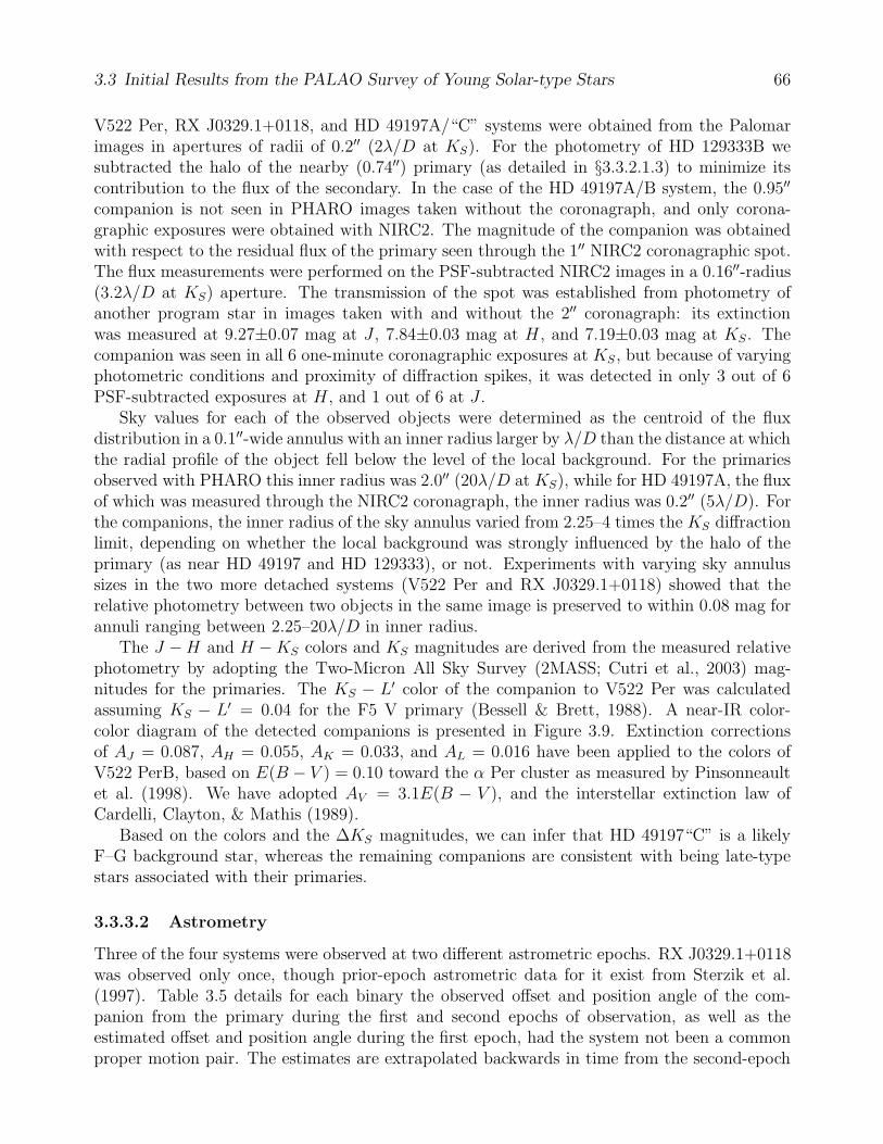
3.3 Initial Results from the PALAO Survey of Young Solar-type Stars 66
V522 Per, RX J0329.1+0118, and HD 49197A/“C” systems were obtained from the Palomarimages in apertures of radii of 0.2′′ (2λ/D at KS). For the photometry of HD 129333B wesubtracted the halo of the nearby (0.74′′) primary (as detailed in §3.3.2.1.3) to minimize itscontribution to the flux of the secondary. In the case of the HD 49197A/B system, the 0.95′′
companion is not seen in PHARO images taken without the coronagraph, and only corona-graphic exposures were obtained with NIRC2. The magnitude of the companion was obtainedwith respect to the residual flux of the primary seen through the 1′′ NIRC2 coronagraphic spot.The flux measurements were performed on the PSF-subtracted NIRC2 images in a 0.16′′-radius(3.2λ/D at KS) aperture. The transmission of the spot was established from photometry ofanother program star in images taken with and without the 2′′ coronagraph: its extinctionwas measured at 9.27±0.07 mag at J , 7.84±0.03 mag at H , and 7.19±0.03 mag at KS. Thecompanion was seen in all 6 one-minute coronagraphic exposures at KS, but because of varyingphotometric conditions and proximity of diffraction spikes, it was detected in only 3 out of 6PSF-subtracted exposures at H , and 1 out of 6 at J .
Sky values for each of the observed objects were determined as the centroid of the fluxdistribution in a 0.1′′-wide annulus with an inner radius larger by λ/D than the distance at whichthe radial profile of the object fell below the level of the local background. For the primariesobserved with PHARO this inner radius was 2.0′′ (20λ/D at KS), while for HD 49197A, the fluxof which was measured through the NIRC2 coronagraph, the inner radius was 0.2′′ (5λ/D). Forthe companions, the inner radius of the sky annulus varied from 2.25–4 times the KS diffractionlimit, depending on whether the local background was strongly influenced by the halo of theprimary (as near HD 49197 and HD 129333), or not. Experiments with varying sky annulussizes in the two more detached systems (V522 Per and RX J0329.1+0118) showed that therelative photometry between two objects in the same image is preserved to within 0.08 mag forannuli ranging between 2.25–20λ/D in inner radius.
The J −H and H −KS colors and KS magnitudes are derived from the measured relativephotometry by adopting the Two-Micron All Sky Survey (2MASS; Cutri et al., 2003) mag-nitudes for the primaries. The KS − L′ color of the companion to V522 Per was calculatedassuming KS − L′ = 0.04 for the F5 V primary (Bessell & Brett, 1988). A near-IR color-color diagram of the detected companions is presented in Figure 3.9. Extinction correctionsof AJ = 0.087, AH = 0.055, AK = 0.033, and AL = 0.016 have been applied to the colors ofV522 PerB, based on E(B − V ) = 0.10 toward the α Per cluster as measured by Pinsonneaultet al. (1998). We have adopted AV = 3.1E(B − V ), and the interstellar extinction law ofCardelli, Clayton, & Mathis (1989).
Based on the colors and the ∆KS magnitudes, we can infer that HD 49197“C” is a likelyF–G background star, whereas the remaining companions are consistent with being late-typestars associated with their primaries.
3.3.3.2 Astrometry
Three of the four systems were observed at two different astrometric epochs. RX J0329.1+0118was observed only once, though prior-epoch astrometric data for it exist from Sterzik et al.(1997). Table 3.5 details for each binary the observed offset and position angle of the com-panion from the primary during the first and second epochs of observation, as well as theestimated offset and position angle during the first epoch, had the system not been a commonproper motion pair. The estimates are extrapolated backwards in time from the second-epoch
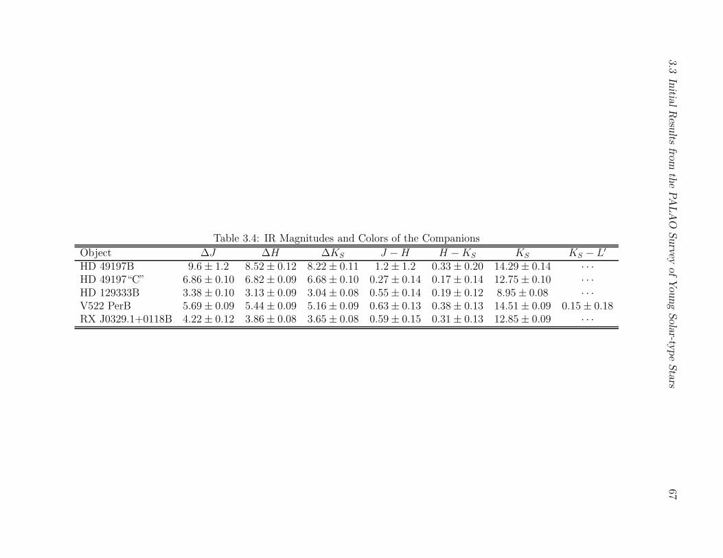
3.3In
itialR
esults
fromth
ePA
LA
OSurvey
ofY
oung
Solar-ty
pe
Stars
67
Table 3.4: IR Magnitudes and Colors of the Companions
Object ∆J ∆H ∆KS J −H H −KS KS KS − L′
HD 49197B 9.6 ± 1.2 8.52 ± 0.12 8.22 ± 0.11 1.2 ± 1.2 0.33 ± 0.20 14.29 ± 0.14 · · ·HD 49197“C” 6.86 ± 0.10 6.82 ± 0.09 6.68 ± 0.10 0.27 ± 0.14 0.17 ± 0.14 12.75 ± 0.10 · · ·HD 129333B 3.38 ± 0.10 3.13 ± 0.09 3.04 ± 0.08 0.55 ± 0.14 0.19 ± 0.12 8.95 ± 0.08 · · ·V522 PerB 5.69 ± 0.09 5.44 ± 0.09 5.16 ± 0.09 0.63 ± 0.13 0.38 ± 0.13 14.51 ± 0.09 0.15 ± 0.18RX J0329.1+0118B 4.22 ± 0.12 3.86 ± 0.08 3.65 ± 0.08 0.59 ± 0.15 0.31 ± 0.13 12.85 ± 0.09 · · ·

3.3 Initial Results from the PALAO Survey of Young Solar-type Stars 68
]
Figure 3.9: Near-IR color-color diagram of the detected companions. The solid line representsthe B2V–L8V main sequence, with data compiled from Cox (2000, B2V–M6V) and Kirkpatricket al. (2000, M8V–L8V). The dashed line shows the G0–M7 giant branch (Cox, 2000). TheCox and the Kirkpatrick et al. colors are converted from the Johnson-Glass (Bessell & Brett,1988) and 2MASS (Cutri et al., 2003) systems, respectively, to the CIT system using relationsfrom Carpenter (2001). HD 49197“C” is too blue to be a bona fide low-mass companion toHD 49197. The near IR colors of the remainder of the companions agree well with their inferredspectral types (Table 3.7).

3.3In
itialR
esults
fromth
ePA
LA
OSurvey
ofY
oung
Solar-ty
pe
Stars
69
Table 3.5: Astrometry of the CompanionsEpoch 1 Epoch 2 Epoch 1 if Non-common Proper Motion
Offset P.A. Offset P.A. Offset P.A.Object (arcsec) (degrees) (arcsec) (degrees) (arcsec) (degrees)HD 49197B 0.9499±0.0054 78.25±0.40 0.9475±0.0022 77.60±0.25 0.9029±0.0037 81.87±0.31HD 49197“C” 6.971±0.030 346.13±0.34 7.016±0.008 346.50±0.10 6.950±0.009 346.10±0.10HD 129333B 0.7343±0.0032 173.19±0.35 0.7363±0.0032 173.37±0.35 0.7221±0.0033 180.68±0.37V552 PerB 2.0970±0.0090 194.02±0.34 2.0937±0.0032 193.91±0.11 2.0991±0.0032 193.93±0.11RX J0329.1+0118B 3.75±0.05 303±5 3.781±0.016 303.85±0.34 3.714±0.070 303.7±1.1

3.3 Initial Results from the PALAO Survey of Young Solar-type Stars 70
Figure 3.10: Proper motion diagram for the two companions to HD 49197. The offsets from theprimary at each observational epoch are plotted as solid points with errorbars. The inferredoffsets at the first epoch (assuming non-common proper motion) are shown just with errorbars.The dashed lines reflect the proper and parallactic motions of the primary between the twoepochs. HD 49197B is a common proper motion companion within the 1 sigma errors, whileHD 49197“C” is more consistent with being a background object.
astrometry, which for all except HD 129333 was obtained with NIRC2 on Keck and was moreaccurate, assuming proper motions from Hipparcos (Perryman et al., 1997) for HD 49197 andHD 129333, and from Tycho 2 (Høg et al., 2000) for V522 Per and RX J0329.1+0118. Paral-lactic motions were also taken into account, as they are significant for stars . 200 pc at ourastrometric precision (several milli-arcsec). The assumed proper motions and parallaxes for allstars are listed in Table 3.3. To ensure the correct propagation of astrometric errors, the epochtransformations were performed following the co-variant treatment of the problem, as detailedin Lindegren (1997).
Proper motion diagrams for each object are presented in Figures 3.10–3.12. The first-and second-epoch measurements are shown as solid points with error bars, and the inferredfirst-epoch position (assuming non-common proper motion) is shown only with errorbars. Thedashed line reflects the combined proper and parallactic motion of the primary over the periodbetween the two epochs. Below we discuss the evidence for common proper motion in eachsystem.
3.3.3.2.1 HD 49197
The existence of the close (0.95′′) companion to HD 49197 was unappreciated prior to thesecond-epoch imaging: the star was followed up because of the more distant (6.8′′) candidatecompanion (HD 49197“C”). Upon its discovery in the Keck image (Figure 3.5c), the closecompanion was recovered in the earlier Palomar image, where a dark circular ring around thecore at the radial distance of the first Airy null (≈0.1′′) distinguishes it from the telescopicspeckles (Figure 3.5b).
As is evident from Figure 3.10, HD 49197B (left panel) is much more consistent with beinga proper motion companion of the primary, than with being an unrelated background star

3.3 Initial Results from the PALAO Survey of Young Solar-type Stars 71
Figure 3.11: Same as Figure 3.10 for the companion to HD 129333. Within the 1 sigma errors,the companion shares the proper motion of the primary.
Figure 3.12: Same as Figure 3.10 for the companions to V522 Per (left) and RX J0329.1+0118(right). The November 21, 1995, data point for the companion to RX J0329.1+0118 is fromSterzik et al. (1997) and is set to be at the mean epoch of their observations (November 19–23,1995). The proper motion of the primaries between the observation epochs are too small todecide the physical association of the companions within the astrometric errors. The probabilityof association in each system is estimated from near IR spectroscopy (§3.3.4.1).

3.3 Initial Results from the PALAO Survey of Young Solar-type Stars 72
projected along the same line of sight, whereas the reverse holds for HD 49197“C” (rightpanel). Therefore, we claim that the close-in HD 49197B is a bona fide companion, whereasthe more widely separated HD 49197“C” is not.
The astrometry for HD 49197B from the two observational epochs is not in perfect agree-ment, perhaps because of its orbital motion around component A. At a projected separationof 43 AU, the orbital period will be >240 years (assuming a circular face-on orbit and a massof 1.16M for the F5 V primary; Allende Prieto & Lambert, 1999), resulting in a change inposition angle of <2.6 between the two epochs. This may explain the observed discrepancyof 0.64 ± 0.47 in position angle between the two observations, while the change in separation(2.4±5.8 mas) is consistent with being zero. Future observations spanning a sufficiently longtime-line may be used to determine the dynamical mass of the HD 49197A/B system.
3.3.3.2.2 HD 129333
The offset positions of the companion to HD 129333 in the two observations taken 16months apart are fully consistent with each other and are inconsistent with the object being abackground star (Figure 3.11). HD 129333B thus shares the proper motion of the primary andis a bona fide companion.
3.3.3.2.3 V522 Per and RX J0329.1+0118
The astrometry for these two systems (Figure 3.12) is inconclusive because of their smallerproper motions, insufficient time-span between the observations, and/or less accurate astrome-try. The likelihood of physical association of the companions with the primaries is investigatedfrom low-resolution spectroscopy in §3.3.4.1 below.
3.3.3.3 Spectroscopy
Infrared spectral classification of M–L dwarfs is done most successfully in the J and H bands,where a suite of indices based on the relative strengths of H2O, FeH, K I, and Na I absorp-tion have been developed to characterize their effective temperatures (Slesnick, Hillenbrand, &Carpenter, 2004; Geballe et al., 2002; Gorlova et al., 2003; McLean et al., 2003) and surfacegravities (Gorlova et al., 2003). However, spectroscopy of cool companions in the bright halos oftheir primaries is often more difficult at J and H than at K because of larger flux contrast andpoorer quality of the AO correction at shorter wavelengths. Here we present J-band spectra ofthe two brighter companions: HD 129333B and V522 PerB. Cool dwarfs can be classified at Kband based on the strength of their H2O absorption shortward of 2.05µm, the depth of the CO2.29µm bandhead, and the equivalent width (EW) of the Na I 2.21µm doublet (Kleinmann &Hall, 1986; Ali et al., 1995; McLean et al., 2003; Slesnick et al., 2004). Even cooler, late-L andT dwarfs are best characterized by the strength of their CH4 absorption at >2.20µm (Burgasseret al., 2002; McLean et al., 2003). We present K-band spectra of all four companions discussedin this paper.
Spectral types of the detected companions have been determined following infrared absorp-tion line classification systems at K-band (for Na I Ca I CO) from McLean et al. (2003, spectraltypes M6V–T8) and Ali et al. (1995, F3V–M6V), and at J-band (for K I and Ti I from Gorlovaet al. (2003, M4V–L8) and Wallace et al. (2000, O7–M6)). Luminosity classes are based on the

3.3 Initial Results from the PALAO Survey of Young Solar-type Stars 73
relative strengths of Na I, Ca I, and CO absorption at K band (Kleinmann & Hall, 1986) andon the strengths of Mn I and K I absorption at J (Wallace et al., 2000; Gorlova et al., 2003).
We have avoided the use of temperature-sensitive H2O indices that span large fractionsof the spectrum (&4% total band width, e.g., the H2OD index of McLean et al. (2003), orthe H2O-2 index of Slesnick et al. (2004)) because of their strong dependence on the overallcontinuum shape of the spectrum and because of the uncertainties in the spectral shapes of faintcompanions extracted from the halos of bright objects (§3.3.2.3). We have used the J-band1.34 µm H2O index of Gorlova et al. (2003), however, which measures only the onset of H2Oabsorption at that wavelength and is narrow (1.4% band width).
Below we analyze the K- and J-band spectra of the companions to HD 49197, HD 129333,V522 Per, and RX J0329.1+0118. The inferred effective temperatures and spectral types areprovided in Tables 3.6 and 3.7.
3.3.3.3.1 K-band Spectroscopy of HD 49197B
Our spectrum of HD 49197B (Figure 3.7) shows strong CO and H2O bands characteristicof ultra-cool dwarfs, but lacks a CH4 absorption feature, indicating that it is earlier than L8(Geballe et al., 2002). On the other hand, Na I absorption is also absent from the spectrum,pointing to a spectral type of L3 or later (McLean et al., 2003), independent of gravity (cf.Figure 8 in Gorlova et al., 2003). Following the analysis of R∼2000 K-band spectra of M6–T8dwarfs in McLean et al. (2003), we form a CO absorption index from the ratio of the median fluxin an absorbed (2.298–2.302 µm) vs. an unabsorbed (2.283–2.287 µm) region of the spectrum.We find CO=0.80±0.03 (where the error has been estimated as the quadrature sum of therelative uncertainties of the median in the two spectral regions), which indicates a spectral typeof L7 or later. However, the CO index is not very sensitive to L-dwarf temperatures and variesby up to 0.15 (60% of its total range of variation between spectral types M5 and T2) withinthe same spectral type (Figure 13 in McLean et al., 2003).
Alternatively, we can also use the absolute KS-band magnitude of HD 49197B to estimateits spectral type, following the empirical relation of Kirkpatrick et al. (2000), based on a sampleof 24 M and L dwarfs with measured parallaxes:
MKS= 10.450 + 0.127(subclass) + 0.023(subclass)2, (3.1)
where subclass = −1 for M9 V, 0 for L0 V, 1 for L1 V, etc. The scatter about the fit isapproximately 1 subclass. From the inferred apparent KS magnitude of HD 49197B, and fromthe parallax of the primary, we obtain MKS
= 11.04±0.24 for the secondary, which correspondsto a spectral type of L3±1.5.
We assign a final spectral type of L4 with an uncertainty of 1 subclass. This is based onthe intersection of the results from our spectroscopic analysis, suggesting L3–L7, and from theKS-band absolute magnitude, pointing to L1.5–L4.5. A spectral type of L4±1 for HD 49197Bis also consistent with a by-eye comparison of its K-band spectrum with the grid of L-dwarfstandards from Leggett et al. (2001).
3.3.3.3.2 K-band Spectroscopy of HD 129333B, RX J0329.1+0118B, and V522 PerB
We classify the K-band spectra of these companions following the analyses of Ali et al.(1995) and Kleinmann & Hall (1986), whose data are taken at similar resolutions to ours

3.3In
itialR
esults
fromth
ePA
LA
OSurvey
ofY
oung
Solar-ty
pe
Stars
74
Table 3.6: Spectroscopic Measurements for the Companions
EW(Na I)a EW(Ca I)a EW(CO)a EW(K I)b T ceff,Ca
Star (A) (A) (A) (A) H2O indexb (K)HD 49197B −0.3 ± 0.6 0.2 ± 0.4 0.82 ± 0.05d · · · · · · <3000HD 129333B 5.17 ± 0.59 4.79 ± 0.64 7.26 ± 0.57 2.18 ± 0.11 · · · 3660V522 PerB 5.87 ± 0.58 3.11 ± 0.50 5.67 ± 0.38 1.07 ± 0.16 0.91 ± 0.01 3200RX J0329.1+0118B 6.76 ± 0.60 3.81 ± 0.39 8.63 ± 0.17 · · · · · · 3300
a At K band as defined by Ali et al. (1995).b At J band as defined by Gorlova et al. (2003).c Calculated from empirical relations relating Teff to EW(Ca I) (Table 4 in Ali et al., 1995). The sign of the linear coefficient in the Ca I “cool” relation
of Ali et al. has been changed from ‘–’ (as erroneously listed in their paper) to ‘+’ to match the slope of their empirical data. Ali et al. quote an error of
±300 K for this index.d The CO index for HD 49197B is not in A, but as defined by McLean et al. (2003).

3.3In
itialR
esults
fromth
ePA
LA
OSurvey
ofY
oung
Solar-ty
pe
Stars
75
Table 3.7: Estimated Properties of the Companions
Mass Projected SeparationObjects Spectral Type (M) (AU) Probability of Chance AlignmentHD 49197B L4 ± 1a 0.060+0.012
−0.020 43 3 × 10⁻⁶
HD 129333B M2 ± 1b 0.20+0.30−0.08 25 3 × 10⁻⁶
V522 PerB M4 ± 1b 0.125 ± 0.025 400 2 × 10⁻³
RX J0329.1+0118B M3 ± 2b 0.20+0.30−0.10 380 9 × 10⁻⁴
a Inferred from the K-band spectrum and from the absolute magnitude of the object (§3.3.3.3.1).b Based on the estimate of the Ca I-derived effective temperature (Table 3.6) and on the J-band K I and H2O absorption (if available). A MK spectral
type vs. Teff classification for dwarfs is adopted from Bessell (1991).

3.3 Initial Results from the PALAO Survey of Young Solar-type Stars 76
(R=1380–3900 and 2500–3100, respectively), and span the F8–M7 spectral type range. Weemploy the spectral classification sequence of Ali et al., whose empirically-derived indices arebased on a larger sample of dwarf stars than in Kleinmann & Hall.
Our reduced spectra were first shifted to 0 km s−1 heliocentric velocity, where the shiftwas determined by fitting Gaussian profiles to the Na I doublet, and comparing the fitted linecenters to their values in the solar spectrum (Mohler, 1955). For consistency with the Ali et al.(1995) spectral classification, we have chosen the same bands for integrating the Na I (2.21µm),Ca I (2.26µm), and 12CO(2–0) (2.29µm) absorption. The continuum in the target spectrawas fit to three regions devoid of absorption lines: 2.0907–2.0951µm, 2.2140–2.2200µm, and2.2873–2.2925µm. These have been selected as a combination of the continuum regions used byAli et al. (1995) and Kleinmann & Hall (1986), so as to constrain the fit on both sides of theNa I doublet (as in Kleinmann & Hall, 1986, where the continuum-fitting regions are widelyseparated from the Na I lines), as well as near it (as in Ali et al., 1995, where the continuum isconstrained only on the long-wavelength side of the Na I lines).
The absorption strength in each band was obtained as an equivalent width, by integratingthe profile of the spectrum in the band with respect to a global continuum level defined by thethree continuum bands. The only exception is the EW of the 12CO(2–0) first overtone bandhead,for which we have adopted the mean continuum level of the third continuum band (as inKleinmann & Hall, 1986 and Ali et al., 1995). The one-sigma errors in the EWs were calculatedby propagating the r.m.s. noise of the spectrum in the nearest continuum band, assumingindependent pixel variances. The EWs of Na I and Ca I were corrected for correspondingabsorption in the spectra of the telluric standards, the EW of which (0.84±0.57 A for Na I
and 1.14±0.36 A for Ca I in G stars; Ali et al., 1995) was added to that measured for thecompanions. The final EWs are listed in Table 3.6.
To infer effective temperatures for the companions to HD 129333, RX J0329.1 + 0118, andV522 Per, we employ empirical relations between the strength of K-band Na I, Ca I, and COabsorption and effective temperature (Teff), as determined by Ali et al. (1995, their Table 4).Na and CO produce the most characteristic K-band features of cool stars. However, theirabsorption strengths are inaccurate tracers of temperature for stars cooler than 4000 K, and are,in addition, gravity-sensitive (Kleinmann & Hall, 1986; Gorlova et al., 2003). On the other hand,Ca I transitions in the K-band require the population of higher energy states and hence aremore temperature-sensitive. However, their absorption strength is degenerate with the stellareffective temperature: Ca I absorption at 2.26µm peaks at ∼3500 K, and decreases for higherand lower effective temperatures (Kleinmann & Hall, 1986; Ali et al., 1995). This behavior is fitvia two separate Teff vs. EW(Ca I) relations in Ali et al. (1995). By combining the informationfrom Ca I with that from Na I and 12CO(2–0), we can break this degeneracy and use the moretemperature-sensitive Ca I index to constrain the effective temperature for each star to within∼300 K (the quoted uncertainty of the Ca I index in Ali et al., 1995). For HD 129333B, witha Ca I absorption strength near the breaking point between the “hot” and “cool” relations,we take the average of the two estimates. For V522 PerB and RX J0329.1+0118B, whoseNa I and CO absorption is indicative of temperatures Teff < 3400 K, we use only the “cool”relation. The effective temperatures inferred from Ca I absorption are listed in Table 3.6. Asin Ali et al. (1995), we adopt a spectral type vs. effective temperature classification for Mdwarfs from Bessell (1991) and obtain spectral types of M1, M3, and M4 for HD 129333B,RX J0329.1+0118B and V522 PerB, respectively, with an uncertainty of 2 spectral subtypes.A visual inspection and comparison of the strengths of the various absorption features with

3.3 Initial Results from the PALAO Survey of Young Solar-type Stars 77
K-band spectral sequences from Leggett et al. (2001) and Wallace & Hinkle (1997) confirmthese results. Given the comparable values of their Na I and 12CO(2–0) EWs, all stars havelikely dwarf gravities (cf. Figure 7 in Kleinmann & Hall, 1986).
3.3.3.3.3 J-band Spectroscopy of HD 129333B and V522 PerB
We further constrain the spectral types of HD 129333B and of V522 PerB from their J-bandspectra. These show the characteristic absorption features of M stars: K I lines at 1.169µm,1.177µm, 1.243µm, and 1.252µm, Fe I at 1.188µm and 1.197µm, Na I at 1.268µm, Al I at1.312µm and 1.315µm, and H2O absorption at λ > 1.34µm (Figure 3.8). The spectrum ofV522 PerB exhibits also Ti I and Mn I absorption over 1.282–1.298 µm. Spectral classificationat J band was done based on the depth of the H2O and K I absorption, following the indexdefinitions of Gorlova et al. (2003). After re-sampling our data to match the R≈350 spectralresolution of Gorlova et al., we form the 1.34µm water index as the ratio of the mean fluxes (in a0.004 µm wide region) at 1.336µm and at 1.322µm, and we measure the K I EW by integratingthe absorption over the region 1.2375–1.2575µm. Because K I absorption in the solar-likephotospheres of the telluric standards is small (EW (K Iλ1.14µm) ≈ 0.1×EW (Na Iλ2.21µm) =0.08 A for the Sun; Mohler, 1955; Ali et al., 1995), the K I EW measurements of the companionswere not corrected for it.
For HD 129333B, we cannot estimate the strength of the 1.34µm water absorption becauseof insufficient spectral coverage. The EW of K I indicates a spectral type of M2–M4. Averagingthis with our K-band estimate of M1±2, we assign a spectral type of M2±1 for HD 129333B.Given the youth of HD 129333 (<120 Myr; see §3.3.4.2), the companion may have lower-than-dwarf gravity. The effect of this on alkali absorption lines in the near IR is degenerate withtemperature (Gorlova et al., 2003; McGovern et al., 2004) and could be compensated by alater spectral type. However, spectral types later than M3 are inconsistent with the depthof the strongly temperature-sensitive Ca I absorption in this star (§3.3.3.3.2). In addition,HD 129333B lacks noticeable Mn I absorption, which is weak in M dwarfs but grows deeperwith decreasing surface gravity in M stars (Fig. 9 in Wallace et al., 2000). Hence, we concludethat HD 129333B is a M2±1 dwarf.
For V522 PerB, both the K I EW and the water absorption index point to a spectral type ofM3–M5, in agreement with our K-band estimate (M4±2). The stronger Ti I absorption thanin HD 129333B is also consistent with a cooler photosphere. We thus assign a spectral typeof M4±1 to V522 PerB. The strength of the Mn I transition indicates a potentially subgiantsurface gravity, though as noted in §3.3.3.3.2, the effect is not seen at K band.
3.3.4 Discussion
3.3.4.1 Likelihood of Physical Association
Our astrometric follow-up of HD 49197B and HD 129333B confirmed common proper motionbetween these two companions and their respective primaries. However, the smaller propermotions of V522 Per and RX J0329.1+0118 prevented us from concluding the same for theirrespective companions, given the time-span of our observations. The probability of physicalassociation in these systems can be inferred from the spectroscopically determined spectraltypes and absolute magnitudes of the companions. If the absolute magnitude inferred from thespectral type of a companion agrees with its measured apparent magnitude at the heliocentric

3.3 Initial Results from the PALAO Survey of Young Solar-type Stars 78
Figure 3.13: Comparison of the photometrically derived absolute KS-band magnitudes of thecompanions (assuming the heliocentric distances of the corresponding primaries) to the spectro-scopically inferred ones. The dashed line has a slope of unity. The location of HD 49197“C” (ofwhich no spectra were taken) along the vertical axis is based on a spectral type (F–G) inferredfrom its near IR colors (§3.3.3.1). HD 49197“C” is intrinsically too bright to be at the sameheliocentric distance as HD 49197, whereas the remainder of the companions are consistentwith being at the distances of their respective primaries.
distance of the respective primary, then the companion is likely to be a bona fide one (modulothe space density of stars of similar spectral type as the companion).
Figure 3.13 presents a comparison of the spectroscopic vs. photometric absolute magnitudes.The correspondence is good for the four companions followed up via near IR spectroscopy, indi-cating that they are at similar heliocentric distances as their primaries and are thus likely to bephysically bound to them. The location of the remaining candidate companion (HD 49197“C”)along the ordinate is inferred from its near-IR colors. As mentioned in §3.3.3.1, HD 49197“C” isa likely F–G star (2.0 ≤MK ≤ 4.0; Cox, 2000), i.e., it is intrinsically too bright to be associatedwith HD 49197 (F5 V) given its faint apparent magnitude.
A robust statistical analysis of the likelihood of chance alignment in the four systems dis-cussed here is not yet possible at this stage of the survey. They are only a fraction of the onesdiscovered to have candidate companions. With follow-up observations still in progress, theexact number of bound systems is unknown. We defer a discussion of the companion chance

3.3 Initial Results from the PALAO Survey of Young Solar-type Stars 79
alignment probability based on the full ensemble statistics until a later paper. Here we considerthese probabilities only on a per system basis. To give an approximate idea of the limitedstatistics from which these preliminary results are extracted, we point out that to date we haveanalyzed multi-epoch astrometric data for approximately 15 stars (mostly from the deep sur-vey) with faint (∆KS > 3, i.e., expected to be of spectral type M or later) companions within4′′.
We base our calculation of the probability of false association in each system on the empiri-cally determined spatial density of cool objects (M–T spectral types) in the solar neighborhood.There are 112 such known objects in the northern (δ > −20) 8 pc sample (Reid et al., 2003).The northern 8 pc sample covers 65% of the sky and is estimated to be ∼15% incomplete. Thetotal number of cool objects and white dwarfs within 8 pc of the Sun is therefore expected tobe 198, with a volume density of 0.10 pc−3. This estimate is based on a small fraction of thethin disk population (scale height 325 pc; Bahcall & Soneira, 1980) of the Galaxy and henceshould not vary substantially as a function of galactic latitude.
We then calculate the number of cool dwarfs expected to be seen in projection toward eachsystem within a conical volume of radius 4′′ centered on the star, with the observer at the apexof the cone. We truncate the radial extent of the conical volume by requiring that the apparentK magnitude of a projected companion falls within the limits allowed by the spectral type (andhence, absolute magnitude) of the detected one. Absolute K magnitudes for the M2–4 dwarfsdiscussed here have been adopted from Bessell (1991). Although Bessell’s M dwarf classificationsystem pre-dates the discovery of ultra-cool dwarfs (later than M5), it remains valid for earlyM dwarfs. For L4±1 spectral types we adopt absolute K magnitudes from Dahn et al. (2002).
The expected number µ of unrelated cool dwarfs within the relevant volume around each staris listed in the last column of Table 3.7. Given that for all stars µ 1, we can assume that theevent of seeing an unrelated field object in the vicinity of one of our program stars is governedby Poisson statistics. Hence, the probability of finding one or more such dwarfs near any givenstar (i.e., the probability of chance alignment) is 1 − eµ ≈ µ. As seen from Table 3.7, afterhaving followed up the companions spectroscopically, we can claim with ≥99.99% certainty ineach case that the companion is physically associated with its respective primary. As discussedabove, such probabilities need to be regarded in the context of the ensemble statistics. Withinour sample of 4 spectroscopically confirmed companions, the probability that at least one is afalse positive is 3×10⁻³. This exemplifies the power of spectroscopic follow-up as an alternativeto multi-epoch astrometry in constraining the likelihood of physical association in a system.
3.3.4.2 Stellar Ages and Companion Masses
We estimate the ages of the primaries (Table 3.3) from published data on their chromosphericactivity, Li I equivalent width, and kinematic association with young moving groups. Massesfor each of the companions (Table 3.7) were determined either from the low-mass pre-mainsequence evolutionary models of Baraffe et al. (1998) or from the brown-dwarf cooling modelsof Chabrier et al. (2000, “DUSTY”) and Burrows et al. (1997). We have not used the dust-free“COND” models of Baraffe et al. (2003), since they are more appropriate for temperatures.1300 K (i.e., for T dwarfs) when all grains are expected to have gravitationally settled belowthe photosphere.
HD 49197B. From the strength of Ca H & K core emission in Keck/HIRES spectra of theprimary, Wright et al. (2004) determine an age of 525 Myr for HD 49197, which we assume
3.3 Initial Results from the PALAO Survey of Young Solar-type Stars 80
accurate to within ≈50%, given the variation in chromospheric activity of solar-type stars(Henry et al., 1996). No other age-related indicators exist in the literature for this F5 star.From our own high-resolution optical spectra, we measure EW(Li λ6707.8) = 80 mA (White etal., in preparation), consistent with a Pleiades-like (120 Myr; Stauffer, Schultz, & Kirkpatrick,1998) or older age. Hence, we adopt an age of 260–790 Myr for the primary. Assuming co-evality, the mass of the secondary is 0.060+0.012
−0.025M (Burrows et al., 1997; Chabrier et al., 2000),where the range of masses accomodates the one sigma error in the inferred absolute magnitudeof the secondary and the allowed age range for the primary. HD 49197B is thus a brown dwarf.
HD 129333B. The primary is a well-known young star, kinematically belonging to theLocal Association (Pleiades moving group, 20–150 Myr; Soderblom & Clements, 1987; Monteset al., 2001b). Results from the Mount Wilson spectroscopic survey (Soderblom, 1985) and fromthe Keck/Lick r.v. program (Wright et al., 2004) show strong Ca II H & K emission, indicatinghigh levels of chromospheric activity and youth. Wright et al. list an age of <10 Myr for thisstar, though the chromospheric activity-age relation is not reliable for stars that young, in partbecause of the large variance in rotation rates of stars younger than 50–80 Myr (e.g., Soderblomet al., 1993) and because the relation is not calibrated at such young ages. Montes et al. (2001a)report strong Li I absorption (EW (Li I) = 198 mA) and conclude that the star is “significantlyyounger” than the Pleiades (120 Myr; Stauffer et al., 1998). Assuming an age of 10–100 Myrfor the system, we estimate the mass of the secondary at 0.20+0.30
−0.08M (from models of Baraffeet al., 1998).
V522 PerB. The primary is a member of the α Per open cluster, confirmed by photometry,kinematics, and spectroscopy (Prosser, 1992). From high-resolution spectroscopy and determi-nation of the lithium depletion boundary in the cluster, Stauffer et al. (1999) determine anage of 90±10 Myr, consistent with a recent age estimate from upper main-sequence turn-offfitting (Ventura et al., 1998). Using the Lyon group stellar evolution models (Baraffe et al.,1998), we determine a mass of 0.085–0.15M for the secondary. However, from their sub-stellar“DUSTY” code (Chabrier et al., 2000), the treatment of dust opacity in which may be moreappropriate for this cool (∼3200 K) star, we find that its mass is ≥0.10 M. We thus estimate0.10–0.15 M for the mass of V522 PerB.
RX J0329.1+0118B. Neuhauser et al. (1995) list RX J0329.1+0118 (G0 IV) as a fast-rotating (v sin i = 70 km/s) X-ray source south of Taurus, with a Li I equivalent width of110 mA: all indicators of relative youth. Assuming a common origin and distance with thestars in the Taurus molecular cloud (140 pc; Kenyon, Dobrzycka, & Hartmann, 1994), theauthors claim that its bolometric luminosity is higher than that of a zero-age main-sequencestar, and the star is therefore likely in the pre-main sequence (PMS) phase. From a proper-motion survey of PMS stars in Taurus-Auriga, however, Frink et al. (1997) find that the youngstars south of Taurus discussed in Neuhauser et al. (1995) are kinematically unrelated to thosein Taurus, and that star formation in the two complexes must have been triggered by differentevents. From the Pleiades-like Li I equivalent width of RX J0329.1+0118, we assign an ageof ≈120 Myr for this star. Given the spectral type of the secondary, its mass is 0.20+0.30
−0.10M(Baraffe et al., 1998).
3.3.4.3 HD 129333: Binary or Triple?
The existence of a stellar companion to HD 129333 has already been inferred in the r.v. workof Duquennoy & Mayor (1991, DM91), who find that the star is a long-period single-lined

3.3 Initial Results from the PALAO Survey of Young Solar-type Stars 81
spectroscopic binary (SB1). From their derived orbital parameters, the authors determine asecondary mass M2 ≥ 0.37M and suggest that the star be targeted with speckle interferometryto attempt to resolve the companion. We should therefore consider whether the companion thatwe have resolved (and named HD 129333B) is identical to the spectroscopically inferred one.
3.3.4.3.1 The Combined Radial Velocity and Astrometric Solution
Combining r.v. and astrometric data presents a powerful approach to fully constrain all theorbital elements of a binary system. In this Section we test the hypothesis that the DM91 andthe imaged companions are identical by attempting to solve for the parameters of the relativeorbit and checking for consistency with all available data.
The orbital parameters that can be determined through r.v. monitoring of an SB1 are theeccentricity e, the period P , the epoch T0 of periastron, the longitude ω of periastron, thesystemic radial velocity vrad,0, and the primary velocity semi-amplituide K1. K1 is related tothe other orbital parameters through the mass function:
f(M) =(M2 sin i)3
(M1 +M2)2=
(1 − e2)3/2PK31
2πG, (3.2)
where M1,2 are the component masses, i is the inclination of the orbit with respect to theobserver, and π and G are constants (e.g., Heintz, 1978, p.80). The orbital inclination i cannotbe constrained from r.v. monitoring; hence the masses and the semi-major axes a1,2 of thebinary components are degenerate with i.
From astrometric observations we can fit for e, P , T0, ω, i, a1,2 (and hence, M1,2), and for theonly remaining parameter—the longitude of the ascending node Ω. Therefore, by performinga least-squares fit to the combined and appropriately-weighted r.v. and astrometric data, onecan fully determine the orbit of a binary and attain greater precision in estimating the orbitalelements (Morbey, 1975).
We first list the orbital parameters that have been already determined. Based on the r.v.measurements shown in Figure 3.14, DM91 find e = 0.665 ± 0.023, T0 = JD 2446932±20 =year 1987.37, ω = 188.0 ± 5.2, K1 = 5.09 ± 0.20 km s−1, and P = 4575 days = 12.53 years.DM91 state, however, that the period is probably accurate only “to the nearest unit of logP”(i.e., 103.5 < P < 104.5 days, or between 8.7 and 87 years) and calculate the uncertainties ine, T0, ω, and K1 for a fixed P . Nevertheless, because of the high eccentricity of the orbit andbecause of their adequate observational coverage of the star near r.v. minimum, the final valuesof these three parameters are not expected to be significantly different. Assuming that ther.v. and the resolved companions are the same, we impose the additional constraints derivedfrom our astrometric observations, namely, the separation ρ and position angle φ between thebinary components on 2003 May 13 (T = JD 2452772 = year 2003.36). Given the long (multi-year) orbital period and the small change (insignificant within the error bars) between our tworelative astrometric observations taken four months apart, we only use one of the astrometricmeasurements. Finally, we adopt a mass of 1.05 M for the G0 V primary, based on an estimatefrom Dorren & Guinan (1994).
The equation that determines the binary orbit is Kepler’s equation:
E − e sinE =2π
P(T − T0), (3.3)

3.3 Initial Results from the PALAO Survey of Young Solar-type Stars 82
Figure 3.14: Radial velocity data for HD 129333 from the literature. Data from DM91 areplotted as filled circles, from Dorren & Guinan (1994) as open squares, from Montes et al.(2001a) as filled squares, and from Wilson & Joy (1950) as an open circle. Our own unpublishedr.v. data are shown as solid triangles. The exact epoch of the Wilson & Joy observation isunknown. Given the DM91 orbital solution and the current phase coverage, periods <16 yearscan be excluded.

3.3 Initial Results from the PALAO Survey of Young Solar-type Stars 83
where the eccentric anomaly E is related to the true anomaly θ through:
tanθ
2=
(
1 + e
1 − e
)1/2
tanE
2. (3.4)
The remaining equations are:
P = 2π
√
a3
G(M1 +M2)(3.5)
r = a(1 − e cosE) (3.6)
ρ2 = r2(1 − sin2(θ + ω) sin2 i) (3.7)
tan Ω =tanφ− tan(θ + ω) cos i
1 + tanφ tan(θ + ω) cos i. (3.8)
Because the orbital period of HD 129333 is poorly constrained by DM91, we choose to treat Pas a free parameter. Thus, the unknown parameters are eight: P , M2, i, a (the semi-major axisof the relative orbit), Ω, E, the radius vector r(T − T0), and the true anomaly θ(T − T0) of thecompanion in the relative orbit at time T − T0. From the combined imaging and r.v. data wehave imposed seven constraints: ρ(T −T0), φ(T −T0), e, ω, M1, K1, and T −T0. Given that thenumber of unknowns is greater than the number of constraints, we cannot solve unambiguouslyfor the parameters, let alone use a least-squares approach to determine their best-fitting values.However, by stepping through a grid of constant values for one of the parameters, we candetermine the rest.
We choose M2 as our step parameter for the grid, treating it as a known parameter. Inprinciple we can use Equations 3.4–3.7 to express P in terms of M2, E, and the known variables,and then substitute this expression in Equation 3.3, which can be solved for E. However,because of the complexity of the general functional form P (M2, E, ρ, φ, e, ω,M1, K1, T − T0)and because Kepler’s equation cannot be solved analytically, we employ a two-stage iterativeapproach. In the outer iteration, for a given value of M2 we converge upon a solution for P ,and in the inner iteration we use the Newton-Raphson method to solve Kepler’s equation for E.The iterative Newton-Raphson method has been described in detail elsewhere (e.g., Press et al.,1992), so we do not discuss it further. The convergence of the outer iteration loop howevermerits a brief description.
We take an initial estimate P0 for the period and invert Equation 3.2 to obtain a numericalvalue for sin i as a function of P and M2. From Equations 3.4–3.7 we then express P in termsof the known parameters plus M2, E, and sin i, and plug that expression in Equation 3.3, whichis then easier to solve for E. Once E is obtained, we invert Kepler’s equation to find a solutionP = P1 for the orbital period that depends on the initial guess P0. We repeat the aboveprocedure by substituting P1 for P0, and so forth until the values Pj converge. We stop whenthe value of P is constrained to better than 0.1%, which usually occurs after 3–4 iterations.Because of the monotonic dependence of the orbital elements i, a, and E on P , we can becertain that the thus-obtained solution for P is unique.
Following the above procedure and adopting the DM91 values for e, T0, and K1, we findthat if the resolved companion is identical to the r.v. one, its mass is at least 0.68M, with acorresponding period of 50.0 years, a = 16.3 AU, and i = 85. Values as small as M2 = 0.58M(P = 42.8 years, a = 14.4 AU, i = 84) are possible if all parameters are set at their one-sigma
3.3 Initial Results from the PALAO Survey of Young Solar-type Stars 84
deviations that minimize M2.However, a minimum mass of ≈ 0.58M for HD 129333B does not agree with the constraint
from our IR spectroscopy, M2 ≤ 0.50M (§3.3.3.3, §3.3.4.2), obtained from comparison totheoretical evolutionary tracks from Baraffe et al. (1998). Moreover, a companion with massM2 ≥ 0.58M (spectral type K8 or earlier; Cox, 2000) would be too bright in absolute magnitude(MK ≤ 5.1; Bessell, 1991) to be identified with HD 129333B (MKS
= 6.30 ± 0.12, from itsapparent magnitude and from the Hipparcos distance to HD 129333). It is therefore likely thatthe r.v. and the spectroscopic companion are not identical.
The inconsistency between the masses could be explained by noting that a recent study oflow-mass binaries by Hillenbrand & White (2004) has shown that most modern stellar evolu-tionary models tend to underestimate dynamical masses of main and pre-main sequence stars.According to the authors, the Baraffe et al. (1998) models underestimate the mass of a 0.5Mmain sequence star by ≈20%. This could reconcile the limits on the mass of HD 129333B ob-tained from near IR spectroscopy with those from the orbital solution. However, the problemof the companion being sub-luminous remains.
3.3.4.3.2 Comparison to Other Radial Velocity Data
The DM91 set of r.v. data are the most accurate and deterministic for the orbit of HD 129333.Other data exist from Wilson & Joy (1950), Dorren & Guinan (1994), Montes et al. (2001a),and our own high-resolution spectroscopic observations6 (Figure 3.14); however, they do notimprove the orbital phase coverage greatly. Although Dorren & Guinan (data plotted as opensquares) appear to have captured the binary near an r.v. maximum around 1993, their dataare less restrictive because of their large uncertainties. In addition, the Dorren & Guinan datafor 1990 systematically overestimate the r.v. of the primary with respect to DM91 data takenover the same period. We therefore choose to disregard the Dorren & Guinan data set. Theremaining data are very limited, and we do not attempt to use them to re-fit the DM91 orbitalsolution. However, they are of some utility in constraining the orbital period.
Because no other r.v. minimum is observed for HD 129333 between 1987.37 and 2003.36, weconclude that P > 16 years. The Wilson & Joy data point (based on three measurements) isconsistent with an r.v. minimum and is thus critical in constraining the orbital period. However,the authors do not list an epoch for the observations. The Wilson & Joy data were taken in thecourse of the Mt. Wilson stellar spectroscopic survey and are kept in the Ahmanson FoundationStar Plates Archive7. After consultation with the original plates, we retrieve the dates of theindividual observations: 1936 March 10 (year 1936.19), 1936 Jun 4 (year 1936.42), and 1942Jun 24 (year 1942.48). We adopt the mean date of these observations, the year 1938.4+4.1
−2.2, asthe epoch for the Wilson & Joy measurement vrad = −31.0 ± 1.3 km s−1, where the errors inthe epoch correspond to the interval between their first and last observation. Because of itshighly eccentric orbit, the star must have been within 1 year of r.v. minimum at this epoch.Given the r.v. minimum in 1987.37 and P > 16 years, we infer that the r.v. companion has alikely orbital period equal to the interval between the two observed minima, or to some integerfraction thereof: 49.0+2.4
−4.2 years, 24.5+1.2−2.1 years, or 16.3+0.8
−1.4 years (all consistent with the DM91estimate).
6vrad = −19.79±0.37 km s−1 and −21.77±0.62 km s−1 on 2002 April 18 and 2003 February 10, respectively(Hillenbrand et al., in prep.).
7Maintained at the Carnegie Observatories of Washington, Pasadena, California.

3.3 Initial Results from the PALAO Survey of Young Solar-type Stars 85
The 49-year orbital period agrees with the one obtained in §3.3.4.3.1 and supports theevidence that the r.v. and the resolved companion may be identical. If the r.v. companionwas on a 24.5-year period (a = 9.8 AU, from the DM91 orbital elements), it would have been& 0.33 − 0.44′′ from the primary during our imaging in 2003, with mass M2 ≥ 0.47M. Sucha companion should have been at least as bright as the resolved one (∆KS = 3.0), althoughcould have fallen just below our detection limits (∆KS ≈ 3.0 at 0.4′′) if it was at the lower limitof the allowed mass range. Given q = M2/M1 ≥ 0.46 in this case, the star should be easilydetectable as a double-lined spectroscopic binary (SB2) through high-resolution spectroscopyin the near IR, where the contrast favors detecting SB2 systems with mass ratios as small as0.2 (Prato et al., 2002). A 16.3-year period can most probably be excluded, since the 2003 datapoint does not indicate an approaching r.v. minimum (Figure 3.14) in late-2003–2004, as wouldbe expected at this periodicity.
Therefore, even after consideration of additional archival r.v. data, the question about themultiplicity of HD 129333 remains open. The system can be either a binary with a 14–16 AUsemi-major axis (but a discrepancy in the inferred mass of the secondary) or a triple with a10 AU inner (spectroscopic) and ∼25 AU outer (resolved) components. Indeed, SIMBAD doeslist HD 129333 as a BY Dra variable, which may indicate that the high level of chromosphericactivity arises from close binarity, rather than extreme youth. However, the high photosphericLi I abundance of HD 129333 and its kinematic association with the Pleiades moving group(§3.3.4.2) confirm its young age. Moreover, at 10 AU semi-major axis the inferred spectroscopiccompanion is too distant to be synchronized with the rotation period of the primary (2.7 days;Dorren & Guinan, 1994) and to thus affect its chromospheric activity. An additional close-incomponent would be required that should produce a short-period SB1 or SB2 spectroscopicsignature, as in binary BY Dra systems. Such is not reported by DM91, however.
In deciding whether a triple system with a 24.5-year period for the r.v. (inner) companionis a likely state for HD 129333, it is worth considering the dynamical stability of such a system.We adopt masses of 1.05 M, 0.5 M, and 0.2 M for the primary, the inner, and the outer(resolved) companion, respectively, and apply a dynamical stability criterion from the numericalanalysis of Donnison & Mikulskis (1995). Assuming prograde orbits, the Donnison & Mikulskiscondition for stability as applied to HD 129333 states that the distance of closest approachof the outer companion to the barycenter of the system should be >27 AU. Variations in themasses of the two companions within the determined limits do not change this requirement bymore than 3–5 AU. At a projected separation of 25.0 ± 1.5 AU from the primary, the resolvedcompanion is fully consistent with this requirement. Hence, the system can be a dynamicallystable triple.
3.3.4.4 HD 49197B: A Rare Young L Dwarf
Our empirical knowledge of the photospheres of young (<1 Gyr) L dwarfs is currently verylimited. The only confirmed such dwarfs are all companions to main sequence stars: G 196–3B (L2, 20–300 Myr; Rebolo et al., 1998), Gl 417B8 (L4.5, 80–300 Myr; Kirkpatrick et al.,2001), the pair HD 130948B/C (L2, 300–600 Myr; Potter et al., 2002), and now HD 49197B(L4, 260–790 Myr). It is useful to expand the sample of young L dwarfs in order to studygravity-sensitive features in their spectra and to provide constraints for evolutionary models of
8Gl 417B is itself considered to be resolved by Bouy et al. (2003) into two components with a 70 masseparation, equal to the diffraction limit of their HST/WFPC2 observations.

3.3 Initial Results from the PALAO Survey of Young Solar-type Stars 86
ultra-cool dwarfs.Younger L dwarfs have been reported in several open clusters: σ Ori (1–8 Myr; Zapatero
Osorio et al., 1999), the Trapezium (∼1 Myr; Lucas et al., 2001), and Chameleon I (1–3 Myr;Lopez Martı et al., 2004). However, these results have not been independently confirmed. Theyouth of σ Ori 47 (L1.5), and hence its association with the cluster, has been recently broughtinto question by McGovern et al. (2004), who find that the object shows strong K I absorptionat J band, characteristic of several Gyr old field dwarfs. Lucas et al. (2001) determine M1–L8spectral types for their objects in the Trapezium, using water indices defined for the R ≈ 30H-band spectra. They also use Burrows et al. (1997) sub-stellar evolutionary tracks to infermasses from IJH photometry. However, the deduced spectral types and the masses correlatevery poorly—a result potentially traceable to the anomalous continuum shapes of their spectra(their Figure 4), some of which appear to contain residual telluric or instrument-transmissionfeatures (as seen in their Figure 1) that the authors interpret as photospheric water absorption.Finally, in their analysis of photometrically-identified brown dwarfs toward Chameleon I, LopezMartı et al. (2004) acknowledge that the classification of their early L dwarfs is uncertain,because their locus overlaps with that of extincted M-type objects on their color-magnitudediagram (Figure 8 in that paper).
Therefore, because of its association with a young star, HD 49197B is one of only fiveknown young L dwarfs whose age can be determined with reasonable certainty. All five spana narrow range in spectral type: L2–L5. A program of uniform spectroscopic observations ofthese young L dwarf companions, undertaken in a manner similar to the NIRSPEC brown dwarfspectroscopic survey of McLean et al. (2003), promises to establish gravity-sensitive standards(as in Kleinmann & Hall, 1986, for F8–M7 stars) to use in determining the ages of isolated Ldwarfs.
3.3.4.5 Sub-Stellar Companions to Main-Sequence Stars
Until recently, only a handful of brown dwarf companions to nearby A–M stars were knownfrom direct imaging, all at angular separations >4′′ (see compilation in Reid et al., 2001). WithAO technology still in its early developing stages, ground-based direct imaging observations ofmain-sequence stars were sensitive mostly to massive, widely separated sub-stellar companions.From the observed dearth of brown dwarf companions to main sequence stars at separationscomparable to those in main sequence binaries, it was inferred that the radial-velocity “browndwarf desert” (for separations .3 AU; Campbell et al., 1988; Marcy & Benitz, 1989; Marcy &Butler, 2000) extended to at least 120 AU (Oppenheimer et al., 2001) or 1200 AU (McCarthy,2001; McCarthy & Zuckerman, 2004), with estimates for the brown dwarf companion frequencyaround 1% within this separation range. From 2MASS data, however, Gizis et al. (2001) foundthat the brown dwarf companion fraction was much higher (∼18%) at separations >1000 AUfrom F–M0 dwarfs and was consistent with that of stellar companions to G stars (Duquennoy& Mayor, 1991). Though the Gizis et al. result is based on only 3 bound companions out of57 then known field L and T dwarfs (a fourth bound companion, GJ 1048B, has now beenconfirmed in the same sample by Seifahrt, Neuhauser, & Mugrauer, 2004), they exclude abrown dwarf companion fraction of 1.5% at the 99.5% confidence level. Such an abrupt changein the frequency of bound brown dwarfs at 1000 AU from main-sequence stars is not predictedby any of the current brown dwarf formation scenarios. More likely would be a continuouslyvarying sub-stellar companion fraction from inside the r.v. brown dwarf desert at <3 AU out

3.3 Initial Results from the PALAO Survey of Young Solar-type Stars 87
to distances >1000 AU.Recent results from more sensitive space- and ground-based surveys point to a somewhat
higher frequency of sub-stellar companions. In a survey of 45 young stars within ∼50 pc,the NICMOS Environments of Nearby Stars team has reported the discovery of 2 confirmedbrown dwarfs, TWA 5B (Webb et al., 1999; Lowrance et al., 1999) and HR 7329B (Lowranceet al., 2000), and a probable third one: the binary companion Gl 577B/C, whose componentslikely span the stellar/substellar boundary (Lowrance et al., 2003). A similar survey of twenty-four 5–15 Myr old stars in the more distant (≈150 pc) Scorpius-Centaurus association doesnot detect any plausible sub-stellar companions (Brandner et al., 2000). Even so, the frac-tion of stars with sub-stellar companions detected with NICMOS (2–3 out of 69) is markedlyhigher than the one reported from the two initial large-scale ground-based surveys (2 out of≈390; Oppenheimer et al., 2001; McCarthy & Zuckerman, 2004) and is inconsistent with theincompleteness-corrected estimate (≤2%) of McCarthy & Zuckerman (2004). Furthermore, asa result of improvements in existing AO technology and the equipping of several large tele-scopes with newly-designed high-order AO systems, recent ground-based direct imaging effortshave been more successful in detecting close-in brown dwarf companions to Sun-like primaries:Gl 86B (Els et al., 2001), HD 130948B/C (Potter et al., 2002), HR 7672B (Liu et al., 2002),and HD 49197B (this paper). All of these are at angular separations <3′′ and at projecteddistances <50 AU from their primaries and hence are inaccessible for imaging by McCarthy &Zuckerman (2004), whose survey targeted the 75–1200 AU separation range. Finally, with thenatural guide star limit of AO systems being pushed to ever fainter magnitudes using curvaturesensors (down to ∼16 mag at 0.8µm; Siegler et al., 2003), a number of very low-mass (VLM)binaries has become known, with separations as small as 1 AU. The components in these VLMbinaries often straddle the stellar-substellar boundary (for a compilation, see Table 4 in Closeet al., 2003).
The emergent picture from these recent discoveries is that of potential deficiency of browndwarfs at 10–1000 AU separations from main sequence stars, though not as pronounced as inthe r.v. brown dwarf desert (frequency <0.5%; Marcy & Butler, 2000). Based on one detection(of a binary brown dwarf companion) among 31 stars, Potter et al. (2002) set a lower limitof 3.2±3.2% for the frequency of brown dwarfs at 10–100 AU from main sequence stars. Atseparations >50 AU from the NICMOS discoveries (Lowrance et al., 1999, 2000) and fromtheir newly-reported brown dwarf companion to the star GSC 08047–00232 in Horologium,Neuhauser & Guenther (2004) report that brown dwarfs are found around 6±4% of stars. Theouter scale for the Neuhauser & Guenther (2004) estimate is not specified, but is probablylimited to 1000–2000 AU by the FOV of high angular resolution IR detectors (up to 40′′×40′′;e.g., NICMOS, or ones used behind AO) and by the distances out to which young stars areprobed for sub-stellar companions (out to 100–200 pc). By combining these estimates withthe Gizis et al. (2001) estimate of 18±14% at separations >1000 AU, we can conclude that,despite the small number statistics involved, there possibly exists a continuum in the frequencydistribution of brown dwarf companions at separations ranging from within the r.v. browndwarf desert (≤3 AU) out to >1000 AU (where brown dwarf companions are as common asstellar ones). The observed decline in the rate of occurrence of directly imaged brown dwarfcompanions at small separations is likely at least partially an effect of the limited sensitivityof imaging surveys to close-in low-mass brown dwarfs. New, sensitive surveys for sub-stellarcompanions, such as the Palomar AO Survey of Young Stars, are poised to explore this regimein the next few years.
3.3 Initial Results from the PALAO Survey of Young Solar-type Stars 88
3.3.5 Conclusion
We have presented the observing strategy and first results from the Palomar Adaptive OpticsSurvey of Young Stars, aimed at detecting sub-stellar companions to <500 Myr solar analogswithin 200 pc of the Sun. We have discovered low-mass (0.04–0.5 M) companions to 4 youngnearby stars. The L4±1 brown dwarf HD 49197B and the M2±1 V star HD 129333B have beenconfirmed as companions to their corresponding primaries through follow-up astrometry andspectroscopy. Physical association in the V522 Per and RX J0329.1+0118 systems, containingrespectively M4±1 and M3±2 secondaries, has been established with >99.95% confidence fromspectroscopy and from the expected space density of objects of similar spectral type.
The astrometry for the resolved stellar companion to HD 129333 is found to be consistentwith archival r.v. data for this single-lined spectroscopic binary, indicating that the resolved andthe r.v. companions may be identical. Given the inferred mass constraints on the secondary,however, the companion is then underluminous by at least 1 mag at KS. A solution in whichthe star is a triple is also likely. It does not suffer from similar inconsistencies and could bedynamically stable. Because the expected mass ratio between the inner two companions ofthe triple is ≥0.46, they should be resolved as a double-lined spectroscopic binary from highresolution infrared spectroscopy. In either case HD 129333 is confirmed to be a multiple starand hence not a true analog of the young sun, as previously considered (e.g., Dorren & Guinan,1994; Strassmeier & Rice, 1998).
The newly-discovered brown dwarf HD 49197B is one of a very few confirmed young (<1 Gyr)L dwarfs. It is also a member of a small number of brown dwarf companions imaged at projectedseparations of <50 AU from their host stars, i.e., at distances comparable to the giant-planetzone in the Solar System. The number of such companions, albeit small, has been growingsteadily in recent years with the results of more sensitive imaging surveys coming on-line.Longer duration radial velocity surveys and improvements in AO techniques are expected tofurther push the detection limits of each method to the point where their sensitivities overlap.Although the true extent and depth of the so-called “brown dwarf desert” will not be revealeduntil that time, increased sensitivity to sub-stellar companions at small separation has alreadyresulted in upward revisions of their estimated frequency.

Chapter 4
Pixel Scale and Orientation of PHARO
Abstract
I determine the pixel scale distortion of the PHARO array as a function of array pixel coordi-nates, telescope pointing (hour angle and declination), and orientation of the Cassegrain ringrotator. The solution is based on an astrometric experiment using an astrometric mask in thelight path of PALAO/PHARO and on observations of known calibration binary systems. Theattained accuracy is 0.09–0.15%, depending on whether observations at one or several diffrentCassegrain ring orientations are considered. This is the most comprehensive and final determi-nation of the PHARO pixel scale and supersedes the previous two estimates outlined in White(2002, Memo I) and Metchev (2003, Memo II).
4.1 Pre-amble
The astrometric results in §3 were obtained under the assumption that the pixel scale and ori-entation of the PHARO detector is well-established from measurements taken near the center ofthe array, ignoring possible distortion of the focal plane. Because the science observations dis-cussed until now were either of high proper motion stars (Vega: 350 mas yr−1; §3.2) or were alsoobtained near the center of the array (HD 49197, HD 129333, V522 Per, and RX J0329.1+0118;§3.3), this assumption was adequate. However, the PHARO beam is known to be distorted(Hayward et al., 2001), by up to 0.4% at f/29 (25 mas pix−1) and 0.8% at f/18 (40 mas pix−1).Accurate characterization of this distortion was necessary before considering the results frommy survey, which focused on stars with smaller (10–100 mas yr−1) proper motions and whichrevealed candidate companions over the full extent of the PHARO chip. This chapter addressesthis issue by describing an experiment that I designed to measure the spatial variations ofthe pixel scale of the PHARO 25 mas pix−1 camera, with a field of view of 25.6′′ × 25.6′′. Acalibration of the 40 mas pix−1 camera is not discussed, as it was not used for my companionsurvey.
A similar experiment has already been performed for all three NIRC2 cameras during itspre-ship testing (Thompson et al., 2001), the results of which have been implemented in myastrometric analysis of candidate companions.
89

4.2 Introduction 90
4.2 Introduction
Accurate astrometry requires detailed knowledge of the focal plane distortion and of the detectorplacement therein. Often, the dominant source of astrometric error is not the centroiding or thepoint-spread-function (PSF) fitting accuracy, but the limitation of our knowledge of detectorpixel scale variations. For example, the centers of high signal-to-noise point sources on PHAROcan be measured to better than 1/10 of a pixel, and the pixel scale at the center of the detectoris, by design, known to 4 significant digits: 25.10 mas pix−1. In principle, therefore, one shouldbe able to measure object positions with .2 mas precision and to obtain relative astrometryaccurate to a few parts times 10−4. In practice, because of unknown focal plane distortion atthe detector location, imaging observations often fall short of this target by up to 1.5 orders ofmagnitude. Thus, images of binary stars dithered over the entire 25′′×25′′ array show systematicpixel scale distortion of up to 0.25 mas pix−1 from one detector edge the another (White, 2002;Metchev, 2003, Memos I and II). The corresponding distortion relative to the array center(512,512) is up to 3–4 pix (75–100 mas) near the edges. The problem is compounded whencomparing images obtained at different orientations of the PHARO focal plane with respect tothe horizon: at different Cassegrain ring (CR) angles, telescope hour angles, and declinations(Metchev, 2003, Memo II). The reason for these dependencies lies in the placement of PHAROand of the PALAO system at the Cassegrain focus of the Palomar 200′′ telescope. The overallorientation of the AO + camera system follows that of the telescope, and, as a result, theyexperience changing gravity vectors. Without fitting for the observed trends with telescopepointing, the achieved r.m.s. astrometric precision with PHARO as a fraction of the angularseparation between point sources is .0.9%. In comparison, the astrometric precision withNIRC2 AO on Keck II is much higher. The distortion of the approximately equivalent inspatial sampling (20 mas pix−1) and coverage (20′′ × 20′′) medium camera in NIRC2 is knownto ≈9 mas r.m.s. or 0.09% at the edge of the field. NIRC2 and the Keck AO system aremounted at the Nasmyth focus on Keck II, and thus the direction of the gravity vector on theinstruments is independent of telescope pointing.
The drive for high-angular precision astrometry has been motivated in recent years bydirect imaging (usually with AO) and astrometric searches for extra-solar planets. In the directimaging approach, the astrometric accuracy reflects directly on the significance with which acandidate common proper motion pair of objects can be confirmed or rejected as such. Sincemore distant stars have smaller proper motions, more accurate astrometry is needed for thetimely confirmation of candidate orbiting sub-stellar companions. In practice, 0.9% astrometricprecision translates into a 100 mas 1σ error on the relative position of a candidate companionat the edge of the PHARO 25′′ × 25′′ FOV, if the primary is placed at the field center. Thus, adirect imaging campaign with a typical 2-year time span can test (at the 3σ level) the physicalassociation of candidate stellar pairs with proper motions higher than 150 mas yr−1 only.Given the mean random motions of stars in the solar neighborhood, this limits the radius of adirect imaging survey with PALAO to stars within 30–40 pc from the Sun. The factor of ∼10higher astrometric precision attained with Keck allows a proportionately greater survey radius,resulting in a ∼1000 times larger number of potential planet-host stars, and including starsin the nearest star-forming regions—prime targets for the direct imaging of warm young giantplanets. Given the heliocentric distances (up to 200 pc) of the young stars in my survey forsub-stellar companions to young solar analogs, such higher astrometric accuracy is mandatory.
In this final memo (Memo III), I present the results from a much more comprehensive

4.3 Experiment Description 91
pixel scale experiment than discussed in the previous two memos and characterize the de-pendence of the PHARO pixel scale on telescope declination, hour angle, and orientation ofthe CR. The derived functional solution allows me to improve the astrometric precision withPALAO/PHARO to between 0.09% and 0.15%, i.e., to a level comparable to the one achievedwith Keck AO/NIRC2. The experimental set-up and observations are presented in §4.3, andthe fitted parametric relations in §4.4. For quick reference, the relevant equations and tablesare: Eqns. 4.1–4.4 and 4.7–4.11, and Tables 4.4 and 4.5. The accompanying computer code,written in the IDL language, is available athttp://www.astro.caltech.edu/˜metchev/AO/PHARO 25mas distortion/ .
4.3 Experiment Description
The pixel scale experiment consisted of two parts. In the first part, I used a custom-madeastrometric mask to determine the (high-order) distortion of the focal plane at the location ofPHARO. Because the mask was not inserted in the main telescope beam, possible non-commonpath effects meant that the results from this part of the experiment were not expected to fullycharacterize the dependence of the PHARO pixel scale on telescope pointing. The dominantterm arising in the non-common path, a tilt, was measured in the second part of the experiment,in which a number of binary stars with well-known orbits were observed to test and to correctthe pixel scale solution. The description of the two experiments follows.
4.3.1 Astrometric Mask Experiment
Astrometric masks are primary calibrators of focal plane scale. Given optimal placement in theoptical train, they can allow absolute measurement of pixel scales of detectors.
4.3.1.1 Assembly
In my case, the location of the mask needed to be chosen to maximize the number of telescope,AO, and camera optics in the beam path between the mask and the detector, without inter-fering with the regular science operations of the telescope and of the AO system. The latterrequirement excluded the use of the available large Shack-Hartmann screen made to fit the sizeof the primary and allowed intervention only after all telescope optics (primary and secondarymirrors). I chose to place the astrometric mask on the PALAO optical bench, preceding all ofthe PALAO optics. I mounted the mask in the path of the “white light” beam—the internalPALAO light source used for nightly calibration of the AO system wave-front sensor (WFS).The beam path of the astrometric experiment thus coincided with the beam path of sciencelight modulo a reflection off a 45 flat mirror located ≈15 cm behind the f/15.9 Cassegrainfocus of the telescope (Fig. 4.1). This placement encompassed all of the PALAO and PHAROoptics between the mask and the detector, and minimized the non-common path between thetelescope beam and the mask experiment beam (Fig. 4.2). Because the mask was mountedonto the PALAO stage, which resides on the CR, rotations of the CR did not affect the overallimage orientation during this experiment.
The astrometric mask itself was a 40.6×45.7×0.5 mm reticle made of fused silica with evenlyspaced holes, initially designed to measure the pixel scale and distortion of the NIRC2 detectoron Keck II, and taken on loan from K. Matthews for the present experiment. The reticle had

4.3 Experiment Description 92
Figure 4.1: A view from above onto the PALAO bench. A ruler with inch-marks is overlayed forscale. The dark 3-inch-diameter circular hole near the top of the image is where the beam fromthe telescope enters PALAO, the main optics of which are underneath the shown breadboard.Off the bottom of the image is the location of the white light source. During WFS calibrationand during the reticle experiment, the beam from the light source is reflected off the 45 flatmirror (above the dark hole, near the top of the image), which is moved in the telescope beampath. The locations of the astrometric mask (the reticle) and of the experiment light source,which I installed after this picture was taken, are marked with circles. The pre-existing lightsource seen in the reticle circle was pushed out of the beam path with the moving stage ontowhich it is attached (seen to the right of it). Image courtesy of Rick Burress.

4.3 Experiment Description 93
primary + secondary
Cassegrain focus
white light
reticle
diffuse light source
PALAO PHARO
binary starexperiment
light
WFS
cal
ibra
tion
light
reticl
e
expe
rimen
t
light
retractableflat mirror
Cas
segr
ain
Rin
g
Figure 4.2: A diagram of the set-up for the pixel scale experiment. The beam paths followedduring the reticle and binary star experiments are traced by thick continuous and dashedarrows, respectively. The additional beam path used for WFS calibration is traced by a dottedarrow. The long-dashed box delimits the part of the system mounted on, and rotating with, theCassegrain ring. The sense of rotation of the Cassegrain ring is marked by the thin continuousline. The reticle is confocal with the Cassegrain focus, modulo a 45 flat mirror. This flatmirror and the primary + secondary telescope mirrors are the three non-common path opticsbetween the experimental set-up and regular science operations.
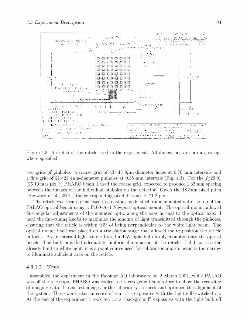
4.3 Experiment Description 94
Figure 4.3: A sketch of the reticle used in the experiment. All dimensions are in mm, exceptwhere specified.
two grids of pinholes: a coarse grid of 43×43 8µm-diameter holes at 0.70 mm intervals anda fine grid of 21×21 4µm-diameter pinholes at 0.35 mm intervals (Fig. 4.3). For the f/29.91(25.10 mas pix−1) PHARO beam, I used the coarse grid, expected to produce 1.32 mm spacingbetween the images of the individual pinholes on the detector. Given the 18.5µm pixel pitch(Hayward et al., 2001), the corresponding pixel distance is 71.2 pix.
The reticle was securely enclosed in a custom-made steel frame mounted onto the top of thePALAO optical bench using a P100–A–1 Newport optical mount. The optical mount allowedfine angular adjustments of the mounted optic along the axes normal to the optical axis. Iused the fine-tuning knobs to maximize the amount of light transmitted through the pinholes,ensuring that the reticle is within 0.5 of being perpendicular to the white light beam. Theoptical mount itself was placed on a translation stage that allowed me to position the reticlein focus. As an internal light source I used a 4 W light bulb firmly mounted onto the opticalbench. The bulb provided adequately uniform illumination of the reticle. I did not use thealready built-in white light: it is a point source used for calibration and its beam is too narrowto illuminate sufficient area on the reticle.
4.3.1.2 Tests
I assembled the experiment in the Palomar AO laboratory on 2 March 2004, while PALAOwas off the telescope. PHARO was cooled to its cryogenic temperature to allow the recordingof imaging data. I took test images in the laboratory to check and optimize the alignment ofthe system. These were taken in series of ten 1.4 s exposures with the lightbulb switched on.At the end of the experiment I took ten 1.4 s “background” exposures with the light bulb off
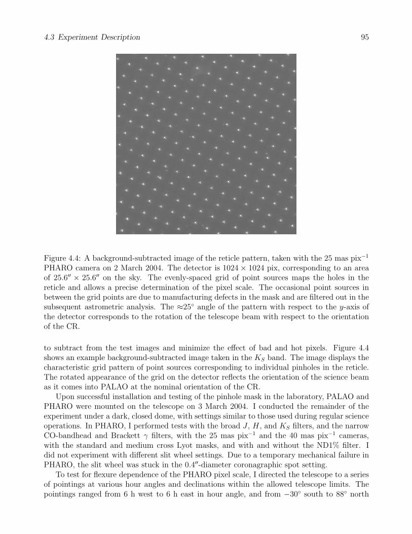
4.3 Experiment Description 95
Figure 4.4: A background-subtracted image of the reticle pattern, taken with the 25 mas pix−1
PHARO camera on 2 March 2004. The detector is 1024 × 1024 pix, corresponding to an areaof 25.6′′ × 25.6′′ on the sky. The evenly-spaced grid of point sources maps the holes in thereticle and allows a precise determination of the pixel scale. The occasional point sources inbetween the grid points are due to manufacturing defects in the mask and are filtered out in thesubsequent astrometric analysis. The ≈25 angle of the pattern with respect to the y-axis ofthe detector corresponds to the rotation of the telescope beam with respect to the orientationof the CR.
to subtract from the test images and minimize the effect of bad and hot pixels. Figure 4.4shows an example background-subtracted image taken in the KS band. The image displays thecharacteristic grid pattern of point sources corresponding to individual pinholes in the reticle.The rotated appearance of the grid on the detector reflects the orientation of the science beamas it comes into PALAO at the nominal orientation of the CR.
Upon successful installation and testing of the pinhole mask in the laboratory, PALAO andPHARO were mounted on the telescope on 3 March 2004. I conducted the remainder of theexperiment under a dark, closed dome, with settings similar to those used during regular scienceoperations. In PHARO, I performed tests with the broad J , H , and KS filters, and the narrowCO-bandhead and Brackett γ filters, with the 25 mas pix−1 and the 40 mas pix−1 cameras,with the standard and medium cross Lyot masks, and with and without the ND1% filter. Idid not experiment with different slit wheel settings. Due to a temporary mechanical failure inPHARO, the slit wheel was stuck in the 0.4′′-diameter coronagraphic spot setting.
To test for flexure dependence of the PHARO pixel scale, I directed the telescope to a seriesof pointings at various hour angles and declinations within the allowed telescope limits. Thepointings ranged from 6 h west to 6 h east in hour angle, and from −30 south to 88 north

4.3 Experiment Description 96
in declination, at steps of 1.5 h in hour angle and 15 in declination. During most of theexperiment, the CR rotator angle was maintained near 333.5, placing the y-axis on PHAROwithin ≈1.5 of north. Limited experiments with rotating the CR in steps of 90 were alsoperformed at zenith and at −30 declination on the meridian. For the flexure test I employedthe KS filter in PHARO, which is the one used in most scientific AO observations with the200′′ and allows fine sampling of the 90 mas (FWHM) diffraction-limited PALAO PSF withthe 25 mas pix−1 camera. The remaining wheel settings for the flexure experiment were: “0.4′′
coronagraph” (slit wheel), “medium cross” (Lyot wheel), and “open” (grism wheel).Throughout the experiment the tip-tilt (TT) and the deformable mirror (DM) loops re-
mained open. Because of the small spacing between the pinholes in the reticle, wave-frontsensing on any particular pinhole would have been complicated by stray light contaminationfrom neighboring holes. Although the practice of leaving the TT and DM off is in contrast withnormal science operations, it was not expected to affect the final result. Changes in the detectorpixel scale are expected to be induced by distortions in the geometrical figures (e.g., because ofchanging gravity vectors) of the optics. If the TT and DM mirrors suffer such distortions, theywould be relayed along the beam path regardless of whether their actuators are active (i.e., asin closed loop operation) or not.
4.3.1.3 Astrometric Measurements
A total of 450 PHARO images were taken during the course of the experiment. The pixelcoordinates of the evenly-spaced points sources in each of the images were measured with anautomated procedure to fit Gaussian profiles. The width of the Gaussian profiles was set tomatch the PSF FWHM: 3.4 pix atKS and Brackett γ, 2.6 pix atH and 2.1 pix at J . Extraneoussources in between the grid points were ignored, as they were caused by manufacturing defectsin the reticle substrate. Point sources near the coronagraphic spot or near bad pixels on thedetector were also removed from the subsequent analysis. Given the spot brightness and shapeof the PSF, the spot coordinates were obtained to a mean precision of ±0.026 pix in x and±0.030 pix in y.
I calculated the distances between each spot and its closest neighbors on the grid to lookfor variation with detector position. Figure 4.5 shows the obtained inter-spot distances alongthe two grid axes for a case in which the telescope was pointed at zenith, and the CR anglewas set to 333.5. Circles mark distance measurements in the direction of the continuous-linevector, and squares mark measurements along the dashed-line vector. Each point is located inthe middle of two neighboring grid spots (not shown) and its size is linearly proportional to thedistance between the spots. The shortest and the longest inter-spot pixel distance along eachdirection is labeled above the corresponding dot. The lack of data near (x, y) = (340, 230) iscaused by an area of bad pixels on the detector.
It is immediately evident from Figure 4.5 that the pixel scale across the array is not uniform.Along the position angle (PA) of the continuous-line vector the inter-spot distance is smallest(71.65 pix) in the top left corner of the array and largest (72.38 pix) in the bottom right corner.The variation of the pixel scale along the PA of the dashed-line vector follows an approximatelyvertical direction, with the shortest inter-spot distance (72.25 pix) near the bottom left cornerof the array and the longest (72.73 pix) near the top.
To first order, the measurements of the inter-spot distances point to a tilt in the opticalsystem. Indeed, the plane of the PHARO detector is known to be tilted by 0.1 with respect

4.3 Experiment Description 97
Figure 4.5: Pixel distances between neighboring grid spots in the reticle image. Circles denotedistances along the continuous-line vector, and squares mark distances along the dashed-linevector. Each point is located in the middle of two neighboring grid spots (not shown), andits diameter is linearly proportional to the distance between the spots. The minimum andmaximum inter-spot pixel distances along each direction are marked above the correspondingpoint.

4.3 Experiment Description 98
to the f/29.91 focal plane by design. In §4.4.1 I will also discuss probable apparent beam tiltthat was induced by my imperfect alignment of the reticle perpendicularly to the beam. Afurther comparison with the expected inter-spot pixel distance of 71.2 pix also reveals possibledirection-dependent magnification. Both effects, tilt and magnification, are typical of focalplane distortion patterns, such as pincushion or barrel.
4.3.2 Binary Stars
Binary stars and various rich stellar fields are secondary astrometric calibrators. Accuratepositions of each of the stars in the field need to have been established a priori with the use ofa primary astrometric calibrator. Such measurements are available in the literature, and I haveused binary stars with well-characterized orbital solutions from the Sixth Catalog of Orbits ofVisual Binary Stars (Hartkopf & Mason, 2005). Binary star observations can be performedin identical manner to science observations, and therefore astrometric measurements based onbinary stars do not suffer from the non-common path errors associated with the use of thepinhole mask described in §4.3.1.
4.3.2.1 Observations
Observations of binaries for pixel scale calibration were conducted on most observing runs duringthe course of my three-year survey for sub-stellar companions to young solar analogs (Metchev& Hillenbrand, 2004). The binaries were selected from the subset of “calibration candidates”recommended by Hartkopf & Mason (2003). These have either well-known “grade 1” orbits,with minimal uncertainties of the orbital elements, or less well-known (grade 4–5) orbits withlong orbital periods (&1000 yr), resulting in negligible systematic errors in the predicted binaryconfiguration over tens of years. The list of the calibration binaries that I have used, alongwith their relevant orbital parameters, is given in Table 4.1. All binary systems in the Tableare named using their Washington Double Star (WDS) Catalog (Mason et al., 2001) identifiers.
Table 4.2 gives the dates on which each calibration binary was observed and details thetelescope orientation during each observation. The calibration observations were conductedunder a broad range of atmospheric conditions, from calm and clear to windy and with heavycirrus. The natural seeing varied from 0.5′′–2′′ at KS band, and the airmass between 1.0 and2.0. The AO loop rate for these bright (V = 3 − 6 mag) stars was set between 500 Hz and1500 Hz. The Strehl ratios were estimated to be between 10% and 70%, sometimes varying on atimescale of minutes. All binaries were observed with the H , KS, or Brγ filters in PHARO withan ND 0.1% or ND 1.0% filter inserted in front of the array to keep the stars from saturatingin the shortest (1.4 s) exposures.
Because of unstable atmospheric conditions, the AO correction was sometimes inadequate,resulting in isolated poor (not diffraction-limited) images. Less often, entire sequences of ob-servations were of low quality, such as those of WDS 18055 + 0230 on 5 February 2004 and 27June 2004 (Table 4.2). Poor images were excluded from the subsequent analysis, for which Ihave chosen only images in which a diffraction-limited core of FWHM = 3.6–4.0 pix was clearlyvisible.

4.3E
xperim
ent
Descrip
tion99
Table 4.1: Observed Calibration Binaries and Parameters of Their Relative Orbits
Binary a P T0 e i Ω ω WDS Ref.(WDS) (arcsec) (years) (year) (degrees) (degrees) (degrees) (degree) grade09006+4147 0.6472 ± 0.0010 21.776 ± 0.017 1993.725 ± 0.023 0.1507 ± 0.0008 131.26 ± 0.13 204.39 ± 0.19 32.52 ± 0.36 1 115232+3017 0.8676 ± 0.0012 41.585 ± 0.013 1933.721 ± 0.057 0.2620 ± 0.0031 59.03 ± 0.15 203.19 ± 0.20 38.42 ± 0.51 1 216147+3352 5.927 888.989 1826.949 0.7605 31.795 16.889 72.201 4 318055+0230 4.5540 ± 0.0052 88.38 ± 0.02 1895.94 ± 0.02 0.4992 ± 0.0004 121.16 ± 0.08 302.12 ± 0.10 14.0 ± 0.1 1 420467+1607 10.22 3249 2305 0.88 148.78 88.06 331.16 4 523052−0742 0.2026 ± 0.0007 21.840 ± 0.019 1983.108 ± 0.022 0.3878 ± 0.0025 48.01 ± 0.042 204.87 ± 0.50 82.83 ± 0.45 1 123322+0705 0.173 30.73 1987.47 0.263 31.0 126.8 57.0 1 6
References.—1. Hartkopf et al. (1996); 2. Mason et al. (1999); 3. Scardia (1979); 4. Pourbaix (2000); 5. Hale (1994); 6. Hartkopf & Mason (2000).
Notes.—Explanation of orbital parameters: a—semi-major axis; P—period; T0—epoch of periastron; e—eccentricity; i—inclination; Ω—longitude of periastron; ω—longitude of
the ascending node.

4.3E
xperim
ent
Descrip
tion100
Table 4.2: Observations of Calibration BinariesDate Epoch Binary Ephemerides CR Angle Hour Angle DEC Note(UT) (year) (WDS) ρ(′′) P.A.() (degrees) (degrees) (degrees)Jun 23, 2002 2002.476 18055+0230 4.3351 142.8677 63.5 · · · 2.50May 10, 2003 2003.356 09006+4147 0.7219 13.0340 63.5 34.0 – 37.9 W 41.78May 11, 2003 2003.359 20467+1607 9.2023 265.7002 243.5 19.9 – 17.5 E 16.12Jul 15, 2003 2003.537 16147+3352 7.0780 236.4879 63.5, 153.5, 243.5, 333.5 11.9 – 49.0 W 33.86Jul 16, 2003 2003.539 18055+0230 4.5697 140.8363 63.5, 153.5, 243.5, 333.5 5.3 E – 15.7 W 2.50Sep 20, 2003 2003.720 23322+0705 0.1936 6.3602 63.5, 333.5 15.0 – 32.5 W 7.08Sep 21, 2003 2003.723 18055+0230 4.6168 140.4406 63.5 16.4 – 18.8 2.50
23052–0742 0.1223 230.8686 63.5 19.0 – 15.0 E −7.70Dec 9, 2003 2003.939 09006+4147 0.7072 7.8751 243.2 39.8 – 41.3 W 41.78Feb 5, 2004 2004.099 09006+4147 0.7018 6.4283 243.5, 333.5 11.6 – 16.2 W 41.78
18055+0230 4.6881 139.8472 333.5 48.3 – 45.9 E 2.50 poorFeb 6, 2004 2004.101 09006+4147 0.7018 6.4104 333.5 15.5 – 21.5 W 41.78
18055+0230 4.6885 139.8438 333.5 41.4 – 39.1 E 2.50Feb 7, 2004 2004.104 18055+0230 4.6891 139.8386 333.5 38.3 – 35.1 E 2.50Jun 26, 2004 2004.486 18055+0230 4.7681 139.1897 62.9, 152.9, 242.9, 332.9 9.6 – 15.6 W 2.50
20467+1607 9.1805 265.6374 152.9 25.4 – 26.5 W 16.12Jun 27, 2004 2004.489 18055+0230 4.7685 139.1864 152.9 66.6 – 66.9 W 2.50 poor
20467+1607 9.1805 265.6373 152.9 29.0 – 29.4 W 16.12Jun 28, 2004 2004.491 15232+3017 0.5092 105.0731 152.9 3.8 – 5.5 W 30.29
16147+3352 7.0953 236.6373 152.9 6.4 – 6.0 E 33.8618055+0230 4.7689 139.1832 62.9 25.9 – 26.2 W 2.50
Oct 4, 2004 2004.759 09006+4147 0.6744 0.1452 332.9 39.4 – 38.5 E 41.78Oct 5, 2004 2004.762 18055+0230 4.8243 138.7337 242.9, 332.9 21.2 – 23.3 W 2.50
20467+1607 9.1751 265.6219 242.9, 332.9 15.1 – 13.1 E 16.12

4.3 Experiment Description 101
B
A
EN
CR angle = 63.5 deg
B
A
E
N
CR angle = 333.5 deg
B
A
EN
CR angle = 243.5 deg
B
A
EN
CR angle = 153.5 deg
Figure 4.6: Images of the calibration binary WDS 16147+3352 taken in the KS band on 15July 2003 at four mutually orthogonal orientations of the CR rotator. The binary separationon that date was predicted to be 7.0780′′ and the position angle 236.4879.
4.3.2.2 Tests
Each binary star was dithered to the center and vertices of a 6′′ on a side box dither pattern forthe purpose of sky-subtraction. The five-point dither patterns were performed generally nearthe center of the array to allow quick comparison among different binaries and observing runs.On the nights of 15 and 16 July 2003 I performed extensive tests of the variation of the pixelscale across the entire PHARO array at four orthogonal orientations of the CR rotator: 333.5—N-up, E-left (nominal); 63.5—N-left, E-down; 153.5—N-down, E-right; and 243.5—N-right,E-up (Fig. 4.6).
4.3.2.3 Astrometric Measurements
The pixel coordinates of the binary star components were obtained in a manner similar tothe point source coordinates in the reticle experiment (§4.3.1.3). I fitted Gaussian profiles to

4.3 Experiment Description 102
Figure 4.7: Positional and CR dependence of the pixel scale of PHARO based on observa-tions of the WDS 16147+3352 calibration binary on 15 July 2003. The dot size indicates thepixel scale, decreasing linearly from the largest value (25.54 mas pix−1) to the smallest one(25.19 mas pix−1). The arrow hands point to north and east, with East being 90 counter-clockwise from north. The binary orientation in each panel is the same as in the correspondingpanel of Fig. 4.6.
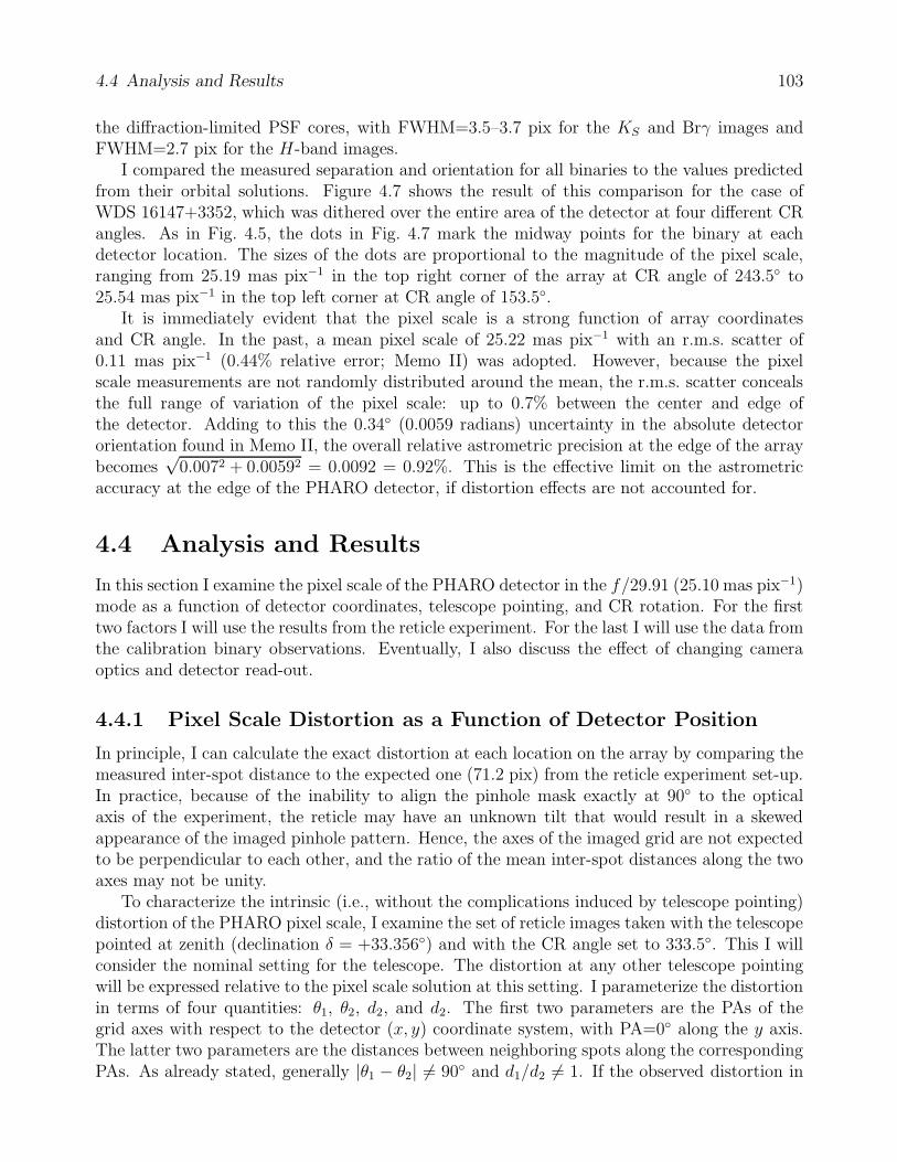
4.4 Analysis and Results 103
the diffraction-limited PSF cores, with FWHM=3.5–3.7 pix for the KS and Brγ images andFWHM=2.7 pix for the H-band images.
I compared the measured separation and orientation for all binaries to the values predictedfrom their orbital solutions. Figure 4.7 shows the result of this comparison for the case ofWDS 16147+3352, which was dithered over the entire area of the detector at four different CRangles. As in Fig. 4.5, the dots in Fig. 4.7 mark the midway points for the binary at eachdetector location. The sizes of the dots are proportional to the magnitude of the pixel scale,ranging from 25.19 mas pix−1 in the top right corner of the array at CR angle of 243.5 to25.54 mas pix−1 in the top left corner at CR angle of 153.5.
It is immediately evident that the pixel scale is a strong function of array coordinatesand CR angle. In the past, a mean pixel scale of 25.22 mas pix−1 with an r.m.s. scatter of0.11 mas pix−1 (0.44% relative error; Memo II) was adopted. However, because the pixelscale measurements are not randomly distributed around the mean, the r.m.s. scatter concealsthe full range of variation of the pixel scale: up to 0.7% between the center and edge ofthe detector. Adding to this the 0.34 (0.0059 radians) uncertainty in the absolute detectororientation found in Memo II, the overall relative astrometric precision at the edge of the arraybecomes
√0.0072 + 0.00592 = 0.0092 = 0.92%. This is the effective limit on the astrometric
accuracy at the edge of the PHARO detector, if distortion effects are not accounted for.
4.4 Analysis and Results
In this section I examine the pixel scale of the PHARO detector in the f/29.91 (25.10 mas pix−1)mode as a function of detector coordinates, telescope pointing, and CR rotation. For the firsttwo factors I will use the results from the reticle experiment. For the last I will use the data fromthe calibration binary observations. Eventually, I also discuss the effect of changing cameraoptics and detector read-out.
4.4.1 Pixel Scale Distortion as a Function of Detector Position
In principle, I can calculate the exact distortion at each location on the array by comparing themeasured inter-spot distance to the expected one (71.2 pix) from the reticle experiment set-up.In practice, because of the inability to align the pinhole mask exactly at 90 to the opticalaxis of the experiment, the reticle may have an unknown tilt that would result in a skewedappearance of the imaged pinhole pattern. Hence, the axes of the imaged grid are not expectedto be perpendicular to each other, and the ratio of the mean inter-spot distances along the twoaxes may not be unity.
To characterize the intrinsic (i.e., without the complications induced by telescope pointing)distortion of the PHARO pixel scale, I examine the set of reticle images taken with the telescopepointed at zenith (declination δ = +33.356) and with the CR angle set to 333.5. This I willconsider the nominal setting for the telescope. The distortion at any other telescope pointingwill be expressed relative to the pixel scale solution at this setting. I parameterize the distortionin terms of four quantities: θ1, θ2, d2, and d2. The first two parameters are the PAs of thegrid axes with respect to the detector (x, y) coordinate system, with PA=0 along the y axis.The latter two parameters are the distances between neighboring spots along the correspondingPAs. As already stated, generally |θ1 − θ2| 6= 90 and d1/d2 6= 1. If the observed distortion in

4.4 Analysis and Results 104
the reticle images was caused only by reticle and detector tilt, θ1, θ2, d1, and d2 would attainconstant values regardless of detector position. Higher-order image distortion will induce x-and y-dependent variation of these parameters.
I fit for the measured angles and spacings (Fig. 4.5) between neighboring grid points alongboth grid axes, using first-degree linear two-dimensional (2D) polynomials for the angles andfor the inter-spot distances. At the center (512,512) of the array, I obtain:
θ1(512, 512) = 64.8455 ± 0.0025
θ2(512, 512) = 155.0740 ± 0.0051
d1(512, 512) = 72.0099 ± 0.0051 pix
d2(512, 512) = 72.4521 ± 0.0068 pix.
The errors represent the r.m.s. scatter of 15 independent measurements and fits.Assuming that the image distortion vanishes at the center of the array in the nominal
telescope setting, I use d1 and d2 as two separate unit vectors (with directions along θ1 and θ2,and lengths d1 and d2, respectively) to measure the pixel scale along either direction relativeto the center of the array. Without being able to change the orientation of the reticle imageon the array, the lengths of the two unit vectors cannot be compared. However, an absolutedetermination of the pixel scale will be possible when I consider binary star images taken atmutually perpendicular CR angles in §4.4.3.
I create an array of the expected spot positions, provided that tip and tilt are the onlydistortions in the beam, i.e., assuming that each spot is an integer number of d1 and d2 vectorlengths away from the spot nearest the detector center. The coordinate residuals between theactual and the expected spot positions reveal the intrinsic pixel scale distortion of the PHAROf/29.91 beam. Panels (a) and (b) of Figure 4.8 show the direction and the magnitude of thedistortion. Letting (x′, y′) be the distortion-corrected pixel coordinates, I find that the intrinsicpixel scale distortion is well fit by the following polynomials:
x′(xc, yc) = 512 + a0 + a1yc + a2y2c + a3xc + a4xcyc + a5x
2c (4.1)
y′(xc, yc) = 512 + b0 + b1yc + b2xc, (4.2)
where xc = x − 512 and yc = y − 512. The values of the individual parameters are tabulatedin Table 4.3. The reduced χ2 values of the fits for each of the 15 reticle images taken at thenominal telescope setting vary from 0.74 to 1.01 for x′ and from 0.54 to 1.54 for y′. There isthus no need for xcyc cross-term dependence in either x′ or y′.
Expressions 4.1 and 4.2 with the parameter values tabulated in Table 4.3 describe theintrinsic pixel scale distortion of the PHARO 25 mas pix−1 camera when the telescope is pointedat zenith.
4.4.2 Pixel Scale Variation with Hour Angle and Declination
Having established the intrinsic PHARO distortion, I pursue a more general solution of the pixelscale for arbitrary telescope hour angle and declination, though still at a fixed CR angle. Be-cause of limited experimentation with varying the CR angle during the reticle experiment, theseobservations had insufficient phase-space coverage to characterize its effect on the pixel scale.Nevertheless, CR-angle dependent variations were measured from the binary star observations
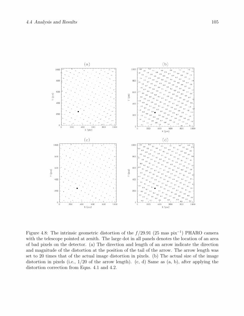
4.4 Analysis and Results 105
Figure 4.8: The intrinsic geometric distortion of the f/29.91 (25 mas pix−1) PHARO camerawith the telescope pointed at zenith. The large dot in all panels denotes the location of an areaof bad pixels on the detector. (a) The direction and length of an arrow indicate the directionand magnitude of the distortion at the position of the tail of the arrow. The arrow length wasset to 20 times that of the actual image distortion in pixels. (b) The actual size of the imagedistortion in pixels (i.e., 1/20 of the arrow length). (c, d) Same as (a, b), after applying thedistortion correction from Eqns. 4.1 and 4.2.
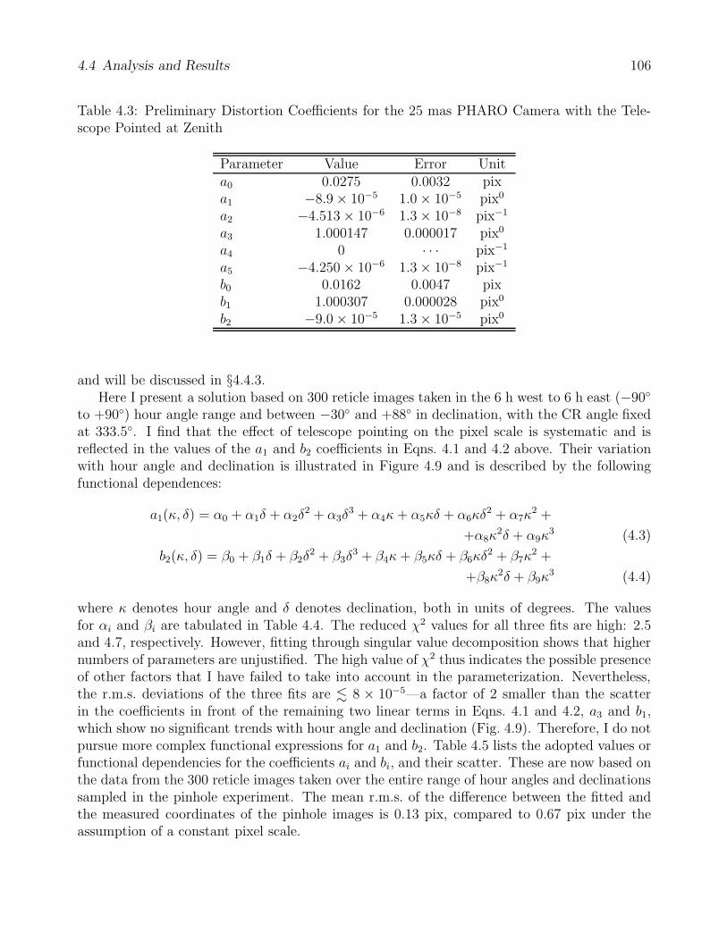
4.4 Analysis and Results 106
Table 4.3: Preliminary Distortion Coefficients for the 25 mas PHARO Camera with the Tele-scope Pointed at Zenith
Parameter Value Error Unita0 0.0275 0.0032 pixa1 −8.9 × 10⁻⁵ 1.0 × 10−5 pix0
a2 −4.513 × 10⁻⁶ 1.3 × 10⁻⁸ pix−1
a3 1.000147 0.000017 pix0
a4 0 · · · pix−1
a5 −4.250 × 10⁻⁶ 1.3 × 10⁻⁸ pix−1
b0 0.0162 0.0047 pixb1 1.000307 0.000028 pix0
b2 −9.0 × 10⁻⁵ 1.3 × 10−5 pix0
and will be discussed in §4.4.3.Here I present a solution based on 300 reticle images taken in the 6 h west to 6 h east (−90
to +90) hour angle range and between −30 and +88 in declination, with the CR angle fixedat 333.5. I find that the effect of telescope pointing on the pixel scale is systematic and isreflected in the values of the a1 and b2 coefficients in Eqns. 4.1 and 4.2 above. Their variationwith hour angle and declination is illustrated in Figure 4.9 and is described by the followingfunctional dependences:
a1(κ, δ) = α0 + α1δ + α2δ2 + α3δ
3 + α4κ+ α5κδ + α6κδ2 + α7κ
2 +
+α8κ2δ + α9κ
3 (4.3)
b2(κ, δ) = β0 + β1δ + β2δ2 + β3δ
3 + β4κ+ β5κδ + β6κδ2 + β7κ
2 +
+β8κ2δ + β9κ
3 (4.4)
where κ denotes hour angle and δ denotes declination, both in units of degrees. The valuesfor αi and βi are tabulated in Table 4.4. The reduced χ2 values for all three fits are high: 2.5and 4.7, respectively. However, fitting through singular value decomposition shows that highernumbers of parameters are unjustified. The high value of χ2 thus indicates the possible presenceof other factors that I have failed to take into account in the parameterization. Nevertheless,the r.m.s. deviations of the three fits are . 8 × 10⁻⁵—a factor of 2 smaller than the scatterin the coefficients in front of the remaining two linear terms in Eqns. 4.1 and 4.2, a3 and b1,which show no significant trends with hour angle and declination (Fig. 4.9). Therefore, I do notpursue more complex functional expressions for a1 and b2. Table 4.5 lists the adopted values orfunctional dependencies for the coefficients ai and bi, and their scatter. These are now based onthe data from the 300 reticle images taken over the entire range of hour angles and declinationssampled in the pinhole experiment. The mean r.m.s. of the difference between the fitted andthe measured coordinates of the pinhole images is 0.13 pix, compared to 0.67 pix under theassumption of a constant pixel scale.

4.4 Analysis and Results 107
Figure 4.9: Third-degree 2D polynomial fits to the dependence of the linear expansion coeffi-cients in Eqns. 4.1 and 4.2 on hour angle (west is negative, east is positive) and declination.The contour spacing is 0.0001 pix pix−1. Coefficients a1 and b2 show significant variation, whilethe variation of a3 and b1 is negligible. The −0.0006 and −0.0007 contour levels in the bottomright corner of the top left panel are artifacts due to the polynomial fitting of the data: nomeasurements were taken at this extreme (and unattainable) combination of hour angle anddeclination.

4.4 Analysis and Results 108
Table 4.4: Coefficients in the Expansions of a1 (Eqn. 4.3) and b2 (Eqn. 4.4)
Parameter Value Error Unitα0 −2.496 × 10⁻⁴ 5.4 × 10⁻⁶ degree0
α1 7.22 × 10⁻⁶ 1.5 × 10⁻⁷ degree−1
α2 9.16 × 10⁻⁸ 6.5 × 10⁻⁹ degree−2
α3 −5.47 × 10⁻¹⁰ 6.5 × 10⁻¹¹ degree−3
α4 −8.14 × 10⁻⁶ 1.1 × 10⁻⁷ degree−1
α5 0 · · · degree−2
α6 0 · · · degree−3
α7 2.14 × 10⁻⁸ 1.7 × 10⁻⁹ degree−2
α8 −1.031 × 10⁻⁹ 3.1 × 10⁻¹¹ degree−3
α9 3.66 × 10⁻¹⁰ 1.7 × 10⁻¹¹ degree−3
β0 1.997 × 10⁻⁴ 5.3 × 10⁻⁶ degree0
β1 −1.054 × 10⁻⁵ 1.5 × 10⁻⁷ degree−1
β2 −7.41 × 10⁻⁸ 6.4 × 10⁻⁹ degree−2
β3 5.37 × 10⁻¹⁰ 6.4 × 10⁻¹¹ degree−3
β4 7.58 × 10⁻⁶ 1.0 × 10⁻⁷ degree−1
β5 0 · · · degree−2
β6 0 · · · degree−3
β7 1.07 × 10⁻⁸ 1.7 × 10⁻⁹ degree−2
β8 8.87 × 10⁻¹⁰ 3.1 × 10⁻¹¹ degree−3
β9 −2.83 × 10⁻¹⁰ 1.7 × 10⁻¹¹ degree−3
Table 4.5: Final Distortion Coefficients and Expressions at Arbitrary Telescope Hour Angleand Declination
Coefficient Value or Equation R.M.S. Scatter Unita0 0.018 0.035 pixa1 Eqn. 4.3 6.8 × 10−5 pix0
a2 −4.51 × 10⁻⁶ 1.1 × 10⁻⁷ pix−1
a3 0.99983 1.7 × 10−4 pix0
a4 0 · · · pix−1
a5 −4.37 × 10⁻⁶ 1.2 × 10⁻⁷ pix−1
b0 0.019 0.046 pixb1 1.00001 1.4 × 10−4 pix0
b2 Eqn. 4.4 8.5 × 10−5 pix0
4.4 Analysis and Results 109
4.4.3 Absolute Calibration of the Pixel Scale Distortion
The parametric fit derived in §4.4.1 and §4.4.2 is based on data from an internal light source andis incomplete because of unknown beam tilt. The pixel scale distortion is known only modulo theratio of the lengths of the d1 and d2 unit vectors. Because the mounting of the astrometric maskdid not allow for rotation along the beam axis, I could not sample the pixel scale with differentreticle orientations to determine the beam tilt. Here I have used observations of binary starsat different CR angles to determine this tilt and to transform the partially distortion-correctedpixel coordinates (x′, y′) (Eqns. 4.1 and 4.2) to a fully distortion-corrected coordinate system(x′′, y′′).
4.4.3.1 Additional Parameterization: Beam Tilt
In principle, the reticle beam tilt can be readily calculated from the values of θ1, θ2, d1, andd2, obtained during the reticle experiment (§4.4.2). However, because of the non-common pathbetween the reticle and the science beams (Fig. 4.2), the reticle beam tilt will, in general,be different from the tilt of the science beam. I will therefore proceed with an independentparameterization of the science beam tilt. The higher-order distortion of the science beammay also be different from that of the reticle beam (described by Eqns. 4.1–4.4). However,the binary star observations will show (§4.4.4) that the high-order parameterization obtainedfrom the reticle experiment is adequate for the science beam. This implies that most of thehigh-order distortion in the science beam arises in PALAO and PHARO, after the primary andsecondary telescope mirrors, in agreement with the larger number of optics at that point in theoptical train.
A tilted plane can be parameterized by two angle variables in the detector coordinate system:one, ζ , to specify the tilt between the two planes, and another, φ, to specify the orientationof their intersection (a line). Figure 4.10 demonstrates this parameterization for the detector(x′, y′) and tilted beam (xb, yb) planes, which intersect along the line AB. The projection (xt, yt)of the (xb, yb) coordinate system on the detector is a suitable one to use for images of the sky,since the xt and yt axes are orthogonal. The projections of any other pairs of orthonormal (xb, yb)axes, where neither of the vectors xb or yb lie along AB, would not be mutually orthogonaland would require an extra parameter for their description.
Because the xt and yt unit vectors do not have the same length (xb and yb do), distancesalong the xt direction will be magnified by |xt|/|yt| = 1/ cos ζ with respect to distances alongthe yt direction. Furthermore, a 90 rotation of a vector in the telescope beam plane (xt, yt;e.g., via a CR rotation) will, in general, result in a 90 + ε rotation of the projection of thevector on the detector. For small values of ζ , −ζ2/4 ≤ ε ≤ ζ2/4. This is precisely the effectthat limited the absolute determination of the plate scale in §4.4.2. By taking images of a singlebinary star at two different orientations of the CR, from the two independent measurementsof the binary separation and position angle, I can determine the direction φ of the tilt and themagnification factor 1/ cos ζ . I was unable to do this with the reticle because the orientationof the reticle beam was fixed with respect to the detector.
To this end, I transform the detector (x′, y′) coordinates of each of the binary components tothe (xt, yt) coordinate system, apply a magnification of 1/ cos ζ along the yt axis, and transformback to the detector system. The final coordinates (x′′, y′′), obtained in this manner, are thefully distortion-corrected pixel coordinates. Using the center of the detector (512,512) as the

4.4 Analysis and Results 110
Figure 4.10: A diagram of the intersection between the detector image plane (x′, y′) and thetilted beam plane (xb, yb). The two planes intersect along the line AB at an angle ζ . Theorientation of AB with respect to the detector x axis in the image plane is φ. The projectionsof the xb and yb unit vectors onto the image plane are denoted as xt and yt. Right angles aremarked with square corners.
origin, the exact coordinate transformations are:
(
xtyt
)
=
(
cosφ sin φ
− sinφcos ζ
cos φcos ζ
)(
x′ − 512y′ − 512
)
(4.5)
(
x′′
y′′
)
=
(
cosφ − sinφsinφ cosφ
)(
xtyt
)
+
(
512512
)
. (4.6)
Therefore:
(
x′′
y′′
)
=
(
sin2 φcos ζ
+ cos2 φ sin φ cosφ− sinφ cosφcos ζ
sin φ cosφ− sinφ cosφcos ζ
sin2 φ+ cos2 φcos ζ
)
(
x′ − 512y′ − 512
)
+
+
(
512512
)
. (4.7)
4.4.3.2 Solving for the Beam Tilt
I solved Eqn. 4.7 using observations of the calibration binaries WDS 16147+3352 and WDS18055+0230 taken at four orthogonal CR orientations: 333.5 (nominal), 63.5, 153.5, and243.5. Detailed observations of these two binaries were conducted on July 15 and 16 2003(Table 4.2), where the binaries were dithered over the entire array at each CR angle, with thepurpose of mapping the pixel scale distortion. Because of the 90 step between CR orientations,the final distortion-corrected coordinates x′′ and y′′ should map onto each other from one CRorientation to the next. That is,
∆x′′333.5 = ∆y′′63.5 = ∆x′′153.5 = ∆y′′243.5 (4.8)
∆y′′333.5 = ∆x′′63.5 = ∆y′′153.5 = ∆x′′243.5, (4.9)

4.4 Analysis and Results 111
where ∆x′′ψ and ∆y′′ψ are the x′′ and y′′ components of the distortion-corrected binary separationat a CR angle of ψ. Eqns. 4.8 and 4.9 can be solved for each pair of mutually perpendicular CRorientations, yielding four distinct solutions per binary star for the orientation φ of the beamtilt and for the magnification factor 1/ cos ζ . Combining the results for the two binaries, I find
φ = 83.3 ± 2.5 (4.10)1
cos ζ= 1.0069 ± 0.0006, (4.11)
where the uncertainties represent the r.m.s. scatter of the 8 solutions. The beam tilt angle isthus ζ = 6.7. This is too large compared to the 0.1 detector tilt from the PHARO designspecifications. It is also unrelated to the possible tilt of the reticle beam because the reticleis not in the science beam. The observed science beam tilt may be due to the fact that thedetector is likely offset from the center of the focal plane, in which case the dominant term ofthe pincushion or of the barrel distortion may be tilt.
After adding beam tilt, parameterized by φ and 1/ cos ζ to the overall distortion correction,the astrometric measurements of the calibration binaries become randomly distributed aroundthe mean value and have their r.m.s. scatter reduced by a factor of 4. Figure 4.11 shows theimprovement in the pixel scale uniformity, as calculated using WDS 16147+3352 after applyingthe full distortion correction. For this calibration binary, the astrometric precision was 0.44%(r.m.s.) without applying any beam tilt or distortion tilt correction (Fig. 4.7). The r.m.s. scatterimproves to 0.25% after applying the beam tilt correction and further decreases to 0.11% afterapplying both the beam tilt and the higher-order distortion correction. The largest astrometricr.m.s. scatter, 0.15%, is observed in the case of the binary WDS 18055+0230. This I set as theoverall limit on the precision with the PHARO 25 mas pix−1 camera.
4.4.3.3 Complete Characterization of the Detector Distortion
The complete distortion solution for the 25 mas pix−1 PHARO pixel scale is thus based onEqns. 4.1–4.4 and 4.7–4.11, with the relevant polynomial coefficients tabulated in Tables 4.4 and4.5. A suite of IDL programs that corrects the PHARO distortion using these mathematical rela-tions can be found at http://www.astro.caltech.edu/∼metchev/AO/PHARO 25mas distortion/.
Figure 4.12 illustrates the total amount of distortion (arrows) present on the array withthe telescope pointed at zenith and the CR rotator at two mutually perpendicular orientations:333.5 (nominal; panels a, b) and 63.5 (panels c, d). The dashed lines in Fig. 4.12a,c indicatethe high-order distortion component only. In the case of the nominal CR setting, the dashedlines are identical to the arrows in Fig. 4.8a. Figure 4.12 clearly demonstrates that beam tilt isthe dominant source of pixel scale distortion and that it is a strong function of the CR angle.
4.4.4 Absolute Pixel Scale of the 25 mas pix−1 PHARO Camera
Having achieved a quantitative understanding of the distortion of the PHARO camera, I cannow accurately determine its mean pixel scale and orientation with respect to the celestialcompass rose. For the purpose, I use the results from the calibration binary observations. Thederived pixel scale and CR angle CRN at which the detector is aligned with the celestial axes aregiven in Table 4.6. The table lists the individual values for each calibration binary observationat each CR angle, the mean values for each star from all (N) measurements on a given date at
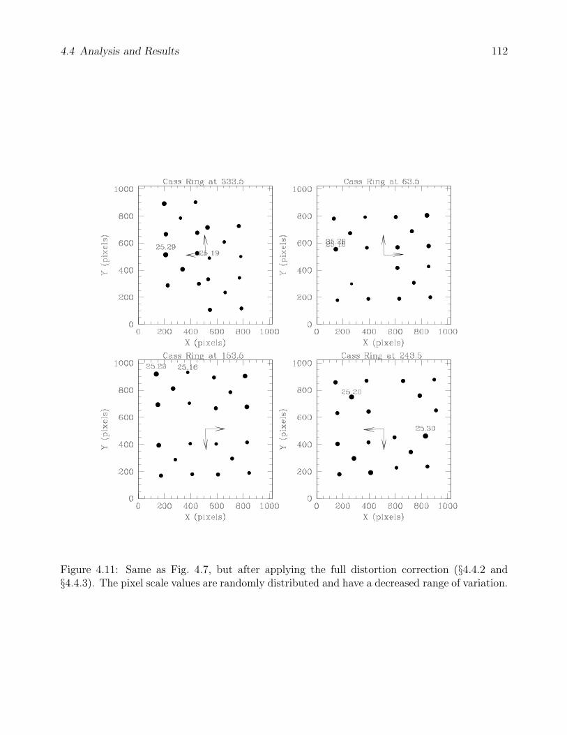
4.4 Analysis and Results 112
Figure 4.11: Same as Fig. 4.7, but after applying the full distortion correction (§4.4.2 and§4.4.3). The pixel scale values are randomly distributed and have a decreased range of variation.

4.4 Analysis and Results 113
Figure 4.12: Distortion of the PHARO 25 mas pix−1 camera with the telescope pointed atzenith and at CR angles of 333.5 (nominal orientation; panels a, b) and 63.5 (c, d). Thearrows in panels (a, c) denote the total distortion, while the dashed lines denote the high-orderdistortion component only. The length of the arrows corresponds to the pixel magnitude of thedistortion (panels c, d) multiplied by a factor of 10. A comparison to a distortion-correctedmap of the array, as in Figure 4.8, is not possible, because a finely-spaced grid of measurementsof the calibration binaries was not obtained. Instead, the accuracy of the distortion correctionis inferred from the small scatter in the pixel scale across the array (Fig. 4.11).
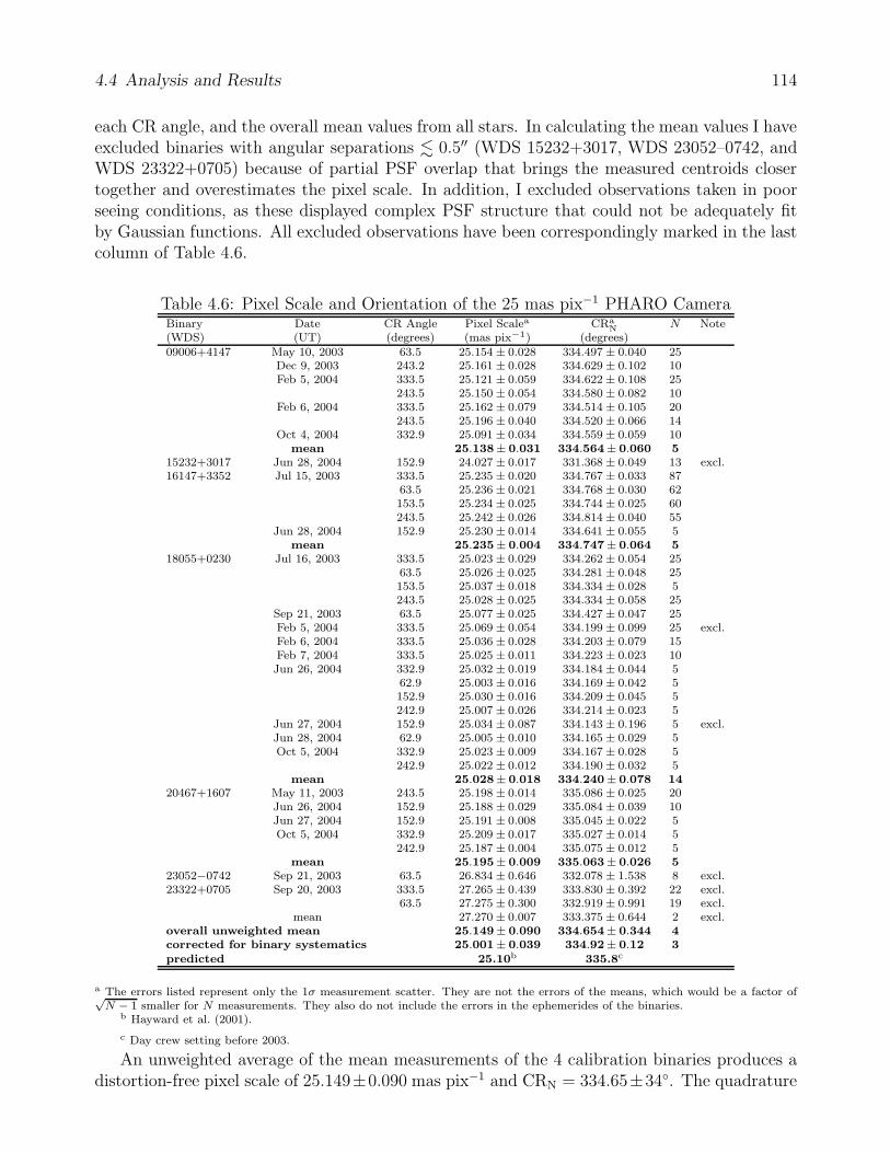
4.4 Analysis and Results 114
each CR angle, and the overall mean values from all stars. In calculating the mean values I haveexcluded binaries with angular separations . 0.5′′ (WDS 15232+3017, WDS 23052–0742, andWDS 23322+0705) because of partial PSF overlap that brings the measured centroids closertogether and overestimates the pixel scale. In addition, I excluded observations taken in poorseeing conditions, as these displayed complex PSF structure that could not be adequately fitby Gaussian functions. All excluded observations have been correspondingly marked in the lastcolumn of Table 4.6.
Table 4.6: Pixel Scale and Orientation of the 25 mas pix−1 PHARO CameraBinary Date CR Angle Pixel Scalea CRa
N N Note(WDS) (UT) (degrees) (mas pix−1) (degrees)09006+4147 May 10, 2003 63.5 25.154 ± 0.028 334.497 ± 0.040 25
Dec 9, 2003 243.2 25.161 ± 0.028 334.629 ± 0.102 10Feb 5, 2004 333.5 25.121 ± 0.059 334.622 ± 0.108 25
243.5 25.150 ± 0.054 334.580 ± 0.082 10Feb 6, 2004 333.5 25.162 ± 0.079 334.514 ± 0.105 20
243.5 25.196 ± 0.040 334.520 ± 0.066 14Oct 4, 2004 332.9 25.091 ± 0.034 334.559 ± 0.059 10
mean 25.138± 0.031 334.564± 0.060 5
15232+3017 Jun 28, 2004 152.9 24.027 ± 0.017 331.368 ± 0.049 13 excl.16147+3352 Jul 15, 2003 333.5 25.235 ± 0.020 334.767 ± 0.033 87
63.5 25.236 ± 0.021 334.768 ± 0.030 62153.5 25.234 ± 0.025 334.744 ± 0.025 60243.5 25.242 ± 0.026 334.814 ± 0.040 55
Jun 28, 2004 152.9 25.230 ± 0.014 334.641 ± 0.055 5mean 25.235± 0.004 334.747± 0.064 5
18055+0230 Jul 16, 2003 333.5 25.023 ± 0.029 334.262 ± 0.054 2563.5 25.026 ± 0.025 334.281 ± 0.048 25153.5 25.037 ± 0.018 334.334 ± 0.028 5243.5 25.028 ± 0.025 334.334 ± 0.058 25
Sep 21, 2003 63.5 25.077 ± 0.025 334.427 ± 0.047 25Feb 5, 2004 333.5 25.069 ± 0.054 334.199 ± 0.099 25 excl.Feb 6, 2004 333.5 25.036 ± 0.028 334.203 ± 0.079 15Feb 7, 2004 333.5 25.025 ± 0.011 334.223 ± 0.023 10Jun 26, 2004 332.9 25.032 ± 0.019 334.184 ± 0.044 5
62.9 25.003 ± 0.016 334.169 ± 0.042 5152.9 25.030 ± 0.016 334.209 ± 0.045 5242.9 25.007 ± 0.026 334.214 ± 0.023 5
Jun 27, 2004 152.9 25.034 ± 0.087 334.143 ± 0.196 5 excl.Jun 28, 2004 62.9 25.005 ± 0.010 334.165 ± 0.029 5Oct 5, 2004 332.9 25.023 ± 0.009 334.167 ± 0.028 5
242.9 25.022 ± 0.012 334.190 ± 0.032 5mean 25.028± 0.018 334.240± 0.078 14
20467+1607 May 11, 2003 243.5 25.198 ± 0.014 335.086 ± 0.025 20Jun 26, 2004 152.9 25.188 ± 0.029 335.084 ± 0.039 10Jun 27, 2004 152.9 25.191 ± 0.008 335.045 ± 0.022 5Oct 5, 2004 332.9 25.209 ± 0.017 335.027 ± 0.014 5
242.9 25.187 ± 0.004 335.075 ± 0.012 5mean 25.195± 0.009 335.063± 0.026 5
23052−0742 Sep 21, 2003 63.5 26.834 ± 0.646 332.078 ± 1.538 8 excl.23322+0705 Sep 20, 2003 333.5 27.265 ± 0.439 333.830 ± 0.392 22 excl.
63.5 27.275 ± 0.300 332.919 ± 0.991 19 excl.mean 27.270 ± 0.007 333.375 ± 0.644 2 excl.
overall unweighted mean 25.149± 0.090 334.654± 0.344 4
corrected for binary systematics 25.001± 0.039 334.92± 0.12 3
predicted 25.10b 335.8c
a The errors listed represent only the 1σ measurement scatter. They are not the errors of the means, which would be a factor of√N − 1 smaller for N measurements. They also do not include the errors in the ephemerides of the binaries.
b Hayward et al. (2001).
c Day crew setting before 2003.
An unweighted average of the mean measurements of the 4 calibration binaries produces adistortion-free pixel scale of 25.149±0.090 mas pix−1 and CRN = 334.65±34. The quadrature

4.4 Analysis and Results 115
sum of the r.m.s. scatter of the two indicate that the achieved astrometric accuracy is 0.76%—not a big improvement on the initially determined value (§4.2). However, a closer inspection ofthe mean pixel scales derived from each binary reveals that the results from the same binaryare very self-consistent—to within 0.15%—over the course of 2 years. A comparison of themean results among the different binaries, on the other hand, shows that they are significantly(5–10σ) discrepant. Thus, the scatter in the final values of the pixel scale and CRN angle aredominated by systematic differences in the orbital solutions for the four calibration binaries:WDS 09006+4147, WDS 16147+3352, WDS 18055+0230, and WDS 20467+1607. These differ-ences are confirmed from independent and concurrent (2002 and 2003) interferometric observa-tions of three of the binaries, WDS 16147+3352, WDS 18055+0230, and WDS 20467+1607 (Ma-son et al., 2004a,b), which demonstrate that the orbital solutions mis-predict the binary separa-tion and position angle by as much as 0.8% (WDS 16147+3352) and 0.7 (WDS 18055+0230),respectively. The discrepancies between the observations and the derived orbits are such thatthey make the mean pixel scales and orientations of the individual binaries more consistent,and the fractional astrometric accuracy considering all 3 of these binaries improves to 0.32%(penultimate line in Table 4.6). To take advantage of the even higher accuracy characteristicof repeated measurements of the same binary, the entire astrometric calibration can be tied tothat binary. However, the astrometry in that case will not be correct in absolute terms.
After correcting for systematics in the calibration binaries, the final distortion-free pixelscale of the PHARO 25 mas pix−1 camera is 25.001 ± 0.039 mas pix−1 (Table 4.6). This valueis marginally (2.5σ) consistent with the optical design prediction of 25.10 mas pix−1. Theorientation of the CR rotator at which celestial north is aligned with the detector y-axis isCRN = 334.92 ± 0.12 and is 6σ discrepant from the previous setting. The setting has beenupdated as a result of our orientation measurements.
As a final note, it is important to observe that the distortion-corrected pixel scale is lowerthan all previous determinations: both the design value and all of the binary star measurements.This is a result of the fact that the mean value of the magnification factor 1/ cos ζ is greater thanunity. 1/ cos ζ was defined as the magnification of one of the beam tilt axes with respect to theother. That is, physical scales are normalized to measurements along one of the two tilt axes (yt;Fig. 4.10). If, instead, an average magnification value of 1/ cos ζ = (1+1/ cos ζ)/2 = 1.0034 wasused, the distortion-corrected pixel scale would become fully consistent (25.09±0.04 mas pix−1)with the design value. Either pixel scale can be used to obtain the exact same astrometric result,as long as the overall distortion solution is adjusted for the adopted value of the magnification.
4.4.5 Other Sources of Pixel Scale Variations
4.4.5.1 Cassegrain Ring Orientation
The solution for the pixel scale distortion in §4.4.2 includes terms linearly dependent on the hourangle and declination of the telescope. These are most probably associated with the changingdirection of the gravity vector on PALAO and PHARO. Rotations of the CR are expected tohave a similar effect, especially at high zenith angles. This expectation was confirmed througha comparison of two sets of reticle images taken at zenith and at −30 declination on themeridian, with the CR angle stepped through the 4 mutually orthogonal orientations used forbinary star observations (§4.3.2 and §4.4.3.2). Similarly to the dependence on hour angle anddeclination, the dependence on CR angle is also concentrated in the linear terms of Eqns. 4.1

4.5 Conclusion of the PHARO Pixel Scale Experiment 116
and 4.2, and the range of parameter variation is comparable—within 0.0007 pix pix−1 of themean value.
Exploring this dependence would have required four times as much engineering time asalready devoted (6 hours) to the observations for this experiment, which was unavailable con-sidering the schedule of science operations with the 200′′ telescope. As discussed in §4.4.4,the achieved astrometric precision as a result of the experiments described here has alreadyreached the desired goal of 0.15%. Given that, other than during my sub-stellar companionsurvey, the telescope is rarely used with extensive CR rotations in imaging mode, the necessityfor a further calibration of this dependence is marginal. If only the observations taken near thenominal CR setting (333.5) are considered in the current set of calibration binary data, theastrometric precision for the calibration binary with largest r.m.s. scatter (WDS 18055+0230)further improves to 0.09%. This may be the hard limit, beyond which random effects, such asnon-simultaneous read-out of the detector quadrants (§4.4.5.3) may dominate.
4.4.5.2 Choice of Intermediate Optics
In addition to determining the distortion of the pixel scale across the PHARO detector and itsvariation with telescope pointing, the pinhole mask experiment was also aimed at establishingthe dependence of the pixel scale on the selection of intermediate camera optics. Such depen-dence may be present because of variations in the thickness and indices of refraction withinindividual transmissive optics.
I find that the various settings of the filter, Lyot, and grism wheels affect (by up to 2 pix)the absolute positions of the pinhole images on the array. However, they do not affect theirrelative placement with respect to each other, indicating that the optics are uniform within themeasurement errors.
4.4.5.3 Detector Readout
Unexpectedly, I discovered an occasional shear by up to 0.6 pix in x and 0.4 pix in y among therelative positions of the pinhole images in different detector quadrants. The shear is >0.1 pixin magnitude in approximately 20% of all images taken with the reticle. Such sheared imageshave been excluded from the parameterization of the pixel scale in §4.4.1 and §4.4.2. Thereason for this probably lies in non-simultaneity of the charge transfer and/or read-out of the4 detector quadrants. Because this effect is constant in magnitude between a pair of PHAROquadrants, its fractional significance increases at shorter separations: e.g., for a binary with apixel separation of 10 pix (≈0.25′′), the relative astrometric error may be as high as 7%, andmay completely foil any attempts at, for example, measuring orbital motion. However, thelikelihood that such a close binary will span detector quadrant boundaries in more than oneof a series of images is small. Nevertheless, future users of PALAO/PHARO should bear thiseffect in mind and avoid imaging close multiple systems near the center of the array, where thelikelihood that the individual stellar components are in different detector quadrants is higher.
4.5 Conclusion of the PHARO Pixel Scale Experiment
I designed and implemented a pinhole mask astrometric experiment, which revealed with supe-rior accuracy, compared to previous binary star experiments, the distortion on the array. By
4.6 Astrometry with PHARO and NIRC2: Errors and Accuracy 117
combining the results from this experiment with observations of binary stars with known orbits,I arrived at a full formulaic description of the PHARO 25 mas pix−1 pixel scale as a functionof telescope hour angle, declination, and Cassegrain ring orientation. As a result, the preci-sion of astrometric measurements with PHARO was improved over the previously determinedpointing-independent limit of .0.9% (Memo II) by a factor of 3–10. Although measurable dis-crepancies between the orbital predictions for the calibration binaries precluded a calibrationof the pixel scale to better than 0.32% (10−2.5), I showed that multi-epoch observations of thesame calibration binary at different CR angles are consistent to within 0.15% (10−2.8). Further-more, if observations obtained only at a single CR angle were compared, the self-consistencyimproved to 0.09% (10−3.1). This accuracy was maintained throughout the two-year periodover which the measurements were taken.
Given the use of multiple CR orientations in my survey, I adopt 0.15% as the calibrationlimit of my astrometric accuracy. This allows me to test at the ∼3σ confidence level the physicalassociation of candidate pairs of stars with proper motions as small as 50 mas yr−1, after onlya year of observations, and nearly out to the edges of the PALAO/PHARO 25′′ × 25′′ field.
4.6 Astrometry with PHARO and NIRC2: Errors and
Accuracy
When investigating changes in the relative positions between objects with small proper motions,a thorough identification of the sources of astrometric error and a careful propagation of sucherrors is crucial. While performing the error analysis for my companion survey, I have kepttrack of random and systematic uncertainties arising from the following sources: (1) objectpixel centering, (2) centering of the primary behind the coronagraph, (3) pixel scale distortion,(4) knowledge of the ephemeris of the binary standards used for astrometric calibration, and(5) knowledge of the heliocentric distance and proper motion of the primary. The errors fromthese various sources are carefully propagated through any rotations, such as when aligningPalomar images taken at different detector orientations, while also carrying over the resultingcovariances.
For all but the faintest candidate companions, error (1) is of order <0.1 pix (2.5 mas forPHARO, 4.0 mas for NIRC2) and contributes negligibly to the overall error budget.
The errors associated with (2) are significant only for Palomar astrometry because thePHARO coronagraphic spot is opaque, and only when the relative position of a companion couldnot be bootstrapped with respect to that of another object visible in both the coronagraphic andnon-coronagraphic images. In such cases I determined the position of the primary behind thePHARO coronagraph by cross-correlating the coronagraphic images with 180-rotated versionsof themselves, using the image center (pixel 512,512) as the rotation origin. This is, in effect, anauto-correlation technique. The calculated x, y pixel shift between the two versions of the sameimage was twice the magnitude of the ∆x,∆y pixel offset of the star from the center of the array.I was thus able to retrieve the absolute pixel position of the star within an error circle of radius0.50 pix (12.5 mas). For NIRC2, which has coronagraphic spots that are partially transmissiveand thus allow accurate object centering, the error from (2) has the same magnitude as theobject centering error (1).
Detector distortion errors (3) are significant in both PHARO and NIRC2. My precedinganalysis of the PHARO pixel scale distortion showed that it is known to a fractional accuracy

4.6 Astrometry with PHARO and NIRC2: Errors and Accuracy 118
of 0.15% across the array for images taken at multiple CR orientations. The correspondingdistortion-related error reaches a maximum of 19 mas at the outer radius (12.5′′) of my survey.For NIRC2, the overall r.m.s. residual of the distortion-corrected pixel coordinates in the wide(40 mas pix−1) camera is 0.64 pix (26 mas), though a factor of ∼2 smaller within 4′′ of thearray center (Thompson et al., 2001).
The fourth source of error is significant when the systematic differences between the orbitalpredictions of the various calibration binaries are unknown. I have strived to minimize thiseffect by using a limited number of calibration binaries at all observing epochs. The astrometryfor all 2003–2005 Palomar and 2004 Keck observations is tied to the separation and orienta-tion of a single calibration binary, WDS 18055+0230, allowing astrometric accuracy of 0.15%.Because of the consistency of the PHARO pixel scale during 2003 and 2004, I have adoptedthis accuracy also for PHARO data taken in 2002, when the need for repeated astrometriccalibration was unappreciated. Comparisons with Keck 2003 astrometry are more problematic,as a systematic effort to observe the same calibration binaries at both telescopes was madeonly in 2004. Furthermore, while the PHARO orientation has remained constant with respectto the Cassegrain ring within the measurement errors, consecutive observing campaigns withNIRC2 show that the detector orientation changes by up to 0.7, though it remains approxi-mately constant over consecutive nights during the same observing run. On three NIRC2 nights(16–18 May, 2003) during which I did not observe one of the three calibration binaries used forthe absolute determination of the PHARO pixel scale, the absolute orientation of NIRC2 wasnot known to better than ≈0.3. I have attempted to minimize the associated uncertainties byrelying on Palomar astrometry in the relevant cases.
Finally, the effect of (5) was negligible in all cases, given that the parallaxes and yearlyproper motions of all stars are known to (generally much) better than ∼10 mas, i.e., at leastto a factor of 2 smaller than the dominant sources of error (2–4).
By averaging the measured change in the positions of stationary background sources dis-covered over the 3-year period of my survey (§5), I find that the overall attained astrometricprecision is: 0.16% (10−2.8) for Palomar non-coronagraphic observations, 0.38% (10−2.4) forPalomar coronagraphic observations, and 0.40% (10−2.4) for Keck (coronagraphic) observations.My non-coronagraphic astrometry with Palomar is therefore limited to the level at which astro-metric observations at different CR angles can be calibrated. With more regular monitoring, Iexpect that the precision of the Keck NIRC2 wide-camera astrometry can be improved at leastto the same level. Even greater gains in astrometric accuracy with NIRC2 should be possible byusing the finer pixel scale (10 and 20 mas pix−1) cameras, which at minimum provide Nyquistsampling of the ≈50 mas Keck K-band PSF.

Chapter 5
Complete Survey: Observations, Detection,and Association of Candidate Companions
In §3 we described the observing strategy and presented the basic analytical methodology ofthe Palomar/Keck survey for companions to young solar analogs. In §5.1 of the present chapterwe list the full set of observations and provide further pertinent details of the Palomar andKeck imaging campaigns. Recommendations for future high-contrast imaging campaigns withPALAO are also discussed in this §5.1.1 and §5.1.3). Then, in §5.2, we discuss the object detec-tion approach and the empirically-constrained detection limits. The complete list of candidatecompanions detected in first-epoch imaging is given in §5.3, Tables 5.6 and 5.7. Section §5.4presents a discussion of the various methods employed for constraining physical association ofthe companions with the respective primaries.
5.1 Observations
The full sample of 266 stars, selected as discussed in §2, was observed with AO at Palomar andKeck II over the course of 3 years, between Jan 31, 2002, and Jan 24, 2005. Tables 5.1 and5.2 list the epochs and atmospheric conditions during each night of observations. The Palomarcampaign was conducted with the PALAO system (Troy et al., 2000) and the PHARO near-IRcamera (Hayward et al., 2001) in its 25 mas pix−1 mode providing a 25.6′′× 25.6′′ field of view.At Keck, we used the facility AO system (Wizinowich et al., 2000) on Keck II and the NIRC2near-IR camera (Matthews et al., in preparation) in its 40 mas pix−1 mode, offering a field ofview of 40.6′′ × 40.6′′. A detailed description of the observing approach was provided in §3.3.2.
Throughout the remainder of this work, we will consider only candidate companions detectedwith a radius of 12.5′′ from each star. This we set as the outer working angle (OWA) ofthe survey. The limit is 0.3′′ (12 pix) smaller than the half-width of the PHARO camera in25mas pix−1 mode, thus excluding pixels on the edges of the PHARO array, which have ahigher incidence of being bad or having high dark current. The OWA excludes any candidatecompanions detected in the corners of the PHARO chip or at >12.5′′ separations with NIRC2on Keck. In any case, the positions of such widely-separated objects generally suffer fromappreciable astrometric uncertainties (§4), and thus little can be inferred about their physicalassociation with the respective candidate primaries over the time span of the survey. Conversely,the use of a single OWA for the Palomar and Keck components of the survey allows the data tobe considered as an ensemble. In addition, a fixed OWA, rather than a survey region matchedto the rectangular of the PHARO detector, allows a simple centrally symmetric analysis.
119
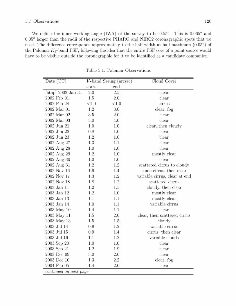
5.1 Observations 120
We define the inner working angle (IWA) of the survey to be 0.55′′. This is 0.065′′ and0.05′′ larger than the radii of the respective PHARO and NIRC2 coronagraphic spots that weused. The difference corresponds approximately to the half-width at half-maximum (0.05′′) ofthe Palomar KS-band PSF, following the idea that the entire PSF core of a point source wouldhave to be visible outside the coronagraphic for it to be identified as a candidate companion.
Table 5.1: Palomar Observations
Date (UT) V -band Seeing (arcsec) Cloud Coverstart end
[htop] 2002 Jan 31 2.0 2.5 clear2002 Feb 01 1.5 2.0 clear2002 Feb 28 <1.0 <1.0 cirrus2002 Mar 01 1.2 3.0 clear, fog2002 Mar 02 3.5 2.0 clear2002 Mar 03 3.0 4.0 clear2002 Jun 21 1.0 1.0 clear, then cloudy2002 Jun 22 0.8 1.0 clear2002 Jun 23 1.2 1.0 clear2002 Aug 27 1.3 1.1 clear2002 Aug 28 1.0 1.0 clear2002 Aug 29 1.2 1.0 mostly clear2002 Aug 30 1.0 1.0 clear2002 Aug 31 1.2 1.2 scattered cirrus to cloudy2002 Nov 16 1.9 1.4 some cirrus, then clear2002 Nov 17 1.3 1.2 variable cirrus, clear at end2002 Nov 18 1.8 1.2 scattered cirrus2003 Jan 11 1.2 1.5 cloudy, then clear2003 Jan 12 1.2 1.0 mostly clear2003 Jan 13 1.1 1.1 mostly clear2003 Jan 14 1.0 1.1 variable cirrus2003 May 10 1.4 1.1 clear2003 May 11 1.5 2.0 clear, then scattered cirrus2003 May 13 1.5 1.5 cloudy2003 Jul 14 0.9 1.2 variable cirrus2003 Jul 15 0.9 1.4 cirrus, then clear2003 Jul 16 1.1 1.2 variable clouds2003 Sep 20 1.0 1.0 clear2003 Sep 21 1.2 1.9 clear2003 Dec 09 3.0 2.0 clear2003 Dec 10 1.3 2.2 clear, fog2004 Feb 05 1.4 2.0 clearcontinued on next page

5.1 Observations 121
Table 5.1–continued from previous pageDate (UT) V -band Seeing (arcsec) Cloud Cover
start end2004 Feb 06 3.0 2.3 variable cirrus2004 Feb 07 0.9 1.5 thin cirrus, then clear2004 Jun 04 1.0 0.8 clear2004 Jun 26 1.2 1.1 mostly clear2004 Jun 27 1.4 1.0 clear2004 Jun 28 1.2 1.1 clear2004 Oct 03 0.9 0.9 clear2004 Oct 04 1.0 1.0 clear2004 Oct 05 1.0 1.0 clear2005 Jan 24 1.6 1.6 clear for 0.5 hrs, then closed
Table 5.2: Keck Observations
Date V -band Seeing Cloud Cover(UT) (arcsec)2003 May 16 0.7 clear, then cirrus2003 May 17 1.0 partly cloudy2003 May 18 1.0 cirrus2003 Nov 09 0.7 some cirrus2003 Nov 10 0.5 cirrus, then clear2004 Jun 05 1.0 clear2004 Jun 06 0.8 clear2004 Oct 07 0.8 some cirrus2004 Oct 08 1.2 cirrus, sometimes thick
Observations of the 101 stars in the deep sample were obtained at Palomar and/or Keck,with a total of 48 of these observed at Keck. The Keck observations were generally conductedto follow-up candidate companions from prior-epoch imaging at Palomar. However, 7 starswere observed coronagraphically only at Keck. The 165 stars in the shallow sample wereobserved only at Palomar. Tables 5.3 and 5.4 list the epochs and mode of imaging observationsfor all stars in the deep and shallow samples. Stars determined to be single during the first(“discovery”) imaging epoch were not followed up. Stars showing candidate companions werere-imaged at later epochs, where multiple follow-up visits were paid to stars with small propermotions to better constrain the likelihood of association between any of the field objects andthe primary.
The Palomar coronagraphic observations nominally amounted to 24 min of on-source inte-gration time at KS band during the discovery epoch. When the brightness of the candidatecompanions allowed it, subsequent imaging at Palomar was shallower. For Keck observationsthe total KS exposure time was 6 min, which resulted in similar or greater depth of imaging,compared to Palomar. In cases when the depth of the Palomar discovery epoch images wasinadequate because of insufficient exposure time or poor weather, a repeated deep image was

5.1 Observations 122
attempted at a later epoch, at either Palomar or Keck. Thus, most of the targets in the deepsample were imaged to the nominal depth of the survey. This was not achieved only for 11deep-sample stars, which were observed only at Palomar for less than 24 min each and/or inpoor weather. Such stars have entries in the ‘Notes’ column of Table 5.3, where we have speci-fied the length of the total exposure (if <24 min) at each epoch of observations, and whetherthe imaging quality was poor.
Additional limitations on the imaging depth of the Palomar observations dependent on thechoice of Lyot stop and attenuating optic are discussed in §5.1.1. Section §5.1.2 discusses thecorresponding details for the Keck observations. The two sections also present calibrations ofthe near-IR transmissivities of relevant attenuating optics: the PHARO ND 1% filter and theNIRC2 coronagraphic spots. Tables 5.1 and 5.2 list the observation epochs at Palomar and Keck,respectively, along with notes on the atmospheric conditions for each night of observations.
In the final part (§5.1.3) of this section, we discuss in greater detail than addressed in§3.3.2.1.1 the benefits and limitations of the CR rotation approach to imaging at Palomar.
Table 5.3: Deep Sample Observations
Star UT Date Observatory Optic Lyot Stop NotesHD 377 2002-08-28 Palomar corona Medium cross
2003-11-09 Keck corona deepest2004-10-07 Keck corona
HD 691 2002-08-31 Palomar corona Medium cross2002-11-18 Palomar corona Medium cross deepest
HD 984 2002-08-29 Palomar corona Medium cross deepest2003-09-20 Palomar corona Medium cross2004-10-04 Palomar corona Medium cross
HD 1405 2004-06-06 Keck corona deepestQT And 2002-08-29 Palomar corona Medium cross
2003-11-10 Keck corona deepest2004-10-07 Keck corona
HD 7661 2002-08-30 Palomar corona Medium cross2002-11-09 Keck corona deepest
HIP 6276 2002-08-30 Palomar corona Medium cross deepest2004-10-08 Keck corona
HD 8907 2002-08-27 Palomar corona Medium cross deepestHD 12039 2002-08-28 Palomar corona Medium cross 13 min, deepestHD 15526 2003-09-20 Palomar corona Medium cross deepest1RXS J025216.9+361658 2002-11-18 Palomar corona Medium cross
2003-11-10 Keck corona deepest2004-02-07 Palomar corona Medium cross
HD 17925 2003-09-21 Palomar corona Medium cross deepest1RXS J025751.8+115759 2002-11-16 Palomar corona Medium cross deepestRX J0258.4+2947 2002-02-28 Palomar corona Big cross deepest1RXS J030759.1+302032 2002-11-18 Palomar corona Medium cross deepestHD 19668 2002-08-27 Palomar corona Medium cross
2003-11-09 Keck corona deepest1E 0307.4+1424 2003-01-12 Palomar corona Medium cross deepestcontinued on next page

5.1 Observations 123
Table 5.3–continued from previous pageStar UT Date Observatory Extra Optic Lyot Stop NotesAP 93 2003-09-20 Palomar Medium cross
2004-10-03 Palomar Medium cross2004-10-08 Keck corona deepest
1RXS J031907.4+393418 2002-08-29 Palomar corona Medium cross2003-11-10 Keck corona deepest2004-10-08 Keck corona
HE 622 2003-09-20 Palomar Medium cross2004-10-08 Keck corona deepest
1E 0324.1–2012 2003-01-12 Palomar corona Medium cross poor2004-02-07 Palomar corona Medium cross2004-10-08 Keck corona deepest
RX J0329.1+0118 2003-09-21 Palomar corona Medium cross deepestHE 1101 2003-09-20 Palomar Medium cross
2004-10-03 Palomar Medium cross2004-10-07 Keck corona deepest
HD 22179 2002-11-16 Palomar corona Medium cross2003-11-09 Keck corona deepest2004-02-07 Palomar corona Medium cross2004-10-08 Keck corona
HD 23208 2004-10-05 Palomar corona Medium cross deepestHII 120 2003-09-20 Palomar Medium cross
2004-10-04 Palomar Medium cross2004-10-08 Keck corona deepest
HII 2147 2003-01-13 Palomar corona Medium cross deepest1RXS J035028.0+163121 2002-11-17 Palomar corona Medium cross deepestRX J0354.4+0535 2003-01-13 Palomar corona Medium cross
2004-02-07 Palomar Medium cross2004-10-07 Keck corona deepest
Pels 191 2002-11-18 Palomar corona Medium cross 10 min, deepestRX J0357.3+1258 2003-01-11 Palomar corona Medium cross
2003-11-09 Keck corona deepest2004-02-07 Palomar corona Medium cross
HD 285751 2002-01-31 Palomar corona Big cross deepestRX J0442.5+0906 2003-01-11 Palomar corona Medium cross deepest
2004-02-07 Palomar Medium crossHD 286179 2002-01-31 Palomar corona Big cross
2004-02-07 Palomar Medium cross2004-10-07 Keck corona deepest
HD 31950 2002-11-16 Palomar corona Medium cross2003-11-09 Keck corona deepest2004-02-07 Palomar corona Medium cross2004-10-08 Keck corona
HD 35850 2002-02-01 Palomar corona Big cross deepestHD 36869 2003-01-14 Palomar corona Medium cross deepest
2004-10-05 Palomar ND1 Medium cross1RXS J053650.0+133756 2002-02-28 Palomar corona Big cross
2003-01-14 Palomar corona Medium cross2003-11-10 Keck corona deepest
HD 245567 2002-11-16 Palomar corona Medium cross2003-11-09 Keck corona2004-02-07 Palomar corona Medium cross2004-10-08 Keck corona deepest
continued on next page
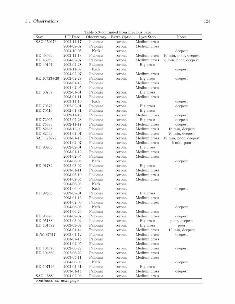
5.1 Observations 124
Table 5.3–continued from previous pageStar UT Date Observatory Extra Optic Lyot Stop NotesSAO 150676 2002-11-17 Palomar corona Medium cross
2004-02-07 Palomar corona Medium cross2004-10-08 Keck corona deepest
HD 38949 2002-11-18 Palomar corona Medium cross 16 min, poor, deepestHD 43989 2004-02-07 Palomar corona Medium cross 8 min, poor, deepestHD 49197 2002-02-28 Palomar corona Big cross
2003-11-09 Keck corona deepest2004-02-07 Palomar corona Medium cross
RE J0723+20 2002-02-28 Palomar corona Big cross deepest2003-01-13 Palomar Medium cross2004-02-05 Palomar Medium cross
HD 60737 2002-01-31 Palomar corona Big cross2003-01-11 Palomar corona Medium cross2003-11-10 Keck corona deepest
HD 70573 2002-02-01 Palomar corona Big cross deepestHD 70516 2002-01-31 Palomar corona Big cross
2002-11-16 Palomar corona Medium cross deepestHD 72905 2002-02-28 Palomar corona Big cross deepestHD 75393 2002-11-17 Palomar corona Medium cross deepestHD 82558 2003-12-09 Palomar corona Medium cross 18 min, deepestHD 82443 2004-02-07 Palomar corona Medium cross 20 min, deepestSAO 178272 2003-01-13 Palomar corona Medium cross 19 min, poor, deepest
2004-02-07 Palomar corona Medium cross 6 min, poorHD 90905 2002-02-01 Palomar corona Big cross
2003-01-12 Palomar corona Medium cross2004-02-05 Palomar corona Medium cross2004-06-05 Keck corona deepest
HD 91782 2002-03-02 Palomar corona Big cross2003-01-11 Palomar corona Medium cross2003-05-10 Palomar corona Medium cross2004-02-05 Palomar corona Medium cross2004-06-05 Keck corona2004-06-06 Keck corona deepest
HD 92855 2002-02-01 Palomar corona Big cross2003-01-13 Palomar corona Medium cross2004-02-06 Palomar corona Medium cross2004-06-06 Keck corona deepest2004-06-26 Palomar corona Medium cross
HD 93528 2004-02-07 Palomar corona Medium cross deepestHD 95188 2002-03-02 Palomar corona Big cross poor, deepestHD 101472 2002-03-02 Palomar corona Big cross poor
2003-01-14 Palomar corona Medium cross 12 min, deepestBPM 87617 2003-01-12 Palomar corona Medium cross deepest
2003-07-16 Palomar Medium cross2004-02-05 Palomar Medium cross
HD 104576 2002-06-22 Palomar corona Medium cross deepestHD 104860 2002-06-23 Palomar corona Medium cross
2003-05-11 Palomar corona Medium cross2004-06-05 Keck corona deepest
HD 107146 2002-01-31 Palomar corona Big cross2003-01-14 Palomar corona Medium cross deepest
SAO 15880 2004-02-06 Palomar corona Medium crosscontinued on next page

5.1 Observations 125
Table 5.3–continued from previous pageStar UT Date Observatory Extra Optic Lyot Stop Notes
2004-06-06 Keck corona deepestSAO 2085 2004-02-07 Palomar corona Medium cross deepestHD 111456 2004-02-06 Palomar corona Medium cross deepestHD 132173 2002-02-28 Palomar corona Big cross
2004-02-07 Palomar corona Medium cross deepestHD 139813 2002-02-01 Palomar corona Big cross
2003-05-17 Keck corona2003-05-18 Keck corona deepest
HD 139498 2003-07-15 Palomar Medium cross2004-06-26 Palomar corona Medium cross deepest
HD 142361 2002-06-21 Palomar corona Medium cross 18 min, deepest2003-07-16 Palomar ND1 Medium cross2004-06-27 Palomar ND1 Medium cross
HD 143006 2002-06-23 Palomar corona Medium cross2003-05-18 Keck corona2004-06-05 Keck corona deepest
(PZ99) J155847.8–175800 2004-06-06 Keck corona deepestScoPMS 21 2002-06-22 Palomar corona Medium cross
2004-06-05 Keck corona deepest(PZ99) J160302.7–180605 2003-05-18 Keck corona
2004-06-06 Keck corona deepestScoPMS 27 2004-06-28 Palomar corona Medium cross deepestScoPMS 52 2002-08-31 Palomar corona Medium cross deepest
2004-06-26 Palomar Medium cross(PZ99) J161318.6–221248 2002-06-21 Palomar corona Medium cross
2003-05-18 Keck corona2004-06-05 Keck corona deepest
(PZ99) J161402.1–230101 2003-07-15 Palomar Medium cross2004-06-05 Keck corona deepest
(PZ99) J161411.0–230536 2002-06-21 Palomar corona Medium cross 6 min2004-06-05 Keck corona deepest
(PZ99) J161459.2–275023 2003-07-15 Palomar Medium cross2004-06-05 Keck corona deepest
(PZ99) J161618.0–233947 2004-06-27 Palomar corona Medium cross deepestHD 146516 2003-05-10 Palomar Medium cross
2004-06-05 Keck corona deepestScoPMS 214 2002-08-30 Palomar corona Medium cross
2004-06-05 Keck corona deepest2004-06-27 Palomar corona Medium cross
HD 151798 2002-06-21 Palomar corona Medium cross 12 min2003-05-16 Keck corona deepest2004-06-26 Palomar corona Medium cross 12 min
HD 165590 2004-06-28 Palomar corona Medium cross deepestHD 166181 2004-06-06 Keck corona deepestHD 170778 2004-06-27 Palomar corona Medium cross deepestHD 171488 2004-06-06 Keck corona deepest
2004-10-08 Keck coronaHD 172649 2002-06-21 Palomar Medium cross
2002-08-31 Palomar corona Medium cross deepest2003-05-13 Palomar Medium cross2003-05-18 Keck corona2004-06-05 Keck corona
continued on next page

5.1 Observations 126
Table 5.3–continued from previous pageStar UT Date Observatory Extra Optic Lyot Stop NotesHD 187748 2004-06-27 Palomar corona Medium cross deepestHD 191089 2003-09-20 Palomar corona Medium cross
2004-06-26 Palomar corona Medium cross deepestHD 199019 2002-08-29 Palomar corona Medium cross deepestHD 200746 2003-09-21 Palomar corona Medium cross 6 min
2004-06-26 Palomar corona Medium cross 4 min, deepestHD 203030 2002-08-28 Palomar corona Medium cross deepest
2003-07-16 Palomar corona Medium cross2004-06-26 Palomar corona Medium cross
HD 209393 2002-11-17 Palomar corona Medium cross deepest2003-09-20 Palomar corona Medium cross2004-10-07 Keck corona
HD 209779 2002-11-16 Palomar corona Medium cross deepestV383 Lac 2002-08-27 Palomar corona Medium cross
2003-07-16 Palomar corona Medium cross2003-11-09 Keck corona deepest
HD 217343 2003-09-21 Palomar corona Medium cross deepestHD 218738 2003-12-10 Palomar corona Medium cross
2004-10-04 Palomar corona Medium cross deepestHD 218739 2003-12-10 Palomar corona Medium cross
2004-10-04 Palomar corona Medium cross deepestHD 219498 2002-08-30 Palomar corona Medium cross deepest
2003-09-20 Palomar corona Medium cross2004-10-05 Palomar corona Medium cross
Table 5.4: Shallow Sample Observations
Star UT Date Observatory Optic Lyot Stop NotesHD 224873 2002-08-31 Palomar ND1 Medium cross
2003-09-21 Palomar ND1 Medium crossHD 9472 2002-11-18 Palomar ND1 Medium cross
2003-09-20 Palomar ND1 Medium cross2004-10-05 Palomar ND1 Medium cross
RE J0137+18A 2002-01-31 Palomar Big cross2003-09-20 Palomar ND1 Medium cross
HD 13507 2002-08-28 Palomar corona Medium cross 18 minHD 13531 2002-08-28 Palomar ND1 Medium cross
2003-09-21 Palomar ND1 Medium cross2004-10-05 Palomar ND1 Medium cross
1RXS J025223.5+372914 2003-09-21 Palomar Medium cross2004-10-05 Palomar Medium cross
2RE J0255+474 2002-02-28 Palomar Big cross2004-10-05 Palomar Medium cross
HD 18940 2002-08-29 Palomar ND1 Medium crossHD 19632 2002-08-30 Palomar Medium crossvB 1 2002-08-29 Palomar ND1 Medium crossHE 350 2003-09-20 Palomar Medium crosscontinued on next page
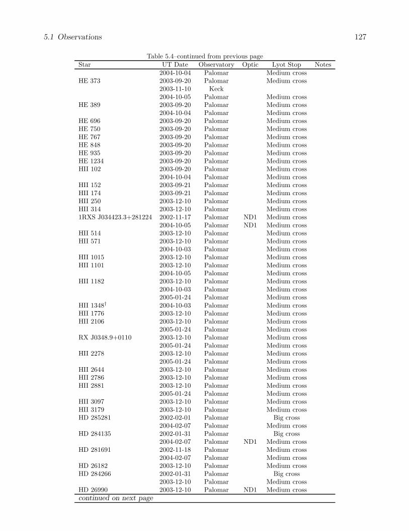
5.1 Observations 127
Table 5.4–continued from previous pageStar UT Date Observatory Optic Lyot Stop Notes
2004-10-04 Palomar Medium crossHE 373 2003-09-20 Palomar Medium cross
2003-11-10 Keck2004-10-05 Palomar Medium cross
HE 389 2003-09-20 Palomar Medium cross2004-10-04 Palomar Medium cross
HE 696 2003-09-20 Palomar Medium crossHE 750 2003-09-20 Palomar Medium crossHE 767 2003-09-20 Palomar Medium crossHE 848 2003-09-20 Palomar Medium crossHE 935 2003-09-20 Palomar Medium crossHE 1234 2003-09-20 Palomar Medium crossHII 102 2003-09-20 Palomar Medium cross
2004-10-04 Palomar Medium crossHII 152 2003-09-21 Palomar Medium crossHII 174 2003-09-21 Palomar Medium crossHII 250 2003-12-10 Palomar Medium crossHII 314 2003-12-10 Palomar Medium cross1RXS J034423.3+281224 2002-11-17 Palomar ND1 Medium cross
2004-10-05 Palomar ND1 Medium crossHII 514 2003-12-10 Palomar Medium crossHII 571 2003-12-10 Palomar Medium cross
2004-10-03 Palomar Medium crossHII 1015 2003-12-10 Palomar Medium crossHII 1101 2003-12-10 Palomar Medium cross
2004-10-05 Palomar Medium crossHII 1182 2003-12-10 Palomar Medium cross
2004-10-03 Palomar Medium cross2005-01-24 Palomar Medium cross
HII 1348† 2004-10-03 Palomar Medium crossHII 1776 2003-12-10 Palomar Medium crossHII 2106 2003-12-10 Palomar Medium cross
2005-01-24 Palomar Medium crossRX J0348.9+0110 2003-12-10 Palomar Medium cross
2005-01-24 Palomar Medium crossHII 2278 2003-12-10 Palomar Medium cross
2005-01-24 Palomar Medium crossHII 2644 2003-12-10 Palomar Medium crossHII 2786 2003-12-10 Palomar Medium crossHII 2881 2003-12-10 Palomar Medium cross
2005-01-24 Palomar Medium crossHII 3097 2003-12-10 Palomar Medium crossHII 3179 2003-12-10 Palomar Medium crossHD 285281 2002-02-01 Palomar Big cross
2004-02-07 Palomar Medium crossHD 284135 2002-01-31 Palomar Big cross
2004-02-07 Palomar ND1 Medium crossHD 281691 2002-11-18 Palomar Medium cross
2004-02-07 Palomar Medium crossHD 26182 2003-12-10 Palomar Medium crossHD 284266 2002-01-31 Palomar Big cross
2003-12-10 Palomar Medium crossHD 26990 2003-12-10 Palomar ND1 Medium crosscontinued on next page

5.1 Observations 128
Table 5.4–continued from previous pageStar UT Date Observatory Optic Lyot Stop Notes
2005-01-24 Palomar ND1 Medium crossvB 39 2003-01-12 Palomar Medium crossvB 49 2003-01-12 Palomar Medium crossvB 52 2003-01-12 Palomar Medium cross
2004-10-05 Palomar ND1 Medium crossvB 176 2003-12-10 Palomar Medium cross
2004-10-03 Palomar ND1 Medium crossvB 63 2003-01-12 Palomar Medium crossvB 66 2002-11-17 Palomar corona Medium crossvB 73 2003-01-12 Palomar Medium crossvB 180 2003-12-10 Palomar Medium crossvB 88 2003-12-10 Palomar Medium cross1RXS J043243.2–152003 2003-01-12 Palomar Medium crossvB 91 2003-12-10 Palomar Medium cross
2004-10-03 Palomar ND1 Medium crossvB 96 2003-12-10 Palomar Medium crossRX J0434.3+0226 2003-01-12 Palomar Medium cross poorvB 106 2003-12-10 Palomar Medium cross
2004-10-05 Palomar corona Medium crossHD 282346 2002-11-18 Palomar Medium cross
2004-10-04 Palomar ND1 Medium crossvB 142 2002-11-17 Palomar corona Medium cross
2003-11-10 Keck corona2004-02-07 Palomar corona Medium cross
HD 286264 2003-12-10 Palomar Medium cross1RXS J051111.1+281353 2002-02-28 Palomar Big cross
2003-01-14 Palomar Medium cross2003-12-10 Palomar Medium cross
HD 37006 2003-01-11 Palomar Medium cross2003-12-10 Palomar Medium cross
HD 61994 2002-11-18 Palomar ND1 Medium crossHD 66751 2002-11-18 Palomar ND1 Medium crossHD 69076 2002-11-18 Palomar ND1 Medium cross
2003-05-11 Palomar ND1 Medium cross2004-02-06 Palomar Medium cross
HD 71974 2002-03-03 Palomar Big crossHD 72687 2003-12-09 Palomar ND1 Medium crossHD 72760 2002-11-16 Palomar ND1 Medium crossHD 73668 2002-05-11 Palomar corona Medium cross
2004-02-06 Palomar Medium crossHD 77407 2002-01-31 Palomar Big cross
2003-01-13 Palomar ND1 Medium cross2003-05-10 Palomar ND1 Medium cross
HD 78899 2003-12-09 Palomar ND1 Medium crossHD 88638 2002-01-31 Palomar corona Big cross 17 minHD 91962 2002-03-02 Palomar Big cross
2003-05-10 Palomar ND1 Medium cross2004-02-05 Palomar ND1 Medium cross
HD 98553 2003-01-11 Palomar Medium crossHD 99565 2003-01-11 Palomar ND1 Medium cross
2003-05-11 Palomar ND1 Medium cross2004-02-05 Palomar ND1 Medium cross
HD 100167 2002-03-03 Palomar corona Big cross poorcontinued on next page

5.1 Observations 129
Table 5.4–continued from previous pageStar UT Date Observatory Optic Lyot Stop NotesHD 101959 2002-02-28 Palomar Big crossHD 102071 2002-02-28 Palomar Big crossHD 108799 2003-05-10 Palomar ND1 Medium cross
2003-07-16 Palomar ND1 Medium cross2004-02-05 Palomar ND1 Medium cross2004-06-26 Palomar ND1 Medium cross
HD 108944 2002-03-03 Palomar Big cross2002-06-21 Palomar Medium cross2003-01-13 Palomar ND1 Medium cross2003-05-11 Palomar ND1 Medium cross2004-02-05 Palomar ND1 Medium cross2004-06-27 Palomar ND1 Medium cross
HD 112196 2002-02-01 Palomar Big cross2003-01-13 Palomar ND1 Medium cross2003-05-11 Palomar ND1 Medium cross2004-02-05 Palomar ND1 Medium cross2004-06-26 Palomar ND1 Medium cross
HD 115043 2003-12-09 Palomar ND1 Medium cross2004-06-27 Palomar ND1 Medium cross
HD 129333 2003-01-11 Palomar ND1 Medium cross2003-01-12 Palomar ND1 Medium cross2003-05-13 Palomar Medium cross2004-02-05 Palomar ND1 Medium cross
HD 133295 2002-02-28 Palomar Big crossHD 134319 2002-03-02 Palomar Big cross poor
2003-01-14 Palomar ND1 Medium cross2004-06-27 Palomar ND1 Medium cross
HD 135363 2002-02-01 Palomar Big cross2003-01-14 Palomar ND1 Medium cross2004-06-27 Palomar ND1 Medium cross
RX J1541.1–2656 2003-07-15 Palomar Medium cross2004-06-27 Palomar Medium cross
RX J1600.6–2159 2003-07-15 Palomar Medium cross(PZ99) J160814.7–190833 2002-08-31 Palomar Medium cross(PZ99) J161329.3–231106 2003-05-10 Palomar Medium cross
2004-06-26 Palomar Medium crossHD 150554 2003-05-10 Palomar ND1 Medium cross
2003-07-16 Palomar ND1 Medium crossHD 152555 2002-08-31 Palomar ND1 Medium cross
2003-07-16 Palomar ND1 Medium cross2004-06-26 Palomar ND1 Medium cross
HD 155902 2003-09-21 Palomar ND1 Medium crossHD 157664 2003-05-10 Palomar corona Medium cross
2004-10-04 Palomar ND1 Medium crossHD 166435 2002-06-23 Palomar corona Medium cross
2002-08-30 Palomar corona Medium cross2003-05-16 Keck corona2004-06-26 Palomar corona Medium cross
HD 167389 2003-05-13 Palomar ND1HD 175742 2004-06-28 Palomar corona Medium crossHD 193216 2003-07-16 Palomar corona Medium cross 12 min, poor
2004-06-27 Palomar corona Medium cross 12 minHD 199143 2002-06-23 Palomar ND1 Medium crosscontinued on next page
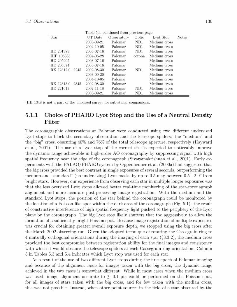
5.1 Observations 130
Table 5.4–continued from previous pageStar UT Date Observatory Optic Lyot Stop Notes
2003-09-21 Palomar ND1 Medium cross2004-10-05 Palomar ND1 Medium cross
HD 201989 2003-07-16 Palomar ND1 Medium crossHIP 106335 2004-06-28 Palomar corona Medium crossHD 205905 2003-07-16 Palomar Medium crossHD 206374 2003-07-16 Palomar Medium crossRX J2312.0+2245 2002-08-30 Palomar ND1 Medium cross
2003-09-20 Palomar Medium cross2004-10-05 Palomar Medium cross
RX J2313.0+2345 2002-08-30 Palomar Medium crossHD 221613 2002-11-18 Palomar ND1 Medium cross
2003-09-21 Palomar ND1 Medium cross
†HII 1348 is not a part of the unbiased survey for sub-stellar companions.
5.1.1 Choice of PHARO Lyot Stop and the Use of a Neutral DensityFilter
The coronagraphic observations at Palomar were conducted using two different undersizedLyot stops to block the secondary obscuration and the telescope spiders: the “medium” andthe “big” cross, obscuring 40% and 76% of the total telescope aperture, respectively (Haywardet al., 2001). The use of a Lyot stop of the correct size is expected to noticeably improvethe dynamic range achievable in high-order AO coronagraphy by suppressing signal with highspatial frequency near the edge of the coronagraph (Sivaramakrishnan et al., 2001). Early ex-periments with the PALAO/PHARO system by Oppenheimer et al. (2000a) had suggested thatthe big cross provided the best contrast in single exposures of several seconds, outperforming themedium and “standard” (no undersizing) Lyot masks by up to 0.5 mag between 0.5′′–2.0′′ frombright stars. However, our experience from observing each star in multiple longer exposures wasthat the less oversized Lyot stops allowed better real-time monitoring of the star-coronagraphalignment and more accurate post-processing image registration. With the medium and thestandard Lyot stops, the position of the star behind the coronagraph could be monitored bythe location of a Poisson-like spot within the dark area of the coronagraph (Fig. 5.1): the resultof constructive interference of high spatial frequency light pushed to the periphery of the Lyotplane by the coronagraph. The big Lyot stop likely shutters that too aggressively to allow theformation of a sufficiently bright Poisson spot. Because image registration of multiple exposureswas crucial for obtaining greater overall exposure depth, we stopped using the big cross afterthe March 2002 observing run. Given the adopted technique of rotating the Cassegrain ring to4 mutually orthogonal orientations during the imaging of each star (§3.3.2), the medium crossprovided the best compromise between registration ability for the final images and consistencywith which it would obscure the telescope spiders at each Cassegrain ring orientation. Column5 in Tables 5.3 and 5.4 indicates which Lyot stop was used for each star.
As a result of the use of two different Lyot stops during the first epoch of Palomar imagingand because of the alignment issue for images taken with the big cross, the dynamic rangeachieved in the two cases is somewhat different. While in most cases when the medium crosswas used, image alignment accurate to . 0.1 pix could be performed on the Poisson spot,for all images of stars taken with the big cross, and for few taken with the median cross,this was not possible. Instead, when other point sources in the field of a star obscured by the

5.1 Observations 131
(b)
waffle speckles
Poisson Spot
(a)
waffle
speckles
1"
Figure 5.1: Close-up sample images with the big (a) and medium (b) Lyot stops, using the0.97′′ coronagraph. Characteristic features of the PALAO PSF are indicated with arrows. Themedium Lyot stop allows the formation of a Poisson spot at the location of the star, enablingconsistent image registration.
Table 5.5: Magnitude Extinction due to PHARO and NIRC2 Optics
Transmissive Optic ∆J ∆H ∆KS
PHARO ND 1% filter 4.753 ± 0.039 4.424 ± 0.033 4.197 ± 0.024NIRC2 1′′ coronagraph 8.36 ± 0.28 7.78 ± 0.15 7.10 ± 0.17NIRC2 2′′ coronagraph 9.26 ± 0.09 7.79 ± 0.22 7.07 ± 0.22
coronagraph were visible in the individual short exposures, these sources were used as referencesfor registration. However, for 17 stars (17% of the sample) showing no candidate companions,we had to rely on cross-correlation techniques, which had poorer positional accuracy (0.5 pix;§4.6). As a result, these 17 images are, on average, 0.23 mag shallower. This factor has beentaken into account in the calculation of the ensemble survey detection limits (§5.2).
The non-coronagraphic observations at Palomar were also performed with two differentsettings: with and without a 1% neutral density (ND) filter in the beam path. The NDfilter was used for imaging stars brighter than KS = 7 − 8 mag (depending on atmospherictransparency) to prevent detector saturation. This is noted accordingly with an “ND1” entryin column 4 of Tables 5.3 and 5.4. Fainter stars were observed without the filter. The use ofthe ND filter does not have a measurable effect on the overall contrast. However, it furtherlimits the depth of non-coronagraphic exposures. We calibrated the near-IR extinction of theND 1% filter from relative photometric measurements of three program stars with and withoutthe ND filter. The calibration results are tabulated in Table 5.5. The Lyot stop setting for thenon-coronagraphic exposures was left as in the coronagraphic observations.
5.1.2 Choice of NIRC2 Coronagraphs and Pupil Mask
Images with NIRC2 were obtained only in coronagraphic mode, using predominantly the 1′′-diameter spot, though the 2′′-diameter spot was used during the May 16–18, 2003, observingrun. Unlike the PHARO coronagraphic spots, the NIRC2 spots are transmissive, offering the
5.1 Observations 132
possibility to obtain accurate relative positioning and approximate photometry with respectto the primary. A measurement of the throughput of the 2′′ spot was already presented in§3.3.3.1. Subsequent observations showed that such measurements are dependent on the qualityof the AO correction, possibly because of the amount of spill-over light behind the edge of thecoronagraph. Thus, approximate relative photometry with the NIRC2 coronagraph is likelyfeasible only with good AO correction (usually at H and K band), when spill-over behind thecoronagraph is minimized. Table 5.5 lists the measured near-IR extinction in magnitudes forthe 1′′ and 2′′ NIRC2 coronagraphs. The large apparent difference in the J-band transmissivityof the two coronagraphic spots is a probable effect of spillover, aggravated by poorer AOperformance at J .
Similarly to PHARO, NIRC2 offers a selection of undersized hexagonal and circular pupilmasks to occult the mirror edges, though not the telescope spiders. Among those we chosethe “inscribed circle” mask, which corresponds to the largest circular aperture inscribed in thetelescope mirror. This mask has a 90.7% clear area and provides round, rather than hexagonal,PSFs—a factor that was deemed important for aperture photometry and centering.
5.1.3 Rotating the Cassegrain Ring at Palomar: The Cons Outweighthe Pros
Identifying faint objects in the haloes of bright stars is one of the principal directions of modernastronomy. The main challenge is to remove the contribution of the PSF as close to the star aspossible, and bring down the residual noise as close to the photon noise limit as possible. Variousexperimental techniques of PSF subtraction with advanced AO systems are currently beingtested, such as simultaneous differential imaging (Racine et al., 1999; Close, 2004; Marois et al.,2005) and differential polarimetry (Kuhn et al., 2001; Apai et al., 2004). With conventionalAO, the best approaches involve either image rotation followed by “roll-angle” subtraction, orthe observation of a suitable PSF standard star. Both in principle allow the subtraction of thePSF to within a factor of ∼3–5 of the photon noise limit, beyond which imperfect eliminationof speckles dominates the noise. The former is the method of choice for altitude-azimuth (alt-az) telescopes (e.g., Keck), as the sky can by allowed to rotate in between exposures whilekeeping the PSF fixed with respect to the detector (i.e., when imaging in “vertical angle”mode). The difference of two images taken at different sky position angles provides nearly asgood a subtraction of the PSF as is possible with conventional AO. The PSF standard starapproach is better suited to telescopes on equatorial mounts, where, if no additional imageplane rotation capability exists, the position angle of the sky is constant. Observing separatePSF stars is often undesirable, however, as it adds 100% overhead.
We initially saw the ability to rotate the Hale telescope CR ring as an opportunity to mimicalt-az behavior at Palomar and thus maintain high observing efficiency, without needing toobserve PSF stars. Because the CR carries both PALAO and PHARO (containing most ofthe intermediate optics), most of the PSF artifacts induced in the optical train were expectedto retain a constant orientation on the detector, while the sky position angle changes. Theonly difference with a true alt-az telescope would be the fact that the telescope primary andsecondary mirrors, and the secondary support spiders, will rotate with respect to the detector.We believed that the use of an aggressive Lyot stop, such as the medium or big cross, tocover the mirror edges and the spiders, would adequately limit this undesirable effect. Byrotating through 90, we planned to ensure constant alignment of the support spiders with

5.1 Observations 133
the Lyot stop mask. Discussions with Tom Hayward and Stephen Eikenberry, both extensiveusers of the PALAO system at the time, suggested that this may be a viable, albeit previouslyunexplored approach.
The procedure was adopted without extensive testing, and because of the four-corneredsymmetry of the characteristic Shack-Hartmann “waffle” pattern of the PALAO PSF (Fig. 5.1),it appeared that the approach could provide good cancelation at least of the corner wafflespeckles. However, we subsequently discovered that this method does not offer noticeableimprovement over a technique based on a simple rotation (or mirror flipping) of the imagearound the primary, followed by a subtraction of the rotated image. As it turned out, thePSF speckles rotated with the detector, indicating that most of the wavefront aberration wasincurred by the primary and secondary telescope mirrors. The 180-rotation and subtractiontechnique quickly became the method of choice for PSF subtraction for all of the coronagraphicdata. Nevertheless, the CR rotation strategy during observations was maintained, partially forsurvey self-consistency, and partially to mitigate the effect of a large-scale (∼15′′) low surfacebrightness ghost reflection of the telescope pupil, visible in most of the deep coronagraphicexposures. The ghost image did not follow the rotations of the array and could thus be effectivelyremoved by median-combining data from different CR orientations.
The most negative effect of the CR rotations, which went unnoticed for a large fraction ofthe survey duration, had to do with the non-uniformity of the PHARO pixel scale (§4). Theuse of CR rotations limited the imaging depth because when objects were rotated to differentparts of the array images of identical parts of the sky suffered different amounts of focal planedistortion. Thus, images taken at CR angles differing by 90 were not related by a simple90 rotation, but rather by a rotation by 90 + ε and by a position-dependent magnification(§4.4.3). The result was a noticeable smearing of the PSF in the final, un-rotated, median-combined images beyond 4′′–7′′ from the central star. This smearing was initially erroneouslyattributed to anisoplanatism. However, in later images taken under excellent atmosphericconditions, when high (>50%) Strehl ratio PSFs of point sources were obtained out to the edgeof the array (indicating that the isoplanatic angle was much larger than the PHARO field), starsin the array corners appeared as distinct binaries in the final un-rotated image.1 Therefore, inpractice, CR rotations limited the imaging depth at large (& 10′′) separations by a factor of ≈2(0.75 mag). At smaller angular separations the decrease in image depth was marginal and wasclose to 0 mag inwards of ≈4′′, where the differential field distortion between CR orientationswas <2 pix—less than half of the PSF FWHM.
In addition to the negative effect on image depth, because of the sparse detector coveragein the calibration of the pixel scale dependence on the CR angle, the use of CR rotations alsolimits the astrometric precision to a factor of &1.6 from what is optimally attainable whenobserving only at a single CR angle (§4.4.4).
Finally, CR rotations incur some amount of overhead, related to re-acquiring AO lock ateach new CR angle. This was about 3 min per rotation, or 38% of the total on-source exposuretime, for 3 rotations in between 4 distinct CR orientations.
To summarize, the use of CR rotations for deep AO imaging over the entire field of thePHARO detector offers fewer benefits than set-backs. While it does allow the elimination oflarge-scale ghost reflections from the telescope pupil, it overall decreases exposure depth at >5′′
1Although 4 distinct images of the same star should be expected, given that images were taken at 4 sepa-rate CR orientations, diametrically opposite CR orientations seemed to produce similar overall distortions (cf.Fig. 4.7), resulting in pair-wise combination of the 4 expected images.

5.2 Object Detection—Limits 134
separations, has a negative effect on astrometric precision, and adds overhead when compared tosimple staring-mode (i.e., without the use of a standard star) observations. The recommendedapproach, as a result of our experience with PALAO, is to chose pairs of science targets thatare closely separated (.10) on the sky and that are mutually suitable (i.e., have similarbrightness and color) to serve as PSF standards for each other. The technique is appropriatefor coronagraphic surveys of young open clusters, where the density of stars is higher thanin the field. Upon our recommendation, the approach was successfully implemented for thepurpose of the Space Interferometry Mission Planets around Young Stars (PLAYS) key project(P.I. C. Beichman). The PSF-subtracted images showed an improvement in contrast by 0.5–1.0 mag over 0.5′′–3′′ from the host star, compared to the simple rotation and subtractionmethod. Unfortunately, this approach may not be adequate for surveys of widely-separatedsample targets, such as the present one.
5.2 Object Detection—Limits
5.2.1 Automatic Source Detection Is Presently Not Well-suited toHigh-Contrast AO Imaging
Object detection is a straightforward matter to automate in images, in which the PSF is radiallysymmetric, approximately constant in time, and has a well-characterized dependence on imagelocation. This is the case with the majority of ground-based seeing-limited and space-basedobservations. Various approaches are available, such as matched-filtering, localized signal-to-noise calculation, and image deconvolution, to name a few of the most popular ones. Thesehave been implemented in a wide variety of programs, such as DAOPHOT (Stetson, 1987),SExtractor (Bertin & Arnouts, 1996), WAVDETECT (Freeman et al., 2002), findobs inthe ECLIPSE package (Devillard, 2001), StarFinder (Diolaiti et al., 2000), idac (Jefferies& Christou, 1993), etc. These programs are best suited, and often essential, for the detection ofpoint sources in crowded fields. These often contain objects of similar brightness and have a well-characterized spatial PSF behavior. The automated programs are less adequate for fields thatare scarce in sources and where high-contrast is required. In addition, they are not applicableto coronagraphic imaging, where the main (and frequently only) point source is occulted. Theabove limitations describe well the sparsely populated, high-contrast, coronagraphic images inthe present survey.
High-contrast AO imaging presents great difficulties for automated source finding becauseof the large number of speckles in the vicinity of the star (Fig. 5.1). The speckles are individualimages of the star, that form from uncorrected and/or induced (by the telescope optics) aberra-tions in the wavefront and appear indistinguishable from point sources to automated detectionroutines. A vivid example of this is the close-up of the Palomar image of the ∆KS = 8.2 magHD 49197A/B system (Fig. 3.5b), where the companion is drowned in speckle noise. Theexistence of the companion, hinted by a dark ring around one of the speckles with a radius cor-responding to that of the first Airy null radius, was appreciated only after it was discovered in alater-epoch higher-contrast Keck AO image. As a result, even though some of the source detec-tion algorithms listed above have been developed (StarFinder), or adapted (DAOPHOT,idac), for AO image restoration, they did not produce satisfactory results on our images. Ourexperiments with DAOPHOT, WAVDETECT, and StarFinder produced large numbers

5.2 Object Detection—Limits 135
of spurious detections, the vast majority of which could be identified with speckles around thecoronagraph. If the signal-to-noise threshold in the source-finding algorithms was adjusted toa correspondingly higher level, the algorithms would miss the bona fide point sources in thefield. The character of the result did not change whether we used various methods of PSFsubtraction or not. Similar experiences and conclusions are drawn in Carson et al. (2005),who also used the PALAO/PHARO system for their sub-stellar companion search. Therefore,after some experimentation, despite an understanding that automated source detection has thepotential to offer greater repeatability and conceptual clarity, we abandoned the approach.
The remaining option is visual identification. It has been our experience during this sur-vey that, barring subjective factors, visual inspection of images for candidate companions al-ways produces superior results, compared to automated detection. A glance through the high-contrast AO literature re-affirms this. The vast majority of researchers, including the authors ofthe first successful imaging survey for sub-stellar companions (Oppenheimer et al., 2001), have(sometimes grudgingly) ultimately resorted to by-eye identification of candidate companions(Tokovinin et al., 1999; Brandner et al., 2000; Luhman & Jayawardhana, 2002; McCarthy &Zuckerman, 2004; Masciadri et al., 2005; Luhman et al., 2005). Few examples to the contraryexist, in addition to the experiments of Carson et al. (2005). One exception is the study ofLowrance et al. (2005), who apply a rigorous custom-made automated detection scheme totheir NICMOS data. However, the Lowrance et al. survey benefits from the well-behavedPSF of space-borne HST imaging. In a separate instance, Shatsky & Tokovinin (2002) useDAOPHOT II (Stetson, 1992) for their non-coronagraphic AO data. DAOPHOT II allowsadditional cleaning around the PSF and is thus potentially more appropriate for AO data,where the PSF consists of a narrow core and a broad halo. However, Shatsky & Tokovinin donot discuss an application of the approach to their set of coronagraphic data. Finally, Schroederet al. (2000) concede that, after spending several man months in investigating different auto-mated source detection approaches, simple by-eye inspection is most reliable. Therefore, havingfound no better alternative, we adopted visual inspection as the method of choice for identifyingcandidate companions.
5.2.2 Visual Source Detection and Limits
We carefully inspected all of the final coronagraphic images for candidate companions andmeasured their positions and fluxes with the PHOT task in IRAF. The visual inspection wasrepeated multiple times during image reduction, photometry, and astrometry; hence subjectivefactors were brought down to a minimum. We examined the images both prior to, and afterPSF subtraction. At small angular separations PSF subtraction facilitates the detection of faintobjects embedded in the bright halo of the star, while at larger separations (in the background-limited regime) it induces noise and limits their visibility. When a candidate point source wasdetected, the individual 1 min images and the 6 min median-combined images taken at thesame CR angle were inspected to check for the object at the corresponding locations. In mostcases, this was sufficient to distinguish artifacts from bona fide point sources. Still, because ofthe greater depth of the final image (despite some PSF smearing at >4′′ separations), very faintobjects were sometimes not visible in <24 min sub-sets of images. Such candidate companions,less than a dozen overall near the detection limit, were treated as real objects and followed upwith further imaging. Only 3 such objects turned out to be real, as evidenced by deeper Keckimages, though the existence of several still remains undecided.
5.2 Object Detection—Limits 136
We attempted various methods of PSF removal on the final images, including: (1) sub-tracting a median-combined PSF of the star formed from the individual images taken at all4 CR angles, (2) 180 rotation centered on the star and subtraction of the image from itself(§5.1.3), (3) high-pass filtering, in which a Gaussian-smoothed (Gaussian FWHM = 1−3× PSFFWHM) version of the image was subtracted from the original, and (4) simple subtraction ofan azimuthally medianed radial profile. We found that (1–3) gave comparable results, while(4) did not perform as well as the rest because of the four-cornered shape of the PSF. Eventhough (3) is arguably the most widely used method for PSF subtraction when separate PSFobservations are not available, we found that, because of the central symmetry of the bright-est AO speckles (Boccaletti et al., 2002; Bloemhof, 2003), method (2) worked similarly well.Method (2) also did not alter the photon statistics of the PSF-subtracted image in the spatiallycorrelated manner incurred by Gaussian smoothing. We therefore relied on method (2) for themost.
We quantified the ability to detect faint objects as a function of angular separation fromthe star, by randomly introducing artificial point sources of constant (modulo random Poissonnoise) brightness, in a manner analogous to the one described in §3.2.5.1. We performedthe experiment on the reduced coronagraphic and non-coronagraphic survey images of thestar HD 172649, for which the data were taken under good observing conditions with Strehlratios of ≈50%. We introduced 1000–5000 artificial point sources of constant brightness atrandom locations over the entire area of the images and counted the fraction of them thatwere retrievable in 0.25′′–1.0′′-wide concentric annuli centered on the star. We repeated theexperiment for a range of artificial star magnitudes, at steps of 0.5 mag. The PSF for theartificial stars in the unocculted image was obtained from a fit to the primary, whereas in thecoronagraphic image it was obtained from a fit to the brightest field object (∆KS = 6.4 mag).
Figure 5.2 presents the results from the artificial star experiments, where the contrast limitsfrom coronagraphic observations at Palomar and Keck are shown with solid and long-dashedlines, respectively, and the non-coronagraphic limits for Palomar are shown with a short-dashedline. The slow upturn in the Palomar limits (decrease in contrast) at >5′′ separations is due toan additive parameter to model the decreasing exposure depth toward the edge of the PHAROfield, because of image mis-registration among the different CR angles (§5.1.3). The parameteris set to vary linearly between 0 mag and 0.75 mag in the 4–12.5′′ separation range. As is evidentfrom Figure 5.2, under good observing conditions, the 6 min long Keck AO coronagraphic imagesoffered 0.5–1.5 mag higher contrast and depth than the 24 min PALAO images, with the highestdifference being in the 1.0′′–1.5′′ separation range, where the presence of waffle-mode distortionin the PSF limits the contrast at PALAO.
5.2.3 R.M.S. Noise Detection Limits
Often instead of performing artificial star experiments, a seemingly more analytically appealingand straightforward approach is taken, in which the contrast limits are determined in a purelystatistical manner from the r.m.s. deviation σ of the pixel counts in the PSF halo in concentricannuli centered on the star. Five to ten σ is generally regarded as a sufficiently conservativelevel in approximating realistic detection limits.
We implement this approach by constructing an azimuthally-symmetric radial profile of thePSF, equal at each radius to the r.m.s. scatter of the pixel values in 4 pixel wide (0.1′′) annuli.Instead of treating the pixels independently, we normalize their r.m.s. scatter to an aperture
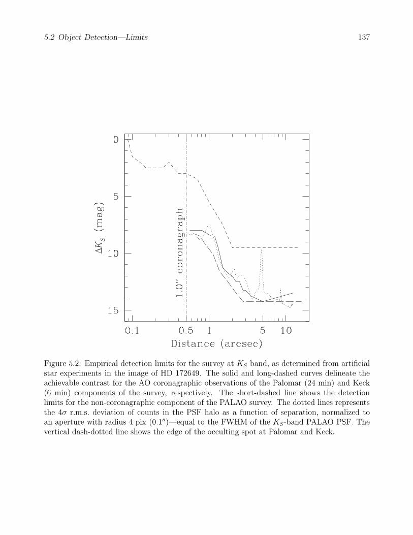
5.2 Object Detection—Limits 137
Figure 5.2: Empirical detection limits for the survey at KS band, as determined from artificialstar experiments in the image of HD 172649. The solid and long-dashed curves delineate theachievable contrast for the AO coronagraphic observations of the Palomar (24 min) and Keck(6 min) components of the survey, respectively. The short-dashed line shows the detectionlimits for the non-coronagraphic component of the PALAO survey. The dotted lines representsthe 4σ r.m.s. deviation of counts in the PSF halo as a function of separation, normalized toan aperture with radius 4 pix (0.1′′)—equal to the FWHM of the KS-band PALAO PSF. Thevertical dash-dotted line shows the edge of the occulting spot at Palomar and Keck.

5.2 Object Detection—Limits 138
of radius equal to the FWHM of the PSF, to match the approximate spatial correlation scalein the image. This procedure imposes a more stringent requirement on the significance of thedetection of a candidate point source by precluding single pixel peaks from dominating annulusstatistics. We show the thus-obtained 4σ r.m.s. noise profile of the halo by the dotted line inFigure 5.2. The bumps and spikes in the dotted line correspond to bright features in the imageof HD 172649, e.g., to the corners of the waffle pattern at 1.0′′ and to projected companions tothe star at 2.1′′, 4.8′′, and 8.6′′. The 4σ line closely follows the visually determined detectionlimits, potentially indicating that the multitude of additive Gaussian and non-Gaussian sourcesof noise in the speckle-limited regime (Racine et al., 1999) may eventually behave in a nearlyGaussian manner because of the central limit theorem. The strongest systematic deviation ofthe 3σ r.m.s. profile from the visually-determined contrast limits is at angular separations >7′′,in the region where the visual limits have been adjusted for CR angle image mis-registration.
The agreement between the detection limits from visual inspection and from r.m.s. statisticsis dependent on a number of factors, such as the radius of the normalization aperture (here equalto 1 FWHM of the PSF), the treatment of point source photon statistics (ignored in this case),and the appropriate functional treatment of non-Gaussian sources of error (speckles, shape ofthe PSF core and halo; also ignored here). Therefore, the 4σ dotted line in Figure 5.2 does notcarry the statistical significance of a confidence level at which 99.997% of random fluctuationsare rejected. However, because of its close representation of the visually-determined detectionlimits, we will use it to build ensemble detection limits on a per-star basis, as in the discussionfollowing section.
5.2.4 Ensemble Detection Limits for the Deep Sample
The empirical detection limits in Figure 5.2 were obtained for observations that benefitedfrom good AO correction (Strehl ratio of ≈50%) on a bright star (V = 7.5) and medianatmospheric conditions for the survey (1.2′′ seeing, scattered cirrus). While high-quality AOperformance on bright stars at Palomar and Keck is now achieved consistently under averageto good atmospheric conditions, fainter stars and worse weather incur a toll on the qualityof the AO correction, expressed in poorer contrast and shallower imaging depth. Indeed, acomparison with the detection limits of the Carson et al. (2005, Fig. 4) PALAO companionsurvey shows that the by-eye contrast limits from Figure 5.2 are similar to their “best 10%”contrast limits (modulo the level of the sky background limit at large separations). The by-eyelimits are ≈2.5 mag deeper than the median sensitivity reported in Carson et al. (2005), and are≈4.5 mag deeper than the authors’ “worst 10%” sensitivity limits. PALAO performance hasundoubtedly improved as a result of several upgrades since 2000–2002, when the Carson et al.(2005) data were taken. In addition, the lowest quality data in our campaign were either re-taken or excluded from the survey. Hence, we do not expect such a dramatic range of sensitivityfor the different images in our survey. Nevertheless, the Carson et al. (2005) result exemplifiesthe need to monitor the achieved contrast on a per-star basis. For the purpose of estimatingthe completeness of the survey in §6, we discuss the range of survey contrast and depth in thefollowing.
To determine the detection limits for each star in the deep sample, instead of pursuingartificial point source experiments in each case, we use the r.m.s. PSF profile for the star,normalized to an aperture with radius equivalent to the FWHM of the PSF. As observed in§5.2.3, the 4σ r.m.s. noise level closely approximates the visual detection limits. In the cases

5.2 Object Detection—Limits 139
Figure 5.3: Contrast (a) and flux (b) completeness of the deep survey at KS. The various sets oflines represent the 10%, 50% (bold set of lines), and 90% completeness of the Palomar (dottedline), Keck (dashed line), and combined (solid line) surveys. The percentile completeness labelsare printed opposite the solid lines, though they also refer to the nearest dashed line underneathand the nearest dotted line above.
where multiple coronagraphic images of the same star were taken at different epochs, we selectedthe deepest of the images (as marked in the last column of Table 5.3). This formed a set of59 Palomar and 42 Keck images, which represented the deepest single-epoch observations ofthe 101 stars in the deep sample. For flux calibration and measurements of the PSF FWHMof the Palomar images, we relied on the short non-coronagraphic exposures taken of each starimmediately before or after the coronagraphic observations. For the Keck images, we measuredthe FWHM of the PSF directly from the residual stellar profile seen through the coronagraphand relied on the earlier calibration of the coronagraph transmissivity (Table 5.5).
Figure 5.3a depicts the range of achieved KS-band contrast for the coronagraphic observa-tions from the entire survey (solid line), and from the Palomar (dotted line) and Keck (dashedline) portions of it. The bold set of curves delineates the median (50%) survey completeness,while the two sets of 3 lines above and below delineate the 90% and 10% completeness. Fig-ure 5.3b uses the same notation scheme to depict the completeness of the survey in terms ofapparent KS magnitude (i.e., with the magnitude of the primary added). The peaks in the 90%completeness levels at ≈2.5′′ and 7′′–9′′ in the two panels are not real, but are due to chancealignments of the radial separations of candidate companions to the 101 stars in the deep sam-ple. The upward trend of the Palomar completeness limits between 4′′–12.5′′ is partially dueto the aforementioned mis-registration of images taken at different CR angles (§5.1.3), andpartially to the sometimes smaller depth of observations at 11− 12.5′′ separations because of a0.5′′–1.5′′ offset of the coronagraphic spot from the center of the PHARO array.
It is evident from Figures 5.3a,b that the Palomar and Keck components of the deep surveyachieve comparable contrast and depth. We will therefore treat the two components together.The median sensitivities of the combined survey range from ∆KS = 8.4 mag at 1′′ to ∆KS ≈12.5 mag over 4′′–12.5′′ in contrast and from KS = 15.4 mag at 1′′ to KS ≈ 19.7 mag in flux.
5.3 Detected Candidate Companions 140
The detection limits will be used in §6 to estimate the overall survey completeness to sub-stellarcompanions.
5.3 Detected Candidate Companions
In the course of the 3-year survey, we discovered 288 candidate companions brighter thanKS = 20.6 mag within 12.5′′ from 132 out of 266 sample stars. Of these candidate compan-ions 199 were near 63 (out of 101) stars in the deep sample. The remaining 89 were in thevicinity of 69 (out of 165) shallow-sample targets. Candidate companions around stars in thedeep and shallow samples are listed in Tables 5.6 and 5.7, respectively. The Tables list thesample star (col. 1), the candidate companion number NC (col. 2), the angular separation ρand position angle θ of the candidate companion from the primary (cols. 3 and 4), the KS-bandmagnitude difference ∆KS between the candidate companion and the primary (col. 5), theabsolute magnitude MKS
of companions if physically associated (col. 6), the measured J −KS
color for objects with obtained J-band data (col. 7), the epoch t0 of discovery of the candidatecompanion (col. 8), the telescope used at the discovery epoch for the candidate companion(col. 9: “P”–Palomar, “K”–Keck), the physical association of the candidate companion withthe primary (col. 10), and a pointer to a literature reference (col. 11) if the companion wasalready known. The tabulated KS-band magnitude differences are with respect to the 2MASSKS magnitudes of the sample stars. Since the 2MASS observations are seeing-limited, binarieswith separations smaller than 2′′ have had their component magnitudes re-calculated basedon the measured magnitude difference and the total 2MASS magnitude. The various physicalassociation codes are as described in §5.4: “yes(a),” “yes(c),” and “yes(p)”—bona fide com-panions confirmed, respectively, from the present astrometry, from their near-IR colors, andfrom prior astrometry from the literature; “no(a),” “no(c),” “no(e)”—non-physical companionsas determined, respectively, from the present astrometry, from their near-IR colors, and fromtheir extended PSFs; “?”—undecided candidate companions, for which none of the physicalassociation criteria (§5.4) produced definitive results. Figure 5.4 shows all detected candidatecompanions as a function of ∆KS and ρ.
Thirty-eight stars in the deep sample and 96 in the shallow sample showed no projectedcompanions within 12.5′′. These stars are listed in Tables 5.8 and 5.9, respectively.
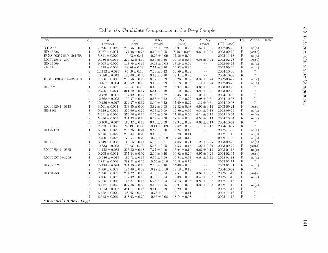
5.3D
etectedC
andid
ateC
ompan
ions
141
Table 5.6: Candidate Companions in the Deep Sample
Star NC ρ θ ∆KS KS J −KS t0 Tel. Assoc. Ref.(arcsec) (deg) (mag) (mag) (mag) (UT Date)
QT And 1 7.696 ± 0.019 239.56 ± 0.22 11.56 ± 0.22 18.91 ± 0.22 1.57 ± 0.31 2002-08-29 P no(a)HD 15526 1 0.077 ± 0.004 177.96 ± 0.75 0.00 ± 0.05 8.76 ± 0.06 0.61 ± 0.08 2003-09-20 P yes(c)1RXS J025216.9+361658 1 5.811 ± 0.020 10.63 ± 0.41 10.26 ± 0.09 17.86 ± 0.09 · · · 2002-11-18 P no(a)RX J0258.4+2947 1 0.086 ± 0.011 220.82 ± 4.14 0.60 ± 0.30 10.15 ± 0.30 0.58 ± 0.42 2002-02-28 P yes(c)HD 19668 1 6.565 ± 0.020 148.98 ± 0.19 10.58 ± 0.03 17.28 ± 0.04 · · · 2002-08-27 P no(a)AP 93 1 4.135 ± 0.026 83.86 ± 0.23 7.57 ± 0.30 16.93 ± 0.30 · · · 2003-09-20 P no(a)
2 12.452 ± 0.021 64.09 ± 0.13 7.23 ± 0.32 16.59 ± 0.32 · · · 2004-10-03 P ?3 10.680 ± 0.043 126.00 ± 0.20 9.98 ± 0.20 19.34 ± 0.20 · · · 2004-10-08 K ?
1RXS J031907.4+393418 1 7.656 ± 0.030 286.56 ± 0.25 8.77 ± 0.09 18.26 ± 0.09 0.87 ± 0.24 2002-08-29 P no(a)2 10.157 ± 0.024 333.52 ± 0.18 9.69 ± 0.09 19.18 ± 0.09 1.14 ± 0.24 2002-08-29 P no(a)
HE 622 1 7.275 ± 0.017 48.24 ± 0.18 6.38 ± 0.22 15.97 ± 0.22 0.66 ± 0.31 2003-09-20 P ?2 9.756 ± 0.024 311.79 ± 0.17 6.51 ± 0.22 16.10 ± 0.22 0.83 ± 0.31 2003-09-20 P ?3 12.478 ± 0.021 107.92 ± 0.12 8.76 ± 0.22 18.35 ± 0.22 1.03 ± 0.31 2004-10-08 K ?4 12.368 ± 0.023 109.57 ± 0.12 9.58 ± 0.22 19.17 ± 0.22 0.98 ± 0.31 2004-10-08 K ?5 10.436 ± 0.017 224.37 ± 0.12 8.10 ± 0.22 17.69 ± 0.22 1.12 ± 0.31 2004-10-08 K ?
RX J0329.1+0118 1 3.761 ± 0.004 303.35 ± 0.09 3.62 ± 0.08 12.82 ± 0.08 0.90 ± 0.14 2003-09-21 P yes(c)HE 1101 1 5.828 ± 0.025 323.66 ± 0.25 6.58 ± 0.09 15.89 ± 0.09 0.34 ± 0.13 2003-09-20 P no(a)
2 5.911 ± 0.010 276.86 ± 0.12 8.25 ± 0.09 17.56 ± 0.09 0.14 ± 0.13 2004-10-07 K no(c)3 5.316 ± 0.009 247.23 ± 0.12 9.13 ± 0.09 18.44 ± 0.09 0.53 ± 0.13 2004-10-07 K no(c)4 10.100 ± 0.017 113.32 ± 0.12 9.63 ± 0.09 18.94 ± 0.09 0.61 ± 0.13 2004-10-07 K ?5 2.173 ± 0.006 29.19 ± 0.14 10.11 ± 0.09 19.42 ± 0.09 1.15 ± 0.17 2004-10-07 K ?
HD 22179 1 6.536 ± 0.029 236.26 ± 0.24 8.82 ± 0.10 16.24 ± 0.10 · · · 2002-11-09 P no(a)2 6.616 ± 0.029 235.44 ± 0.23 9.30 ± 0.11 16.73 ± 0.11 · · · 2002-11-16 P no(a)3 9.200 ± 0.027 179.64 ± 0.23 10.20 ± 0.12 17.62 ± 0.12 · · · 2002-11-09 P no(a)
HII 120 1 3.549 ± 0.008 119.15 ± 0.14 5.75 ± 0.21 14.85 ± 0.21 1.21 ± 0.25 2003-09-20 P no(a)2 10.633 ± 0.023 70.53 ± 0.13 5.43 ± 0.15 14.53 ± 0.15 1.22 ± 0.20 2003-09-20 P yes(a)
RX J0354.4+0535 1 11.128 ± 0.035 225.82 ± 0.18 7.27 ± 0.10 15.94 ± 0.10 0.62 ± 0.18 2003-01-13 P no(c)2 0.205 ± 0.004 357.44 ± 0.92 2.10 ± 0.20 10.92 ± 0.20 0.97 ± 0.28 2004-02-07 P yes(c)
RX J0357.3+1258 1 10.086 ± 0.025 115.72 ± 0.19 6.56 ± 0.08 15.54 ± 0.08 0.64 ± 0.22 2003-01-11 P no(a)2 3.831 ± 0.026 338.31 ± 0.26 10.50 ± 0.10 19.48 ± 0.10 · · · 2003-01-11 P ?
HD 286179 1 10.124 ± 0.024 237.40 ± 0.19 7.20 ± 0.20 15.66 ± 0.20 · · · 2002-01-31 P no(a)2 3.406 ± 0.009 194.68 ± 0.22 10.72 ± 0.18 19.18 ± 0.18 · · · 2004-10-07 K ?
HD 31950 1 2.596 ± 0.007 264.22 ± 0.18 4.13 ± 0.04 12.51 ± 0.05 0.67 ± 0.07 2002-11-16 P yes(a)2 3.106 ± 0.007 137.92 ± 0.18 3.70 ± 0.04 12.08 ± 0.05 0.49 ± 0.07 2002-11-16 P no(c)3 6.925 ± 0.016 146.81 ± 0.18 6.35 ± 0.04 14.73 ± 0.05 0.89 ± 0.07 2002-11-16 P ?4 3.117 ± 0.015 327.86 ± 0.35 8.53 ± 0.05 16.91 ± 0.06 0.31 ± 0.08 2002-11-16 P no(c)5 10.013 ± 0.027 351.17 ± 0.16 9.91 ± 0.09 18.29 ± 0.09 · · · 2002-11-16 P ?6 6.528 ± 0.020 28.55 ± 0.14 10.73 ± 0.11 19.11 ± 0.11 · · · 2002-11-16 P ?7 6.313 ± 0.019 248.03 ± 0.20 10.36 ± 0.08 18.74 ± 0.08 · · · 2002-11-16 P ?
continued on next page

5.3D
etectedC
andid
ateC
ompan
ions
142Table 5.6–continued from previous page
Star NC ρ θ ∆KS KS J −KS t0 Tel. Assoc. Ref.(arcsec) (deg) (mag) (mag) (mag) (UT Date)
HD 36869 1 8.230 ± 0.014 152.30 ± 0.12 3.10 ± 0.35 9.95 ± 0.35 0.93 ± 0.35 2003-01-14 P yes(a)2 8.043 ± 0.016 249.72 ± 0.20 7.59 ± 0.15 14.44 ± 0.15 · · · 2003-01-14 P ?
1RXS J053650.0+133756 1 1.839 ± 0.018 37.26 ± 0.54 8.88 ± 0.30 16.95 ± 0.30 · · · 2002-02-28 P no(a)2 12.096 ± 0.027 212.16 ± 0.17 8.10 ± 0.10 16.17 ± 0.10 · · · 2002-02-28 P no(a)
HD 245567 1 0.348 ± 0.002 330.66 ± 0.23 1.79 ± 0.04 9.57 ± 0.04 0.52 ± 0.08 2002-11-16 P yes(c)2 3.185 ± 0.007 198.88 ± 0.17 6.44 ± 0.24 14.03 ± 0.24 0.54 ± 0.34 2002-11-16 P no(a)3 6.748 ± 0.024 316.18 ± 0.22 8.28 ± 0.24 15.87 ± 0.24 0.97 ± 0.34 2002-11-16 P no(a)4 10.927 ± 0.024 315.63 ± 0.17 6.21 ± 0.24 13.80 ± 0.24 0.55 ± 0.34 2002-11-16 P no(a)5 2.724 ± 0.007 21.87 ± 0.13 11.55 ± 0.24 19.14 ± 0.24 · · · 2003-11-09 K no(a)
SAO 150676 1 8.375 ± 0.029 351.31 ± 0.14 9.30 ± 0.20 16.77 ± 0.20 · · · 2002-11-17 P no(a)HD 49197 1 6.952 ± 0.016 345.82 ± 0.18 6.75 ± 0.06 12.82 ± 0.06 0.15 ± 0.12 2002-02-28 P no(a)
2 0.948 ± 0.032 77.50 ± 1.03 8.22 ± 0.14 14.29 ± 0.14 1.63 ± 1.21 2002-02-28 P yes(a)RE J0723+20 1 8.196 ± 0.013 80.86 ± 0.03 7.80 ± 0.20 14.68 ± 0.20 0.16 ± 0.22 2002-02-28 P no(a)
2 5.532 ± 0.013 329.36 ± 0.09 8.40 ± 0.20 15.28 ± 0.20 1.06 ± 0.22 2002-02-28 P no(a)HD 60737 1 7.657 ± 0.029 127.25 ± 0.18 9.40 ± 0.20 15.65 ± 0.20 · · · 2002-01-31 P no(a)HD 70573 1 1.050 ± 0.066 294.24 ± 3.17 9.07 ± 0.15 16.26 ± 0.15 · · · 2002-02-01 P ?HD 82443 1 5.459 ± 0.010 190.30 ± 0.23 11.77 ± 0.14 16.89 ± 0.14 · · · 2004-02-07 P ?
2 8.154 ± 0.020 98.76 ± 0.15 12.59 ± 0.21 17.71 ± 0.21 · · · 2004-02-07 P ?3 7.142 ± 0.027 253.71 ± 0.23 13.84 ± 0.30 18.96 ± 0.30 · · · 2004-02-07 P ?
SAO 178272 1 10.082 ± 0.032 356.64 ± 0.18 9.67 ± 0.15 17.06 ± 0.15 · · · 2003-01-13 P ?2 8.184 ± 0.046 274.53 ± 0.15 10.75 ± 0.22 18.14 ± 0.22 · · · 2003-01-13 P ?
HD 90905 1 5.816 ± 0.027 191.77 ± 0.23 11.30 ± 0.10 16.82 ± 0.10 · · · 2002-02-01 P no(a)2 12.446 ± 0.031 176.73 ± 0.13 13.49 ± 0.19 19.01 ± 0.19 · · · 2004-06-05 K no(e)
HD 91782 1 1.002 ± 0.008 33.67 ± 0.46 4.30 ± 0.06 11.08 ± 0.06 0.90 ± 0.13 2002-03-02 P yes(a)HD 92855 1 2.934 ± 0.005 291.33 ± 0.13 4.57 ± 0.09 10.46 ± 0.09 0.75 ± 0.15 2002-02-01 P yes(a) FM00
2 12.216 ± 0.022 147.79 ± 0.25 8.90 ± 0.20 14.79 ± 0.20 · · · 2002-02-01 P no(a)BPM 87617 1 0.248 ± 0.002 273.22 ± 0.11 0.13 ± 0.06 8.58 ± 0.06 1.02 ± 0.08 2003-01-12 P yes(a)
2 10.038 ± 0.009 325.65 ± 0.09 6.40 ± 0.06 14.16 ± 0.06 0.13 ± 0.09 2003-01-12 P no(a)HD 104576 1 10.455 ± 0.028 19.66 ± 0.21 11.00 ± 0.50 17.68 ± 0.50 · · · 2002-06-22 P no(e)HD 104860 1 3.803 ± 0.027 287.01 ± 0.28 10.92 ± 0.25 17.42 ± 0.25 0.00 ± 0.47 2002-06-23 P no(a)
2 11.961 ± 0.033 260.09 ± 0.19 12.09 ± 0.18 18.59 ± 0.18 · · · 2004-06-05 K no(e)SAO 15880 1 2.176 ± 0.018 293.93 ± 0.72 8.98 ± 0.17 16.27 ± 0.17 · · · 2004-02-06 P no(a)HD 111456 1 3.783 ± 0.010 117.45 ± 0.30 12.72 ± 0.16 17.27 ± 0.16 · · · 2004-02-06 P ?HD 139498 1 0.311 ± 0.002 3.39 ± 0.21 0.00 ± 0.02 8.26 ± 0.03 0.50 ± 0.05 2003-07-15 P yes(a)
2 11.246 ± 0.033 123.98 ± 0.19 8.48 ± 0.30 15.98 ± 0.30 · · · 2004-06-26 P ?3 8.801 ± 0.026 61.50 ± 0.21 10.98 ± 0.30 18.49 ± 0.30 · · · 2004-06-26 P ?
HD 142361 1 0.705 ± 0.001 236.41 ± 0.13 2.01 ± 0.10 9.19 ± 0.10 0.85 ± 0.14 2002-06-21 P yes(a)2 11.207 ± 0.046 164.99 ± 0.17 5.85 ± 0.17 12.88 ± 0.17 0.77 ± 0.28 2002-06-21 P no(a)
HD 143006 1 8.355 ± 0.026 130.27 ± 0.25 9.28 ± 0.16 16.33 ± 0.16 1.18 ± 0.23 2002-06-23 P ?2 6.626 ± 0.028 0.32 ± 0.23 10.40 ± 0.16 17.45 ± 0.16 1.40 ± 0.23 2002-06-23 P ?3 8.502 ± 0.029 268.41 ± 0.23 10.66 ± 0.16 17.71 ± 0.16 1.27 ± 0.23 2002-06-23 P no(a)4 7.698 ± 0.023 357.97 ± 0.12 12.11 ± 0.16 19.16 ± 0.16 1.30 ± 0.23 2003-05-18 K ?5 12.279 ± 0.028 102.74 ± 0.12 11.29 ± 0.16 18.34 ± 0.16 0.88 ± 0.23 2003-05-18 K ?
(PZ99) J155847.8–175800 1 9.118 ± 0.034 224.72 ± 0.35 11.25 ± 0.22 19.58 ± 0.22 · · · 2004-06-06 K ?ScoPMS 21 1 6.221 ± 0.014 36.94 ± 0.13 7.39 ± 0.02 15.91 ± 0.03 1.05 ± 0.05 2002-06-22 P no(a)
2 9.888 ± 0.027 74.26 ± 0.18 8.06 ± 0.04 16.58 ± 0.05 0.67 ± 0.06 2002-06-22 P no(c)
continued on next page

5.3D
etectedC
andid
ateC
ompan
ions
143Table 5.6–continued from previous page
Star NC ρ θ ∆KS KS J −KS t0 Tel. Assoc. Ref.(arcsec) (deg) (mag) (mag) (mag) (UT Date)
3 9.351 ± 0.020 308.13 ± 0.16 8.93 ± 0.02 17.45 ± 0.03 1.11 ± 0.08 2002-06-22 P no(a)(PZ99) J160302.7–180605 1 1.572 ± 0.006 190.97 ± 0.19 9.59 ± 0.09 18.32 ± 0.09 2.42 ± 0.17 2003-05-18 K no(a)
2 5.797 ± 0.013 272.51 ± 0.13 7.58 ± 0.62 16.31 ± 0.62 · · · 2003-05-18 K no(a)3 9.065 ± 0.020 73.35 ± 0.12 10.58 ± 0.49 19.31 ± 0.49 · · · 2003-05-18 K ?4 9.653 ± 0.023 107.18 ± 0.12 11.81 ± 0.53 20.54 ± 0.53 · · · 2003-05-18 K ?
ScoPMS 27 1 0.079 ± 0.006 77.04 ± 0.77 0.60 ± 0.20 9.14 ± 0.20 0.83 ± 0.28 2004-06-28 P yes(c)2 11.113 ± 0.025 218.10 ± 0.22 10.33 ± 0.30 18.37 ± 0.30 · · · 2004-06-28 P no(a)3 5.807 ± 0.027 87.35 ± 0.20 10.59 ± 0.30 18.63 ± 0.30 · · · 2004-06-28 P ?4 5.346 ± 0.026 336.58 ± 0.21 10.47 ± 0.30 18.51 ± 0.30 · · · 2004-06-28 P ?
ScoPMS 52 1 0.144 ± 0.005 162.15 ± 1.76 1.10 ± 0.10 8.93 ± 0.10 · · · 2002-08-31 P yes(a) G93(PZ99) J161318.6–221248 1 3.770 ± 0.012 313.46 ± 0.22 11.00 ± 0.10 18.43 ± 0.10 · · · 2002-06-21 P no(a)
2 3.333 ± 0.021 81.19 ± 0.41 11.20 ± 0.10 18.63 ± 0.10 · · · 2002-06-21 P no(a)3 8.860 ± 0.034 77.36 ± 0.23 11.00 ± 0.20 18.43 ± 0.20 · · · 2002-06-21 P no(a)4 7.957 ± 0.018 152.07 ± 0.13 10.83 ± 0.22 18.26 ± 0.22 · · · 2003-05-18 K ?5 12.182 ± 0.029 259.12 ± 0.17 10.72 ± 0.21 18.15 ± 0.21 · · · 2003-05-18 K ?
(PZ99) J161402.1–230101 1 5.366 ± 0.030 356.14 ± 0.49 7.76 ± 0.12 16.37 ± 0.12 · · · 2003-07-15 P ?2 9.633 ± 0.015 128.34 ± 0.15 9.16 ± 0.17 17.77 ± 0.17 · · · 2004-06-05 K ?3 7.858 ± 0.017 281.13 ± 0.13 10.35 ± 0.17 18.96 ± 0.17 · · · 2004-06-05 K ?
(PZ99) J161411.0–230536 1 0.222 ± 0.003 304.76 ± 0.41 0.21 ± 0.10 8.32 ± 0.10 0.84 ± 0.18 2002-06-21 P yes(a)2 2.659 ± 0.007 100.46 ± 0.21 6.26 ± 0.03 13.72 ± 0.04 0.82 ± 0.11 2002-06-21 P no(a)3 2.808 ± 0.010 98.36 ± 0.14 10.25 ± 0.50 18.73 ± 0.50 · · · 2004-06-05 K ?4 7.709 ± 0.017 341.92 ± 0.12 8.16 ± 0.10 15.62 ± 0.10 0.33 ± 0.22 2004-06-05 K no(c)5 8.037 ± 0.018 145.10 ± 0.12 9.50 ± 0.06 16.96 ± 0.07 · · · 2004-06-05 K ?6 8.926 ± 0.021 80.29 ± 0.12 11.72 ± 0.17 19.18 ± 0.17 · · · 2004-06-05 K ?7 9.243 ± 0.021 69.00 ± 0.15 12.51 ± 0.20 19.97 ± 0.20 · · · 2004-06-05 K ?
(PZ99) J161459.2–275023 1 4.787 ± 0.025 264.80 ± 0.20 7.07 ± 0.15 15.76 ± 0.15 · · · 2003-07-15 P ?2 5.554 ± 0.072 187.48 ± 0.58 7.40 ± 0.15 16.09 ± 0.15 · · · 2003-07-15 P ?3 3.919 ± 0.010 153.63 ± 0.13 9.65 ± 0.17 18.34 ± 0.17 · · · 2004-06-05 K ?4 12.299 ± 0.027 253.55 ± 0.12 8.89 ± 0.18 17.58 ± 0.18 · · · 2004-06-05 K ?5 11.464 ± 0.026 72.94 ± 0.12 9.91 ± 0.17 18.60 ± 0.17 · · · 2004-06-05 K ?6 6.241 ± 0.015 259.72 ± 0.17 10.65 ± 0.18 19.34 ± 0.18 · · · 2004-06-05 K ?7 7.936 ± 0.018 55.55 ± 0.14 10.59 ± 0.19 19.28 ± 0.19 · · · 2004-06-05 K ?
(PZ99) J161618.0–233947 1 9.119 ± 0.028 160.44 ± 0.06 7.26 ± 0.30 15.36 ± 0.30 · · · 2004-06-27 P ?2 10.049 ± 0.026 195.43 ± 0.06 7.57 ± 0.13 15.67 ± 0.13 · · · 2004-06-27 P ?3 3.190 ± 0.015 184.47 ± 0.64 10.44 ± 0.15 18.54 ± 0.15 · · · 2004-06-27 P ?4 10.938 ± 0.021 165.25 ± 0.18 10.03 ± 0.11 18.13 ± 0.11 · · · 2004-06-27 P ?5 12.451 ± 0.020 251.52 ± 0.20 9.31 ± 0.18 17.41 ± 0.18 · · · 2004-06-27 P ?6 3.671 ± 0.025 140.63 ± 0.22 10.81 ± 0.30 18.91 ± 0.30 · · · 2004-06-27 P ?7 6.845 ± 0.025 144.15 ± 0.22 10.70 ± 0.30 18.80 ± 0.30 · · · 2004-06-27 P ?8 9.452 ± 0.028 108.96 ± 0.21 10.68 ± 0.30 18.78 ± 0.30 · · · 2004-06-27 P ?9 12.309 ± 0.025 38.57 ± 0.22 10.51 ± 0.30 18.61 ± 0.30 · · · 2004-06-27 P ?10 3.711 ± 0.026 184.89 ± 0.20 11.43 ± 0.30 19.53 ± 0.30 · · · 2004-06-27 P ?
HD 146516 1 5.738 ± 0.012 222.79 ± 0.13 7.60 ± 0.09 15.57 ± 0.09 0.80 ± 0.15 2003-05-10 P no(a)2 9.218 ± 0.028 333.77 ± 0.14 7.50 ± 0.09 15.47 ± 0.09 0.74 ± 0.15 2003-05-10 P ?3 9.493 ± 0.021 81.79 ± 0.12 10.40 ± 0.18 18.37 ± 0.18 · · · 2004-06-05 K ?4 6.256 ± 0.020 350.00 ± 0.13 11.67 ± 0.23 19.64 ± 0.23 · · · 2004-06-05 K ?
continued on next page
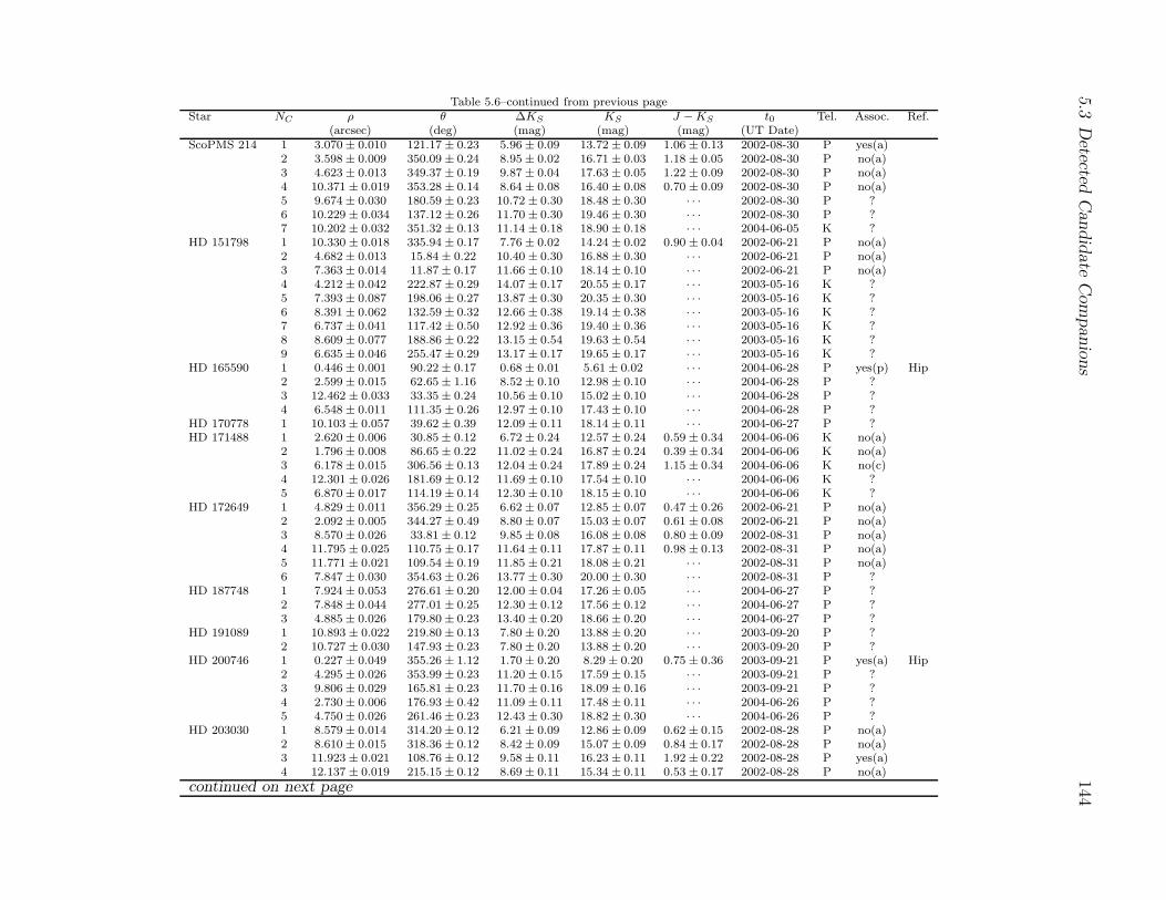
5.3D
etectedC
andid
ateC
ompan
ions
144Table 5.6–continued from previous page
Star NC ρ θ ∆KS KS J −KS t0 Tel. Assoc. Ref.(arcsec) (deg) (mag) (mag) (mag) (UT Date)
ScoPMS 214 1 3.070 ± 0.010 121.17 ± 0.23 5.96 ± 0.09 13.72 ± 0.09 1.06 ± 0.13 2002-08-30 P yes(a)2 3.598 ± 0.009 350.09 ± 0.24 8.95 ± 0.02 16.71 ± 0.03 1.18 ± 0.05 2002-08-30 P no(a)3 4.623 ± 0.013 349.37 ± 0.19 9.87 ± 0.04 17.63 ± 0.05 1.22 ± 0.09 2002-08-30 P no(a)4 10.371 ± 0.019 353.28 ± 0.14 8.64 ± 0.08 16.40 ± 0.08 0.70 ± 0.09 2002-08-30 P no(a)5 9.674 ± 0.030 180.59 ± 0.23 10.72 ± 0.30 18.48 ± 0.30 · · · 2002-08-30 P ?6 10.229 ± 0.034 137.12 ± 0.26 11.70 ± 0.30 19.46 ± 0.30 · · · 2002-08-30 P ?7 10.202 ± 0.032 351.32 ± 0.13 11.14 ± 0.18 18.90 ± 0.18 · · · 2004-06-05 K ?
HD 151798 1 10.330 ± 0.018 335.94 ± 0.17 7.76 ± 0.02 14.24 ± 0.02 0.90 ± 0.04 2002-06-21 P no(a)2 4.682 ± 0.013 15.84 ± 0.22 10.40 ± 0.30 16.88 ± 0.30 · · · 2002-06-21 P no(a)3 7.363 ± 0.014 11.87 ± 0.17 11.66 ± 0.10 18.14 ± 0.10 · · · 2002-06-21 P no(a)4 4.212 ± 0.042 222.87 ± 0.29 14.07 ± 0.17 20.55 ± 0.17 · · · 2003-05-16 K ?5 7.393 ± 0.087 198.06 ± 0.27 13.87 ± 0.30 20.35 ± 0.30 · · · 2003-05-16 K ?6 8.391 ± 0.062 132.59 ± 0.32 12.66 ± 0.38 19.14 ± 0.38 · · · 2003-05-16 K ?7 6.737 ± 0.041 117.42 ± 0.50 12.92 ± 0.36 19.40 ± 0.36 · · · 2003-05-16 K ?8 8.609 ± 0.077 188.86 ± 0.22 13.15 ± 0.54 19.63 ± 0.54 · · · 2003-05-16 K ?9 6.635 ± 0.046 255.47 ± 0.29 13.17 ± 0.17 19.65 ± 0.17 · · · 2003-05-16 K ?
HD 165590 1 0.446 ± 0.001 90.22 ± 0.17 0.68 ± 0.01 5.61 ± 0.02 · · · 2004-06-28 P yes(p) Hip2 2.599 ± 0.015 62.65 ± 1.16 8.52 ± 0.10 12.98 ± 0.10 · · · 2004-06-28 P ?3 12.462 ± 0.033 33.35 ± 0.24 10.56 ± 0.10 15.02 ± 0.10 · · · 2004-06-28 P ?4 6.548 ± 0.011 111.35 ± 0.26 12.97 ± 0.10 17.43 ± 0.10 · · · 2004-06-28 P ?
HD 170778 1 10.103 ± 0.057 39.62 ± 0.39 12.09 ± 0.11 18.14 ± 0.11 · · · 2004-06-27 P ?HD 171488 1 2.620 ± 0.006 30.85 ± 0.12 6.72 ± 0.24 12.57 ± 0.24 0.59 ± 0.34 2004-06-06 K no(a)
2 1.796 ± 0.008 86.65 ± 0.22 11.02 ± 0.24 16.87 ± 0.24 0.39 ± 0.34 2004-06-06 K no(a)3 6.178 ± 0.015 306.56 ± 0.13 12.04 ± 0.24 17.89 ± 0.24 1.15 ± 0.34 2004-06-06 K no(c)4 12.301 ± 0.026 181.69 ± 0.12 11.69 ± 0.10 17.54 ± 0.10 · · · 2004-06-06 K ?5 6.870 ± 0.017 114.19 ± 0.14 12.30 ± 0.10 18.15 ± 0.10 · · · 2004-06-06 K ?
HD 172649 1 4.829 ± 0.011 356.29 ± 0.25 6.62 ± 0.07 12.85 ± 0.07 0.47 ± 0.26 2002-06-21 P no(a)2 2.092 ± 0.005 344.27 ± 0.49 8.80 ± 0.07 15.03 ± 0.07 0.61 ± 0.08 2002-06-21 P no(a)3 8.570 ± 0.026 33.81 ± 0.12 9.85 ± 0.08 16.08 ± 0.08 0.80 ± 0.09 2002-08-31 P no(a)4 11.795 ± 0.025 110.75 ± 0.17 11.64 ± 0.11 17.87 ± 0.11 0.98 ± 0.13 2002-08-31 P no(a)5 11.771 ± 0.021 109.54 ± 0.19 11.85 ± 0.21 18.08 ± 0.21 · · · 2002-08-31 P no(a)6 7.847 ± 0.030 354.63 ± 0.26 13.77 ± 0.30 20.00 ± 0.30 · · · 2002-08-31 P ?
HD 187748 1 7.924 ± 0.053 276.61 ± 0.20 12.00 ± 0.04 17.26 ± 0.05 · · · 2004-06-27 P ?2 7.848 ± 0.044 277.01 ± 0.25 12.30 ± 0.12 17.56 ± 0.12 · · · 2004-06-27 P ?3 4.885 ± 0.026 179.80 ± 0.23 13.40 ± 0.20 18.66 ± 0.20 · · · 2004-06-27 P ?
HD 191089 1 10.893 ± 0.022 219.80 ± 0.13 7.80 ± 0.20 13.88 ± 0.20 · · · 2003-09-20 P ?2 10.727 ± 0.030 147.93 ± 0.23 7.80 ± 0.20 13.88 ± 0.20 · · · 2003-09-20 P ?
HD 200746 1 0.227 ± 0.049 355.26 ± 1.12 1.70 ± 0.20 8.29 ± 0.20 0.75 ± 0.36 2003-09-21 P yes(a) Hip2 4.295 ± 0.026 353.99 ± 0.23 11.20 ± 0.15 17.59 ± 0.15 · · · 2003-09-21 P ?3 9.806 ± 0.029 165.81 ± 0.23 11.70 ± 0.16 18.09 ± 0.16 · · · 2003-09-21 P ?4 2.730 ± 0.006 176.93 ± 0.42 11.09 ± 0.11 17.48 ± 0.11 · · · 2004-06-26 P ?5 4.750 ± 0.026 261.46 ± 0.23 12.43 ± 0.30 18.82 ± 0.30 · · · 2004-06-26 P ?
HD 203030 1 8.579 ± 0.014 314.20 ± 0.12 6.21 ± 0.09 12.86 ± 0.09 0.62 ± 0.15 2002-08-28 P no(a)2 8.610 ± 0.015 318.36 ± 0.12 8.42 ± 0.09 15.07 ± 0.09 0.84 ± 0.17 2002-08-28 P no(a)3 11.923 ± 0.021 108.76 ± 0.12 9.58 ± 0.11 16.23 ± 0.11 1.92 ± 0.22 2002-08-28 P yes(a)4 12.137 ± 0.019 215.15 ± 0.12 8.69 ± 0.11 15.34 ± 0.11 0.53 ± 0.17 2002-08-28 P no(a)
continued on next page

5.3D
etectedC
andid
ateC
ompan
ions
145Table 5.6–continued from previous page
Star NC ρ θ ∆KS KS J −KS t0 Tel. Assoc. Ref.(arcsec) (deg) (mag) (mag) (mag) (UT Date)
5 9.933 ± 0.027 218.43 ± 0.20 11.29 ± 0.08 17.94 ± 0.08 · · · 2002-08-28 P no(a)6 3.365 ± 0.025 343.13 ± 0.23 11.76 ± 0.30 18.41 ± 0.30 · · · 2002-08-28 P no(a)
HD 209393 1 9.187 ± 0.018 6.57 ± 0.13 10.81 ± 0.10 17.13 ± 0.10 · · · 2002-11-17 P no(a)2 8.188 ± 0.017 71.50 ± 0.14 12.80 ± 0.20 19.12 ± 0.20 · · · 2002-11-17 P no(a)3 6.237 ± 0.013 317.66 ± 0.18 13.11 ± 0.22 19.43 ± 0.22 · · · 2002-11-17 P no(a)4 10.344 ± 0.025 210.77 ± 0.15 12.83 ± 0.11 19.15 ± 0.11 · · · 2002-11-17 P no(a)
V383 Lac 1 10.736 ± 0.020 91.89 ± 0.16 8.74 ± 0.04 15.24 ± 0.05 · · · 2002-08-27 P no(a)2 11.744 ± 0.024 140.12 ± 0.14 11.12 ± 0.09 17.62 ± 0.09 · · · 2002-08-27 P no(a)3 9.240 ± 0.017 108.35 ± 0.18 10.97 ± 0.08 17.47 ± 0.08 · · · 2002-08-27 P no(a)4 4.427 ± 0.018 200.35 ± 0.16 11.10 ± 0.12 17.61 ± 0.12 · · · 2002-08-27 P no(a)5 4.231 ± 0.010 98.09 ± 0.56 11.57 ± 0.11 18.08 ± 0.11 · · · 2002-08-27 P no(a)6 11.594 ± 0.025 270.42 ± 0.13 11.44 ± 0.10 17.94 ± 0.10 · · · 2002-08-27 P no(a)
HD 218738 1 10.619 ± 0.026 97.59 ± 0.17 8.10 ± 1.00 13.76 ± 1.00 · · · 2003-12-10 P no(a)2 10.616 ± 0.025 97.81 ± 0.18 8.07 ± 1.00 13.73 ± 1.00 · · · 2003-12-10 P no(a)3 4.144 ± 0.014 182.07 ± 0.23 10.09 ± 0.23 15.75 ± 0.23 · · · 2003-12-10 P no(a)4 5.339 ± 0.016 120.60 ± 0.17 11.83 ± 0.27 17.49 ± 0.27 · · · 2003-12-10 P no(a)5 6.022 ± 0.022 38.28 ± 0.25 12.68 ± 0.25 18.34 ± 0.25 · · · 2003-12-10 P no(a)6 5.508 ± 0.028 33.36 ± 0.26 13.70 ± 0.50 19.36 ± 0.50 · · · 2003-12-10 P no(a)7 9.186 ± 0.032 42.22 ± 0.26 13.58 ± 0.30 19.24 ± 0.30 · · · 2003-12-10 P ?8 2.134 ± 0.018 224.02 ± 0.33 10.96 ± 0.50 16.62 ± 0.50 · · · 2004-10-04 P no(a)
HD 218739 1 7.050 ± 0.030 221.73 ± 0.34 7.45 ± 0.50 13.12 ± 0.50 · · · 2003-12-10 P no(a)2 12.055 ± 0.055 238.54 ± 0.34 12.78 ± 0.30 18.45 ± 0.30 · · · 2003-12-10 P no(a)3 9.526 ± 0.039 287.92 ± 0.34 13.16 ± 0.50 18.83 ± 0.50 · · · 2003-12-10 P no(a)
HD 219498 1 8.862 ± 0.022 129.85 ± 0.19 8.69 ± 0.14 16.07 ± 0.14 · · · 2002-08-30 P no(a)2 9.792 ± 0.032 305.61 ± 0.25 11.76 ± 0.07 19.14 ± 0.07 · · · 2002-08-30 P no(a)
References.— FM00: Fabricius & Makarov (2000); G93: Ghez et al. (1993); Hip: Perryman et al. (1997, Hipparcos).

5.3D
etectedC
andid
ateC
ompan
ions
146
Table 5.7: Candidate Companions in the Shallow SampleStar N ρ θ ∆KS KS J −KS t0 Tel. Assoc. Ref.
(arcsec) (deg) (mag) (mag) (mag) (UT Date)HD 224873 1 1.268 ± 0.002 171.44 ± 0.12 0.25 ± 0.02 7.57 ± 0.03 0.50 ± 0.05 2002-08-31 P yes(a)HD 9472 1 2.793 ± 0.025 343.69 ± 0.30 5.79 ± 0.09 11.83 ± 0.09 1.04 ± 0.14 2002-11-18 P yes(a)RE J0137+18A 1 1.691 ± 0.006 24.60 ± 0.12 0.05 ± 0.01 7.49 ± 0.02 0.76 ± 0.03 2002-01-31 P yes(a)HD 13531 1 0.717 ± 0.003 16.79 ± 0.43 4.20 ± 0.08 9.88 ± 0.08 1.04 ± 0.15 2002-08-28 P yes(a)1RXS J025223.5+372914 1 0.637 ± 0.003 91.28 ± 0.28 1.43 ± 0.08 10.77 ± 0.08 0.67 ± 0.12 2003-09-21 P yes(a)
2 5.255 ± 0.016 76.85 ± 0.18 4.37 ± 0.09 13.45 ± 0.09 0.50 ± 0.13 2003-09-21 P no(a)2RE J0255+474 1 2.131 ± 0.004 272.63 ± 0.16 0.08 ± 0.05 7.29 ± 0.06 0.72 ± 0.08 2002-02-28 P yes(a) WDS
2 11.469 ± 0.033 46.40 ± 0.11 7.00 ± 0.10 14.21 ± 0.10 0.57 ± 0.14 2002-02-28 P no(a)HD 18940 1 0.167 ± 0.002 8.59 ± 1.18 0.78 ± 0.03 6.71 ± 0.04 0.51 ± 0.08 2002-08-29 P yes(c)
2 4.321 ± 0.012 207.38 ± 0.12 4.58 ± 0.03 10.08 ± 0.04 0.92 ± 0.07 2002-08-29 P ?3 4.120 ± 0.010 203.78 ± 0.13 5.21 ± 0.03 10.71 ± 0.04 0.81 ± 0.07 2002-08-29 P ?
vB 1 1 2.470 ± 0.006 200.63 ± 0.14 2.63 ± 0.03 8.62 ± 0.04 0.91 ± 0.06 2002-08-29 P yes(c)HE 350 1 8.464 ± 0.016 109.22 ± 0.14 5.85 ± 0.21 15.11 ± 0.21 1.50 ± 0.37 2003-09-20 P no(a)
2 6.896 ± 0.011 38.37 ± 0.19 7.66 ± 0.30 16.92 ± 0.30 · · · 2004-10-04 P ?HE 373 1 2.081 ± 0.005 193.77 ± 0.18 5.24 ± 0.10 14.59 ± 0.10 0.98 ± 0.14 2003-09-20 P yes(a)
2 11.598 ± 0.031 265.81 ± 0.25 7.51 ± 0.30 16.86 ± 0.30 · · · 2003-09-20 P ?3 8.478 ± 0.034 55.82 ± 0.22 8.37 ± 0.30 17.72 ± 0.30 · · · 2003-09-20 P ?
HE 389 1 9.023 ± 0.016 133.30 ± 0.12 5.47 ± 0.13 14.96 ± 0.13 1.10 ± 0.18 2003-09-20 P no(a)HE 696 1 0.448 ± 0.001 357.22 ± 0.18 2.72 ± 0.08 12.50 ± 0.08 0.70 ± 0.12 2003-09-20 P yes(a) P02HE 935 1 0.026 ± 0.025 247.44 ± 0.21 0.00 ± 0.20 9.21 ± 0.20 0.40 ± 0.28 2003-09-20 P yes(c) P02
2 3.116 ± 0.025 109.45 ± 0.21 8.70 ± 0.30 17.16 ± 0.30 · · · 2003-09-20 P ?HII 102 1 3.599 ± 0.009 213.29 ± 0.14 3.07 ± 0.10 11.72 ± 0.10 1.05 ± 0.14 2003-09-20 P yes(a) B97
2 9.959 ± 0.027 240.21 ± 0.16 5.75 ± 0.10 14.40 ± 0.10 1.05 ± 0.14 2003-09-20 P ?1RXS J034423.3+281224 1 0.425 ± 0.002 202.20 ± 0.10 1.13 ± 0.10 8.62 ± 0.10 0.48 ± 0.22 2002-11-17 P yes(a)
2 5.711 ± 0.006 313.30 ± 0.12 7.11 ± 0.11 14.27 ± 0.11 · · · 2004-10-05 P ?HII 571 1 3.903 ± 0.005 66.10 ± 0.08 3.84 ± 0.08 13.07 ± 0.08 0.95 ± 0.12 2003-12-10 P yes(a) B97,M92HII 1101 1 9.167 ± 0.016 104.93 ± 0.12 5.70 ± 0.09 14.46 ± 0.09 0.40 ± 0.16 2003-12-10 P no(a)HII 1182 1 1.113 ± 0.009 219.69 ± 0.26 4.54 ± 0.19 13.48 ± 0.19 · · · 2003-12-10 P yes(a) B97HII 1348 1 1.097 ± 0.003 346.79 ± 0.18 5.15 ± 0.09 14.88 ± 0.09 1.16 ± 0.13 2004-10-03 P yes(a)HII 2106 1 0.240 ± 0.010 31.09 ± 0.59 1.71 ± 0.12 11.29 ± 0.12 · · · 2003-12-10 P yes(a) B97RX J0348.9+0110 1 0.047 ± 0.007 41.50 ± 3.64 0.00 ± 0.05 9.02 ± 0.06 · · · 2003-12-10 P yes(a)HII 2278 1 0.331 ± 0.005 179.20 ± 0.32 0.03 ± 0.02 9.57 ± 0.03 · · · 2003-12-10 P yes(a) B97HII 2881 1 0.099 ± 0.005 335.73 ± 1.20 0.26 ± 0.09 9.94 ± 0.09 · · · 2003-12-10 P yes(a) B97HD 285281 1 0.770 ± 0.001 188.34 ± 0.05 1.20 ± 0.10 9.12 ± 0.10 0.66 ± 0.14 2002-02-01 P yes(a) KL98HD 284135 1 0.367 ± 0.002 253.23 ± 0.21 0.12 ± 0.01 8.58 ± 0.02 · · · 2002-01-31 P yes(a) WDSHD 281691 1 6.768 ± 0.014 138.91 ± 0.13 1.90 ± 0.05 10.30 ± 0.06 0.74 ± 0.08 2002-11-18 P yes(a) KL98HD 26182 1 0.818 ± 0.002 175.11 ± 0.11 0.92 ± 0.08 9.09 ± 0.08 0.42 ± 0.11 2003-12-10 P yes(c) WDSHD 284266 1 0.569 ± 0.006 356.92 ± 0.11 1.90 ± 0.10 10.66 ± 0.10 0.89 ± 0.41 2002-01-31 P yes(a) KL98HD 26990 1 0.123 ± 0.004 163.56 ± 1.40 0.38 ± 0.20 6.81 ± 0.20 0.67 ± 0.36 2003-12-10 P yes(a)vB 49 1 2.139 ± 0.017 256.86 ± 0.16 4.60 ± 0.14 11.40 ± 0.14 · · · 2003-01-12 P yes(c)vB 52 1 1.115 ± 0.002 236.40 ± 0.18 2.73 ± 0.06 9.10 ± 0.06 0.85 ± 0.08 2003-01-12 P yes(a) P98
continued on next page

5.3D
etectedC
andid
ateC
ompan
ions
147Table 5.7–continued from previous page
Star Comp. ρ θ ∆KS KS J −KS t0 Tel. Assoc. Ref.(arcsec) (deg) (mag) (mag) (mag) (UT Date)
vB 176 1 0.227 ± 0.003 307.06 ± 0.38 0.28 ± 0.09 7.67 ± 0.09 · · · 2003-12-10 P yes(a) HipvB 66 1 9.781 ± 0.023 248.88 ± 0.11 10.75 ± 0.10 16.91 ± 0.10 · · · 2002-11-17 P ?vB 91 1 0.133 ± 0.002 172.98 ± 2.79 0.37 ± 0.14 7.72 ± 0.14 · · · 2003-12-10 P yes(a)vB 96 1 0.171 ± 0.003 264.05 ± 0.78 0.36 ± 0.10 7.41 ± 0.10 · · · 2003-12-10 P yes(p) P98RX J0434.3+0226 1 1.340 ± 0.022 271.76 ± 0.30 2.38 ± 0.05 11.99 ± 0.06 0.77 ± 0.11 2003-01-12 P yes(c)vB 106 1 7.230 ± 0.012 76.50 ± 0.44 9.50 ± 0.30 15.94 ± 0.30 · · · 2003-12-10 P no(a)HD 282346 1 0.461 ± 0.001 272.14 ± 0.18 1.13 ± 0.04 8.91 ± 0.04 0.61 ± 0.17 2002-11-18 P yes(a) HipvB 142 1 6.070 ± 0.013 123.82 ± 0.16 11.30 ± 0.20 18.04 ± 0.20 · · · 2002-11-17 P no(a)1RXS J051111.1+281353 1 0.495 ± 0.001 211.51 ± 0.10 0.39 ± 0.04 8.77 ± 0.05 0.69 ± 0.07 2002-02-28 P yes(a)HD 61994 1 5.210 ± 0.008 77.00 ± 0.08 7.32 ± 0.13 12.67 ± 0.13 0.28 ± 0.30 2002-11-18 P no(c)HD 69076 1 1.232 ± 0.005 101.06 ± 0.11 3.91 ± 0.05 10.38 ± 0.05 1.04 ± 0.21 2002-11-18 P yes(a)HD 71974 1 0.383 ± 0.014 87.34 ± 0.63 0.42 ± 0.05 6.45 ± 0.06 0.35 ± 0.21 2002-03-03 P yes(c) S99HD 72760 1 0.964 ± 0.007 215.08 ± 0.38 4.84 ± 0.01 10.28 ± 0.02 1.01 ± 0.04 2002-11-16 P yes(c)HD 77407 1 1.659 ± 0.004 353.36 ± 0.04 2.00 ± 0.10 7.60 ± 0.10 0.90 ± 0.14 2002-01-31 P yes(a) M04HD 78899 1 8.174 ± 0.013 75.76 ± 0.12 3.36 ± 0.08 9.17 ± 0.08 0.79 ± 0.13 2003-12-09 P ?HD 91962 1 0.842 ± 0.003 176.00 ± 0.11 1.37 ± 0.06 7.03 ± 0.06 0.73 ± 0.13 2002-03-02 P yes(a)
2 0.142 ± 0.004 56.17 ± 1.76 1.25 ± 0.11 6.94 ± 0.11 0.98 ± 0.19 2003-05-10 P yes(c)HD 99565 1 0.408 ± 0.001 6.13 ± 0.18 0.09 ± 0.05 6.55 ± 0.05 0.48 ± 0.06 2003-01-11 P yes(a) WDSHD 108799 1 2.070 ± 0.006 338.46 ± 0.09 1.47 ± 0.02 6.30 ± 0.03 0.80 ± 0.06 2003-05-10 P yes(a)HD 108944 1 1.941 ± 0.006 345.48 ± 0.18 3.49 ± 0.02 9.56 ± 0.03 0.85 ± 0.09 2002-03-03 P yes(a)HD 112196 1 1.501 ± 0.001 55.52 ± 0.09 2.07 ± 0.01 7.77 ± 0.02 0.73 ± 0.04 2002-02-01 P yes(a)HD 115043 1 1.639 ± 0.003 358.61 ± 0.05 4.87 ± 0.08 10.22 ± 0.08 0.86 ± 0.12 2003-12-09 P yes(a) L05HD 129333 1 0.717 ± 0.009 172.77 ± 0.11 2.83 ± 0.05 8.82 ± 0.05 0.81 ± 0.07 2003-01-11 P yes(a) DM91,MH04HD 134319 1 5.356 ± 0.020 260.77 ± 0.10 4.00 ± 0.10 10.79 ± 0.10 0.85 ± 0.11 2002-03-02 P yes(a) L05HD 135363 1 0.251 ± 0.003 121.35 ± 0.46 0.68 ± 0.10 7.34 ± 0.10 0.57 ± 0.14 2002-02-01 P yes(a)RX J1541.1–2656 1 6.261 ± 0.018 82.05 ± 0.13 3.13 ± 0.02 12.05 ± 0.03 · · · 2003-07-15 P ?
2 6.250 ± 0.015 224.11 ± 0.15 7.19 ± 0.11 16.11 ± 0.11 · · · 2003-07-15 P no(a)(PZ99) J161329.3–231106 1 1.430 ± 0.002 91.41 ± 0.05 2.70 ± 0.05 11.28 ± 0.05 0.87 ± 0.08 2003-05-10 P yes(a)HD 150554 1 11.595 ± 0.023 183.44 ± 0.08 3.06 ± 0.10 9.37 ± 0.10 1.03 ± 0.14 2003-05-10 P yes(p) WDS,MipHD 152555 1 3.819 ± 0.008 56.86 ± 0.15 3.78 ± 0.02 10.14 ± 0.03 0.81 ± 0.05 2002-08-31 P yes(a)HD 155902 1 0.062 ± 0.007 0.28 ± 6.05 0.50 ± 0.30 6.26 ± 0.30 0.39 ± 0.42 2003-09-21 P yes(c) MipHD 157664 1 0.036 ± 0.002 118.76 ± 3.21 0.00 ± 0.10 7.46 ± 0.10 0.31 ± 0.14 2003-05-10 P yes(a)HD 166435 1 2.653 ± 0.022 273.69 ± 0.26 10.67 ± 0.20 15.99 ± 0.20 −0.15 ± 0.28 2002-06-23 P no(a)
2 10.376 ± 0.030 281.28 ± 0.12 11.90 ± 0.20 17.22 ± 0.20 0.54 ± 0.22 2002-06-23 P no(a)3 9.496 ± 0.020 183.40 ± 0.19 11.48 ± 0.20 16.80 ± 0.20 0.18 ± 0.28 2002-06-23 P no(a)4 3.293 ± 0.009 239.04 ± 0.45 13.50 ± 0.30 18.82 ± 0.30 · · · 2002-08-30 P no(a)
HD 175742 1 2.637 ± 0.043 88.98 ± 0.83 10.75 ± 0.09 16.88 ± 0.09 · · · 2004-06-28 P ?2 9.362 ± 0.044 198.76 ± 0.28 11.21 ± 0.09 17.34 ± 0.09 · · · 2004-06-28 P ?3 9.454 ± 0.049 308.56 ± 0.28 10.86 ± 0.09 16.99 ± 0.09 · · · 2004-06-28 P ?4 7.567 ± 0.020 335.36 ± 0.52 13.00 ± 0.23 19.13 ± 0.23 · · · 2004-06-28 P ?
HD 193216 1 8.693 ± 0.016 44.48 ± 0.12 10.54 ± 0.15 16.94 ± 0.15 · · · 2003-07-16 P no(a)2 11.674 ± 0.023 231.85 ± 0.18 12.01 ± 0.24 18.41 ± 0.24 · · · 2003-07-16 P no(a)3 4.209 ± 0.026 66.51 ± 0.23 12.20 ± 0.24 18.60 ± 0.24 · · · 2003-07-16 P no(a)4 11.330 ± 0.021 326.18 ± 0.12 12.08 ± 0.14 18.49 ± 0.14 · · · 2004-06-27 P ?
HD 199143 1 1.053 ± 0.002 324.20 ± 0.14 2.08 ± 0.08 8.04 ± 0.08 0.89 ± 0.12 2002-06-23 P yes(a) JB01HD 201989 1 2.079 ± 0.013 159.56 ± 0.14 3.97 ± 0.08 9.70 ± 0.08 1.04 ± 0.14 2003-07-16 P yes(c)
continued on next page
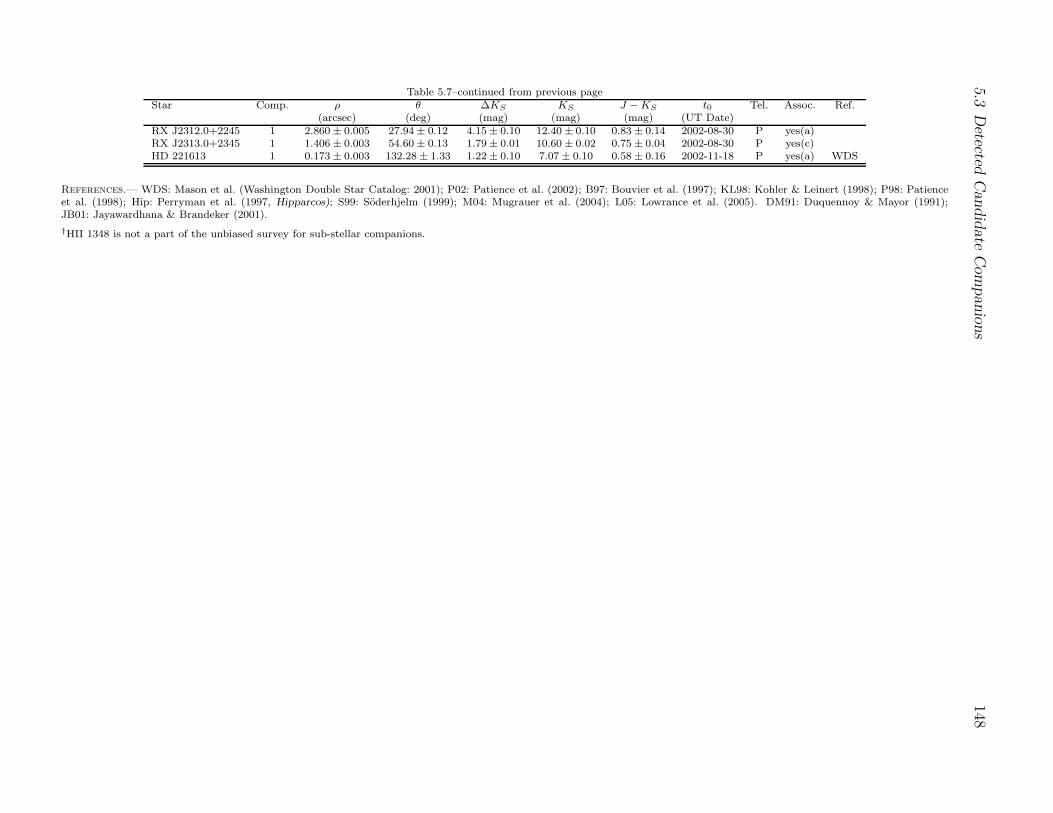
5.3D
etectedC
andid
ateC
ompan
ions
148Table 5.7–continued from previous page
Star Comp. ρ θ ∆KS KS J −KS t0 Tel. Assoc. Ref.(arcsec) (deg) (mag) (mag) (mag) (UT Date)
RX J2312.0+2245 1 2.860 ± 0.005 27.94 ± 0.12 4.15 ± 0.10 12.40 ± 0.10 0.83 ± 0.14 2002-08-30 P yes(a)RX J2313.0+2345 1 1.406 ± 0.003 54.60 ± 0.13 1.79 ± 0.01 10.60 ± 0.02 0.75 ± 0.04 2002-08-30 P yes(c)HD 221613 1 0.173 ± 0.003 132.28 ± 1.33 1.22 ± 0.10 7.07 ± 0.10 0.58 ± 0.16 2002-11-18 P yes(a) WDS
References.— WDS: Mason et al. (Washington Double Star Catalog: 2001); P02: Patience et al. (2002); B97: Bouvier et al. (1997); KL98: Kohler & Leinert (1998); P98: Patienceet al. (1998); Hip: Perryman et al. (1997, Hipparcos); S99: Soderhjelm (1999); M04: Mugrauer et al. (2004); L05: Lowrance et al. (2005). DM91: Duquennoy & Mayor (1991);JB01: Jayawardhana & Brandeker (2001).
†HII 1348 is not a part of the unbiased survey for sub-stellar companions.

5.3 Detected Candidate Companions 149
Table 5.8: Deep Sample Stars without Candidate Companions
HD 377 HD 691 HD 984HD 1405 HD 7661 HIP 6276HD 8907 HD 12039 HD 17925
1RXS J025751.8+115759 1RXS J030759.1+302032 1E 0307.4+14241E 0324.1-2012 HD 23208 HII 2147
1RXS J035028.0+163121 Pels 191 HD 285751RX J0442.5+0906 HD 35850 HD 38949
HD 43989 HD 70516 HD 72905HD 75393 HD 82558 HD 93528HD 95188 HD 101472 HD 107146SAO 2085 HD 132173 HD 139813
(PZ99) J160158.2-200811 HD 166181 HD 199019HD 209779 HD 217343
Table 5.9: Shallow Sample Stars without Candidate Companions
HD 6963 HD 8467 HD 8941 HD 11850HD 13382 HD 13507 HD 13974 HD 19019HD 19632 HE 699 HE 750 HE 767HE 848 HE 1234 HD 22879 HII 152HII 174 HII 173 HII 250 HII 314HII 514 HII 1015 HII 1200 HII 1776HII 2506 HII 2644 HII 2786 HII 3097HII 3179 HD 27466 vB 39 vB 63vB 64 vB 73 vB 79 vB 180vB 88 1RXS J043243.2–152003 vB 92 vB 93vB 183 vB 97 vB 99 vB 143HD 286264 HD 32850 HD 37216 HD 37006HD 38529 HD 64324 HD 66751 HD 72687HD 73668 HIP 42491 HD 75302 HD 76218HD 80606 HD 85301 HD 88638 HD 92788HD 98553 HD 100167 HD 101959 HD 102071HD 103432 HD 105631 HD 106156 HD 106252HD 121320 HD 122652 HD 133295 HD 136923HD 138004 HD 142229 RX J1600.6–2159 (PZ99) J160814.7–190833HD 145229 HD 150706 HD 153458 HD 154417HD 159222 HD 161897 HD 179949 HD 187897HD 190228 HD 193017 HD 195034 HD 199598HD 201219 HD 202108 HD 204277 HIP 106335HD 205905 HD 206374 HD 212291 HD 216275

5.3 Detected Candidate Companions 150
Figure 5.4: Magnitude difference ∆KS vs. angular separation ρ for all candidate companions dis-covered during the deep and shallow surveys. The various symbols denote: “•”—astrometricallyassociated companions; “×”—astrometrically unassociated background stars; and for objectswith insufficient astrometric data: “”—companions associated based on their JKS photom-etry; “+”—objects with JKS photometry inconsistent with association; “M”—undecided ob-jects. The encircled points show 3 brown-dwarf companions from the survey (encircled withsolid lines) and 1 companion at the stellar/sub-stellar boundary (HII 1348B; encircled with adotted line) that is not part of the unbiased survey for sub-stellar companions. Detection limitsfor the shallow (dashed line) and deep (solid and dotted lines) components of the survey are alsoshown. For the deep survey, the solid line shows the median contrast ∆KS, while the dottedlines delimit the 10–90 percentile region (cf. Fig. 5.3a). Binaries with separations smaller thanthe PALAO KS-band diffraction limit (0.09′′) were resolved only at J-band. Correspondingly,the plotted magnitude difference for these companions is the one at J .

5.4 Deciding Physical Association 151
5.4 Deciding Physical Association
The physical association of all candidate companions was decided following on one of the fol-lowing approaches: (1) common proper motion with the candidate primary, (2) a combinationof expected absolute KS magnitude (assuming equi-distance with the primary), near-IR col-ors, and background star density arguments, (3) extent of the radial profile of the candidatecompanion beyond that of a point-source PSF, or (4) use of prior-epoch astrometry from theexisting literature.
Criterion (1) is the argument of choice in companion studies, as it provides unambiguousevidence of association between two objects: whether as components of a gravitationally boundsystem or as members of a multi-star moving group sharing a common origin. The majority (150out of 183 or 82%) of associations and non-associations in this study are decided based on thisapproach (§5.4.1). Criterion (2) provides only a probabilistic estimate of physical associationand was applied only when astrometric follow-up was not obtained or the proper motion datawere inconclusive, and when additional J-band images were taken (§5.4.2). This criterionwas applied in 9 cases to exclude background interlopers and in 18 cases to establish physicalassociation of candidate stellar companions. Because of the larger scatter in near-IR colors forsub-stellar objects, this criterion was not useful for establishing physical association of candidatesub-stellar objects. Criterion (3) was used to weed out faint galaxies, which may otherwise havered near-IR colors, partially due to line-of-sight extinction in our own Galaxy, and thus poseas candidate sub-stellar objects for the preceding criterion. This criterion was applied in 3cases (§5.4.3). We resorted to the last approach (4) only for 3 candidate companions, for whichthe previous criteria could not be applied and for which astrometry existed from the literature(§5.4.4).
None of the above criteria were applicable to 105 candidate companions (36% of the total)that remained “undecided.” Most of these were faint and at large (> 5′′) angular separationsfrom their candidate host stars. Hence the vast majority are probably background stars (§5.4.5).
The association status of each candidate companion is indicated in the “Assoc.” column ofTables 5.6 and 5.7. “Yes(a)” and “no(a)” entries indicate bona fide astrometric companions anddissociated background stars, respectively. “Yes(c)” entries indicate stellar companions withphysical association constrained from their near-IR colors and projected absolute magnitude,while “no(c)” entries denote background objects identified through this criterion. “No(e)”entries denote extended sources, i.e., background galaxies. “Yes(p)” entries mark companionsfor which we have estimated association relying on prior-epoch astrometric measurements inthe existing literature. Finally, a “?” indicates candidate companions with inconclusive orunavailable astrometry and near-IR colors.
5.4.1 Proper Motion
We measured the angular separations and position angles of all candidate companions withrespect to their candidate primaries at all imaging epochs. The measurements were then usedin conjunction with the expected proper motion of the primaries to determine whether any ofthe candidate companions share their motion. The application and examples of the technique,using the preliminary astrometric calibration, were described in §3.3.3.2. Here we apply theimproved astrometric machinery of §4 to the entire sample.
Determining whether a field object shares the proper motion of the target star is based
5.4 Deciding Physical Association 152
on the combined application of two requirements: (i) that the change in the position of thecandidate companion relative to the primary is within 3σ of zero, and (ii) that the expectedchange in relative position of the candidate companion, had it been a stationary backgroundobject, is more than 3σ discrepant from the observed change. Often in cases of candidate close(.20 AU) binaries, criterion (i) was not satisfied, because of appreciable orbital motion insuch binaries. In such situations we have made sure (iii) that the observed change in relativeposition is much smaller (and less significant) than the expected change if the components ofthe candidate binary were not gravitationally bound.
When a relatively bright field star (4 < ∆KS . 8 mag), also visible in the shallow exposures,was present in the Palomar coronagraphic exposures, it was used as an additional astrometricreference. In cases where the subsequent astrometric measurements (with respect to the primaryand fainter field objects) showed such bright field stars to be approximately stationary, theycould be used to bootstrap the association of other candidate companions with the primary,circumventing the higher positional uncertainty arising from locating the primary behind thePHARO coronagraph (§4.6). This technique was particularly important in determining theassociation of systems in the distant USco (145 pc) and α Per (190 pc) regions, where theprimaries have small proper motions (.40mas yr−1), but where because of the low galacticlatitude (5 < |b| < 25) the images contain multiple background stars.
We monitored the change in relative position in terms of 4 measured quantities: change inright ascension (∆α), change in declination (∆δ), change in angular offset (∆ρ), and change inposition angle (∆θ). The statistical averages from multiple measurements of these quantitieswere monitored independently of one another, to minimize the need for covariant coordinatetransformations between (∆α,∆δ) and (∆ρ,∆θ). A 3σ change in any of the 4 quantities wasregarded as significant. For all but the faintest candidate companions, we obtained indepen-dent measurements for these quantities from the distortion-corrected detector pixel coordinatesin median-combined sub-sets (typically 4 per star) of the total number of exposures. For thefaintest objects visible only in the final median-combined image, we used the single measure-ment from that image and adopted errors corresponding to the empirical r.m.s. scatter of theastrometric calibration (§4.6), in addition to the object centering error.
In the following astrometric example we provide a step-by-step description of the applicationof criteria (i–iii) above, which was omitted in the published paper (§3.3.3.2). The example re-visits the two candidate companions to HD 49197, one of which was already identified as asub-stellar companion to the star.
5.4.1.1 Astrometric Example: The Candidate Companions to HD 49197 Re-visited
The first two epochs of imaging observations of HD 49197 were presented in Table 3.2 andFigure 3.5. An additional set of coronagraphic imaging observations was obtained at Palomaron 7 Feb, 2004. The astrometry was re-done using the updated pixel scale for PHARO (§4). Themore distant and brighter of the two candidate companions to HD 49197 (object 1 in Table 5.6)was seen both in the shallow non-coronagraphic and in the deep coronagraphic exposures of thestar and could thus be used as an additional astrometric reference to bootstrap the position ofthe primary behind the coronagraph with greater astrometric precision. (§4.6).
Table 5.10 lists the measured change in position (∆α, ∆δ, ∆ρ, and ∆θ), and the statisticalsignificance of the change (σ(∆α), σ(∆δ), etc.), for the candidate companions with respect
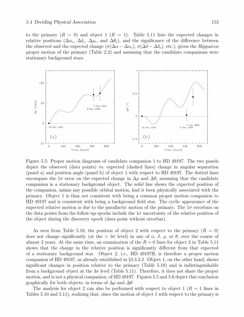
5.4 Deciding Physical Association 153
to the primary (R = 0) and object 1 (R = 1). Table 5.11 lists the expected changes inrelative positions (∆αe, ∆δe, ∆ρe, and ∆θe), and the significance of the difference betweenthe observed and the expected change (σ(∆α−∆αe), σ(∆δ −∆δe), etc.), given the Hipparcosproper motion of the primary (Table 2.2) and assuming that the candidate companions werestationary background stars.
Figure 5.5: Proper motion diagrams of candidate companion 1 to HD 49197. The two panelsdepict the observed (data points) vs. expected (dashed lines) change in angular separation(panel a) and position angle (panel b) of object 1 with respect to HD 49197. The dotted linesencompass the 1σ error on the expected change in ∆ρ and ∆θ, assuming that the candidatecompanion is a stationary background object. The solid line shows the expected position ofthe companion, minus any possible orbital motion, had it been physically associated with theprimary. Object 1 is thus not consistent with being a common proper motion companion toHD 49197 and is consistent with being a background field star. The cyclic appearance of theexpected relative motion is due to the parallactic motion of the primary. The 1σ errorbars onthe data points from the follow-up epochs include the 1σ uncertainty of the relative position ofthe object during the discovery epoch (data point without errorbar).
As seen from Table 5.10, the position of object 2 with respect to the primary (R = 0)does not change significantly (at the > 3σ level) in any of α, δ, ρ, or θ, over the course ofalmost 2 years. At the same time, an examination of the R = 0 lines for object 2 in Table 5.11shows that the change in the relative position is significantly different from that expectedof a stationary background star. Object 2, i.e., HD 49197B, is therefore a proper motioncompanion of HD 49197, as already established in §3.3.3.2. Object 1, on the other hand, showssignificant changes in position relative to the primary (Table 5.10) and is indistinguishablefrom a background object at the 3σ level (Table 5.11). Therefore, it does not share the propermotion, and is not a physical companion, of HD 49197. Figures 5.5 and 5.6 depict this conclusiongraphically for both objects, in terms of ∆ρ and ∆θ.
The analysis for object 2 can also be performed with respect to object 1 (R = 1 lines inTables 5.10 and 5.11), realizing that, since the motion of object 1 with respect to the primary is
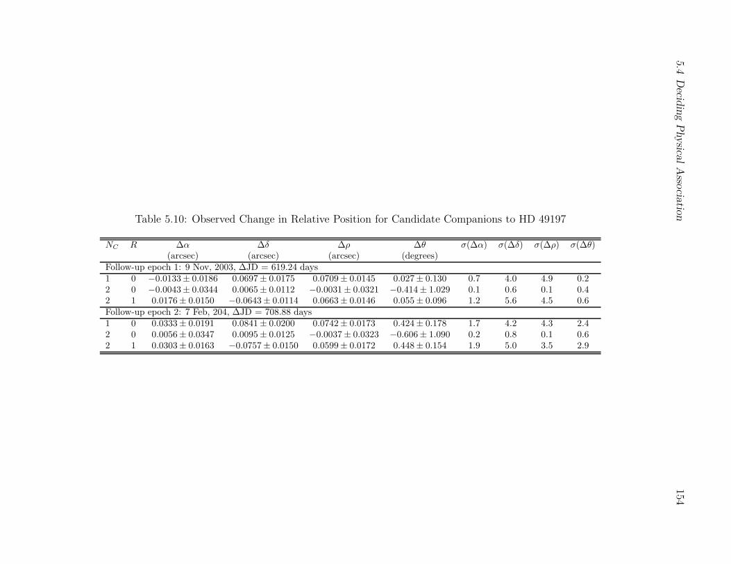
5.4D
ecidin
gP
hysical
Asso
ciation154
Table 5.10: Observed Change in Relative Position for Candidate Companions to HD 49197
NC R ∆α ∆δ ∆ρ ∆θ σ(∆α) σ(∆δ) σ(∆ρ) σ(∆θ)(arcsec) (arcsec) (arcsec) (degrees)
Follow-up epoch 1: 9 Nov, 2003, ∆JD = 619.24 days1 0 −0.0133± 0.0186 0.0697± 0.0175 0.0709± 0.0145 0.027± 0.130 0.7 4.0 4.9 0.22 0 −0.0043± 0.0344 0.0065± 0.0112 −0.0031± 0.0321 −0.414± 1.029 0.1 0.6 0.1 0.42 1 0.0176± 0.0150 −0.0643± 0.0114 0.0663± 0.0146 0.055± 0.096 1.2 5.6 4.5 0.6Follow-up epoch 2: 7 Feb, 204, ∆JD = 708.88 days1 0 0.0333± 0.0191 0.0841± 0.0200 0.0742± 0.0173 0.424± 0.178 1.7 4.2 4.3 2.42 0 0.0056± 0.0347 0.0095± 0.0125 −0.0037± 0.0323 −0.606± 1.090 0.2 0.8 0.1 0.62 1 0.0303± 0.0163 −0.0757± 0.0150 0.0599± 0.0172 0.448± 0.154 1.9 5.0 3.5 2.9

5.4D
ecidin
gP
hysical
Asso
ciation155
Table 5.11: Expected Change in Relative Position for Candidate Companions to HD 49197
NC R ∆αe ∆δe ∆ρe ∆θe σ(∆α − ∆αe) σ(∆δ − ∆δe) σ(∆ρ − ∆ρe) σ(∆θ − δθe)(arcsec) (arcsec) (arcsec) (degrees)
Follow-up epoch 1: 9 Nov, 2003, ∆JD = 619.24 days1 0 0.0316± 0.0021 0.0757± 0.0009 0.0664± 0.0013 0.3950± 0.017 2.4 0.3 0.3 2.82 0 0.0316± 0.0021 0.0757± 0.0009 0.0487± 0.0013 −3.8915± 0.128 1.0 6.2 1.6 3.42 1 0.0316± 0.0021 0.0757± 0.0009 −0.0590± 0.0013 −0.4656± 0.017 0.9 12.2 8.5 5.3Follow-up epoch 2: 7 Feb, 2004, ∆JD = 708.88 days1 0 0.0673± 0.0020 0.0913± 0.0010 0.0736± 0.0015 0.7070± 0.017 1.8 0.4 0.0 1.62 0 0.0673± 0.0020 0.0913± 0.0010 0.0873± 0.0015 −4.1847± 0.132 2.1 6.5 2.8 3.32 1 0.0673± 0.0020 0.0913± 0.0010 −0.0601± 0.0015 −0.7851± 0.016 5.9 11.1 7.0 8.0

5.4 Deciding Physical Association 156
Figure 5.6: Proper motion diagrams of candidate companion 2 to HD 49197. The panels, sym-bols, and lines are the same as in Figure 5.5. The motion of object 2 relative to HD 49197 is con-sistent with being 0 and is inconsistent with that of a background star. Object 2 (HD 49197B)is therefore a common proper motion companion to HD 49197 and, hence, physically associatedwith the star.
consistent with that of a stationary background star, the conclusions change: small values forσ(∆x) (where x is one of α, δ, ρ, or θ) and large values for σ(∆x−∆xe) indicate non-associationwith the primary, whereas large values for σ(∆x) and even larger values for σ(∆x − ∆xe)potentially indicate common proper motion with the primary. The astrometric measurementsfor object 2 with respect to object 1 thus re-affirm the association of object 1 with HD 49197.However, because field stars may have non-negligible proper motion, especially at the highlevel of astrometric precision of this survey, the assumption that any field object is stationaryneeds to be considered with care. Therefore, astrometric measurements relative to field objectscannot be used to establish the physical association of another candidate companion with theprimary, but need to be investigated in conjunction with the measurements with respect to theocculted star.
5.4.2 Absolute Magnitude, Near-IR Colors, and Background Object
Density
Systems with bright close-in candidate secondaries sometimes lack dual-epoch astrometry inthe survey. Such systems were given lower priority in follow-up observations, because theywere almost certainly bound, with stellar-mass secondaries. The astrometric analysis of §5.4.1is inapplicable in such cases. However, the candidate stellar secondaries in these systems arebright enough to be seen in the shallow non-coronagraphic exposures of each target, which inmost cases were obtained also in the J and H , in addition to the KS filter. Hence, for themajority of the candidate stellar systems lacking astrometric data, physical association can beestimated based on the near-IR colors and expected absolute magnitudes of the components.This approach can also be applied to fainter candidate companions, for which single-epoch J-

5.4 Deciding Physical Association 157
and KS-band coronagraphic data stars were taken at Keck.In evaluating the association of a candidate companion based on its near-IR photometry,
we looked for J −KS colors and apparent KS magnitude consistent with those of an object onthe same isochrone (usually, the main sequence) and at the same heliocentric distance as theprimary. For the sub-stellar regime, where the isochrones are not well-constrained, especiallynear the L/T transition (12 < MK < 14), we have relied on the empirical main sequence astraced by nearby M–T dwarfs with known parallaxes (Dahn et al., 2002; Leggett et al., 2002;Reid et al., 2004). All candidate companions with available J-band photometry, for which theastrometry was inconclusive, have had their physical association with the candidate primaryevaluated in this manner (Fig. 5.7). To limit the probability of misclassifying field stars ascompanions, positive associations have been adopted only for candidate companions within 5′′.
Figure 5.7: MKSvs. J −KS color-magnitude diagram for candidate companions in the sample
with obtained J-band photometry. The symbols are the same as in Figure 5.4. The additionalsmall dots denote M0–T8 dwarfs (MKS
& 4.5) with parallaxes from Leggett et al. (2002), Dahnet al. (2002), and Reid et al. (2004), and the F5–K5 sample stars (MKS
. 4.0 mag). The pointswith errorbars represent 3 confirmed brown-dwarf companions from the survey (solid errorbars)and 1 companion at stellar/sub-stellar boundary (HII 1348B; dotted errorbars) that does notbelong to the unbiased survey for sub-stellar companions (§6). The errorbars are representativeof the photometric precision of the survey, except for the large J−KS uncertainty of HD 49197B,which is unique. The vector in the upper right corresponds to 5 mag of V -band extinction,equivalent to a distance of ∼3 kpc, or a distance modulus of 12 mag in the galactic plane.

5.4 Deciding Physical Association 158
This approach was successful mostly for stellar-mass companions bluer than J −KS = 0.8(earlier than spectral type M0) because of the narrow width of their expected locus on thecolor-magnitude diagram. Therefore, projected companions in the background were apparentvia their discrepant absolute magnitudes. For early M dwarfs (M0–M6), the main sequence isnearly degenerate in J −KS over ∼4 mag in MKS
to within the errorbars and does not allowreliable association estimates. At even later spectral types, potentially representative of fainterbrown-dwarf companions, the higher photometric uncertainties and the larger empirical colorscatter at sub-stellar masses prevented the conclusive determination of physical association inall but a handful of faint projected companions. H-band photometry, where available, did notimprove the analysis because of the smaller spread in H −KS with respect to J −KS colors.
In addition to using near-IR colors, it is also possible to obtain a probabilistic estimate ofthe physical association for a candidate companion to its corresponding primary by comparingthe number of detected objects within the 12.5′′ survey radius to the surface density of starsat the relevant galactic coordinates down to the limiting magnitude of the survey. Because ofthe lack of large-area deep (KS . 20) near-IR survey data, we have constrained this type ofanalysis to only candidate companions in the shallow survey. Although the depth of the shallowsurvey varies depending on the use of the ND filter at Palomar, it is roughly comparable tothe completeness limit of the 2MASS survey: KS < 14.3 in unconfused regions of the sky.Therefore, for all candidate companions brighter than KS = 14.3, an empirical estimate of theassociation probability is possible from 2MASS. Given that the faintest primaries in the samplehave KS magnitudes of 9.6, such a probabilistic analysis can be performed on all candidatecompanions with ∆KS ≤ 4.7 mag.
To estimate the contamination fromKS ≤ 14.3 field stars, we counted the number of 2MASSobjects within a 5′-radius circular area offset by 12′ (to avoid bright artifacts) from each samplestar, and from that estimated the expected number of background objects in the 5′′-radius fieldof interest. We use this estimate as an equivalent of the purely geometrical chance alignmentprobability:
CAP = (number of 2MASS sources within 5′) × π(5′′)2
π(5 × 60′′)2. (5.1)
Table 5.12 lists the separations, ∆KS and KS magnitudes, and the CAPs for all sample starswith color companions (i.e., the ones with “yes(c)” entries in Tables 5.6 and 5.7). Most colorcompanions have chance alignment probabilities .2%, with the exception of HD 155902B andHE 935B, both of which are in very tight (< 0.1′′), and thus certainly physical, binaries. (Thesetwo systems are in fact below the resolution limits of the 95 mas PALAO KS-band PSF. Theirbinarity was only appreciated from PALAO J-band images, where the PSF is 50 mas wide.)The ensemble probability of at least one of the 17 color companions being a false positive is33%, or 16% after excluding HD 155902 and HE 935.
5.4.3 Source Extent
Only 3 of the detected sources have been flagged as extended, although a more careful objectprofile analysis will probably reveal a somewhat larger number, based on rough expectations ofthe surface density of background galaxies down to KS ≈ 20 mag. Determining source angularextent was not a primary objective of the survey, and source extent was judged only by eye.
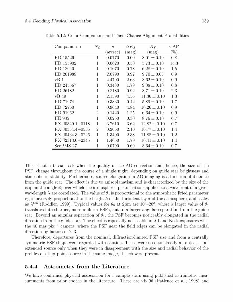
5.4 Deciding Physical Association 159
Table 5.12: Color Companions and Their Chance Alignment Probabilities
Companion to NC ρ ∆KS KS CAP(arcsec) (mag) (mag) (%)
HD 15526 1 0.0770 0.00 8.01 ± 0.10 0.8HD 155902 1 0.0620 0.50 5.73 ± 0.10 14.3HD 18940 1 0.1670 0.78 6.28 ± 0.10 1.5HD 201989 1 2.0790 3.97 9.70 ± 0.08 0.9vB 1 1 2.4700 2.63 8.62 ± 0.10 0.9HD 245567 1 0.3480 1.79 9.38 ± 0.10 0.8HD 26182 1 0.8180 0.92 8.71 ± 0.10 2.3vB 49 1 2.1390 4.56 11.36 ± 0.10 1.3HD 71974 1 0.3830 0.42 5.89 ± 0.10 1.7HD 72760 1 0.9640 4.84 10.26 ± 0.10 0.9HD 91962 2 0.1420 1.25 6.64 ± 0.10 0.9HE 935 1 0.0260 0.30 8.76 ± 0.10 6.7RX J0329.1+0118 1 3.7610 3.62 12.82 ± 0.10 0.7RX J0354.4+0535 2 0.2050 2.10 10.77 ± 0.10 1.4RX J0434.3+0226 1 1.3400 2.38 11.88 ± 0.10 1.2RX J2313.0+2345 1 1.4060 1.79 10.41 ± 0.10 1.4ScoPMS 27 1 0.0790 0.60 8.64 ± 0.10 0.7
This is not a trivial task when the quality of the AO correction and, hence, the size of thePSF, change throughout the course of a single night, depending on guide star brightness andatmospheric stability. Furthermore, source elongation in AO imaging is a function of distancefrom the guide star. The effect is due to anisoplanatism and is characterized by the size of theisoplanatic angle θ0 over which the atmospheric perturbations applied to a wavefront of a givenwavelength λ are correlated. The value of θ0 is proportional to the atmospheric Fried parameterr0, is inversely proportional to the height h of the turbulent layer of the atmosphere, and scalesas λ6/5 (Roddier, 1999). Typical values for θ0 at 2µm are 10′′–20′′, where a larger value of θ0translates into sharper, more uniform PSFs, out to a larger angular separation from the guidestar. Beyond an angular separation of θ0, the PSF becomes noticeably elongated in the radialdirection from the guide star. The effect is especially noticeable in J-band Keck exposures withthe 40 mas pix−1 camera, where the PSF near the field edges can be elongated in the radialdirection by factors of 2–3.
Therefore, departures from the nominal, diffraction-limited PSF size and from a centrallysymmetric PSF shape were regarded with caution. These were used to classify an object as anextended source only when they were in disagreement with the size and radial behavior of theprofiles of other point source in the same image, if such were present.
5.4.4 Astrometry from the Literature
We have confirmed physical association for 3 sample stars using published astrometric mea-surements from prior epochs in the literature. These are vB 96 (Patience et al., 1998) and
5.4 Deciding Physical Association 160
HD 150554 (Washington Double Star Catalog; Mason et al., 2001) in the shallow sample, andHD 165590 (Hipparcos; Perryman et al., 1997) in the deep sample.
5.4.5 Undecided Objects
A large fraction (36%) of the candidate companions remain astrometrically undecided at theend of the 3-year survey. The vast majority of these are faint objects in the fields of distant(>100 pc) stars with small apparent proper motions (<50 mas yr−1), often at low galacticlatitudes (b < 15), such as targets in α Per or in USco. Indeed, nearly all deep-sample starsbelonging to these two young associations have multiple companions at & 3′′ separations andwith ∆KS > 7 mag with undecided association status. These were often discovered onlyin follow-up deeper imaging with Keck and thus also lack the full time-span of observations.Judging by the large number of such candidate companions per star, and based on expectationsof the background star contamination rate at low galactic latitudes, likely all of these candidatecompanions are unassociated.
A smaller number of undecided companions reside around nearby (20–100 pc) stars at highergalactic latitudes, which were only added to the program in the last year of the survey: e.g.,the 20 stars in the extension of the FEPS sample (§2.3.2). Although second-epoch astrometryis not available for all candidate companions around these stars, they have been included inthe analysis because their higher proper motions ensured that quick (4–6 months) follow-upof any potential “interesting” companions would produce meaningful astrometric results. Suchwas indeed possible for candidate close-in faint companions to 4 of the newly-added stars(SAO 15880, HD 171488, HD 218738, and HD 218739).
Chapter 6
Survey Results and Analysis
Preliminary results from the survey for select stars were already presented in §3. These includedthe discovery of the first brown-dwarf companion from the survey, HD 49197B, and of threelow-mass stellar companions to HD 129333, V522 Per, and RX J0329.1+0118. In this chapterwe analyze the results from the complete survey, most notably the discovery of two additionalbona fide brown-dwarf companions, HD 203030B and ScoPMS 214B. In addition, we presentresults on a companion to HII 1348 at the stellar/sub-stellar limit, previously discovered byBouvier et al. (1997), but with unknown association status until now. Finally, 45 new stellarcompanions to stars in the sample are discussed.
6.1 Brown Dwarf Secondaries
All three of the bona fide sub-stellar companions were found in the deep survey. The remaininglow-mass companion, HII 1348B, was observed only because the existence of a faint candidatecompanion to HII 1348 was a priori known. The HII 1348A/B system is thus not part ofthe unbiased survey for sub-stellar companions. Here we address each of the four companionsindividually. Near-IR JHKS photometry for all is presented in Table 6.1. Their estimatedphysical properties are summarized in Table 6.2. Figure 6.1a compares the obtained MKS
absolute magnitudes and J −KS colors of the brown-dwarf companions with those predictedby the DUSTY (Chabrier et al., 2000) and COND (Baraffe et al., 2003) sub-stellar coolingmodels of the Lyon group. Figure 6.1b re-iterates the comparison in terms of the predictedluminosities and effective temperatures by the DUSTY models. (Burrows et al., 1997).
6.1.1 HD 49197B
The newly-discovered L-dwarf companion to HD 49197 was already discussed in §3.3. Theupdated astrometric analysis in §5.4.1.1 re-affirms the proper motion association of the sub-stellar companion with the primary. The adopted temperature and bolometric luminosity(Table 6.2) for the brown dwarf are based on the already determined spectral type (§3.3.3.3.1)and on spectral type vs. effective temperature and bolometric correction data for L and Tdwarfs from Vrba et al. (2004).
At a an age of ∼500 Myr and a spectral type of L4±1, HD 49197B is one of very few knownyoung ultra-cool (later than M7) brown dwarfs (§3.3.4.4). As such, it will be an importantreference point in future studies of the evolution of young sub-stellar objects.
161

6.1B
rown
Dw
arfSecon
daries
162
Table 6.1: Near-IR Photometry of the Confirmed and Candidate Brown Dwarfs
Object ∆KS J −H H −KS J −KS KS MKSMbol
(mag) (mag) (mag) (mag) (mag) (mag) (mag)HD 49197B 8.22 ± 0.11 1.2 ± 1.2 0.33 ± 0.20 1.6 ± 1.2 14.29 ± 0.14 11.04 ± 0.24 14.38 ± 0.24HD 203030B 9.58 ± 0.11 1.45 ± 0.22 0.47 ± 0.16 1.92 ± 0.22 16.23 ± 0.11 13.17 ± 0.15 16.1+0.3
−0.2
ScoPMS 214B 5.96 ± 0.09 0.67 ± 0.13 0.39 ± 0.13 1.06 ± 0.13 13.72 ± 0.09 7.91 ± 0.61 10.9 ± 0.6HII 1348B† 5.15 ± 0.09 0.74 ± 0.13 0.42 ± 0.13 1.16 ± 0.13 14.87 ± 0.09 9.25 ± 0.13 12.20 ± 0.16
† Not a member of the unbiased survey.

6.1B
rown
Dw
arfSecon
daries
163
Table 6.2: Estimated Physical Properties of the Sub-stellar Companions
Object Spectral Type† Teff Luminosity Age Mass Mass ratio Projected Separation(K) log(L/L) (Myr) (M) (AU)
HD 49197B L4±1 1800 ± 150 −3.86 ± 0.10 260–790 0.060+0.012−0.020 0.052 43
HD 203030B T0±1 1400 ± 50 −4.54+0.08−0.12 400 ± 200 0.035 ± 0.005 0.031 490
ScoPMS 214B M6±1 2700 ± 300 −2.46 ± 0.24 5 ± 1 0.025 ± 0.005 0.023 450HII 1348B‡ M6.5±1 2600 ± 300 −2.98 ± 0.06 125 ± 8 0.070 ± 0.005 0.093 145
† Except for that of HD 49197B, all other spectral types are estimated from near-IR photometry.‡ Not a member of the unbiased survey.

6.1 Brown Dwarf Secondaries 164
Figure 6.1: H–R diagrams of the new bona fide (circles) and candidate (triangle) brown dwarfs.(a) Near-IR color-magnitude diagram with the predictions of the Lyon group DUSTY andCOND models overlaid. Solid lines delineate 1, 10, 100, and 1000 Myr isochrones: from top tobottom in the DUSTY models, and from right to left in the COND models. Dotted lines showtracks of constant mass for 0.010 M and 0.030 M objects, whereas the dashed lines showthe hydrogen-burning limit (0.072 M) at solar metallicity. Mass also increases from top tobottom in the DUSTY models, and from right to left in the COND models. The small × pointsrepresent M–T dwarfs with known parallaxes Leggett et al. (2002); Reid et al. (2004); Gelinoet al. (2004). (b) L vs. Teff diagram, comparing the new brown dwarfs to predictions from theLyon group DUSTY models. The COND models are nearly identical to DUSTY in L − Teff
space. Symbols and line designations are the same as in panel (a). The degeneracy between sub-stellar age and mass is clearly identifiable from the nearly parallel sets of evolutionary tracksfor the two parameters. Note the much better agreement of the models with the estimatedparameters of HD 203030B in L vs. Teff space, compared to the inability of the models topredict the photometric properties (panel a) of this T0 dwarf.

6.1 Brown Dwarf Secondaries 165
6.1.2 HD 203030B
6.1.2.1 Astrometric Confirmation
The star HD 203030 was observed coronagraphically during three epochs at Palomar: 28 Aug,2002, 16 Jul, 2003, and 26 Jun, 2004. The time spans between the first and the subsequentepochs were ∆JD = 332.11 days and 668.17 days, respectively. The combined proper andparallactic motion of HD 203030 between the first and the final epoch amounted to 266 mas.A total of 8 candidate companions were identified in the deep image of the 25.6′′ × 25.6′′
PHARO field, 6 of which within the 12.5′′ survey radius (Fig. 6.2a). Such a high number offield objects was typical for the b = −16 galactic latitude of HD 203030. The brightest ofthe field objects (candidate companion 1 in Table 5.6) was also seen in the shallow exposuresof HD 203030 (Fig. 6.2b). The relative motion of this candidate companion with respect tothe primary was consistent with that of a stationary background star, as established from theshallow images. Thus, we used object 1 as an additional astrometric reference for all othercandidate companions to bootstrap the position of the primary behind the coronagraph withgreater astrometric precision (§4.6).
(b)
HD 203030; shallow
object 1
(a)
B
HD 203030; deep
object 1
Figure 6.2: Deep coronagraphic (a) and shallow non-coronagraphic (b) KS-band images ofHD 203030 from 28 Aug, 2002. The proper motion brown-dwarf companion HD 203030Bis indicated by an arrow in panel (a). The astrometry was done relative to the position ofbackground object 1, seen in both images. The broad 45-inclined jet-like feature in the deepimage is due to an oil streak across the secondary mirror of the Palomar 5 m telescope. Thesecondary was periodically cleaned subsequent to our identification of this feature, and the2003–2005 Palomar data lack this contamination. The images are 25.6′′ on a side; north is upand east is to the left.
We found that the third candidate companion to HD 203030 (Table 5.6) shared the apparentmotion of the primary, while its motion was discrepant from that of a stationary backgroundstar at the 7.1σ level in ∆ρ at the final imaging epoch. Therefore, object 3 is a proper motion
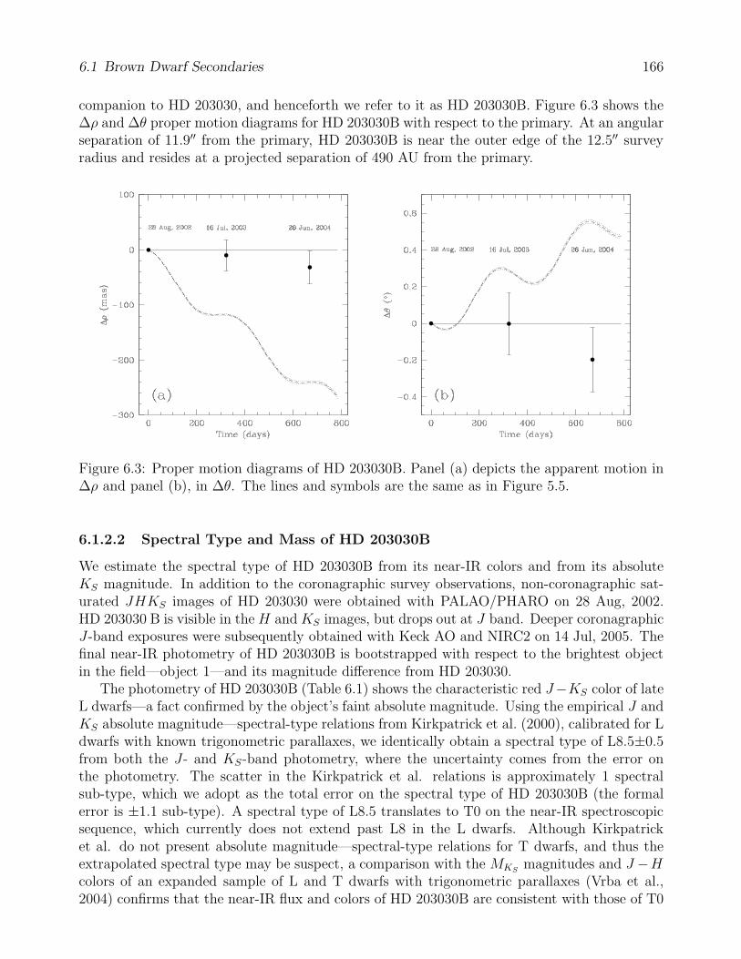
6.1 Brown Dwarf Secondaries 166
companion to HD 203030, and henceforth we refer to it as HD 203030B. Figure 6.3 shows the∆ρ and ∆θ proper motion diagrams for HD 203030B with respect to the primary. At an angularseparation of 11.9′′ from the primary, HD 203030B is near the outer edge of the 12.5′′ surveyradius and resides at a projected separation of 490 AU from the primary.
Figure 6.3: Proper motion diagrams of HD 203030B. Panel (a) depicts the apparent motion in∆ρ and panel (b), in ∆θ. The lines and symbols are the same as in Figure 5.5.
6.1.2.2 Spectral Type and Mass of HD 203030B
We estimate the spectral type of HD 203030B from its near-IR colors and from its absoluteKS magnitude. In addition to the coronagraphic survey observations, non-coronagraphic sat-urated JHKS images of HD 203030 were obtained with PALAO/PHARO on 28 Aug, 2002.HD 203030 B is visible in the H andKS images, but drops out at J band. Deeper coronagraphicJ-band exposures were subsequently obtained with Keck AO and NIRC2 on 14 Jul, 2005. Thefinal near-IR photometry of HD 203030B is bootstrapped with respect to the brightest objectin the field—object 1—and its magnitude difference from HD 203030.
The photometry of HD 203030B (Table 6.1) shows the characteristic red J−KS color of lateL dwarfs—a fact confirmed by the object’s faint absolute magnitude. Using the empirical J andKS absolute magnitude—spectral-type relations from Kirkpatrick et al. (2000), calibrated for Ldwarfs with known trigonometric parallaxes, we identically obtain a spectral type of L8.5±0.5from both the J- and KS-band photometry, where the uncertainty comes from the error onthe photometry. The scatter in the Kirkpatrick et al. relations is approximately 1 spectralsub-type, which we adopt as the total error on the spectral type of HD 203030B (the formalerror is ±1.1 sub-type). A spectral type of L8.5 translates to T0 on the near-IR spectroscopicsequence, which currently does not extend past L8 in the L dwarfs. Although Kirkpatricket al. do not present absolute magnitude—spectral-type relations for T dwarfs, and thus theextrapolated spectral type may be suspect, a comparison with the MKS
magnitudes and J −Hcolors of an expanded sample of L and T dwarfs with trigonometric parallaxes (Vrba et al.,2004) confirms that the near-IR flux and colors of HD 203030B are consistent with those of T0

6.1 Brown Dwarf Secondaries 167
dwarfs. We therefore adopt that as the spectral type for HD 203030B, with the ±1 sub-typeerror range translating to L7.5–T1. The corresponding effective temperature, nearly constantacross the L/T transition (e.g., Golimowski et al., 2004) is 1400 ± 50 K. Using a bolometriccorrection BCK = Mbol −MK = 2.9+0.3
−0.1 mag, where the Mbol and MK magnitudes for L7.5–T1dwarfs are taken from Table 9 of Vrba et al. (2004), we find a bolometric magnitude of Mbol =16.1+0.3
−0.2 mag, i.e., a luminosity of log(L/L) = −4.54+0.08−0.12 for HD 203030B, where we have
assumed Mbol = 4.74 mag for the Sun (Drilling & Landolt, 2000). HD 203030B is thus thecoolest, least luminous companion found around a young (<1 Gyr) star. Recently obtained K-band spectroscopy of this object is expected to open new insights on the elusive L/T transitionin ultra-cool dwarfs in evolutionary context.
We estimate the mass of HD 203030B using pre-main sequence tracks from the Lyon groups,assuming that the companion is co-eval with the primary. Given that the object is at the L/Ttransition, we obtain mass estimates by matching the near-IR flux of HD 203030B to predictionsfrom both the DUSTY (Chabrier et al., 2000) and COND (Baraffe et al., 2003) models. Wealso compare the estimated effective temperature and bolometric luminosity to predictions fromboth the Lyon and the Arizona (Burrows et al., 1997) groups.
The adopted age for HD 203030, based on its R′HK value, is 400 Myr (Table 2.2). Since
the R′HK index is only a secondary age indicator (see discussion in §2.2.2), we compare this
estimate to the ages inferred from other age indicators. Based on its galactic space motion,Montes et al. (2001b) list the star as a member of the IC 2391 supercluster, with an age of35–55 Myr. However, the relatively small Li I equivalent width of ≈ 60 ± 10 A seen in high-resolution optical spectra of HD 203030 (Strassmeier et al., 2000, White et al., in preparation)does not support such a young age at the late spectral type (G8) of the star. The observed Li I
absorption is less than the amount seen in 125 Myr old G8 Pleiades members and is comparableto the one seen in members of the 500 ± 100 Myr old Ursa Major moving group (King et al.,2003). Combining the R′
HK and lithium age estimates, we adopt an age of 400±200 Myr forHD 203030. The corresponding mass range for the MKS
magnitude of HD 203030B is ∼0.020–0.035 M from both the DUSTY and the COND models (Fig. 6.1). However, neither of themodels correctly predicts the J −KS color of HD 203030B. The DUSTY models over-predictit by ∼3 mag, while the COND models it by ∼1 mag (Fig. 6.1a). Therefore, we do not use thismass estimate. Instead, we adopt an estimate based on the inferred bolometric luminosity andeffective temperature of HD 203030B. These two indicators provide a more accurate renditionof the true thermodynamic state in brown-dwarf photospheres near the L/T transition (Baraffeet al., 2003), as is evident from a comparison of panels (a) and (b) in Figure 6.1. The estimatedmass is 0.030–0.040 M, identically confirmed from the models of Burrows et al. (1997). Thatis, HD 203030B is a brown dwarf.
The fact that HD 203030B is a brown dwarf could have been inferred, of course, withoutrelying on theoretical models, but just based on the late spectral type the object. Its estimatedeffective temperature of ∼1400 K, is far cooler than the minimum effective temperature attainedby main-sequence stars (∼2000 K, Fig. 1.2).

6.1 Brown Dwarf Secondaries 168
6.1.3 ScoPMS 214B
6.1.3.1 Astrometric Confirmation
ScoPMS 214 has a very small proper motion, only 22.8 mas yr−1 (bottom tenth percentile ofthe sample) and as a result required imaging at multiple epochs to discern whether any of the7 candidate companions within 12.5′′ shared the proper motion of the primary. The star wasobserved over 5 epochs between 2002 and 2005: on 30 Aug 2002 and 27 June 2004 at Palomar,and on 16 May 2003, 5 June 2004, and 13 Jul 2005 at Keck. The time spans between thefirst and the subsequent epochs were ∆JD=258.81, 645.37, 667.15, and 1048.19 days. Thecombined proper and parallactic motion of ScoPMS 214 between the first and the last epochwas 65.7 mas. This was sufficient to decide the physical association of the 3 closest and thebrightest of the remaining 4 candidate companions, but remained inadequate for the 3 faint(∆KS = 10.7 − 11.1) companions at angular separations > 10′′.
Most astrometric measurements for the star were calibrated with respect to the binaryWDS 18055+0230, except for the 16 May 2003 Keck data, which were calibrated from anobservation of WDS 15360+3948 taken on the following night. WDS 15360+3948 was not oneof the stars monitored at Palomar, and the astrometry calibrated with respect to it displays asignificant offset from the remaining observations. We ignore this data point in the followingdiscussion and consider only the remaining 4 epochs.
As in the cases of HD 49197 and HD 203030, one of the candidate companions in the field ofScoPMS 214, object 1 (later identified as ScoPMS 214B itself), was bright enough to be visiblewith sufficient signal-to-noise in the shallow non-coronagraphic Palomar images (Fig. 6.4). Thechanges in the relative positions of the remaining fainter candidate companions could thus bebootstrapped with respect to object 1. However, given that object 1 itself turned out to bethe proper motion companion to the primary, the context of the relative motions of the otherobjects with respect to it had to be accordingly re-considered.
The astrometric motion of object 1 relative to ScoPMS 214A is shown in Figure 6.5. Onlyat the final follow-up epoch is it possible to conclude that the apparent motion of object 1 isinconsistent with that of a background object. Even though the observed change δρ in angularseparation from the star is not inconsistent with that of a stationary background object, the lackof significant change in the position angle disagrees with that expected of a background objectat the 3.6σ level. On the other hand, the remaining 6 candidate companions all stay within1σ of their expected positions. Therefore, object 1 is a common proper motion companion ofScoPMS 214, and we will henceforth refer to it as ScoPMS 214B. At an angular separation of3.07′′ from the primary and a heliocentric distance of 145 pc, the projected separation betweenthe pair is 450 AU.
6.1.3.2 Spectral Type and Mass of ScoPMS 214B
ScoPMS 214B is visible in all shallow JHKS exposures of the primary. We therefore obtain theapparent magnitude of the companion by direct comparison with the 2MASS magnitudes ofScoPMS 214A. We find J −H = 0.67±0.13 mag, J −KS = 1.06±0.13 mag and, assuming thesame heliocentric distance as that of the primary, MKS
= 7.91 ± 0.61 mag. Using the “roughguide” to absolute near-IR magnitudes of K/M dwarfs (Reid et al., 2004), compiled from a20 pc volume limited survey of cool dwarfs from the NLTT proper motion catalog (Luyten,1980), we find that the spectral type of ScoPMS 214B is in the range M4–M6. The earlier
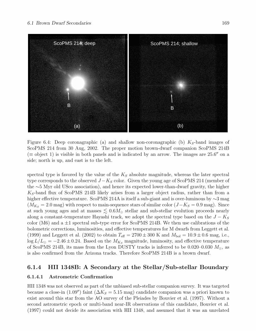
6.1 Brown Dwarf Secondaries 169
(b)
B
ScoPMS 214; shallow
(a)
B
ScoPMS 214; deep
Figure 6.4: Deep coronagraphic (a) and shallow non-coronagraphic (b) KS-band images ofScoPMS 214 from 30 Aug, 2002. The proper motion brown-dwarf companion ScoPMS 214B(≡ object 1) is visible in both panels and is indicated by an arrow. The images are 25.6′′ on aside; north is up, and east is to the left.
spectral type is favored by the value of the KS absolute magnitude, whereas the later spectraltype corresponds to the observed J−KS color. Given the young age of ScoPMS 214 (member ofthe ∼5 Myr old USco association), and hence its expected lower-than-dwarf gravity, the higherKS-band flux of ScoPMS 214B likely arises from a larger object radius, rather than from ahigher effective temperature. ScoPMS 214A is itself a sub-giant and is over-luminous by ∼3 mag(MKS
= 2.0 mag) with respect to main-sequence stars of similar color (J−KS = 0.9 mag). Sinceat such young ages and at masses . 0.6M stellar and sub-stellar evolution proceeds nearlyalong a constant-temperature Hayashi track, we adopt the spectral type based on the J −KS
color (M6) and a ±1 spectral sub-type error for ScoPMS 214B. We then use calibrations of thebolometric corrections, luminosities, and effective temperatures for M dwarfs from Leggett et al.(1999) and Leggett et al. (2002) to obtain Teff = 2700± 300 K and Mbol = 10.9± 0.6 mag, i.e.,logL/L = −2.46± 0.24. Based on the MKS
magnitude, luminosity, and effective temperatureof ScoPMS 214B, its mass from the Lyon DUSTY tracks is inferred to be 0.020–0.030 M, asis also confirmed from the Arizona tracks. Therefore ScoPMS 214B is a brown dwarf.
6.1.4 HII 1348B: A Secondary at the Stellar/Sub-stellar Boundary
6.1.4.1 Astrometric Confirmation
HII 1348 was not observed as part of the unbiased sub-stellar companion survey. It was targetedbecause a close-in (1.09′′) faint (∆KS = 5.15 mag) candidate companion was a priori known toexist around this star from the AO survey of the Pleiades by Bouvier et al. (1997). Without asecond astrometric epoch or multi-band near-IR observations of this candidate, Bouvier et al.(1997) could not decide its association with HII 1348, and assumed that it was an unrelated
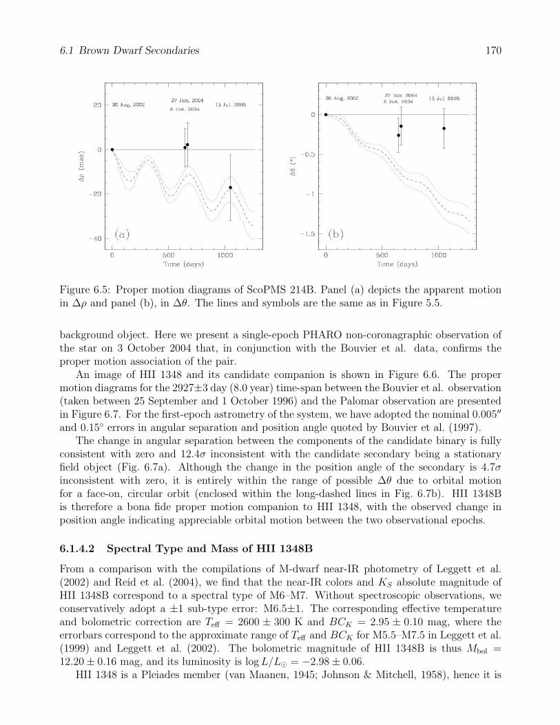
6.1 Brown Dwarf Secondaries 170
Figure 6.5: Proper motion diagrams of ScoPMS 214B. Panel (a) depicts the apparent motionin ∆ρ and panel (b), in ∆θ. The lines and symbols are the same as in Figure 5.5.
background object. Here we present a single-epoch PHARO non-coronagraphic observation ofthe star on 3 October 2004 that, in conjunction with the Bouvier et al. data, confirms theproper motion association of the pair.
An image of HII 1348 and its candidate companion is shown in Figure 6.6. The propermotion diagrams for the 2927±3 day (8.0 year) time-span between the Bouvier et al. observation(taken between 25 September and 1 October 1996) and the Palomar observation are presentedin Figure 6.7. For the first-epoch astrometry of the system, we have adopted the nominal 0.005′′
and 0.15 errors in angular separation and position angle quoted by Bouvier et al. (1997).The change in angular separation between the components of the candidate binary is fully
consistent with zero and 12.4σ inconsistent with the candidate secondary being a stationaryfield object (Fig. 6.7a). Although the change in the position angle of the secondary is 4.7σinconsistent with zero, it is entirely within the range of possible ∆θ due to orbital motionfor a face-on, circular orbit (enclosed within the long-dashed lines in Fig. 6.7b). HII 1348Bis therefore a bona fide proper motion companion to HII 1348, with the observed change inposition angle indicating appreciable orbital motion between the two observational epochs.
6.1.4.2 Spectral Type and Mass of HII 1348B
From a comparison with the compilations of M-dwarf near-IR photometry of Leggett et al.(2002) and Reid et al. (2004), we find that the near-IR colors and KS absolute magnitude ofHII 1348B correspond to a spectral type of M6–M7. Without spectroscopic observations, weconservatively adopt a ±1 sub-type error: M6.5±1. The corresponding effective temperatureand bolometric correction are Teff = 2600 ± 300 K and BCK = 2.95 ± 0.10 mag, where theerrorbars correspond to the approximate range of Teff and BCK for M5.5–M7.5 in Leggett et al.(1999) and Leggett et al. (2002). The bolometric magnitude of HII 1348B is thus Mbol =12.20 ± 0.16 mag, and its luminosity is logL/L = −2.98 ± 0.06.
HII 1348 is a Pleiades member (van Maanen, 1945; Johnson & Mitchell, 1958), hence it is
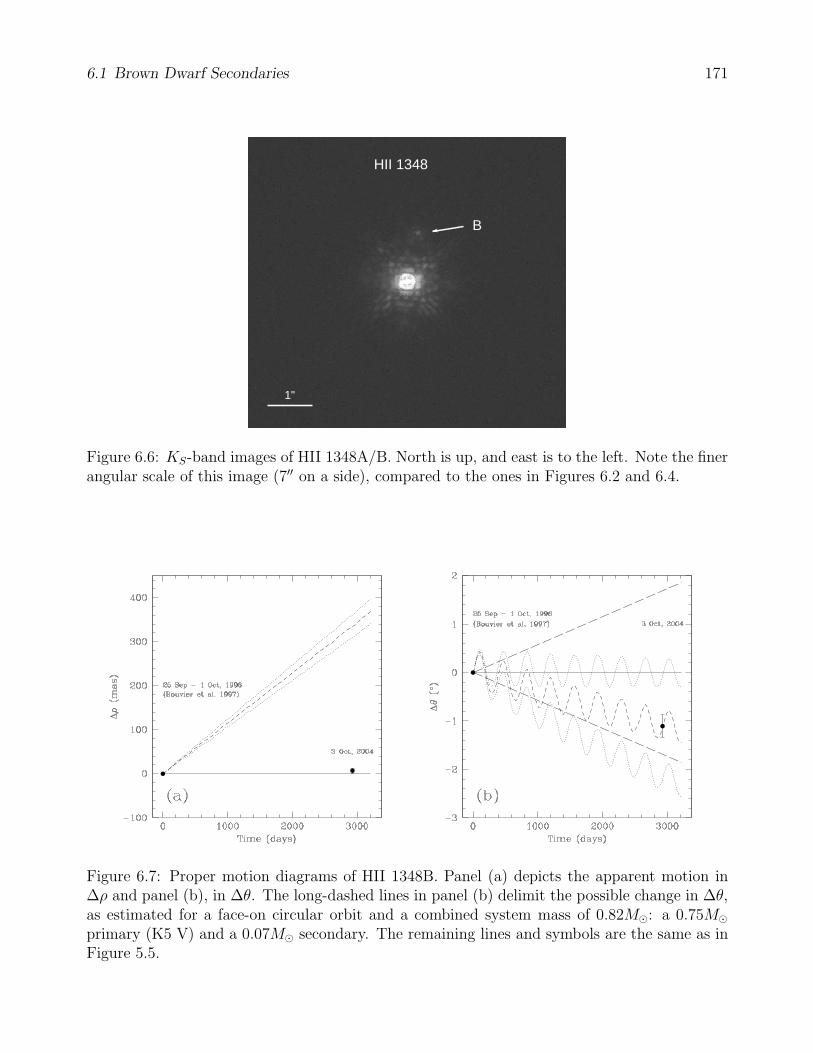
6.1 Brown Dwarf Secondaries 171
1"
B
HII 1348
Figure 6.6: KS-band images of HII 1348A/B. North is up, and east is to the left. Note the finerangular scale of this image (7′′ on a side), compared to the ones in Figures 6.2 and 6.4.
Figure 6.7: Proper motion diagrams of HII 1348B. Panel (a) depicts the apparent motion in∆ρ and panel (b), in ∆θ. The long-dashed lines in panel (b) delimit the possible change in ∆θ,as estimated for a face-on circular orbit and a combined system mass of 0.82M: a 0.75Mprimary (K5 V) and a 0.07M secondary. The remaining lines and symbols are the same as inFigure 5.5.

6.1 Brown Dwarf Secondaries 172
125±8 Myr old (Stauffer et al., 1998). For its absolute magnitude of MKS= 9.25 ± 0.13 mag,
the DUSTY models predict a mass of 0.070±0.005M. This mass range includes the hydrogen-burning mass limit, estimated at 0.072–0.075 M for solar metallicity (Chabrier et al., 2000;Burrows et al., 1997). It is therefore possible that the mass of HII 1348B lies above the hydrogen-burning limit and the object is, hence, a stellar companion. Because of the proximity of themass of HII 1348B to the hydrogen-burning limit and the relatively narrow mass error range, theissue of whether the object has sufficient mass to fuse hydrogen becomes of reduced importance,since present theory does not distinguish between the formation scenarios for low-mass stellarand brown-dwarf secondaries (Bate et al., 2003; Padoan & Nordlund, 2004).
6.1.5 A Critical Discussion of Sub-stellar Model Masses: Are theDetected Companions Truly Brown Dwarfs?
The mass estimates of brown dwarfs throughout this work are based on predictions by the-oretical models of sub-stellar evolution. The particular sets of models used are the DUSTYand COND cooling tracks from the Lyon group (Chabrier et al., 2000; Baraffe et al., 2003)and the cooling tracks from the Arizona group (Burrows et al., 1997). At <1 Gyr ages andfixed effective temperature and luminosity, the models from the two groups predict sub-stellarmasses that are consistent to within 15–20% of each other. However, both sets of models arestill very poorly constrained empirically, hence it is often unclear how well the predicted massescorrespond to reality. To answer the question posed here, we consider the current literature onempirical measurements of sub-stellar masses in its brief entirety. At each step, we compare theempirical checks to the masses predicted for the most closely corresponding new companions.
Dynamical masses in the sub-stellar regime exist only for two close binary brown dwarfs:Gl 569 Bab (Lane et al., 2001) and 2MASSW J0746425+2000321A/B (Bouy et al., 2004). Thecomponents in both systems are near the stellar/sub-stellar boundary and are inferred to be∼300 Myr old. These parameters are closest to the mass and age determined for HD 49197B(0.060M; 500 Myr) and could thus be used to test the model predictions for this object. Inthe case of 2MASSW J0746425+2000321A/B, the young age quoted by Bouy et al. (2004)is dependent on a comparison of the dynamical mass of the pair to theoretical models, andtherefore cannot be used as an independent test of the models. While this is also the case forthe age estimate adopted by Lane et al. (2001) for Gl 569Bab, the authors quote, in addition, anindependently-obtained age, as constrained from the observed rotation velocity, chromosphericand coronal activity, and space motion of the M2.5 primary Gl 569A. The agreement between theindependently-estimated (0.2–1.0 Gyr) and model-dependent (0.25–0.5 Gyr) ages for Gl 569 Babindicates that the theoretical models provide an adequate prediction of the physical parametersof the pair, and, by extrapolation, of HD 49197B. A further indication of the sub-stellar massof HD 49197B is that, at an age similar to that of Gl 569, HD 49197B has a later spectral type(L4±1; §3.3.3.3.1) than the 0.048–0.070 M M9 brown dwarf Gl 569Bb (Lane et al., 2001).
At masses just above the hydrogen-burning limit, the success of model predictions at youngages has recently been brought into question by Close et al. (2005), who compare model massesto their measurement of the dynamical mass of the newly-discovered component C in theAB Dor quadruple system. Close et al. find that, for an age of 50+50
−20 Myr for the AB Dorsystem (Zuckerman et al., 2004), both the Lyon and the Arizona group models underestimatethe 0.090±0.005M dynamical mass of AB Dor C by a factor of 1.3–2. That is, while both suitesof theoretical models predict sub-stellar masses for AB Dor C, the mass of the companion is

6.2 Incompleteness Analysis of the Deep Survey 173
decidedly stellar. However, this result has been more recently brought into question by Luhmanet al. (2005). By considering the location of all 4 components of the AB Dor system on an H-Rdiagram with respect to the loci of young open clusters with well-known ages, Luhman et al.find that the Zuckerman et al. (2004) age estimate is a factor of ∼2 in error. Luhman et al.find that AB Dor is of Pleiades age (100–125 Myr), which re-aligns the model mass predictionsfor AB Dor C with its dynamical mass. Therefore the mass estimate for HII 1348B, a Pleiadesmember at the sub-stellar/stellar boundary, may also be presumed safe, though its sub-stellarnature remains uncertain.
No dynamical masses have been measured for lower-mass, . 0.050M, brown dwarfs. Modelpredictions for low-mass sub-stellar objects remain less certain. Nevertheless, semi-empiricaltests of theoretical models at such masses exist (Mohanty et al., 2004). Mohanty et al. comparehigh-resolution spectra of young brown dwarfs in Upper Scorpius and Taurus to syntheticspectral templates, and use surface gravity-sensitive features in the spectra to calculate sub-stellar masses. While this approach does not rely on dynamical masses and hinges on theaccuracy of the model spectra, it is independent of the evolutionary aspect of the models.Given the known ages of objects in Upper Scorpius (5 ± 1 Myr; Preibisch et al., 2002) andTaurus (≈ 1 Myr; Myers et al., 1987), the Mohanty et al. analysis allows a test of the mass-agerelation in evolutionary models of sub-stellar objects. The authors find that the Lyon groupmodels provide a good approximation to ≥ 0.030M masses derived from fits to theoreticalspectral templates. This lower mass limit is similar to the masses of the remaining 2 browndwarfs, ScoPMS 214B and HD 203030B, though only the age of ScoPMS 214B is in the age rangeaddressed by Mohanty et al. (2004). The accuracy of the sub-stellar mass for ScoPMS 214B istherefore confirmed. However, the mass of HD 203030B remains less well-constrained.
Indeed, no currently existing empirical body of evidence can provide an independent checkon the mass estimate of HD 203030B. However, as already established in §6.1.2.2, the sub-stellarmass of the companion is beyond reasonable doubt.
6.2 Incompleteness Analysis of the Deep Survey
Having discovered three bona fide brown-dwarf companions among the 101 stars in the deepsample, we now estimate what fraction of the true sub-stellar companion population to Sun-likestars they represent. In this section, we address the factors affecting the survey completeness,state the analytical assumptions, and estimate a detection success rate of sub-stellar companionsas a function of the mass. We combine this estimate with the observational results to obtainthe underlying sub-stellar companion frequency.
6.2.1 Factors Affecting Incompleteness
Several factors need to be taken into account when estimating the detectability of sub-stellarcompanions around stars. These include: (i) possible sample bias against stars harboring sub-stellar secondaries, (ii) choice of sub-stellar cooling models, (iii) observational constraints (i.e.,imaging contrast and depth), and (iv) physical parameters of the stellar/sub-stellar system(flux ratio, age, heliocentric distance, orbit).
As already discussed in §2.4.2, the deep sample is, to a large extent, unbiased toward thepresence of sub-stellar companions, i.e., factor (i) can be ignored.
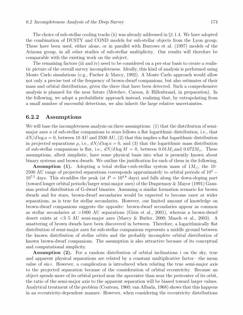
6.2 Incompleteness Analysis of the Deep Survey 174
The choice of sub-stellar cooling tracks (ii) was already addressed in §1.1.4. We have adoptedthe combination of DUSTY and COND models for sub-stellar objects from the Lyon group.These have been used, either alone, or in parallel with Burrows et al. (1997) models of theArizona group, in all other studies of sub-stellar multiplicity. Our results will therefore becomparable with the existing work on the subject.
The remaining factors (iii and iv) need to be considered on a per-star basis to create a realis-tic picture of the overall survey incompleteness. Ideally, this kind of analysis is performed usingMonte Carlo simulations (e.g., Fischer & Marcy, 1992). A Monte Carlo approach would allownot only a precise test of the frequency of brown-dwarf companions, but also estimates of theirmass and orbital distributions, given the three that have been detected. Such a comprehensiveanalysis is planned for the near future (Metchev, Carson, & Hillenbrand, in preparation). Inthe following, we adopt a probabilistic approach instead, realizing that, by extrapolating froma small number of successful detections, we also inherit the large relative uncertainties.
6.2.2 Assumptions
We will base the incompleteness analysis on three assumptions: (1) that the distribution of semi-major axes a of sub-stellar companions to stars follows a flat logarithmic distribution, i.e., thatdN/d log a = 0, between 10 AU and 2500 AU, (2) that this implies a flat logarithmic distributionin projected separations ρ, i.e., dN/d log a = 0, and (3) that the logarithmic mass distributionof sub-stellar companions is flat, i.e., dN/d logM = 0, between 0.01Mand 0.072M. Theseassumptions, albeit simplistic, have some physical basis into what is presently known aboutbinary systems and brown dwarfs. We outline the justification for each of them in the following.
Assumption (1). Adopting a total stellar+sub-stellar system mass of 1M, the 10–2500 AU range of projected separations corresponds approximately to orbital periods of 104 −107.5 days. This straddles the peak (at P = 104.8 days) and falls along the down-sloping part(toward longer orbital periods/larger semi-major axes) of the Duquennoy & Mayor (1991) Gaus-sian period distribution of G-dwarf binaries. Assuming a similar formation scenario for browndwarfs and for stars, brown-dwarf secondaries would be expected to become rarer at widerseparations, as is true for stellar secondaries. However, our limited amount of knowledge onbrown-dwarf companions suggests the opposite: brown-dwarf secondaries appear as commonas stellar secondaries at >1000 AU separations (Gizis et al., 2001), whereas a brown-dwarfdesert exists at <3–5 AU semi-major axes (Marcy & Butler, 2000; Mazeh et al., 2003). Asmattering of brown dwarfs have been discovered in between. Therefore, a logarithmically flatdistribution of semi-major axes for sub-stellar companions represents a middle ground betweenthe known distribution of stellar orbits and the probably incomplete orbital distribution ofknown brown-dwarf companions. The assumption is also attractive because of its conceptualand computational simplicity.
Assumption (2). For a random distribution of orbital inclinations i on the sky, trueand apparent physical separations are related by a constant multiplicative factor—the meanvalue of sin i. However, a complication is introduced when relating the true semi-major axisto the projected separation because of the consideration of orbital eccentricity. Because anobject spends more of its orbital period near the apocenter than near the pericenter of its orbit,the ratio of the semi-major axis to the apparent separation will be biased toward larger values.Analytical treatment of the problem (Couteau, 1960; van Albada, 1968) shows that this happensin an eccentricity-dependent manner. However, when considering the eccentricity distributions

6.2 Incompleteness Analysis of the Deep Survey 175
of observed binary populations (Kuiper, 1935a,b; Duquennoy & Mayor, 1991; Fischer & Marcy,1992), both analytical (van Albada, 1968) and empirical Monte Carlo (Fischer & Marcy, 1992)approaches yield the identical result: 〈log a〉 ≈ 〈log ρ〉+ 0.1. This indicates that the true semi-major axis and the measured projected separation are, on average, related by a multiplicativefactor of 1.26: 〈a〉 = 1.26〈ρ〉 and confirms the appropriateness of the current assumption.
Assumption (3). The evidence for a flat sub-stellar mass distribution stems from spectro-scopic estimates of the initial mass function (IMF) of isolated sub-stellar objects in star-formingregions (Briceno et al., 2002; Luhman et al., 2003a,b; Slesnick et al., 2004), which show a roughlyconstant number of sub-stellar objects per unit logM between 20 and 80MJup. While recentresults suggest (Mazeh et al., 2003) that the mass function of close (<4–5 AU) spectroscopicbinary stars differs from the IMF of isolated stars, there is as yet no such indication for widebinary star systems, the evolution of the individual components in which is likely to be in-fluenced less by the presence of the other. Furthermore, because of the limited number ofknown brown-dwarf companions to stars, the mass function of sub-stellar companions remainsunknown. Therefore, for lack of a better empirical alternative, we assume that the isolatedsub-stellar IMF is representative of the sub-stellar companion mass function, i.e., that the com-panion mass distribution is approximately logarithmically flat. In §6.2.3 we will show that aflat linear companion mass function, as may be assumed by an extrapolation of the Mazeh et al.(2003) data into the sub-stellar regime, will change the overall result negligibly. A decreasingmass function toward lower sub-stellar masses is also possible, though no supporting evidenceexists for that yet. Indeed, just based on the three 0.060 M, 0.035 M, and 0.025 M brown-dwarf companions discovered in the survey, the sub-stellar mass function of wide companionsseems to increase toward lower masses.
6.2.3 Incompleteness Analysis
Adopting the preceding assumptions, we now return to the discussion of the remaining factorsaffecting survey incompleteness: (iii) and (iv) from §6.2.1. We address the individual factorsin three incremental steps, as pertinent to: geometrical incompleteness, defined solely by theinner and outer working angles of the survey; observational incompleteness, defined by the fluxlimits of the survey; and orbital incompleteness, defined by the fraction of orbital phase spaceobserved. Throughout, we adopt the r.m.s. detection limits as determined for each star in§5.2 and assume that the primary ages and distances are fixed at their mean values listed inTable 2.2. The planned future Monte Carlo analysis will also address the uncertainties in theages and distances of the sample stars.
6.2.3.1 Geometrical Incompleteness
In deciding the range of projected separations that the study is most sensitive to, we look at thefull range of separations that have been explored between the inner and outer working anglesin the deep survey (§5.1). Figure 6.8 shows the fraction of sample stars (solid line) probingprojected separations between 3 AU and 3000 AU. It is immediately obvious, that only a verynarrow range of orbital separations, between 105 AU and 125 AU, is probed around 100% ofthe stars. All other orbital separations carry with them some degree of incompleteness, whichneeds to be taken into account. From a purely geometrical standpoint, i.e., ignoring imagingsensitivity, the limitations imposed by the inner (0.55′′) and outer (12.5′′) working angles of

6.2 Incompleteness Analysis of the Deep Survey 176
the survey amount to a factor of 1.96 incompleteness in log a between 6 AU and 2375 AU (theprojected separation range contained between the IWA for the nearest star and the OWA forthe farthest star). That is, provided that sub-stellar companions are detectable regardless oftheir brightness anywhere between 0.55′′ and 12.5′′ from each star, and provided that theirdistribution of semi-major axes a is logarithmically flat, only half of the companions residingin the 6–2375 AU projected separation range would be detected.
As is evident from Figure 6.8, such a wide range of orbital separations includes regionsprobed around only a small fraction of the stars. Consideration of the full 6–2375 AU rangewill thus induce poorly substantiated extrapolations of the companion frequency. Instead, wechoose to limit the analysis to projected separations explored around at least one-third (i.e., 34)of the stars in the deep sample. The corresponding narrower range, 22–1262 AU, is delimitedby the dashed lines in Figure 6.8. The region has a geometrical incompleteness factor of 1.40(cf. 1.96 for the full 6–2375 AU range above). That is, 1/1.40 = 71.4% of all companionswith projected separations between 22-1262 AU should be recovered by the survey, if they aresufficiently bright.
Figure 6.8: Projected physical separations probed in the deep sample survey. The verticaldashed lines delimit the region, 22–1262 AU, in which every apparent separation interval wasprobed around at least one third of the stars. The geometrical incompleteness factor is 1.40,i.e., 1/1.40 = 71.4% of all companions in this separation range should have been detected.

6.2 Incompleteness Analysis of the Deep Survey 177
6.2.3.2 Observational Incompleteness
Following an analogous approach to the one in the preceding discussion, we find the range ofcompanion masses that have been effectively probed between the established physical separationlimits of the deep survey. Because mass is not a direct observable, we use the absolute K-bandmagnitude of a sub-stellar object as a proxy for its mass, based on the Lyon suite of theoreticalmodels. We do not apply a conversion between the observed KS magnitudes and the CITK-band magnitudes calculated by the Lyon group. The difference is < 0.1 mag throughoutthe L-dwarf regime and increases to only KCIT −KS & 0.2 mag for >T5 dwarfs (Stephens &Leggett, 2004). The discrepancy between the K and KS magnitudes is thus likely to be smallerthan the accuracy of the theoretical predictions.
We test for discrete values of the sub-stellar mass and age: 0.005, 0.010, 0.012, 0.015, 0.020,0.030, 0.040, 0.050, 0.060, and 0.072 M, and 5, 10, 50, 100, and 500 Myr, respectively, aslisted in the DUSTY model tables of Chabrier et al. (2000). These mass and age ranges reflectthe range of possibly detectable sub-stellar masses and the age range of the stars in the deepsample. At the lowest sub-stellar masses, where at the older ages the models predict effectivetemperatures below 1400 K (the L/T dwarf transition temperature), we have used the CONDmodels, which are better suited to model the cloudless photospheres of T dwarfs. We haverounded intermediate stellar ages to the nearest (in logarithmic space) of the discrete agesabove. We then compare the companion fluxes for the range of sub-stellar masses to the fluxlimits for each star in the deep sample. In this manner, for each star in the sample, we obtaina range of projected separations over which a companion of a given mass would be visible.Summing over the stars in the entire sample, we estimate the observational incompleteness ofthe survey, i.e., with the actual flux limits taken into account.
The observational completeness at each discrete sub-stellar mass value is presented by thefilled circles in Figure 6.9a. The geometrical (i.e., maximum possible) completeness limit,estimated above at 71.4% for the 22–1262 AU range, is shown by the horizontal continuousline. The vertical dotted lines mark the mass limits of sustained deuterium (D) and hydrogen(H) burning (0.012M and 0.072M respectively). Figure 6.9a demonstrates that the deepsurvey is not flux limited above the H-burning mass limit, where the observational completenessreaches the geometrical limit. The Figure also shows that the observational completeness is>50% for all sub-stellar objects above the D-burning limit, though it drops rapidly below that.We therefore define 0.012–0.072M as the sub-stellar mass range, over which my survey achievessufficient sensitivity. This comprises the entire brown-dwarf mass range, that is, if a “browndwarf” is defined to be an object with mass lower than the H-burning limit and higher thanthe D-burning limit.
Adopting a uniform dN/d logM mass distribution for sub-stellar companions, we find thatthe survey is 65.3% complete to 0.012–0.072M sub-stellar companions at apparent separationsof 22–1252 AU from their host stars. The assumption of a uniform mass distribution per linearmass interval (dN/dM = 0) increases the observational completeness only slightly, to 68.4%.
What this means is that for every sub-stellar companion found at a projected separationbetween 22 AU and 1262 AU in the deep survey, another ≈1/3 companions within the samerange of projected separations were missed. Given that all 3 of the discovered sub-stellarsecondaries in the survey reside within this range, we expect that one more companion hasremained undiscovered. This companion could be a low-mass brown dwarf at a small angularseparation from one of the distant stars in the sample, where it was either occulted by the

6.2 Incompleteness Analysis of the Deep Survey 178
Figure 6.9: (a) Observational completeness without (circles) and with (triangles) the inclusionof single-visit obscurational completeness (SVOC; Brown, 2004) as a function of companionmass in the deep sample survey. The filled circles represent the fraction of companions of agiven mass that would be detectable within a projected separation of 22–1262 AU from allsample stars (§6.2.3.2). The triangles represent a similarly defined fraction, but for a 28–1590 AU range of semi-major axes (i.e., projected separation × 1.26; §6.2.3.3). Both sets offractions are calculated assuming a flat logarithmic distribution of orbital semi-major axes a.The horizontal lines delimit the maximum possible observational (continuous line) and orbital(long-dashed line) completeness at any given mass over these AU ranges. The vertical dottedlines mark the deuterium- (D) and hydrogen- (H) burning mass limits. (b) Same as Figure 6.8,but for the true semi-major axis and for a range of companion masses (dotted lines labeled withsub-stellar masses in MJup). The solid curve delineates the geometrical completeness and thelong-dashed curve, the SVOC (cf. panel a). The vertical short-dashed lines have been adjustedfrom their positions in Figure 6.8 to delimit the mean range of semi-major axes, 28–1590 AU,probed by the survey.

6.2 Incompleteness Analysis of the Deep Survey 179
coronagraph, or was lost in the glare of its host star. Alternatively, it could be a wide companionto one of the nearest stars, that was not considered or detected, because it fell outside the 12.5′′
OWA.
6.2.3.3 Orbital Incompleteness
The analysis so far has dealt only with the projected separation of sub-stellar companions.We now consider the full range of possible orbital inclinations and eccentricities, adopting themultiplicative factor of 1.26 in relating the projected separation ρ to the true semi-major axisa (§6.2.2). The range of orbital semi-major axes probed by the survey is therefore on averagea factor of 1.26 wider and further from the star: 28–1590 AU.
However, the adoption of the multiplicative correction does not exhaust the discussion oforbital incompleteness. Because companions on orbits with non-zero inclinations and eccen-tricities spend most of their time at projected separations ρ 6= a/1.26, they may still be missedin the survey. The most likely scenarios in which this can occur are for companions on highlyinclined and/or eccentric orbits. A sub-stellar companion on an inclined orbit may by missedbecause its projected separation from the star was too small (<22 AU) and fell in a regionwhere the imaging contrast was insufficient. Alternatively, an object on a highly eccentric orbitmay be missed because it spends most of its time near apocenter and could conceivably falloutside the survey OWA.
With a small number of successful sub-stellar companion detections, orbital incompletenessissues are best addressed through Monte Carlo simulations. Such have been performed for awide range of realistic orbital inclinations and eccentricities in a study by Brown (2004), theresults of which we adopt here.
Brown’s work investigates the detectability of populations of habitable extra-solar terrestrialplanets with a range of orbital distributions by the Terrestrial Planet Finder–Coronagraph(TPF–C). Although the angular scales and the levels of imaging contrast between the presentcoronagraphic survey and the design specifications for TPF–C are vastly different (TPF–C isexpected to have a factor of ≈2.5 smaller IWA and attain ∼ 106 higher contrast!), the problemis conceptually the same: determine the completeness to orbits with a certain semi-major axis,given a coronagraph of a fixed radius. Brown (2004) presents his results in terms of the ratio αof the semi-major axis to the obscuration radius, so they are universally scalable. His analysisdoes not include treatment of imaging contrast or limiting flux (these are addressed in a follow-up work: Brown, 2005), which makes it suitable to apply to results that have already beencorrected for these effects: as already done in §6.2.3.2.
Brown (2004) finds that the detectability of orbiting companions in a single-visit observationis a strong function of α between α = 1 and 2. What he terms the “single visit obscurationalcompleteness” (SVOC), varies between ≈30% at α = 1 and ≈85% at α = 1.9 (Fig. 6.10).Higher SVOC, at the 95% and 99% levels, is achieved only for α = 3.2 and 7.1, respectively.The result is largely independent (< 10%) of the assumed orbital eccentricity e for 0 ≤ e ≤ 0.35.
We adopt the results of Brown’s analysis and use the SVOC values for an eccentricity of 0.35(Table 4 in Brown, 2004)—a value near the peak of the eccentricity distribution of G-dwarfbinaries with > 103 day periods (Duquennoy & Mayor, 1991). We calculate the SVOC onthe image of each star in the sample, for each of the discrete candidate companion masses inthe 0.005–0.072 M range (§6.2.3.2). We define the minimum projected separation at whicha companion of a given mass is detectable as the effective obscuration radius for that mass.

6.2 Incompleteness Analysis of the Deep Survey 180
Figure 6.10: Orbital incompleteness (termed SVOC in Brown, 2004) of a single observation ata random epoch for companions having a particular size and shape of orbit. α is the ratio ofthe orbital semi-major axis of a hypothetical companion to the projected separation obscuredby a coronagraph. In the red area (SVOC=0), the apastron distance is smaller than theobscuration radius, and no companions are ever found. Contours in the gray area show values0 < SVOC < 1. The numbered points and the red X are irrelevant to the present discussion.(Brown, 2004)
6.2 Incompleteness Analysis of the Deep Survey 181
The results from the combined treatment of observational completeness (§6.2.3.2) and SVOCare shown in Figure 6.9a by filled triangles and in Figure 6.9b with the dotted lines. The long-dashed lines in Figures 6.9a,b delimit the maximum attainable SVOC, if companion brightnessis not a limiting factor. In panel (b), the SVOC limit coincides with the 75MJup (0.072M)line, indicating that the deep survey observations are maximally complete to objects at andabove the H-burning limit, i.e., to stars.
The additional consideration of the SVOC does not affect significantly the overall incom-pleteness of the survey. With the assumed companion mass and orbital semi-major axis dis-tribution, the overall completeness becomes 59.1%. This we adopt as the final estimate forthe survey. That is, given 3 detected companions with semi-major axes estimated in the 28–1590 AU range, two more companions with semi-major axes in the same range probably havebeen missed. The assumption of a linearly uniform mass distribution changes the completenessestimate only slightly, to 62.1%, i.e., not significantly affecting the overall completeness.
Finally, the consideration of the SVOC, as defined by Brown (2004), does not address allpossibilities for orbital incompleteness. As mentioned in the beginning of this discussion, acompanion on a highly-eccentric orbit may fall outside the OWA, even if its semi-major axiswas in the explored range. This additional factor, among possible other sources of orbital in-completeness, will be addressed in the forthcoming Monte Carlo analysis of the present data(Metchev et al., in preparation). However, judging by the small change (−6.2%) in the incom-pleteness correction induced by the consideration of the SVOC, it is unlikely that inclusion ofthe remaining factors affecting orbital incompleteness will decrease the overall survey detectionrate below 50%.
6.2.3.4 Further Incompleteness: Undecided Companion Candidates
Because the physical association status of a large fraction (37%) of candidate companionsdiscovered in the survey remains undecided (§5.4), it is possible that more bona fide sub-stellar companions may be confirmed in this data set in the future. This is not very likely,given that the vast majority of the undecided candidates are faint, reside in relatively high-density fields, and are at wide angular separations from their candidate primaries (Fig. 5.4),i.e., they have very high probabilities of being background stars. Nevertheless, the example ofHD 203030B—the faint, distant, sub-stellar companion to HD 203030, singled out from 5 othercandidate companions within 12.5′′ in the same image (given an average of 2 per star in thesample)—presents a strong indication that all projected companions need to be followed upastrometrically. A final round of observations to do so is in progress.
The confirmation of an additional brown-dwarf companion would increase the total numberto 4 and would imply that we have underestimated the success rate of the survey by a factor of1.25. That is, the survey could conceivably be 45% complete, and hence, the 59% completenessestimate from §6.2.3.3 is an upper limit. Taking into account other possible sources of incom-pleteness that have been ignored, such as the small selection bias against massive sub-stellarcompanions to K0–K5 dwarfs (§2.4.2), and the partial consideration of orbital incompleteness(§6.2.3.3), the overall detection rate may be even lower. However, given the small anticipatedmagnitudes of each of these two remaining effects, we expect that the overall completeness isnot less than 40%.
A lower estimate for the survey completeness will drive the expected rate of brown-dwarfcompanions higher. Because of the presently unquantified and likely unimportant nature of

6.3 Frequency of Wide Sub-stellar Companions to Young Solar Analogs 182
the additional sources of incompleteness, and for the sake of preserving statistical rigor, we willassume that the derived value of 59% provides an accurate estimate of the survey completeness.
6.3 Frequency of Wide Sub-stellar Companions to Young
Solar Analogs
We have now described the survey sample, the successful brown-dwarf companion detections,and the incompleteness of the survey. Based on 3 detections around 101 stars, and an estimated≈60% detection rate, we find that an ideal survey of the same size as ours will most likelydetect 0.012–0.072 M companions with 28–1590 AU (or, approximately, 30–1600 AU) semi-major axes around 5% of the stars in the sample. In order to determine the agreement of thisestimate with previous ones reported in the literature, we need to determine confidence limits.In addition, as we shall demonstrate shortly, while 3% (or 5%, for an ideal survey) may be themost likely detection rate, it is not the expectation (mean) frequency of substellar companions.
Throughout the remainder of this work, we will use the terms “sub-stellar companion” and“brown dwarf companion” to refer to a brown-dwarf secondary to a young Sun-like star, withmass and orbital semi-major axis as defined in the preceding paragraph.
First, we address the statistical uncertainty arising from the small number of successfuldetections: only 3 in 101 trials. The large number of experiments and the small number ofsuccessful outcomes mean that the probability of detecting x brown dwarfs given an expectednumber µ is governed by a Poisson probability distribution:
P (x|µ) =µxe−µ
x!. (6.1)
We are interested in finding what is the probability distribution for µ given x detections, i.e.,we need P (µ|x).
This is a standard problem in Bayesian statistical analysis (Bayes, 1763; Rainwater & Wu,1947). The result follows from Bayes’ Theorem (Rainwater & Wu, 1947; Papoulis, 1984):
P (µ|x) =P (x|µ)P (µ)
P (x), (6.2)
where the P ’s denote “probability distribution” rather than identical functional forms. P (µ) iscalled the “prior” and summarizes our expectation of the state of nature prior to the observa-tions. P (x|µ) is the “likelihood” that x outcomes are observed given a mean of µ, and P (µ|x)is the “posterior” probability that the state of nature is µ, given x positive outcomes. P (x) is anormalization factor, which ensures that the sum of all probable outcomes P (x|µ′), given someprobability P (µ′), is unity:
P (x) =
∫ ∞
0
P (x|µ′)P (µ′)dµ′. (6.3)
The physical (or philosophical, if you will) interpretation of Bayes’ Theorem can be summarizedin the following:
P (state of nature | evidence) =P (evidence | state of nature)P (state of nature)
normalizing factor. (6.4)

6.3 Frequency of Wide Sub-stellar Companions to Young Solar Analogs 183
Equation 6.3 is defined for the continuous, rather than discrete (in which the integral wouldbe replaced by a sum), formulation of Bayes’ Theorem. The P ’s are therefore, technically, notprobabilities, but probability density functions (p.d.f.). Given that the formation of a brown-dwarf companion is a process that may occur around any Sun-like star, not just the 101 inthe present sample, the use of the continuous limit is a valid approach because in principle thesurvey could be performed on an arbitrarily large sample.
As is standard practice in Bayesian analysis, we will assume that we have no a prioriknowledge of the state of nature, i.e., we choose a uniform flat prior: P (µ) = 1. In the contextof the survey, this means that we have assumed that all sub-stellar companion frequencies0 ≤ µ ≤ 1 are equally probable. Indeed, this is not a completely inadequate representation ofour current state of knowledge on the subject. We also performed tests with different uniformpriors that place more weight on smaller expected companion frequencies: P (µ) = log µ andP (µ) = 1/µ (µ > 0 in both cases). It may be argued that such priors better approximatethe expectation that the sub-stellar companion frequency is small. The effect of these was toincrease, rather than decrease, the estimated mean brown-dwarf companion frequency.
Inserting Equation 6.1 into Equations 6.2 and 6.3, we obtain
P (µ|x) = P (x|µ) =µxe−µ
x!. (6.5)
This result makes intuitive sense: the p.d.f. for µ is a distribution, that peaks at the observedsuccess rate x. That is, by assumption, x is the most likely observational outcome. We nowfind that the mean number of sub-stellar companion detections per survey, if the survey wereto be repeated multiple times on different samples of stars, is
〈µ〉 =
∫∞0µµ
xe−µ
x!dµ
∫∞0
µxe−µ
x!
= 4. (6.6)
This may at first seem surprising, given that the number of successful experiment outcomes was3, rather than 4, out of a total of 101. The appearance of this “extra” sub-stellar companion isdue neither to the incompleteness of the survey (§6.2.3.1–6.2.3.3) nor to the possible existence ofmore bona fide companions among the undecided ones (§6.2.3.4). Rather, the difference betweenthe maximum-likelihood and the expectation (mean) value is a property of the continuousPoisson distribution (Fig. 6.11) due to its asymmetry around the mean.
To obtain the nσ upper and lower (µ+nσ and µ−nσ) confidence intervals for 〈µ〉, we set thedefinite integral of P (µ|x) between µ+nσ and µ−nσ to the corresponding nσ significance level:
∫ unσ
0
µxe−µ
x!=
0.841 n = 10.977 n = 20.9987 n = 3
(6.7)
∫ lnσ
0
µxe−µ
x!=
0.159 n = 10.023 n = 2.0.0013 n = 3
(6.8)
The resulting 1, 2, and 3σ (68.2%, 95.4%, and 99.7%) confidence limits are 2.1–5.9, 1.1–8.9,and 0.5–12.7 detectable companions on average for a survey of 101 stars.
Having addressed the statistical uncertainties associated with the small number of compan-

6.4 Stellar Secondaries 184
Figure 6.11: Probability density distribution P (µ|x = 3) for the sub-stellar companion fre-quency per 101 stars, given x = 3 detections. The curve is a continuous Poisson distribution(Eqn. 6.5), with a maximum likelihood value of µML = 3 (equal to the number of detections x),but a mean value of 〈µ〉 = x+ 1 = 4. The 68% (1σ) confidence interval on 〈µ〉 is indicated bythe horizontal errorbar above the curve.
ion detections, we now apply the estimated survey completeness correction (59%) to the meanvalue and to the confidence interval limits of µ. We thus find that 6.8+3.2
−3.2% (1σ limits; +8.3−4.9: 2σ
limits; +14.7−5.9 : 3σ limits) of F5–K5 stars in the 3–500 Myr age range have sub-stellar companions
with semi-major axes between 30 AU and 1600 AU.
6.4 Stellar Secondaries
The entire survey produced 45 new stellar companions to 44 stars. Physical association of afurther 31 known and suspected binary stars was confirmed (§6.4.3). One star, HD 91962,a priori considered single, was resolved into a triple system. No higher-order multiples wereresolved. However, some of the newly-resolved binary systems are themselves known to becomponents of higher-order visual and/or spectroscopic binaries. The statistics and multiplicityof these systems will be the subject of a future study.
The majority (57 out of 75) of the binaries and the triple system were members of theshallow survey, as a result of the requirement that no ∆KS < 4.0 candidate companions werepresent around stars in the deep survey (§2.3.2). The binaries found in the deep survey eitherhave low mass ratios, such that the secondary is more than 4 mag fainter than the primaryat KS, or have < 0.8′′ angular separations, so that the PSFs of both components could be fitunder the 1′′ coronagraph.
KS-band magnitudes and J − KS colors of the stellar companions were already includedin Tables 5.6 and 5.7. From these we infer KS-band absolute magnitudes for the companions,using the known distance to the primary (Table 2.2), and masses, using the stellar evolutionary

6.4 Stellar Secondaries 185
models of Baraffe et al. (1998). Table 6.3 lists these two quantities for each bona fide stellarcompanion, along with projected separations and system mass ratios.
Table 6.3: Properties of the Detected Stellar Companions
Companion MKSProjected Separation M2 q
(mag) (AU) (M)HD 224873B 4.12 ± 0.24 62.1 0.99 0.98HD 9472B 9.24 ± 0.11 92.2 0.10 0.10RE J0137+18B 2.74 ± 0.29 108.2 1.06 1.00HD 13531B 7.81 ± 0.12 18.6 0.19 0.20HD 15526B 3.79 ± 0.54 8.2 0.90 0.791RXS J025223.5+372914B 4.62 ± 1.09 108.3 0.70 0.612RE J0255+474B 3.82 ± 1.09 106.5 0.91 1.00RX J0258.4+2947B 5.15 ± 1.09 8.6 0.58 0.67HD 18940B 3.28 ± 0.11 5.7 0.84 0.73vB 1B 5.45 ± 0.10 106.5 0.56 0.47HE 373B 8.20 ± 0.16 395.4 0.11 0.09HE 696B 5.91 ± 0.16 85.1 0.44 0.43RX J0329.1+0118B 7.82 ± 1.09 376.1 0.11 0.12HE 935B 2.98 ± 0.16 4.9 1.15 0.86HII 102B 6.10 ± 0.14 478.7 0.43 0.39HII 120B 8.91 ± 0.18 1414.2 0.09 0.081RXS J034423.3+281224B 3.62 ± 1.09 42.5 0.96 0.74HII 571B 7.70 ± 0.14 519.1 0.17 0.17HII 1182B 7.85 ± 0.13 148.0 0.13 0.12HII 2106B 5.95 ± 0.14 31.9 0.46 0.50RX J0348.9+0110B 4.52 ± 1.09 4.7 0.85 0.81HII 2278B 3.96 ± 0.14 44.0 0.87 0.79HII 2881B 4.47 ± 0.13 13.2 0.81 0.87RX J0354.4+0535B 5.92 ± 1.09 20.5 0.48 0.48HD 285281B 3.41 ± 1.09 107.8 0.87 0.46HD 284135B 2.90 ± 1.09 51.4 0.94 0.72HD 281691B 4.20 ± 1.09 947.5 0.75 0.66HD 26182B 4.09 ± 1.09 81.8 0.79 0.66HD 284266B 6.16 ± 1.09 79.7 0.43 0.39HD 26990B 4.09 ± 0.16 4.3 0.83 0.77vB 49B 7.60 ± 0.15 123.0 0.22 0.19vB 52B 5.84 ± 0.11 50.0 0.51 0.45vB 176B 4.26 ± 0.11 10.9 0.79 0.83vB 91B 4.84 ± 0.10 6.1 0.66 0.70vB 96B 4.33 ± 0.11 7.8 0.77 0.76continued on next page

6.4 Stellar Secondaries 186
Table 6.3 – continued from previous pageCompanion MKS
Projected Separation M2 q(mag) (AU) (M)
RX J0434.3+0226B 5.78 ± 0.35 215.7 0.40 0.45HD 282346B 4.45 ± 0.44 32.7 0.70 0.67HD 31950B 7.51 ± 1.09 259.6 0.13 0.121RXS J051111.1+281353B 3.51 ± 0.33 98.5 1.39 0.62HD 36869B 5.66 ± 0.64 592.6 0.36 0.30HD 245567B 3.85 ± 0.40 41.4 0.30 0.24HD 69076B 7.61 ± 0.26 41.9 0.24 0.26HD 71974B 4.14 ± 0.12 11.1 0.81 0.78HD 72760B 8.59 ± 0.11 21.0 0.13 0.15HD 77407B 6.70 ± 0.12 49.8 0.54 0.49HD 91782B 8.16 ± 0.15 56.1 0.23 0.20HD 91962B 4.19 ± 0.15 31.2 0.81 0.67HD 91962C 7.60 ± 0.16 5.2 0.83 0.69HD 92855B 7.91 ± 0.12 105.6 0.16 0.14HD 99565B 3.83 ± 0.21 14.3 0.88 0.82BPM 87617B 5.09 ± 1.09 12.4 0.61 0.83HD 108799B 4.31 ± 0.13 51.8 0.78 0.67HD 108944B 8.62 ± 0.18 85.4 0.41 0.34HD 112196B 9.13 ± 0.16 51.0 0.61 0.53HD 115043B 8.13 ± 0.11 42.6 0.17 0.15HD 129333B 5.93 ± 0.12 24.4 0.38 0.36HD 134319B 6.77 ± 0.10 235.7 0.22 0.22HD 135363B 5.04 ± 0.12 7.3 0.60 0.72HD 139498B 2.74 ± 0.20 39.5 1.22 0.75HD 142361B 4.14 ± 0.32 71.2 0.37 0.29ScoPMS 27B 3.33 ± 0.61 11.5 0.64 0.61ScoPMS 52B 2.34 ± 0.61 20.9 0.56 0.28(PZ99) J161329.3–231106B 5.47 ± 0.61 207.3 0.15 0.12(PZ99) J161411.0–230536B 2.56 ± 0.61 32.2 1.20 0.60HD 150554B 6.10 ± 0.14 521.8 0.45 0.39HD 152555B 6.73 ± 0.17 183.3 0.32 0.28HD 155902B 4.02 ± 0.13 1.7 0.84 0.77HD 157664B 2.89 ± 0.16 3.0 1.06 0.74HD 165590B 2.73 ± 0.15 16.8 1.24 1.00HD 199143B 4.75 ± 0.13 50.5 0.50 0.41HD 200746B 8.82 ± 0.34 10.0 0.62 0.57HD 201989B 7.31 ± 0.11 62.4 0.25 0.24RX J2312.0+2245B 6.52 ± 1.09 429.0 0.38 0.31RX J2313.0+2345B 4.72 ± 1.09 210.9 0.40 0.40HD 221613B 4.32 ± 0.11 5.7 0.72 0.65
A comprehensive study of the incompleteness of the stellar component of the companionsurvey is deferred to a later time. The main goal of the present work was to determine the

6.4 Stellar Secondaries 187
frequency of sub-stellar companions. Nevertheless, we briefly summarize the results on theobserved frequency of stellar multiples and their distribution of mass ratios below. We alsoaddress the possibility for dynamical mass determination in the systems found from previousimaging campaigns, for about half of which the present data reveal significant orbital motion.
6.4.1 Frequency of Multiple Systems
It is perhaps surprising that such a large fraction of stellar multiples was discovered in thesurvey despite a series of requirements aimed at excluding known binary stars from the sam-ple (§2.3). Seventy-two out of the 266 solar-type stars in the survey, or 27%, have q > 0.1stellar companions in the probed angular separation range. We compare this to the most com-prehensive study of multiplicity of solar analogs in the field to date: the combined study ofspectroscopic and visual binaries by Duquennoy & Mayor (1991).
At first glance, the observed binarity frequency is a factor of ≈2 lower (though not inconsis-tent, given the bias against binaries) than the Duquennoy & Mayor (1991) estimate that 57%of G-dwarf primaries have q > 0.1 secondaries. However, the AO survey covers only a limitedrange of orbital separations, whereas the Duquennoy & Mayor study covers both spectroscopicand visual G-dwarf binaries, with orbital periods between < 1 and 1010 days. Given the rangeof stellar heliocentric distances in the sample, 10–200 pc, and the angular limits of the survey,0.1′′−12.5′′, a least conservative estimate, without performing an analysis analogous to the onefor sub-stellar masses (§6.2.3), puts the probed separation range at 1–2500 AU. For a binarysystem with a combined mass in the 1–2M interval, the corresponding range of orbital periodsis 102.4–105.0 days. In reality, the survey may be up to 50% incomplete in this range of orbitalperiods or, equivalently, semi-major axes because of the inability to resolve close binaries atlarger heliocentric distances and because of the omission of wide companions to nearby starsdue to the limited detector field of view. Therefore, a completeness-corrected estimate of thebinarity of the sample stars over 102.4–105.0-day orbital periods will likely reside in the 40–50%range. Unfortunately, the complicated nature of the bias against binaries makes it difficult toobtain a more precise incompleteness correction.
Duquennoy & Mayor (1991) find that 22% of G dwarfs have q > 0.1 stellar companionswith 102.4–105.0-day periods, as estimated from their to the incompleteness-corrected perioddistribution. This is already lower than the observed fraction of 27% in the AO observationsand likely significantly different from the probable 40–50% incompleteness-corrected estimate.
The most likely explanation for this discrepancy is evolution of the stellar multiplicityfraction—a phenomenon that has been inferred from multiplicity studies of young star-formingregions, intermediate-aged open clusters, and old field stars. It is well-established (Ghez et al.,1993; Leinert et al., 1993; Simon et al., 1995; Ghez et al., 1997; Kohler & Leinert, 1998) thatthe frequency of resolved 10–1000 AU solar-mass multiples in 0.1–10 Myr star-forming regions(e.g., Taurus, Ophiucus, Centaurus, Lupus) is a factor of ∼2 higher (40–50%) than that of1–10 Gyr-aged solar neighborhood G dwarfs (∼20%; Abt & Levy, 1976; Duquennoy & Mayor,1991). Multiplicity studies of intermediate-aged (90–660 Myr) open clusters have producedstellar companion frequencies that are either in between these two limits (Patience et al., 1998)or are more consistent with the frequency of the field dwarfs (Bouvier et al., 1997; Patienceet al., 2002). Given a median sample age of 200 Myr for the (complete) present survey, it isnot unexpected that the obtained frequency of multiple stars is higher than that of older starsin the field. Indeed, while the observed binary frequency is only 12% (7 out of 58) among

6.4 Stellar Secondaries 188
≥1 Gyr old stars in the sample, 43% (12 out of 28) of the ≤10 Myr old stars, the majorityof which are members of the Upper Scorpius OB association, are resolved as binaries. Al-though the youngest stars in the sample were allowed to violate one of the binary exclusioncriteria (criterion 6; §2.3.1), following FEPS sample selection policy, and therefore are not asstrongly biased against binarity, the large difference between the observed frequencies of PMSand main-sequence binaries is likely the result of a real evolutionary effect.
6.4.2 Distribution of Mass Ratios
The salient characteristic of the present survey is its high sensitivity to low-mass (M2 < 0.1M)companions to solar analogs, i.e., to systems with mass ratios q < 0.1. The distribution of massratios q among the sample systems is presented in Figure 6.12, where the lowest mass ratio binalso contains the 3 brown dwarfs discovered in the deep survey. The dotted line in the lowestmass ratio bin denotes the frequency of q < 0.1 systems, corrected for the incompleteness tosub-stellar companions of the deep survey. The shallow survey data have not been correctedfor incompleteness and bias, though a combination of these probably exists at all mass ratios.In addition, the estimates for the primary masses in close (<2′′) binaries are based on the total2MASS near-IR flux for the system and have not been corrected for binarity. As a result, massratios near unity in close binary systems may have been understimated by a small (≤20%)factor. A thourough considertation of these factors and a quantitative analysis of the binarityis deferred to a future study. Here we only point out that, due to the superior dynamic rangeattained with the use of the high-order AO at Palomar, the present survey is able to detecta statistically significant number of q < 0.1 systems, unlike previous high-angular resolutionimaging studies of stellar multiplicity.
6.4.3 Orbital Motion in Previously Known Binary and Multiple Sys-
tems
The 31 physical companions that are known from previous resolved or radial-velocity observa-tions have been marked in the last columns of Tables 5.6 and 5.7 with the appropriate reference.A large fraction of these (18 out of 31) were inferred in the high angular resolution AO andspeckle work of Bouvier et al. (1997), Kohler & Leinert (1998), and Patience et al. (1998, 2002),who targeted stars in young open clusters. Although these studies do not include proper mo-tion confirmation of the discovered companions, the authors infer physical association from thefact that the systems generally consist of very close (<0.5′′), nearly equal-magnitude compo-nents. Our re-observation of these systems with AO confirms the common proper motion ofthe components and detects significant orbital motion in all of them. A campaign of sustainedmonitoring through direct imaging of these binaries will thus produce dynamical masses for asizeable set of young solar analogs.
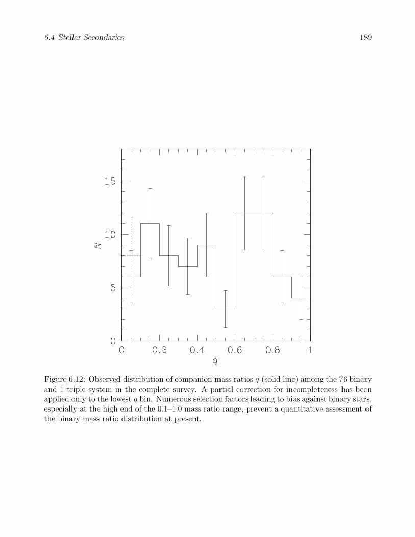
6.4 Stellar Secondaries 189
Figure 6.12: Observed distribution of companion mass ratios q (solid line) among the 76 binaryand 1 triple system in the complete survey. A partial correction for incompleteness has beenapplied only to the lowest q bin. Numerous selection factors leading to bias against binary stars,especially at the high end of the 0.1–1.0 mass ratio range, prevent a quantitative assessment ofthe binary mass ratio distribution at present.
Chapter 7
Discussion and Summary
In this final Chapter, we discuss the answer to the main question raised at the onset of thiswork: what is the frequency of wide sub-stellar companions to solar analogs? Our robuststatistical analysis of the results in §6 showed that, on average, 6.8% of 3–500 Myr-old Sun-likestars harbor 0.012–0.072 M brown-dwarf companions in semi-major axes between 30 AU and1600 AU. The 2σ (≈ 95%) confidence interval on this estimate is 1.9%–15.1%. How does thiscompare to the frequencies of sub-stellar companions found in other surveys? Are brown-dwarfsecondaries less common than extra-solar planets and stellar secondaries? Is the measuredfrequency consistent with a brown-dwarf desert at wide separations? The short answer to thelast question is “No.” For the reader seeking a more in-depth discussion, such is offered in §7.1and §7.2. Emphasis is placed on a comparison with the results from the survey of McCarthy& Zuckerman (2004)–the most similar in scope to the present one. Section §7.3 offers variousdirections for future research, and the final Section (§7.4) summarizes the results from the entirestudy.
7.1 Comparison to the Results of McCarthy & Zucker-
man (2004)
As already noted in §2.5.1, the only other direct imaging survey for sub-stellar companions thatis similar in scope and sensitivity to the present work is the survey of McCarthy & Zuckerman(2004), performed for C. McCarthy’s Ph.D. Thesis (McCarthy, 2001). The ensuing discussioncompares the two surveys in parallel detail.
Both surveys focus on young stars visible from the northern hemisphere. The McCarthy &Zuckerman (2004) survey is done at J band, with follow-up at I. Similarly to the present work(done at KS band), it consists of a deep (Keck) and a shallow (using 2.3–3 m Lick telescopes atLick and Steward observatories) imaging component, with a nearly identical distribution of thetargets between the two: 102 (deep) vs. 178 (shallow), compared to 101 (deep) vs. 165 (shallow)in this work. Unlike the present survey, the McCarthy & Zuckerman survey is seeing-limited,thus potentially of poorer contrast. In addition, McCarthy & Zuckerman use much wider(5–6′′) occulting spots, compared to the 1′′ coronagraph used here. Nevertheless, despite thedifferences in operating wavelength, contrast, and size of the occulting spot, the relative choicesof sample age and heliocentric distance of the two surveys are such that the claimed sensitivitiesto companion masses and the probed orbital separation ranges are remarkably similar. Bothsurveys are expected to be sensitive to companions as small as ∼ 5MJup around the nearest and
190

7.1 Comparison to the Results of McCarthy & Zuckerman (2004) 191
youngest sample stars, and cover projected separations in the approximate range ∼30–2000 AU.Yet, the results and conclusions are rather different. McCarthy & Zuckerman (2004) detect nobrown-dwarf companions, from which they infer that the brown-dwarf desert extends out to atleast 1200 AU from stars. We find a total of three sub-stellar companions and conclude theopposite (§7.2.2).
Taken at face value, without correcting for detection biases, a no-detection result in thepresent survey can be excluded at the 1 − e−3 = 0.95 confidence level, i.e., the two results are≈ 2σ discrepant. It is therefore remotely possible, though unlikely, that luck was unevenlydistributed between the two studies. However, the increasing rate of success of recent, higher-contrast surveys (§2.5.4), suggests otherwise. There are thus reasons to believe that McCarthy& Zuckerman (2004) may have under-estimated the incompleteness and/or age of their surveysample. I address these two possibilities in the following, by considering only the results fromMcCarthy & Zuckerman (2004)’s deep sample.
7.1.1 Completeness Estimate of the McCarthy & Zuckerman (2004)
Survey
McCarthy & Zuckerman (2004) quote typical detection limits for their imaging of ∆J =12.5 mag at >5′′ from their primaries and a typical sample age of 300 Myr. They use theseto infer that their survey is sensitive to sub-stellar companions down to the deuterium-burninglimit (12 MJup) around 97% of the stars, and down to 15 MJup around 100% of the stars ob-served at Keck. If “typical” in both cases is interpreted as “median,” then, by definition, theadopted values for their sensitivity limits and stellar age over-estimate the sensitivity of thesurvey and under-estimate the age of the sample in exactly half of the cases for each of the twoparameters. Therefore, the assumed incompleteness is correct only for ∼1/4 of their observa-tions, while for the remaining 3/4, the sensitivity is over-estimated to varying degrees. This canindeed be gleaned from several discussions in the McCarthy & Zuckerman (2004) paper, suchas the requirement that atmospheric transparency does not decrease the limiting magnitudebelow J = 19 mag (whereas a limiting magnitude of J ≥ 20 mag is assumed throughout), anda cursory mentioning of the fact that sensitivities were computed for a 10–1000 Myr range ofages (though the 300 Myr typical age is assumed in estimating the brown-dwarf companionfrequency). Because detections of sub-stellar companions made under the best contrast andat most favorable (i.e., youngest) stellar ages will generally be the ones governing the overallstatistics, an over-estimate of the sensitivity of a survey in the above manner will lead to fre-quency estimates that are too conservative. In the case of the McCarthy & Zuckerman (2004)survey, this is partially alleviated by the fact that they do not detect any sub-stellar com-panions, so there are no statistics to consider. However, the issues raised here will affect theminimum mass limits of the detectable sub-stellar companions. That is, the quoted minimummass limits by McCarthy & Zuckerman (2004) are likely too optimistic for the majority of theirobservations. As a result, contrary to what is claimed, the authors have been unable to probethe entire brown-dwarf regime down to the deuterium-burning limit, and their upper limit onthe frequency of brown-dwarf companions needs to be corrected for the fraction of the sub-stellar mass regime that is missed. For the present survey, this kind of incompleteness, termed“observational incompleteness,” was addressed in §6.2.3.2 by assuming a mass distribution forsub-stellar companions (checked against the one observed in our survey).
The McCarthy & Zuckerman (2004) analysis also does not take into account either of the

7.1 Comparison to the Results of McCarthy & Zuckerman (2004) 192
remaining two incompleteness terms discussed in §6.2.3: “geometrical,” arising from the lackof full coverage of the entire orbital range of interest around all sample stars, and “orbital”(or “SVOC”, following the terminology in Brown, 2004), resulting from the distribution oforbital parameters of the possible companions. Instead, the intrinsic assumption is of 100%completeness to all objects in the considered range of projected separations, and of face-on,circular orbits. As was found in §6.2.3 and as discussed in Brown (2004), the combined effect ofthese geometrical and the orbital incompleteness can be a factor of several for the lowest massobjects at the smallest separations from the effective obscuration.
Therefore, McCarthy & Zuckerman (2004) have probably over-stated the ensemble sensitiv-ity of their survey by a factor of several, thus artificially lowering their estimate of the upperlimit on the frequency of sub-stellar companions in wide orbits.
7.1.2 Age Estimate of the McCarthy & Zuckerman (2004) Sample
A likely reason for the lack of sub-stellar companion detections in McCarthy & Zuckerman(2004) altogether is that they may have over-estimated the youth of their sample. Around anolder set of stars, any sub-stellar companions will be dimmer, hence more challenging to detect.Thus, assuming a sample age that is too young will lead to deriving a sub-stellar companionfrequency that is too conservative. In the following discussion we address two reasons why theMcCarthy & Zuckerman (2004) sample may be older than the ∼300 Myr median age assumedby the authors.
7.1.2.1 A Space-motion Selected Sample Needs Independent Age Verification
The primary selection criterion for the McCarthy & Zuckerman parent sample is stellar spacemotion, following the original idea of Eggen (1965) that young stellar populations inhabita narrow region of (U, V,W ) velocity phase space in the Galaxy. Discoveries of nearby co-moving groups of stars (e.g., Webb et al., 1999; Mamajek et al., 1999; Zuckerman et al., 2001a),confirmed to be young through a combination of age-dating criteria (§2.2.2), have shown thatthis approach is a viable tool for identifying young stars. The particular regions of phasespace used by McCarthy & Zuckerman include the one presented in Eggen (1996, −30 < V <0,−25 < U < 50,−40 < W < 40 km s−1), which they apply to all single northern K and Mdwarfs in the Third Catalog of Nearby Stars (Gliese & Jahreiß, 1991), and the UVW regionidentified by Jeffries (1995, −30 < V < −20,−20 < U < 0,−20 < W < 20 km s−1), whichthey apply to all known single GKM stars within 25 pc. The latter, much narrower (4.4%of the UVW volume defined in Eggen, 1996) phase space includes a number of known youngkinematic associations: the ∼100 Myr-old Pleiades moving group, the ∼10 Myr-old TW Hyaassociation (Kastner et al., 1997), and the 8 Myr-old η Cha cluster (Mamajek et al., 1999).However, the larger phase space includes dwarfs as old as 2 Gyr (Eggen, 1996). Therefore theirparent sample may contain an appreciable fraction of Gyr-aged stars.
The authors do include a number of stars with youth established via other methods, includ-ing M dwarfs with strong Hα emission (Reid et al., 1995) and high x-ray luminosity (Fleming,1998; Appenzeller et al., 1998), K dwarfs with high Li I equivalent width (Fischer, 1998), G andK dwarfs with Ca II H&K emission (Soderblom et al., 1993), as well as known members of theTW Hya association. However, these are apparently included in addition to the UV W -selectedsample. That is, members of the latter have not undergone the same scrutiny for youth. With-

7.1 Comparison to the Results of McCarthy & Zuckerman (2004) 193
out consideration of additional age-dating criteria to confirm the youth of the kinematicallyselected stars, the true age distribution of the sample is unknown.
7.1.2.2 The McCarthy & Zuckerman (2004) Sample Is Statistically 1 Gyr Old
McCarthy & Zuckerman base their ∼300 Myr estimate for the median age of their sample on acombination of age-dating and statistical arguments. However, they do not list individual stellarages. Instead, they provide an independent check on the overall age distribution by comparingthe number of stars in their youth-selected sample that reside within 15 pc of the Sun to thenumber of ≤1 Gyr-old northern (δ > −30) stars estimated to be present in the Gliese Catalogin the same volume of space. In particular, they cite Rocha-Pinto et al. (2000a) in adopting that21% of surveyed stars in the solar neighborhood are younger than 1 Gyr. Hence, given theirestimate of ∼400 single northern Gliese stars within 15 pc of the Sun, McCarthy & Zuckerman(2004) find that ∼80 of these should be younger than 1 Gyr. By comparing this number tothe actual number of stars in their 15 pc sub-sample (102 for the Lick/Steward survey; 48 forthe Keck survey), the authors argue that they have selected most of the known nearby starsyounger than 1 Gyr.
However, the quoted fraction of 21% is an over-estimate of the fraction of ≤ 1 Gyr-old starsin the solar neighborhood. While indeed 21% of the G stars observed in the quoted surveyby Rocha-Pinto et al. (2000a) are classified as younger than 1 Gyr, that survey is not volume-complete. Rocha-Pinto et al.’s sample is flux-limited, extends out to 200 pc, and is thereforebiased toward younger (brighter) stars, e.g., members of several known <1 Gyr-old associationsat 40–200 pc from the Sun. Contrarily, very few members of such young associations are knownwithin 15 pc of the Sun (e.g., Zuckerman & Song, 2004a). Therefore, the age distributions ofRocha-Pinto et al.’s sample and of Gliese stars within 15 pc are distinct. Indeed, in a separatestudy of the star-formation history in a volume-complete sample of nearby (5–22 pc) M dwarfs,Gizis et al. (2002) find that only ∼9% of M dwarfs are younger than 1 Gyr (Fig. 12 in Giziset al., 2002). This result agrees with the completeness-corrected estimate of the local G-dwarfstar-formation rate in Rocha-Pinto et al. (2000b), who find that only ∼10% of stars formed inthe solar neighborhood are younger than 1 Gyr (Fig. 8 in Rocha-Pinto et al., 2000b). Bothstudies indicate a roughly uniform star-formation rate over the last 10 Gyr. Given that theGliese Catalog is nearly volume-complete out to 15 pc for spectral types earlier than ∼M4 (Reidet al., 1995), the fraction of <1 Gyr-old Gliese stars within 15 pc is, accordingly, 9–10%.
Following McCarthy & Zuckerman’s reasoning, we find that only 35–40 of the 102 stars intheir Lick/Steward 15 pc sub-sample are younger than 1 Gyr, rather than ∼80. In fact, assumingthat McCarthy & Zuckerman have managed to select the youngest quartile of the ∼400 suitableGliese stars within 15 pc, the Rocha-Pinto et al. (2000b) and Gizis et al. (2002) results implythat the stellar ages in this sub-sample should be approximately uniformly distributed between0 and 2.5 Gyr. Given that McCarthy & Zuckerman apply the same age-selection criteria to theirKeck sample, its age distribution is likely to be the same. This argues for a median sample ageof 1.25 Gyr for McCarthy & Zuckerman’s combined sample, rather than 300 Myr, as the authorsassume. In reality, after taking into account the UVW selection counter-argument describedin §7.1.2.1, most of the UVW -selected members of the McCarthy & Zuckerman (2004) samplethat do not belong to known kinematic groups of young stars are probably 1–10 Gyr old. Whilea number of bona fide young stars are included in their sample and they certainly dilute themedian age toward smaller values, overall the median sample age is unlikely to be <1 Gyr.

7.2 Comparison to Previous Multiplicity Results 194
7.1.3 Comparison of Sensitivities to Sub-stellar Companions
To compare the sensitivities of the two surveys, we use the median sample distances and ages tocalculate the minimum sub-stellar mass detectable at the respective survey wavelengths (1.2µmand 2.15µm). Although, as argued in §7.1.1, the use of median sample statistics is incorrect inestimating ensemble sensitivities, it should provide at least a cursory idea of the relative surveysensitivities.
Judging from the fact that approximately equal numbers of stars are contained within andoutside the 15 pc sub-sample of McCarthy & Zuckerman (2004), we adopt 15 pc as the medianheliocentric distance of their deep sample. Building on the arguments presented in §7.1.2, weadopt a median sample age of 1 Gyr for the McCarthy & Zuckerman (2004) stars, recognizinghowever that their sample also contains ∼20 bona fide 10–100 Myr-old confirmed members ofyoung kinematic groups. From the distribution of primary spectral types in their sample (Tab. 1in McCarthy & Zuckerman, 2004), we estimate a median spectral type of M0, corresponding toa mass of ≈ 0.50M (Cox, 2000, and references therein). Finally, we assume a typical limitingmagnitude of J = 20 for their Keck NIRC data, as determined by the authors.
Taking the above values into account, the minimum detectable object mass in the McCarthy& Zuckerman (2004) survey is ≈ 40MJup at median sample statistics. At a typical limitingmagnitude of KS = 19.5 mag for the coronagraphic component of the present survey (Fig. 5.3b),and median deep sample age and distance of 80 Myr and 50 pc, respectively, the minimumdetectable companion mass is 8–10 MJup–a factor of 4 smaller. Therefore, the higher successrate of the present survey, in comparison with that of McCarthy & Zuckerman (2004), doesnot come as a surprise. Note, however, that using 8–10 MJup as a “typical” sensitivity limit ofour survey leads to a gross overestimate the ensemble sensitivity, given that the completenessto such low masses is only 25–35% (Fig. 6.9a).
We therefore conclude that the 1 ± 1% upper limit on the sub-stellar companion frequencyquoted by McCarthy & Zuckerman (2004) is too conservative, probably by a factor of several.
7.2 Comparison to Previous Multiplicity Results
7.2.1 Other Direct Imaging Surveys for Sub-stellar Companions
Does the estimate for the brown-dwarf companion frequency in this survey agree with thosefound in other surveys?
The three previous large surveys that report at least one detection (Oppenheimer et al.,2001; Lowrance et al., 2005; Chauvin et al., 2005b) produce results that are consistent with thepresent rate of success (3/101) at least at the 2σ. This comparison does not take into accountthe differences in the probed separation ranges and survey completeness. The detection ratesfor the surveys are 1/164, 2/45, and 1/50, respectively, with the Oppenheimer et al. (2001)survey (performed with only low-order tip-tilt AO at the Palomar 1.5 m telescope) being leastsensitive, and covering the smallest orbital separation range (10–100 AU). A rough comparisonof the various degrees of sensitivity and completeness indicates that the probable correctionfactors will make the incompleteness-corrected estimates in all cases fully consistent with theone presented here. Naturally, smaller surveys, reporting at least one detection (Potter et al.,2002; Neuhauser & Guenther, 2004, success rates of 1/31 and 1/25, respectively), also produceresults that are highly consistent with the present one.

7.2 Comparison to Previous Multiplicity Results 195
High-contrast surveys that do not detect sub-stellar companions (other than that of Mc-Carthy & Zuckerman (2004)) are published in Schroeder et al. (2000, 23 stars), Brandner et al.(2000, 24 stars), Masciadri et al. (2005, 28 stars), Carson et al. (2005, 80 stars), and Luhmanet al. (2005, 150 stars). The samples of the first three surveys are far too small for meaningfulcomparison, given the expected low detection success rates. The Carson et al. (2005) surveyhas poorer sensitivity to sub-stellar masses than the present survey, because it targets 1–10 Gyrstars in the solar neighborhood. A detailed Monte Carlo analysis by Carson et al. (2004) showsthat, despite the null detection result, brown-dwarf companion frequencies as high as 9.7%cannot be excluded. Finally, the Luhman et al. (2005) survey is very sensitive to sub-stellarmasses, as it is performed with HST/WFPC2 and targets the very young (2 Myr) star-formingregion IC 348. It also probes a very similar range of projected separations (120–1600 AU), tothe one probed here (22–1260 AU). The non-detection of sub-stellar companions by Luhmanet al. may therefore appear puzzling. However, the Luhman et al. result needs to be consideredin the context of the mass distribution of their sample stars.
The vast majority of the Luhman et al. targets are in the 0.08–0.5 M mass range, withonly 29 stars in the 0.5–1.5 M range (i.e., similar to the mass range explored in the presentsurvey). The non-detection of companions around the 29 higher-mass stars is not surprising,given the small size of the sub-sample. The lack of detections around the lower-mass stars, onthe other hand, may be an indication that lower-mass primaries cannot retain wide companions.Such a mass-dependent effect has already been reported in the companion survey of ≈0.1 Mprimaries by Close et al. (2003). Close et al. observe that the distribution of orbital separationsin very low mass binaries (total mass ≤ 0.19M) peaks at 4 AU and cuts off after 16 AU. Theauthors reason that dynamical perturbations by passing stars disrupt the shallow potentialwells of wide very low-mass binaries, leading to the preferential survival of the hardest systems.Because the majority of the primaries in the Luhman et al. (2005) sample are of similarly lowmass, and because of the relatively large heliocentric distance of IC 348 (315 pc), the majorityof the binary systems in the Luhman et al. sample would span ≤ 0.05′′ and would not have beenresolved. The non-detection of sub-stellar companions by Luhman et al. (2005) is thus probablydue to the low mean mass of their sample and to the dependence of the binary semi-major axisdistribution on total mass.
The above interpretation is also in line with the decreasing incidence of q ≤ 0.2 systemsamong resolved binaries from early-type (B–A) stars (35–40%; Tokovinin et al., 1999; Shatsky& Tokovinin, 2002; Kouwenhoven et al., 2005), to G–K dwarfs (10–20%; Duquennoy & Mayor,1991), and to M8–L0 dwarfs (0%; Close et al., 2003). Binary systems, consisting of a late-type(K–M) primary and a sub-stellar secondary have mass ratios q . 0.2. In the context of adecreasing frequency of such systems toward later spectral types, the absence of sub-stellarcompanions around late-type stars is not surprising. Volume-limited surveys (Oppenheimeret al., 2001), or other surveys dominated by K and M dwarf primaries (McCarthy & Zuckerman,2004; Luhman et al., 2005), will be expected see a brown-dwarf desert at wide separations.
An alternative hypothesis, that could also explain the lower success rate of direct imagingsurveys for sub-stellar companions targeting 1–10 Gyr-old stars, is evolution of the sub-stellarcompanion frequency. Evolution in the occurrence rate of stellar binaries between the agesof ∼1 Myr-old star-forming regions and of 1–10 Gyr-old solar neighborhood stars is a well-documented effect, with the binary frequency dropping by a factor of 2 between the ages ofthese two stellar populations (Duquennoy & Mayor, 1991; Ghez et al., 1993, 1997; Kohler &Leinert, 1998; Patience et al., 2002). If this process is due to the dynamical disruption of wider
7.3 Future Directions 196
binaries by passing stars, it seems plausible that the same effect could be responsible for the“disappearance” of low-mass companions around older stars.
We therefore conclude, that while the present imaging survey has one of the highest pub-lished success rates of sub-stellar companion detection, the obtained results are not inconsist-nent with those of other teams, given appropriate consideration of survey incompleteness ineach case. Instead, the higher success rate is a direct result of an appropriately-selected sampleof young stars, and ability to attain high imaging contrast. The McCarthy & Zuckerman (2004)claim that wide brown-dwarf companions to young stars occur in only 1 ± 1% of cases can berefuted at the > 2σ level.
7.2.2 Comparison to Planetary and Stellar Multiplicity: No BrownDwarf Desert at >30 AU from Solar Analogs
The brown-dwarf desert at 0–3 AU semi-major axes (the present completeness limit of RVsurveys) is defined with respect to the observed frequencies of extra-solar planets (5–15%;Marcy & Butler, 2000; Fischer et al., 2002) and stellar companions (11%; Duquennoy & Mayor,1991) around Sun-like stars in the same semi-major axis range. The frequency of brown dwarfsin such orbits is <0.5% (Marcy & Butler, 2000)–a factor of ∼20 lower than that of eitherplanetary or stellar companions. This ratio we adopt as a quantitative definition for the term“brown-dwarf desert.”
The wider, 30–1600 AU, semi-major axes probed around solar analogs in the present surveyprevent a comparison with the RV planet regime. The frequency of stellar companions over thissemi-major axis range is estimated to be ≈22%, based on the Duquennoy & Mayor (1991) perioddistribution. Our inferred frequency of brown dwarfs is 6.8%–a factor of 3 smaller. If we considerthe inferred companion frequencies per logarithmic mass interval, recognizing the narrower massrange spanned by brown dwarfs in comparison to ≤ 1M stars, the 0.012–0.072Msub-stellarcompanion frequency becomes 8.7% per unit of logM–a factor of 2.5 less than that for 0.1–1.0M stellar companions. A difference in the sub-stellar and stellar companion frequencies bya factor of 20, as in the RV brown-dwarf desert, is excluded at the ≈99% confidence level. Giventhat the ratio between the frequencies of brown-dwarf and stellar companions has increased bynearly an order of magnitude between 0–3 AU and the wide orbital separations probed here,we consider “desert” to be an incorrect term. Nevertheless, a deficiency may exist.
7.3 Future Directions
This work has focused exclusively on young stars, because of the advantage that they offer indirect imaging searches for sub-stellar secondaries. However, this far from exhausts the scientificinterest in studying sub-stellar companions to young stars. In addition to being suitable hostsfor the imaging of brown-dwarf companions, young stellar/sub-stellar systems are also goodchronometers for tracing brown-dwarf evolution. While a number of age-dating techniquesexist for hydrogen-burning stars (e.g, §2.2.2), brown-dwarf ages are much harder to constrain,because of the degeneracy between effective temperature and mass. Given an independent ageestimate from a primary stellar companion, the interplay between these three quantities canbe easily determined. Measurements of surface gravity and effective temperatures from low-resolution spectroscopy can then be accurately placed in evolutionary context. This provides

7.3 Future Directions 197
both a test for brown-dwarf cooling models and a reference point for the empirical calibrationof a much larger body of isolated sub-stellar objects.
This is of particular interest for the study of young and cool sub-stellar objects, none ofwhich are known at a spectral type later than L7. On one hand, such brown dwarfs areinteresting, because they may have masses similar to those of known extra-solar planets. Theircharacterization can thus offer much-needed insight into the mechanisms that govern planetand low-mass brown-dwarf formation. On the other hand, such brown dwarfs can be used totrace evolution in brown-dwarf photospheres. For example, brown dwarfs of known ages nearthe L/T spectral type transition can provide a direct estimate of the lifetime of dust grains insub-stellar photospheres prior to grain condensation.
This latter issue will be addressed in the immediate future. The coolest of the three detectedbrown dwarfs, HD 203030B, at a photometrically-estimated spectral type of T0 and an age of∼400 Myr, is likely to be the first young L/T transition object observed. Low-resolution near-IRspectra already at hand will be used to confirm this, as well as to obtain a measurement of thesub-stellar gravity. HD 203030B will thus offer the first empirical glimpse into the photospheresyoung T dwarfs.
Looking beyond companion statistics and photospheres of brown dwarfs, the stellar mul-tiplicity and astrometric results from the present study will be combined with results fromprevious imaging campaigns and from on-going RV monitoring of a sub-sample of the starsto obtain accurate dynamical masses. This will fill a presently sparsely-populated area in ourknowledge of dynamical stellar masses at young ages. The superior power of combining as-trometric and RV data in estimating dynamical masses was already employed in the orbitalcalculation for HD 129333A/B in §3.3.4.3. The idea is certainly extendable to sub-stellar massesthrough astrometric monitoring with the Space Interferometry Mission (SIM), which will usherin a new era of precise knowledge of sub-stellar masses.
Finally, high-contrast imaging of young stars has only just taken off the ground as an effec-tive technique to detect both candidate extra-solar planets and scattered light from the circum-stellar disks that they may be embedded in. Recent detections of planetary-mass companionswith AO (Chauvin et al., 2004, 2005a; Neuhauser et al., 2005), and high-contrast imaging stud-ies of debris disks with AO (Liu et al., 2004, Metchev et al., 2005: Appendix A) and HST(Krist et al., 2005; Kalas et al., 2005), have pre-viewed the scientific gains to be expected in thefields of extra-solar planets and planet formation the next few years. Ground-based AO capa-bilities are fast improving with the increasing availability of laser guide stars (Lick, Palomar,Keck), near-IR wavefront sensors (VLT), sensitive high-order AO systems (AEOS, Palomar,Keck, VLT), and interferometric baselines (Keck, VLT). These are being followed closely bythe implementation of novel contrast-enhancing detection techniques, based on optimized coro-nagraphy (e.g., Sivaramakrishnan et al., 2001; Kasdin et al., 2003), simultaneous differentialimaging at multiple bandpasses (Close et al., 2005; Marois et al., 2005) and polarizations (Apaiet al., 2004). In combination with the present-day sensitivity of Spitzer and of the HST, thesetechnological advances are bound to push the envelope of our knowledge of extra-solar plan-etary systems in preparation for the detection and direct imaging of Earth-like planets, withSIM and the Terrestrial Planet Finder.

7.4 Summary 198
7.4 Summary
We have presented results from an adaptive optics survey conducted with the Palomar and Kecktelescopes over 3 years, aimed at measuring the frequency of stellar and sub-stellar companionsto Sun-like stars. The survey sample contains 266 stars in the 3 Myr–10 Gyr age range at helio-centric distances between 8 and 200 parsecs and spectral types between F5–K5. A sub-sampleof 101 stars, between 3 and 500 Myr old, was observed in deep exposures with a coronagraph tosearch for faint sub-stellar companions. A total of 288 candidate companions were discoveredaround the sample stars, which were re-imaged at subsequent epochs to determine physicalassociation with the candidate host stars by checking for common proper motion. Benefitingfrom a highly-accurate astrometric calibration of the observations, we were able to successfullyapply the common proper motion test in the majority of the cases, including stars with propermotions as small as 20 milli-arcseconds year−1.
The results from the survey include the discovery of three new brown-dwarf companions,HD 49197B, HD 203030B, and ScoPMS 214B, 43 new stellar binaries, and a triple system.The physical association of an additional, a priori suspected, candidate sub-stellar companionto the star HII 1348 is astrometrically confirmed. The newly-discovered and confirmed youngbrown-dwarf companions span a range of spectral types between M5 and T0 and will be ofprime significance for constraining evolutionary models of young brown dwarfs and extra-solarplanets.
Based on the 3 new detections of sub-stellar companions in the 101 star sub-sample, andfollowing a careful estimate of the survey incompleteness, a Bayesian statistical analysis showsthat the frequency of 0.012–0.072 solar-mass brown dwarfs in 30–1600 AU orbits around youngsolar analogs is 6.8+8.3
−4.9% (2σ limits). While this is a factor of 3 lower than the frequencyof stellar companions to G-dwarfs in the same orbital range, it is significantly higher thanthe frequency of brown dwarfs in 0–3 AU orbits, discovered through precision radial velocitysurveys. It is also fully consistent with the observed frequency of 0–3 AU extra-solar planets.Thus, the result demonstrates that the radial-velocity “brown-dwarf desert” does not extendto wide separations, contrary to previous belief.

Appendix A
Adaptive Optics Imaging of the AUMicroscopii Circumstellar Disk: Evidence forDynamical Evolution
†Stanimir A. Metcheva, Lynne A. Hillenbranda, Joshua A. Eisnera, & SebastianWolfb
aCalifornia Institute of Technology, Division of Physics, Mathematics & Astronomy, MC 105–24, Pasadena,California 91125
bMax-Planck-Institut fur Astronomie, Konigstuhl 17, D–69117 Heidelberg, Germany
Abstract
We present an H-band image of the light scattered from circumstellar dust around the nearby(10 pc) young M star AU Microscopii (AU Mic, GJ 803, HD 197481), obtained with the Keckadaptive optics system. We resolve the disk both vertically and radially, tracing it over 17–60 AU from the star. Our AU Mic observations thus offer the possibility to probe at high spatialresolution (0.04′′ or 0.4 AU per resolution element) for morphological signatures of the debrisdisk on Solar-System scales. Various sub-structures (dust clumps and gaps) in the AU Mic diskmay point to the existence of orbiting planets. No planets are seen in our H-band image downto a limiting mass of 1 MJup at >20 AU, although the existence of smaller planets can notbe excluded from the current data. Modeling of the disk surface brightness distribution at H-band and R-band, in conjunction with the optical to sub-millimeter spectral energy distribution,allows us to constrain the disk geometry and the dust grain properties. We confirm the nearlyedge-on orientation of the disk inferred from previous observations and deduce an inner clearingradius ≤10 AU. We find evidence for a lack of small grains in the inner (<60 AU) disk, either asa result of primordial disk evolution or because of destruction by Poynting-Robertson and/orcorpuscular drag. A change in the power-law index of the surface brightness profile is observednear 33 AU, similar to a feature known in the profile of the β Pic circumstellar debris disk.By comparing the time scales for inter-particle collisions and Poynting-Robertson drag betweenthe two systems, we argue that the breaks are linked to one of these two processes.
†A version of this appendix was published in The Astrophysical Journal, vol. 622, 451
199

A.1 Introduction 200
A.1 Introduction
The existence of dust disks around main-sequence stars has been known since the first daysof the Infrared Astronomy Satellite (IRAS) mission, when Aumann et al. (1984) reported thedetection of strong far-infrared (far-IR) excess emission toward Vega (α Lyr). Over 200 othermain-sequence stars have since been reported to possess such excesses, found almost exclusivelywith IRAS and the Infrared Space Observatory (e.g., Backman & Paresce, 1993; Mannings &Barlow, 1998; Silverstone, 2000; Habing et al., 2001; Spangler et al., 2001; Laureijs et al., 2002;Decin et al., 2003), though recently also with Spitzer (e.g., Meyer et al., 2004; Gorlova et al.,2004), and through ground-based sub-millimeter observations (Carpenter et al., 2004). Too oldto possess remnant primordial dust, which would be cleared by radiation pressure and Poynting-Robertson (P-R) drag within several million years (Myr) in the absence of gas, these stars owetheir far-IR excess to emission by “debris disks,” formed by the collisional fragmentation oflarger bodies (the so-called “Vega phenomenon”; Backman & Paresce, 1993, and referencestherein). Subsequent imaging at optical to millimeter wavelengths of the nearest sub-sample ofVega-like stars has resolved intricate disk-like structures, with gaps and concentrations (Hollandet al., 1998, 2003; Greaves et al., 1998; Schneider et al., 1999; Krist et al., 2000; Koerner et al.,2001; Wilner et al., 2002; Weinberger et al., 2002; Clampin et al., 2003).
The most favored explanation for such structures is the gravitational perturbation by embed-ded planets orbiting at semi-major axes comparable to the disk size (Moro-Martın & Malhotra,2002; Kenyon & Bromley, 2004). The existence of perturbing planets may be revealed by clumpsof dust trapped in mean motion resonances, as has been suggested for Vega (Wilner et al., 2002;Wyatt, 2003), ε Eri (Ozernoy et al., 2000; Quillen & Thorndike, 2002), and Fomalhaut (α PsA;Wyatt & Dent, 2002; Holland et al., 2003), and observed by the Cosmic Background Explorersatellite along the Earth’s orbit (Reach et al., 1995). Stochastic collisions between large plan-etesimals that result in dust clumps lasting several hundreds of orbital periods are anothermeans of producing disk asymmetries (Stern, 1996). Spiral density waves (as seen in the disk ofHD 141569A, and inferred around β Pic; Clampin et al., 2003; Kalas et al., 2000) and warps inthe disk inclination (as in the disk of β Pic; Heap et al., 2000; Wahhaj et al., 2003) may indicateperturbation by nearby stars (Kalas et al., 2000, 2001; Kenyon & Bromley, 2002; Augereau &Papaloizou, 2004). Finally, dust migration in a gas-rich disk can produce azimuthally sym-metric structures, as observed in the HR 4796A circumstellar disk (Takeuchi & Artymowicz,2001).
High-resolution imaging observations, such as those of HR 4796A (Schneider et al., 1999),β Pic (Heap et al., 2000), HD 141569A (Weinberger et al., 1999) and TW Hya (Krist et al.,2000; Weinberger et al., 2002) with the Hubble Space Telescope (HST) can help single outthe most likely physical process behind the disk morphology. The resolution achievable withadaptive optics in the near-infrared on large ground-based telescopes rivals that of HST and isthe method employed in this paper for investigating disk structure.
The young (8–20 Myr; Barrado y Navascues et al., 1999; Zuckerman et al., 2001b) M1 V(Keenan, 1983) star AU Mic has a known 60µm excess from IRAS, likely due to orbiting dust(Song et al., 2002). Because of its relative proximity (Hipparcos distance of 9.94±0.13 pc;Perryman et al., 1997), AU Mic is a good target for high-resolution imaging of scattered lightto characterize the circumstellar disk morphology. Recent 450µm and 850µm observations byLiu et al. (2004) confirmed the existence of dust, and follow-up R-band (0.65µm) coronagraphicimaging revealed a nearly edge-on disk extending 210 AU (Kalas et al., 2004) from the star.
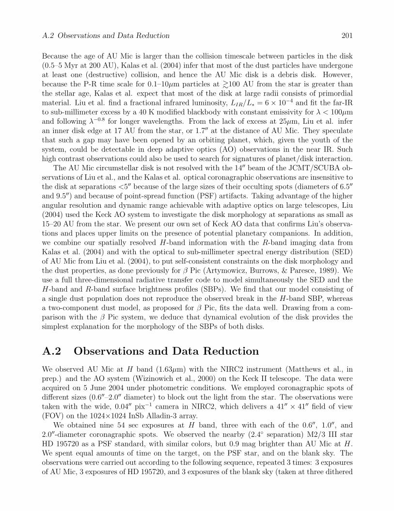
A.2 Observations and Data Reduction 201
Because the age of AU Mic is larger than the collision timescale between particles in the disk(0.5–5 Myr at 200 AU), Kalas et al. (2004) infer that most of the dust particles have undergoneat least one (destructive) collision, and hence the AU Mic disk is a debris disk. However,because the P-R time scale for 0.1–10µm particles at &100 AU from the star is greater thanthe stellar age, Kalas et al. expect that most of the disk at large radii consists of primordialmaterial. Liu et al. find a fractional infrared luminosity, LIR/L∗ = 6 × 10⁻⁴ and fit the far-IRto sub-millimeter excess by a 40 K modified blackbody with constant emissivity for λ < 100µmand following λ−0.8 for longer wavelengths. From the lack of excess at 25µm, Liu et al. inferan inner disk edge at 17 AU from the star, or 1.7′′ at the distance of AU Mic. They speculatethat such a gap may have been opened by an orbiting planet, which, given the youth of thesystem, could be detectable in deep adaptive optics (AO) observations in the near IR. Suchhigh contrast observations could also be used to search for signatures of planet/disk interaction.
The AU Mic circumstellar disk is not resolved with the 14′′ beam of the JCMT/SCUBA ob-servations of Liu et al., and the Kalas et al. optical coronagraphic observations are insensitive tothe disk at separations <5′′ because of the large sizes of their occulting spots (diameters of 6.5′′
and 9.5′′) and because of point-spread function (PSF) artifacts. Taking advantage of the higherangular resolution and dynamic range achievable with adaptive optics on large telescopes, Liu(2004) used the Keck AO system to investigate the disk morphology at separations as small as15–20 AU from the star. We present our own set of Keck AO data that confirms Liu’s observa-tions and places upper limits on the presence of potential planetary companions. In addition,we combine our spatially resolved H-band information with the R-band imaging data fromKalas et al. (2004) and with the optical to sub-millimeter spectral energy distribution (SED)of AU Mic from Liu et al. (2004), to put self-consistent constraints on the disk morphology andthe dust properties, as done previously for β Pic (Artymowicz, Burrows, & Paresce, 1989). Weuse a full three-dimensional radiative transfer code to model simultaneously the SED and theH-band and R-band surface brightness profiles (SBPs). We find that our model consisting ofa single dust population does not reproduce the observed break in the H-band SBP, whereasa two-component dust model, as proposed for β Pic, fits the data well. Drawing from a com-parison with the β Pic system, we deduce that dynamical evolution of the disk provides thesimplest explanation for the morphology of the SBPs of both disks.
A.2 Observations and Data Reduction
We observed AU Mic at H band (1.63µm) with the NIRC2 instrument (Matthews et al., inprep.) and the AO system (Wizinowich et al., 2000) on the Keck II telescope. The data wereacquired on 5 June 2004 under photometric conditions. We employed coronagraphic spots ofdifferent sizes (0.6′′–2.0′′ diameter) to block out the light from the star. The observations weretaken with the wide, 0.04′′ pix−1 camera in NIRC2, which delivers a 41′′ × 41′′ field of view(FOV) on the 1024×1024 InSb Alladin-3 array.
We obtained nine 54 sec exposures at H band, three with each of the 0.6′′, 1.0′′, and2.0′′-diameter coronagraphic spots. We observed the nearby (2.4 separation) M2/3 III starHD 195720 as a PSF standard, with similar colors, but 0.9 mag brighter than AU Mic at H .We spent equal amounts of time on the target, on the PSF star, and on the blank sky. Theobservations were carried out according to the following sequence, repeated 3 times: 3 exposuresof AU Mic, 3 exposures of HD 195720, and 3 exposures of the blank sky (taken at three dithered

A.2 Observations and Data Reduction 202
positions: 60′′, 50′′, and 40′′ away from the PSF star). The total on-source exposure time was8.1 min. Throughout the observations, the field rotator was set in “position angle mode,”preserving the orientation of the sky on the detector. The image quality was estimated fromthe Strehl ratios of point sources observed at higher spatial resolution (with the narrow camera,0.01′′/pix) at the beginning of each night. Our H band images had Strehls of 17–20%.
Data reduction followed the standard steps of sky-subtraction, flat-fielding, and bad-pixelcorrection. The images in the individual sets of 3 exposures were then median-combined toimprove the sensitivity to faint objects. The AU Mic dust disk was barely discernible at thisstage (Figure A.1a). To enhance the visibility of the dust disk, we subtracted the stellar PSF.The PSF was obtained by first rotating the image of HD 195720 to match the orientation of thediffraction pattern in the AU Mic image, and then scaling it by a centrally symmetric functionf(r) to match the radial dependence of the AU Mic profile. The objective of the scaling wasto compensate for variations in the seeing halo between AU Mic and the control star caused bychanging atmospheric conditions and fluctuating quality of the AO correction. The functionf(r) was obtained as the median radial profile of the ratio of the AU Mic to the HD 195720images, with the telescope spikes and the edge-on disk masked. Figure A.2 shows f(r) for theimages with the three different coronagraphic spot sizes. Two remarks on this procedure shouldbe made here. First, the function f(r) does not vary by more than 15% for any given spotsize and for large radii tends to 0.4—the H-band flux ratio between AU Mic and the PSF star.Second, because the AU Mic disk happens to be edge-on, the centrally symmetric scaling of thePSF does not introduce any spurious features in the result and so does not interfere with themorphology of the disk. The procedure would not be viable for disks that are far from edge-on.
The scaled version of HD 195720 for the image with the 0.6′′ coronagraph is presented inFigure A.1b. Panel (c) of Figure A.1 shows the final AU Mic image, obtained by median-combining all coronagraphic exposures. In panel (d) a digital mask has been employed toenhance the appearance of the circumstellar disk. The mask encompasses the innermost 1.7′′
from AU Mic, as well as the hexagonal diffraction spikes from 2 of the 3 image sequences wherethey did not subtract well (as seen in panel (c) of the Figure).
For flux calibration we adopted the 2MASS magnitude for AU Mic (H = 4.831 ± 0.016)and relied on the residual transmission of the NIRC2 coronagraphic spots. The PSF star,HD 195720, is saturated in 2MASS and is therefore unusable for flux calibration. We measuredthe flux from AU Mic through the 1.0′′ and 2.0′′ coronagraphs in a 6 pix (0.24′′) diameter aper-ture. From non-coronagraphic images taken with the 10 mas/pix camera on NIRC2, we foundthat this aperture contained 68% of the total power in the PSF. The H-band transmissivity ofthe 2′′ NIRC2 coronagraph was measured at (7.32±0.24)×10−4 (extinction of 7.84±0.03 mag).AU Mic is known to exhibit a large V -band photometric amplitude (0.35 mag) due to star spotswith a period of 4.9 days (Torres & Ferraz Mello, 1973). Although we do not expect measur-able variability over the ≈1 hour time span of our observations, our absolute flux calibration isuncertain. Nevertheless, in the near IR the contrast between the spots and the stellar photo-sphere is less pronounced than in the optical, so the uncertainty is also smaller—likely of order.0.1 mag.
The absolute orientation of the dust disk arms was calibrated through observations of abinary star standard, WDS 18055+0230, with well-known orbital elements (grade 1; Hartkopf& Mason, 2003; Pourbaix, 2000). The y-axis of the NIRC2 detector was measured to be offsetby 1.24 ± 0.10 clockwise from north. All position angles quoted below have been correctedfor this offset.

A.2 Observations and Data Reduction 203
AU Mic
(a)N
E
2" HD 195720
(b) N
E
AU Mic
(c)
AU Mic
(d)
Figure A.1: H-band images of AU Mic. (a) A median-combined image of three sky-subtracted54.3 sec exposures with the 0.6′′ coronagraph. The star is visible through the semi-transparentcoronagraph. The disk is discernible as a faint pair of diametrically opposite spikes along theSE–NW direction (traced by the two pairs of parallel lines). (b) An image of the PSF star,HD 195720, with the same coronagraph, scaled to the intensity of the AU Mic image in panel(a). An arrow points to the location of a faint projected companion (§A.3.3). (c) The finalmedian-combined image of AU Mic obtained from PSF-subtracted images with 0.6′′, 1.0′′, and2.0′′ spot diameters. All surface brightness photometry is performed on this image. (d). Sameas in (c), but with an overlaid digital mask covering the star and the telescope diffractionpattern. The residual noise in the central region (3.4′′-diameter circle) is greater than thesurface brightness of the edge-on disk.
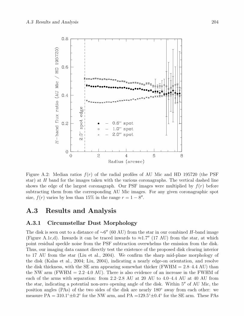
A.3 Results and Analysis 204
Figure A.2: Median ratios f(r) of the radial profiles of AU Mic and HD 195720 (the PSFstar) at H band for the images taken with the various coronagraphs. The vertical dashed lineshows the edge of the largest coronagraph. Our PSF images were multiplied by f(r) beforesubtracting them from the corresponding AU Mic images. For any given coronagraphic spotsize, f(r) varies by less than 15% in the range r = 1 − 8′′.
A.3 Results and Analysis
A.3.1 Circumstellar Dust Morphology
The disk is seen out to a distance of ∼6′′ (60 AU) from the star in our combined H-band image(Figure A.1c,d). Inwards it can be traced inwards to ≈1.7′′ (17 AU) from the star, at whichpoint residual speckle noise from the PSF subtraction overwhelms the emission from the disk.Thus, our imaging data cannot directly test the existence of the proposed disk clearing interiorto 17 AU from the star (Liu et al., 2004). We confirm the sharp mid-plane morphology ofthe disk (Kalas et al., 2004; Liu, 2004), indicating a nearly edge-on orientation, and resolvethe disk thickness, with the SE arm appearing somewhat thicker (FWHM = 2.8–4.4 AU) thanthe NW arm (FWHM = 2.2–4.0 AU). There is also evidence of an increase in the FWHM ofeach of the arms with separation: from 2.2–2.8 AU at 20 AU to 4.0–4.4 AU at 40 AU fromthe star, indicating a potential non-zero opening angle of the disk. Within 5′′ of AU Mic, theposition angles (PAs) of the two sides of the disk are nearly 180 away from each other: wemeasure PA = 310.1±0.2 for the NW arm, and PA =129.5±0.4 for the SE arm. These PAs

A.3 Results and Analysis 205
are in agreement with those reported in Liu (2004, 311.4±1.0 and 129.3±0.8), though theyare more accurate, likely as a result of our proper calibration of the orientation of the NIRC2detector (§A.2).
The radial SBP of the disk was measured on the reduced image (Figure A.1c; before applyingthe digital mask) using the IRAF task polyphot. The photometry regions are indicated bythe rectangles overlapped onto a contour map of the image in Figure A.3a. We used 4 pix ×12 pix (0.16′′ × 0.48′′) rectangular apertures, where the long side of the rectangular regionswas chosen to span 1–2 FWHMs of the disk thickness and was aligned normally to the diskarm. The distance between the aperture centers was 4 pix (0.16′′). Even though the image wasPSF- and sky-subtracted, to offset for flux biases introduced by the centrally symmetric scalingof the PSF (§A.2), we employed additional background subtraction, with the background fluxestimated as the median pixel value in 0.16′′-wide concentric annuli centered on the star. Thephotometric uncertainty was estimated as the quadrature sum of the standard deviation of thebackground and the photon noise from the disk. For the standard deviation of the backgroundwe adopted the root mean square (r.m.s.) of the pixel values in the annulus, multiplied by√
π/2 (to properly account for the standard deviation of the median; Kendall & Stuart, 1977)and normalized by the size of the photometry aperture.
The radial SBPs of the NW (upward pointing triangles) and SE (downward pointing trian-gles) arms of the projected disk are shown in Figure A.4. The two SBPs agree well throughoutthe region over which we can trace the disk (17–60 AU). Unlike the observed shape of theR-band SBP at 50–210 AU, the H-band SBP at 17–60 AU from the star cannot be fit by asingle power law. Instead, the SBPs of both the NW and the SE arms “kink” and flatteninwards of 30–40 AU, with the transition being more abrupt in the SE arm at ≈33 AU, andmore gradual in the NW arm. While the power-law exponent of the mean SBP over the entirerange (17–60 AU) is −2.3± 0.2, over 17–33 AU separations it flattens to −1.2± 0.3, while over33–60 AU, it increases to −4.0±0.6. These are consistent with the measurements of Liu (2004)over the same separation range.
A closer look at the SBP of the NW and SE arms reveals several small-scale asymmetries, allof which can be linked to regions of non-uniform brightness in the AU Mic disk (Figure A.3a).The sub-structure is enhanced by scaling the reduced image by a radially symmetric functioncentered on the star, with magnitude proportional to the radius squared (Figure A.3b). Thelettered structures denote features identified in the (deeper) image of Liu (2004): clumps ofenhanced emission (A, and C), a gap (B), and a region elevated with respect to the innerdisk mid-plane (D). In general, we confirm the presence of these features in the AU Mic disk,although the gap (B) and the clump (A) appear misplaced by ∼5 AU toward the star in ourimage. The NW arm also looks more uniform in brightness between 17–40 AU in our imagecompared to that in Liu (2004, Figures 3 and 4), where clump A is very prominent. Thesediscrepancies may be caused by residual speckle noise from the PSF subtraction in either dataset. In addition to the features described by Liu, we see a faint clump in the NW arm at &50 AUfrom the star, coincident with the location of the bump in the SBP of this arm (Figure A.4).The concentration is not reported by Liu and, being at a relatively low signal-to-noise (≈3),may be a noise spike.

A.3 Results and Analysis 206
(a)
E N
B
DC AA
(b)
(c)
Figure A.3: 12.0′′× 4.0′′ images of the AU Mic disk, with the SE arm oriented horizontally. (a)Locations of the photometry regions for measuring the disk surface brightness superimposed onthe final, masked image of AU Mic. The regions are 0.16′′ × 0.48′′ and sample 1–2 FWHMs ofthe disk thickness. The circular mask is 2′′ in radius. The crossed arrows mark the location ofAU Mic. The contour levels trace surface brightness from 17.5 mag arcsec−2 to 14.3 mag arcsec−2
in steps of 0.8 mag arcsec−2. (b) Small-scale structure in the AU Mic disk. The capital letterscorrespond to sub-structures identified by Liu (2004). The bar at the bottom is 10′′ (100 AU)long, extending from −50 AU to +50 AU along the disk plane, with tick marks every 10 AU.To enhance the appearance of the clumps in the disk, we have multiplied the pixel values bythe square of the distance from the star. The contour levels follow a squared intensity scale. (c)The preferred scattered light model of the AU Mic disk at H-band, created using the MC3Dcode (§A.4; Table A.1). The same software mask as in the other two panels has been applied.The contour levels follow the same spacing as in panel (a). No background noise is added,though Poisson-noise “clumps” due to low signal-to-noise of the model can be seen. These donot represent discrete physical structures.
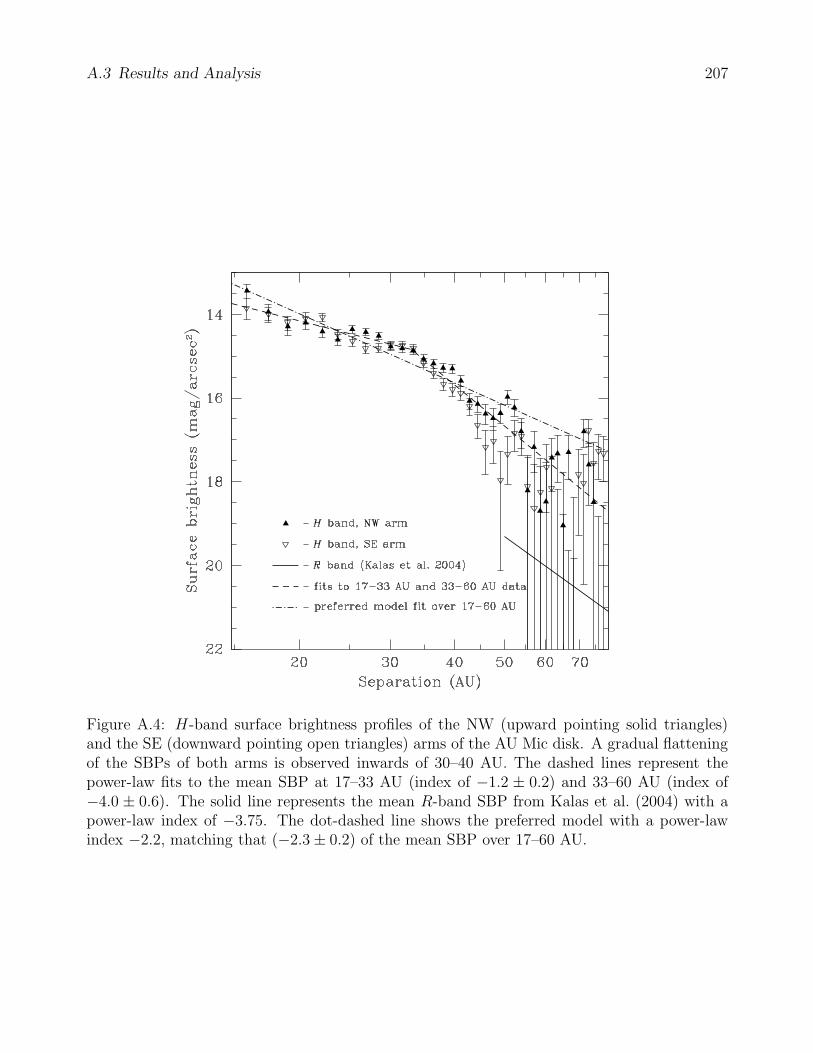
A.3 Results and Analysis 207
Figure A.4: H-band surface brightness profiles of the NW (upward pointing solid triangles)and the SE (downward pointing open triangles) arms of the AU Mic disk. A gradual flatteningof the SBPs of both arms is observed inwards of 30–40 AU. The dashed lines represent thepower-law fits to the mean SBP at 17–33 AU (index of −1.2 ± 0.2) and 33–60 AU (index of−4.0 ± 0.6). The solid line represents the mean R-band SBP from Kalas et al. (2004) with apower-law index of −3.75. The dot-dashed line shows the preferred model with a power-lawindex −2.2, matching that (−2.3 ± 0.2) of the mean SBP over 17–60 AU.

A.3 Results and Analysis 208
A.3.2 Disk Luminosity, Optical Depth, and Geometry
The integrated disk brightness (over 17–60 AU from the star) is 2.7±0.8 mJy at H band; henceLscat/L∗ = 2.3×10⁻⁴. This is comparable to the fractional dust luminosity in emitted mid-IR tosub-mm light, fd = LIR/L∗ = 6× 10⁻⁴ Liu et al. (2004), and hence suggests that the disk mid-plane may be optically thin to radiation at wavelengths as short as ∼1.5µm, at the peak of theAU Mic spectrum. Indeed, fd is similar to that of other known debris disks (10−5 − 10−3; e.g.,Sylvester & Mannings, 2000; Habing et al., 2001; Spangler et al., 2001), all of which are opticallythin to ultra-violet and optical light in the direction perpendicular to the disk plane (τ⊥ 1).In the mid-plane, the optical depth of grains along a radial line from the star to infinity isτ‖ ∼ fd/ sin δ if the grains are in a “wedge” or “flaring” disk with thickness proportional toradius and opening angle 2δ (Backman & Paresce, 1993). Because of the generally unknownviewing geometry of circumstellar disks, τ‖ tends to be poorly constrained. Assuming edge-onorientation (i = 90), we can estimate the maximum allowed opening angle 2δ from the observeddisk thickness. For smaller values of i, δ will be smaller because of projection effects. Assuminga perfectly flat, thin disk, we find a lower limit on the inclination i > 87 over 20–50 AU. Theprojected appearance of an inclined disk of zero thickness would however be inconsistent withthe apparent thickening of the disk with increasing separation (§A.3.1). Therefore, the disklikely has non-zero scale height and/or opening angle and is viewed within only a degree ofedge-on. To put a limit on δ, we observe that at a radius of 40 AU the disk FWHM is ∼4 AU.Thus we obtain that for i . 90, δ . 3. Hence, τ‖ ≥ 6 × 10⁻³, and probably less than unity,i.e., the disk is optically thin in the radial direction.
A.3.3 Detection Limits on Sub-Stellar Companions
Dynamical influence by embedded planets is a frequently invoked explanation for substructurein dust disks. Because of its youth, proximity, and late spectral type, AU Mic is an ideal targetfor direct imaging of planets. However, no point sources are seen in our combined 8.1 minPSF-subtracted H band exposure. Figure A.5 delineates our 5σ sensitivity limits as a functionof angular separation from the star in the PSF-subtracted image. The 1σ level at each distanceis defined as the r.m.s. scatter of the pixel values in one-pixel wide annuli centered on the star.This was divided by
√28.3 − 1 to adjust for the finite size of the aperture used for photometry
(six-pixel diameter, or an area of 28.3 pix2). The sensitivity to point sources within the disk isup to 1 mag poorer because of the higher photon noise. This is shown in Figure A.5 with thepoints, each of which has the photon noise from the disk signal added in quadrature. Thesedetection limits, calculated in a statistical manner, were confirmed through limited experimentswith artificially planted stars.
At the location of the inferred gap in the SE arm (∼25–30 AU), we can detect planetsdown to 1 Jupiter mass (MJup) for an assumed stellar age of 10 Myr and using brown-dwarfcooling models from Burrows et al. (1997). Dynamical models of planet-disk interactions inother systems exhibiting similar disk morphology (ε Eri, α Lyr) require planets 0.1–3 MJup
(Quillen & Thorndike, 2002; Wilner et al., 2002). Provided that the clumps in the AU Mic diskare caused by such a planet, our point source detection limits constrain its mass to the lowerpart of this range.
A faint candidate companion is seen around our PSF star, HD 195720 (H = 3.88 ± 0.24from 2MASS). The object is 9.5±0.2 mag fainter at H , at a projected separation of 1.19′′ and

A.3 Results and Analysis 209
Figure A.5: H-band 5σ detection limits for companions to AU Mic. The solid line delineatesthe limits in regions away from the disk. The break at 10 AU (1′′) corresponds to the edge ofthe largest (2′′-diameter) coronagraphic spot. To determine the detection limits at separations≤1′′, we used only the series of images taken with the 0.6′′ spot, constituting a third of thetotal exposure time. Thus, our sensitivity at small separations is somewhat worse than whatthe extrapolation from distances >10 AU would predict. The triangle symbols trace the poorersensitivity to point sources in the plane of the disk. Limited experimentation with plantingartificial sources in the image confirmed these detection limits. The dashed lines indicate theexpected contrast for 1 and 3MJup planets around AU Mic (Burrows et al., 1997) for systemages of 10 and 30 Myr.

A.4 Dust Disk Modeling 210
PA of 81 (Figure A.1b). Given that HD 195720 is a distant giant star (spectral type M2–3 IIIfrom SIMBAD), if associated, the companion would be a main-sequence K star. Because of thelarge magnitude difference, the presence of the projected companion does not affect our PSFsubtraction or the analysis of the AU Mic circumstellar disk.
A.4 Dust Disk Modeling
It has already been suggested that the structures in the AU Mic disk (dust concentrations, gaps,vertically displaced clumps) are likely signposts of the existence of perturbing planetary-massbodies in the AU Mic disk (Liu, 2004). The proposed clearing in the disk inwards of 17 AU(Liu et al., 2004) supports such a hypothesis. From our imaging data we cannot trace thedisk to separations <17 AU to directly test the existence of a gap. However, by combining ourknowledge of the optical to sub-mm data on the AU Mic debris disk with an appropriate model,we can still probe some of the physical properties of the disk, including the size of the inner gap.In this section we present results from a three-dimensional continuum radiative transfer code,MC3D (Wolf & Henning, 2000; Wolf, 2003), to simultaneously model the AU Mic SED and thescattered light from the disk, and to place constraints on the dust grain size distribution, theradial particle density distribution, and the inner disk radius.
A.4.1 Model and Method
The MC3D code is based on the Monte Carlo method and solves the radiative transfer problemself-consistently. It estimates the spatial temperature distribution of circumstellar dust andtakes into account absorption and multiple scattering events. Given the non-vanishing mid-plane optical depth of the AU Mic disk (§A.3.2), we believe that the use of a multi-scatteringapproach is warranted. The code employs the concept of enforced scattering (Cashwell &Everett, 1959), where in a medium of optical depth τ , a fraction e−τ of each photon leaves themodel space without interaction, while the remaining part (1 − e−τ ) is scattered. The codeis therefore applicable to the low-density environments of circumstellar debris disks. The dustgrains are assumed to be spherical with a power-law size distribution, n(a) ∝ a−3.5 (Mathis,Rumpl, & Nordsieck, 1977). We used a standard inter-stellar medium (ISM) mixture of 62.5%astronomical silicate and 25% + 12.5% graphite (Draine & Malhotra, 1993; Weingartner &Draine, 2001), with optical properties from Draine & Lee (1984). The extinction and scatteringcross sections and the scattering distribution function are modeled following the Mie scatteringalgorithm of Bohren & Huffman (1983).
We use the MC3D code to model the R and H band scattered light in the AU Mic diskand the IR to sub-mm excess in the SED. The AU Mic photosphere is best approximated bya 3600 K NextGen model (Hauschildt, Allard, & Baron, 1999), as expected from its spectraltype (M1 V). The fit was performed over the 1–12µm wavelength range, where the emissionis photospheric. Data from the literature at shorter wavelengths were ignored, as they arenot taken simultaneously, and hence are strongly affected by the V = 0.35 mag variability ofthe star. By matching the model KS-band flux density to that of a blackbody of the sametemperature and by adopting the Hipparcos distance of 9.94 pc to the star, we find that itsluminosity and radius are 0.13L and 0.93R, respectively. For the debris disk we adopt a flat(unflared) geometry with a number density profile proportional to r−γ, where r denotes radial

A.4 Dust Disk Modeling 211
distance from the star, and γ is a constant. We set the outer radius of the model to 1000 AU,so that it is larger than the size of the R-band scattered light emission (210 AU) and than theJCMT/SCUBA beam used for the sub-mm measurements (FWHM of 14′′ = 140 AU). The diskinclination and opening angle were already constrained in §A.3.2. For our modeling purposeswe assume i = 89, δ = 0, and a flat disk model with a constant scale height h=0.8 AU. Wefind that models based on these parameters approximate the mean observed disk thickness well.
The remaining free parameters in the disk model are the exponent of the volume densityprofile γ, the dust mass Mdust, the minimum and maximum dust grain sizes amin and amax,and the inner radius rin. A fit to the mean NW and SE SBP between 17–60 AU results in abest-fit power-law index of −ν = −2.3 ± 0.2, indicating that the number density profile variesas r−1.3±0.2, i.e., γ = ν − 1 = 1.3± 0.2 (as is true for an edge-on disk of isotropically scatteringgrains; Nakano, 1990; Backman, Witteborn, & Gillett, 1992)1. This value is in agreement withthe range inferred for P-R drag dominated disks (1.0–1.3; e.g., Briggs, 1962). Given the erroron our fit, we decide to fix the value of the power-law index at the theoretically expected valueof γ = 1.0 for a continuously replenished dust cloud in equilibrium under P-R drag (Leinert,Roser, & Buitrago, 1983; Backman & Gillett, 1987). The effects of varying γ are considered atthe end of §A.4.2.
A.4.2 Breaking Degeneracies in the Model Parameters
We subsequently follow a trial-and-error by-eye optimization scheme to determine the valuesof Mdust, amin, amax, and rin. With a sophisticated dust disk model containing many parameterchoices, it is possible to find combinations of parameters that have degenerate effects on theSED and/or on the SBP. By fitting simultaneously the SED and the imaging data we can avoidsome, but not all, of the complications. Here we discuss the specific degeneracies and how wecan break them via the observational constraints in hand. We first consider the interactionbetween Mdust, amin, and amax, which are strongly degenerate. We then consider the effect ofchanging rin, which is more weakly coupled with the rest of the parameters. Finally, we extendour discussion to consider variations in the power-law index γ, which is otherwise kept fixedduring the modeling.
The dust mass, Mdust, and the minimum and maximum grain sizes, amin and amax, havedegenerate effects on both the SBP and the SED. Decreasing Mdust or increasing amin or amax
result in a decrease in the amount of mass residing in small grains (the bulk of the scatterers)and lower the flux of the SBP. Each of these changes similarly lowers the thermal SED flux.However, dust mass variations can be disentangled from grain size variations because of thedifferent magnitudes of their effects on the SBP and on the SED. Optically thin thermal emissionis a more accurate proxy of dust mass, whereas optical-IR scattering is more sensitive to smalldifferences in the mean grain size. We therefore constrain Mdust from the sub-mm data, whilewe use the color and absolute flux of the scattered light to determine amin and amax. Here weshould note that Mdust represents only the dust mass contained in grains comparable in size orsmaller than the maximum wavelength (λmax) at which thermal emission is observed. In thecase of AU Mic, the currently existing longest-wavelength observations are at 850µm (Liu et al.,2004). Consequently, we are free to adjust amin and amax, as long as amin ≤ amax . 1 mm. We
1Forward scattering, to the extent to which it is characteristic of the dust grains in the AU Mic disk, tendsto increase γ. Even though forward scattering is ignored in the approximation γ = ν − 1, it is modeled by theMC3D code, where its amount is determined by the input grain parameters and Mie theory.

A.4 Dust Disk Modeling 212
will not consider cases for which amax > 1 mm.As a first step in finding the optimum model parameters, we confirm the Liu et al. (2004)
estimate of the dust mass, Mdust = 0.011M⊕, calculated from the 850µm flux. This valuematches the sub-mm data points for a wide range (an order of magnitude) of minimum andmaximum grain sizes, whereas changing Mdust by a factor of >1.5 introduces significant dis-crepancies from the observed 850µm emission. As a next step, we constrain amin by modelingthe optical-near-IR color of the scattered light in the overlap region (50–60 AU) between theKalas et al. R-band and our H-band data. Because the size of the smallest grains is likelycomparable to the central wavelengths of the R and H bands, R −H is a sensitive diagnosticfor amin. We smooth the R- and H-band model images to the respective image resolutions(1.1′′ at R and 0.04′′ at H) and use the appropriate aperture widths (1.2′′ at R [Kalas et al.,2004] and 0.48′′ [this work]). For the adopted grain size distribution we find that models withamin ≈ 0.5µm, with a probable range of 0.3–1.0µm, best approximate the disk color. Havingconstrained Mdust and amin, we find that amax = 300µm matches best the R- and H-band fluxlevels of the disk. The probable range for amax is 100–1000µm. Since we have not consideredmodels with amax > 1 mm, we cannot put an upper limit to the maximum grain size.
Figure A.6: Examples of degeneracies in the SED. Larger inner gap radii (a) are degenerate withlarger minimum grain sizes (b) and with shallower number density distributions (c). Variouscombinations of these parameters can produce roughly the same SED. The normalizations ofthe emitted mid-IR flux from the disk are different among the three panels.
The inner radius rin of the disk is degenerate with the mean dust grain size in the SED.Greater values of rin decrease the mid-IR flux and shift the peak of the excess to longer wave-lengths (Figure A.6a), as do greater values of amin (Figure A.6b) and amax. Because the AU Micdisk is optically thin in the mid-plane (§A.3.2), the inner disk radius has no effect on the fluxand color of the SBP, facilitating the isolation of the rin parameter. Having already determinedamin and amax, we find rin ≈ 10 AU, which is smaller than the 17 AU gap estimated from thesingle-temperature blackbody fit in Liu et al. (2004). A firm upper limit of rin < 17 AU can beset based on the fact that we do not observe a decrease in the intensity of the scattered lightwith decreasing separation down to 17 AU (Figure A.4; see also Figure 2 in Liu, 2004).
Finally, although we had fixed the value of the power-law index γ, a brief discussion ofits variation is warranted given the change in the SBP with radius. The action of γ on theSED is degenerate with the dust size and with the radius of the inner gap. Larger values of γare degenerate with smaller particles and smaller inner gap radii (Figure A.6). Given that at

A.5 Discussion 213
Table A.1: Preferred Model Parameters for the AU Mic System
Parameter Value RangeStellar luminosity L∗ 0.13L fixedStellar radius R∗ 0.93R fixedStellar temperature Teff 3600 K fixedDust mass Mdust 0.011M⊕ 0.008–0.016M⊕Dust size distribution a−3.5 fixedNumber density profile r−1.0 −0.2 to −3.0, fixed†
Outer disk radius rout 1000 AU fixedInner disk radius rin 10 AU 1–10 AUInclination angle i 89 & 89
Scale height H 0.8 AU at r = 40 AU .1.0 AU at r = 40 AUOpening angle 2δ 0 . 6
Minimum grain size amin 0.5µm 0.3–1µmMaximum grain size amax 300µm 100–1000µm‡
† Treated as a fixed parameter during the MC3D model fitting. The listed range correspondsto the range of fits to the SBP over 17–60 AU.‡ The SED data are not sensitive to emission from grains &1000µm in size, so we have not runmodels with amax > 1000µm.
≤33 AU the power-law index of the SBP decreases to −1.2 (i.e., γ ≈ 0.2), and that most of themid-IR flux is produced close (10–20 AU) to AU Mic, the inner disk clearing may therefore besmaller than 10 AU in radius. Indeed, recent HST scattered light imaging (Krist et al., 2005)detects the disk in to 7.5 AU (although the authors invoke forward scattering to account forthe apparent filling in of the inner gap). Compounding this with evidence for an increasingminimum grain size with decreasing radial separation (§A.5.1), we find that inner gap sizes assmall as rin ∼ 1 AU cannot be ruled out.
Table A.1 lists our preferred model parameters for the AU Mic star-disk system. Theoptical depth of the model along the disk mid-plane is τ‖ ≈ 0.08 at both R and H bands, inagreement with the estimates in §A.3.2. The model SBP and SED are over-plotted on the datain Figures A.4 and A.7, respectively. Figure A.3c shows the noiseless scattered light model ofthe AU Mic disk with the same greyscale and contour spacing as the image in Figure A.3a. Themodel disk extends to larger radial separations than the AU Mic disk, an effect of the steeperpower law of the AU Mic SBP at >33 AU.
A.5 Discussion
Two important new results are evident from our simultaneous modeling of the SBP and SEDof the AU Mic debris disk: (1) there is a pronounced lack of small (<0.3µm) grains in the innerdisk, and (2) the radius of the inner clearing may be smaller (1–10 AU) than estimated (17 AU)from a simple black-body fit to the IR excess (Liu et al., 2004). The latter point was alreadydiscussed in §A.4.2, and, given the shortcomings of our model in reproducing the changingslope of the SBP, will not be belabored further. Here we discuss the derived minimum grain

A.5 Discussion 214
Figure A.7: SED of AU Mic (data points from Liu et al., 2004, and references therein). Thephotophere is fit by a 3600 K NextGen model (Hauschildt et al., 1999), and the circumstellarexcess emission is fit using the MC3D code (§A.4) with model parameters listed in Table A.1.
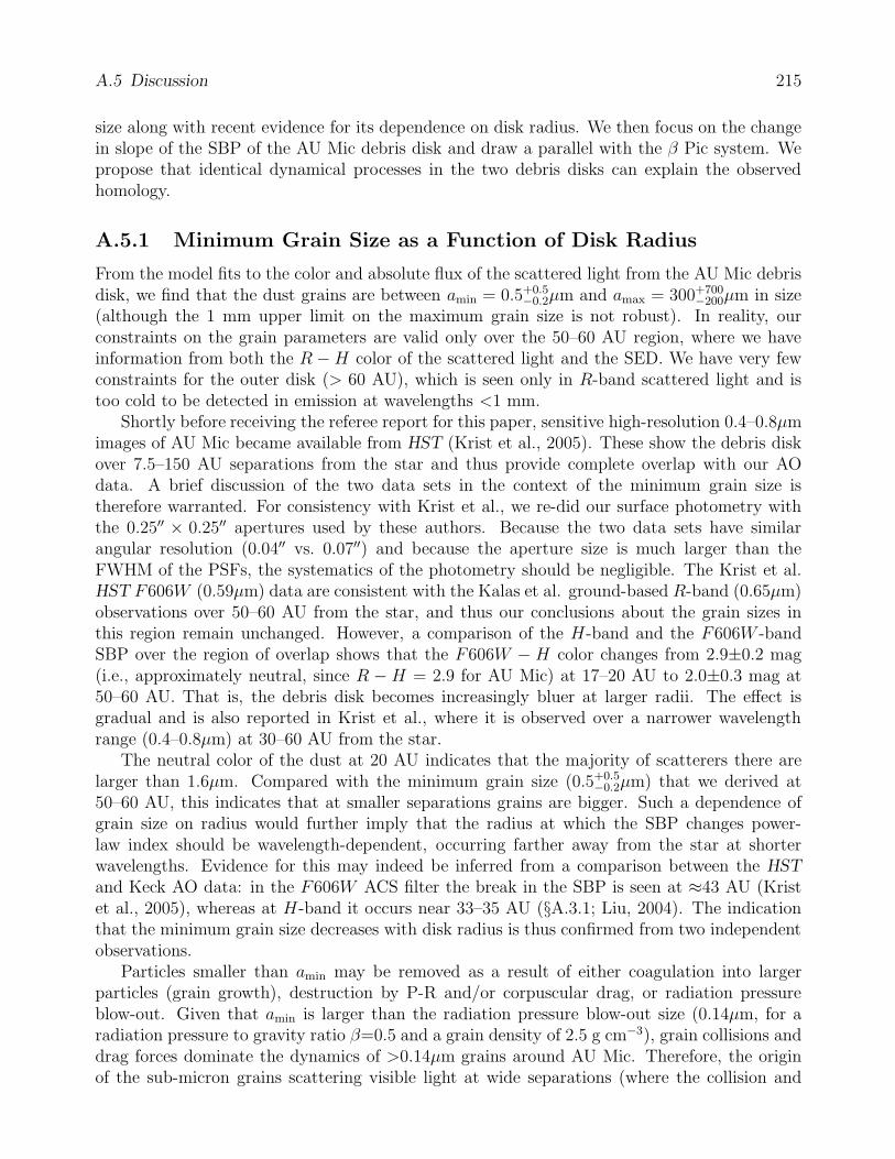
A.5 Discussion 215
size along with recent evidence for its dependence on disk radius. We then focus on the changein slope of the SBP of the AU Mic debris disk and draw a parallel with the β Pic system. Wepropose that identical dynamical processes in the two debris disks can explain the observedhomology.
A.5.1 Minimum Grain Size as a Function of Disk Radius
From the model fits to the color and absolute flux of the scattered light from the AU Mic debrisdisk, we find that the dust grains are between amin = 0.5+0.5
−0.2µm and amax = 300+700−200µm in size
(although the 1 mm upper limit on the maximum grain size is not robust). In reality, ourconstraints on the grain parameters are valid only over the 50–60 AU region, where we haveinformation from both the R −H color of the scattered light and the SED. We have very fewconstraints for the outer disk (> 60 AU), which is seen only in R-band scattered light and istoo cold to be detected in emission at wavelengths <1 mm.
Shortly before receiving the referee report for this paper, sensitive high-resolution 0.4–0.8µmimages of AU Mic became available from HST (Krist et al., 2005). These show the debris diskover 7.5–150 AU separations from the star and thus provide complete overlap with our AOdata. A brief discussion of the two data sets in the context of the minimum grain size istherefore warranted. For consistency with Krist et al., we re-did our surface photometry withthe 0.25′′ × 0.25′′ apertures used by these authors. Because the two data sets have similarangular resolution (0.04′′ vs. 0.07′′) and because the aperture size is much larger than theFWHM of the PSFs, the systematics of the photometry should be negligible. The Krist et al.HST F606W (0.59µm) data are consistent with the Kalas et al. ground-based R-band (0.65µm)observations over 50–60 AU from the star, and thus our conclusions about the grain sizes inthis region remain unchanged. However, a comparison of the H-band and the F606W -bandSBP over the region of overlap shows that the F606W − H color changes from 2.9±0.2 mag(i.e., approximately neutral, since R − H = 2.9 for AU Mic) at 17–20 AU to 2.0±0.3 mag at50–60 AU. That is, the debris disk becomes increasingly bluer at larger radii. The effect isgradual and is also reported in Krist et al., where it is observed over a narrower wavelengthrange (0.4–0.8µm) at 30–60 AU from the star.
The neutral color of the dust at 20 AU indicates that the majority of scatterers there arelarger than 1.6µm. Compared with the minimum grain size (0.5+0.5
−0.2µm) that we derived at50–60 AU, this indicates that at smaller separations grains are bigger. Such a dependence ofgrain size on radius would further imply that the radius at which the SBP changes power-law index should be wavelength-dependent, occurring farther away from the star at shorterwavelengths. Evidence for this may indeed be inferred from a comparison between the HSTand Keck AO data: in the F606W ACS filter the break in the SBP is seen at ≈43 AU (Kristet al., 2005), whereas at H-band it occurs near 33–35 AU (§A.3.1; Liu, 2004). The indicationthat the minimum grain size decreases with disk radius is thus confirmed from two independentobservations.
Particles smaller than amin may be removed as a result of either coagulation into largerparticles (grain growth), destruction by P-R and/or corpuscular drag, or radiation pressureblow-out. Given that amin is larger than the radiation pressure blow-out size (0.14µm, for aradiation pressure to gravity ratio β=0.5 and a grain density of 2.5 g cm−3), grain collisions anddrag forces dominate the dynamics of >0.14µm grains around AU Mic. Therefore, the originof the sub-micron grains scattering visible light at wide separations (where the collision and

A.5 Discussion 216
P-R time scales are longer than the age of the star) may also be primordial: rather than beingblown out from the inner disk, these grains may be remnant from the proto-stellar cloud thatnever coagulated beyond an ISM grain size distribution.
A.5.2 The Change in the SBP Power-law Index: A Comparison with
β Pic
It is not surprising that our preferred model cannot reproduce the detailed structure of our highangular resolution IR image. The model parameters were found only after a coarse sampling ofthe parameter space and through a number of simplistic assumptions that merely approximatethe physical conditions in the AU Mic debris disk. In particular, under the assumption of auniform grain size and density distribution over 10–1000 AU, the MC3D model cannot mimicthe SBP slope change at ∼33 AU and the clumpy substructure over 17–60 AU described in Liu(2004) and confirmed in §A.3.1. While the dust clumps are high-order perturbations that mayrequire dynamical considerations for proper modeling, the change in the SBP potentially couldbe explained in the framework of existing dust disk scenarios.
The occurrence of the power-law break at similar radii in the SBPs of both arms of theprojected disk suggests that this is a ring-like structure surrounding the star, rather thana discrete feature at one location in the disk. Models involving dynamical interaction withplanets have been proposed to explain ring-like structures in circumstellar disks (e.g., Roqueset al., 1994; Liou & Zook, 1999; Kenyon et al., 1999; Kenyon & Bromley, 2004), and the clumpystructure of the AU Mic disk does suggest the presence of unseen planets (Liu, 2004). However,such models tend to produce discrete rings, as around HR 4796A and HD 141569A, rather thanthe radially dimming SBP of the AU Mic disk. Similar changes in the power-law index havealso been seen in the SBPs of other resolved circumstellar disks: β Pic (Artymowicz, Paresce,& Burrows, 1990, Heap et al., 2000), TW Hya (Krist et al., 2000; Weinberger et al., 2002), andHD 100546 (Pantin, Waelkens, & Lagage, 2000; Augereau et al., 2001). A different mechanism,not necessarily involving planets, may be at play in these systems.
The TW Hya and HD 100546 circumstellar disks are gas-rich and have large mid-planeoptical depths, and hence are very much unlike the gas-poor (Roberge et al., 2004), opticallythin AU Mic debris disk. However, a comparison with β Pic is particularly illuminating becauseof the similar viewing geometry of the two systems and their identical ages. In the remainderof this section we seek a common disk architecture that can self-consistently account for thebroken power-law morphology of the SBPs of these two debris disks.
The SBP of β Pic exhibits a break at 5–6′′ (100–120 AU) from the star (e.g., Golimowski,Durrance, & Clampin, 1993, Heap et al., 2000), with similar values (from –1 to –4) of thepower-law index on either side of the break as in the SBP of AU Mic. From K ′-band (0.21µm)AO observations resolving the β Pic disk over 1.5′′–6′′, Mouillet et al. (1997) observe the breakat a somewhat smaller radius, 4–4.5′′ (75–85 AU), with a smaller change in the SBP power-lawindex (from –1 to –3). This may be the inner edge of the SBP break observed in the visible ormay indicate a wavelength-dependence of the β Pic break radius similar to the one potentiallyseen in the AU Mic disk (§A.5.1). However, because the Mouillet et al. K′-band data do notextend beyond the optical break radius (6′′) and because the change in the power-law indexobserved at K′ does not span the full range of power-law indices inferred from optical imaging,this data set will not be considered further.
Artymowicz et al. (1989) model the break in optical SBP of the β Pic disk using two different

A.5 Discussion 217
power laws for the number density of dust particles in the disk for radii less than or greaterthan 100 AU, respectively. Backman et al. (1992) consider the possibility of differing grainsizes, in addition. While either model may correctly describe the architecture of the β Pic disk,both are purely phenomenological, as they do not model the physics behind the discontinuityin the disk. Based on the apparent homology between these two debris disks, we believe thata plausible two-component model should be able to explain both systems self-consistently. Inlight of this, several physical scenarios from the subsequent literature are considered below. Wefind that none of them offer a unique explanation and propose separate hypotheses in §A.5.2.3and A.5.2.4.
A.5.2.1 Ice or Comet Evaporation
Backman et al. (1992) and Pantin, Lagage, & Artymowicz (1997) suggest that the discontinuityin the SBP of β Pic may correspond to the location of the “ice boundary” in the disk: alldust particles at separations >100 AU are covered with ice, while at shorter separations somemay not be. This results in a deficiency of highly reflective particles in the inner regions,creating a shallower power-law index for the scattered light profile. In an optically thin diskthe radius of the ice boundary should scale as the square root of the stellar luminosity. AdoptingLAUMic = 0.13L (Table A.1) and LβPic = 8.7L, and assuming identical grain chemistry inthe two systems, we find that the corresponding boundary around AU Mic should scale downto a radius of 13–15 AU, too close to account for the break at 33 AU.
An alternative hypothesis, involving dust extraction through evaporation of gas from areservoir of cometary bodies around β Pic, is proposed by Lecavelier des Etangs, Vidal-Madjar,& Ferlet (1996). However, the radial distance of this evaporating reservoir should scale in thesame manner as that of the ice boundary. Hence, neither of these two hypotheses can be appliedsimultaneously to AU Mic and β Pic.
A.5.2.2 A Belt of Parent Bodies
A reservoir of parent bodies at a discrete range of separations from AU Mic could explainthe kink in the SBP. Gorkavyi et al. (1997) calculate that the Main asteroid belt in the SolarSystem should produce a break in the power-law index of the number density distribution ofinterplanetary grains from −1.3 to −6.4 at 0.5–3.0 AU from the Sun. These predictions areconsistent with empirical data from radar meteors and from impact detectors on spacecraft(Divine, 1993). The inner edge of this belt of asteroids in the AU Mic and β Pic systems wouldbe at the location of the kinks, at ∼33 AU and ∼110 AU from the stars, respectively. Bycontinuing the analogy with the Solar System, such belts of parent bodies would likely needto be maintained in a discrete range of orbits through mean motion resonances with planets(e.g., Liou & Zook, 1997, and references therein). That is, this particular scenario may providefurther indication for the existence of planets in the two disks, in addition to the evidencearising from the their clumpy structure. However, this model is poorly constrained, as we arefree to invoke a belt of parent bodies at any distance from either star.
A.5.2.3 Collisional Evolution
For two stars of the same age, the disk around the more massive star is expected to be colli-sionally evolved out to a greater radius because of the inverse scaling of the orbital period (and
A.5 Discussion 218
hence, collision frequency) with orbital radius and stellar mass. The collisional time scale forparticles of mean size a on a circular orbit of radius r from a star of mass M∗ is
tcoll ∼P
4π2a2rn(r)∝ r1/2
M1/2∗ n0r−γ
=rγ+1/2
M1/2∗ n0
, (A.1)
where P is the orbital period, and n0 is the normalization constant for the number densitydistribution, which we presume scales as Mdust. Given the approximate ratios of the stellarmasses of AU Mic and β Pic (0.28, assuming Mβ Pic = 1.8M), and of their circumstellar dustmasses, (0.2 ± 0.1, where the mass of the β Pic disk was taken as the average of the estimatesfrom Sheret, Dent, & Wyatt (2004) and Dent et al. (2000)) and assuming 33 AU and 110 AUas the radii of the kinks in the corresponding SBPs, we find that for γ = 1.5+0.3
−0.4 the collisionaltime scales at the respective separations around the two stars are equal. This would implySBPs decreasing approximately as r−γ−1 = r−2.5, which is within the ranges found in §A.3.1for AU Mic and in Heap et al. (2000) for β Pic, and agrees with the fit to the mean AU MicH-band SBP (power-law index of −2.3 ± 0.2; Figure A.4). Therefore, in this scenario the twodisk systems scale correctly within the errors, indicating that whatever process we are observingmay scale with the mean time between inter-particle collisions. Although the collisional time-scale at the location of the break in the AU Mic SBP is considerably shorter (1–3 Myr) thanthe age of the star (8–20 Myr), other, slower processes in the disk, e.g., grain growth, may scalelinearly with the time between particle collisions. As noted in §A.5.1, grain growth could alsoexplain the observed dependence of grain size with orbital radius.
A.5.2.4 Poynting-Robertson Drag
The observed change in the power-law index of the SBP may be a reflection of the finite lifetimesof sub-micron grains in the inner disk. Having ruled out radiation pressure as a dominant forceon grains larger than 0.14µm (§A.5.1), we propose a hypothesis based on drag forces for grainremoval, in particular P-R drag. Although corpuscular drag may dominate the dynamics ofdust around M stars (e.g., Fleming, Schmitt, & Giampapa, 1995), the strength of stellar windsfrom M dwarfs remains largely unknown. We therefore ignore corpuscular drag in the followinganalysis (see Plavchan, Jura, & Lipscy, 2005, for a discussion of the role of corpuscular drag inthe AU Mic disk) and consider only P-R drag. As long as the magnitude of the corpusculardrag force around AU Mic is not much greater than the magnitude of the P-R drag force, theconclusions remain unchanged.
If P-R drag was responsible for the depletion of micron-sized grains in the inner disks ofAU Mic and β Pic, then the P-R lifetime (tPR) of the smallest grains amin should be constantas a function of disk radius r and should equal the age of the stars (tage). This can be inferredfrom the expression for the P-R lifetime of a particle of size a (see, e.g., Burns, Lamy, & Soter,1979):
tPR(a, r) =
(
4πaρ
3
)(
c2r2
L∗
)
, (A.2)
where ρ is the mean grain density (2.5 g cm−3 for silicates), and c is the speed of light. Basedon the assumption that P-R drag is the dominant removal mechanism for grains larger than theblow-out size (0.14µm), the P-R lifetime of the smallest grains is tPR(amin, r) = tage = const.Note, however, that the size of the smallest grains, amin, is not a constant, but varies as
A.6 Conclusion 219
amin ∝ r−2.For AU Mic we found amin ≥ 0.3µm at 50–60 AU and amin ≥ 1.6µm at 17–20 AU (§A.5.1).
We obtain tPR(0.3µm, 50AU) = 9.9 Myr and tPR(1.6µm, 20AU) = 8.4 Myr. We do not haveinformation about the change in amin as a function of radius in β Pic. We only note that frommid-IR and visual images, Artymowicz et al. (1989) find that they require “few-micron-sized”silicate grains2 to model the scattered light at >6.0′′ (>115 AU) from the star. Assuming aminimum grain size of 3µm, we find tPR(3µm, 115AU) = 7.8 Myr around β Pic. Given theuncertainty in amin, the obtained P-R time-scales are not constrained to better than a factor of1.5–2. Nevertheless, they are remarkably similar and agree well with the ages of AU Mic andβ Pic.
A.5.2.5 Summary of Proposed Scenarios
We find that dynamical scenarios based on collisional evolution or P-R drag in debris disks offersimpler and more self-consistent accounts of the homology between the SBPs of the AU Mic andβ Pic debris disks, compared to scenarios relying on ice/grain evaporation or belts of orbitingparent bodies. Moreover, both our hypotheses can account for the inferred decrease in theminimum grain size with increasing separation from AU Mic. We therefore conclude that bothare plausible. Given the similarities in their predictions, we do not single out which one ofthem is more likely, but defer that analysis to a more detailed theoretical work. Regardless ofwhich of the two processes is found to be dominant, we can confidently claim that opticallythin circumstellar disks exhibiting breaks in their SBPs are observed in transition between aprimordial and a debris state.
A.6 Conclusion
We have used AO H-band observations of scattered light to probe the morphology of the debrisdisk at 17–60 AU from the young nearby M dwarf AU Mic. We find that the disk is within∼1 of edge-on and that it exhibits a number of morphological peculiarities: radial asymmetry,spatially resolved clumps, and a change in the power-law index of the surface brightness profilenear 33 AU. The observed morphology agrees with that reported in Liu (2004) and is suggestiveof the existence of planetary perturbers in the disk. No planets are detected down to 1MJup at>20 AU.
We use a Monte Carlo three-dimensional dust disk model to constrain the overall diskparameters by optimizing them against the AU Mic SED and near-IR and optical scatteredlight images of the disk (this paper; Kalas et al., 2004). The combined use of SED data tracingthe thermal emission from large grains and of imaging data tracing grain properties allows us tobreak several important degeneracies in models of circumstellar disks that cannot be resolvedusing only one of the two data sets. From the SED we confirm the previously inferred (Liuet al., 2004) circumstellar dust mass of 0.011M⊕, and from the properties of the scattered lightwe infer that the debris particles are ≥ 0.5+0.5
−0.2µm in size at 50–60 AU from AU Mic. Wefind tentative evidence for a maximum grain size of 300+500
−200µm. However, since the data arenot sensitive to particles 1 mm, the result is consistent with no upper limit on the grain
2A second solution involving 1–15µm ice grains is found to be equally plausible. However, its grain propertiesdiffer widely from the ones adopted for the AU Mic circumstellar dust in this paper.

A.6 Conclusion 220
size. Assuming a single dust size and density distribution, we estimate that the radius of theinner disk clearing is 10 AU. However, smaller (∼1 AU) gap sizes cannot be ruled out if ashallower density profile (as observed inwards of 33 AU) and/or larger grains in the inner disk(as evidenced from the optical-near-IR color of the disk) are adopted. We attribute the lack ofsub-micron particles in the inner disk to grain growth, destruction by P-R and/or corpusculardrag (for grains >0.14µm), or to blow-out by radiation pressure (for grains <0.14µm). All ofthese mechanisms can explain the increase in relative density of small grains with increasingradius in the disk.
The MC3D model can account for the overall disk profile and colors to first order, al-though our one-component model fails to reproduce higher-order effects, such as the change inpower-law index of the SBP. We have discussed a number of scenarios that may be capable ofreproducing such a change in the joint context of the AU Mic and β Pic debris disks. We findthat models dividing the disk into two separate components, with different grain distributionand/or composition, represent the combined SED and imaging data best. In particular, classesof models that scale with the collision or the P-R time-scale are most likely to explain bothdebris disks self-consistently.
Future high-dynamic range imaging observations probing closer to AU Mic (e.g., with nullinginterferometry in the mid-IR) will further narrow down the architecture of its debris disk.Photometric and spectroscopic observations with Spitzer could better constrain the SED ofAU Mic and could be used to look for spectroscopic features. These could trace small amountsof dust and gas in the inner disk, even if no continuum excess is seen at < 25µm.

Bibliography
Abt, H. A., & Levy, S. G. 1976, ApJS, 30, 273
Ackerman, A. S., & Marley, M. S. 2001, ApJ, 556, 872
Adams, J. D., Stauffer, J. R., Monet, D. G., Skrutskie, M. F., & Beichman, C. A. 2001, AJ,121, 2053
Ali, B., Carr, J. S., Depoy, D. L., Frogel, J. A., & Sellgren, K. 1995, AJ, 110, 2415
Allende Prieto, C., & Lambert, D. L. 1999, A&A, 352, 555
Andersen, J. 1991, A&A Rev., 3, 91
Apai, D., Pascucci, I., Brandner, W., Henning, T., Lenzen, R., Potter, D. E., Lagrange, A.-M.,& Rousset, G. 2004, A&A, 415, 671
Appenzeller, I., Thiering, I., Zickgraf, F.-J., Krautter, J., Voges, W., Chavarria, C., Kneer, R.,Mujica, R., Pakull, M., Rosso, C., Ruzicka, F., Serrano, A., & Ziegler, B. 1998, ApJS, 117,319
Artymowicz, P., Burrows, C., & Paresce, F. 1989, ApJ, 337, 494
Artymowicz, P., Paresce, F., & Burrows, C. 1990, Advances in Space Research, 10, 81
Augereau, J. C., Lagrange, A. M., Mouillet, D., & Menard, F. 2001, A&A, 365, 78
Augereau, J. C., & Papaloizou, J. C. B. 2004, A&A, 414, 1153
Aumann, H. H., Beichman, C. A., Gillett, F. C., de Jong, T., Houck, J. R., Low, F. J.,Neugebauer, G., Walker, R. G., & Wesselius, P. R. 1984, ApJ, 278, L23
Backman, D., & Gillett, F. C. 1987, Lecture Notes in Physics, Berlin Springer Verlag, 291, 340
Backman, D. E., & Paresce, F. 1993, in Protostars and Planets III, 1253–1304
Backman, D. E., Witteborn, F. C., & Gillett, F. C. 1992, ApJ, 385, 670
Bahcall, J. N., & Soneira, R. M. 1980, ApJS, 44, 73
Baraffe, I., Chabrier, G., Allard, F., & Hauschildt, P. H. 1995, ApJ, 446, L35+
—. 1998, A&A, 337, 403
221
BIBLIOGRAPHY 222
Baraffe, I., Chabrier, G., Barman, T. S., Allard, F., & Hauschildt, P. H. 2003, A&A, 402, 701
Barrado y Navascues, D. 1998, A&A, 339, 831
Barrado y Navascues, D., Stauffer, J. R., Song, I., & Caillault, J.-P. 1999, ApJ, 520, L123
Basri, G., Marcy, G. W., & Graham, J. R. 1996, ApJ, 458, 600
Bate, M. R., Bonnell, I. A., & Bromm, V. 2002, MNRAS, 332, L65
—. 2003, MNRAS, 339, 577
Bayes, T. 1763, Philosophical Transactions of the Royal Society of London, 53, 370, can alsobe found at: http://www.stat.ucla.edu/history/essay.pdf
Bertin, E., & Arnouts, S. 1996, A&AS, 117, 393
Bessell, M. S. 1991, AJ, 101, 662
Bessell, M. S., & Brett, J. M. 1988, PASP, 100, 1134
Beust, H., Lagrange-Henri, A. M., Vidal-Madjar, A., & Ferlet, R. 1989, A&A, 223, 304
Beust, H., Vidal-Madjar, A., Ferlet, R., & Lagrange-Henri, A. M. 1990, A&A, 236, 202
Beuzit, J.-L., Segransan, D., Forveille, T., Udry, S., Delfosse, X., Mayor, M., Perrier, C.,Hainaut, M.-C., Roddier, C., Roddier, F., & Martın, E. L. 2004, A&A, 425, 997
Bloemhof, E. E. 2003, ApJ, 582, L59
Bloemhof, E. E., Marsh, K. A., Dekany, R. G., Troy, M., Marshall, J., Oppenheimer, B. R.,Hayward, T. L., & Brandl, B. 2000, in Proc. SPIE Vol. 4007, Adaptive Optical SystemsTechnology, Peter L. Wizinowich; Ed., 889–898
Boccaletti, A., Riaud, P., & Rouan, D. 2002, PASP, 114, 132
Bodenheimer, P. 1965, ApJ, 142, 451
Bodenheimer, P., Tohline, J. E., & Black, D. C. 1980, ApJ, 242, 209
Bohren, C. F., & Huffman, D. R. 1983, Absorption and scattering of light by small particles(New York: Wiley, 1983)
Boss, A. P. 2002, ApJ, 576, 462
Bouvier, J., Rigaut, F., & Nadeau, D. 1997, A&A, 323, 139
Bouy, H., Brandner, W., Martın, E. L., Delfosse, X., Allard, F., & Basri, G. 2003, AJ, 126,1526
Bouy, H., Duchene, G., Kohler, R., Brandner, W., Bouvier, J., Martın, E. L., Ghez, A., Delfosse,X., Forveille, T., Allard, F., Baraffe, I., Basri, G., Close, L., & McCabe, C. E. 2004, A&A,423, 341

BIBLIOGRAPHY 223
Brandner, W., Zinnecker, H., Alcala, J. M., Allard, F., Covino, E., Frink, S., Kohler, R.,Kunkel, M., Moneti, A., & Schweitzer, A. 2000, AJ, 120, 950
Breger, M. 1986, ApJ, 309, 311
Briceno, C., Luhman, K. L., Hartmann, L., Stauffer, J. R., & Kirkpatrick, J. D. 2002, ApJ,580, 317
Briggs, R. E. 1962, AJ, 67, 710
Brown, R. A. 2004, ApJ, 607, 1003
—. 2005, ApJ, 624, 1010
Burgasser, A. J., Kirkpatrick, J. D., Brown, M. E., Reid, I. N., Burrows, A., Liebert, J.,Matthews, K., Gizis, J. E., Dahn, C. C., Monet, D. G., Cutri, R. M., & Skrutskie, M. F.2002, ApJ, 564, 421
Burgasser, A. J., Kirkpatrick, J. D., Reid, I. N., Brown, M. E., Miskey, C. L., & Gizis, J. E.2003, ApJ, 586, 512
Burns, J. A., Lamy, P. L., & Soter, S. 1979, Icarus, 40, 1
Burrows, A., Hubbard, W. B., Lunine, J. I., & Liebert, J. 2001, Reviews of Modern Physics,73, 719
Burrows, A., & Liebert, J. 1993, Reviews of Modern Physics, 65, 301
Burrows, A., Marley, M., Hubbard, W. B., Lunine, J. I., Guillot, T., Saumon, D., Freedman,R., Sudarsky, D., & Sharp, C. 1997, ApJ, 491, 856
Buscombe, W. 1998, VizieR Online Data Catalog, 3206, 0
Buscombe, W., & Foster, B. E. 1997, VizieR Online Data Catalog, 3189, 0
Campbell, B., Walker, G. A. H., & Yang, S. 1988, ApJ, 331, 902
Cannon, A. J., & Pickering, E. C. 1901, Ann. Astron. Obs. Harvard Coll., 131, 28(II)
Cardelli, J. A., Clayton, G. C., & Mathis, J. S. 1989, ApJ, 345, 245
Carpenter, J. M. 2001, AJ, 121, 2851
Carpenter, J. M., & Stauffer, J. 2003, fEPS internal report
Carpenter, J. M., Wolf, S., Schreyer, K., Launhardt, R., & Henning, T. 2004, ArXiv Astro-physics e-prints
Carson, J., Eikenberry, S., Brandl, B., Wilson, J. C., & Hayward, T. L. 2003, in IAU Sympo-sium, 271
Carson, J. C., Eikenberry, S. S., Brandl, B. R., Wilson, J. C., & Hayward, T. L. 2004, AmericanAstronomical Society Meeting Abstracts, 205, 0
BIBLIOGRAPHY 224
—. 2005, ArXiv Astrophysics e-prints:astro-ph/0506287
Carter, B. D., Butler, R. P., Tinney, C. G., Jones, H. R. A., Marcy, G. W., McCarthy, C.,Fischer, D. A., & Penny, A. J. 2003, ApJ, 593, L43
Cashwell, E. D., & Everett, C. J. 1959, A Practical Manual on the Monte Carlo Method forRandom Walk Problems (New York: Pergamon Press, 1959)
Chabrier, G., & Baraffe, I. 1997, A&A, 327, 1039
—. 2000, ARA&A, 38, 337
Chabrier, G., Baraffe, I., Allard, F., & Hauschildt, P. 2000, ApJ, 542, 464
Chauvin, G., Lagrange, A.-M., Dumas, C., Zuckerman, B., Mouillet, D., Song, I., Beuzit, J.-L.,& Lowrance, P. 2004, A&A, 425, L29
—. 2005a, A&A, 438, L25
Chauvin, G., Lagrange, A.-M., Zuckerman, B., Dumas, C., Mouillet, D., Song, I., Beuzit, J.-L.,Lowrance, P., & Bessell, M. S. 2005b, A&A, 438, L29
Chauvin, G., Thomson, M., Dumas, C., Beuzit, J.-L., Lowrance, P., Fusco, T., Lagrange, A.-M.,Zuckerman, B., & Mouillet, D. 2003, A&A, 404, 157
Ciardi, D. R., van Belle, G. T., Akeson, R. L., Thompson, R. R., Lada, E. A., & Howell, S. B.2001, ApJ, 559, 1147
Clampin, M., Krist, J. E., Ardila, D. R., Golimowski, D. A., Hartig, G. F., Ford, H. C.,Illingworth, G. D., Bartko, F., Benıtez, N., Blakeslee, J. P., Bouwens, R. J., Broadhurst,T. J., Brown, R. A., Burrows, C. J., Cheng, E. S., Cross, N. J. G., Feldman, P. D., Franx,M., Gronwall, C., Infante, L., Kimble, R. A., Lesser, M. P., Martel, A. R., Menanteau, F.,Meurer, G. R., Miley, G. K., Postman, M., Rosati, P., Sirianni, M., Sparks, W. B., Tran,H. D., Tsvetanov, Z. I., White, R. L., & Zheng, W. 2003, AJ, 126, 385
Close, L. M., Lenzen, R., Guirado, J. C., Nielsen, E. L., Mamajek, E. E., Brandner, W.,Hartung, M., Lidman, C., & Biller, B. 2005, Nature, 433, 286
Close, L. M., Siegler, N., Freed, M., & Biller, B. 2003, ApJ, 587, 407
Close, L. M. e. a. 2004, in ESO Workshop on Adaptive Optics, ASP, in press,http://exoplanet.as.arizona.edu/ lclose/talks/ins/close1.ps
Cooper, C. S., Sudarsky, D., Milsom, J. A., Lunine, J. I., & Burrows, A. 2003, ApJ, 586, 1320
Couteau, P. 1960, Journal des Observateurs, 43, 41
Cox, A. N. 2000, Allen’s astrophysical quantities (4th ed. Publisher: New York: AIP Press;Springer, 2000. Edited by Arthur N. Cox. ISBN: 0387987460)
Crawford, D. L., & Perry, C. L. 1976, AJ, 81, 419
BIBLIOGRAPHY 225
Cutri, R. M., Skrutskie, M. F., van Dyk, S., Beichman, C. A., Carpenter, J. M., Chester, T.,Cambresy, L., Evans, T., Fowler, J., Gizis, J., Howard, E., Huchra, J., Jarrett, T., Kopan,E. L., Kirkpatrick, J. D., Light, R. M., Marsh, K. A., McCallon, H., Schneider, S., Stiening,R., Sykes, M., Weinberg, M., Wheaton, W. A., Wheelock, S., & Zacarias, N. 2003, VizieROnline Data Catalog, 2246, 0
Dahn, C. C., Harris, H. C., Vrba, F. J., Guetter, H. H., Canzian, B., Henden, A. A., Levine,S. E., Luginbuhl, C. B., Monet, A. K. B., Monet, D. G., Pier, J. R., Stone, R. C., Walker,R. L., Burgasser, A. J., Gizis, J. E., Kirkpatrick, J. D., Liebert, J., & Reid, I. N. 2002, AJ,124, 1170
Dannerbauer, H., Lehnert, M. D., Lutz, D., Tacconi, L., Bertoldi, F., Carilli, C., Genzel, R., &Menten, K. 2002, ApJ, 573, 473
D’Antona, F., & Mazzitelli, I. 1997, Memorie della Societa Astronomica Italiana, 68, 807
de La Reza, R., Torres, C. A. O., Quast, G., Castilho, B. V., & Vieira, G. L. 1989, ApJ, 343,L61+
de Zeeuw, P. T., Hoogerwerf, R., de Bruijne, J. H. J., Brown, A. G. A., & Blaauw, A. 1999,AJ, 117, 354
Decin, G., Dominik, C., Waters, L. B. F. M., & Waelkens, C. 2003, ApJ, 598, 636
Delfosse, X., Forveille, T., Segransan, D., Beuzit, J.-L., Udry, S., Perrier, C., & Mayor, M.2000, A&A, 364, 217
Dent, W. R. F., Walker, H. J., Holland, W. S., & Greaves, J. S. 2000, MNRAS, 314, 702
Devillard, N. 2001, in ASP Conf. Ser. 238: Astronomical Data Analysis Software and SystemsX, 525–+
Diolaiti, E., Bendinelli, O., Bonaccini, D., Close, L., Currie, D., & Parmeggiani, G. 2000,A&AS, 147, 335
Divine, N. 1993, J. Geophys. Res., 98, 17029
Donahue, R. A. 1993, Ph.D. Thesis, New Mexico State University, University Park, New Mexico
Donahue, R. A. 1998, in ASP Conf. Ser. 154: Cool Stars, Stellar Systems, and the Sun, 1235–+
Donnison, J. R., & Mikulskis, D. F. 1995, MNRAS, 272, 1
Dorren, J. D., & Guinan, E. F. 1994, ApJ, 428, 805
Draine, B. T., & Lee, H. M. 1984, ApJ, 285, 89
Draine, B. T., & Malhotra, S. 1993, ApJ, 414, 632
Drilling, J. S., & Landolt, A. U. 2000, in Allen’s Astrophysical Quantities, ed. A. Cox, 4th edn.(New York: Springer), 382

BIBLIOGRAPHY 226
Duncan, D. K. 1981, ApJ, 248, 651
Duncan, D. K., & Jones, B. F. 1983, ApJ, 271, 663
Duquennoy, A., & Mayor, M. 1991, A&A, 248, 485
Eggen, O. J. 1965, ARA&A, 3, 235
—. 1996, AJ, 111, 466
Els, S. G., Sterzik, M. F., Marchis, F., Pantin, E., Endl, M., & Kurster, M. 2001, A&A, 370,L1
Endl, M., Hatzes, A. P., Cochran, W. D., McArthur, B., Allende Prieto, C., Paulson, D. B.,Guenther, E., & Bedalov, A. 2004, ApJ, 611, 1121
EROS Collaboration, Goldman, B., Delfosse, X., Forveille, T., Afonso, C., Alard, C., Albert,J. N., Andersen, J., Ansari, R., Aubourg, E., Bareyre, P., Bauer, F., Beaulieu, J. P., Borsen-berger, J., Bouquet, A., Char, S., Charlot, X., Couchot, F., Coutures, C., Derue, F., Ferlet,R., Fouque, P., Glicenstein, J. F., Gould, A., Graff, D., Gros, M., Haissinski, J., Hamilton,J. C., Hardin, D., de Kat, J., Kim, A., Lasserre, T., Lesquoy, E., Loup, C., Magneville,C., Mansoux, B., Marquette, J. B., Martın, E. L., Maurice, E., Milsztajn, A., Moniez, M.,Palanque-Delabrouille, N., Perdereau, O., Prevot, L., Regnault, N., Rich, J., Spiro, M.,Vidal-Madjar, A., Vigroux, L., & Zylberajch, S. 1999, A&A, 351, L5
Fabricius, C., & Makarov, V. V. 2000, A&A, 356, 141
Farihi, J., Becklin, E. E., & Zuckerman, B. 2005, ArXiv Astrophysics e-prints:astro-ph/0506017
Fischer, D. A. 1998, Ph.D. Thesis, University of California, Santa Cruz, California
Fischer, D. A., & Marcy, G. W. 1992, ApJ, 396, 178
Fischer, D. A., Marcy, G. W., Butler, R. P., Vogt, S. S., Walp, B., & Apps, K. 2002, PASP,114, 529
Fleming, T. A. 1998, ApJ, 504, 461
Fleming, T. A., Schmitt, J. H. M. M., & Giampapa, M. S. 1995, ApJ, 450, 401
Freeman, P. E., Kashyap, V., Rosner, R., & Lamb, D. Q. 2002, ApJS, 138, 185
Frink, S., Roser, S., Neuhauser, R., & Sterzik, M. F. 1997, A&A, 325, 613
Gaidos, E. J. 1998, PASP, 110, 1259
Gatewood, G., & de Jonge, J. K. 1995, ApJ, 450, 364
Geballe, T. R., Knapp, G. R., Leggett, S. K., Fan, X., Golimowski, D. A., Anderson, S.,Brinkmann, J., Csabai, I., Gunn, J. E., Hawley, S. L., Hennessy, G., Henry, T. J., Hill,G. J., Hindsley, R. B., Ivezic, Z., Lupton, R. H., McDaniel, A., Munn, J. A., Narayanan,V. K., Peng, E., Pier, J. R., Rockosi, C. M., Schneider, D. P., Smith, J. A., Strauss, M. A.,Tsvetanov, Z. I., Uomoto, A., York, D. G., & Zheng, W. 2002, ApJ, 564, 466
BIBLIOGRAPHY 227
Gelino, C. R., Kirkpatrick, J. D., & Burgasser, A. J. 2004, American Astronomical SocietyMeeting Abstracts, 205, 0
Ghez, A. M., McCarthy, D. W., Patience, J. L., & Beck, T. L. 1997, ApJ, 481, 378
Ghez, A. M., Neugebauer, G., & Matthews, K. 1993, AJ, 106, 2005
Gizis, J. E., Kirkpatrick, J. D., Burgasser, A., Reid, I. N., Monet, D. G., Liebert, J., & Wilson,J. C. 2001, ApJ, 551, L163
Gizis, J. E., Reid, I. N., & Hawley, S. L. 2002, AJ, 123, 3356
Gliese, W., & Jahreiß, H. 1991, Preliminary Version of the Third Catalogue of Nearby Stars,Tech. rep., Astronomisches Rechen-Institut, Heidelberg, Germany
Goldader, J. D., Meurer, G., Heckman, T. M., Seibert, M., Sanders, D. B., Calzetti, D., &Steidel, C. C. 2002, ApJ, 568, 651
Golimowski, D. A., Durrance, S. T., & Clampin, M. 1993, ApJ, 411, L41
Golimowski, D. A., Leggett, S. K., Marley, M. S., Fan, X., Geballe, T. R., Knapp, G. R., Vrba,F. J., Henden, A. A., Luginbuhl, C. B., Guetter, H. H., Munn, J. A., Canzian, B., Zheng, W.,Tsvetanov, Z. I., Chiu, K., Glazebrook, K., Hoversten, E. A., Schneider, D. P., & Brinkmann,J. 2004, AJ, 127, 3516
Gorkavyi, N. N., Ozernoy, L. M., Mather, J. C., & Taidakova, T. 1997, ApJ, 488, 268
Gorkavyi, N. N., & Taidakova, T. A. 2001, Bulletin of the American Astronomical Society, 33,1431
Gorlova, N., Padgett, D. L., Rieke, G. H., Muzerolle, J., Morrison, J. E., Gordon, K. D.,Engelbracht, C. W., Hines, D. C., Hinz, J. C., Noriega-Crespo, A., Rebull, L., Stansberry,J. A., Stapelfeldt, K. R., Su, K. Y. L., & Young, E. T. 2004, ApJS, 154, 448
Gorlova, N. I., Meyer, M. R., Rieke, G. H., & Liebert, J. 2003, ApJ, 593, 1074
Gray, R. O. 1992, A&A, 265, 704
Greaves, J. S., Holland, W. S., Moriarty-Schieven, G., Jenness, T., Dent, W. R. F., Zuckerman,B., McCarthy, C., Webb, R. A., Butner, H. M., Gear, W. K., & Walker, H. J. 1998, ApJ,506, L133
Green, P. J., Ali, B., & Napiwotzki, R. 2000, ApJ, 540, 992
Gulliver, A. F., Hill, G., & Adelman, S. J. 1994, ApJ, 429, L81
Habing, H. J., Dominik, C., Jourdain de Muizon, M., Laureijs, R. J., Kessler, M. F., Leech, K.,Metcalfe, L., Salama, A., Siebenmorgen, R., Trams, N., & Bouchet, P. 2001, A&A, 365, 545
Hale, A. 1994, AJ, 107, 306
Harper, D. A., Loewenstein, R. F., & Davidson, J. A. 1984, ApJ, 285, 808

BIBLIOGRAPHY 228
Hartkopf, W. I., & Mason, B. D. 2000, in IAU Commission on Double Stars, 1–2
Hartkopf, W. I., & Mason, B. D. 2003, http://ad.usno.navy.mil/wds/orb6/orb6c.html
—. 2005, http://ad.usno.navy.mil/wds/orb6.html
Hartkopf, W. I., Mason, B. D., & McAlister, H. A. 1996, AJ, 111, 370
Hartkopf, W. I., Mason, B. D., & Worley, C. E. 2001, AJ, 122, 3472
Harvey, P. M., Wilking, B. A., & Joy, M. 1984, Nature, 307, 441
Hauschildt, P. H., Allard, F., & Baron, E. 1999, ApJ, 512, 377
Hayashi, C., & Nakano, T. 1963, Prog. Theo. Physics, 30, 4
Hayward, T. L., Brandl, B., Pirger, B., Blacken, C., Gull, G. E., Schoenwald, J., & Houck,J. R. 2001, PASP, 113, 105
Heap, S. R., Lindler, D. J., Lanz, T. M., Cornett, R. H., Hubeny, I., Maran, S. P., & Woodgate,B. 2000, ApJ, 539, 435
Heckmann, O., Dieckvoss, W., & Kox, H. 1956, Astronomische Nachrichten, 283, 109
Heinrichsen, I., Walker, H. J., & Klaas, U. 1998, MNRAS, 293, L78
Heintz, W. D. 1978, Geophysics and Astrophysics Monographs, 15
Henry, T. J., Soderblom, D. R., Donahue, R. A., & Baliunas, S. L. 1996, AJ, 111, 439
Herbig, G. H. 1965, ApJ, 141, 588
Hertzspring, E. 1947, Annalen van de Sterrewacht te Leiden, 19, 1
Hillenbrand, L. A., Mamajek, E. E., Stauffer, J. R., Soderblom, D. R., & Meyer, M. R. 2005,ApJ, submitted
Hillenbrand, L. A., & White, R. J. 2004, ApJ, 604, 741
Hines, D., Carpenter, J. M., Bouwman, J., Kim, J. S., Silverstone, M. D., Pascucci, I., Meyer,M. R., Cohen, M., Stauffer, J. R., Stobie, B., & Watson, D. M. 2005, FEPS Data ExplanatorySupplement, v. 2.0, Tech. rep., Spitzer Science Center, California Institute of Technol-ogy, http://data.spitzer.caltech.edu/popular/feps/20050608 enhanced v1/Documents/FEPS Data Explan Supp v2.pdf
Høg, E., Fabricius, C., Makarov, V. V., Urban, S., Corbin, T., Wycoff, G., Bastian, U., Schwek-endiek, P., & Wicenec, A. 2000, A&A, 355, L27
Holland, W. S., Greaves, J. S., Dent, W. R. F., Wyatt, M. C., Zuckerman, B., Webb, R. A.,McCarthy, C., Coulson, I. M., Robson, E. I., & Gear, W. K. 2003, ApJ, 582, 1141
Holland, W. S., Greaves, J. S., Zuckerman, B., Webb, R. A., McCarthy, C., Coulson, I. M.,Walther, D. M., Dent, W. R. F., Gear, W. K., & Robson, I. 1998, Nature, 392, 788

BIBLIOGRAPHY 229
Hollenbach, D., Gorti, U., Meyer, M., Kim, J. S., Morris, P., Najita, J., Pascucci, I., Carpenter,J., Rodmann, J., Brooke, T., Hillenbrand, L., Mamajek, E., Padgett, D., Soderblom, D.,Wolf, S., & Lunine, J. 2005, ArXiv Astrophysics e-prints:astro-ph/0506252
Houdashelt, M. L., Bell, R. A., & Sweigart, A. V. 2000, AJ, 119, 1448
Jayawardhana, R., & Brandeker, A. 2001, ApJ, 561, L111
Jefferies, S. M., & Christou, J. C. 1993, ApJ, 415, 862
Jeffries, R. D. 1995, MNRAS, 273, 559
Johnson, D. R. H., & Soderblom, D. R. 1987, AJ, 93, 864
Johnson, H. L., & Mitchell, R. I. 1958, ApJ, 128, 31
Jones, H. R. A., Paul Butler, R., Tinney, C. G., Marcy, G. W., Penny, A. J., McCarthy, C.,Carter, B. D., & Pourbaix, D. 2002, MNRAS, 333, 871
Konig, B., Guenther, E. W., Woitas, J., & Hatzes, A. P. 2005, A&A, 435, 215
Kalas, P., Deltorn, J., & Larwood, J. 2001, ApJ, 553, 410
Kalas, P., Graham, J. R., & Clampin, M. 2005, Nature, 435, 1067
Kalas, P., & Jewitt, D. 1996, AJ, 111, 1347
Kalas, P., Larwood, J., Smith, B. A., & Schultz, A. 2000, ApJ, 530, L133
Kalas, P., Liu, M. C., & Matthews, B. C. 2004, Science, 303, 1990
Kasdin, N. J., Vanderbei, R. J., Spergel, D. N., & Littman, M. G. 2003, ApJ, 582, 1147
Kastner, J. H., Zuckerman, B., Weintraub, D. A., & Forveille, T. 1997, Science, 277, 67
Keenan, P. C. 1983, Bulletin d’Information du Centre de Donnees Stellaires, 24, 19
Kendall, M., & Stuart, A. 1977, The advanced theory of statistics. Vol.1: Distribution theory(London: Griffin, 1977, 4th ed.)
Kenyon, S. J., & Bromley, B. C. 2002, AJ, 123, 1757
—. 2004, AJ, 127, 513
Kenyon, S. J., Dobrzycka, D., & Hartmann, L. 1994, AJ, 108, 1872
Kenyon, S. J., Wood, K., Whitney, B. A., & Wolff, M. J. 1999, ApJ, 524, L119
King, J. R., Villarreal, A. R., Soderblom, D. R., Gulliver, A. F., & Adelman, S. J. 2003, AJ,125, 1980
Kirkpatrick, J. D., Dahn, C. C., Monet, D. G., Reid, I. N., Gizis, J. E., Liebert, J., & Burgasser,A. J. 2001, AJ, 121, 3235
BIBLIOGRAPHY 230
Kirkpatrick, J. D., Reid, I. N., Liebert, J., Cutri, R. M., Nelson, B., Beichman, C. A., Dahn,C. C., Monet, D. G., Gizis, J. E., & Skrutskie, M. F. 1999, ApJ, 519, 802
Kirkpatrick, J. D., Reid, I. N., Liebert, J., Gizis, J. E., Burgasser, A. J., Monet, D. G., Dahn,C. C., Nelson, B., & Williams, R. J. 2000, AJ, 120, 447
Klaas, U., Haas, M., Muller, S. A. H., Chini, R., Schulz, B., Coulson, I., Hippelein, H., Wilke,K., Albrecht, M., & Lemke, D. 2001, A&A, 379, 823
Kleinmann, S. G., & Hall, D. N. B. 1986, ApJS, 62, 501
Koerner, D. W., Sargent, A. I., & Ostroff, N. A. 2001, ApJ, 560, L181
Kohler, R., & Leinert, C. 1998, A&A, 331, 977
Kouwenhoven, M. B. N., Brown, A. G. A., Zinnecker, H., Kaper, L., & Portegies Zwart, S. F.2005, A&A, 430, 137
Krist, J. E., Ardila, D. R., Golimowski, D. A., Clampin, M., Ford, H. C., Illingworth, G. D.,Hartig, G. F., Bartko, F., Benıtez, N., Blakeslee, J. P., Bouwens, R. J., Bradley, L. D.,Broadhurst, T. J., Brown, R. A., Burrows, C. J., Cheng, E. S., Cross, N. J. G., Demarco,R., Feldman, P. D., Franx, M., Goto, T., Gronwall, C., Holden, B., Homeier, N., Infante,L., Kimble, R. A., Lesser, M. P., Martel, A. R., Mei, S., Menanteau, F., Meurer, G. R.,Miley, G. K., Motta, V., Postman, M., Rosati, P., Sirianni, M., Sparks, W. B., Tran, H. D.,Tsvetanov, Z. I., White, R. L., & Zheng, W. 2005, AJ, 129, 1008
Krist, J. E., Stapelfeldt, K. R., Menard, F., Padgett, D. L., & Burrows, C. J. 2000, ApJ, 538,793
Kuchner, M. J., Brown, M. E., & Koresko, C. D. 1998, PASP, 110, 1336
Kuhn, J. R., Potter, D., & Parise, B. 2001, ApJ, 553, L189
Kuiper, G. P. 1935a, PASP, 47, 15
—. 1935b, PASP, 47, 121
Kumar, S. S. 1963, ApJ, 137, 1121
Lopez Martı, B., Eisloffel, J., Scholz, A., & Mundt, R. 2004, A&A, 416, 555
Lachaume, R., Dominik, C., Lanz, T., & Habing, H. J. 1999, A&A, 348, 897
Lane, B. F., Zapatero Osorio, M. R., Britton, M. C., Martın, E. L., & Kulkarni, S. R. 2001,ApJ, 560, 390
Laureijs, R. J., Jourdain de Muizon, M., Leech, K., Siebenmorgen, R., Dominik, C., Habing,H. J., Trams, N., & Kessler, M. F. 2002, A&A, 387, 285
Lecavelier des Etangs, A., Vidal-Madjar, A., & Ferlet, R. 1996, A&A, 307, 542
Leggett, S. K. 1992, ApJS, 82, 351
BIBLIOGRAPHY 231
Leggett, S. K., Allard, F., Geballe, T. R., Hauschildt, P. H., & Schweitzer, A. 2001, ApJ, 548,908
Leggett, S. K., Golimowski, D. A., Fan, X., Geballe, T. R., Knapp, G. R., Brinkmann, J.,Csabai, I., Gunn, J. E., Hawley, S. L., Henry, T. J., Hindsley, R., Ivezic, Z., Lupton, R. H.,Pier, J. R., Schneider, D. P., Smith, J. A., Strauss, M. A., Uomoto, A., & York, D. G. 2002,ApJ, 564, 452
Leggett, S. K., Toomey, D. W., Geballe, T. R., & Brown, R. H. 1999, ApJ, 517, L139
Leinert, C., Roser, S., & Buitrago, J. 1983, A&A, 118, 345
Leinert, C., Zinnecker, H., Weitzel, N., Christou, J., Ridgway, S. T., Jameson, R., Haas, M., &Lenzen, R. 1993, A&A, 278, 129
Lindegren, L. 1997, The Hipparcos and Tycho Catalogues, Vol. 1 (ESA. Edited by M. A. C. Per-ryman. ESA SP–1200), 87–102
Liou, J., & Zook, H. A. 1997, Icarus, 128, 354
—. 1999, AJ, 118, 580
Lissauer, J. J. 1993, ARA&A, 31, 129
Liu, M. C. 2004, Science, 305, 1442
Liu, M. C., Fischer, D. A., Graham, J. R., Lloyd, J. P., Marcy, G. W., & Butler, R. P. 2002,ApJ, 571, 519
Liu, M. C., Matthews, B. C., Williams, J. P., & Kalas, P. G. 2004, ApJ, 608, 526
Lowrance, P. J. Becklin, E. E., Schneider, G., Kirkpatrick, J. D., Weinberger, A. J., Zuckerman,B., Dumas, C., Beuzit, J. L., Plait, P., Malmuth, E. M., Heap, S. R., Terrile, R. J., & Hines,D. C. 2005, ArXiv Astrophysics e-prints:astro-ph/0506358
Lowrance, P. J. 2001, Ph.D. Thesis, University of California, Los Angeles, California
Lowrance, P. J., McCarthy, C., Becklin, E. E., Zuckerman, B., Schneider, G., Webb, R. A.,Hines, D. C., Kirkpatrick, J. D., Koerner, D. W., Low, F., Meier, R., Rieke, M., Smith, B. A.,Terrile, R. J., & Thompson, R. I. 1999, ApJ, 512, L69
Lowrance, P. J., Schneider, G., Kirkpatrick, J. D., Becklin, E. E., Weinberger, A. J., Zuckerman,B., Plait, P., Malmuth, E. M., Heap, S. R., Schultz, A., Smith, B. A., Terrile, R. J., & Hines,D. C. 2000, ApJ, 541, 390
Lowrance, P. J., The Nicmos Environments Of Nearby Stars Team, & STIS 8176 Team. 2003,in IAU Symposium, 295
Lucas, P. W., Roche, P. F., Allard, F., & Hauschildt, P. H. 2001, MNRAS, 326, 695
Luhman, K. L. 2004, ApJ, 614, 398

BIBLIOGRAPHY 232
Luhman, K. L., Briceno, C., Stauffer, J. R., Hartmann, L., Barrado y Navascues, D., & Caldwell,N. 2003a, ApJ, 590, 348
Luhman, K. L., & Jayawardhana, R. 2002, ApJ, 566, 1132
Luhman, K. L., Stauffer, J. R., & Mamajek, E. E. 2005, ApJ, 628, L69
Luhman, K. L., Stauffer, J. R., Muench, A. A., Rieke, G. H., Lada, E. A., Bouvier, J., & Lada,C. J. 2003b, ApJ, 593, 1093
Luyten, W. 1980, NLTT catalogue. Vol.3: 0 deg. to -10 deg. (Minneapolis: University ofMinnesota, 1980)
Luyten, W. J. 1963, in Bruce proper motion survey. The general catalogue (vol 1,2). (1963),0–+
Lyra, W., & Porto de Mello, G. F. 2005, A&A, 431, 329
Mamajek, E. E. 2004, Ph.D. Thesis, University of Arizona, Tucson, Arizona
Mamajek, E. E., Lawson, W. A., & Feigelson, E. D. 1999, ApJ, 516, L77
Mamajek, E. E., Meyer, M. R., & Liebert, J. 2002, AJ, 124, 1670
Mannings, V., & Barlow, M. J. 1998, ApJ, 497, 330
Marcy, G. W., & Benitz, K. J. 1989, ApJ, 344, 441
Marcy, G. W., & Butler, R. P. 1998, ARA&A, 36, 57
—. 2000, PASP, 112, 137
Marcy, G. W., Butler, R. P., Fischer, D. A., & Vogt, S. S. 2003, in ASP Conf. Ser. 294: ScientificFrontiers in Research on Extrasolar Planets, 1–58381
Marois, C., Doyon, R., Nadeau, D., Racine, R., Riopel, M., Vallee, P., & Lafreniere, D. 2005,PASP, 117, 745
Martin, E. L., Brandner, W., & Basri, G. 1999, Science, 283, 1718
Masciadri, E., Mundt, R., Henning, T., Alvarez, C., & Barrado y Navascues, D. 2005, ApJ,625, 1004
Mason, B. D., Douglass, G. G., & Hartkopf, W. I. 1999, AJ, 117, 1023
Mason, B. D., Hartkopf, W. I., Wycoff, G. L., Pascu, D., Urban, S. E., Hall, D. M., Hennessy,G. S., Rafferty, T. J., Flagg, L., Kang, D., Ries, P., & Holdenried, E. 2004a, AJ, 127, 539
Mason, B. D., Hartkopf, W. I., Wycoff, G. L., Rafferty, T. J., Urban, S. E., & Flagg, L. 2004b,AJ, 128, 3012
Mason, B. D., Wycoff, G. L., Hartkopf, W. I., Douglass, G. G., & Worley, C. E. 2001, AJ, 122,3466
BIBLIOGRAPHY 233
Mathis, J. S. 1990, ARA&A, 28, 37
Mathis, J. S., Rumpl, W., & Nordsieck, K. H. 1977, ApJ, 217, 425
Mayor, M., & Queloz, D. 1995, Nature, 378, 355
Mazeh, T., Simon, M., Prato, L., Markus, B., & Zucker, S. 2003, ApJ, 599, 1344
McCarthy, C. 2001, Ph.D. Thesis, University of California, Los Angeles, California
McCarthy, C., & Zuckerman, B. 2004, AJ, 127, 2871
McCaughrean, M., Read, I. N., Tinney, C., Kirkpatrick, J. D., Hillenbrand, L. A., Burgasser,A. J., Gizis, J. E., & Hawley, S. L. 2001, Science, 291, 1487
McGovern, M. R., Kirkpatrick, J. D., McLean, I. S., Burgasser, A. J., Prato, L., & Lowrance,P. J. 2004, ApJ, 600, 1020
McLean, I. S., McGovern, M. R., Burgasser, A. J., Kirkpatrick, J. D., Prato, L., & Kim, S. S.2003, ApJ, 596, 561
Mermilliod, J. C. 1981, A&A, 97, 235
Metchev, S. A. 2003, Pixel Scale and Orientation of PHARO. II., Tech. rep., California Instituteof Technology, http://www.astro.caltech.edu/˜metchev/AO/pharo plate scale memo2.pdf
Metchev, S. A., Eisner, J. A., Hillenbrand, L. A., & Wolf, S. 2005, ApJ, 622, 451
Metchev, S. A., & Hillenbrand, L. A. 2004, ApJ, 617, 1330
Metchev, S. A., Hillenbrand, L. A., & Meyer, M. 2002, American Astronomical Society Meeting,200, 0
Metchev, S. A., Hillenbrand, L. A., & White, R. J. 2003, ApJ, 582, 1102
Meyer, M. R., Hillenbrand, L. A., Backman, D. E., Beckwith, S. V. W., Bouwman, J., Brooke,T. Y., Carpenter, J. M., Cohen, M., Gorti, U., Henning, T., Hines, D. C., Hollenbach, D.,Kim, J. S., Lunine, J., Malhotra, R., Mamajek, E. E., Metchev, S., Moro-Martin, A., Morris,P., Najita, J., Padgett, D. L., Rodmann, J., Silverstone, M. D., Soderblom, D. R., Stauffer,J. R., Stobie, E. B., Strom, S. E., Watson, D. M., Weidenschilling, S. J., Wolf, S., & Young,E. 2005, PASP, submitted
Meyer, M. R., Hillenbrand, L. A., Backman, D. E., Beckwith, S. V. W., Bouwman, J., Brooke,T. Y., Carpenter, J. M., Cohen, M., Gorti, U., Henning, T., Hines, D. C., Hollenbach, D.,Kim, J. S., Lunine, J., Malhotra, R., Mamajek, E. E., Metchev, S., Moro-Martin, A., Morris,P., Najita, J., Padgett, D. L., Rodmann, J., Silverstone, M. D., Soderblom, D. R., Stauffer,J. R., Stobie, E. B., Strom, S. E., Watson, D. M., Weidenschilling, S. J., Wolf, S., Young, E.,Engelbracht, C. W., Gordon, K. D., Misselt, K., Morrison, J., Muzerolle, J., & Su, K. 2004,ApJS, 154, 422
Mohanty, S., Jayawardhana, R., & Basri, G. 2004, ApJ, 609, 885

BIBLIOGRAPHY 234
Mohler, O. 1955, A Table of Solar Spectrum Wave Lengths, 11984A to 25578A (Ann Arbor,University of Michigan Press, 1955)
Montes, D., Lopez-Santiago, J., Fernandez-Figueroa, M. J., & Galvez, M. C. 2001a, A&A, 379,976
Montes, D., Lopez-Santiago, J., Galvez, M. C., Fernandez-Figueroa, M. J., De Castro, E., &Cornide, M. 2001b, MNRAS, 328, 45
Morbey, C. L. 1975, PASP, 87, 689
Morgan, W. W., Keenan, P. C., & Kellman, E. 1943, An atlas of stellar spectra, with an outlineof spectral classification (Chicago, Ill., The University of Chicago press)
Moro-Martın, A., & Malhotra, R. 2002, AJ, 124, 2305
Mouillet, D., Lagrange, A.-M., Beuzit, J.-L., & Renaud, N. 1997, A&A, 324, 1083
Mugrauer, M., & Neuhauser, R. 2005, MNRAS, 361, L15
Mugrauer, M., Neuhauser, R., Guenther, E. W., Hatzes, A. P., Huelamo, N., Fernandez, M.,Ammler, M., Retzlaff, J., Konig, B., Charbonneau, D., Jayawardhana, R., & Brandner, W.2004, A&A, 417, 1031
Munari, U., Dallaporta, S., Siviero, A., Soubiran, C., Fiorucci, M., & Girard, P. 2004, A&A,418, L31
Myers, P. C., Fuller, G. A., Mathieu, R. D., Beichman, C. A., Benson, P. J., Schild, R. E., &Emerson, J. P. 1987, ApJ, 319, 340
Naef, D., Mayor, M., Beuzit, J. L., Perrier, C., Queloz, D., Sivan, J. P., & Udry, S. 2004, A&A,414, 351
Nakajima, T., Oppenheimer, B. R., Kulkarni, S. R., Golimowski, D. A., Matthews, K., &Durrance, S. T. 1995, Nature, 378, 463
Nakano, T. 1990, ApJ, 355, L43
Neuhauser, R., & Guenther, E. W. 2004, A&A, 420, 647
Neuhauser, R., Guenther, E. W., Alves, J., Huelamo, N., Ott, T., & Eckart, A. 2003, As-tronomische Nachrichten, 324, 535
Neuhauser, R., Guenther, E. W., Wuchterl, G., Mugrauer, M., Bedalov, A., & Hauschildt, P. H.2005, A&A, 435, L13
Neuhauser, R., Sterzik, M. F., Torres, G., & Martin, E. L. 1995, A&A, 299, L13+
Noyes, R. W., Hartmann, L. W., Baliunas, S. L., Duncan, D. K., & Vaughan, A. H. 1984, ApJ,279, 763
Oppenheimer, B. R. 1999, Ph.D. Thesis, California Institute of Technology, Pasadena, Califor-nia

BIBLIOGRAPHY 235
Oppenheimer, B. R., Dekany, R. G., Hayward, T. L., Brandl, B., Troy, M., & Bloemhof, E. E.2000a, in Proc. SPIE Vol. 4007, p. 899-905, Adaptive Optical Systems Technology, Peter L.Wizinowich; Ed., 899–905
Oppenheimer, B. R., Golimowski, D. A., Kulkarni, S. R., Matthews, K., Nakajima, T., Creech-Eakman, M., & Durrance, S. T. 2001, AJ, 121, 2189
Oppenheimer, B. R., Kulkarni, S. R., Matthews, K., & Nakajima, T. 1995, Science, 270, 1478
Oppenheimer, B. R., Kulkarni, S. R., & Stauffer, J. R. 2000b, Protostars and Planets IV, 1313
Ozernoy, L. M., Gorkavyi, N. N., Mather, J. C., & Taidakova, T. A. 2000, ApJ, 537, L147
Padoan, P., & Nordlund, A. 2004, ApJ, 617, 559
Pan, X., Shao, M., & Kulkarni, S. R. 2004, Nature, 427, 326
Pantin, E., Lagage, P. O., & Artymowicz, P. 1997, A&A, 327, 1123
Pantin, E., Waelkens, C., & Lagage, P. O. 2000, A&A, 361, L9
Papoulis, A. 1984, Probability, Random Variables, and Stochastic Processes (New York:McGraw–Hill, 1984)
Patience, J., Ghez, A. M., Reid, I. N., & Matthews, K. 2002, AJ, 123, 1570
Patience, J., Ghez, A. M., Reid, I. N., Weinberger, A. J., & Matthews, K. 1998, AJ, 115, 1972
Perryman, M. A. C., Brown, A. G. A., Lebreton, Y., Gomez, A., Turon, C., de Strobel, G. C.,Mermilliod, J. C., Robichon, N., Kovalevsky, J., & Crifo, F. 1998, A&A, 331, 81
Perryman, M. A. C., Lindegren, L., Kovalevsky, J., Hoeg, E., Bastian, U., Bernacca, P. L.,Creze, M., Donati, F., Grenon, M., van Leeuwen, F., van der Marel, H., Mignard, F., Murray,C. A., Le Poole, R. S., Schrijver, H., Turon, C., Arenou, F., Froeschle, M., & Petersen, C. S.1997, A&A, 323, L49
Pinsonneault, M. H., Stauffer, J., Soderblom, D. R., King, J. R., & Hanson, R. B. 1998, ApJ,504, 170
Plavchan, P., Jura, M., & Lipscy, S. J. 2005, submitted
Potter, D., Martın, E. L., Cushing, M. C., Baudoz, P., Brandner, W., Guyon, O., & Neuhauser,R. 2002, ApJ, 567, L133
Pounds, K. A., Allan, D. J., Barber, C., Barstow, M. A., Bertram, D., Branduardi-Raymont, G.,Brebner, G. E. C., Buckley, D., Bromage, G. E., Cole, R. E., Courtier, M., Cruise, A. M.,Culhane, J. L., Denby, M., Donoghue, D. O., Dunford, E., Georgantopoulos, I., Goodall,C. V., Gondhalekar, P. M., Gourlay, J. A., Harris, A. W., Hassall, B. J. M., Hellier, C.,Hodgkin, S., Jeffries, R. D., Kellett, B. J., Kent, B. J., Lieu, R., Lloyd, C., McGale, P.,Mason, K. O., Matthews, L., Mittaz, J. P. D., Page, C. G., Pankiewicz, G. S., Pike, C. D.,Ponman, T. J., Puchnarewicz, E. M., Pye, J. P., Quenby, J. J., Ricketts, M. J., Rosen,S. R., Sansom, A. E., Sembay, S., Sidher, S., Sims, M. R., Stewart, B. C., Sumner, T. J.,

BIBLIOGRAPHY 236
Vallance, R. J., Watson, M. G., Warwick, R. S., Wells, A. A., Willingale, R., Willmore, A. P.,Willoughby, G. A., & Wonnacott, D. 1993, MNRAS, 260, 77
Pourbaix, D. 2000, A&AS, 145, 215
Prato, L., Simon, M., Mazeh, T., McLean, I. S., Norman, D., & Zucker, S. 2002, ApJ, 569, 863
Pravdo, S. H., Shaklan, S. B., & Lloyd, J. 2005, ArXiv Astrophysics e-prints:astro-ph/0505205
Preibisch, T., Brown, A. G. A., Bridges, T., Guenther, E., & Zinnecker, H. 2002, AJ, 124, 404
Preibisch, T., & Zinnecker, H. 1999, AJ, 117, 2381
Press, W. H., Teukolsky, S. A., Vetterling, W. T., & Flannery, B. P. 1992, Numerical recipesin C. The art of scientific computing (Cambridge: University Press, —c1992, 2nd ed.)
Prosser, C. F. 1992, AJ, 103, 488
Pye, J. P., McGale, P. A., Allan, D. J., Barber, C. R., Bertram, D., Denby, M., Page, C. G.,Ricketts, M. J., Stewart, B. C., & West, R. G. 1995, MNRAS, 274, 1165
Quillen, A. C., & Thorndike, S. 2002, ApJ, 578, L149
Racine, R., Walker, G. A. H., Nadeau, D., Doyon, R., & Marois, C. 1999, PASP, 111, 587
Rainwater, L. J., & Wu, C. S. 1947, Nucleonics, 1, 60
Randich, S. 2000, in ASP Conf. Ser. 198: Stellar Clusters and Associations: Convection, Rota-tion, and Dynamos, 401
Reach, W. T., Franz, B. A., Weiland, J. L., Hauser, M. G., Kelsall, T. N., Wright, E. L.,Rawley, G., Stemwedel, S. W., & Spiesman, W. J. 1995, Nature, 374, 521
Rebolo, R., Zapatero Osorio, M. R., Madruga, S., Bejar, V. J. S., Arribas, S., & Licandro, J.1998, Science, 282, 1309
Reid, I. N., Cruz, K. L., Allen, P., Mungall, F., Kilkenny, D., Liebert, J., Hawley, S. L., Fraser,O. J., Covey, K. R., Lowrance, P., Kirkpatrick, J. D., & Burgasser, A. J. 2004, AJ, 128, 463
Reid, I. N., Cruz, K. L., Laurie, S. P., Liebert, J., Dahn, C. C., Harris, H. C., Guetter, H. H.,Stone, R. C., Canzian, B., Luginbuhl, C. B., Levine, S. E., Monet, A. K. B., & Monet, D. G.2003, AJ, 125, 354
Reid, I. N., Gizis, J. E., Kirkpatrick, J. D., & Koerner, D. W. 2001, AJ, 121, 489
Reid, I. N., Hawley, S. L., & Gizis, J. E. 1995, AJ, 110, 1838
Roberge, A., Weinberger, A. J., & Feldman, P. D. 2004, in Dust Disks and the Formation,Evolution and Detection of Habitable Planets. The Second TPF/Darwin International Con-ference, http://planetquest1.jpl.nasa.gov/TPFDarwinConf/index.cfm
Robichon, N., Arenou, F., Mermilliod, J.-C., & Turon, C. 1999, A&A, 345, 471

BIBLIOGRAPHY 237
Rocha-Pinto, H. J., Maciel, W. J., Scalo, J., & Flynn, C. 2000a, A&A, 358, 850
Rocha-Pinto, H. J., Scalo, J., Maciel, W. J., & Flynn, C. 2000b, A&A, 358, 869
Roddier, F. 1999, Adaptive Optics in Astronomy (Cambridge University Press, New York, NY)
Roques, F., Scholl, H., Sicardy, B., & Smith, B. A. 1994, Icarus, 108, 37
Rousset, G., Lacombe, F., Puget, P., Gendron, E., Arsenault, R., Kern, P. Y., Rabaud, D.,Madec, P., Hubin, N. N., Zins, G., Stadler, E., Charton, J., Gigan, P., & Feautrier, P. 2000, inProc. SPIE Vol. 4007, p. 72-81, Adaptive Optical Systems Technology, Peter L. Wizinowich;Ed., 72–81
Rucinski, S. M., & Krautter, J. 1983, A&A, 121, 217
Soderhjelm, S. 1999, A&A, 341, 121
Scardia, M. 1979, Astronomische Nachrichten, 300, 307
Schneider, G., Smith, B. A., Becklin, E. E., Koerner, D. W., Meier, R., Hines, D. C., Lowrance,P. J., Terrile, R. J., Thompson, R. I., & Rieke, M. 1999, ApJ, 513, L127
Schroeder, D. J., Golimowski, D. A., Brukardt, R. A., Burrows, C. J., Caldwell, J. J., Fastie,W. G., Ford, H. C., Hesman, B., Kletskin, I., Krist, J. E., Royle, P., & Zubrowski, R. A.2000, AJ, 119, 906
Seifahrt, A., Neuhauser, R., & Mugrauer, M. 2004, A&A, 421, 255
Shatsky, N., & Tokovinin, A. 2002, A&A, 382, 92
Sheret, I., Dent, W. R. F., & Wyatt, M. C. 2004, MNRAS, 348, 1282
Siegler, N., Close, L. M., & Freed, M. E. 2003, in Adaptive Optical System Technologies II.Edited by Wizinowich, Peter L.; Bonaccini, Domenico. Proceedings of the SPIE, Volume4839, 114–120
Silverstone, M. D. 2000, Ph.D. Thesis, University of California, Los Angeles, California
Silverstone, M. D., Schneider, G., & Smith, B. A. 2002, Bulletin of the American AstronomicalSociety, 34, 770
Simon, M., Ghez, A. M., Leinert, C., Cassar, L., Chen, W. P., Howell, R. R., Jameson, R. F.,Matthews, K., Neugebauer, G., & Richichi, A. 1995, ApJ, 443, 625
Simon, T., Herbig, G., & Boesgaard, A. M. 1985, ApJ, 293, 551
Sivaramakrishnan, A., Koresko, C. D., Makidon, R. B., Berkefeld, T., & Kuchner, M. J. 2001,ApJ, 552, 397
Skumanich, A. 1972, ApJ, 171, 565
Slesnick, C. L., Hillenbrand, L. A., & Carpenter, J. M. 2004, ApJ, 610, 1045
BIBLIOGRAPHY 238
Smith, B. A., Fountain, J. W., & Terrile, R. J. 1992, A&A, 261, 499
Soderblom, D. R. 1983, ApJS, 53, 1
—. 1985, AJ, 90, 2103
Soderblom, D. R., & Clements, S. D. 1987, AJ, 93, 920
Soderblom, D. R., Stauffer, J. R., MacGregor, K. B., & Jones, B. F. 1993, ApJ, 409, 624
Song, I., Caillault, J.-P., Barrado y Navascues, D., & Stauffer, J. R. 2001, ApJ, 546, 352
Song, I., Weinberger, A. J., Becklin, E. E., Zuckerman, B., & Chen, C. 2002, AJ, 124, 514
Southworth, J., Maxted, P. F. L., & Smalley, B. 2005, A&A, 429, 645
Spangler, C., Sargent, A. I., Silverstone, M. D., Becklin, E. E., & Zuckerman, B. 2001, ApJ,555, 932
Stauffer, J. 2000, in ASP Conf. Ser. 198: Stellar Clusters and Associations: Convection, Rota-tion, and Dynamos, 255–+
Stauffer, J. R., Barrado y Navascues, D., Bouvier, J., Morrison, H. L., Harding, P., Luhman,K. L., Stanke, T., McCaughrean, M., Terndrup, D. M., Allen, L., & Assouad, P. 1999, ApJ,527, 219
Stauffer, J. R., Schultz, G., & Kirkpatrick, J. D. 1998, ApJ, 499, L199+
Stephens, D. C., & Leggett, S. K. 2004, PASP, 116, 9
Stern, S. A. 1996, A&A, 310, 999
Sterzik, M. F., Durisen, R. H., Brandner, W., Jurcevic, J., & Honeycutt, R. K. 1997, AJ, 114,1555
Stetson, P. B. 1987, PASP, 99, 191
Stetson, P. B. 1992, in ASP Conf. Ser. 25: Astronomical Data Analysis Software and SystemsI, 297–+
Stevenson, D. J. 1991, ARA&A, 29, 163
Strassmeier, K., Washuettl, A., Granzer, T., Scheck, M., & Weber, M. 2000, A&AS, 142, 275
Strassmeier, K. G., & Rice, J. B. 1998, A&A, 330, 685
Swenson, F. J., Faulkner, J., Rogers, F. J., & Iglesias, C. A. 1994, ApJ, 425, 286
Sylvester, R. J., & Mannings, V. 2000, MNRAS, 313, 73
Takeuchi, T., & Artymowicz, P. 2001, ApJ, 557, 990

BIBLIOGRAPHY 239
Thompson, D., Egami, E., & Sawicki, M. 2001, The Keck Near-Infrared AO Camera. Pre-ship testing., California Institute of Technology,http://www2.keck.hawaii.edu/inst/nirc2/preship testing.pdf
Tokovinin, A. A., Chalabaev, A., Shatsky, N. I., & Beuzit, J. L. 1999, A&A, 346, 481
Torres, C. A. O., da Silva, L., Quast, G. R., de la Reza, R., & Jilinski, E. 2000, AJ, 120, 1410
Torres, C. A. O., & Ferraz Mello, S. 1973, A&A, 27, 231
Troy, M., Dekany, R. G., Brack, G., Oppenheimer, B. R., Bloemhof, E. E., Trinh, T., Dekens,F. G., Shi, F., Hayward, T. L., & Brandl, B. 2000, in Proc. SPIE Vol. 4007, Adaptive OpticalSystems Technology, Peter L. Wizinowich; Ed., 31–40
Tsuji, T. 2002, ApJ, 575, 264
Udry, S., Mayor, M., Naef, D., Pepe, F., Queloz, D., Santos, N. C., & Burnet, M. 2002, A&A,390, 267
Udry, S., Mayor, M., & Santos, N. C. 2003, A&A, 407, 369
van Albada, T. S. 1968, Bull. Astron. Inst. Netherlands, 20, 47
van Bueren, H. G. 1952, Bull. Astron. Inst. Netherlands, 11, 385
van Dokkum, P. G. 2001, PASP, 113, 1420
van Leeuwen, F. 1999, A&A, 341, L71
van Leeuwen, F., Alphenaar, P., & Brand, J. 1986, A&AS, 65, 309
van Maanen, A. 1945, ApJ, 102, 26
Ventura, P., Zeppieri, A., Mazzitelli, I., & D’Antona, F. 1998, A&A, 334, 953
Vergely, J.-L., Egret, D., Freire Ferrero, R., Valette, B., & Koeppen, J. 1997, in ESA SP-402:Hipparcos—Venice ’97, 603–606
Vilhu, O. 1984, A&A, 133, 117
Voges, W., Aschenbach, B., Boller, T., Brauninger, H., Briel, U., Burkert, W., Dennerl, K.,Englhauser, J., Gruber, R., Haberl, F., Hartner, G., Hasinger, G., Kurster, M., Pfeffermann,E., Pietsch, W., Predehl, P., Rosso, C., Schmitt, J. H. M. M., Trumper, J., & Zimmermann,H. U. 1999, A&A, 349, 389
Voges, W., Aschenbach, B., Boller, T., Brauninger, H., Briel, U., Burkert, W., Dennerl, K.,Englhauser, J., Gruber, R., Haberl, F., Hartner, G., Hasinger, G., Pfeffermann, E., Pietsch,W., Predehl, P., Schmitt, J., Trumper, J., & Zimmermann, U. 2000, IAU Circ., 7432, 1
Vrba, F. J., Henden, A. A., Luginbuhl, C. B., Guetter, H. H., Munn, J. A., Canzian, B.,Burgasser, A. J., Kirkpatrick, J. D., Fan, X., Geballe, T. R., Golimowski, D. A., Knapp,G. R., Leggett, S. K., Schneider, D. P., & Brinkmann, J. 2004, AJ, 127, 2948
BIBLIOGRAPHY 240
Wahhaj, Z., Koerner, D. W., Ressler, M. E., Werner, M. W., Backman, D. E., & Sargent, A. I.2003, ApJ, 584, L27
Wainscoat, R. J., Cohen, M., Volk, K., Walker, H. J., & Schwartz, D. E. 1992, ApJS, 83, 111
Wallace, L., & Hinkle, K. 1997, ApJS, 111, 445
Wallace, L., Meyer, M. R., Hinkle, K., & Edwards, S. 2000, ApJ, 535, 325
Walter, F. M., Vrba, F. J., Mathieu, R. D., Brown, A., & Myers, P. C. 1994, AJ, 107, 692
Webb, R. A., Zuckerman, B., Platais, I., Patience, J., White, R. J., Schwartz, M. J., & Mc-Carthy, C. 1999, ApJ, 512, L63
Weinberger, A. J., Becklin, E. E., Schneider, G., Chiang, E. I., Lowrance, P. J., Silverstone,M., Zuckerman, B., Hines, D. C., & Smith, B. A. 2002, ApJ, 566, 409
Weinberger, A. J., Becklin, E. E., Schneider, G., Smith, B. A., Lowrance, P. J., Silverstone,M. D., Zuckerman, B., & Terrile, R. J. 1999, ApJ, 525, L53
Weingartner, J. C., & Draine, B. T. 2001, ApJ, 548, 296
Weissman, P. R. 1984, Science, 224, 987
Welsh, B. Y., Crifo, F., & Lallement, R. 1998, A&A, 333, 101
White, R. J. 2002, Pixel Scale and Orientation of PHARO Determined fromthe Binary Star HD 165341, Tech. rep., California Institute of Technology,http://www.astro.caltech.edu/˜metchev/AO/pharo plate scale memo1.pdf
Wichmann, R., Schmitt, J. H. M. M., & Hubrig, S. 2003, A&A, 399, 983
Wilner, D. J., Holman, M. J., Kuchner, M. J., & Ho, P. T. P. 2002, ApJ, 569, L115
Wilson, R. E., & Joy, A. H. 1950, ApJ, 111, 221
Wizinowich, P., Acton, D. S., Shelton, C., Stomski, P., Gathright, J., Ho, K., Lupton, W., Tsub-ota, K., Lai, O., Max, C., Brase, J., An, J., Avicola, K., Olivier, S., Gavel, D., Macintosh,B., Ghez, A., & Larkin, J. 2000, PASP, 112, 315
Wolf, S. 2003, Computer Physics Communications, 150, 99
Wolf, S., & Henning, T. 2000, Computer Physics Communications, 132, 166
Wright, C. O., Egan, M. P., Kraemer, K. E., & Price, S. D. 2003, AJ, 125, 359
Wright, J. T., Marcy, G. W., Butler, R. P., & Vogt, S. S. 2004, ApJS, 152, 261
Wyatt, M. C. 2003, ApJ, 598, 1321
Wyatt, M. C., & Dent, W. R. F. 2002, MNRAS, 334, 589
Zacharias, N., Urban, S. E., Zacharias, M. I., Wycoff, G. L., Hall, D. M., Monet, D. G., &Rafferty, T. J. 2004, AJ, 127, 3043
BIBLIOGRAPHY 241
Zapatero Osorio, M. R., Bejar, V. J. S., Rebolo, R., Martın, E. L., & Basri, G. 1999, ApJ, 524,L115
Zucker, S., & Mazeh, T. 2002, ApJ, 568, L113
Zuckerman, B., & Becklin, E. E. 1992, ApJ, 386, 260
—. 1993, ApJ, 414, 793
Zuckerman, B., & Song, I. 2004a, ApJ, 603, 738
—. 2004b, ARA&A, 42, 685
Zuckerman, B., Song, I., & Bessell, M. S. 2004, ApJ, 613, L65
Zuckerman, B., Song, I., Bessell, M. S., & Webb, R. A. 2001a, ApJ, 562, L87
Zuckerman, B., Song, I., & Webb, R. A. 2001b, ApJ, 559, 388
Zuckerman, B., & Webb, R. A. 2000, ApJ, 535, 959
Zwahlen, N., North, P., Debernardi, Y., Eyer, L., Galland, F., Groenewegen, M. A. T., &Hummel, C. A. 2004, A&A, 425, L45