BROADENING THE BASE OF TRANSPORT PHENOMENA Piet J.A.M. Kerkhof and Marcel A.M. Geboers (Transport Phenomena Group, Department of Chemical Engineering and Chemistry, Eindhoven University of Technology, P.O. Box 513, 5600 MB Eindhoven, Netherlands, email: p.j.a.m.kerkhof@tue.nl) © 2004 Piet J.A.M. Kerkhof & Marcel A.M. Geboers, Prepared for Presentation at AIChE Annual Meeting, November 8, 2004, Session [198] – Fundamental Research in Transport Processes. Unpublished. AIChE Shall Not Be Responsible For Statements or Opinions Contained in Papers or Printed in its Publications. The theoretical foundation of well-known descriptions of molecular transport phenomena, such as the laws of Fourier, Fick and Newton, started with the work of Maxwell and Stefan, followed by Chapman and Enskog in their approximate solution of the Boltzmann equation for monatomic gases. Later this was extended to multicomponent systems, by them and Hirschfelder, Curtiss and Bird, more or less in parallel to the work of Zhdanov and Grad. Extensions were made for polyatomic and dense gases. Bearman and Kirkwood set up the statistical-mechanical framework for liquid diffusion. The common aspect is the consideration of molecular transport as being superposed on the mass-averaged velocity. This limits the application to systems with negligible shear. For gaseous counterdiffusion at intermediate Knudsen numbers, the species velocities are of the same order of magnitude as the mass-averaged velocity, and a new description was needed. Recently we found a new solution to the Boltzmann equation for multicomponent monatomic gas mixtures, by considering molecular fluctuations around the average velocities of each separate species. We proposed a generalization of this to polyatomic gases, dense fluids and non-ideal liquids. The resulting transport equations contain the species shearing force as one of the elements of the momentum balance, next to other well-known terms such as the Maxwell-Stefan diffusive friction term. The extended theory enables more general solutions, such as for counterdiffusion problems, and also leads to criteria where it leads to the classic equations. Replacing the traditional conceptual framework of multicomponent transport equations in which fluxes are the key variables, by the concept that one can solve simultaneous equations of motion for the various species, opens fascinating perspectives for new theoretical and numerical developments. keywords Transport phenomena, multicomponent diffusion, kinetic theory, irreversible thermodynamics, pore diffusion, dusty gas model, binary friction model, velocity profile model, plasma, Fick, Maxwell-Stefan, Chapman-Enskog, Bearman-Kirkwood. INTRODUCTION In a recent review, titled “Five Decades of Transport Phenomena” Bird1 expresses the view: ”By 1954, the science of transport phenomena had been almost completely developed…” [1]. The appearance of this wonderful review by one of the founders of the field just crossed our submission of a paper to AIChEJ a little bit earlier2. From the material we presented there, we have the feeling that “by 2004, the science of transport phenomena has entered a necessary new phase of development”. In the paper we discussed, what we shall name the “classic” equations of molecular fluid transport phenomena, as they were derived from statistical mechanics by Chapman and Enskog3, Hirschfelder et al.4, Bearman and

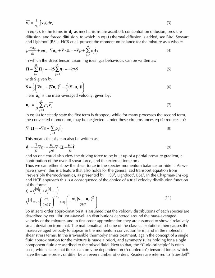
Kirkwood5 and those from irreversible thermodynamics, based on the work of Hirschfelder et al. and De Groot and Mazur5. One of the general impressions is that equations used for the description of rather simple situations, follow logically from these classic equations. We considered the binary counterdiffusion of gases, and Fick’s diffusion experiment of salt in water, and found that simplification of the equations from statistical mechanics for gases and liquids respectively, led to results which were in conflict with experimental observations. We subjected the classic equations from irreversible thermodynamics, to the thought experiment of diffusion through a “mesotrumpet”, and showed that the uncoupling of the shear forces from the mass transfer driving forces, as dictated by the application of the Curie principle, leads to a contradiction with physical reality. A common assumption made in the derivations of these equations in both fields is that one can describe the motion of a fluid mixture as that of a single fluid. In statistical-mechanics derivations this is worked out mathematically by assuming that molecular transport phenomena can be approached as perturbations of the equilibrium molecular velocity distribution functions, which are centered around the mass-averaged velocity. The result is, as it is through assumptions in irreversible thermodynamics, that one can obtain a transport equation for the fluid as a whole in terms of the mass-averaged velocity, and a momentum balance equation for each species in which the shear seems to be absent. The examples we discussed all have in common that phenomena are considered with respect to stationary coordinates, fixed to system walls, and the mathematics show that for isobaric transport in all cases the mass-averaged velocity would be zero, which clearly is not correct. We derived a new approximate solution to the Boltzmann equation for monatomic gases, in which we started with essentially different average velocities for each species. This gives a momentum balances for each species, in which a shearing force for that species occurs side by side with other well-known terms. We proposed a generalized equation, in which thermodynamic non-ideality and bulk viscosity effects were accounted for. With this new type of equation we showed that the problems could be resolved. Due to the nature of the discussed material, there is a lot of specialized mathematics in our paper, making it not easily accessible for everyone interested in multicomponent transport. In the following we will therefore in short show some of the features discussed above. Along with a change in the mathematical approach we found that we needed a change of the conceptual framework of the theory. We have the feeling that this may be very helpful in teaching and studying, and attempt to illustrate this in the second part of the paper. THE CLASSICAL SPECIES MOMENTUM BALANCE It is generally agreed, that molecular diffusion for mixtures in the absence of polymer history terms, should be described by means of the species momentum balance. However, the actual full form of such a balance is hard to find in the textbooks of original workers, such as Chapman and Cowling (CC) or Hirschfelder et al. (HCB), as well as of strong advocates of this principle, such as Wesselingh and Krishna7. For dilute monatomic gases, the results in CC and HCB for the species momentum balance for steady mass transport is given by:

( ) TDDxxxx

j j

Tj

i

Ti

ij

jii

jji

ij

ji ln∇

−−−=− ∑∑ ρρDD

dvv (1)

with the “driving force”:

( ) ( )

−−∇−+∇≡ ∑

jjjiiiiii p

pxx FFd ˆˆ1ln ωρω (2)

Here iv stands for the velocity of i, averaged over its molecular velocity distribution:

∫= iiii

i dfn

vvv 1 (3)

In eq (2), to the terms in id as mechanisms are ascribed: concentration diffusion, pressure diffusion, and forced diffusion, to which in eq (1) thermal diffusion is added, see Bird, Stewart and Lighfoot8 (BSL). HCB et al. present the momentum balance for the mixture as a whole:

∑=

+−∇=⋅∇+∇⋅+∂∂ n

jjjcc

c pt 1

Fuuu

ρρρ ΠΠΠΠ (4)

in which the stress tensor, assuming ideal gas behaviour, can be written as:

SS t

n

jj

n

jj ηη 22

11−=−== ∑∑

==ΠΠΠΠΠΠΠΠ (5)

with S given by:

( ) ( )

⋅∇−∇+∇= IuuuS c

Tcc 3

221 (6)

Here cu is the mass-averaged velocity, given by:

∑=

=n

jjjc

1

1 vu ρρ

(7)

In eq (4) for steady state the first term is dropped, while for many processes the second term, the convected momentum, may be neglected. Under these circumstances eq (4) reduces to2:

∑=

+−∇=⋅∇n

jjjp

1FρΠΠΠΠ (8)

This means that id can also be written as:

iii

ii ppp

pFd ˆ1 ρ

ρρ

−⋅∇+∇= ΠΠΠΠ (9)

and so one could also view the driving force to be built up of a partial pressure gradient, a contribution of the overall shear force, and the external force on i. Thus we can either show the shear force in the species momentum balance, or hide it. As we have shown, this is a feature that also holds for the generalized transport equation from irreversible thermodynamics, as presented by HCB4, Lightfoot9, BSL8. In the Chapman-Enskog and HCB approach this is a consequence of the choice of a trial velocity distribution function of the form:

[ ] [ ]( )[ ] ( )

−−

=

++=

kTm

kTm

nf

ff

ciiiii

iii

2exp

2

..122/3

0

10

uvπ

φ

(11)

So in zero order approximation it is assumed that the velocity distributions of each species are described by equilibrium Maxwellian distributions centered around the mass-averaged velocity of the mixture, and in first order approximation they are assumed to show a relatively small deviation from that. The mathematical scheme of the classical solutions then causes the mass-averaged velocity to appear in the momentum convection term, and in the molecular shear stress terms. In the irreversible thermodynamics treatment, again the concept of a single fluid approximation for the mixture is made a priori, and symmetry rules holding for a single component fluid are ascribed to the mixed fluid. Next to that, the “Curie-principle” is often used, which states that fluxes can only be dependent on (“coupled to”) tensorial forces which have the same order, or differ by an even number of orders. Readers are referred to Truesdell10

for a strong view on this principle and a lot of other terminology used by “Onsagerists”. HCB, followed a little bit differently by Lightfoot9, carry out a complicated development, including the addition of a “zero force”, and obtain a “generalized driving force”:

( )

−−∇−+∇

∂∂

= ∑∑=

≠=

≠

n

jjjiiiii

n

ijj

j

jikxpTj

ii

ti pVcx

xc

RTc k 11,

,,ˆˆ1 FFd ωρωµ

(12)

As we have discussed elsewhere, within their framework, this is identical to:

−∇+∇

∂∂

= ∑≠=

≠

iiii

n

ijj

j

jikxpTj

ii

ti pVcx

xc

RTc k

Fd ˆ1

1,

,,ρµ

(13)

and so, non-ideality in the mixture appears as the gradient in the chemical potential, which replaces the gradient in partial pressure for ideal mixtures, and the occurrence of the term

RTct appears instead of the total pressure p. Krishna11 introduced the notation:

Tpxj

iiijij

n

jiijtpTii

kx

x

xRTcc

,,

1

1,

ln∂∂

+=

∇=∇ ∑−

=

γδΓ

Γµ

(14)

As we have shown in our analysis, also in the work of Bearman and Kirkwood on molecular transport in liquids, the mass-averaged velocity is again taken as frame of reference. The same has been done in developments of plasma transport theory by e.g. Zhdanov12, and many others.

We have shown that for even very simple experimental situations, the classical theory breaks down. One of the examples is the counterdiffusion of two simple gases in a capillary, as studied a.o. by Remick and Geankoplis13, as illustrated in Figure 1. At different absolute pressures they performed isobaric isothermal counterdiffusion experiments, through a bundle

N2 He

x

rpr2

N2 He

x

rpr2

Figure 1. Schematic view of counterdiffusion experiment of He and N2 by Remick and Geankoplis13. Bundle of 644 capillaries, 39.1 µm diameter and 9.6 mm length, temperature 300 K.

of 644 glass capillaries of a length of 0.96 cm, and a diameter of 39.1 µm . From eq (8) follows for isobaric transport in the absence of external forces: ( ) 0=⋅∇ ΠΠΠΠ (14) or in simplified notation for a long cylindrical capillary:

01 , =

−

dr

dur

drd

rxcη (15)

leading even for slip boundary conditions to 0=cxu (16)

and so the mass-averaged velocity would be equal to zero, which is definitely in contradiction to their experiments and those of others such as Graham14. For liquids we found similar problems in the description of the salt diffusion experiments by Fick, and we showed that the equations stemming from irreversible thermodynamics also cannot provide a good description of transport in a channel of given dimensions. As was also observed by Jackson15, the starting equations of Mason et al.16 in their development of the dusty gas model have the same problem as shown in eq (16). This equation was virtually the same as eq (1), but with a slightly different appearance of the factor before the stress tensor2. As we have argued, in situations where the shear force term in the momentum balance cannot be neglected, the approximation of the mixture as one fluid as a whole, breaks down.

In Figure 2 we show the velocities, at the average composition, of the gases used by Remick and Geankoplis, and as we see the species velocities are each larger than the mass-averaged velocity. To be precise, these are the velocities averaged over the molecular velocity distribution, but also over the capillary cross-section. In the classic texts the peculiar ( )iV and

diffusion ( )iV velocities have been introduced:

cii

cii

uvV

uvV

−=

−= (17)

As we see from the figure, for this system the diffusion velocities would be equal to or larger than the mass-averaged velocity, and also physical intuition (or engineering common sense) indicates that it is not useful here to speak of the motion of a fluid mixture.

1 1.4 1.8 2.2 2.6 3 3.4 3.8

1.5

1

0.5

0

-0.5

-1

-1.5

-2

-2.5

-3

-3.5

(m/s) >< xv

2N

He

>< c,xu

( )/Palog10

1 1.4 1.8 2.2 2.6 3 3.4 3.8

1.5

1

0.5

0

-0.5

-1

-1.5

-2

-2.5

-3

-3.5

(m/s) >< xv

2N

He

>< c,xu

( )/Palog10Figure 2. Cross-section averaged velocities of He and N2, and mass-averaged velocity, deduced from the data of Remick and Geankoplis13, evaluated at 50 mol%.

One of the most confusing aspects of many papers and textbooks is that in equations like eq (1) the velocities were replaced by fluxes:

iii cvN = (18) For us as engineers the term “flux” has a strong association with a flow of matter through some given surface area, while a velocity is more associated with a vector at a given point in space. The flux notation was also used by Mason et al. in the derivations of the dusty gas model16, 17, and they provide one example where silently point values are exchanged for fluxes over a cross-section, without any discussion about how to average over the geometry. In general, this has been one of the psychological handicaps of much literature in the field; as chemical engineers we are only too happy if we have equations with fluxes in them, because we can then solve our continuity equations. THE NEW SOLUTION TO THE BOLTZMANN EQUATION From considerations as discussed before, we asked ourselves whether it would be possible to use a “traveling Maxwellian” form for each species as a first order trial function:

[ ] [ ]( )[ ] ( )

−−

=

++=

kTm

kTm

nh

hh

iiiiii

iii

2exp

2

..122/3

0

10

vvπ

φ

(19)

Also, as one can see in problems like the counterdiffusion experiment, we felt that choosing the coordinate system based on the mass-averaged velocity was not desirable, and we kept to stationary coordinates. Indeed we succeeded in obtaining a first-order approximate solution of the Boltzmann equation, and for dilute, monatomic gases the species momentum balance was found to be:

( )

( )

∇

−+−−

∇⋅−+⋅∇+−∇=∂∂

∑∑j j

Tj

i

Ti

ij

ji

jji

ij

ji

iiiiiiiii

i

TDDxxxx

p

pt

ln

ˆ2

ρρ

ρρηρ

DDvv

vvFSv

(20)

Here iη is the partial viscosity of i, and

( )

∇−∇+∇= IIvvvS :

32

21

000 iiT

ii (21)

In our derivation the diffusion term resulted directly from the zero-order approximation. In the Chapman-Enskog approach in the zero-order approximation the average velocities of all components are equal to cu , while in our approach they are different. Eq (20) thus presents an equation of motion for each species, and since they are coupled by the diffusion term, it is a set of simultaneous differential equations. For each component there appears an individual shear term, depending on the individual rate of deformation tensor iS . Molecules i exchange momentum with molecules j, as represented by the diffusion term, but they also exchange momentum with their own kind, resulting in the shear term. Maxwell18 developed the expression for the motion in the x-direction of a species in a binary mixture, his eq (76), which can be written as:

( ) ( ) ( ) xxxzxyxxx Fvvuu

dzd

uudyd

udxd

t

v11,1,22111

21

,11 ˆρρβρρρρρ +−=++

+

∂∂

(22)

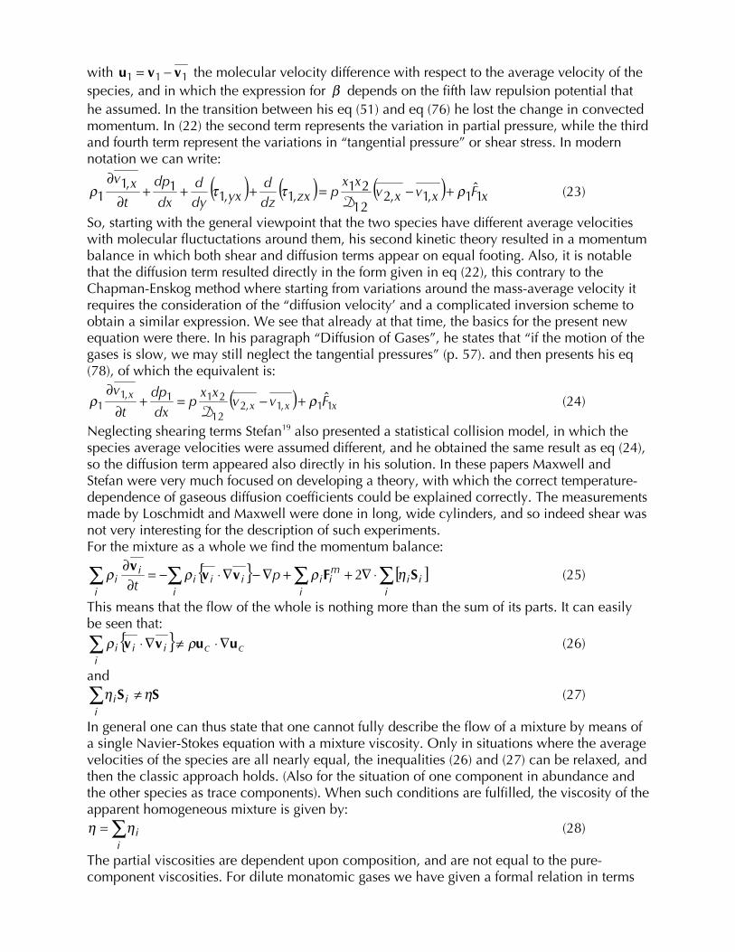
with 111 vvu −= the molecular velocity difference with respect to the average velocity of the species, and in which the expression for β depends on the fifth law repulsion potential that he assumed. In the transition between his eq (51) and eq (76) he lost the change in convected momentum. In (22) the second term represents the variation in partial pressure, while the third and fourth term represent the variations in “tangential pressure” or shear stress. In modern notation we can write:

( ) ( ) ( ) xFxvxvxx

pzxdzd

yxdyd

dxdp

txv

11,1,212

21,1,1

1,11 ρττρ +−=+++

∂

∂

D (23)

So, starting with the general viewpoint that the two species have different average velocities with molecular fluctuctations around them, his second kinetic theory resulted in a momentum balance in which both shear and diffusion terms appear on equal footing. Also, it is notable that the diffusion term resulted directly in the form given in eq (22), this contrary to the Chapman-Enskog method where starting from variations around the mass-average velocity it requires the consideration of the “diffusion velocity’ and a complicated inversion scheme to obtain a similar expression. We see that already at that time, the basics for the present new equation were there. In his paragraph “Diffusion of Gases”, he states that “if the motion of the gases is slow, we may still neglect the tangential pressures” (p. 57). and then presents his eq (78), of which the equivalent is:

( ) xxxx Fvv

xxp

dxdp

t

v11,1,2

12

211,11 ˆρρ +−=+

∂∂

D (24)

Neglecting shearing terms Stefan19 also presented a statistical collision model, in which the species average velocities were assumed different, and he obtained the same result as eq (24), so the diffusion term appeared also directly in his solution. In these papers Maxwell and Stefan were very much focused on developing a theory, with which the correct temperature-dependence of gaseous diffusion coefficients could be explained correctly. The measurements made by Loschmidt and Maxwell were done in long, wide cylinders, and so indeed shear was not very interesting for the description of such experiments. For the mixture as a whole we find the momentum balance:

[ ]∑∑∑∑ ⋅∇++∇−∇⋅−=∂∂

iii

i

mii

iiii

i

ii p

tSFvv

v ηρρρ 2 (25)

This means that the flow of the whole is nothing more than the sum of its parts. It can easily be seen that:

cci

iii uuvv ∇⋅≠∇⋅∑ ρρ (26)

and SS ηη ≠∑

iii (27)

In general one can thus state that one cannot fully describe the flow of a mixture by means of a single Navier-Stokes equation with a mixture viscosity. Only in situations where the average velocities of the species are all nearly equal, the inequalities (26) and (27) can be relaxed, and then the classic approach holds. (Also for the situation of one component in abundance and the other species as trace components). When such conditions are fulfilled, the viscosity of the apparent homogeneous mixture is given by:

∑=i

iηη (28)

The partial viscosities are dependent upon composition, and are not equal to the pure-component viscosities. For dilute monatomic gases we have given a formal relation in terms

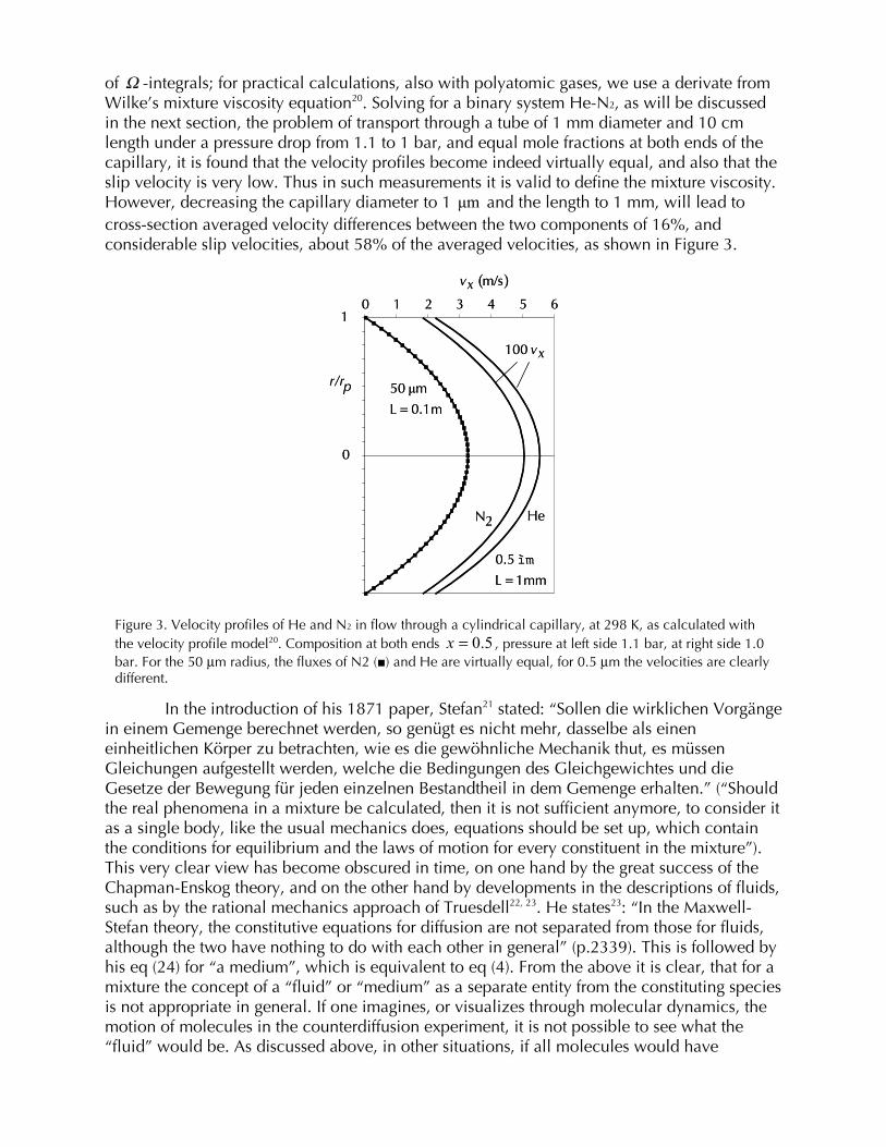
of Ω -integrals; for practical calculations, also with polyatomic gases, we use a derivate from Wilke’s mixture viscosity equation20. Solving for a binary system He-N2, as will be discussed in the next section, the problem of transport through a tube of 1 mm diameter and 10 cm length under a pressure drop from 1.1 to 1 bar, and equal mole fractions at both ends of the capillary, it is found that the velocity profiles become indeed virtually equal, and also that the slip velocity is very low. Thus in such measurements it is valid to define the mixture viscosity. However, decreasing the capillary diameter to 1 µm and the length to 1 mm, will lead to cross-section averaged velocity differences between the two components of 16%, and considerable slip velocities, about 58% of the averaged velocities, as shown in Figure 3.

In the introduction of his 1871 paper, Stefan21 stated: “Sollen die wirklichen Vorgänge in einem Gemenge berechnet werden, so genügt es nicht mehr, dasselbe als einen einheitlichen Körper zu betrachten, wie es die gewöhnliche Mechanik thut, es müssen Gleichungen aufgestellt werden, welche die Bedingungen des Gleichgewichtes und die Gesetze der Bewegung für jeden einzelnen Bestandtheil in dem Gemenge erhalten.” (“Should the real phenomena in a mixture be calculated, then it is not sufficient anymore, to consider it as a single body, like the usual mechanics does, equations should be set up, which contain the conditions for equilibrium and the laws of motion for every constituent in the mixture”). This very clear view has become obscured in time, on one hand by the great success of the Chapman-Enskog theory, and on the other hand by developments in the descriptions of fluids, such as by the rational mechanics approach of Truesdell22, 23. He states23: “In the Maxwell-Stefan theory, the constitutive equations for diffusion are not separated from those for fluids, although the two have nothing to do with each other in general” (p.2339). This is followed by his eq (24) for “a medium”, which is equivalent to eq (4). From the above it is clear, that for a mixture the concept of a “fluid” or “medium” as a separate entity from the constituting species is not appropriate in general. If one imagines, or visualizes through molecular dynamics, the motion of molecules in the counterdiffusion experiment, it is not possible to see what the “fluid” would be. As discussed above, in other situations, if all molecules would have

1

0

6543210

pr/r

2N He

( )m/s xv

xv 100

m 0.1Lm 50

=µ

1mmLìm 0.5

=

1

0

6543210

pr/r

2N He

( )m/s xv

xv 100

m 0.1Lm 50

=µ

1mmLìm 0.5

=

Figure 3. Velocity profiles of He and N2 in flow through a cylindrical capillary, at 298 K, as calculated with the velocity profile model20. Composition at both ends 5.0=x , pressure at left side 1.1 bar, at right side 1.0 bar. For the 50 µm radius, the fluxes of N2 () and He are virtually equal, for 0.5 µm the velocities are clearly different.

approximately the same average velocities and direction, the concept of a fluid seems to be applicable. However, then the simultaneous equations of motion will provide results which show this, as in the 1 mm capillary in Figure 3. THE GENERALIZED MULTICOMPONENT TRANSPORT EQUATION Based upon the monatomic gas equation we have proposed the following generalized transport equation:

( ) ( ) IvSvv

Fvvv

iiii

n

jij

ij

jit

n

j j

Tj

i

Ti

ij

jit

iiiiipTiiiii

i

xxRTcT

DDxxRTc

pVcct

⋅∇+⋅∇+−+∇

−−

+∇−∇−∇⋅−=∂∂

∑∑==

ϕηρρ

ρµρρ

2ln

ˆ

11

,

DD

(29)

in which the partial pressure gradient has been replaced by the gradient of the chemical potential, and the bulk viscosity term has been added. The total pressure has been replaced by RTct . Addition over all components gives the equivalent of eq (25), but now with the bulk

viscosity effects in addition:

( ) ∑∑∑∑ ⋅∇+⋅∇++∇−∇⋅−=∂∂

iiiii

iii

iiii

i

ii p

tIvSFvv

v ϕηρρρ 2ˆ (30)

For the steady transport of a binary mixture in a long flat channel or long capillary, under isothermal conditions, absence of external forces, neglecting bulk viscosity effects and change in convected momentum, eq (29) goes over in the equations of the earlier velocity profile model 1 (VPM-1)20. For gases this reads:

( )xxx vv

xxp

r

vr

rrdxdp

,2,112

21,11

1 1 −−

∂∂

∂∂=

Dη (31)

( )xxx vv

xxp

r

vr

rrdxdp

,2,112

21,22

2 1 −+

∂∂

∂∂=

Dη (32)

We have solved this set of simultaneous differential equations analytically for the two geometries, using Maxwell slip boundary conditions. These will be discussed in the next section. For the analytical expressions the reader is referred to2, 20. The result is the velocity profile of each species over the radius, as shown in Figure 4. Integration over the cross-section gives then information about the cross-section-averaged velocities >< xiv , . We found that we could, for this simple type of problem, invert the resulting equations into:

( ) 1,11,2,112

211 pvfvvxpx

gdxdp

xmxxD ><−><−><−=D

(33)

( ) 2,22,1,212

212 pvfvvxpx

gdx

dpxmxxD ><−><−><−=

D (34)

The equation resembles the Maxwell-Stefan equation, but in the diffusion term the diffusion averaging factor Dg appears which accounts for the fact that using the difference in averaged velocities is not equal to the average of the velocity differences. The last terms represent the friction with the wall, and also for the imf equations follow from the derivation. Only after this rather complete result, we make the transition to the species fluxes:

RTp

vcvN ixiixixi >=<>>=<< ,,, (35)

and we obtain:

( )

( ) ><−><−><−=

><−><−><−=

xmxxD

xmxxD

NRTfNxNxRT

gdx

dp

NRTfNxNxRT

gdxdp

,22,12,2112

2

,11,21,1212

1

D

D (36)

In applying this to the continuity equation for the counterdiffusion problem, we have the problem that the partial pressures (compositions), the Dg and the imf are varying along the length of the tube. At specified end partial pressures this forms a boundary value problem, which we solved by means of iteration20, 24. In Figure 5 we have plotted the fluxes we calculated for the Remick and Geankoplis experiments against the experimental data, and we see excellent agreement. In earlier work we have more on basis of engineering intuition, set up a model directly for the averaged fluxes, the binary friction model (BFM)24. The above strongly supports this model, be it that the averaging factor Dg was not present there. For gases the imf are numerically equal to those of the BFM, while for liquids the equations are identical. Depending on the situation, certain terms in the equation of motion may be more important than others. For a binary system in a long channel, as described by eq (31) and (32), we derived a modulus:

pt KxRTxc121

21

12ηηηϕ D= (37)

with 8

2p

pr

K = for cylindrical channels, and 3

2p

pr

K = for flat channels. This modulus can be

seen as a measure for the ratio of the shear forces and the interspecies diffusive friction forces. A small value of ϕ means that the influence of the shear terms is small, a large value that it is dominating. In the case of small ϕ , the collisions between molecules i and j are much more

0 1

0.4

0

-0.5

-0.8r/R

0.15 kPa

3 kPa

40 kPa

>∞<>< x,MS,v/xv

0.15 kPa

3 kPa

40 kPa

2N

He

0 1

0.4

0

-0.5

-0.8r/R

0.15 kPa

3 kPa

40 kPa

>∞<>< x,MS,v/xv

0.15 kPa

3 kPa

40 kPa

2N

He

Figure 4. Calculated relative species velocity profiles for capillaries as used by Remick and Geankoplis13. Reference velocity is the velocity difference for an infinite medium2. Parameter is the total pressure: (a) 0.15 kPa, (b) 3 kPa, (c) 40 kPa.

frequent than those between i and i, this tends to bring the average velocities of both species close together. For large ϕ , the momentum exchange between faster and slower molecules i, and similarly for j, tends to make the differences in average velocities larger. We have also presented the equation of energy as follows from the new Boltzmann solution, as well as the generalized version2.

ON TEACHING AND STUDYING MULTICOMPONENT TRANSPORT When confronted with the host of papers, textbooks and teaching material, students and many professors alike, are made aware of the importance of the momentum balance7, 25,

26. However, the species motion is mainly written in terms of fluxes, and in the balance the shear term does not appear. The difference between point and space-averaged fluxes is not explained. Elucidations are made, that these results stem from statistical mechanics or from irreversible thermodynamics. This, together with the very cumbersome discussions about fluxes and forces, and mathematical inversions, has made the teaching of multicomponent transport more a descriptive than a logical activity, and from the consumers faith is asked rather than physical understanding. Until now. What we would like to show here is a different framework for teaching and studying these phenomena. Matters have also been complicated because in considering the flow of gases through tubes, the concept of slip velocity is hardly discussed in the textbooks on transport phenomena. For that reason we start with considering the flow of a single gas first, after which we will discuss the counterdiffusion example, and see that we can also apply engineering reasoning to obtain multicomponent transport equations. Steady isothermal dilute gas transport in a capillary tube: wall slip and Knudsen flow As stated above, one of the confusing factors in considerations of gas flow through pores and tubes is the phenomenon of wall slip, which is not generally taught in transport phenomena textbooks. For flow of a liquid along a wall, such as in a tube, in most common situations one may assume the no-slip condition, i.e. the fluid velocity at the wall is equal to

-0.5 -0.3 -0.1 0.1

0.2

0.1

0

-0.1

-0.2

-0.3

-0.4

-0.5

>< s2kmol/m3-10expi,N

>< s2kmol/m3-10i,thN

2N

He

-0.5 -0.3 -0.1 0.1

0.2

0.1

0

-0.1

-0.2

-0.3

-0.4

-0.5

>< s2kmol/m3-10expi,N

>< s2kmol/m3-10i,thN

2N

He

Figure 5. Fluxes of He and N2 in counterdiffusion experiment of Remick and Geankoplis13; comparison between results from velocity profile model (VPM-1) and experimental values.

zero. As discovered experimentally by Kundt and Warburg in the 1850’s, a dilute gas flows like it is slipping at the wall, so there appears a positive velocity along the wall. Maxwell27 provided an explanation for this, and a corresponding theoretical basis. Molecules which hit the wall will not all reflect as like a light ray in a mirror (specular reflection), but also may reflect in any possible direction (diffuse reflection). Maxwell pictured this as a surface of closely packed spheres. The probability that a molecule will after collisions with the wall have the same tangential velocity direction as before the impact is greater than that of the opposite. When there is a net flow of the gas to one side, thus more molecules will be reflected in the direction of this flow. After collision with the wall atoms, the molecules will travel on the average the mean free path, and collide with the molecules in the core of the tube. For the core flow this means that it “feels” not a zero velocity at the wall, but a net velocity. Mathematically Maxwell derived expressions for the averaged velocities of both specular and diffuse reflection, and for the shear near the wall, leading for a capillary tube to the expression, including thermal slip:

043 =−

∂∂

+dxdT

Trv

Gv xx ρ

η (38)

Here G is the slip modulus (“Gleitmodulus”). Maxwell derived:

Λ

−= 12

32

fG (39)

in which Λ is the mean free path, and f is the fraction of molecules which is reflected diffusely. Now let us make some simplifying assumptions for the equation of motion for the single component. Generations of chemical engineers have profited from the wonderful text by BSL, in which they showed for a host of interesting situations how one can simplify a.o. the Navier-Stokes equations, and derive approximate solutions. The first step in this is that we consider special symmetries, with the aid of which we may scratch out certain terms. In the case of steady transport, as zero-step we scratch out the time-dependence, since we have steady flow, and the external force since we think gravity has hardly any influence. It should be noted however, that the assumption, or condition, of steady flow is always dependent on the coordinate system chosen. In the present case we naturally choose to fix our coordinate system with respect to the capillary tube. We may assume that the flow will be axi-symmetrical, and there will be no dependence on the angle θ . A bit more complex is the next step. Since the capillary is assumed to be very long, we assume that the velocity profile has developed, and that we can neglect the velocity changes at the inlet (entrance effects). Also, we assume for the same reason, that we have no radial pressure differences, and there is no radial velocity. Further we will assume isothermal transport, neglect bulk viscosity effects, and change of convected momentum. As is usual, we assume that the axial velocity depends much stronger on the radial coordinate than on the axial coordinate. Let us apply this for a long cylindrical capillary, and by scratching out terms we obtain:

01 =

+−

drdv

rdrd

rdxdp xη (40)

Because of the assumptions, we have now changed the partial differentiation to single

differentiations, so dxdp

does not depend on r, and xv depends much stronger on r, than on x.

So, now we have a differential equation, and since dxdp

does not depend on r, we can

integrate this as:

2

2

41

Cr

dxdp

vx +

=

η (41)

Up to here this is simple standard textbook work. Now we apply the Maxwell slip boundary condition:

drdv

Gvrr xxp −== (42)

Application of this boundary condition gives:

( )ppx Grrrdxdp

v 241 22 +−

−=

η (43)

For the total volumetric flow rate we obtain:

( )ppp

r

xv Grrr

dxdp

rdrvp

48

2 22

0

+

−== ∫ η

ππφ (44)

For the average velocity over the cross-section we have:

+

−=>=<

p

p

p

vx r

Gr

dxdp

rv

418

2

2 ηπφ

(45)

Now let us consider the slip-modulus. It has the dimension of length, and is related to the mean free path Λ . Knudsen28 performed experiments on the flow of various gases through capillaries, in which he determined the flux as a function of the pressure difference, at different levels of the average absolute pressure. As will be discussed further on, the Maxwell relation provides a good fit, but does not describe precisely the measurements at extremely low pressures. Fitting to Knudsen’s measurements, we find that:

4.11

1≈=

CCG Λ

(46)

This would correspond to a fraction 65.0=f for diffuse reflection, which may be compared with 5.0=f , as found by Maxwell on the basis of the experiments of Kundt and Warburg with air in glass. The mean free path can be expressed as:

n221πσ

Λ = (47)

in which σ is the collison diameter of the molecules, and n is the number density [molecules/m3]. We can relate this to other physical properties by:

K

pD

prMRT

pG η

πη 2819.1

2/1=

≈ (48)

Here KD is the Knudsen “diffusion” coefficient; rather it should be called Knudsen flow coefficient. It is given by:

2/1

0

0

832

89.0

=

≈

MRT

rD

DD

pK

KK

π

(49)

Again, the factor 0.89 comes from fitting to the experimental data. We substitute eq. (48) into (47) to obtain:

+

−>=<

pDr

dxdp

vKp

x η8

2

(50)

Next we introduce at this point the molar flux:

iii cvN ≡ (51) For the averaged molar flux (so over the cross-section), we find:

+

−=>=<>>=<< Kp

xtxx Dpr

dxdp

RTRTp

vcvNη8

12

(52)

We can integrate this over the length of the tube L, taking into account that at steady flow the molar flux is constant over the length, and then we obtain:

RTLp

Dpr

N KLav

px

∆η

+>=< ,

2

8 (53)

in which

( )LxxLav ppp == += 0, 21 (54)

Equation (38) suggests that if we make a plot of pNx ∆/>< versus the average pressure

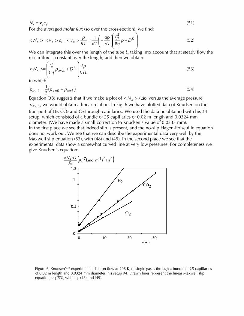
Lavp , , we would obtain a linear relation. In Fig. 6 we have plotted data of Knudsen on the transport of H2, CO2 and O2 through capillaries. We used the data he obtained with his #4 setup, which consisted of a bundle of 25 capillaries of 0.02 m length and 0.0324 mm diameter. (We have made a small correction to Knudsen’s value of 0.0333 mm). In the first place we see that indeed slip is present, and the no-slip Hagen-Poiseuille equation does not work out. We see that we can describe the experimental data very well by the Maxwell slip equation (53), with (48) and (49). In the second place we see that the experimental data show a somewhat curved line at very low pressures. For completeness we give Knudsen’s equation:

0 10 20 30

1.2

1

0.5

0

(kPa)

( )1-Pa 1-s 1-m kmol7-10 Äp

LxN ><

2H2CO

2O

0 10 20 30

1.2

1

0.5

0

(kPa)

( )1-Pa 1-s 1-m kmol7-10 Äp

LxN ><

2H2CO

2O

Figure 6. Knudsen’s28 experimental data on flow at 298 K, of single gases through a bundle of 25 capillaries of 0.02 m length and 0.0324 mm diameter, his setup #4. Drawn lines represent the linear Maxwell slip equation, eq (53), with eqs (48) and (49).

Lav

LavKKpa

paDD

,2

,10 1

1++

= (55)

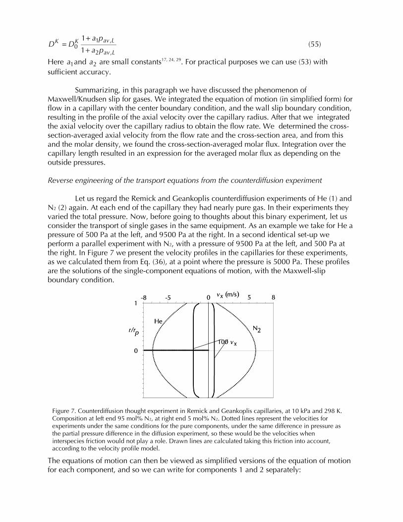
Here 1a and 2a are small constants17, 24, 29. For practical purposes we can use (53) with sufficient accuracy. Summarizing, in this paragraph we have discussed the phenomenon of Maxwell/Knudsen slip for gases. We integrated the equation of motion (in simplified form) for flow in a capillary with the center boundary condition, and the wall slip boundary condition, resulting in the profile of the axial velocity over the capillary radius. After that we integrated the axial velocity over the capillary radius to obtain the flow rate. We determined the cross-section-averaged axial velocity from the flow rate and the cross-section area, and from this and the molar density, we found the cross-section-averaged molar flux. Integration over the capillary length resulted in an expression for the averaged molar flux as depending on the outside pressures. Reverse engineering of the transport equations from the counterdiffusion experiment Let us regard the Remick and Geankoplis counterdiffusion experiments of He (1) and N2 (2) again. At each end of the capillary they had nearly pure gas. In their experiments they varied the total pressure. Now, before going to thoughts about this binary experiment, let us consider the transport of single gases in the same equipment. As an example we take for He a pressure of 500 Pa at the left, and 9500 Pa at the right. In a second identical set-up we perform a parallel experiment with N2, with a pressure of 9500 Pa at the left, and 500 Pa at the right. In Figure 7 we present the velocity profiles in the capillaries for these experiments, as we calculated them from Eq. (36), at a point where the pressure is 5000 Pa. These profiles are the solutions of the single-component equations of motion, with the Maxwell-slip boundary condition.

The equations of motion can then be viewed as simplified versions of the equation of motion for each component, and so we can write for components 1 and 2 separately:

850-5-8

0

pr/r

1

2NHe

( )m/s xv

x v100

850-5-8

0

pr/r

1

2NHe

( )m/s xv

x v100

Figure 7. Counterdiffusion thought experiment in Remick and Geankoplis capillaries, at 10 kPa and 298 K. Composition at left end 95 mol% N2, at right end 5 mol% N2. Dotted lines represent the velocities for experiments under the same conditions for the pure components, under the same difference in pressure as the partial pressure difference in the diffusion experiment, so these would be the velocities when interspecies friction would not play a role. Drawn lines are calculated taking this friction into account, according to the velocity profile model.

[ ] [ ][ ] [ ] 222,2222

22

111,11111

1

ˆ2

ˆ2

FSvvv

FSvvv

ρηρρ

ρηρρ

+⋅∇+∇−∇⋅−=∂∂

+⋅∇+∇−∇⋅−=∂∂

pure

pure

pt

pt (56)

For He we have no bulk viscosity term, since it is a monatomic gas, and for N2 we assume that the term can be neglected. We have:

( ) ( )

⋅∇−∇+∇= IvvvS i

Tiii 3

221 (57)

So, for the separate components we see that there is slip at the wall, and that due to shear the velocity at the wall is smaller than that at the center. The dynamic viscosities pure,1η and

pure,2η of the two components are different, as they represent the momentum exchange between faster and slower molecules of each species, with their respective masses and intermolecular attraction potentials. Now, let us do a first step towards the description of the Remick and Geankoplis experiment for the mixture. If the molecules of (1) and (2) would not influence each other, we would expect the undisturbed velocity profiles of each species, as sketched in Figure 7. Of course, this is an unrealistic approach, since molecules (1) and (2) will also collide, and since they are on the average moving in different directions, they will retard each other. Thus it seems logical to account for this by the introduction of an intermolecular friction force in each equation of motion (which is equivalent to the species momentum balance). We now make the assumptions as done by Stefan21, be it that he did not consider shear. The force on (1) per unit total volume is assumed to be proportional with the molar concentration of (1), with that of (2), and with the difference in average velocities. We can express this in the following form:

[ ] [ ] ( )

[ ] [ ] ( )2112

212222222

22

1212

211111111

11

ˆ2

ˆ2

vvFSvvv

vvFSvvv

−++⋅∇+∇−∇⋅−=∂∂

−++⋅∇+∇−∇⋅−=∂∂

D

Dxx

ppt

xxpp

t

ρηρρ

ρηρρ (58)

Thus in order to solve this binary transport problem, we have to solve the two simultaneous equations of motion, with appropriate boundary conditions. The introduction of the effective friction between (1) and (2) does not eliminate the shear due to radial differences in velocity for each component, and it also does not remove wall slip effects. However, we can expect that the molecular velocity distributions of each species are different from the single-component distributions, due to the interspecies collisions, and so the viscosities that appear should be functions of composition, and are not equal to the pure-component viscosities. As has been discussed in some more detail before, 1η and 2η are partial viscosities. The shear terms for each component only include the gradients in the velocity of the components themselves; the interspecies collisions are accounted for in the last new term. In earlier work we found a simplified set of such equations for transport in circular capillaries and flat channels20. The above reasoning leading to eq. (58) may seem to be a bit simplistic in nature. However, we are in the good company of Stefan. Moreover, it is in full accordance with the isothermal generalized solution eq (20) of the Boltzmann equation, if we neglect bulk viscosity. Of course, we can extend (58) also to multicomponent systems. As yet, we have not developed analytical solutions for the transport in a capillary for more than two components. However, as we have seen that for a binary system the general theory developed here fully supports the binary friction model, we suspect that this will also describe ternary systems with good accuracy. In the same set-up as used for binary gas diffusion,

Remick and Geankoplis30 also performed isobaric measurements on ternary systems of He, Ne and Ar, at different absolute pressure levels. In Figure 8 a comparison is made between the data as predicted by the BFM, and the experimental data. Excellent agreement is observed again. Introductory numerical solutions of the simultaneous equations of motion for the ternary system in a long capillary, gave results which correspond very well with the BFM predictions.

Maxwell-Stefan equations in the absence of shear With eq (29) as a starting point, a first simplification we can make is to assume that acceleration can be neglected. However, it also means that we have to state with respect to which coordinate system. If we would travel at steady speed through the diffusion capillary, we would definitely see a change of the iv with time. Thus for such an experiment we define the coordinate system as fixed with respect to the capillary. A following simplification could be that shear can be neglected. We have to justify this, because it means that there will be no velocity gradients. For a drying droplet of a food liquid in a spray dryer, we may assume that stresses are minimal, and we choose the coordinate fixed with respect to the droplet center. For a wide tube, under non-turbulent conditions, we may expect shear to be much smaller than the diffusive friction force. A third assumption we could make, is that the change in convected momentum is small with respect to the other forces. Under these three assumption, we obtain from eq (29):

( ) 0

lnˆ

1

1,

=−+

∇

−−+∇−∇−

∑

∑

=

=

n

jij

ij

jit

n

j j

Tj

i

Ti

ij

jitiiiiipTi

xxRTc

TDDxx

RTcpVcc

vv

F

D

D ρρρµ

(59)

and for the summation over the mixture: 0ˆ =+∇− ∑

iiip Fρ (60)

610−510− 410− 310−

He

Ne

Ar

s)2(kmol/m >< i,xNBFMi,xN ><

expi,xN ><610−

510−

410−

310−

610−510− 410− 310−

He

Ne

Ar

s)2(kmol/m >< i,xNBFMi,xN ><

expi,xN ><610−

510−

410−

310−

Figure 8. Ternary isobaric diffusion experiments of Remick and Geankoplis30 with He, Ne and Ar, in the same equipment they used for binary experiments, at 300 K and varying total pressure. Comparison of predictions from binary friction model with experimental data.

Eq (60) is very interesting; if we assume that shear does not play a role, or equivalently that we have virtually no velocity gradients, it means that we can only have a pressure gradient under the influence of external forces. If, as a fourth assumption, we neglect those, such as gravity, a system without velocity gradients and external forces would be isobaric. Let us imagine that we apply these assumptions to the isothermal transport in a tube, say a Stefan-tube. The fact that we assume no radial gradients of the axial velocities, deprives us of the possibility of solving the simultaneous equations of motions for water and air. We have left of the equations now:

( )

( ) 0

0

1212

212

2112

211

=−−∇−

=−−∇−

vv

vv

D

Dxx

pp

xxpp

(61)

What we do in the classic undergraduate problem is assume that the air is stationary with respect to the tube, so we fix one velocity. Also, because the system has become isobaric, we have only one independent partial pressure left. Thus both in velocities and in partial pressures we have reduced the system to one variable less. Duncan and Toor31 performed isothermal ternary diffusion experiments through a wide-bore capillary tube, of 8.59 cm long and 2.08 mm diameter, connecting two bulbs of 78 cm3, filled initially with different gas mixtures. Again, it is reasonable to assume quasi-steady flow through the tube, and also to neglect convected momentum. Making the assumption that shear can be neglected, again leads to the consequence of isobaric transport. According to the equation of continuity, we have for the mixture as a whole:

[ ]ttt

cN⋅∇−==

∂∂

0 (62)

or for transport in a long tube:

0, =dx

dN xt (63)

and so we would have a constant total flux in the axial direction. For the system of Duncan and Toor, the most reasonable assumption to make is then that the total flux equals zero. A non-equimolar transport would immediately lead to a pressure difference between the two bulbs, which would be taken away very rapidly, because we assume there is no shear. Thus we have again decreased the number of independent partial pressures by one, as well as the number of independent velocities (or fluxes). When considering diffusion of water and solutes during drying of foods, or diffusion of salt in water, molecular volume contraction is small, and so we assume equivolumetric transport2, 32. For a multicomponent system under the conditions mentioned here, we can then also write it in Fickian form for ( )1−n components:

( ) ( ) ( ) ∑∑−

=

−

=∇−=∇−=

1

1

1

1

n

ji

Fijtt

n

ji

Fijt xDcxcDx NNN (64)

as shown by Taylor and Krishna25. Here we have adopted their notation:

( ) ( )

=

=

−− 1

2

1

1

2

1

:,

:

nn x

xx

x

N

NN

N (65)

The matrix of Fickian diffusion coefficient can be written as:

[ ] [ ] 1−= BDF (66) with the elements given by:

∑−

≠=

+=

≠

−=

1

1

11

n

ikk ik

k

in

iii

ijiniij

xxB

jixB

DD

DD (67)

They show that the Fickian diffusion coefficients are not symmetrical Fji

Fij DD ≠ , contrary to

the Maxwell-Stefan coefficients. A further note on this is that for the isobaric equations, we have for gases:

iit

iti pRT

xRTp

xcc ∇=∇=∇=∇ 1 (68)

Thus one of the questions raised by Do33, what the correct shape of the Maxwell-Stefan equation is, has been answered. The different forms he discusses are all equal because the system is isobaric due to the (implicit) assumptions. If we consider a liquid system, neglecting acceleration, change in convected momentum, and assume that shear can also be neglected, we can invert eq (59) to obtain:

( ) ( ) [ ] [ ]( ) ( ) ( ) ( )[ ]TRTâPVcxRTcBRT

x Ttt lnˆ1 1 ∇+−∇+∇−= − FNN ρΓ (69)

with

∑=

−=

n

j j

Tj

i

Ti

ij

jit

Ti

DDxxc

1 ρρβ

D (70)

and so, if one likes, one could say that the flux of a component is influenced by the total flux, by a gradient in concentration, by the total pressure gradient, by external forces and by the temperature gradient. Eq (69) has the advantage that it can be used in the continuity equation. However, it only holds under the given assumptions, in the absence of shear. A steady mixture in a gravitational field Let us consider an equilibrium system in a gravitational field; for this the average velocity of the species are equal to zero. From the general equation we obtain for an isothermal mixture in a system without velocity gradients:

0ˆ, =+∇−∇− iiiiipTi pVcc Fρµ (71) Addition over all components gives:

0ˆ1

=+∇− ∑=

n

iiip Fρ (72)

For a gravitational field: gF =iˆ (73)

leading to 0=+∇− gρp (74)

Substitution in (71), and using (13) again:

( )ii

n

ijijt

ii

n

ijijt

xRTc

xRTc

φωρΓ

ρρφΓ

−=∇

=+−∇−

∑

∑

=

=

g

gg

1

10

(75)

For an ultracentrifuge we have: r2ω=g (76)

and so:

( )ii

n

ijijt rxRTc φωρωΓ −=∇∑

=

2

1 (77)

What we demonstrate here is that the derivation is much easier than that in textbooks, such as Taylor and Krishna25, because the confusing artificial driving force as in eq (12) is not introduced. CONCLUDING REMARKS One of the main conceptual points that we have made here, is that solving a multicomponent molecular transport problem comes down to the solution of a set of simultaneous equations of motion, coupled with the equations of continuity, and where needed with the equation of energy. The general equations of motion are momentum balances of the forces acting on the amounts of a component per unit volume, and contain terms in which the chemical potential gradient, the temperature gradient, interspecies friction and intra-species shear all play a role. To solve the set, in general boundary conditions are needed. The solution will provide both velocities and concentrations of each component in space and time. For steady flow, neglecting change in convected momentum, and for negligible shear, a subclass of equations of motion is obtained, the various types of earlier presented Maxwell-Stefan equations, in which no “lateral” velocity gradients are present, and consequently no boundary conditions at walls can be fulfilled, thus degrading the set to ( )1−n simultaneous equations, requiring one additional specification for the velocities (fluxes), and containing a condition for the total pressure gradient. It is up to the scientist to determine when such assumptions are reasonable. In our framework thus the species velocities are the main parameters describing the species motion, and fluxes come in a late stage, when everything else is known. In the mentioned review in the introduction, Bird1 poses question “h” as one of the area of further investigation: “What is the correct velocity boundary condition at the tube wall when a homogeneous mixture is flowing through the tube? Does the mass-average velocity equal zero, or the molar average, or the volume average?” Our answer is that principally there is no possibility of a fluid mixture flowing along a wall to remain homogeneous, because there will operate different shearing forces for the different species. As we have shown, only when shear plays a very minor role, the concept of a homogeneous fluid can be a good approximation. Looking back, we feel amazement about the long-time extreme state of confusion in the area of multicomponent transport in capillaries and pores. We can summarize this as: “A pore is a black hole, from which scientific information about what is going on inside, cannot escape.” The engineering community has thus devised a large number of simple approximations, such as the Bosanquet equation, the Geankoplis equation, and others, for which it was stated that momentum conservation was the basis. However, nowhere the shear appeared. Renowned physicists such as Mason et al. have developed the dusty gas model, but

needed some erroneous steps in an attempt to repair the faults of their starting equation. Zhdanov and Roldughin have written studies specially devoted to transport in capillaries12, 34,

35, in which they do not provide a closed solution, probably because their starting equation is the same as that of Mason, and so will not lead to sensible results. Although much interesting work remains to be done, such as a more detailed consideration of the slip boundary conditions, we have shown that from a general formulation of the equations of motion, solutions can be obtained by either analytical mathematics or numerical methods, regular tools in chemical engineering. We have also shown earlier that this new attack enables the modeling of liquid ultrafiltration in membranes with small pores []. The conceptual change of frame also makes many of the classic terms and treatments, such as “osmotic diffusion”, “viscous selectivity”, “non-segregative fluxes”, the use of inert porous membranes or solids as one of the components, “diffusion velocity”, and “generalized driving force”, obsolete. In our opinion the book on the dusty gas model should finally be closed, including the extremely confusing arguments on which diffusion coefficient are the “true” ones, and which are “augmented” ones26, 36, 37. Just like in thermodynamics, the scientist has to define how many phases and components there are; thus for inert membranes with meso-pores the solid phase is to be regarded as a wall, and not as a mixture component. For transport between adsorbing or absorbing solids, a clear definition of phases is again one of the duties of the scientist involved, as is a precise picture of the way the transport in the adsorbed phase is envisioned to take place. The intrinsic role of the shear force in the equations of motion was found directly from the non-equilibrium approximate solution of the Boltzmann equation for dilute monatomic gases. The transport theory from irreversible thermodynamics is at present not able to describe this relatively simple system. The collisions between atomic molecules show microscopic time-reversibility, which is also one of the Onsager starting points. We see it as a challenge to reconsider the derivations and see how the two developments can be united. The development of the theory around the individual species averaged velocities is crucial for obtaining the type of equations of motion including the individual shear terms. In retrospect, it is remarkable to see that the pioneers Maxwell and Stefan both used this as their starting point, and that the attention for this virtually vanished after the Chapman-Enskog and Hirschfelder et al. solutions of the Boltzmann equation. As indicated, Maxwell obtained this specific shear force in his derivations for binary diffusion, and we obtained it from our more general solution of the Boltzmann equation. It is clear, that we were only able make our derivations because of the tremendous mathematical work of the scientists before us. In all modesty, we must observe that only after all our work on statistical mechanics had been done, we were able to understand the derivations of Maxwell and see the significance of his eq (76), which eluded us at earlier readings. We reached the conclusion that a mixture can in general not be treated as a single fluid after a lot of thought, and only afterwards on reading Stefan again, the meaning of his introductory words became clear to us. Also, it is only now that we see the term “equation(s) of motion” in the works of the early scientists in the field, when they presented their momentum balances3, 18. Thus, although a lot of our work may be regarded as “new”, some basic insights were already present for those to see since over 130 years. With the new transport equation we have extended the tools for rational modeling in areas where this was not possible before. Thus we feel that we have contributed to broadening the basis of transport phenomena. We have given a modest indication about how one could teach and understand molecular transport on a rational basis. Since the theory is generally applicable for isotropic systems, it is certainly not limited to pores or tubes, but can

be used to model a large variety of more-dimensional situations. Within the field of chemical engineering we can think of CVD- and micro-reactors, transport in nanotubes, but also the essentially more-dimensional transport in meso- and macropores in catalysts and adsorbents. Possibly the mode of attack can also be of use in plasma physics. Scientifically, reinvestigation of derivations for dense fluids, polyatomic gases, and polymeric liquids along the lines we have followed, would be very interesting. Thus, in the spirit of Feynman38, when he discussed open areas of research, especially devoted to “nanomachines”, we may paraphrase: “There’s plenty of room at the bottom of transport phenomena”. Notation

21,aa constants, eq (55) [N-1 m2] [B] inverse diffusion matrix, eq (67) [m-2 s]

1C constant, eq (46) [-] 2C integration constant, eq (41) [m s-1]

c molar concentration [kmol m-3] D Fickian diffusion coefficient [m2 s-1]

KD Knudsen coefficient [m2 s-1] TiD thermal diffusion coefficient [kg m-1 s-1] ijD Maxwell-Stefan diffusion coefficient [m2 s-1]

id driving force, eq (1), (2), (12) [m-1]

iF force per kg i [N kg-1] f molecular velocity distribution function [molecules m-6 s3] f diffuse reflection fraction [] imf wall-friction coefficient, eq (33) [m-2 s]

iG slip modulus [m] g gravitational acceleration [m s-2]

Dg diffusion averaging factor [-]

ih velocity distribution function in new theory2 [molecules m-6 s3] I diagonal unit tensor [-]

pK channel permeability [m2] k Boltzmann’s constant [J K-1] L length [m] M molar mass [kg kmol-1] m molecular mass [kg molecule-1]

N,N molar flux with respect to fixed coordinates [kmol m-2 s-1] n molecular density [molecules m-3] n number of components [-] p pressure [Pa]

R gas constant [J kmol-1 K-1] r coordinate [m] pr channel radius or width [m]

S rate of deformation tensor [s-1] T temperature [K]

u,u velocity [m s-1] V relative velocity, eq (17) [m s-1]

V specific volume [m3 kmol-1] v,v velocity [m s-1] x mole fraction [-] x Cartesian coordinate [m] y Cartesian coordinate [m] z Cartesian coordinate [m] Mathematical <> area-averaged

ia quantity a , averaged over velocity distribution of i [*] Greek β Maxwell friction parameter, eq (22) [kg-1 m-3 s-1]

Tiβ thermal coefficient, eq (70) [kmol m-3] ijδ Kronecker delta [-]

φ perturbation function [-] iφ volume fraction [-] vφ volumetric flow rate [m3 s-1] ϕ bulk viscosity [Pa.s] ϕ modulus, eq (37) [-] Γ thermodynamic factor, eq (14) [-] γ activity coefficient [-] η dynamic viscosity [Pa.s]

iη partial dynamic viscosity [Pa.s] tη mixture dynamic viscosity [Pa.s] Λ mean free path [m] µ chemical potential [J kmol-1] ΠΠΠΠ stress tensor, eq (5) [Pa] ρ concentration, density [kg m-3] σ molecular diameter [m] τ shear stress [Pa] ω mass fraction [-] ω angular velocity [rad s-1] Subscripts 1,2 species 1 resp. 2 c mass-averaged p constant pressure pure for pure component T constant temperature t total x,y,z in x,y,z-direction

Superscripts [0] zero-order approximation [1] first-order approximation D diffusive F Fickian T transpose Literature Cited 1. Bird RB. Five Decades of Transport Phenomena. AIChEJ, 2004;50:273-287. 2. Kerkhof PJAM,Geboers MAM. Towards a Unified Theory of Isotropic Molecular Transport Phenomena. AIChEJ, 2004, in press 3. Chapman S, Cowling TG. The Mathematical Theory of Non-Uniform Gases (3d edition). Cambridge: Cambridge University Press, 1970. 4. Hirschfelder JO, Curtiss CF, Bird RB. Molecular Theory of Gases and Liquids (2nd printing). New York: John Wiley & Sons, 1964. 5. Bearman, RJ, Kirkwood JG. Statistical Mechanics of Transport Processes. XI. Equations of Transport in Multicomponent Systems. J. Chem. Phys. 1958;28:136-145. 6. De Groot SR, Mazur P. Non-Equilibrium Thermodynamics. New York: Dover Publications, 1984. 7. Wesselingh JA, Krishna R. Mass Transfer in Multicomponent Systems. Delft: Delft University Press, 2000. 8. Bird RB, Stewart WE, Lightfoot EN. Transport Phenomena (2nd edition). New York: John Wiley & Sons, Inc., 2002. 9. Lightfoot EN. Transport Phenomena and Living Systems. New York: Wiley-Interscience, 1974. 10. Truesdell C. The Onsager Relations. In Truesdell C. Rational Thermodynamics, 2nd edition. New York: Springer-Verlag, 1984: 365-404. 11. Krishna R. A Unified Theory of Separation Processes Based on Irreversible Thermodynamics. Chem. Eng. Comm. 1987;59:33-64. 12. Zhdanov VM. Flow and Diffusion of Gases in Capillaries and Porous Media. Adv. Colloid Interf. Sci. 1996;66:1-21. 13. Remick RR, Geankoplis C.J. Binary Diffusion of Gases in Capillaries in the Transition Region between Knudsen and Molecular Diffusion. Ind. Eng. Chem. Fund. 1973;12:214-220.

14. Graham T. On the Law of the Diffusion of Gases. Phil.Mag. 1833;2:175-190,269-276,351-359. 15. Jackson R. Transport in Porous Catalysts. Amsterdam: Elsevier, 1977. 16. Mason EA, Malinauskas AP, Evans III RB. Flow and Diffusion of Gases in Porous Media. J. Chem. Phys. 1967;46:3199-3216. 17. Mason EA, Malinauskas AP. Gas Transport in Porous Media: The Dusty Gas Model. Amsterdam: Elsevier, 1983. 18. Maxwell JC. On the Dynamical Theory of Gases. Philosophical Transactions of the Royal Society 1860;157. In: Niven WD. The Scientific Papers of James Clerk Maxwell Part II. New York: Dover Publications, 1965: 26-78. 19. Stefan, J. Ueber das Gleichgewicht und die Bewegung, insbesondere die Diffusion von Gasgemengen. Sitzungsber. Österr. Akademie der Wissensch. 1871;63:63-124 20. Kerkhof PJAM, Geboers MAM, Ptasinski KJ. On the Isothermal Binary Transport in a Single Pore. Chem. Eng. J. 2001;83:107-121. 21. Stefan J. Ueber das Gleichgewicht und die Bewegung, insbesondere die Diffusion von Gasgemengen. Sitzungsber. Österr. Akad. der Wiss., Mathem. Naturw. 1871;63:63-124. 22. Truesdell C. Six Lectures on Modern Natural Philosophy. Berlin : Springer-Verlag, 1966. 23. Truesdell C. Mechanical basis of diffusion. J. Chem. Phys. 1965;27;2336-2344 24. Kerkhof PJAM. A Modified Maxwell-Stefan Model for Transport through Inert Membranes: The Binary Friction Model. Chem. Eng. J. 1996;64:319-343. 25. Taylor R, Krishna R. Multicomponent Mass Transfer, New York: John Wiley & Sons, Inc., 1993. 26. Krishna R., Wesselingh J.A. The Maxwell-Stefan Approach to Mass Transfer. Chem.Eng.Sci. 1997;52:861-911. 27. Maxwell JC. On Stresses in Rarified Gases Arising from Inequalities of Temperature. Philosophical Transactions of the Royal Society 1879;11:86-. In: Niven WD. The Scientific Papers of James Clerk Maxwell Part I. New York: Dover Publications, 1965: 681-712. 28. Knudsen, M. Die Gesetze der Molekularströmung und der inneren Reibungsströmung der Gase durch Röhren. Ann. Der Physik 1909;28:75-130. 29. Cunningham RE, Williams RJJ. Diffusion in Gases and Porous Media. New York: Plenum Press, 1980. 30. Remick RR, Geankoplis CJ. Ternary Diffusion of Gases in Capillaries in the Transition Region between Knudsen and Molecular Diffusion. Chem.Eng.Sci. 1974;29:1447-1455.

31. Duncan JB, Toor HL. An Experimental Study of Three Component Gas Diffusion. AIChEJ 1962;8:38-41 32. Kerkhof PJAM, Schoeber WJAH. Theoretical Modelling of the Drying Behaviour of Droplets in Spray Dryers. In: Spicer A. Advances in Preconcentration and Dehydration of Foods, London: Appl. Sci. Publ., 1974: 349-397 33. Do DD. Adsorption Analysis; Equilibria and Kinetics. London: Imperial College Press, 1998. 34. Zhdanov VM, Roldughin VI. Kinetic Phenomena in the Diffusion of Gases in Capillaries and Porous Bodies. Translated from Kolloidnyi Zhurnal, 64:(1)5-29 Colloid Journal 2002;64:1-24. 35. Roldughin VI, Zhdanov V.M. Non-Equilibrium Thermodynamics and Kinetic Theory of Gas Mixtures in the Presence of Interfaces. Adv. Coll. Int. Sci. 2002;98:121-215. 36. Mason EA, Viehland LA. Statistical-Mechanical Theory of Membrane Transport for Multicomponent Systems : Passive Transport through Open Membranes. J. Chem. Phys. 1978;68:3562-3573. 37. Mason EA, Lonsdale HK. Statistical-Mechanical Theory of Membrane Transport. J. Membr. Sci. 1990;51:1-81 38. Feynman RP. There’s Plenty of Room at the Bottom. Engineering and Science. 1960;Februari:22