Bringing Order to Chaos: A Non-Sequential Approach for Browsing Large Setsof Found Audio Data

Per Fallgren, Zofia Malisz, Jens EdlundKTH Royal Institute of Technology

perfall@kth.se, malisz@kth.se, edlund@speech.kth.se

AbstractWe present a novel and general approach for fast and efficient non-sequential browsing of sound in large archives that we know little ornothing about, e.g. so called found data – data not recorded with the specific purpose to be analysed or used as training data. Our mainmotivation is to address some of the problems speech and speech technology researchers see when they try to capitalise on the hugequantities of speech data that reside in public archives. Our method is a combination of audio browsing through massively multi-objectsound environments and a well-known unsupervised dimensionality reduction algorithm (SOM). We test the process chain on four datasets of different nature (speech, speech and music, farm animals, and farm animals mixed with farm sounds). The methods are shown tocombine well, resulting in rapid and readily interpretable observations. Finally, our initial results are demonstrated in prototype softwarewhich is freely available.

Keywords: found data, data visualisation, speech archives

1. Introduction1.1. Found data for speech technologyThe availability of usable data becomes ever more impor-tant as data-driven methods continue to dominate virtuallyevery field. Numerous organisations (e.g. the Wikime-dia Foundation1, the World Wide Web Consortium2, andthe Open Data Institute3) push hard for Open Data. Al-though language data, and speech data in particular, is rid-dled with complex legally restricting considerations (Ed-lund and Gustafson, 2016) and less likely to be ”non-privacy-restricted” and ”non-confidential” as required ofOpen Data, the use of data-driven methods in languagetechnology (LT) and speech technology (ST) is nothing lessthan a modern success story. In the intersection of LT andother fields, such as history and politics, social sciences andhealth (Gregory and Ell, 2007; Sylwester and Purver, 2015;Zhao et al., 2016; Pestian et al., 2017), traditional data-driven methods play a significant role. Data is arguably yetmore crucial in ST, and for decades, funding agencies havespent considerable resources on projects that record speechdata. These efforts have been dwarfed by the vast amountsof user data that are being gathered by multinational corpo-rate giants for the betterment of their proprietary technolo-gies.In contrast, comparable amounts of data are not available toacademia and smaller companies. As a result, at least whenit comes to the LT and ST tasks that are targeted by themajor commercial players, systems developed by smallerentities do not have a chance to compete. This resourcegap raises concerns: what happens if the giants decide tocharge large sums for their solutions once we have grownaccustomed to getting them cheap? How does one conductresearch that requires solutions to work on tasks differentfrom those targeted by the giants? And how do we analysedata recorded under entirely different circumstances? As it

1https://en.wikipedia.org/wiki/Wikidata2https://www.w3.org/3https://theodi.org/

stands, the truth is that without proprietary solutions, it isdifficult to achieve high-quality results.A pressing question, then, is how can we make sufficientlylarge and varied speech data sets available for research anddevelopment? A stronger focus on collaboration and shar-ing of new data, in particular data that has been gatheredusing public resources, is likely to improve matters (Ed-lund and Gustafson, 2016), as is crowdsourcing. Anothersolution is found data – data not recorded for purposesof ST research – and in particular speech found in pub-lic archives. Data from public archives ticks many boxesfor speech and ST research: there are great quantities ofdata to be found, in near endless supply. In Sweden alone,the two largest archives (ISOF and KB) host 13000 hoursand 7 million hours of digitised audio and video record-ings (with a current yearly growth well over half a millionhours), respectively. Additionally, the data comes from awide range of situations and time periods, making up a lon-gitudinal record of speech. And though the speech archivesare routinely disregarded by archive researchers for practi-cal reasons – listening through speech is simply too timeconsuming and cumbersome – focus on better access to thedata will generate new research far beyond speech researchand technology (Berg et al., 2016).This type of data is the rule rather than the exception inLT. People are rarely asked to generate text in order tocreate data. In ST, the reverse holds: creating data fromscratch is commonplace. The main reason is that speechis so variable. Speech analysis has often been deemed in-tractable without controlling for variables such as situation,task, room acoustics, microphone, speaker (dialects, nativelanguage, even personality type). Current speech analy-sis methods are by-and-large created for known, relativelyclean speech data. Archive data is notoriously noisy and un-predictable. In the majority of cases, the unknowns includenot only the hardware used or the recording environmentbut also what was actually recorded. This is likely to causehuge problems for standard speech analysis methods. Al-though current commercial ASR performs impressively on

4307

the kind of data it was trained on, it rapidly deteriorates if itencounters something as mundane as simultaneous speechfrom more than one speaker. In phonetics, vowels are of-ten analysed by extracting their formants, but this processis notoriously sensitive to noisy data (De Wet et al., 2004).Even a simple analysis, such as the division of speech datainto speech and silence is currently done using methods thatare either very sensitive to noise, or rely on special hard-ware setups at capture-time (e.g. multiple microphones onsmartphones).

1.2. Speech technology for found dataWe are facing a Catch-22: we need data to improve ST, andbetter ST to get at the data. Without automatic analyses,the sheer size of the data becomes an obstacle rather thanan asset. The 13000 hours of digitised recordings availableat ISOF would take one full time listener 1625 8-hour workdays just to get through the data. With a 5-day week, and novacations, this comes to 6.35 years. We have then allottedzero time for taking notes or creating summaries. If weinstead consider the 7 million hours available at KB, we arelooking at 3 365 person years – no holidays included. As afirst step, we need a robust method to build an impressionof what the contents of any given large, unknown set ofrecordings might be.There are different ways to alleviate the situation. Us-ing some intelligent sampling technique, we could listenthrough a 1 percent sample of the ISOF data in just over 3weeks of continuous listening. The sampling would haveto be very smart, however, for 1 percent to give good andrepresentative insights, and without prior knowledge of thedata, smart sampling is a hard task.We suggest that by combining suitable automatic data min-ing techniques with novel methods for acoustic visualisa-tion and audio browsing, we can provide entry points tothese large and tangled sets of data. The proposal includeshumans in the analysis loop, but to an extent that is kept aslow and efficient as possible.We have devised a listening method Massively Multi-component Audio Environments and a proof-of-conceptimplementation Cocktail (Edlund et al., 2010). A largenumber (100+) of short sound snippets are played near-simultaneously, while new snippets are added as the oldones play out. The snippets are separated in space and lis-tened to in stereo. The technique gives a strong impressionwhat the snippets are in a very short time. Proof-of-conceptstudies showed that listeners could identify proportions ofsounds (e.g. a 40/60 gender division to the left, and a 60/40to the right) quickly and accurately. The method allows usto make quick statements about large quantities of sounddata. However, it is less efficient if we know nothing ofthe data (the distribution in space will be random). For fulleffect, we need to organise snippets in some non-randomorder.A number of data mining techniques organise high-dimensional data in low-dimensional spaces. Typical ex-amples include the popular t-Distributed Stochastic Neigh-bor Embedding (t-SNE) (van der Maaten and Hinton, 2008)and the largely forgotten Self Organizing Map (SOM) (Ko-honen, 1982). In an elegant online demonstration that in-

spired this work, Google AI Experiments visualise birdsounds on a 2-dimensional map4 using t-SNE. SOMs havealso been used for sound. In (Kohonen et al., 1996), theauthors discuss the application of SOMs to speech. In linewith ST praxis, they recommend using cepstrum featuresfor speech, but they also point to single fast Fourier trans-forms as an efficient feature extraction method. (Kohonenet al., 1996) goes on to propose a system for speech recog-nition that uses SOMs to create what they refer to as quasi-phonemes, and uses these as input to a Hidden MarkovModel decoder. More recently, (Sacha et al., 2015) usedSOMs to analyse pitch contours. (Thill et al., 2008) usedSOMs and a clustering algorithm to visualise a large set ofdialectal pronunciation and lexical data. Their approach isrelated to ours. Namely, their aim was to create a ’visualdata mining environment’ in which the analyst is interac-tively involved and can explore a large number of variablesrelevant to a sociolinguist: geographic and social correlatesof linguistic structures. One of the key characteristic ofSOMs, but not of t-SNE, is that SOMs tend to preserve thetopological properties of the input space. For this reason,it is a great alternative for preliminary exploration of datawith many features. Our solution, then, is to conduct an ex-periment very similar to Google AI Experiments’ bird visu-alisation, but with the aim to distribute audio snippets thatare not necessarily known in 2-dimensional space and usethis distribution as input to a multi-component environmentfor audio browsing purposes.

2. Method2.1. DataWe are primarily interested in speech data. Found data,however, may contain anything, and for our first explorativeinvestigation, we put together several data sets representinga variety of characteristics. Two of the data sets containspeech, and two contain animal sounds. Of each pair, oneset is more or less clean, while the other has other materialmixed in.The first speech set is taken from the Waxholm corpus(Bertenstam et al., 1995), which consists of simple Swedishphrases captured in a human-machine context. The corpuswas recorded in a studio-like setting, and the audio qualityis largely good. The second dataset containing speech wasrecorded for this work, in a calm office environment, usinga standard Samsung Galaxy S6 as the capture device. Therecording is done in one take, and contains (1) of a malevoice speaking in English, (2) acoustic guitar audio on itsown and (3) a segment of both voice and guitar sounding si-multaneously. The data sets of animal sounds 5 consists ofindependent recordings of birds, cows, sheep, and a lengthyrecording of mixed farm sounds (with very few animals,and more wind, engines, and such). These four sessions arerecorded in different environments using different capturedevices.For the first animal data set, we withhold the farm sounds,to see the results applied to three distinct animal classes.We created a second animal data set by including the mixed

4https://experiments.withgoogle.com/ai/bird-sounds5Downloaded from https://freesound.org/

4308

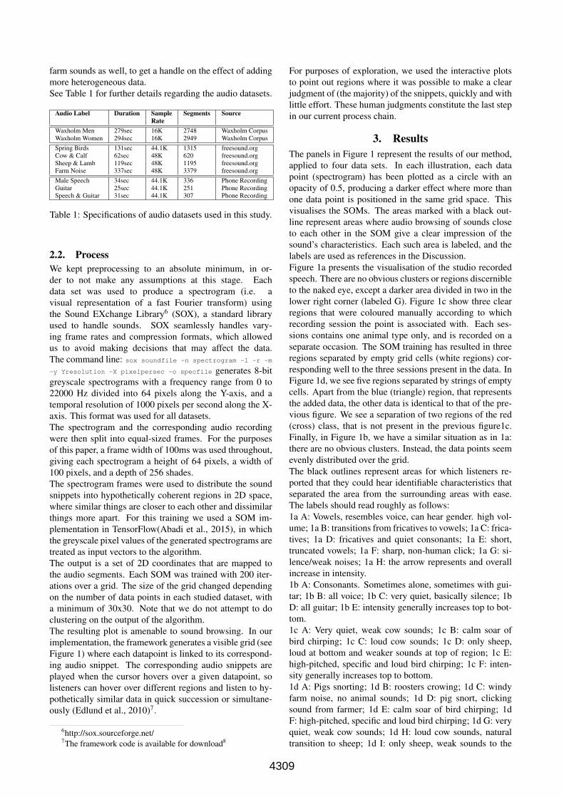
farm sounds as well, to get a handle on the effect of addingmore heterogeneous data.See Table 1 for further details regarding the audio datasets.

Audio Label Duration Sample Segments SourceRate

Waxholm Men 279sec 16K 2748 Waxholm CorpusWaxholm Women 294sec 16K 2949 Waxholm CorpusSpring Birds 131sec 44.1K 1315 freesound.orgCow & Calf 62sec 48K 620 freesound.orgSheep & Lamb 119sec 48K 1195 freesound.orgFarm Noise 337sec 48K 3379 freesound.orgMale Speech 34sec 44.1K 336 Phone RecordingGuitar 25sec 44.1K 251 Phone RecordingSpeech & Guitar 31sec 44.1K 307 Phone Recording

Table 1: Specifications of audio datasets used in this study.

2.2. ProcessWe kept preprocessing to an absolute minimum, in or-der to not make any assumptions at this stage. Eachdata set was used to produce a spectrogram (i.e. avisual representation of a fast Fourier transform) usingthe Sound EXchange Library6 (SOX), a standard libraryused to handle sounds. SOX seamlessly handles vary-ing frame rates and compression formats, which allowedus to avoid making decisions that may affect the data.The command line: sox soundfile -n spectrogram -l -r -m

-y Yresolution -X pixelpersec -o specfile generates 8-bitgreyscale spectrograms with a frequency range from 0 to22000 Hz divided into 64 pixels along the Y-axis, and atemporal resolution of 1000 pixels per second along the X-axis. This format was used for all datasets.The spectrogram and the corresponding audio recordingwere then split into equal-sized frames. For the purposesof this paper, a frame width of 100ms was used throughout,giving each spectrogram a height of 64 pixels, a width of100 pixels, and a depth of 256 shades.The spectrogram frames were used to distribute the soundsnippets into hypothetically coherent regions in 2D space,where similar things are closer to each other and dissimilarthings more apart. For this training we used a SOM im-plementation in TensorFlow(Abadi et al., 2015), in whichthe greyscale pixel values of the generated spectrograms aretreated as input vectors to the algorithm.The output is a set of 2D coordinates that are mapped tothe audio segments. Each SOM was trained with 200 iter-ations over a grid. The size of the grid changed dependingon the number of data points in each studied dataset, witha minimum of 30x30. Note that we do not attempt to doclustering on the output of the algorithm.The resulting plot is amenable to sound browsing. In ourimplementation, the framework generates a visible grid (seeFigure 1) where each datapoint is linked to its correspond-ing audio snippet. The corresponding audio snippets areplayed when the cursor hovers over a given datapoint, solisteners can hover over different regions and listen to hy-pothetically similar data in quick succession or simultane-ously (Edlund et al., 2010)7.

6http://sox.sourceforge.net/7The framework code is available for download8

For purposes of exploration, we used the interactive plotsto point out regions where it was possible to make a clearjudgment of (the majority) of the snippets, quickly and withlittle effort. These human judgments constitute the last stepin our current process chain.

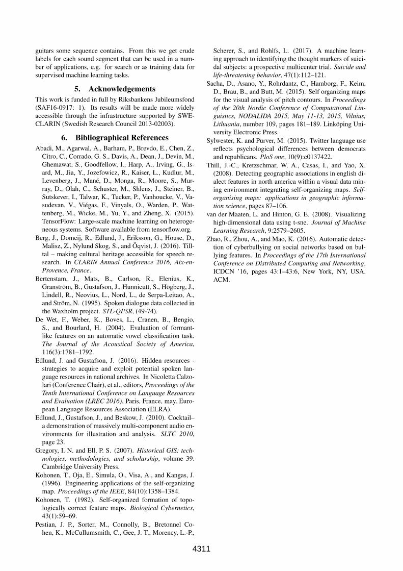
3. ResultsThe panels in Figure 1 represent the results of our method,applied to four data sets. In each illustration, each datapoint (spectrogram) has been plotted as a circle with anopacity of 0.5, producing a darker effect where more thanone data point is positioned in the same grid space. Thisvisualises the SOMs. The areas marked with a black out-line represent areas where audio browsing of sounds closeto each other in the SOM give a clear impression of thesound’s characteristics. Each such area is labeled, and thelabels are used as references in the Discussion.Figure 1a presents the visualisation of the studio recordedspeech. There are no obvious clusters or regions discernibleto the naked eye, except a darker area divided in two in thelower right corner (labeled G). Figure 1c show three clearregions that were coloured manually according to whichrecording session the point is associated with. Each ses-sions contains one animal type only, and is recorded on aseparate occasion. The SOM training has resulted in threeregions separated by empty grid cells (white regions) cor-responding well to the three sessions present in the data. InFigure 1d, we see five regions separated by strings of emptycells. Apart from the blue (triangle) region, that representsthe added data, the other data is identical to that of the pre-vious figure. We see a separation of two regions of the red(cross) class, that is not present in the previous figure1c.Finally, in Figure 1b, we have a similar situation as in 1a:there are no obvious clusters. Instead, the data points seemevenly distributed over the grid.The black outlines represent areas for which listeners re-ported that they could hear identifiable characteristics thatseparated the area from the surrounding areas with ease.The labels should read roughly as follows:1a A: Vowels, resembles voice, can hear gender. high vol-ume; 1a B: transitions from fricatives to vowels; 1a C: frica-tives; 1a D: fricatives and quiet consonants; 1a E: short,truncated vowels; 1a F: sharp, non-human click; 1a G: si-lence/weak noises; 1a H: the arrow represents and overallincrease in intensity.1b A: Consonants. Sometimes alone, sometimes with gui-tar; 1b B: all voice; 1b C: very quiet, basically silence; 1bD: all guitar; 1b E: intensity generally increases top to bot-tom.1c A: Very quiet, weak cow sounds; 1c B: calm soar ofbird chirping; 1c C: loud cow sounds; 1c D: only sheep,loud at bottom and weaker sounds at top of region; 1c E:high-pitched, specific and loud bird chirping; 1c F: inten-sity generally increases top to bottom.1d A: Pigs snorting; 1d B: roosters crowing; 1d C: windyfarm noise, no animal sounds; 1d D: pig snort, clickingsound from farmer; 1d E: calm soar of bird chirping; 1dF: high-pitched, specific and loud bird chirping; 1d G: veryquiet, weak cow sounds; 1d H: loud cow sounds, naturaltransition to sheep; 1d I: only sheep, weak sounds to the

4309

(a) Speech (76x76) (b) Guitar and voice (30x30)

(c) Animals (56x56) (d) Animals with farm noise (81x81)

Figure 1: SOMs based on different sound recordings. The colour-coded informationwas not visible to, nor derived from theprocess, but added manually for purposes of illustration: (red=birds; green=sheep; yellow=cows, blue=farm sounds). Thecircled and labeled areas represent manual selections of perceptually clearly similar sounds, based on audio browsing.

left and louder to the right; 1d J: loud cow sounds; 1d K:intensity generally increases left to right.

4. Discussion & future workAlthough we have only taken first steps towards combin-ing dimensionality reduction and visualisation techniqueswith novel audio browsing techniques, our first results arequite promising. For the speech only data in 1a, a listenercan quickly point out areas that are silent, that mainly con-tain vowels, and several other typical speech features. Thenext step here is to use the data in these relatively straight-forward areas to train models. The silence, for example,will let us model silence in the recording, which will makeit possible to segment the data on silence - something thatis not easily done in many recordings without spending aninordinate amount of time labeling silent segments sequen-tially and manually. The vowels may likewise be used totrain a vowel model, and separate vowels from other soundof high intensity. We may also find oddities: the tappingnoise in F turns out to be the press of a space bar, uponcloser inspection of the original data. It turns out that therecorded individuals were told to tap the space bar betweeneach utterance in this particular recording. For the gui-tar+voice data (1b), we quickly find vicinities with nothingbut voice and nothing but guitar. Again, this informationcan be used to create models or to inform a second clus-tering, effectively creating a reinforcement learning setup.For animals (1c and 1d), we see that sounds that differ in adistinct manner indeed end up further apart. At this stage,we cannot tell whether it is the recording conditions or theanimal noises, or both, that have the greatest influence, yetit is clear that the method we propose would work fairly

well to separate different (but unknown) datasets.

Our main goal in this work is to find a way into large setsof unknown data, and so far, we are encouraged by the re-sults. The strength of the proposed method lies in its abilityto generalise over different kinds of audio data. As such ithas an advantage in the context of large collections of founddata to methods that are restricted to only cover a particu-lar sound event. With that said, it should be noted that weare aware of many of the general improvements that canbe made to our process, but most if not all of them carrywith them a certain amount of assumptions about the data.For our purposes, we think it will be more fruitful to focuson developing the the audio browsing techniques first. Ournext step will be to create a more robust listening environ-ment. Listening to audio spatially distributed audio snip-pets is surprisingly efficient, but we must find out how lis-teners can best navigate to and point to different regions inthe soundscapes. With these methods in place, we can per-form full-scale tests on the perception of non-sequentiallystructured audio data. In the longer perspective, our goalis to add several possible last steps to the process chain.An obvious goal is to make the process iterative. The con-tinuous influx of rapidly acquired human judgments to thelearning process is highly interesting. More specific pro-cess chains are of equal interest. The silence modelingmentioned above is one such possibility. We are furtherinterested in taking the listener annotations, or judgments,and returning to the original sequential sounds. Simply la-beling the frames with their inverted distance (in 2D-space)to the centre of some human label and displaying that curveabove the diagonal sequential sound may be quite informa-tive, showing roughly how much speech, silence, cows, or

4310

guitars some sequence contains. From this we get crudelabels for each sound segment that can be used in a num-ber of applications, e.g. for search or as training data forsupervised machine learning tasks.

5. AcknowledgementsThis work is funded in full by Riksbankens Jubileumsfond(SAF16-0917: 1). Its results will be made more widelyaccessible through the infrastructure supported by SWE-CLARIN (Swedish Research Council 2013-02003).

6. Bibliographical ReferencesAbadi, M., Agarwal, A., Barham, P., Brevdo, E., Chen, Z.,

Citro, C., Corrado, G. S., Davis, A., Dean, J., Devin, M.,Ghemawat, S., Goodfellow, I., Harp, A., Irving, G., Is-ard, M., Jia, Y., Jozefowicz, R., Kaiser, L., Kudlur, M.,Levenberg, J., Mane, D., Monga, R., Moore, S., Mur-ray, D., Olah, C., Schuster, M., Shlens, J., Steiner, B.,Sutskever, I., Talwar, K., Tucker, P., Vanhoucke, V., Va-sudevan, V., Viegas, F., Vinyals, O., Warden, P., Wat-tenberg, M., Wicke, M., Yu, Y., and Zheng, X. (2015).TensorFlow: Large-scale machine learning on heteroge-neous systems. Software available from tensorflow.org.

Berg, J., Domeij, R., Edlund, J., Eriksson, G., House, D.,Malisz, Z., Nylund Skog, S., and Oqvist, J. (2016). Till-tal – making cultural heritage accessible for speech re-search. In CLARIN Annual Conference 2016, Aix-en-Provence, France.

Bertenstam, J., Mats, B., Carlson, R., Elenius, K.,Granstrom, B., Gustafson, J., Hunnicutt, S., Hogberg, J.,Lindell, R., Neovius, L., Nord, L., de Serpa-Leitao, A.,and Strom, N. (1995). Spoken dialogue data collected inthe Waxholm project. STL-QPSR, (49-74).

De Wet, F., Weber, K., Boves, L., Cranen, B., Bengio,S., and Bourlard, H. (2004). Evaluation of formant-like features on an automatic vowel classification task.The Journal of the Acoustical Society of America,116(3):1781–1792.

Edlund, J. and Gustafson, J. (2016). Hidden resources -strategies to acquire and exploit potential spoken lan-guage resources in national archives. In Nicoletta Calzo-lari (Conference Chair), et al., editors, Proceedings of theTenth International Conference on Language Resourcesand Evaluation (LREC 2016), Paris, France, may. Euro-pean Language Resources Association (ELRA).

Edlund, J., Gustafson, J., and Beskow, J. (2010). Cocktail–a demonstration of massively multi-component audio en-vironments for illustration and analysis. SLTC 2010,page 23.

Gregory, I. N. and Ell, P. S. (2007). Historical GIS: tech-nologies, methodologies, and scholarship, volume 39.Cambridge University Press.

Kohonen, T., Oja, E., Simula, O., Visa, A., and Kangas, J.(1996). Engineering applications of the self-organizingmap. Proceedings of the IEEE, 84(10):1358–1384.

Kohonen, T. (1982). Self-organized formation of topo-logically correct feature maps. Biological Cybernetics,43(1):59–69.

Pestian, J. P., Sorter, M., Connolly, B., Bretonnel Co-hen, K., McCullumsmith, C., Gee, J. T., Morency, L.-P.,

Scherer, S., and Rohlfs, L. (2017). A machine learn-ing approach to identifying the thought markers of suici-dal subjects: a prospective multicenter trial. Suicide andlife-threatening behavior, 47(1):112–121.

Sacha, D., Asano, Y., Rohrdantz, C., Hamborg, F., Keim,D., Brau, B., and Butt, M. (2015). Self organizing mapsfor the visual analysis of pitch contours. In Proceedingsof the 20th Nordic Conference of Computational Lin-guistics, NODALIDA 2015, May 11-13, 2015, Vilnius,Lithuania, number 109, pages 181–189. Linkoping Uni-versity Electronic Press.

Sylwester, K. and Purver, M. (2015). Twitter language usereflects psychological differences between democratsand republicans. PloS one, 10(9):e0137422.

Thill, J.-C., Kretzschmar, W. A., Casas, I., and Yao, X.(2008). Detecting geographic associations in english di-alect features in north america within a visual data min-ing environment integrating self-organizing maps. Self-organising maps: applications in geographic informa-tion science, pages 87–106.

van der Maaten, L. and Hinton, G. E. (2008). Visualizinghigh-dimensional data using t-sne. Journal of MachineLearning Research, 9:2579–2605.

Zhao, R., Zhou, A., and Mao, K. (2016). Automatic detec-tion of cyberbullying on social networks based on bul-lying features. In Proceedings of the 17th InternationalConference on Distributed Computing and Networking,ICDCN ’16, pages 43:1–43:6, New York, NY, USA.ACM.

4311