Bringing Fault Tolerance to

Hardware Managers in PESNet Yoon-Soo Lee

Thesis submitted to the faculty of the Virginia Polytechnic Institute and State

University in partial fulfillment of the requirements for the degree of

Master of Science

In

Computer Science and Application

Stephen Edwards, Chair

James Arthur

Shawn Bohner

July 26, 2006

Blacksburg, Virginia

Keywords: Network, Protocol, PEBB, PESNet, Fault Tolerance

Bringing Fault Tolerance to

Hardware Managers in PESNet

Yoon-Soo Lee

(ABSTRACT)

The goal of this research is to improve the communications protocol for Dual Ring Power

Electronics Systems called PESNet. The thesis will focus on making the protocol operate in a more

reliable manner by tolerating Hardware Manager failures and allowing failover among duplicate

Hardware Managers within PEBB-based systems. In order to make this possible, two new features

must be added to PESNet: utilization of the secondary ring for fault-tolerant communication, and

dynamic reconfiguration of the network. Many ideas for supporting fault tolerance have been

discussed in previous work and the hardware for PEBB-based systems was designed so support fault

tolerance. However, in spite of the capabilities of the hardware, fault tolerance is not supported yet by

existing firmware or software. Improving the PESNet protocol to tolerate Hardware Manager failures

will increase the reliability of power electronics systems. Moreover, the additional features that are

needed to perform failover also allow recovery from link failures and make hot-swap or plug-and-

play of PEBBs possible. Since power electronics systems are real-time systems, it is critical that

packets be delivered as soon as possible to their destination. The network latency will limit the

granularity of time that the control application can operate on. As a result, methods to implement the

required features to meet real-time system requirements are discussed and changes to the protocol are

proposed. Changing PESNet will provide reliability gains, depending on the reliability of the

components that are used to construct the system.

iii

Table of Contents

Chapter 1: Introduction ....................................................................................................................... 1 1.1 Introduction to Power Electronics Building Blocks................................................................. 1

1.1.1 Motivation of Power Electronics Building Blocks ........................................................ 1 1.1.2 Power Electronics Building Blocks (PEBBs) ................................................................ 2

1.2 PESNet..................................................................................................................................... 3 1.2.1 PESNet 1.2..................................................................................................................... 3 1.2.2 PESNet 2.2 (DRPESNet)............................................................................................... 6 1.2.3 Problems in PESNet ...................................................................................................... 9

1.3 Problem Statement ................................................................................................................. 11 Chapter 2: Related Work................................................................................................................... 14

2.1 Fiber Distributed Data Interface (FDDI) ............................................................................... 14 2.2 Various Dual Ring Topologies ............................................................................................... 17 2.3 Failover in other Protocols..................................................................................................... 19

2.3.1 Passive Replication Methods....................................................................................... 20 2.3.2 Active Replication Methods......................................................................................... 20

Chapter 3: Utilizing the Secondary Ring .......................................................................................... 22 3.1 Fault Detection, Recovery, and Healing ................................................................................ 22 3.2 Preventing Packet Loss .......................................................................................................... 26 3.3 Reducing Network Delay during Failure Mode..................................................................... 27

Chapter 4: Silent Failover ................................................................................................................... 30 4.1 Requirements for the Failover Process in PEBB ................................................................... 30 4.2 Adopting Existing Failover Techniques ................................................................................. 31

4.2.1 Using Passive Replication ........................................................................................... 32 4.2.2 Using Active Replication............................................................................................. 34

4.3 Silent Failover through Multicast using Active Replication .................................................. 36 Chapter 5: Dynamic Reconfiguration ............................................................................................... 42

5.1 Dynamic Network Reconfiguration in PESNet 2.2 ............................................................... 42 5.2 Modifications to PESNet 2.2 ................................................................................................. 44

5.2.1 Application Manager Implementation ......................................................................... 44 5.2.2 Hardware Manager Implementation ............................................................................ 46

Chapter 6: Changes to PESNet and Implementation........................................................................... 48 6.1 Packet Structure of PESNet 2.2 ............................................................................................. 48 6.2 Required Changes to the Packet Structure ............................................................................. 49

iv

6.2.1 Changes Related to Utilization of the Secondary Ring ............................................... 49 6.2.2 Changes Related to Silent Failover.............................................................................. 51 6.2.3 Changes Related to Dynamic Reconfiguration............................................................ 51

6.3 Overall Changes to PESNet Packet Structure........................................................................ 51 Chapter 7: Analysis of the Protocol .................................................................................................. 54

7.1 Maximum Switching Frequency............................................................................................ 54 7.2 System Reliability with PESNet ............................................................................................ 57

Chapter 8: Conclusion....................................................................................................................... 64 8.1 Summary ................................................................................................................................ 64

8.1.2 Utilizing the Secondary Ring....................................................................................... 64 8.1.3 Silent Failover.............................................................................................................. 65 8.1.4 Dynamic Reconfiguration............................................................................................ 66 8.1.5 Overall Summary......................................................................................................... 67

8.2 Remaining Problems and Future Work .................................................................................. 67 8.3 Closing Remarks.................................................................................................................... 68

References ........................................................................................................................................... 70 Appendix............................................................................................................................................. 72

A-I PESNet Simulator.................................................................................................................. 72 A-I-a Simulator Assumptions ............................................................................................... 72 A-I-b Simulator Implementation .......................................................................................... 73

v

List of Figures

Figure 1: Single Ring Topology ............................................................................................................ 4 Figure 2: Counter Rotating Dual Ring Daisy Chained Topology ......................................................... 7 Figure 3: Use of Secondary Ring with Faults ....................................................................................... 8 Figure 4: Flexible Network Topology in FDDI................................................................................... 16 Figure 5: Double Loop (Dual Ring) Topology.................................................................................... 18 Figure 6: Daisy Chained Loop Topology ............................................................................................ 18 Figure 7: Optimal Loop Topology with 15 Nodes, Skip distance 3 .................................................... 19 Figure 8: Ring-wrap operation upon fault detection ........................................................................... 23 Figure 9: Forwarding Mechanism....................................................................................................... 24 Figure 10: Application Manager State Diagram.................................................................................. 45 Figure 11: Hardware Manager State Diagram..................................................................................... 47 Figure 12: Switching Cycle for Different Number of Nodes and Operating Mode ............................ 56 Figure 13: Gained Reliability.............................................................................................................. 61 Figure 14: Simulator Class Diagram................................................................................................... 73 Figure 15: Snapshot of the implemented Simulator............................................................................ 75

vi

List of Tables

Table 1: PESNet 2.2 Packet Structure and Description....................................................................... 49 Table 2: New Packet Structure for PESNet......................................................................................... 52 Table 3: Actual Reliability of System Using PESNet ......................................................................... 62

1

Chapter 1: Introduction This thesis introduces a reliable network protocol for the Power Electronics Building Blocks

(PEBB) architecture, which is a modular approach to power electronics systems [1]. Power

electronics systems convert power from one form to another. Hence, they are also known as power

conversion systems. This chapter is an introduction to the PEBB approach for power electronics

applications. The motivation of the PEBB approach is explained first. Background knowledge about

the PEBB architecture that is needed to understand this thesis will follow. Based on the introduction,

the problems in the current version of PESNet are specified. This chapter closes by laying out the

problem to be addressed.

1.1 Introduction to Power Electronics Building Blocks 1.1.1 Motivation of Power Electronics Building Blocks

Traditional digitally controlled power electronics systems were designed in a centralized manner

[2, 3]. The centralized systems lacked flexibility in their designs. Lacking flexibility in the designs

has led to long development cycles. Furthermore, maintenance of the control software requires a lot

of effort. Debugging the control software of such a system is difficult because of the lack of

standardization and modularization, and the tight dependence on the system hardware [4]. Moreover,

the lack of flexibility in constructing the system limits the reliability that can be achieved. As

application of power electronics systems is spread widely in many areas, use of the system in medical

equipment and electrical vehicles require high level of reliability. Ways to reduce the development

cycle, reduce the maintenance cost, reduce the manufacturing cost, and increase reliability have been

an active research topic in the field of power electronics.

Attempts to modularize power electronic systems into commonly used parts have been made to

increase flexibility and reliability. With the existence of commonly used modules, engineers hoped

that development cycles can be reduced by being able to integrate existing modules. Also, the

manufacturing cost was expected to decrease if the modules were produced in great volume.

2

However, power electronics systems that control and manage power stages in a centralized manner

have many drawbacks. The variety of signals transmitted through different physical media in

centralized designs makes it difficult to standardize and modularize. Therefore, a different approach

was needed to modularize such systems [5].

1.1.2 Power Electronics Building Blocks (PEBBs) Modularization issues similar to those in power electronics systems also have been addressed in

the field of computer science. In the early years of computer software, the development cycle of

software became longer as the scale of the software that was being written grew. As the size of

software started to grow, the complexity of the control structure of the software also became

unmanageable. As a result, not only did development take longer, but maintenance of the software

also became more time consuming. These problems caused the Software Crisis which emerged in the

late 1960’s. Consequently, efforts to increase the flexibility of constructing software have been made

by software engineers. As a result, techniques such as Object-Oriented programming were developed

to modularize software. Modularization of software made reuse of software modules possible.

The concept of a PEBB takes a similar approach to the one that has already been applied to

software. Computer software concepts and technologies have been applied to power electronics

applications to increase flexibility and reusability of power electronics systems. The primary goal of

the PEBB architecture is to provide an environment for developing decentralized power electronics

systems. PEBBs are standardized power electronics components that can be used to integrate power

electronics systems [4, 6]. The PEBB architecture uses an open, distributed control approach that was

proposed for constructing low-cost, highly reliable power electronics systems by interconnecting

PEBBs [5].

In general, the task of controlling a power electronics system can be abstracted into two different

tasks. One task is to follow the converter control algorithm and the other is to interface with system

hardware [7]. Therefore a PEBB can fall into two categories. A PEBB can be either a power

processing unit or the main controller. A PEBB that is responsible for carrying out the converter

control algorithm is called an Application Manager. A PEBB that provides an interface with the

hardware is called a Hardware Manager [4].

3

As a result of modularizing the control structure of power electronics systems, communication

among the modules (PEBBs) is required. Therefore, communication links are introduced in the

distributed controller architecture. The term “open” indicates the flexibility and adaptability that the

system can achieve by interconnecting the PEBBs via a network. The architecture suggests that

PEBBs be interconnected via high-speed communication links and interoperate in a decentralized

manner because of the massive amount of data that must be transferred among the PEBBs [8, 9].

Because of resource utilization and synchronization issues, a dual ring network topology was chosen

[10]. The advantages that these topologies bring are reduction in cost and more sophisticated use of

transmission media. In order for the PEBBs to communicate in this kind of network environment, a

protocol called PESNet has been developed [4, 7, 11-13].

Modular approaches to power electronics systems have introduced a flexible method of

construction that also brings the potential for increased reliability. Modular design also introduces the

possibility of adding redundant modules in the system when needed. However, reliability of the

system was brought to attention again as communications links are added to the system. The network

may not be as reliable as desired, since optical fiber links are vulnerable to heat and may not function

properly when bent. Therefore, methods to improve the reliability of the network are needed. The

ability to add redundant modules dynamically and to make the network tolerant to communications

link failure can be solved by enhancing the PESNet communications protocol.

1.2 PESNet

PESNet was developed as a protocol to support communications between PEBB nodes (the term

node will refer to a PEBB from this point on unless specified otherwise) connected with optical fiber

communications links using a ring topology. PESNet has gone through a major change after its initial

version. However, some important ideas and basic behavior of the network driven by the protocol

were specified in the first version and remained the same in later versions. For this reason, this

section will introduce PESNet by examining its two major versions.

1.2.1 PESNet 1.2 Since optical fiber links are unidirectional, communication between nodes occur in one direction.

4

Each node contains one transmitter and a receiver. Therefore, the network is constructed by

connecting one node’s transmitter to another node’s receiver, as shown in Figure 1.

Figure 1: Single Ring Topology

An important characteristic of the network behavior of the PESNet protocol compared to other

existing network protocols is that a packet visits every node that is between the source node and the

destination node. Unlike other network protocols, a packet may not bypass a node as it propagates to

its destination node. Instead, all nodes receive and send packets simultaneously. Therefore, the

network must be synchronized. At each synchronized period, a check is performed to determine

whether a received packet is destined for the current node. If the packet is not destined for the current

node, the node will forward the packet to the next node at the following network synchronization step.

For synchronization purposes, there must always be a packet sent between neighboring nodes. An

NS_NULL packet, which does not contain any meaningful data, will be sent to the next node when

there is no meaningful packet to be sent to the neighboring node for this reason. As mentioned in Section 1.1.2, PEBBs fall into two categories. A power electronics system that

consists of PEBBs will have at least one Application Manager node and at least one Hardware

Manager node. The system operates in a Master-Slave fashion where Application Managers send

commands to Hardware Managers and Hardware Managers respond to the commands issued from

the Application Managers. Obviously, the Application Managers correspond to the masters and the

Hardware Managers correspond to the slaves. A command from an Application Manager can be

either a command retrieving some data from a Hardware Manager, or a command requesting a

Hardware Manager to carry out a specific action. The quality of the protocol depends on how quickly

it can deliver the requests and responses. A power electronics application is generally driven by the

Application Manager by requesting data and issuing commands at a certain frequency, which we call

the switching frequency. If the switching frequency increases, the application is able to control the

5

power electronics system more precisely and allows the system to generate higher quality output.

Therefore, the frequency that an Application Manager can operate at becomes an important property

of PESNet.

In order to implement the Master-Slave type of communication behavior, two types of packets are

defined in the PESNet protocol: data packets and synchronization packets. Both types of packets

have a common field that indicates the address of the destination node. A data packet contains a 4-

byte field containing the data that is to be transferred to another node. In power electronics systems,

it is important that some actions are carried out in a synchronized manner. A synchronization packet

is used for synchronizing actions performed across multiple Hardware Managers. A synchronization

packet contains the information about the action that is to be carried out. There is no specific field

that directly relates to the synchronization. Instead, the synchronization is done with the advantages

of network behavior. As explained earlier in this section, the transmission and reception of packets on

the network is synchronized. Using this property of the network, the Application Manager

synchronizes Hardware Managers by sending out synchronization packets in the order of packets that

are destined from the farthest to the closest to the Application Manager in the direction of the packet

flow. As a result, all Hardware Managers receive their corresponding synchronization packet at the

same time.

There are some major drawbacks to this version of the PESNet protocol. First of all, the protocol

lacks reliability. The network topology that the protocol operates upon is sensitive to failures. The

network will fail if any individual link or any individual node fails because of the use of a single ring

topology with unidirectional communication links. Since both communication links and nodes play

an important role in the network, not even a single point of link failure or a single physical node

failure can be tolerated. Any failure will destroy the closed loop ring configuration of the network

and packets will not be able to be transferred between the nodes separated by the point where the

failure has occurred. Secondly, the protocol lacks flexibility. The flexibility issue has much to do with

synchronization of Hardware Managers. The synchronization approach among Hardware Managers

that is taken from this protocol requires that the Application Manager has precise knowledge of the

network topology, since the process depends on the exact ordering of the connected nodes. As a

result, the configuration of the Application Manager must be changed dynamically if a new node is

introduced in the network. However, no dynamic reconfiguration scheme for the Application

Manager is present in the protocol. This implies that no new nodes can be added to or removed from

the network during operation. Also, because the location and address of every Hardware Manager

6

must be hard-coded into the Application Manager, all the information about the nodes and the

ordering of the connections must be known prior to operation.

1.2.2 PESNet 2.2 (DRPESNet)

Changes were made to PESNet 1.2 to address some of its shortcomings, resulting in PESNet 2.2.

The goal for PESNet 2.2 was to extend the protocol to provide reliability to the PEBB architecture.

The following are the requirements of PESNet 2.2:

� Use of secondary ring

� Improved synchronization

� Support for multiple masters (Application Managers)

The most significant change that was suggested in PESNet 2.2 is the network topology that the

protocol operates on. In order to tolerate link failure and physical node failure to some extent, the

topology of the network has been revised to have redundant communications links. The idea was

borrowed from the Fiber Distributed Data Interface (FDDI) protocol. Obviously, redundant network

resources increase reliability. A new ring was added to the original network topology that the

architecture used and research has been done to find an effective way to use the redundant network

resource for increasing reliability.

Similar to FDDI, PESNet 2.2 uses a counter-rotating dual-ring topology. The intent was to utilize

both rings when communicating to make the network fault tolerant. The difference from the single

ring topology is that there exist two rings where communication flows in opposite directions.

Therefore, a PEBB has two sets of transmitters and receivers. Neighboring nodes are connected by

connecting two optical fiber links, each connected from the transmitter of one node to the receiver of

the other. The topology of the network is shown in Figure 2. By having two counter-rotating rings,

the network will be able to tolerate one or more points of failure in the network depending on the

location of the failure in the ring. The reason for having counter-rotating rings is for tolerating node

failures. Only link failures could be tolerated if both rings were operating in the same direction.

7

Figure 2: Counter Rotating Dual Ring Daisy Chained Topology

Although another network ring is introduced, only one ring, which is denoted as the primary ring,

is used for communication when there are no faulty links or nodes. When the primary ring itself is

used for communication, we say that network is in normal operation mode. The other ring, which

we denote as the secondary ring, is only used in case of faults. The presence of another ring that

operates in the opposite direction from the primary ring makes it possible for the network to provide

an alternative path for communication between nodes when a link or node fails. The operation of

isolating the failed link or node and forwarding packets to the alternative path provided by the

secondary ring is known as the ring-wrap operation in FDDI. The nodes adjacent to the point of

failure make adjustments to the packet forwarding pattern. The node that is located before and after

the point of failure in the down stream will each start forwarding packets to the other ring.

The packets that are routed to the secondary ring are always forwarded to the neighboring node on

the secondary ring until it has reached the other side of the point of failure without exception.

Therefore, a node that receives a packet on the secondary ring that is addressed to itself will not

consume it, but rather forward it to the next node on the secondary ring. Since no packets are

consumed on the secondary ring, the destination of a packet is not required to be examined when

received on the secondary ring. Therefore, the fault is transparent to all the nodes except the nodes

that reside at both ends of the point where the failure occurred and that must perform the ring-wrap

operation. In the big picture, the packet flow will be observed as if a packet is magically sent through

the faulty part of the primary ring. However, a large delay will exist when a packet is sent from one

end of the point of failure to the other end of the point of failure. When the packets are routed to the

secondary ring due to a failure, we say that the network is operating in failure mode. Figure 3

explains the network behavior during failure mode. Once point of failure has recovered, there is a

transition from failure mode back to normal mode. We say that the network is in recovery mode

8

during this transition.

Figure 3: Use of Secondary Ring with Faults

The Hardware Manager synchronization scheme was changed in a way so that the process does not

depend on the physical configuration of the network. In order to achieve this, the concept of a Global

Network Clock has been developed. As mentioned in the previous section, the network operates in a

synchronized manner. The Global Network Clock takes advantage of the fact that transmission and

reception of packets are synchronized at all the nodes. All the nodes in the network synchronize their

Global Network Clock according to the network synchronization. After each network

synchronization, each node increments their Global Network Clock. Because the Global Network

Clock is synchronized, nodes have an agreement on time. As a result, synchronization commands can

be sent from the Application Manager based on the Global Network Time that the Global Network

Clock indicates. The synchronization packet was changed so that the content of the synchronization

packet contains the Global Network time at which a command is to take effect. This feature has

already been implemented in the version 2.2 of PESNet.

Although version 2.2 of PESNet was designed with the intent of allowing multiple masters

(Application Managers), this version of the protocol only supports a single master at the moment.

However, multiple masters may be desired. The benefit of having multiple masters is the ability to

distribute the control algorithm across multiple processors. The workload for each master may

decrease significantly by distributing the control algorithm to multiple masters, making it possible to

9

use more complex control algorithms that require more resources. Moreover, given the fact that

PEBB power electronics applications require at least one master, even when an application does not

require multiple masters it can benefit from having multiple masters to increase reliability through

redundancy. However, the reason for having the single master constraint is for simplicity. In addition

to this constraint, the complete configuration of the entire network must be known prior to operation

at the moment. The ordering of the connected nodes in the network and their addresses must be hard

coded in the master for the network to operate. This constraint limits the flexibility and reliability that

can be achieved throughout constructing and maintaining the network. Since the network

configuration is hard coded in the master, the network configuration cannot be changed during

operation. Improvements such as assigning network addresses to the nodes in the order they are

connected after the master in the primary ring have been proposed. But this approach introduces

another limitation. In the case of multiple masters, one must be designated to allocate addresses.

When the designated master fails, it becomes impossible to add new nodes because a network

address will never be assigned to it. A more flexible scheme for the masters to learn the configuration

of the network dynamically and assign network addresses to new nodes dynamically is necessary to

increase flexibility. At the same time, support for multiple masters is desired to increase reliability of

the system and allow for distributed control algorithms.

1.2.3 Problems in PESNet

The most significant change to PESNet in version 2.2 is the network topology. Use of a counter-

rotating dual ring topology was expected to increase the reliability of the network. However,

although others [12, 13] have described how to utilize the secondary ring and provided development

direction, proper use of the secondary ring to tolerate faults was not implemented in PESNet 2.2.

There may be many reasons for the slow maturation of the protocol. While previous work shows the

basic concept of using the secondary ring, more analysis of the requirements for taking advantage of

the topology was needed. The following are the requirements that must be satisfied in order to make

the network fault tolerant by taking advantage of the counter-rotating dual ring topology:

� Support for duplicate slaves (Hardware Managers) and failover among duplicate nodes

� Support for dynamic network reconfiguration

Network behavior specified for utilizing the secondary ring in previous work is meaningless

10

without these requirements. Previous work neglects the fact that the system can fail when a node fails.

The specified network behavior may tolerate link failures, but it cannot tolerate node failures. For

example, assume there is a system that requires some number of nodes that have different

responsibilities in the system to communicate in order to operate. The system will continue to operate

when a link failure occurs since all the nodes are able to carry out their responsibilities. However,

suppose a node fails. All nodes beside the failed node will be able to communicate and operate.

However, the failed node will not be able to carry out its responsibilities in the system. Hence, the

system will fail. Therefore, just as it is desirable to have multiple masters, it is also desirable to

support duplicate Hardware Managers. The term “duplicate” indicates the presence of multiple

Hardware Managers that carries out identical tasks—redundant or “spare” PEBBs that can take over

when their primary counterpart fails. Having duplicate Hardware Managers allows greater reliability

through redundancy. A set of redundant Hardware Managers that replicates a certain Hardware

Manager in the system will allow one of the replicas to fail without having to halt the system. When

there are duplicate Hardware Managers, the system can perform a failover when there is a node

failure. The duplicate Hardware Manager that takes over for the failed node is acting as a hot spare.

This feature will allow the system to operate normally in spite of losing a node from failing.

Another desirable capability of the protocol is to allow Hot-Swap and Plug-and-Play. Hot-swap is

the ability to remove or replace a component in the system during operation without affecting the

system’s operation—in other words, without requiring it to shut down and restart. Plug-and-play is

the ability to introduce new nodes in the network during system operation. By allowing Hot-Swap

and Plug-and-Play, system maintainers will be able to replace faulty nodes or remove nodes for

whatever reason and add new nodes without halting the system. While the current protocol does not

support these features, adding these capabilities can increase flexibility in constructing and

maintaining the system. Also, the reliability of the system can increase as adding a duplicate node

becomes trivial. Support for hot-swapping and plug-and-play is needed not only to provide flexibility

in constructing and maintaining the system, but also to provide a mechanism for the system to heal

while the system is operating. The situation of a node failing due to a temporary power failure is

similar to a situation where a node is disconnected and reconnected to the network. When a node

physically fails temporarily and is able to recover by itself, the network can return back to normal

operation.

However, support for dynamic reconfiguration of the network is needed to make hot-swap and

plug-and-play possible. The need for dynamic reconfiguration of the network arises in two situations.

11

One situation is when the system has just started. The other is when the network configuration has

changed because a new node was added. When a node recovers from a failure, it may have lost its

network configuration parameters such as its address. Therefore, the recovered node can be treated

the same as a newly introduced node, requiring the network to reconfigure. Also, considering the fact

that the primary ring must be broken in order to add a new node on the network, use of the secondary

ring to maintain communications integrity during the transition is essential.

Implementing a fault tolerant network by utilizing the secondary ring may have been difficult

because of insufficient requirements analysis in prior work. The two additional requirements above

were briefly stated by previous researchers, but they were considered as independent issues rather

than steps that must be taken in order to implement a fault tolerant network. The complexity of the

relationship between the requirements for PESNet and the problems might have made the analysis

difficult. Also, there remain unanswered questions for implementation. For instance, the network

behavior of PESNet 2.2 on the new network topology has been specified vaguely without the

discussion of detecting faults and the forwarding mechanism used during healing mode. Another

reason may be because of the effort to keep the protocol simple enough to implement the basic

features easily.

1.3 Problem Statement

This thesis concentrates on adding features to make PESNet reliable by allowing the network to

employ redundant resources. In addition to supporting the secondary ring with redundant links, this

work enables transparent failover among duplicate Hardware Managers, resulting in increased

reliability of power electronics systems. Since the thesis is focused on failover among duplicate

Hardware Managers, allowing multiple masters will not be considered as a requirement for reaching

our goal. Also, since hot-swap and plug-and-play both require utilization of the secondary ring and

dynamic reconfiguration of the network, the problem of implementing failover among Hardware

Managers can be summarized by three requirements:

� Making use of the secondary ring in presence of node and link failure.

� Allowing duplicate Hardware Managers for failover.

� Supporting dynamic reconfiguration of the network.

12

The additional features will not only allow failover among Hardware Managers but also allow hot-

swap and plug-and-play operation, which we expect to increase the reliability of power electronics

applications as it can tolerate faults that occur during runtime. The three requirements will be

approaches as follows:

� Utilizing the secondary ring: There are three problems in achieving this goal. First, the current

version of PESNet lacks the ability to detect and report faults in the network. Although PEBBs

were initially designed to handle faults, no documents about detecting faults have been found.

Second, previous studies have concentrated on the transition from normal operation mode to

failure mode. However, there are unanswered questions about the network behavior during

healing mode. Third, the network path through the secondary ring during failure mode introduces

a large network delay compared to normal mode. A large network delay may limit the granularity

of the time interval used for controlling the system. A method to detect faults in the network and a

proper scheme to reroute the packets to the primary ring after the primary ring has recovered at

the point of failure must be specified. Also, it is desirable to decrease the network delay when

using the secondary ring by using a slightly modified network topology.

� Allow duplicate Hardware Managers for failover: The current protocol, which operates in a

master slave style of communication where control of the application is centered at the master, has

drawbacks in supporting failover among hot spares. When control of the application is the master

node’s responsibility, the failover process cannot be completed when the master node fails.

Moreover, the failover process in the master-slave type communication requires a long process.

Because of limits imposed by the network topology, it is impossible to shorten the failover

process in the master-slave type of communication. A distributed failover approach among

Hardware Managers is proposed in order to make the failover process transparent to the master

and to reduce the time of the process.

� Dynamic network reconfiguration: Currently, all network address assignments and the physical

configuration of the network (ordering of the connected nodes) must be hard-coded into the

master Application Manager. This approach is completely static. Although, a dynamic way of

configuring the network has been proposed, it can be improved further to increase flexibility. The

major issue in dynamic reconfiguration is issuing network addresses to nodes and dynamically

configuring them while the network is in operation. The process of assigning addresses

13

dynamically when there are multiple masters—that is, multiple Application Manager nodes to

support distributed control algorithms—must be solved.

The augmentation of the protocol will be based on prior work for consistency of the PEBB project.

14

Chapter 2: Related Work

This chapter contains information about prior work that relates to solving the problem addressed

by this thesis. PESNet works in a very unique way and not much previous work relates to it directly.

Even though PESNet borrows many ideas from FDDI, it is different in many ways. Hence, the

research discussed here may not provide direct solutions, but rather gives a better understanding of

the problems that exist in PESNet. Related work can be categorized into three primary areas:

� Fiber Distributed Data Interface (FDDI)

� Various dual ring topology networks

� Failover in other protocols

For the work that is discussed in the following subsections, the ideas that potentially can be

adopted in PESNet or that may help explain its problems will be emphasized by comparison with the

work in this thesis.

2.1 Fiber Distributed Data Interface (FDDI)

Here we examine the Fiber Distributed Data Interface (FDDI) protocol [14]. The protocol has

many derivations such as FDDI-II or FBRN, but we only take a look at the simplest version since it

is most similar to the PESNet protocol. FDDI is a standardized dual ring protocol based on the token

ring model. It was developed to operate on a 100Mbit/s local area network (LAN) using optical

fiber as the medium. Many of the physical characteristics are similar to PESNet 2.2. However, there

are some differences that are worth mentioning.

First, unlike PESNet, FDDI is a timed-token protocol. The physical layer of FDDI behaves exactly

the same as the PESNet physical layer. All the nodes receive and transmit simultaneously at the

physical layer. However, at the network layer, only the node that holds the token is able to initiate a

data transmission. After a node has possession of the token for a certain amount of time, the token is

15

passed to the next node. The reason for discarding the token ring medium access scheme in PESNet

is to increase spatial utilization of network resources. Spatial reuse of bandwidth allows efficient use

of the network and increases throughput [15]. While only one node is able to transmit data into the

ring at any given time for a token ring protocol, spatial reuse of bandwidth allows concurrent data

transmission from multiple nodes. The idea was to allow concurrent data transmission at multiple

nodes where different portions of the rings can be used simultaneously. The disadvantage of

incorporating spatial reuse of the ring is the possibility of starvation. If some node is constantly

involved in providing network bandwidth between two nodes, that node will not be able to transmit

its own data on the ring until the other two allow the opportunity. As a result, a fairness algorithm

must be present to avoid the starvation phenomenon. In PESNet, a different approach was taken to

prevent starvation. The network layer is designed to synchronize with the physical layer of the

protocol. As a result, all the nodes receive and transmit data packets simultaneously, as explained in

Section 1.2. This method provides an environment where all nodes can transmit data packets as

needed. Because of this network behavior, while FDDI strictly follows the seven layers of the Open

System Interconnection (OSI) reference model, PESNet only has three layers. The communications

protocol layer was reduced to three layers to decrease the overhead required at each node when

receiving and transmitting data packets.

Second, there are various options for constructing the network topology. In FDDI, there are four

types of devices that can be attached to the network: single attached stations, dual attached stations,

single attached concentrators, and dual attached concentrators. The device called a concentrator

increases the flexibility of creating the network topology. The dual ring can be constructed from dual

attached devices such as dual attached stations and dual attached concentrators. More devices can be

attached to the concentrators. The devices that are attached to concentrators can be in a tree structure,

as shown in Figure 4.

16

Figure 4: Flexible Network Topology in FDDI

Third, there is a difference in the method of providing fault tolerance to the network. The ring-

wrap operation in FDDI works as the same as in PESNet. In fact, PESNet’s ring-wrapping idea was

inspired by FDDI. However, there is another way of tolerating faults in FDDI by using concentrators.

The concentrators are equipped with the capability of bypassing incoming data to the next node. To

be precise, the data being received via optical signal is directly sent to the next node. The bypass

switch can be configured to turn on automatically or manually. Instead of performing a ring-wrap

operation when a node that is connected to a concentrator has physically failed or is powered down,

the concentrator can perform a signal bypass. The signal bypassing capability of concentrators makes

it possible to maintain the integrity of the primary ring in spite of multiple node failures by isolating

them from the ring. Failure of nodes that are connected to concentrators can be tolerated without the

network delay that would have been caused by the ring-wrapping operation.

The fault detection and recovery process in PESNet can become complicated due to many reasons.

The additional communications links for redundancy introduce various scenarios of network failure

and each scenario must be handled appropriately. The difficulty of detecting and recovering from

faults come from the fact that faults can only be detected on the receiving side of a communications

link. This characteristic makes it difficult to detect faults that occur at the next node downstream.

This limitation makes it difficult to initiate a ring-wrap operation at appropriate situations. Also, each

node does not have the ability to determine whether the fault is caused by a node failure or a link

failure. The nodes detect faults by examining signals they receive. However, a weak signal or no

signal being received can be caused by either a link failure or a node failure.

Since PESNet is based on FDDI, it is worthwhile to examine the fault detection and recovery

process in FDDI. The fault detection and recovery process of FDDI follows the IEEE 802.5 standard

17

for the token ring protocol (IEEE 802.5-1989). Because this thesis focuses on physical failure, the

term fault refers to a physical node failure or link failure here. Such faults influence the network’s

operation, unlike logical failures that do not have any impact on the network’s behavior. Therefore,

the discussion of packet loss in the network due to data corruption is neglected in this thesis, which

concentrates on detecting physical failures.

Although the network can operate normally in spite of failures that occur on the secondary ring if

the primary ring remains intact, the failure that occurs on the secondary ring is as critical as a failure

that occurs on the primary ring. The reason is because a link failure on the secondary ring affects the

network’s ability to recover when another link failure on the primary ring is introduced at another

link pair. Therefore, a link failure is treated as if the pair of opposing links connecting two nodes—

one on the primary ring and one on the secondary ring—have both failed. The illusion of a pair of

links failing after one of the link has failed is achieved by forcing the other link of the pair to stop

transmitting. This enables the two nodes at either end of the point of failure to detect the failure at the

same time. After a fault is detected, beaconing starts to initiate the ring-wrap operation. However,

beaconing to carry out the ring-wrap operation in FDDI requires the nodes to communicate

excessively and induces a long transition time.

2.2 Various Dual Ring Topologies

The throughput of PESNet is greater than FDDI because of spatial reuse of bandwidth. While real-

time applications can benefit from the increased throughput, there may also be long delays when the

secondary ring is in use. If we define the unit of delay in hops, which is the number of links that the

network packet has to propagate through to reach its destination node, we can see that an additional

n-1 hops are needed when there is a faulty link between the two communicating nodes, and an

additional n-2 hops are needed when there is a faulty node. The delay of the network is limited by the

physical structure of the topology. Therefore, to reduce the network delay the topology must change.

Ideas for finding optimal topologies for dual ring networks for distributed systems [16] are

introduced in this section. The ideas discussed here use both rings for communication all the time,

unlike the PESNet approach of using only the primary ring for communication during normal

operation. Even though PESNet utilizes the secondary ring when a fault is present in the network, it

is different from using both rings for communication since the packets cannot be accepted from the

18

secondary ring from the nodes.

Initially, the dual ring network emerged to support fault tolerance [16]. The topology remained

simple, with two counter-rotating rings as shown in Figure 5. Suppose there are n nodes in the ring

and all components are operating normally. If both counter-rotating rings are used for sending and

receiving messages, the average number of hops for communication between two nodes is reduced to

n/4, while the average number of hops for a single ring network is n/2. In the presence of a fault, the

average number of hops becomes n/2 while the single ring cannot tolerate any faults in the network.

Figure 5: Double Loop (Dual Ring) Topology

Later, a daisy-chained topology was proposed to reduce the required hops in communication [16].

The daisy-chained topology is slightly more complicated than the simple dual-ring topology. While

one ring, the forward loop, is constructed by interconnected neighboring nodes, the other loop is

constructed by interconnecting nodes that are h nodes apart, as shown in Figure 6. The number h

which is denoted as the skip distance is 2 in Figure 6.

Figure 6: Daisy Chained Loop Topology

19

While there is no specific value for h, or a formal rule for selecting the value h when constructing

a daisy-chained loop network, the optimal loop topology proposes a formal rule to determine the skip

distance to optimize the network performance [16]. The rule is to choose h to be n where n is

the number of nodes. Therefore, the optimal loop topology is basically a daisy-chained loop topology

where the skip distance of the backward loop is n . As a result, a network with 15 nodes will be a

daisy-chained loop with skip distance of 15 =3 as shown in Figure 7.

Figure 7: Optimal Loop Topology with 15 Nodes, Skip distance 3

2.3 Failover in other Protocols

Many efforts have been made to make distributed systems tolerant to faults. In order to make a

system fault tolerant, practices such as replicating components that fail independently have been used

[17]. By replicating the components that are required, the system can use the components that are not

faulty to maintain normal operation. This practice has been used widely in server applications, where

some of the important measures of server applications are availability and reliability. The key issues

in developing a fault tolerant system protocol with replicas are synchronizing states of the replicas

and the failover process. The important criteria for evaluating a protocol are the response time for

any given situation and the amount of redundancy required. Many techniques for handling these

issues have been developed and the required degree of replication differs for different techniques.

The techniques can be divided into passive and active replication approaches [17].

20

2.3.1 Passive Replication Methods

Fault tolerant protocols that use the passive replication method are also known as primary-

backup protocols. As the name primary-backup implies, a designated primary is chosen to be the

active server among the replicas while the rest are backups standing by to take over for the primary

when it fails. In contrast to the active replication approach, here the state of all the replicas is

maintained by the primary. The primary constantly notifies the backup components of its state

changes. The passive replication scheme can be implemented differently depending on when the

response is made to the client relative to the replication phase [18]. Most primary-backup protocols

choose the blocking method. The primary is blocked from making any response to a client’s request

unless an acknowledgement of the update of the state among the backups has been received. On the

other hand, the non-blocking method does not wait for acknowledgements from the backups.

For the primary-backup approach, only t+1 replicated components are required to survive t

component failures, since the system can operate with at least one component that is not defective.

However, Byzantine Faults cannot be tolerated. Failures can be divided into two categories. Faulty

components can result from unexpected computational error, break down, and shutdown. Faults

caused by computational error are defined as logical faults while faults caused by break downs or

shutdowns are defined as physical faults. Logical faults introduce Byzantine Failures, as identified by

Lamport [19]. When the primary is logically faulty, the client may receive incorrect results for the

request it made. Even worse, the incorrect result is broadcast to the backups as well. The tradeoff for

not being able to tolerate Byzantine Faults is that passive replication does not require any

complicated synchronization scheme among the replicas, unlike active replication. Therefore, the

protocol can be kept simple and it is usually easier to implement than the active replication scheme.

2.3.2 Active Replication Methods In active replication, all the replicas receive and process a client’s request, and thus each maintains

its own (synchronous) state updates. An appropriate decision protocol is used to determine which

replica’s result is returned to the client. When a faulty server is detected, the remaining servers can

continue their service since all the replicas receive identical client requests. The client’s request can

be sent to all the replicas by the client itself, or the client may send a request to a single replica which

can retransmit the request to the rest of the replicas. Each replica performs the required computation

21

for the client’s request. Upon finishing the computation, the results are usually compared in a voting

process. The main advantage of the active replication scheme is that the failures that occur among the

replicas are transparent to the clients and there is almost no performance lost for detecting a failure

and recovering from it. However, synchronization of requests from multiple clients among the

replicas makes implementing the protocol tricky and complicated. Total ordering of the requests must

be guaranteed at all replicas during the request distribution in order to come to an agreement on the

result of the request [20].

Despite the difficulties and complexities of implementing the active replication protocol, this

approach is essential when there is need to tolerate Byzantine Failures. When there is a logically

faulty component in the system, it is possible to encounter a situation where an agreed result must be

chosen from the several different results produced from the replicas. The voting mechanism that is

used to come up with an agreed upon result among the replicated components for a given input

enables toleration of Byzantine Failures. The result which has the most votes from the replicated

components is determined to be the correct output and requires 2t+1 replicated components where t

indicates the number of faulty components. Other decision procedures could be used, although they

might negate the capability of tolerating such logical faults.

22

Chapter 3: Utilizing the Secondary Ring

This chapter discusses the specific implementation details necessary to make use of the secondary

ring when faults occur in the network. The fault detection and recovery method is borrowed from

FDDI. The adaptation of the FDDI approach to PESNet is done by leaving out the unnecessary steps

carried out in FDDI during the fault detection and recovery process. Also, a discussion of the

feasibility of reducing the network delay when the secondary ring is in use is presented in this chapter.

Attempts to reduce the network delay by using various dual-ring topology strategies introduced in

Section 2.2 have been made. However, such strategies are not feasible in PESNet, as discussed here.

The proof will be provided to make clear why it is unfeasible.

3.1 Fault Detection, Recovery, and Healing

Because PESNet is a network protocol for real-time systems, faults must not only be tolerated but

also be handled within an acceptable amount of time. Recall that the IEEE 802.5 standard, which

FDDI follows, requires a beaconing process in order to initiate the ring-wrap operation. The ring-

wrap initiation process suggested by the standard requires communication between the two nodes

immediately adjacent to the point of failure on either side, which takes a relatively long amount of

time. Therefore, a means to carry out the ring-wrap operation in a quicker manner must be provided.

Also, PESNet must guarantee reliable communication. In other words, packet loss cannot be

tolerated. Here we examine a method to trigger the ring-wrap operation to utilize the secondary ring

immediately without losing any packet when a fault appears in the network. For fast recovery, the IEEE 802.5 standard suggests performing a ring-wrap operation as soon as a

break condition is detected. As mentioned before, faults can only be detected from the receivers of

the node. For this reason, it is trivial to perform a ring-wrap operation at the node one hop

downstream from the fault. However, simultaneously triggering the ring-wrap operation at the node

on the opposite side of failure—that is, one hop upstream—becomes a problem. The approach that

FDDI takes can be adopted in PESNet in order to trigger the ring-wrap operation at the opposite side

23

of the point of failure. When a link failure is detected by a receiver, transmission in the opposite

direction on the other ring, along the failed link’s dual partner, is disabled. As a result, the node at the

opposite side of the point of failure will be automatically notified to perform a ring-wrap operation

simultaneously. The process of performing a ring-wrap operation at both ends of the point of failure

is shown in Figure 8. In case of a node failure, the two neighboring nodes to the failed node will not

receive any signal from it. As a result, the ring-wrap operation can be carried out simultaneously and

independently at the two nodes.

Figure 8: Ring-wrap operation upon fault detection

Recall that all the nodes transmit and receive packets simultaneously in PESNet. A network tick is

defined as the time unit for all the nodes to complete the transmission and reception of one packet.

Suppose that a fault was detected during a packet transmission and the ring-wrap operation was

completed before the end of the network tick. If the packet is not retransmitted after the ring-wrap

operation during the next network tick, messages can get lost. In order to prevent message lost, a

temporary buffer must be present to support retransmission of the received packet. Figure 9 shows

how received packets in both rings must be forwarded to the proper ring.

24

Primary Rx Primary Tx

Secondary RxSecondary Tx Secondary Buffer

Primary Buffer

LFIprimary

If LFIsecondary is low

LFIsecondary

If LFIprimary is high

or

Counter > 0

or

Packet passed Healing Node

If LFIprimary is low

If not addressed

to current node

If LFIsecondary is high

LFIsecondaryLFIprimary

Command

Processor

If addressed

to current node

Outgoing Packet

Figure 9: Forwarding Mechanism

As a packet is received at each receiver, the data is stored in separate buffers. According to the

Low Frequency Indicator (LFI) signal from each receiver, the node knows when a break condition

is present on either ring. The LFI signal is low when the optical signal on the corresponding link is

sufficient to properly receive the packets. When LFI becomes high for either ring, transmission on

the other ring is disabled immediately to force the LFI signal to rise on the other side of the point of

failure. This ensures that the ring-wrap operation will also be carried out at the node residing one the

other end of the link pair.

At all times, the destination of the packet is tested when the packet is received and placed in the

Primary Buffer. The packet in the Primary Buffer is consumed only if the packet’s destination

address matches the node’s network address. Otherwise, the packet is forwarded to the proper

location. During normal operation, the packet that is placed in the Primary Buffer is transmitted on

the primary ring and the packet that is placed in the Secondary Buffer is transmitted on the

secondary ring. When a break condition is detected at the primary ring receiver, the packet in the

Secondary Buffer is forwarded to the primary buffer to be sent to the next node on the primary ring

and the Secondary Buffer is filled with the new packet received on the secondary ring. When the

following packets are being transmitted on the primary ring, the FAULT_ADDR field is modified to

the address value of the previous node on the primary ring. Modifying the FAULT_ADDR field to

25

the address value of the previous node on the primary ring is required to determine whether the

failure is a link or node failure. In order to distinguish between a link failure and a node failure, a test

is required at the other end (upstream) of the point of failure and cannot be distinguished until the

first packet that contains the FAULT_ADDR value reaches the other end of failure. When a failure is

detected on the secondary ring receiver, the packet in the Primary Buffer is forwarded to the

Secondary Buffer to be sent to the next node on the secondary ring and the new packet received from

the primary ring is placed in the Primary Buffer. Also the FAULT_ADDR field is examined for the

received packets to determine whether the failure which has occurred is a link or node failure. If the

FAULT_ADDR matches the network address of the current node, the failure is determined to be a

link failure. Otherwise, it indicates a node failure has occurred.

When the ring-wrap operation has completed, the disabled transmitter resumes operation and

attempts to reestablish. However, the network remains in a ring-wrap state until the two nodes

complete a hand-shake. A hand-shake is required to ensure that both links between them are

operational. The LFI signal becomes low again at two nodes that were disconnected by a failure.

Then the two nodes may complete a hand-shake operation and exit the ring-wrap state. When a node

exits the ring-wrap state, the network would operate as if it were in normal operation mode except

that it must complete the healing process.

The healing process is the process of forwarding the remaining packets in the secondary ring that

are not NS_NULL up to the primary ring. The process is done in an opportunistic manner. As soon as

the failure has been recovered and both rings become fully operational, the node that resides after

where the failure previously occurred, which is the node that was forwarding packets from the

secondary ring to the primary ring becomes the Healing Node. As a node becomes a Healing Node, a

counter is set to the number of nodes in the network. The counter is used as an indication that the

node has become a Healing Node which starts the healing process. The counter is decremented after

each network tick and the node serves as a Healing Node until the counter reaches 0. The Healing

Node attempts to forward the packet received from the secondary ring which are not NS_NULL to

the primary ring by placing the packet in the Primary Buffer. However, if the Primary Buffer is

already occupied by a packet that is not a NS_NULL, the attempt fails. If an attempt fails, packet is

forwarded to the next node on the secondary ring. An attempt to forward a packet that was supposed

to be forwarded to the primary ring to the primary ring is continuously made until success as it

propagates in the secondary ring.

26

The beaconing process from the IEEE 802.5 standard is omitted in PESNet. However, the

beaconing process plays an important role in the IEEE 802.5 standard. The beaconing process is used

to issue tokens that were lost and reconfigure the network when faults occur and after recovery. Since

PESNet is not a token-ring protocol and the ring-wrap operation of the network is carried out by

detecting break conditions, the beaconing process is omitted.

3.2 Preventing Packet Loss

Buffers are used to prevent packet loss that could occur due to a link failure during packet

transmission. However, packets can also get lost due to node failures. It can happen when a node fails

before the packets it is transmitting are completely transferred to the next node. Packet loss due to

node failure cannot be prevented using the same technique for packet loss due to link failure. Instead,

packet loss due to node failure must be detected by an Application Mananger and resolved by

retransmission. In general, a lost packet in a network can be detected by the node that generated the

packet when it fails to receive an acknowledgement within a given time frame. Using this method in

PESNet for detecting packet loss becomes very trivial with the assumption that all nodes are aware of

the number of nodes n in the network and the acknowledgement is made as soon as a packet is

received. With these assumptions, a node can detect a lost packet when it does not receive an

acknowledgement for a packet for 2n network ticks. It only requires n network ticks to detect a lost

packet while the network is operating in normal operation mode. However, a packet is unlikely to be

lost during normal operation mode. The chance of losing a packet only occurs when there is a node

failure. A solution for handling the possibility of losing a packet due to link failure has already been

provided by placing buffers for each ring in a node. Therefore, we only need to be concerned about

detecting packet loss due to a node failure and when the network is operating in failure mode.

Consequently, it requires 2n network ticks, which is the time for a packet to reach its destination and

receive an acknowledgement during failure mode, to detect a packet loss due to a failed node.

While the algorithm for using response time for detecting packet loss is simple, the drawback of it

is the indefinite amount of resource needed. Each node must keep a list of packets that were

generated and transmitted in the last 2n network ticks. Although PEBBs can be built to have enough

resource to store the information of the packets that it generates and transmits during the past 2n

network ticks for sufficient value of n, the required amount of resource for embedded systems such

27

as PEBBs to have should not be a dynamic property affected by the communications protocol and the

property of the network. Also, packet loss can be detected as early as when a node failure is detected.

Since network delay is a very sensitive property in real-time applications, it would be better not to

wait 2n networks ticks to retransmit the lost packet, but retransmit as soon as a node failure has been

detected.

A detection scheme for node failures has been already specified in Section 3.1. The challenge in

retransmitting lost packets lies in the fact that failure detection does not necessarily indicate a node

failure. The retransmission of a packet should only occur when the failure is determined to be a node

failure. The determination takes approximately n network ticks after a failure has been detected. In

order to retransmit the lost packet, there must be some mechanism to preserve the packet that

potentially has been lost due to the node failure until a node failure has been confirmed. Preservation

of a packet can be done by saving the packet that has been sent until a new packet is finished being

transmitted to the next node on the primary ring. Therfore, a packet that has been transmitted at a

node is preserved for a network tick. The process of saving a packet stops as a failure is detected on

the secondary ring. By the time a failure is detected on the secondary ring, the packet being preserved

at the node might have been lost due to a node failure. Recall that a node that detects a failure on the

receiver of the primary ring will start to send information about the node that has possibly failed in

every packet it transmits. Whether the node has failed or not can be determined when the packet

continaing the supposedly faulty node address arrives at the other end of failure, which is the node

that detects a failure on the secondary ring. If the fault is determined to result from a node failure, the

preserved packet is retransmitted and begins to preserve incoming packets for a network tick again.

3.3 Reducing Network Delay during Failure Mode

As mentioned earlier, the network delay when the secondary ring is in use is bound by the physical

topology that is being used. Consequently, attempts to reduce the network delay during failure mode

were made by applying various dual-ring communication strategies. The key in reducing network

delay during failure mode is to reduce the number of hops required to reach the other end of the point

of failure. The optimal loop topology introduced in Section 2.2 is discussed here again to see whether

PESNet can benefit from the topology. However, it turns out that it is impossible to reduce network

delay by using the optimal loop network topology when using PESNet. The reason can be found in

28

the characteristics of PESNet.

Recall that the network layer of PESNet is synchronized with the physical layer of the protocol. As

a result, the communication does not occur in a point-to-point fashion the way it does in most other

network protocols such as Ethernet or FDDI. At the network layer of the protocol in Ethernet or

FDDI, only one node is able to access the communication medium at a time. As a result,

communication only occurs in a point-to-point fashion. Communication between nodes must be done

distinctively and exclusively. Since communication between nodes occurs in a distinctive and

exclusive manner, routing messages becomes flexible enabling the messages to be sent in the shortest

path. For this reason, the time required for a message to reach its destination can be optimal if the

routing algorithm always guarantees the shortest path. On the other hand, the distinctiveness and

exclusiveness manner introduces fairness problems when multiple packets must pass the identical

link at a given time. To solve the fairness problems and prevent starvation, methods such as medium

access methods such as ALOHA and token ring techniques have been developed. While these

techniques use time division medium access methods, PESNet takes advantage of spatial reuse of

network resources to increase throughput of the network. In order to maximize spatial reuse of

network resources in the network, it is important to reduce the amount of resource that must be used

simultaneously for communication as much as possible. To minimize the communication paths that

must be used simultaneously, the network paths must be segmented so independent segments that can

be used simultaneously for communication. Also, limiting all network traffic to flow in a specific

path helps reduce paths that must be used simultaneously when nodes communicating among

themselves. As a result, the ring topology is used so that the conflicting path for communication

among nodes is minimized. The ring topology maximizes the possibility of all nodes having access to

the communication links whenever it is available. However, this method limits the space for routing

the messages through the shortest path since the network flow direction is specified. In order for

PESNet to work, the topology must satisfy the following:

� The topology must be constructed with two closed loops.

� Each closed loop must provide paths to all the nodes.

� A single large closed loop that provides paths to all nodes can be constructed by ring-wrap

operations when a fault occurs.

However, the third requirement cannot be satisfied with PESNet when using the optimal loop

topology. The first requirement is satisfied by the optimal loop topology. The second requirement can

29

be satisfied when the number of nodes n cannot be divided by h, which is n . Most importantly,

however, it is not possible to satisfy the third requirement using the optimal loop topology. In order to

satisfy the third requirement, a Hamilton circuit must exist in the network. In order to have a

Hamilton circuit, every vertex in the graph that describes the network must have degree two. The

optimal loop topology can be transformed into a graph where each node is divided into two vertices

for each loop that it is connected to and the links are converted to edges. When a fault is introduced

and a ring-wrap operation must be made, the two vertices that belong to the same node can be

connected in order to depict the ring-wrapped situation. When a fault occurs, the two closed loops

become segmented. In order to construct a graph with a Hamilton circuit with multiple segments, the

number of additional edges required is the number of segments in the resulting graph after the failure

occurred. Also the segments must not contain any circuits. If a link fails in an optimal loop topology,

the other loop which the failed link is not involved in remains closed. If we remove an edge on the

remaining loop to have two segments that do not contain a circuit, we can construct a Hamilton

circuit. However, an edge that connects two vertices that do not belong to the same node must be

added which is not possible without physically connecting them with a new communication link. If a

node fails in the optimal loop topology, we lose two vertices and four edges in the graph. The graph

becomes segmented without any circuits. However, again, an edge that connects two vertices that do

not belong to the same node must be added in order to construct a Hamilton circuit. Therefore, the

optimal loop topology shown in Section 2.2 cannot be used with PESNet, since it will not support

fault tolerant operation when a communication link or a node fails.

30

Chapter 4: Silent Failover

One of the goals for PESNet is to provide a failover capability among replicated Hardware

Managers. The failover process must be relatively fast in order to meet the requirements of real-time

systems. Also, it is desired for the process to occur transparently to the other nodes in the network.

Silent failover among redundant nodes in a network is important in that it does not involve additional

work at other nodes. Various techniques for achieving fault tolerance with failover features have been

discussed in Chapter 2. In this chapter, discussion of how we can achieve silent failover among

redundant Hardware Managers is presented. First, the requirements for the failover process are

briefly mentioned. Next, a strategy for adopting existing replication methods to PESNet is described.

Finally, this chapter concludes with how transparent failover can be achieved, fulfilling the

requirements mentioned beforehand, by making slight modifications to the active replication

approach.

4.1 Requirements for the Failover Process in PEBB

First of all and most importantly, the failover process must be completed fast enough to complete

scheduled tasks on time. Real-time applications are sensitive to scheduled tasks. Real-time

applications such as the ones used for power electronics systems may result in a disastrous accident

when the system fails to carry out a specific task within the scheduled time. The system can be said

to have failed when a failure has been detected and the failover process cannot be carried out within

the allowed time frame to deliver the required task by another replica before the scheduled deadline.

Therefore, the failover process must be completed as quickly as possible and must guarantee the

scheduled deadline for all the tasks. We cannot specifically say what the timing requirement for a

failover process must be since the hard deadline for a system for each task is determined by the real-

time application. The protocol must ensure quickness of the failover process in order to make use of

the protocol for the widest range of real-time applications with different timing requirements. The

quicker the failover process, the less timing constraints the application developers will have.

31

Secondly, the protocol must be able to determine whether the failover can be completed. As

pointed out previously, real-time applications such as power electronics may become disastrous when

the system cannot perform a required task. It may be preferable to shut down the system safely when

a node fails if the system cannot guarantee correct behavior. The system must be able to determine

whether it can continue to operate normally in spite of node failures and react according to the

situation.

Thirdly, the state of each replica must be kept consistent in order to continue operation after the

failover has occurred. In general, existing Hardware Managers are known to be stateless. However,

as power electronics applications become more complicated, more intelligent Hardware Managers

that must maintain states as they complete their tasks may be required. This requirement is not a

necessity, but may become important as power electronics applications evolve. Moreover, the method

of maintaining consistent states among the replicated nodes can be applied to replicate Application

Managers, which must maintain state changes.

4.2 Adopting Existing Failover Techniques

The passive and active replication methods have their advantages and disadvantages, as described

in Section 2.3. Generally, in terms of response time when no faults are introduced, the passive

replication scheme is faster. Responses to the clients can be made faster for passive replication since

there is no need for the replicas to go through an agreement process. Moreover, when passive

replication is implemented as non-blocking, the response time can be minimized [18]. However,

when faults occur, active replication performs better. Because replicas behave as a whole and serve as

a single logical entity in active replication, the remaining replicas can operate and maintain the

system’s normal functionality when one of the replicas fails. Therefore, the failover process in active

replication is decentralized and can be finished silently and transparently to the clients. On the other

hand, in passive replication, the clients have to be involved in the fault recovery process.

Because active replication schemes have better performance than passive schemes in terms of the

failover process itself, it becomes natural to adopt the active replication scheme for PESNet.

However, in this section, we also examine the failover performance of both passive and active

replication approaches. Analyzing the time required for the failover process for both methods will

32

give us a concrete reason for choosing active replication over passive replication in spite of the

complexity of the implementation.

The terminology that is used here should be defined to clarify the discussion. Fault tolerance

protocols that can perform failover are explained in terms of clients and servers in Chapter 2. Since

the behavior of the protocols are explained for situations where the server fails, and this research is

focused on failure recovery for Hardware Managers, “clients” are analogous to Application Managers

in PESNet, while “servers” are analogous to Hardware Managers. The mapping of clients to

Application Managers and servers to Hardware Managers is based on the fact that we are examining

the situation of a Hardware Manager failure where Application Managers are making requests to

them. Also, the failures are restricted to physical failures caused by shutdown or physical damage,

which is the case when the failover should occur. Logical failures, where a Hardware Manager

begins behaving erratically due to software problems or other issues cannot be detected easily in

power electronics systems. This is because each Hardware Manager directly interacts with the

system under control by switching power between different inputs and outputs, and this behavior is

not directly observable by the remainder of the system.

Since the timing requirement is the most important of all the requirements, the focus is on

analyzing the time required for the failover process. The failover algorithm will be analyzed in terms

of the number of network hops that must be made. Furthermore, to make reasonable comparisons

between the times required for different failover algorithms, the time to complete a task is compared

with the number of nodes n that exist on the network. It is reasonable to compare the time required

for each algorithm in terms of the number of nodes in the network because it requires at least n hops

to guarantee the delivery of any packet during normal operation mode in the network. Also, since the

failover process cannot be done without utilizing the secondary ring, we assume that the utilization of

the secondary ring is implemented and behaves according to how it was specified in Chapter 3.

4.2.1 Using Passive Replication

The primary-backup approach for the failover process seemed to be the simplest and most intuitive

method to use. As pointed out in Section 2.3.1, the protocol is simple and straightforward.

Nonetheless, the characteristics of this approach turned out to become an obstacle in fulfilling the

requirements for the desired failover process. Also, the network behavior on the ring network using

33

PESNet becomes a constraint in achieving the requirements.

The failover process of the primary-backup approach can be divided into the following three steps:

1. Detect the failure

2. Elect a new primary

3. Notify the client of the new active server address

In carrying out these steps, it is required for all the nodes in the network to know about their

replicas. Since Hardware Managers have enough computational power and memory, it was

determined that it is possible to implement Hardware Managers to be intelligent enough to be aware

of their duplicates and carry out the failover process. Hence, the focus was on whether the failover

process can be achieved in an acceptable amount of time. The time it takes for the failover process

can be analyzed by examining the time required for each step.

Time required for step 1 is 3n

The failover process only occurs when the failure turns out to be a node failure. In order to

determine whether the failure is a node failure, it requires at least n-2 hops as the two nodes

disconnected by the point of failure must communicate (see Section 3.1). This is the minimum

number of hops necessary for the nearest upstream neighbor to determine that the failure is a node

failure. Additional hops are required for all replicated nodes to be informed of the node failure. To

guarantee that the upstream neighbor adjacent to the fault has notified all the replicas about the failed

node requires 2n-5 hops. As a result the total time required for detecting a node failure is 3n-7.

Time required for step 2 is 2n

The least amount of time required for an election to take place is n for the single ring by using the

LCR algorithm [21]. The LCR algorithm can use network addresses as unique, ordered node

identifiers and can complete the election process by having the election packet traverse all the nodes

in the network once (The algorithm is discussed in Chapter 5 in more detail). As a result, it requires

2n-5 hops to complete the election when the network is operating in failed mode. Therefore, the total

time required for electing the active server among the replicated server is 2n.

Time required for step 3 is 3n

After the new primary server has been elected, the network address of the primary server must be

34

sent to the client so that the client is able to make requests to the new primary server. 2n-5 hops are

required to guarantee that the client has been notified about the change of the primary server when

the network is operating in failure mode. Therefore this step requires 2n.

As it appears, the required time for the failover process to complete is approximately of 7n, which

is the sum of the times required in each step. Moreover, the request to the server must be made again

once the client is notified about the new primary server. There is space to make improvements to this

method by having the client get involved in the failover process. The client can take an optimistic

approach when it is aware of all the replicated servers. When a failure is detected, the client can

select an arbitrary server to be its primary. The election process and notification of the new primary

can be omitted when this approach is taken. The required time is 3n, but the complexity of selecting a

new primary increases when there are multiple clients. Conflicting opportunistic selection of the new

primary among several clients may be problematic. Also, it is just an optimistic approach and

consecutive node failures may not be handled within time complexity of 3n.

In addition, there is a major drawback to this approach: additional packets must be continually

transmitted by the primary server to the backup servers in order to maintain consistent state among

them. Considering that each state change in the primary must be made independently to each of the

backup nodes, the network can become saturated as the number of replicas for different tasks

increases and performance is degraded with the additional feature during normal operation mode.

4.2.2 Using Active Replication

The term failover indicates the action of transferring the operation of one component to another

component when the original fails. To be precise, the active replication scheme does not perform a

failover since the process of transferring the operation of a replica to another replica does not exist.

Failure of a replica is hidden by keeping all replicas computationally active, carrying out identical

computations for identical requests. However, only one Hardware Manager interacts with the switch

which is connected to the power stage. Because all replicas carry out identical computations they can

all maintain consistent state. But eventually, only one Hardware Manager is operationally active.

Operationally active node is determined by the order which they receive the request. The Hardware

Manager to receive a request first among the set replicated Hardware Managers become the

operationally acrive node. We consider this as a failover since it brings an affect which is similar to a

35

failover. Therefore, the time required for the active replication protocol to complete a failover is 0.

While passive replication requires additional steps to complete the failover process, active replication

can be said to be performing failover all the time. As a result, only the time required for the client to

receive a correct response for its request must be analyzed. For analyzing the time required for the

active replication to work, we examine the steps required in active replication during operation. The

required two steps are the following:

1. The client makes a request

2. The client receives a response

Unlike passive replication, active replication can be implemented in various ways. For instance,

there are two ways to make all servers receive identical requests from the clients in step 1. One

method is for the client to send its request to all the replicas. The other method is for a server to

receive a client’s request and retransmit the request to the replicas. Another example is deciding

where the agreement process takes place. The voting for the agreement process can take place at one

of the server replicas after step 1 or at the client in step 2. Different implementation decisions do not

affect the performance much when used in a network that behaves similar to Ethernet, which allows

point-to-point communication at any given time throughout the entire network. However, the

implementation decisions affect the network’s performance greatly when used in a network that

behaves similar to the PESNet protocol. The fact that the packets in the network flow in a

unidirectional manner in a ring topology and all packets are transmitted on the network concurrently

is what affects the network’s performance for different implementation decisions. The

implementation decision that is used for analyzing the performance is which would work best when

adapted to PESNet.

Time required for step 1 is 2n

Whether the client sends the request to all the server replicas or a server replica sends a client’s

request to the remaining replicas, there must be a 1 to n communication. In order to complete a 1 to n

transmission, a series of point to point transmission or a broadcast can be used. For optimal

performance, we take advantage of the ring topology and have decided the client can send the request

to all the replicas by performing a broadcast. Broadcasting is trivial on a ring topology network

compared to non-ring topologies, and unlike other network topologies, broadcasting on a ring

topology network avoids network saturation. Also, making the client broadcast on the network

eliminates the need for the client to send the request directly to one of the replicas. The time required

36

for the client to broadcast its request to the servers is limited by the number of nodes in the network.

When a node fails, the number of nodes in the network virtually doubles due to the ring wrap

operation. Consequently, the required time to guarantee for this operation to complete is in 2n.

Time required for step 2 is 2n

When the agreement of the computed result of a client request is reached at one of the replicas, the

results from each replica must be first sent to the replica which is in charge of the agreement process

and then the agreed result is sent to the client. Each step requires time of 2n. However, if the

agreement process is done at the client, time of 2n is required to guarantee all the results from the

replicas to be received. Therefore, the agreement process should be done on the client side.

The analysis shows that time of 4n is required to achieve the affect of failover when a node fails in

the active replication method. The performance for the passive replication may seem better since it

requires time of 3n without the election and notification process. However, the active replication

method is more attractive because the passive replication may require time more than 3n. The time

analysis for the passive replication does not consider the time for making a request and respsonse

while the analysis of active replication does. The active replication method can take advantage of the

ring topology and multicast a request which will not have any overhead to the performance. On the

other hand, request packets must be reissued in the passive replication scheme if it is determined that

the active server has failed as all packets are destined to one destination. If we were to take account

of the time to make a request and response, additional 2n is required to comlete a request response

cycle in the passive replication method and the time becomes 5n. To make things even better, more

analysis shows that the time to complete all two steps is in time of 2n as they are simply required

steps to complete a request and response cycle. The analysis is shown in the following section.

4.3 Silent Failover through Multicast using Active Replication

As described in the previous section, active replication is more appropriate for failover in PESNet

as it is well known that active replication is better suited for real-time systems [18]. The agreement

process is omitted for better performance, since the focus is on tolerating physical faults rather than

logical faults. Because the agreement process is omitted, only one Hardware Manager among its

replicas needs to respond to a request. This subsection describes how a modified form of active

37

replication can be used to maintain consistent state among the replicas, to handle requests, and to

achieve all necessary communication steps within 2n hops.

An Application Manager sends a request to a set of Hardware Managers through broadcast. Since a

request is targeted to a specific set of replicated Hardware Managers, the term multicast will be used

instead of broadcast from now on. The analysis of the time required for the three steps for active

replication in the previous section are done independently. The time required for the multicast to

guarantee that all targeted Hardware Managers have received the request is 2n. The time required

to guarantee that the Application Manager has also received all the responses from the Hardware

Managers is also 2n. However, both steps can be performed concurrently. A Hardware Manager that

receives a request from an Application Manager through a multicast packet may be able to respond to

the request as the multicast continues throughout the network to the remaining replicas. Therefore,

the processes of the two steps overlap in time. Since only one Hardware Manager will respond to

the request, the total time for both actions is at most 2n.

Let the Application Manager issuing the request be at position 0 in the network. Let the

Hardware Managers’ positions be k where k>0. The time for the request to reach each Hardware

Manager is k hops once the packet is created and transmitted by the Application Manager. The time

for the Hardware Manager’s response to reach the Application Manager is n-k. Therefore, if the

Hardware Managers make the response on the next network tick after they receive the request, the

time for the Application Manager to receive responses from each replicated Hardware Manager is in

time of n, because k+n-k is n. However, the time analysis is based on the number of hops made and

may require more time as messages must be queued at each Hardware Manager replica since it must

forward the multicast packet and also respond to the request. As a result, at least one hop delay is

introduced for either of the message at each Hardware Managers.

Queuing packets for later transmission at each Hardware Manager raises additional problems.

Either the retransmitted request or the response packet must have priority over the other when there

are two packets to send at the same time. As queuing becomes unavoidable the packet that was

determined to have lower priority and left behind may result in having a longer delay before it

reaches its destination as the network becomes saturated with packets. The packet being queued at a

node may wait for an indefinite time before it gets serviced. This problem can be solved to a certain

degree by reducing the number of new packets that are generated in the network. The network delay

pattern at Hardware Managers can be analyzed and predicted in order to make adjustments to the

38

application so that it work properly when no other packets are introduced beyond the request packets

generated by the Application Manager and the response packets generated by the Hardware

Managers. However, we say the delay is indefinite because new packets can be generated at nodes

due to some other reasons. In order to prevent the network being overly saturated, the number of

packets that are newly generated must be reduced. Reducing the packet generation probability in the

network provides space for allowing other types of packets being generated for other reasons. The

number of packets that are generated is reduced by having only the Hardware Manager that receives

the request first respond to the request. As mentioned before, this decision is valid as long as logical

failure of a node is not an issue.

Each Hardware Manager must be able to determine whether or not to respond to a request, because

we limit one Hardware Manager among the replicas to respond. A node cannot make this decision

without communicating with other Hardware Manager replicas unless there is an indication in the

request packet itself. Therefore, as a request is processed by a Hardware Manager, the Hardware

Manager must indicate in the request packet that it has been processed before it forwards the

multicast packet downstream.

As it was difficult to analyze the flow of the packets, a simulation program (see Appendix) was

written to see the affect of having to queue packets when a node must respond to a request and also

forward the multicast request packet. For the simulation and analysis of the traffic pattern and

network delay, a decision had to be made whether the response packet or the multicast request packet

has priority over the other. The decision was made to give the response packet a higher priority as it

is more important for the Application Manager to receive the requested data than keeping consistency

across the replicas. This decision was influenced by the fact that applications running on PESNet are

real-time applications. The simulation was done under some assumptions:

� There is only one Application Manager in the network: Since we are focusing on silent

failover among duplicate Hardware Managers, we limit the number of Application Managers to

one and avoid workload distribution among Application Managers. Workload distribution

among multiple Application Managers, which is another desired feature, is out of the scope of

this thesis and requires other complex issues including detection of and recovery from failed

Application Managers.

� All the nodes have the same number of replicas except the Application Manager: Having

39

the same number of replicas for all nodes may not be desirable, since the cost and reliability of

each node may differ. However, having fewer replicas for a given node will improve network

performance. In order to observe the performance of the network in general, we assume that all

the nodes have the same number of replicas.

� Replicas are connected consecutively: The set of Hardware Managers that replicate each other

are connected to the same physical device. As a result, it is natural for the nodes that replicate

each other to be physically located close together.

� The simulator simulates the execution of the application after network configuration has

completed: The configuration process of a node is a process that does not occur frequently. The

process is only carried out when the system starts, or when a new node is added to the network.

The configuration process in the middle of system operation causes limited transient effects,

but does not affect steady-state operation. As a result, configuration steps were not considered

as part of the simulation.

� The protocol is simulated above the network layer of the protocol: The simulation

illustrates the movement of the data packets above the network layer of the protocol. Physical

layer of the protocol is not implemented in the simulation. The analysis of the protocol

concentrates on the network delay which is the duration of time for a message to reach its

destination after it is determined to be sent from its source node.

Several runs of the simulator showed the following observations of the traffic flow. The time

required for each request and response is determined by the number of nodes in the network n and

the number of sets of required Hardware Managers in the system s. For all runs, the packet

generation frequency was set to n+2s to avoid packet saturation. Packet saturation will cause

generated packets to queue infinitely at the Application Manager. Under the condition where the

Application Manager requests data from all the sets of Hardware Managers at the same frequency,

the time to receive all the responses is n+s network ticks. The time required to receive a response

for each request ranges from n to n+s-1 network ticks. Even though the time to receive a response

for all sets of Hardware Managers is acceptable, another problem is maintaining consistency among

replicas. The simulation results show that the time needed to keep consistency among replicas

depend on the ordering of the requests being made to the set of Hardware Managers. However, it

requires at least s+1 network ticks on average to receive the multicast request packet after the

40

request has been serviced. Although the total ordering of the requests being made to the Hardware

Managers is guaranteed and replicas can keep consistent state before the next request, it is better to

reach consistency as soon as possible. The data requested from a Hardware Manager is usually a

result of simple computation over the sensor data retrieved by the Hardware Manager and data

received from the Application Manager. If the time differences of receiving the multicast request

packet among all replicas are not sufficiently small, then the state of each replica may not be

consistent enough, depending on the running application.

A fairness algorithm based on priority, depending on both the packet type and the distance that the

packet has traveled, can be used to reduce the differences in receiving the multicast request packet

among the replicas. A fairness algorithm based on the type of packet only is not enough to solve the

starvation problem, since there are many types of packets that are equally important. Starvation may

still happen as times when a decision must be made between packets with same priority occur

frequently. Therefore, another method for prioritizing packets, such as packets that traveled a shorter

distance to have lower priority, is needed. Nonetheless, it introduces another level of complexity to

the protocol and may require too much computation. Although it can be implemented, it is better for

the protocol to require less computation. Also, there is a tradeoff for reducing the time difference of

keeping consistency among the replicas. This tradeoff involves the possibility of increasing the delay

for response packets.

Therefore, the overhead of the network in generating a response packet and in queuing the

multicast request packet before it can be re-sent is nearly fifty percent. Although, the assumptions of

the simulator may not be true always, it is the most basic and general way to construct the network.

Besides, the assumptions that were considered to be influential to the simulation results such as the

number of replicas or the location of the replicas in the network had no affect on the overhead. This

is because the overhead is introduced as packets must be queued as they are generated in between

series of packets. Neither the location of the replicas nor the number of replicas change the fact that

packets will be generated when the network is locally idle, which means that a packet is always

generated and when there is an incoming packet at a node. Observing the traffic pattern through the

simulator was done for normal operation mode of the network only. The network delay introduced by

queuing packets was thought to be a problem and space for improvements was searched instead of

continuing the simulation for failure mode operation of the network.

Therefore, an alternative solution was needed to reduce the overhead resulting from the queuing

41

problem. As an alternative solution, piggybacking the response onto the re-broadcast request packet

was considered. Piggybacking the response on the request packet eliminates delays caused by

queuing, since the response and the original request can be sent concurrently with one packet. The

affect of piggybacking the response on the request multicast and the tradeoff is the following. In

order to enable piggybacking, the default packet size in PESNet must become larger. On average, the

fields that are reserved for the response to be placed are empty for half of the packet’s lifetime,

resulting in a waste of network bandwidth. This is inevitable because PESNet requires all nodes to

synchronize transmission and reception of packets and the synchronization is bounded by the node

with the longest transmission time needed. Consequently, as the transmission time becomes longer,

the duration for a network tick becomes larger. Longer network ticks may affect the real-time

application that can be used with PESNet. However, consistency among the replicas can be

maintained within the amount of network ticks they are separated by when no new packets are

generated by eliminating all network delays caused by having to queue a packet when multiple

packets must be simultaneously sent.

The piggybacking method and the method of transmitting the response packet separately both

ensure that all requests receive responses within n+s network ticks. The disadvantage of using the

piggybacking method is the longer transmission time for sending each packet. Therefore it seems

better to choose the idea to transmit the multicast packet and the response separately. Nonetheless,

the piggybacking solution fits better for PESNet because it is important that all nodes observe request

packets and response packets in order to manage control issues. Without piggybacking can result in

complications for the Application Manger. While the Application Manager must match the responses

it got from the Hardware Managers to the requests it made, the matching may be difficult as the

response may arrive prior to the multicast request packet. Especially, identifying a response packet

may become more difficult when the faults are present because the gap between the response packet

and the request packet will be many packets apart. In order to prevent complications of matching

responses to the requests, the response packet must contain more information which may result in

extended packet size and complicated packet structure. Piggybacking will not only solve the problem

of finding the corresponding request to a response, but also eliminate the queuing problem. Therefore,

even though longer transmission time due to large packet size is a drawback, it is reasonable to use

the piggybacking method as the benefit is greater than what we sacrifice.

42

Chapter 5: Dynamic Reconfiguration

As described in Chapter 1, the configuration of the network must be known by the Application

Manager prior to operation in PESNet 2.2. The network addresses for all the nodes must be static and

hard-coded internally. Also, the network address and properties of all the nodes in the network also

must be hard-coded into the control application which is running on the Application Manager. for the

design of PESNet 2.2 included some ideas for dynamic configuration features, but they were not

implemented. PESNet 2.2 also has limitations in supporting the addition of new nodes during

operation. In this chapter, first the problems that exist in the proposed idea for PESNet 2.2 are

discussed. Identifying the problem will lead to how the modification must be made to enable hot-

swapping. Instead of hard-coding network addresses internally in each node, an address allocation

scheme is used. However, there must be a predetermined, designated master to assign addresses to

the nodes and start the network initially.

5.1 Dynamic Network Reconfiguration in PESNet 2.2 Network configuration stands for assigning network addresses to the nodes and configuring them

according to the application that will be executed in the Application Manager. A node in the network

will not have a network address in two situations. The first situation is when the network has just

started, and the second situation is when a node is added to the network. There is also a case when a

node recovers from a physical failure. However, the case can be considered exactly the same as a

node being added to the network. Therefore, the two situations are sufficient enough for considering

the implementation of the dynamic network reconfigure process.

The proposed dynamic network reconfiguration for PESNet 2.2 can be found in [12]. The

proposed idea divides the network usage into three modes. The three modes are the configuration

mode, normal operation mode, and failure mode. The configuration mode is as follows. Before the

network powers up, one of the Application Manager is hard wired to be a designated network startup

master. The startup master’s network address becomes 0x01, and it broadcasts an address allocation

43

packet. The address allocation packet contains the next available network address. As each node on

the network receives the packet, the next available network address contained in the packet becomes

that node’s address. The node increments the value and forwards it to the next node downstream. The

process continues until the packet reaches the startup master. As the startup master receives the

address allocation packet, it assumes that all nodes are assigned to a network address and sends out

an NS_NULL on both rings for the network to enter the normal operation mode. As the network

enters normal operation mode, configuration parameters for each node are sent by a configuration

master, which also must be hard-wired (it is typically the network startup master). When there is a

node failure or a link failure in the network, the network enters failure mode, which is the ring-

wrapped state explained in Chapter 3. When a node recovers from a failure, the node must be

reconfigured. However, how such situations should be handled is not discussed in [Francis, 2002].

The problem that the PESNet 2.2 dynamic reconfiguration process holds is that the address

assignment can be done only in the network startup process. It can only work for optimistic situations

where the failed node keeps its network address until it has recovered from the failure. Not being

able to add new nodes is another drawback. The process of assigning network addresses is more

dynamic that the initial idea to hard-code network addresses for each node. In fact, the word dynamic

is misleading. The process of assigning addresses to nodes is dynamic in the sense that they are

assigned after the network starts. However, the process is a one-time process that is done only during

the network startup stage and that cannot occur again. Therefore, reconfiguration cannot be done, and

hence the configuration is static after network startup. The fact that network addresses cannot be

assigned to nodes once the network enters normal operation mode is the cause of this problem.

Therefore, the implementation of the protocol must be changed so that network address assignment

can be done even after entering normal operation mode.

Also, having a predefined designated startup master and a configuration master reduces flexibility

and reduces the reliability that the system can provide. Assuming that the protocol was modified to

assign network addresses to nodes during normal operation and the predefined designated startup

master is the node responsible for assigning network addresses, network addresses cannot be

assigned to new nodes if the startup master fails. Similarly, configuration of nodes cannot be

completed if the configuration master fails.

44

5.2 Modifications to PESNet 2.2 Slight changes are made to the startup process for dynamic reconfiguration. However, the slight

changes to the startup process make a big difference. The improvement that is being proposed is

avoiding having a predetermined, designated configuration master. The configuration task is

distributed among all Application Managers. When there are multiple Application Managers, an

election algorithm takes place to decide which one is the startup master. The Hardware Managers are

not involved in the process. Therefore, Application Managers and Hardware Managers go through

different startup processes. On the other hand, they both go through a similar process when they are

newly added to the network when recovering from a failure. In order to receive a network address

from an active Application Manager, there must be some signal that the new node has been inserted

into the network. As a node is added, the node will send an address request packet. The address

request packet is received at the nearest Application Manager. When an active Application Manager

receives an address request packet, the Application Manager will send an address allocation packet

for the nodes that do not have a network address.

If an Application Manager is a new node or a recovered node, no further actions are required for

address allocation. An Application Manager is essential for the system to run and there will always be

at least one Application Manager in the system. Moreover, it is important for the Application

Manager to observe all packets that are destined for any of the Application Managers to maintain

consistency and support potential failover among them. As a result, network address 0x0 was

reserved as the group multicast address for all Application Mangers. For this reason, an Application

Manager does not have to request a group address. However, Hardware Managers must request their

group address during configuration. Therefore, the Hardware Managers are required to have a group

address request step. The new nodes or the recovered nodes can normally operate after the

appropriate addresses are assigned to them and they are properly configured.

5.2.1 Application Manager Implementation

Application Managers go through an election algorithm as the network starts to vote for a startup

master. Once the leader is selected among the Application Managers, the leader initiates an address

allocation packet on the primary ring. As the leader receives the address allocation packet that it

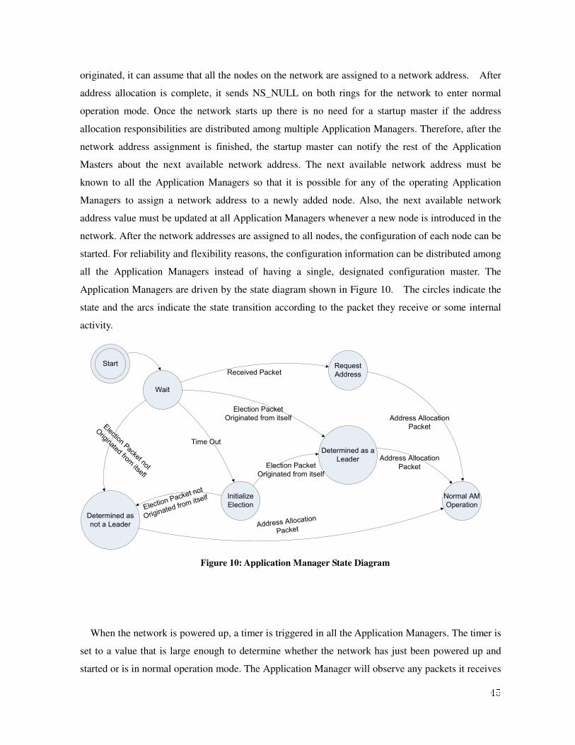
45

originated, it can assume that all the nodes on the network are assigned to a network address. After

address allocation is complete, it sends NS_NULL on both rings for the network to enter normal

operation mode. Once the network starts up there is no need for a startup master if the address

allocation responsibilities are distributed among multiple Application Managers. Therefore, after the

network address assignment is finished, the startup master can notify the rest of the Application

Masters about the next available network address. The next available network address must be

known to all the Application Managers so that it is possible for any of the operating Application

Managers to assign a network address to a newly added node. Also, the next available network

address value must be updated at all Application Managers whenever a new node is introduced in the

network. After the network addresses are assigned to all nodes, the configuration of each node can be

started. For reliability and flexibility reasons, the configuration information can be distributed among

all the Application Managers instead of having a single, designated configuration master. The

Application Managers are driven by the state diagram shown in Figure 10. The circles indicate the

state and the arcs indicate the state transition according to the packet they receive or some internal

activity.

Start

Wait

Request

Address

Initialize

Election

Determined as

not a Leader

Determined as a

Leader

Received Packet

Election Packet

Originated from itself

Election

Packet n

ot

Originate

d from it

self

Election Packet

Originated from itself

Election Packet not

Originated from

itsefl

Normal AM

Operation

Address Allocation

Packet

Address Allocation

Packet

Address Allocation

Packet

Time Out

Figure 10: Application Manager State Diagram

When the network is powered up, a timer is triggered in all the Application Managers. The timer is

set to a value that is large enough to determine whether the network has just been powered up and

started or is in normal operation mode. The Application Manager will observe any packets it receives

46

on the primary ring before the timer reaches zero in order to determine if it has been newly added to

a network that is already running. If it receives any packets, it knows that the network is already

running, so it then will notify an active Application Manager to obtain a network address. If the

Application Manager does not receive any packets before the timer reaches zero, the network has not

yet started. If this is the case, the startup master election process takes place. The election is based on

a unique hardware property called a Slot ID which is a numeric value derived from a PEBB’s

physical location [21]. The Application Manager with the highest Slot ID is elected as the designated

startup master. The LCR algorithm is used for the election process and is done in the following

manner [21].

var statep

begin

statep=“unknown”;

value:=SlotID;

send value to Nextp;

while statep ≠ “leader” do

begin

receive a message v;

if v = value

then statep:=“leader”

else if v > value

then value := v;

end

end

Application Managers broadcast their Slot ID. Each Application Manager consumes the broadcast

message if it discovers a message that originated from an Application Manager with a lower Slot ID.

When an Application Manager Controller receives a message with its own Slot ID, this indicates that

it has been elected as the designated startup master. After a designated startup master is elected, the

network address assignment process is the same as that proposed for PESNet 2.2. As the network

address assignment is finished when the network address allocation packet is received by the

designated startup master, the network is prepared for the nodes to communicate normally using

assigned network addresses.

5.2.2 Hardware Manager Implementation

Unlike the Application Managers, the Hardware Managers are not involved in the startup master

election process. Therefore, they can remain idle until the election process ends. Recall that the

47

network enters normal operation mode when the startup master is elected among the Application

Managers and initiates an address allocation packet on the primary ring and begins to send

NS_NULLs on the secondary ring. When a Hardware Manager is added to a network that is already

running or when it has recovered from a failure, it will observe packets containing regular network

traffic. Therefore, the Hardware Manager knows that the network is already in normal operation

mode and will not receive an address allocation packet unless it notifies one of the active Application

Managers. The Hardware Manager must give one of the active Application Managers an indication of

its existence. Notification of its existence is done by sending an address request to the Application

Manager group address. As explained earlier, the nearest Application Manager can then issue an

address allocation packet on the network for the newly added node.

During normal network startup, the Hardware Manager can remain idle when packets for the

election process among the Application Managers are observed, since it is guaranteed to receive an

address allocation packet as soon as the election process is completed. The behavior of the Hardware

Manager is shown in the state diagram in Figure 11. Once again, the circles are the sate of the

Hardware Manager, and the arc is the transition among the states depending on the received packets.

Figure 11: Hardware Manager State Diagram

48

Chapter 6: Changes to PESNet and Implementation

As features to increase the reliability of the PESNet are added, changes to the packet structure of

PESNet are needed. The changes that should be made to the packet structure are discussed in this

chapter. The changes to the packet structure involve adding additional fields for the information

needed to provide the features that has been discussed in the previous chapters. Before the changes

that should be made are discussed, the packet structure of the current version of PESNet (PESNet

2.2) is briefly introduced. Then the required information for supporting the new features discussed in

the previous three chapters will be examined. As the required information is determined to support

the new features, attempt to add new fields to the packet structure is made.

6.1 Packet Structure of PESNet 2.2

The packet structure of the current version of PESNet contains 8 fields. To provide flexibility,

PESNet can operate in either full mode or reduced mode. When the power electronics application

requires a high switching frequency, PESNet can operate in reduced mode to reduce packet

transmission time between nodes. The tradeoff between operating in reduced or full mode is the

amount of data that can be exchanged by a single packet is reduced in order to similarly reduce the

length of a network tick. Also, the maximum number of nodes in the network is significantly smaller

for reduced mode, since the address field has 2 bits less than that of when operating in full mode.

Table 1 specifies the basic packet structure that is used in PESNet 2.2 and describes each field.

Different types of packets are determined by the CMD field, and each package type contains different

data types, so the format of the data contained in the payload varies for different packets.

49

SYNC CMD DST

ADDR

SRC

ADDR

NET

TIME

FAULT

ADDR

DATA

ARRAY CRC

Full

Mode 8 bits 4 bits 8 bits 8 bits 8 bits 8 bits 80 bits 8 bits

Reduced

Mode 8 bits 4 bits 6 bits 6 bits 6 bits 6 bits 32 bits 8 bits

Basic PESNet Packet Structure

Field Description

SYNC For byte alignment

CMD The command which describes the type of the packet

DEST ADDR The address of the node which the packet is destined to

SRC ADDR The address of the node which sent the packet

NET TIME The current value of the global network clock

FAULT ADDR The address of a fault node

DATA ARRAY The payload of the packet

CRC Cyclic redundancy check

Field Description

Table 1: PESNet 2.2 Packet Structure and Description

6.2 Required Changes to the Packet Structure

Changes to the packet structure must be made and new packet types must be defined in order to

support the new features discussed in the previous chapters. We examine the required information

that is not present in the current packet structure and the additional types of packets that are needed

to support the new features.

6.2.1 Changes Related to Utilization of the Secondary Ring Utilization of the secondary ring involves fault detection and determining the type of fault that has

occurred. During the determination process, the node that detects the failure must have knowledge of

the previous node’s network address—the address of its upstream neighbor. Since the configuration

50

of the network is expected to dynamically change during operation, the network address of the

previous node on the primary ring may change over time as faults, recoveries, and node insertions

occur. The dynamic nature of the network makes it difficult to keep track of the network address of

the previous node. It is difficult to guarantee that the next node is aware of a node’s address and

difficult to determine when to perform updates. Also, the determination of the type of fault may turn

out to be wrong if updating the next node’s previous node’s address is based on packet transmission.

The determination may turn out to be incorrect because newly added nodes do not have a network

address for a certain amount of time when added to the network and there are cases when packets are

queued in a node and may not be able to be sent immediately. For these reasons, it is safer to imbed

the previous node’s address information into every packet.

When a fault is detected from the primary ring in the previous PESNet 2.2 version, the address of

the previous neighbor on the primary ring is sent along the packets that passes the node. However,

there is no way to determine if the fault resulted from a node failure or a link failure. The field name

FAULT ADDR in the packet header is misleading. Moreover, the nodes that receive a packet that

contains a valid address value in the FAULT ADDR field should be able to determine whether the

node with the address contained in the FAULT ADDR field has failed. A more precise indication of

the fault situation in the network may allow the running application to react to the fault more

appropriately. Also, it would be helpful for debugging purposes.

When a node or a link recovers from its failure, there must be a scheme to reestablish

communication with the node that was disconnected and let the network exit failure mode and begin

healing. As described in Chapter 3, this process requires a handshake between the previously

disconnected nodes. Currently, there are no packet types to perform this process.

Also, there is a need to determine when packets in the secondary ring must be forwarded to the

primary ring. The task of forwarding the packets in the secondary ring to the primary ring during the

healing process is primarily done by the healing node. However, recall that there are cases when an

attempt to forward a packet to the primary ring fails at the healing node and the packet is forwarded

onto the secondary ring instead. When a packet on the secondary ring has passed the healing node, it

must be forwarded to the primary ring whenever possible. Therefore, there must be an indication of

whether the packet on the secondary ring has passed the healing node.

51

6.2.2 Changes Related to Silent Failover

Based on the decision to use active replication to support transparent failover, communication

between nodes that involve requesting information and responding to the request will use

multicasting of the request and piggybacking of the response on the rebroadcasted request. In order

to piggyback the response to a request, there must be an additional field that can convey the response.

Also, because only one Hardware Manager responds to a request by an Application Mananger, its

replicas must be able to distinguish whether the request has been processed and serviced at another

node.

6.2.3 Changes Related to Dynamic Reconfiguration

Dynamic reconfiguration of the network involves configuring nodes without a network address.

All nodes do not have a network address when the network has just started up. When the network has

initially started, packets that do not contain any value in the SRC ADDR and DEST ADDR field

must be exchanged. A new type of packet that can perform the startup master election process must

be present. Also, after the new startup master is elected, the network address allocation process starts.

A packet that performs the network address allocation process is needed. After network addresses are

assigned to all the nodes, group address must be allocated to the sets of nodes that replicate each

other. Therefore, packets that can be used for electing the startup master, allocating addresses, and

assigning group addresses are needed.

6.3 Overall Changes to PESNet Packet Structure

In order to support the new features described in this thesis, PREV NODE, FAULT CHECK,

MOVE UP, and RESP were added as new fields in the basic packet structure. PREV NODE is a new

field that contains the address of the previous node upstream. Therefore, a node will replace the field

with its own address before forwarding a packet. FAULT CHECK is a new field that indicates

whether the node address in the FAULT ADDR field has been confirmed to be faulty. MOVE UP is a

new field that indicates whether the packet should be forced upward from the secondary ring back

onto the primary ring because it has already passed the healing node during the healing process.

52

RESP is a new field that contains piggybacked response data when one Hardware Manager in a

group of replicas has already processed the corresponding request held in the remainder of the packet.

The RESP field will not be used when the packet does not request any information from the

destination node. The new packet structure is shown in Table 2.

SYNC CMD DST

ADDR

SRC

ADDR

PREV

ADDR

NET

TIME

FAULT

ADDR

FAULT

CHECK

MOVE

UP

DATA

ARRAY RESP CRC

Full

Mode 8 bits 4 bits 8 bits 8 bits 8 bits 8 bits 8 bits 1 bit 1 bit 80 bits 72 bits 8 bits

Reduced

Mode 8 bits 4 bits 6 bits 6 bits 6 bits 6 bits 6 bits 1 bit 1 bit 32 bits 24 bits 8 bits

Table 2: New Packet Structure for PESNet

The default value of the FAULT ADDR field will be replaced with the PREV ADDR that was

provided by the previous packet when a node detects a failure on the primary ring. When the packet

with the address of the node that could have possibly failed in the FAULT ADDR arrives at the other

end of the point of failure, it is possible to determine whether or not it is a node failure. If it is a node

failure, the FAULT CHECK field can be replaced with value one instead of the default value zero.

On the other hand, if the failure is a link failure, the FAULT CHECK field remains zero. The MOVE

UP field is toggled from the default value of zero to one when the packet passes the healing node on

the secondary ring during the healing process. The FAULT ADDR and FAULT CHECK fields are

cleared in packets that are forwarded from the secondary ring back up to the primary ring. After

healing has been complete, for packets on the primary ring where the FAULT ADDR and FAULT

CHECK fields are non-zero to indicate a fault situation, the two fields are cleared at the healing node.

Originally, a response to a request is performed in PESNet 2.2 by replacing the data in the request

packet with the response data and forwarding the package back to the Application Manager. However,

since the request also must be received by all other replicas, the data comprising the actual request

must stay in the forwarded packet, and the response then must be piggybacked to the request.

Therefore, the packet size had to be increased. The size of the additional field was determined by

analyzing the packets that request data from other nodes. There are four types of packets that are

request packets. They are NS_NORMAL, NS_GET_SYNC, NS_GET_ASYNC, and

NS_REQ_PARAM. Among these packets, NS_NORMAL requires the largest amount of space for

piggybacking. Therefore, the required minimum additional space is bounded by the NS_NORMAL

packet. The size of the response for an NS_NORMAL packet is eight bytes for full mode and two

bytes for reduced mode. However, nine bytes and three bytes are allocated in the RESP field for full

mode and reduced mode, respectively. As the fields of the packet must be allocated in multiples of

53

the size of the information it contains, the additional byte enables request packets other than

NS_NORMAL to contain additional information while 1 byte must be wasted when the additional

byte is not present.

The new packet types that are used for supporting the new features in PESNet can be added to

PESNet by creating new commands. Four bits are allocated to the CMD field, which contains the

command and indicates the type of packets. Thus, sixteen different commands are available in

PESNet. PESNet 2.2 defines ten commands, leaving room for six more. Six is more than enough to

create the new types needed to support the new features. Also, the commands can be subdivided into

more types using the payload of the packet. In other words, the CMD field and the DATA ARRAY

field can be used in combination for new commands. Therefore, there is plenty of room left for

creating new commands. Moreover, sub-typing the commands may be good practice to isolate the

responsibilities of different types of packets.

54

Chapter 7: Analysis of the Protocol In this chapter we analyze the performance of PESNet after the proposed changes. Although some

analysis of the protocol has already been done in Chapter 4, we analyze the protocol’s characteristics

such as the maximum switching frequency and the reliability of the protocol in more detail. Also, a

more accurate analysis of the affect of piggybacking the response in the multicast request packet is

presented. The analysis results support the decisions made throughout the research for PESNet.

7.1 Maximum Switching Frequency

One of the important properties of PESNet is the maximum switching frequency that the

Application Manager is allowed to operate on. The switching frequency of a power electronics

application is the number of adjustments that can be made to the power converter in one second. The

switching frequency heavily depends on the time it takes for a request to receive a response, which

we call a communication cycle. By the nature of the ring topology the network delay for a

communication cycle is the time it takes for a packet to propagate through the entire ring. A

communication cycle cycleT can be easily calculated as the following.

hTT

TTT

TTT

tickcycle

processdelaytick

npropagatiotransmitdelay

×=

+=

+=

)(

Where,

transmitT is the time required for transmitting a packet

npropagatioT is the time for a packet to propagate through the link to the next node

tickT is equivalent to a network tick

processT is the time a packet spends inside a node being routed from one incoming receiver to the

next outgoing transmitter

55

h is the number of network hops required to traverse the entire ring

transmitT can be calculated as

(bits/sec)link theofbandwidth

10(bits)/8packet of size ×. The reason we use

10(bits)/8packet of size × instead of the packet size itself is because 4B/5B encoding is used

when data is transmitted in the transmitter. Data is transmitted in bytes, and each byte is encoded into

a 10 bit data. npropagatioT can be calculated as m/sec)103(light of speed

(m)link theoflength 8×

.

Once we calculate the cycle time, we can obtain the maximum switching frequency which the

protocol allows by calculating cycleT

1.

Let us assume that a network consists of n nodes, all the links are 1 m long, bandwidth is

125Mbit/sec, and packet size is 208 bits as described in Chapter 6 when piggybacking the response to

the multicast request. Then,

processtick

npropagatio

transmit

TT

m

mT

bits

bitsT

+=

≈×

=

=×

=

sec1633.2

nanosec3.3sec/103

1

sec1600.2sec/10125

270

8

6

µ

µ

Usually, it takes n network ticks for a packet to propagate the entire ring and complete one

request and response cycle when no faults are introduced in the network. Therefore, the minimum

cycleT that the protocol can guarantee is nTtick × during normal operation. When there is a link

failure, 2n network ticks are required for a packet to travel around the ring and complete a request

and response cycle. Therefore, the minimum cycleT that the protocol can guarantee is nTtick 2×

when a link failure occurs. However, the maximum switching frequency must be bound by the worse

case. The worse case occurs when there is a node failure. The network’s diameter not only becomes

larger but the time it takes to confirm the node failure and retransmit the lost packet also requires

more time. The total time for a single request and response to complete is 33 −n . Therefore, the

56

minimum cycleT that the protocol can guarantee is )33( −× nT tick when a node failure

occurs. If the system must operate at a higher frequency and require short cycle time, the system can

operate to tolerate link failure only. However, the system may have to halt when a node failure occurs

in that case. If the system requires even shorter cycle time for higher frequency, the system can

operate without tolerating any failure. The system may have to halt when any kind of failure occurs

during operation of the application in that case.

Once we calculate the cycle time, we can obtain the maximum switching frequency which the

protocol allows by calculating cycleT

1. Thus, maximum frequency the protocol can achieve

is)33(

1

−× nTtick

. The following graph shows the maximum switching frequency allowed for

different number of nodes and the faults that can be tolerated. The value of processT is sec1200.0 µ

as it is the minimal time which guarantees the completion of processing a packet [22].

Full Mode

050100150200250300

3 4 5 6 7 8 9 10 11 12 13 14 15Number of NodesSwitching Frequency (KHz) . (Full)Link & Node(Full)Link(Full)Normal(Reduced)Link & Node(Reduced)Link(Reduced)Normal

Figure 12: Switching Cycle for Different Number of Nodes and Operating Mode

The maximum switching frequency value is obtained analytically and the actual value must be

slightly lower if all requests are issued simultaneously at the Application Manager, because the

transmission of a request may be delayed due to queuing. Also, the maximum performance of the

protocol may be reduced if other packets rather than data request packets are issued frequently.

57

7.2 System Reliability with PESNet

The proposed changes to be made to PESNet involve increasing the reliability of the protocol itself.

The point of increasing the reliability of PESNet was to increase the system’s overall reliability and

tolerance of faults. Thus, measuring the reliability that a system can gain by using PESNet is

worthwhile. Evaluating the gained reliability when using PESNet after the changes proposed here is

also meaningful because the overall reliability of the system is affected by any links and nodes added

for redundancy, which increases the possible points of failure. The evaluation shows whether the

reliability has increased. A system that uses PESNet is operational as long as the following

requirements are satisfied:

1. All the required Hardware Managers are present and visible to the network.

2. There is no more than one link (or link pair) failure in the ring.

3. There is no more than one node that has failed at any given time.

Note that if more than one node fails, or if links connecting more than two nodes fail, the dual ring

will be partitioned into two or more completely disconnected regions, with no communication

possible between nodes in separate regions, preventing correct operation of the system. If any of

these three conditions are not met, the system will fail and PESNet will not guarantee normal

operation. Even though the network can be operable with multiple link and node failures, the system

is not able to tolerate multiple failures because it may cause the network to partition and more than

one packet can get lost. The probability of a link or node physically failing can vary depending on the

system’s environment, the hardware it uses, and other factors. Assuming that the reliability of each

network component is provided, we can get a sense of how much the reliability of the system can be

increased after the proposed changes have been made to PESNet.

Let s be the required number of different sets of Hardware Managers and hj denote a Hardware

Manager. Also, let j indicate the type of Hardware Manager which belongs to set j where j<s. Since

the protocol can only permit one node to fail, each set of Hardware Manager has two replicas. In

other words there are two Hardware Managers for each set. Let )(tRc denote the reliability of

component c which is the probability of component c not to fail before time t. Provided that we know

58

the reliability of each type of node that belong to a set, reliability of a node hj can be represented

as )(tRjh . Similarly, the reliability of the Application Manager and the link can be represented

as )(tRAM and )(tRlink . If we assume that all the links are equally reliable, the reliability of the system

can be calculated as the following.

First, we calculate the probability where no nodes has failed and where one node fails for each set

of Hardware Managers.

For an arbitrary Hardware Manager set a

Probability of no failed node in set a is

( )2)()(2 tRtR

aahh

=

Probability of one node to fail in set a

)())(1(2)(1 tRtRtRaaa

hhh×−×=

Then we calculate the probability of no link failing and the probability of one link failing.

Probability of no link failure

(there are 2(2s+1) links since there are 2s+1 nodes and 2 links are used to interconnect each node)

∏+

=

=)12(2

1

)()(s

i

linklinktRtR all

Probability of one link failure

−××+= ∏

−+

=

))(1()()12(2)(1)12(2

1

tRtRstR link

s

i

linklinkone

59

Then the reliability of the system )(tS can be calculated approximately by adding the probability of

the following three cases.

)()()()( 321 tRtRtRtS ++= where

1. There is no link or node failure

)()()()(1

0

1 2 tRtRtRtR allj link

s

jhAM ××= ∏

−

=

2. There is no node failure, but one link failure

)()()()(1

0

2 2 tRtRtRtR onej link

s

jhAM ××= ∏

−

=

3. There is no link failure, but one node failure

( )∑ ∏−

=

−

=

××

−××=

1

0

1

0

2

3 )(2)(

))(1()()()(

s

j

s

ilink

h

h

hAM tRtR

tRtRtRtR all

j

j

i

In order to analyze the gained reliability by allowing failover, we calculate the reliability of a

system using the original version of PESNet. Even though the original version of PESNet did not

implement the use of secondary ring, the analysis assumes that the secondary ring is utilized for link

failure. On the other hand, a node failure may not be tolerated.

The reliability of the system using the changed protocol is affected by two factors. The increased

number of links and the additional nodes which brings redundancy affects the reliability of the

system in two different ways. Depending on the reliability of the added components, the reliability of

the system can decrease. The additional links and node makes the network less reliable, but the

additional nodes make the system more reliable provided that the network has not failed. Therefore it

is assumed that the reliability of the nodes and links each have the same reliability. This assumption

makes it possible to see the how the reliability of the system is affected by the increased number of

nodes and links mutually. To be consistent with the calculation done previously, the variable names

are used as the same. However, since we assume that all nodes have the same reliability )(tRn can be

used for both )(tRAM and )(tRjh .

The reliability of a system that uses the original PESNet can be calculated similarly to the

60

calculation done for the changed PESNet. Since the number of nodes has decreased due to not

allowing duplicate Hardware Managers, the number of links has decreased. Therefore, the probability

of no link failure and one link failure in the network must be recalculated.

Probability of no link failure

( ) )1(2)1(2

1

)()(+

+

=

=∏s

link

s

i

link tRtR

Probability of one link failure

( )

( ) ( ) ( )( )( ))(1)(12

)(1)()1(2

1)1(2

1)1(2

1

tRtRs

tRtRs

link

s

link

link

s

i

link

−××+=

−××+

−+

−+

=

∏

Consequently, the reliability of the system can be approximately calculated by the sum of the

probability of the following two cases.

)()()( 21 tRtRtS′

+′

=′ where

1. There is no link or node failure

∏∏+

=

−

=

××=′

)1(2

1

1

0

1 )()()()(s

i

link

s

j

hAM tRtRtRtRj

2. There is no node failure, but one link failure

−××+××=

′∏∏

−+

=

−

=

))(1()()1(2)()()(1)1(2

1

1

0

2 tRtRstRtRtR link

s

i

link

s

j

hAM j

An attempt to present the gained reliability mathematically by subtracting the two formulas was

made. The new formula indicates the difference in the probability of the system to operate without

failures for time t after it has started. However, the result is too complicated to simplify and

observing the gained reliability from the formula is difficult. To get a better feeling for the reliability

that we gain from the changed protocol, actual numbers were plugged into the formula to acquire the

gained reliability. Values ranging from 0.9 to 1.0 were used for the reliability of the nodes and 0.95 to

1.0 were used for the reliability of the links. This was done for four settings where the required

number of Hardware Manager types were 2, 3, 4, and 5. The results are shown in Figure 13.

61

As Figure 13 shows, the reliability of the links has a greater effect on overall system and network

reliability than that of the nodes. The decrease in reliability when the reliability of the link drops is

significant and has more effect when the number of links increases as the number of nodes increases.

Also, the graphs indicate that the increase in reliability by allowing failover is only guaranteed when

the links are relatively more reliable than the nodes. When the reliability of the nodes is very high,

the increase in the reliability of the system is almost negligible.

Figure 13: Gained Reliability

Table 3 shows the reliability of the system depending on the link and node reliability before and

after the fault tolerant feature is added. The figure shows whether or not the reliability gain we earn is

significant in a practical point of view.

62

PESNet Reliability Before Adding

Fault Tolerance

PESNet Reliability After Adding Fault

Tolerance

2 Sets of

Hardware

Manager

3 Sets of

Hardware

Manager

4 Sets of

Hardware

Manager

5 Sets of

Hardware

Manager

Table 3: Actual Reliability of System Using PESNet

63

The results show that the reliability that we gain by making PESNet fault tolerant is not so

significant unless reliability of the links is close to 1. If the reliability of the link is not close to 1, but

rather low, the reliability gain is not neglectable. If the reliability gain is not so significant, the gain

we earned through the change to the protocol may not be so practical..

64

Chapter 8: Conclusion

The PESNet protocol was developed to support the real-time characteristics of PEBB-based power

electronics applications. It is in a premature state and this thesis describes efforts to improve the

protocol. In spite of the suggested modifications in the thesis, the protocol still poses additional

issues. This chapter is a summary of the changes proposed for PESNet and how the research was

done. This chapter also describes the problems remaining in PESNet, providing directions for future

development of the protocol.

8.1 Summary

The research in this thesis aims to increase the reliability and flexibility of the protocol. The

research focused on allowing PESNet to perform failover among duplicate Hardware Managers. In

order to allow failover among duplicate Hardware Managers, additional features were needed. The

required features that relate to enabling failover each are independent in the sense that they not only

support the failover process, but also can be used alone or to support other features. Certain changes

were made solely for the failover process, but utilization of the secondary ring and dynamic

reconfiguration were also required for the failover process. Therefore, the thesis discusses how

failover can be performed among duplicate Hardware Managers along with utilizing the secondary

ring and dynamic reconfiguration of the network.

8.1.2 Utilizing the Secondary Ring Although the idea of utilizing the secondary ring has been around and planned for PESNet, only

the hardware was designed to provide this feature. No software or firmware for managing this feature

in protocol was implemented prior to this work. The idea of using the secondary ring has been

published in conference papers but it only specifies the basic behavior without much implementation

detail. Therefore, the essential parts of utilizing the secondary ring such as detecting failure,

65

triggering ring-wrap operations, and the healing process were formalized. Failure detection involves

how the network can distinguish a link failure and a node failure. Also, preventing lost packets when

a node failure occurs has been discussed. Finally, the primary ring recovery process is discusses how

the recovered node initiate communication with neighboring nodes again and how to forward the

packets remaining in the secondary ring to the primary ring.

When a failure occurs it is detected by the receiver of the node and enters failure mode. When

either of the links between two nodes fails, both links are considered to be broken. This is to trigger

ring-wrap operation on both ends of the point of failure. A proper forwarding mechanism for the

packets is provided in Chapter 3, and buffers are present to preserve lost packet information due to a

node failure. When a failure is detected, packets are now forwarded through the alternative path

which the secondary ring created and the protocol determines whether it was a link failure or a node

failure. A packet which was sent prior to the failure is kept in a buffer for retransmission when it is

determined that the failure was caused by a node failure. The ring has to recover from the failure

mode once the failed node recovers from the failure. The neighboring nodes of the failed node start

to establish connection as soon as the ring-wrap operation finishes. By continuously making attempts

to establish normal connection, it requires a three-way handshake between the failed node and each

of the neighboring nodes. Once the failed node has confirmed that both sides of the point of failure

has recovered, the network exits the ring-wrapped state and enters healing mode. Healing is done by

forwarding remaining packets in the secondary ring to the primary ring. The node that is responsible

for forwarding packets to the primary ring during healing mode is the called the healing node.

8.1.3 Silent Failover By providing specific details of how the secondary ring can be utilized, another level of reliability

was expected to be reached by allowing redundant Hardware Managers. Failover among redundant

Hardware Managers was a feature that is newly proposed. There were two important issues when

searching for a scheme to make failover possible. One issue was to maintain consistent state among

the replicated Hardware Managers and the other issue was the speed of the failover process. Two

methods to provide failover in the protocol were discussed. By studying the tradeoffs of both Passive

and active replication, we chose to use the active replication approach. Adopting the active

replication scheme in PESNet for silent failover introduced more problems. In the active replication

approach, a node that makes a request multicasts the request to a set of nodes. Therefore, an attribute

66

named group address is required for each node. The group address is introduced to target packets to

be targeted to a certain group of nodes. Multicasting through group address allows the set of nodes

receiving the request to maintain consistent state.

However, the network may become saturated if multiple nodes respond to a single request because

each recipient must send a response packet and also forward the multicast packet at the same time.

Many ideas to reduce this problem were discussed and the final decision was to piggyback the

response in the multicast packet. The main drawback to this method is that the packet size becomes

larger. However, the piggybacking method was chosen because it has more advantages. First of all,

we get better performance when synchronizing actions of Hardware Managers. Also, by having only

one Hardware Manager to reply to a multicast request packet reduces the newly generated packet on

the network. Moreover, depending on the application that is running on PESNet, the packet size can

be reduced by decreasing the size of the field where the response is placed in the packet. This is

possible because the format of the payload part of the packet is predetermined by the application and

all the nodes are aware of the format.

8.1.4 Dynamic Reconfiguration Although the network can tolerate node failure, there is problem when a failed node recovers. If

the recovered node has lost its network address, the node cannot be used until a network address is

reassigned. The original version of PESNet does not have the ability to reconfigure the network as

nodes drop out of or re-enter the network. Therefore, a dynamic configuration scheme was needed to

allow nodes to re-enter the network after recovering from a failure. Dynamic reconfiguration allows

the node to examine the network first to see whether it has been added to a network which was

already operating. The node makes this determination by observing the network traffic. If the

network is in operation, the new node sends out a packet that indicates its presence in the network.

When an Application Manager picks up the packet, it can broadcast an address allocation packet in

response. After a network address is assigned to the new node, it can request a group address for

multicasting. Then the node requests configuration parameters from the Application Manager. As

soon as the node is configured, it can operate normally. On the other hand, if the network is

determined to be in the startup stage, the behavior of the node differs depending on its role in the

network. If the node is an Application Manager, it will begin the startup master election process.

Once the startup master is selected, the startup master assigns network addresses and group addresses

67

to all other nodes in the network. Removing a node and inserting it again in the network is handled

the same way as a node recovering after completely failing. Therefore, hot-swap becomes possible.

8.1.5 Overall Summary

This thesis provides implementation directions for PESNet 2.2 to achieve fault tolerance. A fault

tolerant network is possible by making the secondary ring usable, allowing duplicate Hardware

Managers for silent failover, and supporting dynamic reconfiguration of the network. The three

requirements of the protocol allow it to take advantage of the counter-rotating dual-ring topology. By

making the network fault tolerant instead of using the original PESNet, and by adding dynamic

network reconfiguration feature, hot-swap and plug-and-play also become possible.

8.2 Remaining Problems and Future Work

Although the research was focused on increasing reliability, the analysis in Chapter 7 shows that

the improvement is modest. The maximum reliability gain is slightly more than 0.1 increase in

probability not to fail for time t. Nonetheless, depending on the reliability of the links and nodes, the

reliability gain is negative. Also, the reliability that we gain becomes very small as the reliability of

the nodes increases. The improvement is small because of the fact that the components of the

network such as nodes and links are arranged in series rather than in parallel. The network can

tolerate a link or a node failure and remain to operate normally since the network can remain in a

series configuration due to the secondary ring. However, the network would not be able to allow

more than one link or node to fail as the network can be partitioned and some nodes may not be

visible to the Application Manager. The reliability gain can only be practically significant if the links

are very reliable, which means it is not likely to fail. Otherwise, the benefit we gain by making the

protocol fault tolerant may not be practical because of the cost of the system rises as redundant

components are needed.

The network may not become partitioned as two neighboring Hardware Managers fail. Also, if the

two neighboring Hardware Managers are not replicating each other, the system may be able to

remain normal operation. However, currently this is not possible because packet loss that results from

68

multiple node failures cannot be resolved. To improve the reliability of the system, the protocol must

be able to handle packet losses that occur due to a node failure at any given situation.

Protocol stack of PESNet consists of three layers. Three layers might have been enough for the

previous versions of PESNet. The small number of layers made it possible for the protocol to be

simple. However, as more features are added to PESNet to many features are concentrated at one

level of the layer which makes it complicated to make changes to the protocol. Observations of the

features of the protocol may make it possible to divide the protocol stack into more layers which will

result in a cleaner and neater solution.

Therefore, the following are the future research directions for PESNet to make further

improvements.

1. Develop a more complex topology which allows multiple node failures without affecting the

integrity of the network and introduces parallelism among replicated Hardware Managers

2. Develop a method to resolve packet loss due to multiple node failure

3. Develop a method to resolve packet loss due to node failure during failure mode

4. Develop a method to allow logical faults

5. Develop a more sophisticated protocol stack

8.3 Closing Remarks

The protocol is not stable yet in the sense that it is being changed frequently by many people who

are involved in the research. This instability resulted in improper documentation of the history of the

protocol. It is not clear what the current state of the protocol is. There were limitations in developing

a better protocol as formal information on the hardware’s capabilities and specific behaviors of the

protocol was not available. The research of bringing fault tolerance to Hardware Managers and link

failure to increase reliability of PEBB systems was based on many assumptions. If the characteristics

of the Hardware Managers and detailed requirements of power electronics applications were

available, it may be possible to develop a better protocol. It would have been possible to organize the

necessary information during the research, but the lack of documentation of the previous works on

PESNet led to spending most of the research time in understanding the basic concept. It is very

difficult to relate PESNet to other work as it is a domain specific network protocol. The fact makes

69

the situation worse to get the research started from scratch. Proper documentation for all the PESNet

related work must be done and organized to help new researchers continue to develop PESNet. For

that reason, the thesis tries to point out the essential concepts and the problems.

70

References 1. Ericsen, T. and A. Tucker. Power Electronics Building Blocks and potential power modulator

applications. 1998.

2. Dushan B. Boroyevich, S.H.E., Jinghong Guo. Designing Reusable, Reconfigurable Control

Software for Power Electronics Systems. in CPES Seminar 2002. 2002. Blacksburg, VA.

3. Vlatkovic, V. and D. Borojevic, Digital-signal-processor-based control of three-phase space

vector modulated converters. Industrial Electronics, IEEE Transactions on, 1994. 41(3): p.

326-332.

4. Jinghong, G., I. Celanovic, and D. Borojevic. Distributed software architecture of PEBB-based

plug and play power electronics systems. 2001.

5. Celanovic, I., et al. A new distributed digital controller for the next generation of power

electronics building blocks. 2000.

6. Jinghong Guo, S.E., and Dushan Boroyevich, Improved architecture of PEBB plug and play

power electronics systems: Elementary control object (ECO) and dataflow. CPES 2001 Power

Electronics Seminar and NSF/Industry Annual Review, April 2001.

7. Bassi, E., et al. Communication protocols for electrical drives. 1995.

8. Celanovic, I., et al. A new control architecture for future distributed power electronics systems.

2000.

9. Milosavljevic, I., et al. Analysis of converter operation with phase-leg control in daisy-chained

or ring-type structure. 1999.

10. I. Milosavljevic, D.B., and I. Celanovic. Modularized Communication and Control Structure

for Power Converters. in 8th European Conference on Power Electronics and Applications,

EPE. September 1999.

11. Ross, F.E., An overview of FDDI: the fiber distributed data interface. Selected Areas in

Communications, IEEE Journal on, 1989. 7(7): p. 1043-1051.

12. Cidon, I. and Y. Ofek, MetaRing-a full-duplex ring with fairness and spatial reuse.

Communications, IEEE Transactions on, 1993. 41(1): p. 110-120.

13. Raghavendra, C.S. and M. Gerla, Optimal loop topologies for distributed systems. SIGCOMM

Comput. Commun. Rev., 1981. 11(4): p. 218-223.

14. Hengming, Z. and F. Jahanian. Optimization of a real-time primary-backup replication service.

1998.

15. Budhiraja, N. and K. Marzullo. Tradeoffs in implementing primary-backup protocols. 1995.

71

16. Leslie, L., S. Robert, and P. Marshall, The Byzantine Generals Problem. ACM Trans. Program.

Lang. Syst., 1982. 4(3): p. 382-401.

17. Fred, B.S., Implementing fault-tolerant services using the state machine approach: a tutorial.

ACM Comput. Surv., 1990. 22(4): p. 299-319.

18. Jerry Francis, J.G., and Stephen H. Edwards, Protocol Design of Dual Ring PESNet

(DRPESNet), in CPES 2002 Power Electronics Seminar and NSF/Industry Annual Review.

April 2002.

19. Taolue, C., H. Tingting, and L. Jian. Analysis of a leader election algorithm in /spl mu/CRL.

2005.

20. Milosavljevic, I., Power Electronics System Communications, in Electrical Engineering. 1999,

Virginia Tech: Blacksburg, Virginia.

72

Appendix

A-I PESNet Simulator

A-I-a Simulator Assumptions

A power electronics application can be constructed with the required PEBBs in n! different ways

where n is the number of required PEBBs for the application. The performance of PESNet was

determined to slightly vary depending on the configuration of the nodes in the network as packet

generation patterns become more complex. Therefore, the simulator was built based on several

assumptions to approximately measure the performance. The following are the assumptions and the

rationale for making each assumption. (Also in Section 4.3)

� There is only one Application Manager in the network - Since we are focusing on silent

failover among duplicate Hardware Managers, we limit the number of Application Managers to

one and avoid workload distribution among Application Managers. Workload distribution

among multiple Application Managers which is another desired feature is out of the scope of

this thesis and requires other complex issues as Application Manager failure detection and

recovery.

� All the nodes have the same number of replicas except the Application Manager - Having

the same number of replicas for all nodes may not be desirable as the cost and reliability of

each node may differ. However, having less number of replicas for a node will bring positive

effect on the network performance. In order to observe the performance of the network in

general, we assume that all the node have the same number of replicas.

� Replicas are connected consecutively - The set of Hardware Manager that replicate each other

are connected to the identical physical device. As a result, it was determined that it is natural for

the nodes that replicate each other are physically located close together as possible.

� Simulator simulates the execution of the application without the configuration process -

The configuration process of a node is a process that does not occur frequently. The process is

only carried out as soon as the system starts and when a node is newly added to the network or

73

has recovered from a failure. For most of the operation of the system is for communication

between Application Manager and Hardware Managers. The configuration process in the

middle of system operation is determined to cause minor affect on the network performance.

� The protocol simulation is done above the network layer of the protocol - The simulation

illustrates the movement of the data packets above the network layer of the protocol. Physical

layer of the protocol is not implemented in the simulation. The analysis of the protocol

concentrates on the network delay which is the duration of time for a message to reach its

destination after it is determined to be sent from its source node.

A-I-b Simulator Implementation The simulator was implemented in C#. The selection of the language was made for the

convenience of programming graphical user interface in C#. The following is the class diagram of the

simulator and a brief explanation for each class.

Figure 14: Simulator Class Diagram

The Simulator class is the main class of the program which contains the graphical user interface.

74

The simulator is associated with the Driver class and the NetworkDisplay class. The Driver class is

the main class that performs the simulation. The NetworkDisplay class is responsible for drawing the

network to the panel in the simulator class. The Driver class contains the list of nodes and links in the

network which is simulating. The nodes were implemented using inheritance since AM (Application

Manager) class and HM (Hardware Manager) class share many identical properties. The base class of

AM class and HM class contains the attributes which a node generally has such as address, group

address, and attributes that relate to redirecting packets to the proper ring. The derived AM class and

HM class only contains a method which defines how it processes the received packets. A node is

associated with two Transceiver classes, one for each ring. Each Transceiver class is associated with

two Link classes, each for incoming and outgoing links. A Link class is associated with a Packet class

which denotes the packet that it is transmitting.

The simulator is driven by network ticks. To keep the implementation of the simulator simple, the

simulator is driven by performing the continuous tasks at each node in a distinctive manner. The task

at a node at each network tick was divided into three steps. A network tick is divided into steps of

transmitting a packet, receiving a packet, and processing the received packet. Redirection of the

packets is done accordingly to the condition of the links they are connected to during the three steps.

As the simulator is commanded to advance a network tick, the driver invokes the send method on

each node first. After all the nodes transmit a packet by invoking the send method, the driver invokes

the receive method at all nodes. These two steps illustrate a packet being forwarded to the next node.

As the packets advance to the next node by the two steps, the packet is processed at each node by the

driver. The implementation of the simulator gives an illusion of all nodes performing the three tasks

for each network tick concurrently. In order to simulate link and node failures, the simulator was

designed to introduce link and node failure in the network between network ticks manually. Failed

link and node can also be recovered between network ticks manually. The following figure is a

snapshot of the simulator in simulating the PESNet.

75

Figure 15: Snapshot of the implemented Simulator

The first panel is the control panel of the simulator which is used to create the network to simulate

and controlling it. Each time the Generate Network button is pressed, a new network is created in the

simulator according to the three fields Number of Replicas, Number of Groups, and Packet

Frequency. Number of Replicas is the field which defines the number replicas for each group of

Hardware Managers. Number of Groups is the field which defines the number of required Hardware

Managers needed. Packet Frequency is the field which defines the frequency that the Application

Manager generates requests to each set of Hardware Managers. A faulty link can be introduced in the

simulated network by filling the link name in the Fault Link field and pressing the Make Faulty Link

button. Similarly, a faulty node can be introduced in the simulated network by filling in the address

of the node in the Fault Node field and pressing Make Faulty Node button. Faulty link or node can be

recovered by pressing Recover Faulty Link or Recover Faulty Node. Time advances in the simulator

76

by pressing the Tick button. Time that corresponds to one network tick advances as the Tick button is

pressed. To make the simulator convenient, a feature to advance an arbitrary number of network

ticks. When the textbox left to the Tick button is filled with an integer value, the simulator will

advance network ticks corresponding to the value when the Tick button is clicked.

The second panel provides a graphical representation of the network. Each black rectangle

represents a node. In each node there are two colored rectangles. Each rectangle inside a node

represents a transceiver. The outer ring is the primary ring, and the inner ring is the secondary ring.

Links that relate to the primary ring and the secondary ring are each colored in blue and yellow when

they are not faulty. Faulty links are all colored in red. The packets on the primary ring flows in the

clockwise direction and flows in the opposite direction on the secondary ring. In order to see the

packets movement easily, the packets are displayed in the transceivers and on the links. After each

network tick, the packet information is shown in the transceivers. However, when the Tick button is

pressed, the packets are transmitted to the links and the information of the packet which was

transmitted to each link is displayed for a short period of time to assist understanding the movements

of the packets.

The third panel provides information of the activities of the nodes in the network. As a node in the

simulator generates and transmits a packet, receives a packet, or consumes a packet, the action is

logged. The activity log of the nodes provides information which is used as data for the analysis.

1. Ericsen, T. and A. Tucker. Power Electronics Building Blocks and potential power

modulator applications. 1998.

2. Dushan B. Boroyevich, S.H.E., Jinghong Guo. Designing Reusable,

Reconfigurable Control Software for Power Electronics Systems. in CPES Seminar 2002.

2002. Blacksburg, VA.

3. Vlatkovic, V. and D. Borojevic, Digital-signal-processor-based control of three-

phase space vector modulated converters. Industrial Electronics, IEEE Transactions on, 1994.

41(3): p. 326-332.

4. Jinghong, G., I. Celanovic, and D. Borojevic. Distributed software architecture of

PEBB-based plug and play power electronics systems. 2001.

5. Celanovic, I., et al. A new distributed digital controller for the next generation of

power electronics building blocks. 2000.

6. Wu, J., Implementation of a 100kWSoft-Switched DC Bus Regulator Based on

Power Electronics Building Block Concept, in Electrical and Computer Engineering. 2000,

Virginia Polytechnic Institute and State University: Blacksburg, VA.

7. Jinghong Guo, S.E., and Dushan Boroyevich, Improved architecture of PEBB plug

and play power electronics systems: Elementary control object (ECO) and dataflow. CPES

2001 Power Electronics Seminar and NSF/Industry Annual Review, April 2001.

77

8. Bassi, E., et al. Communication protocols for electrical drives. 1995.

9. Celanovic, I., et al. A new control architecture for future distributed power

electronics systems. 2000.

10. Milosavljevic, I., et al. Analysis of converter operation with phase-leg control in

daisy-chained or ring-type structure. 1999.

11. I. Milosavljevic, D.B., and I. Celanovic. Modularized Communication and Control

Structure for Power Converters. in 8th European Conference on Power Electronics and

Applications, EPE. September 1999.

12. Jerry Francis, J.G., and Stephen H. Edwards, Protocol Design of Dual Ring PESNet

(DRPESNet), in CPES 2002 Power Electronics Seminar and NSF/Industry Annual Review.

April 2002.

13. Francis, G., A Synchronous Distributed Digital Control Architecture for High

Power Converters, in Electrical Engineering. 2004, Virginia Polytechnic Institute and State

University: Blacksburg.

14. Ross, F.E., An overview of FDDI: the fiber distributed data interface. Selected

Areas in Communications, IEEE Journal on, 1989. 7(7): p. 1043-1051.

15. Cidon, I. and Y. Ofek, MetaRing-a full-duplex ring with fairness and spatial reuse.

Communications, IEEE Transactions on, 1993. 41(1): p. 110-120.

16. Raghavendra, C.S. and M. Gerla, Optimal loop topologies for distributed systems.

SIGCOMM Comput. Commun. Rev., 1981. 11(4): p. 218-223.

17. Hengming, Z. and F. Jahanian. Optimization of a real-time primary-backup

replication service. 1998.

18. Budhiraja, N. and K. Marzullo. Tradeoffs in implementing primary-backup

protocols. 1995.

19. Leslie, L., S. Robert, and P. Marshall, The Byzantine Generals Problem. ACM

Trans. Program. Lang. Syst., 1982. 4(3): p. 382-401.

20. Fred, B.S., Implementing fault-tolerant services using the state machine approach:

a tutorial. ACM Comput. Surv., 1990. 22(4): p. 299-319.

21. Taolue, C., H. Tingting, and L. Jian. Analysis of a leader election algorithm in /spl

mu/CRL. 2005.

22. Milosavljevic, I., Power Electronics System Communications, in Electrical

Engineering. 1999, Virginia Tech: Blacksburg, Virginia.