Bridging the Gap Between HPC and Big Data Frameworks

Michael Anderson1, Shaden Smith2, Narayanan Sundaram1, Mihai Capota1, Zheguang Zhao3, Subramanya Dulloor4,

Nadathur Satish1, and Theodore L. Willke1

1Parallel Computing Lab, 4Infrastructure Research Lab, Intel Corporation; 2University of Minnesota; 3Brown University

michael.j.anderson@intel.com, shaden@cs.umn.edu, narayanan.sundaram@intel.com, mihai.capota@intel.com,

sam@cs.brown.edu, subramanya.r.dulloor@intel.com, nadathur.rajagopalan.satish@intel.com, ted.willke@intel.com

ABSTRACT

Apache Spark is a popular framework for data analytics withattractive features such as fault tolerance and interoperabil-ity with the Hadoop ecosystem. Unfortunately, many an-alytics operations in Spark are an order of magnitude ormore slower compared to native implementations writtenwith high performance computing tools such as MPI. Thereis a need to bridge the performance gap while retaining thebenefits of the Spark ecosystem such as availability, pro-ductivity, and fault tolerance. In this paper, we propose asystem for integrating MPI with Spark and analyze the costsand benefits of doing so for four distributed graph and ma-chine learning applications. We show that offloading compu-tation to an MPI environment from within Spark provides3.1−17.7× speedups on the four sparse applications, includ-ing all of the overheads. This opens up an avenue to reuseexisting MPI libraries in Spark with little effort.

1. INTRODUCTIONAs dataset sizes increase, there is a need for distributed

tools that allow for exploration and analysis of data thatdoes not fit on a single machine. Apache Hadoop provides afault-tolerant distributed filesystem as well as a map-reduceprocessing framework that allows for analytics on large data-sets. More recently, Apache Spark introduced the resilientdistributed dataset (RDD) which can be cached in memory,thereby accelerating iterative workloads often found in ma-chine learning [34]. In addition to map-reduce-style compu-tation, Spark includes support for joins, as well as extensivelibrary support for graph computations, machine learning,and SQL queries. These applications generally achieve morethan an order of magnitude better performance in Sparkcompared to Hadoop for workloads that can leverage in-memory data reuse.

Despite large speedups compared to Hadoop, Spark’s per-formance still falls well short of the performance achievable

This work is licensed under the Creative Commons Attribution­NonCommercial­NoDerivatives 4.0 International License. To view a copyof this license, visit http://creativecommons.org/licenses/by­nc­nd/4.0/. Forany use beyond those covered by this license, obtain permission by emailinginfo@vldb.org.Proceedings of the VLDB Endowment, Vol. 10, No. 8Copyright 2017 VLDB Endowment 2150­8097/17/04.

with high performance computing (HPC) frameworks thatuse native code and optimized communication primitives,such as MPI [9]. For example, a recent case study found Cwith MPI is 4.6–10.2× faster than Spark on large matrix fac-torizations on an HPC cluster with 100 compute nodes [11].Another case study on distributed graph analytics foundthat for weakly-connected components, one can outperformSpark’s GraphX library by up to two orders of magnitudeon a cluster with 16 compute nodes, with roughly 2000 linesof C++ using OpenMP for shared-memory parallelism andMPI for distributed communication [28].

The Spark environment provides many attractive featuressuch as fault-tolerance, as RDDs can be regenerated throughlineage when compute nodes are lost, as well as program-mer productivity through the use of Scala and high-levelabstractions. We would ideally like to be able to use librarieswritten for MPI and use data that originates in distributedSpark RDDs, allowing users to temporarily trade the ben-efits of the Spark environment in exchange for high perfor-mance. However, this creates several problems. First, RDDdata lives in JVM processes that are not launched within anMPI environment, and it is not immediately obvious howone would configure an MPI environment on the fly start-ing with these processes. Second, even if we could config-ure such an environment on the fly, communicating betweenSpark executors would potentially violate the assumptionsthat Spark makes about RDDs. An RDD depending on anMPI collective operation, for example, would not have thisdependence encoded in Spark’s own bookkeeping and there-fore may not be recoverable in the event of a failure. Dueto these challenges, tight integration of MPI and Spark isgenerally not practiced today.

In this paper, we propose Spark+MPI, a system for inte-grating MPI-based programs with Spark. Our approach is toserialize data from Spark RDDs and transfer the data fromSpark to inter-process shared memory for MPI processing.Using information from the Spark driver, we execute plainMPI binaries on the Spark workers with input and outputpaths in shared memory. The results of the MPI process-ing are copied back to persistent storage (HDFS), and theninto Spark for further processing. This approach requires nochanges to Spark itself, and it can adapt to changes in thecluster, such as adding or removing compute nodes.

We contrast this with an another approach to integrat-ing native code with Spark, which is to accelerate user-defined functions (UDFs) in Spark by calling native C++code through the Java Native Interface (JNI), while retain-

901

ing the use of Spark for distributed communication andscheduling. This optimization technique is commonly em-ployed. For example, many operations in Spark’s machinelearning and graph analysis libraries offload computation tothe Breeze library, which contains optimized numerical rou-tines implemented in either Java or JNI-wrapped C.

To test our Spark+MPI system, we implement four dis-tributed graph and machine-learning applications: LatentDirichlet Allocation (LDA), PageRank (PR), Single SourceShortest Path (SSSP), and Canonical Polyadic Decomposi-tion (CPD). We find that offloading computation from Sparkto MPI using our system can provide 3.1 − 17.7× speed-ups compared to Spark-based implementations on real-worldlarge-scale datasets on a 12-node cluster. This includes timespent transferring data to and from an MPI environment,and any time required for MPI applications to construct anyspecial data structures.

To summarize, our contributions are the following:

1. We propose Spark+MPI, a system demonstrating tightintegration of Spark and MPI, which enables use ofexisting MPI-based libraries in the Spark environment.

2. Our optimization strategies result in 3.1−17.7× speed-ups on sparse graph and machine learning algorithmscompared to Spark-based implementations.

3. We quantify the overheads of Spark and show the lim-its of alternative optimization strategies for augment-ing Spark with native code.

The rest of the paper is organized as follows. Section 2describes related work. Section 3 describes the design andimplementation details of our Spark+MPI system. Section 4describes the four graph and machine learning applicationsconsidered for optimization. Section 5 shows the applicationimplementations and alternative means of increasing Sparkperformance. Section 6 describes our experimental setup,including the hardware and software configuration, profilingtools, and datasets. Section 7 presents performance andprofiling results and analysis, as well as insights gained fromour experiments. Section 8 offers conclusions from our work.

2. RELATED WORKIt has been widely noted that MPI-based HPC frameworks

outperform Spark or Hadoop-based big data frameworks byan order of magnitude or more for a variety of different appli-cation domains, e.g., support vector machines & k-nearestneighbors [24], k-means [14], graph analytics [25, 28], andlarge-scale matrix factorizations [11]. A recent performanceanalysis of Spark showed that compute load was the primarybottleneck in a number of Spark applications, specificallyserialization and deserialization time [22]. Our performanceresults are consistent with this research.

Other work has tried to bridge the HPC-big data gap byusing MPI-based communication primitives to improve per-formance. For example, Lu et al. [19] show how replacingmap-reduce communicators in Hadoop (Jetty) with an MPIderivative (DataMPI) can lead to better performance; thedrawback of this approach is that it is not a drop-in replace-ment for Hadoop and existing modules need to be re-codedto use DataMPI.

It has been shown that it is possible to extend pure MPI-based applications to be elastic in the number of nodes [23]

Time

HDFS

MPI

Processes

Shared

Memory

Spark

Executor

Input

Partition

Input

Partition

Compute

Output

Partition

HDFSWriter

Output

Partition

Output

Partition

Figure 1: Spark+MPI implementation overview: data istransferred from Spark to shared memory for MPI process-ing, then back to Spark through HDFS.

through periodic data redistribution among required MPIranks. However, this assumes that we are still using MPI asthe programming framework, hence we do not get the otherbenefits of processing in the cloud with Spark or Hadoop,such as high productivity or fault tolerance.

Efforts to add fault tolerance to MPI have been ongoingsince at least 2000, when Fagg and Dongarra proposed FT-MPI [8]. Although the MPI standard has still not integratedany fault tolerance mechanism, proposed solutions continueto be put forth, e.g., Fenix [10]. However, there is a largeproductivity gap between the APIs of Fenix and Spark.

Several machine learning libraries have support for inter-operating with Spark, such as H2O.ai [13] and deeplearn-ing4j [7], and include their own communication primitives.However, these are Java-based approaches and do not pro-vide for direct integration of existing native-code MPI-basedlibraries.

SWAT [12], which stands for SparkWith Accelerated Tasks,creates OpenCL code from JVM code at runtime to improveSpark performance. As opposed to our work, SWAT is lim-ited to single-node optimizations; it does not have access tothe communication improvements available through MPI.

Thrill [4] is a project building a Spark-like data processingsystem in C++ and using MPI for communication. UnlikeThrill, our goal is not to build an entirely new system, butrather to augment the existing successful Spark ecosystemwith available performant MPI-based libraries.

3. SPARK+MPI SYSTEM DESIGN AND

IMPLEMENTATIONSpark+MPI bridges the gap between big data and HPC

frameworks by taking the best of both worlds: Spark faulttolerance and productivity, MPI performance. We achievethis by basing our design on RDDs, using the Spark re-source management infrastructure to launch MPI processes,and providing a high-level API that integrates seamlessly inSpark.

We designed Spark+MPI as an extension to Spark whichenables access to standard MPI implementations, thereforeusers are not required to install a special distribution ofSpark or a custom MPI implementation.

3.1 ImplementationWe implemented Spark+MPI using the Linux shared mem-

ory file system /dev/shm for exchanging data efficiently be-tween Spark and MPI. Figure 1 depicts a high-level overviewof our implementation.

902

We begin with data stored in a distributed RDD withinSpark with the goal of using MPI-based libraries to pro-cess the data. The first step is to make the data accessibleto the MPI processes. We serialize and write the data to amemory region mapped to /dev/shm using a mapPartitions

transformation on the RDD that we would like to copy. ThemapPartitions operation produces a partition ID and a hostname associated with each partition, which are collected bythe Spark driver. This collect operation forces Spark to per-form the action and copy the data. Next, the driver usesthe partition information to launch an MPI execution us-ing the standard mpiexec command. The MPI executionreceives a configurable amount of RAM, which is not avail-able to Spark. The MPI execution performs the application-specific computation by consuming the binary data preparedby Spark; it produce new binary data, which is also storedin /dev/shm. When we are done computing using MPI, wewrite the results to HDFS. Then, the results are read fromHDFS into Spark and stored as a new RDD. Since HDFS ispersistent and fault-tolerant, storing the results of the MPIcomputation in HDFS guarantees that they will be preservedregardless of future failures.

3.2 APIThe API of Spark+MPI is composed of Scala and C++

functions. The following Scala functions allow for a tradi-tional Spark program to call an MPI program:

rddToNative(rdd, serializeFn)->inputHandle Thefirst function in the API, rddToNative, prepares anRDD for MPI processing. rddToNative requires a se-rialization function that produces output in the binaryformat expected by the MPI program.

emptyNative(inputHandle)->outputHandle Createsa placeholder for the output of the MPI binary usinginformation about the compute nodes from the RDDpre-processed by rddToNative.

runMPI(inputHandle, outputHandle, binary, args)Calls the MPI binary specified as a file system path us-ing the input and output data handles and additionalapplication-specific arguments.

nativeToHDFS(outputHandle)->hdfsPath Saves theoutput of the MPI binary to persistent HDFS storage.

nativeToRDD(deserializeFn, hdfsPath)->outputRDDMakes the MPI output available to further Spark pro-cessing by transforming it to an RDD. nativeToRDDrequires a deserialization function which builds JVMobjects from the application-specific binary data.

The last two functions in the API, nativeToHDFS andnativeToRDD, can be omitted when building a pipeline thatrepeatedly calls MPI binaries, thus amortizing the cost ofHDFS I/O. Furthermore, these functions can be used as acheckpoint-restore mechanism to balance the advantages ofavoiding HDFS I/O with the risk of compute node failures.

While Spark+MPI works with standard MPI implemen-tations, applications must use our C++ API to access inputand output data:

partition Structure that stores data along with metadataabout the compute nodes used for processing.

θ wzα

φηK

N

J

∼ �����ℎ � �� ∼ �����ℎ �� ∼ � � ��� ∼ � � �� ��

Figure 2: Latent Dirichlet Allocation - graphical model.Only the words are observed. α and η are hyperparame-ters. θj and φk are probability distributions over topics andwords respectively.

binaryFiles(inputHandle)->partitionsIn PreparesC++ input data structures based on the input handlereceived from the Scala API.

savePartitions(partitionsOut, outputHandle) Pre-pares serialized output in the format required by theScala API based on the partitions outputted fromapplication-specific C++ processing.

4. APPLICATIONSWe use the following graph and machine learning algo-

rithms as driving applications throughout the paper: La-tent Dirichlet Allocation, PageRank, Single Source ShortestPath, and Canonical Polyadic Decomposition.

4.1 Latent Dirichlet Allocation (LDA)Latent Dirichlet Allocation (LDA) tries to group docu-

ments (which are modeled as bags of words) into “topics”(which are defined as a probability distributions over words).Figure 2 shows the graphical model used in LDA. For de-tails on the LDA model, we refer the readers to Blei et al. [5].We use Maximum a Posteriori (MAP) estimation using anExpectation–Maximization (EM) algorithm in order to learnthe topic and word distributions [3]. Assuming we have J

documents and a W word vocabulary, each document j hasa word count vector Nwj for word w. This is modeled as abipartite graph of size (J +W )× (J +W ) with edges (w, j)with weights Nwj . α and η are the priors to the Dirichletdistributions θj and φk for k topics, as shown in Figure 2.The EM algorithm works iteratively. At each iteration,

the following updates are performed.

γwjk =(Nwk + η − 1)(Nkj + α− 1)

Nk +Wη −W(1)

γwjk =γwjk

∑

kγwjk

(2)

Nwk =∑

j

Nwj γwjk (3)

Nkj =∑

w

Nwj γwjk (4)

Nk =∑

w

Nwk =∑

j

Nkj (5)

Once the iterations are complete, the MAP estimates ofθ and φ are obtained as

θkj =Nkj + α− 1

Nj +Kα−Kφwk =

Nwk + η − 1

Nk +Wη −W(6)

903

4.2 PageRank (PR)PageRank (PR) is an algorithm used to rank vertices on

the basis of how probable it is for them to be encounteredon a random walk along the edges of a directed unweightedgraph. It was originally used to rank web pages with thepages themselves modeled as graph vertices and hyperlinksas edges. The algorithm iteratively updates the rank of eachvertex according to the following equation:

PRt+1(v) = r + (1− r)×

∑

u|(u,v)∈E

PRt(u)

degree(u)(7)

where PRt(v) denotes the page rank of vertex v at itera-tion t, E is the set of edges in a directed graph, and r is theprobability of random surfing. The algorithm is run untilthe page ranks converge.

4.3 Single Source Shortest Path (SSSP)Single Source Shortest Path (SSSP) is an algorithm used

to find the shortest path from a given vertex to all the othervertices in a directed, weighted graph. The algorithm isused in many applications such as finding driving directionsin maps or computing the min-delay path in telecommuni-cation networks. The algorithm starts with a given vertex(called source) and iteratively explores all the vertices in thegraph to assign a distance value to each of them, which isthe minimum sum of edge weights needed to reach the vertexfrom the source. At each iteration t, each vertex performsthe following:

Distance(v) = min(Distance(v),

minu|(u,v)∈E{Distance(u) + w(u, v)}) (8)

where w(u, v) represents the weight of the edge (u, v). Ini-tially the Distance for each vertex is set to ∞ except thesource with Distance value set to 0. We use a slight vari-ation on the Bellman-Ford shortest path algorithm wherewe only update the distance of those vertices that are ad-jacent to those that changed their distance in the previousiteration.

4.4 Canonical Polyadic Decomposition (CPD)Tensors are the generalization of matrices to higher di-

mensions (called modes). The CPD is one generalizationof the singular value decomposition to tensors and has usesin many applications such as web search [16], collaborativefiltering [26], and others [27]. The rank-F CPD models a

tensor X ∈ RI1×···×IN with factor matrices A(1) ∈ R

I1×F ,. . . , A(N) ∈ R

IN×F . The CPD, shown in Figure 3, is mostintuitively formulated as the sum of outer products.

The CPD is a non-convex optimization problem and mostcommonly computed using alternating least squares (ALS).ALS cyclically updates one factor matrix at a time whileholding all others constant. The matricized tensor timesKhatri-Rao product (MTTKRP) is the bottleneck of ALSand is a generalization of sparse matrix-vector multiplication(SpMV) [17]. When updating the nth factor matrix, theMTTKRP computes the matrix K ∈ R

In×F and uses theremaining (N−1) factor matrices. Suppose the non-zero v

≈ + · · ·+

Figure 3: Tensor decomposition as a sum of outer products.

has coordinate (i1, . . . , iN ). The MTTKRP updates K via:

Kin ← Kin +v

(

A(1)i1∗ · · · ∗A

(n−1)in−1

∗A(n+1)in+1

∗ · · · ∗A(N)iN

)

,

(9)where Mi denotes the ith row of a matrix M and ∗ de-notes the Hadamard (element-wise) product. Like SpMV,distributed-memory MTTKRP requires up to two commu-nication stages: (i) aggregating partial computations and(ii) exchanging the new elements of the factor matrix [15].

5. APPLICATION IMPLEMENTATIONSIn this section we describe our strategies for implementing

and optimizing the aforementioned applications in Spark.First, we consider Spark-based libraries as a baseline. Sec-ond, we consider offloading key computations into optimizedC++ routines and calling these using JNI, while retainingthe use of Spark for distributed communication and schedul-ing. Third, we offload the entire computations from Sparkinto the MPI environment using our Spark+MPI system,which allows us to leverage existing high-performance MPI-based libraries.

5.1 Spark librariesThree of the four applications we consider are readily

available in existing Spark libraries. We use the built-inPR provided by GraphX [33]. For SSSP, we use the Pregelframework in GraphX. For LDA, we use the MLlib [21] im-plementation which is based on Expectation–Maximization(EM), and also uses GraphX data structures and computa-tional primitives. These implementations store both vertexproperties and edges as distributed RDDs, and use shufflesto communicate this data between machines during each it-eration.

We implemented CPD ourselves, as no Spark implemen-tations exist, to the best of our knowledge. Our version usesSpark’s parallel primitives for the distributed MTTKRP op-eration in Equation 9. The results of the MTTKRP opera-tions are collected by the driver. Operations on the factorsare done on the driver node using dense linear algebra rou-tines provided in the Breeze library.

5.2 Optimized SparkRecently, MLlib added support for optimized linear alge-

bra operations on sparse and dense matrices [6]. One sug-gested usage model for sparse matrix operations in Spark isto do matrix operations in a distributed fashion and vectoroperations on the driver. This means that vectors are firstbroadcast to the executors, operated on, and then collectedback to the driver during each iteration of an algorithm.If the vectors do not fit on the driver, then a different setof matrix-vector routines can be used which distribute thevectors as well as the matrices. We implemented our appli-cations following the same communication and computationmodel as Spark’s sparse matrix-vector (SpMV) multiplica-tions [6]. We refer to our implementations as OptSpark.

904

...Tile 0 Tile 1 Tile N

Executor PartitionsDriver

Vector

Vector Vector Vector

Update

(1) Broadcast Vector

(2) JNI Matrix-Vector Op

Update Update

Vector

(3) Collect Updates

0

1

2

…

N

Matrix Layout

Figure 4: OptSpark: iterative sparse algorithms with JNI,modeled after MLlib’s sparse matrix operations. Matrixdata is stored in 1D partitions on executors where it is pro-cess in a distributed fashion, while vector operations takeplace on the driver.

For our applications and hardware configuration, the vec-tors do fit on the driver and so we implemented the applica-tions based on the MLlib 1D SpMV communication pattern,shown in Figure 4. For example, for PR, the graph datasetbecomes a sparse matrix with a nonzero for every edge.In the case of a Twitter follower-followee graph, the vectorstores a single ranking for each Twitter user. The matrixrows (i.e., the Twitter users) are distributed across execu-tors. At every iteration, the vector is first broadcast from thedriver to the executors. For PR and SSSP, a custom matrix-vector operation is implemented using C++ routines madeavailable through the Java Native Interface (JNI). This cus-tom matrix-vector operation is applied to the input vectorand returned to the driver using collect, where it is usedto update the vector for the next iteration.

We implemented OptSpark PR and SSSP using the afore-mentioned approach, with the following implementation de-tails. In order to maximize the granularity of our callsthrough JNI, we merge all rows within a partition of thesparse matrix into a single Compressed Sparse Row (CSR)representation. Each array that is needed inside the nativefunction is accessed using GetPrimitiveArrayCritical toavoid unnecessary copies between Java and native arrays.We assume that the partition ID does not change duringexecution, so we can collect the matrix row indices on thedriver ahead of time which reduces the total size of the col-lect. The driver also uses OpenMP-parallelized JNI func-tions to update the vectors before and after each iteration.

For LDA and CPD, we provide a best-case per-iterationperformance estimate using the following micro-benchmark.We simulate algorithm iterations with the following steps:(1) broadcast random data with type Array[Double] tothe workers, (2) perform a map over each partition of thedataset, where each task copies a portion of the broadcastvariable into a result array, and (3) collect partitions ofthe result array, packaged as (Int, Array[Double]), to thedriver. The broadcast and collected data is sized accordingto the algorithm being simulated. This micro-benchmarkgives us a lower-bound estimate of runtime per iteration, byassuming that the matrix-vector operation compute time isnegligible. For the LDA micro-benchmark we broadcast adense double-precision matrix of size (J+W )×K and collecta matrix of the same size back to the driver. For the CPDmicro-benchmark, we do one broadcast/collect for each fac-tor. Broadcasting all CPD factors at once caused causedproblems in Spark due to the large total size of the factormatrices.

5.3 Spark+MPIFor the Spark+MPI implementation of the applications,

we use two readily available MPI-based libraries.For PR, SSSP, and LDA, we use GraphMat [32], a frame-

work for graph analytics. It provides high performance byleveraging optimized OpenMP-parallel sparse matrix prim-itives. GraphMat was recently extended to distributed sys-tems through the integration of MPI-based distributed prim-itives [2]. Graph data is distributed across nodes in a 2Dblock cyclic format and vertex properties are distributedacross nodes as well. Messages derived from vertex prop-erties are compressed into sparse vectors and sent to othernodes using MPI. Local sparse matrix-vector multiplicationsare parallelized with OpenMP.

For CPD, we use the Surprisingly ParalleL spArse Ten-sor Toolkit (SPLATT), an MPI+OpenMP library for fac-toring large, sparse tensors [30]. It uses a medium-graineddecomposition which distributes an N -mode tensor over anN -dimensional grid of MPI processes [31]. The medium-grained decomposition requires two communication stages,but limits communication in the ith mode to processes thatshare a coordinate in the ith dimension of the process grid.

6. EXPERIMENTAL SETUPTo test the performance of Spark+MPI, we perform ex-

periments on a cluster with up-to-date hardware and soft-ware using datasets representative for the applications weconsider.1

6.1 ConfigurationEach machine in our cluster has 2 IntelR© XeonR© E5-

2699 v4 processors (22 cores, 44 threads each), 128 GiBDDR4 RAM, an SSD, a 1 Gbit/s Ethernet interface, anda 100 Gbit/s IntelR© Omni-Path interface. We use CentOS7.2 (with Linux 3.10), IntelR© Compiler 16.0.3, IntelR© MKL11.3.3, IntelR© MPI 5.1.3, Oracle Java 1.8.0, HDFS 2.7.2,and Spark 2.0.0.

Our cluster has 13 machines. We run the HDFS and Sparkmaster on one machine, the Spark driver on another ma-chine, and 11 Spark workers on the remaining machines inthe cluster. When we run MPI on the cluster, it uses the 12compute nodes (the driver + 11 workers).

Spark is configured to use the G1GC garbage collectorand the Kryo serializer. We considered (1) allowing Sparkto choose the default number of partitions based on the num-ber of HDFS blocks, (2) setting the number of partitions tothe total number of cores, and (3) setting the number ofpartitions to twice the number of cores. We found that (1)provided the best overall performance for all Spark imple-mentations except for CPD which excelled with (3). We usethis setting for our results. We also use the default parti-tioning strategy for GraphX data structures. When Spark isrunning alone, we give 96 GiB of memory for both the driverand the executors. When we run MPI alongside Spark, wegive the Spark driver and executors 80 GiB of memory. We

1Software and workloads used in performance tests may have been op-

timized for performance only on Intel microprocessors. Performancetests, such as SYSmark and MobileMark, are measured using specificcomputer systems, components, software, operations and functions.Any change to any of those factors may cause the results to vary. Youshould consult other information and performance tests to assist youin fully evaluating your contemplated purchases, including the per-formance of that product when combined with other products. Formore information go to http://www.intel.com/performance

905

set the number of driver and executor cores to 88, which isequal to the number of threads the CPUs can execute con-currently, meaning that one executor runs per worker. Whenwe launch MPI, we set the number of OpenMP threads to44, equal to the number of cores in each machine. We runone MPI process per machine.

We disregard the time to initially load input datasets fromHDFS into Spark. Each benchmark begins timing only afterthe input dataset has been loaded from HDFS, stored in anRDD which is cached using cache, and then counted whichensures that the previous tasks complete before moving onto the rest of the application. Because Spark uses lazy ex-ecution, we need to take actions such as these to ensurethat all computations are actually executed at the expectedtime during each benchmark. PR, SSSP, and LDA all pro-duce their outputs in RDDs. We call cache and count onthese outputs to do this, and we include the runtime for thisoverhead as part of the total algorithm runtime. For CPD,both the Spark implementation and Spark+MPI implemen-tation produce outputs on the driver. The overhead timeto transfer these outputs from RDDs to the driver for theSpark+MPI implementation is included as part of the totalalgorithm runtime. We also call cache and count on theSpark data structures after their construction and includethis as part of Spark data structure construction time.

PR, LDA, and CPD all use double-precision arithmeticfor all implementations. For SSSP, we store the depths asInt for all implementations. GraphX represents vertex IDsas Long, while GraphMat and OptSpark store these as Int.

We run PR for 54 iterations, which is the total numberof iterations required for convergence in GraphMat for ourdataset (for Spark and SparkOpt, we set the number of iter-ations to this number). We solve LDA with 20-dimensionalfactors, α and η equal to the Spark defaults (3.5 and 1.1,respectively), and run for 10 iterations. We run CPD with10-dimensional factors for 22 iterations, which is the totalnumber of iterations needed for convergence in SPLATT.SSSP naturally runs the same number of iterations in eachimplementation. Micro-benchmarks run for 10 iterations to-tal and the runtime of the first iteration is discarded.

For system-level performance analysis, we use the sar toolfrom the Sysstat package executed with the Intel Perfor-mance Analysis Tool2. We collect samples every 1 s forCPU usage and network transfer.

To analyze Spark implementations, we developed an eventlog parser that computes aggregate metrics from the Sparkevent log for the following components: scheduler delay, taskdeserialization and result serialization, data shuffling, andalgorithm computation. To identify bottlenecks, we calcu-late the observed time of each of these components whileaccounting for task-level parallelism. For example, to calcu-late the observed data shuffling time for a stage, the parserreconstructs the task events from the timestamps, and thensubtracts the time for data shuffling in each task to com-pute the stage runtime as if without the data shuffling. Theobserved data shuffling time is the difference between thishypothetical stage runtime and the actual stage runtime.

6.2 DatasetsTable 1 summarizes the datasets used in our performance

evaluation. Twitter is a graph of the “follower-followee” re-lationships from 41.7 million user profiles in 2010. We use

2https://github.com/intel-hadoop/PAT

Table 1: Dataset Summary

Dataset Records Record Type

Wikipedia [1] 0.7 billion (DocID, WordID, Count)Twitter [18] 1.5 billion (SrcID, DstID, Weight)Amazon [29, 20] 1.7 billion (UserID, ItemID, WordID, Count)

Twitter for both PR and SSSP. For LDA, we use Wikipedia,a sparse term-frequency matrix formed from 3.3 millionWiki-pedia articles. For CPD, we use Amazon, which is a sparsetensor of user-product-word triplets taken from product re-views. Each non-zero Xuiw in Amazon is the frequency ofword w appearing in user u’s review of product i.

7. RESULTSIn this section, we provide performance evaluation results,

as well as insight into the bottlenecks that are behind theresults.

7.1 Overall performanceTable 2 shows the runtime for all implementations on each

of the four algorithms. These runtimes are broken downfurther into categories:

• Build Time: Time to construct a data structuresneeded for computing the algorithm result, for examplegoing from a collection of records to a graph or sparsematrix data structure. This step can potentially beamortized by running several similar algorithms on thesame data.

• Compute Time: Time which is specific to a givenalgorithm, where the inputs and outputs exist in themost easily accessible formats for a given implementa-tion. This includes both computation and any inter-node communication required for the algorithm.

• Overhead: The total time minus the build time andcompute time. For Spark+MPI this includes the timeto transfer data between the Spark and MPI environ-ments. It also includes the time to construct the cor-rect output format (e.g., cached RDD or on driver) inSpark.

• Total Time: The time to compute the result, begin-ning with a cached RDD and ending with the applica-tion result (cached RDD for PR, SSSP, and LDA ; ondriver for CPD)

We also present the following speedup metric, which isnormalized to the runtime of the Spark implementation foreach algorithm.

• Overall Speedup: The ratio of one implementation’stotal time to another implementation’s total time. Thisconsiders all overheads, including building the datastructures, computing the result, and any overheadswe cannot attribute more specifically.

The OptSpark implementations are able to achieve a 1.8×and 1.9× overall speedup on PR and SSSP, respectively.The overall speedup for OptSpark SSSP, compared to SparkSSSP, is substantially less than its improvement in computetime. This is due to the relatively large cost of building

906

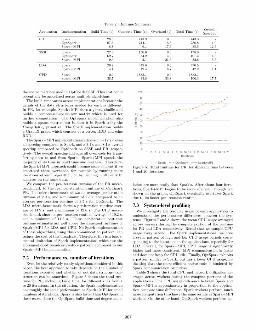
Table 2: Runtime Summary

Application Implementation Build Time (s) Compute Time (s) Overhead (s) Total Time (s)OverallSpeedup

PR Spark 28.8 413.9 0.6 443.3 -OptSpark 67.5 214.1 5.3 286.8 1.9Spark+MPI 8.8 9.1 17.6 35.5 12.5

SSSP Spark 27.8 150.6 0.6 178.9 -OptSpark 62.7 34.2 4.5 101.4 1.8Spark+MPI 9.0 2.1 21.6 32.6 5.5

LDA Spark 20.9 449.0 0.6 470.5 -Spark+MPI 4.1 19.4 18.7 42.2 11.1

CPD Spark 0.0 1883.1 0.0 1883.1 -Spark+MPI 38.7 33.8 33.8 106.3 17.7

the sparse matrices used in OptSpark SSSP. This cost couldpotentially be amortized across multiple algorithms.

The build time varies across implementations because thedetails of the data structures needed for each is different.In PR, for example, Spark+MPI does a global shuffle andbuilds a compressed-sparse-row matrix which is used forfurther computation. The OptSpark implementation alsobuilds a sparse matrix, but it does it in Spark using theGroupByKey primitive. The Spark implementation buildsa GraphX graph which consists of a vertex RDD and edgeRDD.

The Spark+MPI implementations achieve 5.5−17.7× over-all speedup compared to Spark, and a 3.1× and 8.1× overallspeedup compared to OptSpark on SSSP and PR, respec-tively. The overall speedup includes all overheads for trans-ferring data to and from Spark. Spark+MPI spends themajority of its time in build time and overhead. Therefore,the Spark+MPI approach could become more efficient if weamortized these overheads, for example by running moreiterations of each algorithm, or by running multiple MPIanalyses on the same data.

We compare the per-iteration runtime of the PR micro-benchmark to the real per-iteration runtime of OptSparkPR. The micro-benchmark shows an average per-iterationruntime of 2.9 s, and a minimum of 2.5 s, compared to anaverage per-iteration runtime of 3.5 s for OptSpark. TheLDA micro-benchmark shows a per-iteration runtime aver-age of 14.9 s, and a minimum of 12.6 s. The CPD micro-benchmark shows a per-iteration runtime average of 19.2 s,and a minimum of 14.6 s. These per-iteration best-caseruntime estimates are well above the measured runtimes ofSpark+MPI for LDA and CPD. No Spark implementationof these algorithms, using this communication pattern, canreduce the cost of this broadcast. Therefore, this is a funda-mental limitation of Spark implementations which use theaforementioned broadcast/reduce pattern, compared to ourSpark+MPI implementation.

7.2 Performance vs. number of iterationsEven for the relatively costly algorithms considered in this

paper, the best approach to take depends on the number ofiterations executed and whether or not data structure con-struction can be amortized. Figure 5 shows the total run-time for PR, including build time, for different runs from 1to 20 iterations. In this situation, the Spark implementationhas roughly the same performance as Spark+MPI for smallnumbers of iterations. Spark is also faster than OptSpark inthese cases, since the OptSpark build time and degree calcu-

0

20

40

60

80

100

120

140

160

180

200

1 2 3 4 5 6 7 8 9 10 11 12 13 14 15 16 17 18 19 20

Runtim

e (

s)

Iterations

Spark OptSpark Spark+MPI

Figure 5: Total runtime for PR, for different runs between1 and 20 iterations.

lation are more costly than Spark’s. After about four itera-tions, Spark+MPI begins to be more efficient. Though notshown on the graph, OptSpark eventually overtakes Sparkdue to its faster per-iteration runtime.

7.3 System­level profilingWe investigate the resource usage of each application to

understand the performance differences between the sys-tems. Figures 7 and 8 shows the mean CPU usage averagedacross workers during the compute portion of the runtimefor PR and LDA respectively. Recall that we sample CPUusage every second. For Spark implementations, we notea cyclic pattern of high and low CPU usage periods corre-sponding to the iterations in the applications, especially forLDA. Overall, for Spark+MPI, CPU usage is significantlyhigher and more consistent. MPI communication is fasterand does not keep the CPU idle. Finally, OptSpark exhibitsa pattern similar to Spark, but has a lower CPU usage, in-dicating that the more efficient native code is hindered bySpark communication primitives.

Table 3 shows the total CPU and network utilization av-eraged across workers during the compute portions of theapplications. The CPU usage difference between Spark andSpark+MPI is approximately in proportion to the applica-tion compute time difference. Spark workers perform muchmore computation to achieve the same results as Spark+MPIworkers. On the other hand, OptSpark workers perform ap-

907

0

5

10

15

20

25

30R

untim

e (

s)

Jobs

Algorithm Ser/Deser Sched. Delay Shuffle

Figure 6: Spark PR: Job profiling from Spark logs.

Spark+MPI

OptSpark

Spark

Figure 7: PR: CPU utilization of compute portion only.

Figure 8: LDA: CPU utilization of compute portion only.

Table 3: CPU and network total utilization during compute.

App System CPU (s) Network (Gbit)

LDA Spark 111 284Spark+MPI 11 431

PR Spark 61 481OptSpark 9 217Spark+MPI 9 282

SSSP Spark 21 70OptSpark 4 14Spark+MPI 2 33

CPD Spark 547 598Spark+MPI 23 105

proximately the same amount of computation as Spark+MPIworkers. Therefore, the compute time performance gap be-tween OptSpark and Spark+MPI is attributable to otherfactors, which we explore in Section 7.5.

7.4 Spark profileFigure 6 shows a breakdown of each job for PR in Spark,

computed with our log parser using data from Spark’s logs.There is one job per iteration, and the algorithm runs for54 iterations. The large runtimes for early jobs are likelybecause of data structure construction. For a typical itera-tion, the vast majority of the runtime is classified as algo-rithm time, which means time that is spent executing thetask. Algorithm time is distinct from scheduler overhead,serialization and deserialization time for the task, as well asshuffle time.

Though not shown here, the other applications have thesame property with respect to algorithm time. For PR,SSSP, LDA, and CPD, algorithm time accounts respectivelyfor 92%, 95%, 95%, and 91% of the total job time. We canrelate this with the results of system-level profiling in Sec-tion 7.3. These results show that during the compute por-tion, Spark implementations used significantly more overallCPU resources than either OptSpark or Spark+MPI imple-mentations. The logs suggest that, for Spark implementa-tions, these CPU cycles are spent inside of the Spark tasks.

Figure 9 is a screenshot from the Java Flight Recorderprofiler, showing the state of six threads (vertical axis) overtime (horizontal axis) running several iterations of PR onone cluster node. We observe load imbalance across threads;furthermore, we have noticed load imbalance across clusternodes from the logs (not depicted). We attribute the load

908

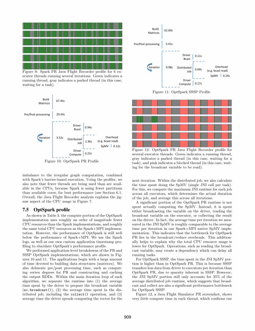
Figure 9: Spark PR Java Flight Recorder profile for 6 ex-ecutor threads running several iterations. Green indicates arunning thread, gray indicates a parked thread (in this case,waiting for a task).

Build

Matrices

Pre/Post-processing

Iteration

Driver

Bcast

Distributed

Job

Driver

Compute

SpMV

67.45s

29.43s

3.52s

0.94s

2.36s

0.22s

0.12s

Overhead

(e.g. bcast read)

Figure 10: OptSpark PR Profile

imbalance to the irregular graph computation, combinedwith Spark’s barrier-based execution. Using the profiler, wealso note that fewer threads are being used than are avail-able in the CPUs, because Spark is using fewer partitionsthan available cores, for best performance (see Section 6.1.Overall, the Java Flight Recorder analysis explains the jig-saw aspect of the CPU usage in Figure 7.

7.5 OptSpark profileAs shown in Table 3, the compute portion of the OptSpark

implementation uses roughly an order of magnitude fewerCPU resources than the Spark implementations, and roughlythe same total CPU resources as the Spark+MPI implemen-tation. However, the performance of OptSpark is still wellbelow the performance of Spark+MPI. We use the Sparklogs, as well as our own custom application timestamp pro-filing to elucidate OptSpark’s performance profile.

We performed application-level breakdowns of the PR andSSSP OptSpark implementations, which are shown in Fig-ures 10 and 11. The applications begin with a large amountof time devoted to building data structures (matrices). Wealso delineate pre/post processing time, such as comput-ing vertex degrees for PR and constructing and cachingthe output RDDs. Within the main iteration loop of eachalgorithm, we separate the runtime into (1) the averagetime spent by the driver to prepare the broadcast variable(sc.broadcast()), (2) the average time spent in the dis-tributed job, including the collect() operation, and (3)average time the driver spends computing the vector for the

Build

Matrices

Pre/Post-processing

Iteration

Driver

Bcast

Distributed

Job

Driver

Compute

SpMV

62.69s

5.41s

0.98s

0.11s

0.69s

0.17s

0.24s

Overhead

(e.g. bcast read)

Figure 11: OptSpark SSSP Profile

Figure 12: OptSpark PR Java Flight Recorder profile forseveral executor threads. Green indicates a running thread,gray indicates a parked thread (in this case, waiting for atask), and pink indicates a blocked thread (in this case, wait-ing for the broadcast variable to be read).

next iteration. Within the distributed job, we also calculatethe time spent doing the SpMV (single JNI call per task).For this, we compute the maximum JNI runtime for each jobacross all executors, which determines the actual durationof the job, and average this across all iterations.

A significant portion of the OptSpark PR runtime is notspent actually computing the SpMV. Instead, it is spenteither broadcasting the variable on the driver, reading thebroadcast variable on the executor, or collecting the resulton the driver. In fact, the average time per iteration we mea-sured in the JNI SpMV is roughly comparable to the averagetime per iteration in our Spark+MPI native SpMV imple-mentation. This indicates that the bottleneck for OptSparkPR lies in the broadcast/reduce overheads. This addition-ally helps to explain why the total CPU resource usage islower for OptSpark. Operations, such as reading the broad-cast variable, may create a dependency which can delay allrunning tasks.

For OptSpark SSSP, the time spent in the JNI SpMV por-tion is higher than in OptSpark PR. This is because SSSPtransfers less data from driver to executors per iteration thanOptSpark PR, due to sparsity inherent in SSSP. However,the JNI SpMV portion still only accounts for 35% of theaverage distributed job runtime, which suggests that broad-cast and collect are also a significant performance bottleneckfor OptSpark SSSP.

Figure 12, a Java Flight Simulator PR screenshot, showsvery little compute time in each thread, which confirms our

909

0

20

40

60

80

100

120

PR SSSP LDA CPD

Runtim

e (

s)

RDD to /dev/shm MPI to HDFS HDFS to RDD

Other Compute Time Build Time

Figure 13: Spark+MPI: Breakdown of the overheads in-curred when transferring data between Spark and MPI.

application profiling results in Figure 10. In Spark appli-cations, the broadcast variable is read by only one threadand the other threads are blocked during this time; this isrepresented in the pink in the figure. Note the short SpMVcomputation in each thread (green) after the broadcast vari-able is read. Gray indicates the results are being collectedby the driver, the driver is computing alone, or the driver ispreparing the next broadcast variable.

7.6 Spark+MPI profileFigure 13 shows a breakdown of total Spark+MPI run-

time, including overheads incurred when transferring databetween the Spark and MPI environments. PR and SSSPoverheads are almost identical because the sizes of the in-put graph and output data are roughly the same. However,the SSSP computation is much smaller so this means thatthe overheads are a much larger percentage of total SSSPruntime compared to PR. The time to transfer data fromSpark to shared memory, and from HDFS back into Spark,is roughly proportional to the size of the input and outputdata. The portion of time spent in compute ranges from aminimum of 6% (SSSP) to a maximum of 46% (LDA). Thisshow great potential for gains through repeated MPI com-putations in a pipeline, which would amortize the overheads.

7.7 Fault toleranceOne of the benefits of Spark is its ability to detect and

recover from faults. When one or more RDD partitions arediscovered to be missing, if the missing RDD partitions can-not be found in persistent storage, Spark is able to regener-ate them by examining the record of RDD transformationswhich generated the missing partitions and re-executing op-erations if necessary.

Since Spark+MPI performs operations outside of the Sparkenvironment, we can not rely entirely on Spark’s recoverymechanisms. Instead, we restart the entire Spark+MPIcomputation in response to a fault. We perform experimentsto quantify the performance cost of our approach comparedto Spark’s fault recovery for the same workload. We simu-late faults by killing the HDFS and Spark processes of oneof the cluster nodes after the last iteration of the algorithmcommences. This represents the worst-case fault timing.

Table 4: Fault recovery runtime for 10 iterations of PR onTwitter.

No fault (s) Restart (s) Recovery (s)

Spark 90.5 235.4 2461.6Spark+MPI 32.1 85.5 -

0

20

40

60

80

100

No Fault Fault

Ru

ntim

e (

s)

(10) Other

(9) HDFS to Spark

(8) MPI to HDFS

(7) Compute time

(6) Build time

(5) RDD to /dev/shm

(4) 10 second wait

(3) Compute time

(2) Build time

(1) RDD to /dev/shm

Figure 14: Spark+MPI PR runtime with restart after fault.

Table 4 shows the performance of Spark and Spark+MPIin the presence of the aforementioned fault for 10 iterationsof PR. No fault is the regular runtime without any fault.Restart is the runtime with a fault simulated by killing theHDFS and Spark processes and then restarting the compu-tation in the user code. Recovery is the time it takes Sparkto regenerate the output using lineage information, whichmeans we simulate the fault by killing processes, then callcount on the RDD which contained the output of PR. Thereis a 2.6× overall slowdown in Spark if you completely restartthe computation from the beginning, and a 27× slowdownfor relying on recovery from lineage. We therefore concludethat Spark libraries could benefit from application-level faultrecovery.

Figure 14 shows the runtime breakdown for Spark+MPIwhen there is no fault, and when there is a complete restartafter fault detection. The overall runtime is 2.7× higher inthe case of a fault compared to no fault. The runtime is bro-ken down into ten segments which occur chronologically: (1)Copying the RDD to shared memory for the first time, (2)building the graph data structure, (3) computing PR itera-tions, (4) 10 seconds of wait time while killing process, (5)Spark regenerating the input RDD after restart and copy-ing it to shared memory for the second time, (6) buildingthe graph data structure for the second time, (7) computingPR iterations for the second time, (8) writing the results toHDFS from MPI, (9) reading the results from HDFS intoSpark, and (10) time otherwise unaccounted for.

It takes much longer to copy the RDD after the fault,shown in segment (5), than before the fault. This is dueto Spark needing to regenerate the inputs from HDFS. Italso takes longer to (6) build data structures in MPI, and(7) compute in MPI during the second run. Since thereare only 11 compute nodes, a prime number, GraphMat isforced to use a 1D layout instead of the usual 2D layout,which hurts performance.

910

7.8 SummarySpark+MPI has runtime and memory overheads, which

depend on the size of input and the output of the oper-ation. Among our four application experiments, it takesbetween 3 − 5 seconds to transfer inputs to MPI throughshared memory, and between 9−19 seconds to transfer out-puts back into Spark through HDFS, plus between 4 − 8seconds of otherwise unaccounted time which may be re-lated to data transfer. By comparison, simple operations inSpark, such as count, can complete in one second or less onthe same datasets. Using Spark+MPI only makes sense foroperations which run slower in Spark than these fixed over-heads. Simple operations, such as scaling a vector stored inan RDD, should be done in Spark.

As long as there is enough work to amortize these fixedoverheads, applications can benefit from Spark+MPI. How-ever, some other applications may run with similar efficiencyin Spark, namely those which have less communication vol-ume and frequency. Since the main benefit of MPI is op-timized communication primitives, applications which havemore communication and more complex communication pat-terns will benefit relatively more from Spark+MPI.

8. CONCLUSIONSThere is a large gap between the efficiency of Spark and

MPI. This gap is exemplified by the variance in computetime we observed for Spark, OptSpark, and Spark+MPI.We sought to explain the nature of the gap by optimizingand profiling Spark to better understand its performance.The system we introduce in this paper, Spark+MPI, is asolution to bridging the gap, as proven quantitatively in ourevaluation on real applications and datasets.

In profiling Spark, we observed that the Spark implemen-tations consume a large amount of CPU resources comparedto OptSpark and Spark+MPI implementations. Further-more, the Spark logs tell us that, for the Spark implementa-tions, the time is being spent in algorithm time, running onthe executors. The OptSpark and Spark+MPI implemen-tations of PageRank show that the same algorithm can beimplemented using much fewer CPU cycles. Therefore, weconclude that the Spark implementations are making ineffi-cient use of CPU resources. At the same time, consideringOptSpark, we conclude that the performance of implementa-tions based on Spark’s communication primitives is greatlyimpeded by Spark’s broadcast and collect operations.

Despite its overheads, our Spark+MPI system providesbetter performance than the alternatives for the applica-tions and datasets considered in this paper. For algorithmswith fewer iterations, less work per iteration, or opportuni-ties to amortize data structure build times in Spark, it maybe more efficient to stay in Spark to avoid the overheads ofSpark+MPI. We demonstrated this by measuring PR run-times with different numbers of iterations. On the otherhand, finding larger chunks of work to do in MPI wouldmake it is even more advantageous to use our proposed sys-tem because the Spark+MPI overheads could be amortizedfurther.

In addition to overhead, another potential drawback of theSpark+MPI approach is that it must share memory withSpark. In this paper, we statically partition the memorybetween Spark and MPI, which is sufficient for these ap-plications. However, to accommodate MPI and Spark ap-

plications with more diverse memory requirements, we areconsidering for future work a mechanism to allow MPI toborrow memory from Spark.

We will release Spark+MPI as open-source software.

9. REFERENCES[1] D. C. Anastasiu and G. Karypis. L2knng: Fast exact

k-nearest neighbor graph construction with l2-normpruning. In Proceedings of the 24th ACMInternational Conference on Information andKnowledge Management, CIKM 2015, pages 791–800,New York, NY, USA, 2015. ACM.

[2] M. J. Anderson, N. Sundaram, N. Satish, M. M. A.Patwary, T. L. Willke, and P. Dubey. GraphPad:Optimized graph primitives for parallel anddistributed platforms. In 2016 IEEE InternationalParallel and Distributed Processing Symposium(IPDPS), pages 313–322, May 2016.

[3] A. Asuncion, M. Welling, P. Smyth, and Y. W. Teh.On smoothing and inference for topic models. InProceedings of the Twenty-Fifth Conference onUncertainty in Artificial Intelligence, UAI 2009, pages27–34, Arlington, Virginia, United States, 2009. AUAIPress.

[4] M. Axtmann, T. Bingmann, E. Jobstl, S. Lamm,H. C. Nguyen, A. Noe, M. Stumpp, P. Sanders,S. Schlag, and T. Sturm. Thrill - distributed big databatch processing framework in C++.http://project-thrill.org/, 2016.

[5] D. M. Blei, A. Y. Ng, and M. I. Jordan. LatentDirichlet allocation. J. Mach. Learn. Res., 3:993–1022,Mar. 2003.

[6] R. Bosagh Zadeh, X. Meng, A. Ulanov, B. Yavuz,L. Pu, S. Venkataraman, E. Sparks, A. Staple, andM. Zaharia. Matrix computations and optimization inApache Spark. In Proceedings of the 22nd ACMSIGKDD International Conference on KnowledgeDiscovery and Data Mining, KDD 2016, pages 31–38,New York, NY, USA, 2016. ACM.

[7] deeplearning4j. Deep Learning for Java. Open-Source,Distributed, Deep Learning Library for the JVM.http://deeplearning4j.org/, 2016.

[8] G. E. Fagg and J. J. Dongarra. FT-MPI: Faulttolerant MPI, supporting dynamic applications in adynamic world. In Recent Advances in Parallel VirtualMachine and Message Passing Interface(EuroPVM/MPI), pages 346–353. Springer Nature,2000.

[9] M. P. I. Forum. Mpi: A message-passing interfacestandard version 3.1. Technical report, 2015.

[10] M. Gamell, D. S. Katz, H. Kolla, J. Chen, S. Klasky,and M. Parashar. Exploring automatic, online failurerecovery for scientific applications at extreme scales.In International Conference for High PerformanceComputing, Networking, Storage and Analysis. IEEE,2014.

[11] A. Gittens, A. Devarakonda, E. Racah,M. Ringenburg, L. Gerhardt, J. Kottalam, J. Liu,K. Maschhoff, S. Canon, J. Chhugani, P. Sharma,J. Yang, J. Demmel, J. Harrell, V. Krishnamurthy,M. W. Mahoney, and Prabhat. Matrix factorizationsat scale: A comparison of scientific data analytics in

911

Spark and C+MPI using three case studies. In 2016IEEE International Conference on Big Data (BigData), pages 204–213, Dec 2016.

[12] M. Grossman and V. Sarkar. SWAT: Aprogrammable, in-memory, distributed,high-performance computing platform. InInternational Symposium on High-PerformanceParallel and Distributed Computing (HPDC), pages81–92, New York, New York, USA, 2016. ACM Press.

[13] H2O.ai. Sparkling Water.https://github.com/h2oai/sparkling-water, 2016.

[14] S. Jha, J. Qiu, A. Luckow, P. Mantha, and G. C. Fox.A tale of two data-intensive paradigms: Applications,abstractions, and architectures. In IEEE InternationalCongress on Big Data. IEEE, 2014.

[15] O. Kaya and B. Ucar. Scalable sparse tensordecompositions in distributed memory systems. InProceedings of the International Conference for HighPerformance Computing, Networking, Storage andAnalysis, page 77. ACM, 2015.

[16] T. G. Kolda and B. Bader. The TOPHITS model forhigher-order web link analysis. In Proceedings of LinkAnalysis, Counterterrorism and Security 2006, 2006.

[17] T. G. Kolda and B. W. Bader. Tensor decompositionsand applications. SIAM review, 51(3):455–500, 2009.

[18] H. Kwak, C. Lee, H. Park, and S. B. Moon. What isTwitter, a social network or a news media? In WWW,pages 591–600, 2010.

[19] X. Lu, F. Liang, B. Wang, L. Zha, and Z. Xu.Datampi: Extending MPI to Hadoop-like big datacomputing. In 28th IEEE International Parallel andDistributed Processing Symposium, pages 829–838,May 2014.

[20] J. McAuley and J. Leskovec. Hidden factors andhidden topics: understanding rating dimensions withreview text. In Proceedings of the 7th ACM conferenceon recommender systems, pages 165–172. ACM, 2013.

[21] X. Meng, J. Bradley, B. Yavuz, E. Sparks,S. Venkataraman, D. Liu, J. Freeman, D. Tsai,M. Amde, S. Owen, D. Xin, R. Xin, M. J. Franklin,R. Zadeh, M. Zaharia, and A. Talwalkar. MLlib:Machine learning in Apache Spark. J. Mach. Learn.Res., 17(1):1235–1241, Jan. 2016.

[22] K. Ousterhout, R. Rasti, S. Ratnasamy, S. Shenker,and B.-G. Chun. Making sense of performance in dataanalytics frameworks. In Proceedings of the 12thUSENIX Conference on Networked Systems Designand Implementation, NSDI 2015, pages 293–307,Berkeley, CA, USA, 2015. USENIX Association.

[23] A. Raveendran, T. Bicer, and G. Agrawal. Aframework for elastic execution of existing MPIprograms. In IEEE International Symposium onParallel and Distributed Processing Workshops andPhD Forum (IPDPSW), pages 940–947, May 2011.

[24] J. L. Reyes-Ortiz, L. Oneto, and D. Anguita. Big data

analytics in the cloud: Spark on Hadoop vsMPI/OpenMP on Beowulf. Procedia ComputerScience, 53:121 – 130, 2015.

[25] N. Satish, N. Sundaram, M. M. A. Patwary, J. Seo,J. Park, M. A. Hassaan, S. Sengupta, Z. Yin, andP. Dubey. Navigating the maze of graph analyticsframeworks using massive graph datasets. InProceedings of the 2014 ACM SIGMOD InternationalConference on Management of Data, SIGMOD 2014,pages 979–990, New York, NY, USA, 2014. ACM.

[26] Y. Shi, A. Karatzoglou, L. Baltrunas, M. Larson,A. Hanjalic, and N. Oliver. TFMAP: optimizing mapfor top-n context-aware recommendation. InProceedings of the 35th International ACM SIGIRconference on Research and development ininformation retrieval, pages 155–164. ACM, 2012.

[27] N. D. Sidiropoulos, L. De Lathauwer, X. Fu,K. Huang, E. E. Papalexakis, and C. Faloutsos. Tensordecomposition for signal processing and machinelearning. arXiv preprint arXiv:1607.01668, 2016.

[28] G. M. Slota, S. Rajamanickam, and K. Madduri. Acase study of complex graph analysis in distributedmemory: Implementation and optimization. In 2016IEEE International Parallel and DistributedProcessing Symposium (IPDPS), pages 293–302, May2016.

[29] S. Smith, J. W. Choi, J. Li, R. Vuduc, J. Park, X. Liu,and G. Karypis. FROSTT: The formidable repositoryof open sparse tensors and tools, 2017.

[30] S. Smith and G. Karypis. SPLATT: The SurprisinglyParalleL spArse Tensor Toolkit.http://cs.umn.edu/~splatt/.

[31] S. Smith and G. Karypis. A medium-grainedalgorithm for distributed sparse tensor factorization.In 30th IEEE International Parallel & DistributedProcessing Symposium (IPDPS 2016), 2016.

[32] N. Sundaram, N. Satish, M. M. A. Patwary, S. R.Dulloor, M. J. Anderson, S. G. Vadlamudi, D. Das,and P. Dubey. GraphMat: High performance graphanalytics made productive. Proc. VLDB Endow.,8(11):1214–1225, July 2015.

[33] R. S. Xin, J. E. Gonzalez, M. J. Franklin, andI. Stoica. GraphX: A resilient distributed graphsystem on Spark. In First International Workshop onGraph Data Management Experiences and Systems,GRADES 2013, pages 2:1–2:6, New York, NY, USA,2013. ACM.

[34] M. Zaharia, M. Chowdhury, T. Das, A. Dave, J. Ma,M. McCauley, M. J. Franklin, S. Shenker, andI. Stoica. Resilient distributed datasets: Afault-tolerant abstraction for in-memory clustercomputing. In Proceedings of the 9th USENIXConference on Networked Systems Design andImplementation, NSDI 2012, pages 2–2, Berkeley, CA,USA, 2012. USENIX Association.

912