Brainstorm: Manic Depression, OccupationalChoice And Creativity

Carol Horton Tremblay,* Shawna Grosskopfand

Ke YangDepartment of Economics

Ballard Extension Hall 303Oregon State University

Corvallis, OR 97331-3612∗

This version: May 2004

∗We gratefully acknowledge helpful comments from James F. Ragan, Jr., Victor J.Tremblay and the participants at the SEA meetings in Tampa FL, 2001. We thank Ado-nis Yatchew for encouraging us not to give up on density estimation. Please relay allcorrespondence to Carol Horton Tremblay at the address above or by phone: (541) 737-1468, FAX: (541) 737-5917, or e-mail: CTremblay@oregonstate.edu.

1

Brainstorm: Manic Depression, Occupational Choice AndCreativity

Abstract

Although economists have analyzed earnings, unemployment, and laborforce participation for manic-depressives, occupational choice has yet to beexplored. There are psychiatric case studies focusing on occupational cre-ativity, but they likely suffer from selection bias. We employ two population-based data sets and estimate a multinomial logit model of occupational out-comes matched to a measure of occupational creativity. Manic-depressivesappear to be disproportionately concentrated in the most creative occupa-tional category, which we confirm by estimating nonparametric kernel den-sities of occupational creativity for bipolar and non-bipolar samples. Wefind significant differences; the probability of employment in creative jobs ishigher for bipolar than non-bipolar workers.

2

1 Introduction

If a man comes to the door of poetry untouched by the madness ofthe Muses, believing that technique alone will make him a goodpoet, he and his sane compositions never reach perfection, butare utterly eclipsed by the performances of the inspired madman.

Socrates1

The hypothesized association between creativity and manic-depressiveillness is an age-old controversy.2 Manic depression or bipolar illness is char-acterized by pronounced mood swings—alternating periods of elation, nor-malcy, and despondency, which can be accompanied by hallucinations ordelusions during the peaks and troughs of the cycles. Although we mightexpect bipolar illness to hamper occupational and artistic achievement, thecreativity and energy characteristic of persons with mania may actually im-prove their labor market outcomes (Frank and McGuire, 2000).

There is a fair amount of economics literature regarding mental illnessin general and in the labor market. As might be expected, research on thementally ill as a group has shown that they earn less than the well on aver-age, all else equal (Bartel and Taubman, 1979, 1986; Benham and Benham,1982, with the exception of neurotics; Frank and Gertler, 1991, for two ofthree measures of mental illness). Further, even when accounting for endo-geneity, the mentally ill are less likely to be employed (Hamilton et al., 1997).

Following Bartel and Taubman (1986), who emphasized the importanceof distinguishing among types of mental illness in economic analysis, theliterature began to focus on more specific illnesses. Regarding the class of af-fective disorders (manic-depressive and unipolar depressive illnesses), Millerand Kelman (1992) find that affective illness is positively associated with in-come, but disclaim their results due to selection bias. Focusing on unipolardepression, Berndt et al. (1998) show that depression lowers perceived workperformance.

1Plato (1974 translation).2See Jamison (1993) for a thorough history and literature review of the topic.

3

Turning to those with bipolar illness, there are about 2.3 million Amer-ican adults, or 1.2 percent of the population, who have manic-depressiveillness (Weissman et al., 1991). The employment rate of manic-depressivesis approximately 71 percent compared to about 82 percent for the generalpopulation, and manic-depressives earn about 57 percent of the earnings ofothers, all else equal (Ettner et al., 1997). In contrast to poorer employmentand earnings outcomes in the Ettner et al. (1997) study, Marcotte et al.(2000) find that bipolar status in the past year does not significantly affectincome or employment for men or women, but that length of time with abipolar disorder positively and significantly affects employment for women.Further, the lifetime number of bipolar episodes appears to significantly in-crease income for men. These mixed findings for the bipolar populationsuggest a need for further study.

None of the economic studies to date have addressed the issue of occu-pational outcomes for those with manic-depressive illnesses. Yet there is asubstantial body of research on the possible link between creative and artis-tic occupations and manic-depressive illness in the medical and behavioralsciences literature. About 75% of these studies find evidence of such a link(Jamison, 1993). Much of this research derives from case studies, biographiesof prominent historical figures in the arts, or diagnostic and psychologicalstudies of living writers, artists, and composers. Although rich and informa-tive in their own right, these studies may suffer from small sample sizes orfrom selection bias. For example, biographers likely do not choose their sub-jects at random. Manic-depressives may be more interesting and colorful towriters and to readers, and if so, focusing on biography subjects may resultin an erroneous apparent correlation between the illness and artistic ability.In addition, researchers may over- or under-diagnose bipolar disorder amongcreative figures, being influenced by the prominence of the hypothesis at thetime.

We use two samples: the first is a large population-based sample withautomated implementation of the diagnostic criteria to distinguish manic-depressives from the rest of the sample, the second is also a large population-based sample but with self reported diagnosis of bipolar illness. These shouldhelp to avoiding small sample and selection biases. Our goal here is to exam-ine the link between manic depression and occupation by estimating a tradi-tional economic model of occupational outcomes, namely a multinomial logit

4

model of occupational choice. We also investigate whether manic-depressivesare concentrated in more creative occupations based on nonparametric den-sity estimation.

The general outline of the paper is as follows. We begin with a briefdescription of manic depression and some of the issues related to occupa-tional choice and outcome for those diagnosed as bipolar. We turn next to adiscussion of our data sets, the Epidemiologic Catchment Area (ECA) dataset and the Mental Health Supplement (MHS) of the National Health Inter-view Survey, which we employ to provide evidence concerning occupationalchoice and the “creativity” of the occupation based on a measure from theDictionary of Occupational Titles. After discussing our multinomial logitresults, we turn to additional evidence based on nonparametric estimationtechniques and other forms of manic-depressive illness.

2 The Nature of Manic Depression and its

Relation to Creativity

And Something’s odd withinThat person that I wasAnd this One do not feel the sameCould it be Madness this?

Emily Dickinson

The expression of manic-depressive illness varies considerably across indi-viduals and over time for a given individual. There is a spectrum of severityof symptoms, both on the depressive and manic side, and considerable varia-tion in the age of onset, presence and severity of hallucinations and delusions,and the frequency, duration, and pattern of manic, depressive, and normalepisodes. For example, in a recent study, Post et al. (2003) follow the dailycourse of illness for 258 bipolar outpatients for one year. They find that evenwith state-of-the-art medications, 26.4 percent spent at least 9 months of theyear in a manic or depressive state. An additional 40.7 percent were episodi-cally ill, while 32.9 percent of the patients were minimally impaired over the

5

year. This sample probably overstates the severity of illness of the bipolarpopulation since these patients were at “treatment centers with a record ofexcellence” which may draw an over-representation of people with particu-larly severe or treatment-resistant illness. Those who are functioning welldo not usually seek help, and those with manageable symptoms are readilytreated by local psychiatrists.3

The clinical definition of mania may help to clarify the meaning of manicdepression. Depression characterizes both unipolar and bipolar illness; thusit is an episode of mania that distinguishes manic depression (or bipolar Idisorder) from unipolar illness. Detailed symptoms of mania are includedin the first column of appendix table A.1, but generally speaking, a manicepisode entails “a distinct period of abnormally and persistently elevated,expansive or irritable mood,” which may alternate with depressive mood. Amanic episode is characterized by at least three of the following symptoms:increased activity, talkativeness, flight of ideas, inflated self-esteem, decreasedneed for sleep, distractibility, and excessive involvement in risky activities.Physiological evidence of manic phases are displayed in Illustration 1 of brainscans of a patient during manic and depressive phases, which is reproducedfrom Goodwin and Jamison (1990, p. 458b).

The aforementioned list of symptoms provides some motivation for thelink between the disorder and creativity. For example “flight of ideas” evokesimages of poets, writers or musicians in the throes of creativity. The “talka-tiveness” feature enables some manic-depressives to easily and fluently vo-calize rhymes and formulate word associations, facilitating the writing ofpoetry and verse (Jamison, 1993). Increased activity and decreased need forsleep may bolster productivity in a number of occupations. As an example,Illustration 2 (reproduced from Goodwin and Jamison, 1990, p.348) tracksthe career history of the composer Robert Schumann. The numbers on theIllustration identify each opus written in each year, while the lower portionindicates the psychiatric diagnosis4 and suicide attempts. The cyclical pat-tern of Schumann’s work and its correspondence with his psychiatric state is

3Post el al. argue that daily participation in the project requires motivation and com-

mitment which may counter the selection bias discussed above. It may be however, that

those who are most impaired have the greatest to gain from participation in the study.4Hypomania is a mild, non-psychotic, form of mania.

6

striking. On the other hand, many of the symptoms of mania listed above,such as distractibility, would typically be associated with reduced effective-ness in virtually any occupation.

Because they experience the height and depth of emotion, manic-depressivesmay be able to produce rich and moving poetry, art, and music to a greaterextent than if they were well. Additionally, the disease may drive manic-depressives to use artistic expression to soothe their turmoil. Perhaps cre-ative persons are prone to manic depression due to genetic factors. Unaf-flicted close relatives of bipolars tend to be more creative than the generalpopulation (Jamison, 1993), suggesting that there is a genetic link betweenthe illness and creativity. We do not presume to disentangle these potentialcausal factors here, but attempt to first establish whether or not there is anassociation between manic depression and occupational creativity.

3 Data and Methods

The main dataset we utilize is the Epidemiologic Catchment Area Study(ECA), collected by researchers at Yale University, Johns Hopkins Univer-sity, Washington University, Duke University and University of California atLos Angeles in collaboration with the National Institute of Mental Health(NIMH; U.S. Department of Health and Human Services, 1994). Data wereobtained by personal interviews of 20,861 adults residing in the communitiesof these universities: New Haven, Baltimore, St. Louis, Durham and LosAngeles. Respondents were selected using multistage probability sampling.We use the most recent wave of the survey, Wave II, which was collected in1981-1985.

To determine if an individual meets the criteria for having a particularmental illness, the ECA interviewers elicited responses to the NIMH Diagnos-tic Interview Schedule (DIS). Questions are designed to identify symptomscorresponding to criteria in the Diagnostic and Statistical Manual of MentalDisorders, third edition (DSM-III; American Psychiatric Association, 1980).Appendix Table A.1 compares the DSM-III criteria to the corresponding DISquestions for the diagnosis of mania. Once the DIS responses are entered intoa data file, the DSM-III criteria are operationalized by computer, and diag-

7

noses are generated for mania as well as a number of other mental illnesses.The fraction of the sample with a DSM-III manic episode diagnosis is 0.62.5

We also consider an alternative diagnostic criteria, the 1987 revised ver-sion of the DSM-III, abbreviated DSM-III-R. In addition to the mania diag-nosis requirements in the DSM-III, the DSM-III-R includes the criterion ofhospitalization or marked impairment in occupational functioning or usualsocial activities. Excluding those who do not meet this severity criterion, re-duces the number of individuals with a DSM-III-R manic episode diagnosisto a total of 46 or 0.34 percent of the sample.

To supplement the ECA results, we consider information from anotherdata source: the National Health Interview Survey, 1989: Mental HealthSupplement (MHS).6 Rather than using the DSM-III or DSM-III-R criteriato identify bipolar illness in the sample, the MHS identifies manic depressionby simply asking the respondent in the interview whether or not he or shehas had the disease in the past 12 months. Thus, the reference is in thelast 12 months rather than lifetime as in the ECA data, and the diagnosisis self-reported rather than identified based on identification of symptoms asin the ECA. We would expect that those identified as bipolars in the MHSwould typically be more severely impaired than those identified as bipolar inthe ECA study.

Both the ECA and MHS samples also contain occupational codes. Table

5Individuals who have had a manic episode but experienced psychotic symptoms before

or independent of an episode or who have an organic brain disorder are excluded from the

mania diagnosis.6In a preliminary draft of this paper, we also made use of the National Comorbidity

Survey (NCS), 1990-1992 (Kessler, 2002). We are concerned about the NCS mania diagno-

sis (Kessler, 2001), however, and will await the release of the new NCS surveys in July 2004

for future work (Harvard, 2003). Originally, the NCS diagnosis was tied to DSM-III-R but

was found to over-diagnose manic depression. The criteria were adjusted and appear to be

free of generating false positives, but now they under-diagnose manic depression relative

to generally accepted rates of prevalence. We understand that improvements in diagnosis

are in place for the upcoming NCS surveys (Kessler, 2001).

8

1 lists the percent of employment in each major occupational group by manicepisode status for our two samples and the two forms of bipolar diagnosisin the ECA sample (DSM-III and DSM-III-R). There is a greater represen-tation of those with a bipolar I diagnosis than the rest of the populationemployed in the managerial and professional occupations and services basedon the ECA sample data, but not in the MHS data. In both the ECA andMHS samples, bipolars are relatively ‘overrepresented’ in the services. In theMHS data bipolars are most highly concentrated in the technical, sales andclerical category. The occupational segregation index (Duncan and DuncanIndex of Occupational Dissimilarity) corresponding to the figures in Table1 for the ECA sample is 13.3, indicating that identical occupation distribu-tions for manic-depressives and those with no history of mania would ariseif 13.3 percent of either group changed occupations for bipolar DSM-IIIs .To put this figure in perspective, note that it equals the value of the occu-pational segregation index for African and white American women in 1995(Blau et al., 1998). The estimated occupational segregation index for DSM-III-R bipolars relative to the well is 18.7 percent, higher than for the bipolarsdiagnosed under the less restrictive DSM-III criteria. For the MHS samplethe occupational segregation index is 17.23.

To measure creativity for each individual, we use occupation creativityscores from England and Kilbourne (1988) matched to individuals by 3-digit occupation codes. The occupational creativity measure represents thepercentage of employees in a particular occupation who engage in abstractand creative activities. Examples of abstract and creative activities include:painting, hairstyling, writing, music teaching, interpreting public opinionsurveys in light of contemporary society, creating dramatic stage lighting,planning advertising campaigns, and diagnosing illness (U.S. Department ofLabor, 1972).

Table 2 shows that the mean and median values of the occupationalcreativity index vary substantially by occupation group.7 Managerial andprofessional occupations have the highest mean and median creativity levelrelative to the other occupational groups, and based on the ECA sample, thisoccupational category employs an ‘over-representation’ of those with manicdepression, as shown in Table 1. Further, the managerial and professional

7These statistics are based on bipolar and non-bipolar individuals.

9

occupational group includes all of the 3-digit occupations classified by Filer(1986) as “artistic.”8 In the services, where manic-depressives are also over-represented (see Table 1), the extent of creativity is less clear. Taking a moredirect approach, we segment the sample by diagnosis status and compute theoccupational creativity index. For the ECA sample, we find that both themean and median values of the occupational creativity index are higher formanic-depressive DSM-IIIs and DSM-III-Rs (means = 4.35 and 4.54, medi-ans = 0.46 and 0.38) than by those not so afflicted (mean = 3.07, median =0.12). Also included in Table 2 are data for those who are classified as bipolarII. Bipolar II is a bipolar disorder with more moderate manic episodes thanbipolar I disorder; they more closely resemble the non-bipolar population interms of the mean and median creativity indexes as one might expect. Fi-nally the results for the bipolar I population in the MHS data set suggestthat mean and median creativity indexes are higher in the non-bipolar pop-ulation, although the differences are small.

We explore one other measure of creativity from the psychology and careercounseling literature: the Holland Artistic (A) Occupational Code (Gottfred-son and Holland, 1996).9 We merged the Holland codes to our ECA sample

8These include actors and directors; authors; dancers; designers working in the theater,

motion pictures, or art museums; musicians and composers; painters, sculptors, craft

artists, and artistic printmakers; photographers; postsecondary teachers of art, drama and

music; and artists, performers and related workers not elsewhere classified.9According to Gottfredson and Holland (p. 2), the Artistic occupational environment

“requires innovation or creative ability. It rewards the display of imagination in artis-

tic, literary, or musical accomplishments, and allows the expression of unconventional

ideas or manners. Occupations classified as Artistic generally involve creative work in the

arts: music, writing, performance, sculpture, or other relatively unstructured and intellec-

tual endeavors.” The Holland model classifies five additional occupational environments:

Realistic (R, e.g. carpenter or truck operator), Investigative (I, e.g. psychologist or mi-

crobiologist), Social (S, e.g. counselor or clergy member), Enterprising (E, e.g. lawyer

or retail store manager), and Conventional (C, e.g. production editor, bookkeeper). For

seven different occupational coding systems, Gottfredson and Holland assign three of the

six categories, in descending order of importance, to each occupation. For example, the

10

by 3-digit occupational code, and we used the DSM-III criteria to distin-guish manic-depressives from others in the merged sample. We find thatthe percent of individuals who are employed in occupations with an Artisticcomponent is greater for the bipolar group, 10.71 percent, than for the non-bipolar group, 8.40 percent. The small sample of bipolar individuals, 75 inthe non-artistic occupations and only 9 in the artistic occupations, limit theweight of this evidence.

In the next section we turn to traditional empirical models used in eco-nomics to analyze occupational choice. Specifically we use multinomial logitestimation of occupational choice to determine if bipolar status significantlyaffects occupational choice. We then return to analyzing the relationshipbetween manic depression and the occupational creativity index. The largedifferences between the mean and median values of the index, displayed inTable 2, indicate that the distribution is highly skewed. Thus, parametrictechniques may not be appropriate, particularly since the distribution is un-known. Consequently, we use kernel density estimation and nonparametrichypothesis tests to explore potential differences in the occupational creativityindex densities for manic-depressives and for other individuals.

4 Results

4.1 Multinomial Logit Occupation Regressions

In what follows, we estimate a multinomial logit model of the probabilityof employment in each occupational group as a function of bipolar I sta-tus. Control variables in the base model include RACE = 1 if individual i isAfrican-American (= 0 otherwise), FEM = 1 if i is female (= 0 otherwise),MARRIED = 1 if i is presently married (= 0 otherwise), and AGE. Sets of

code for economists is ISA, investigative rated most important, followed by social (which

includes teaching, mentoring and concern for the welfare of others), and then artistic

(likely for the creativity and innovation features). The statistics referred to above apply

to all occupations that have an Artistic component (i.e., Axx, xAx, or xxA where x = R,

I, S, E, C).

11

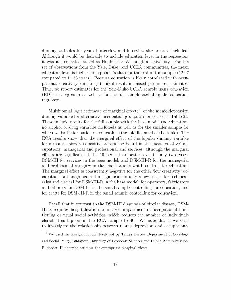
dummy variables for year of interview and interview site are also included.Although it would be desirable to include education level in the regression,it was not collected at Johns Hopkins or Washington University. For theset of observations from the Yale, Duke, and UCLA communities, the meaneducation level is higher for bipolar I’s than for the rest of the sample (12.97compared to 11.53 years). Because education is likely correlated with occu-pational creativity, omitting it might result in biased parameter estimates.Thus, we report estimates for the Yale-Duke-UCLA sample using education(ED) as a regressor as well as for the full sample excluding the educationregressor.

Multinomial logit estimates of marginal effects10 of the manic-depressiondummy variable for alternative occupation groups are presented in Table 3a.These include results for the full sample with the base model (no education,no alcohol or drug variables included) as well as for the smaller sample forwhich we had information on education (the middle panel of the table). TheECA results show that the marginal effect of the bipolar dummy variablefor a manic episode is positive across the board in the most ‘creative’ oc-cupations: managerial and professional and services, although the marginaleffects are significant at the 10 percent or better level in only two cases:DSM-III for services in the base model, and DSM-III-R for the managerialand professional category in the small sample which controls for education.The marginal effect is consistently negative for the other ‘low creativity’ oc-cupations, although again it is significant in only a few cases: for technical,sales and clerical for DSM-III-R in the base model; for operators, fabricatorsand laborers for DSM-III in the small sample controlling for education; andfor crafts for DSM-III-R in the small sample controlling for education.

Recall that in contrast to the DSM-III diagnosis of bipolar disease, DSM-III-R requires hospitalization or marked impairment in occupational func-tioning or usual social activities, which reduces the number of individualsclassified as bipolar in the ECA sample to 46. We note that if we wishto investigate the relationship between manic depression and occupational

10We used the margin module developed by Tamas Bartus, Department of Sociology

and Social Policy, Budapest University of Economic Sciences and Public Administration,

Budapest, Hungary to estimate the appropriate marginal effects.

12

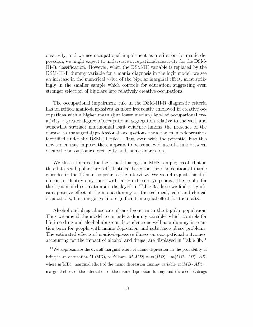
creativity, and we use occupational impairment as a criterion for manic de-pression, we might expect to understate occupational creativity for the DSM-III-R classification. However, when the DSM-III variable is replaced by theDSM-III-R dummy variable for a mania diagnosis in the logit model, we seean increase in the numerical value of the bipolar marginal effect, most strik-ingly in the smaller sample which controls for education, suggesting evenstronger selection of bipolars into relatively creative occupations.

The occupational impairment rule in the DSM-III-R diagnostic criteriahas identified manic-depressives as more frequently employed in creative oc-cupations with a higher mean (but lower median) level of occupational cre-ativity, a greater degree of occupational segregation relative to the well, andsomewhat stronger multinomial logit evidence linking the presence of thedisease to managerial/professional occupations than the manic-depressivesidentified under the DSM-III rules. Thus, even with the potential bias thisnew screen may impose, there appears to be some evidence of a link betweenoccupational outcomes, creativity and manic depression.

We also estimated the logit model using the MHS sample; recall that inthis data set bipolars are self-identified based on their perception of manicepisodes in the 12 months prior to the interview. We would expect this def-inition to identify only those with fairly extreme symptoms. The results forthe logit model estimation are displayed in Table 3a; here we find a signifi-cant positive effect of the mania dummy on the technical, sales and clericaloccupations, but a negative and significant marginal effect for the crafts.

Alcohol and drug abuse are often of concern in the bipolar population.Thus we amend the model to include a dummy variable, which controls forlifetime drug and alcohol abuse or dependence as well as a dummy interac-tion term for people with manic depression and substance abuse problems.The estimated effects of manic-depressive illness on occupational outcomes,accounting for the impact of alcohol and drugs, are displayed in Table 3b.11

11We approximate the overall marginal effect of manic depression on the probability of

being in an occupation M (MD), as follows: M(MD) ' m(MD) + m(MD · AD) · AD,

where m(MD)=marginal effect of the manic depression dummy variable, m(MD · AD) =

marginal effect of the interaction of the manic depression dummy and the alcohol/drugs

13

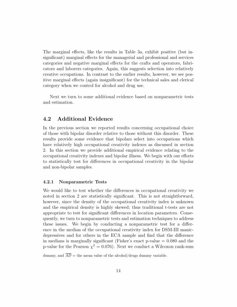
The marginal effects, like the results in Table 3a, exhibit positive (but in-significant) marginal effects for the managerial and professional and servicescategories and negative marginal effects for the crafts and operators, fabri-cators and laborers categories. Again, this suggests selection into relativelycreative occupations. In contrast to the earlier results, however, we see pos-itive marginal effects (again insignificant) for the technical sales and clericalcategory when we control for alcohol and drug use.

Next we turn to some additional evidence based on nonparametric testsand estimation.

4.2 Additional Evidence

In the previous section we reported results concerning occupational choiceof those with bipolar disorder relative to those without this disorder. Theseresults provide some evidence that bipolars select into occupations whichhave relatively high occupational creativity indexes as discussed in section2. In this section we provide additional empirical evidence relating to theoccupational creativity indexes and bipolar illness. We begin with our effortsto statistically test for differences in occupational creativity in the bipolarand non-bipolar samples.

4.2.1 Nonparametric Tests

We would like to test whether the differences in occupational creativity wenoted in section 2 are statistically significant. This is not straightforward,however, since the density of the occupational creativity index is unknownand the empirical density is highly skewed; thus traditional t-tests are notappropriate to test for significant differences in location parameters. Conse-quently, we turn to nonparametric tests and estimation techniques to addressthese issues. We begin by conducting a nonparametric test for a differ-ence in the median of the occupational creativity index for DSM-III manic-depressives and for others in the ECA sample and find that the differencein medians is marginally significant (Fisher’s exact p-value = 0.080 and thep-value for the Pearson χ2 = 0.076). Next we conduct a Wilcoxon rank-sum

dummy, and AD = the mean value of the alcohol/drugs dummy variable.

14

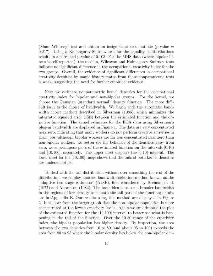
(Mann-Whitney) test and obtain an insignificant test statistic (p-value =0.217). Using a Kolmogorov-Smirnov test for the equality of distributionsresults in a corrected p-value of 0.103. For the MHS data (where bipolar ill-ness is self-reported), the median, Wilcoxon and Kolmogorov-Smirnov testsindicate no significant difference in the occupational creativity index for thetwo groups. Overall, the evidence of significant differences in occupationalcreativity densities by manic history status from these nonparametric testsis weak, suggesting the need for further empirical evidence.

Next we estimate nonparametric kernel densities for the occupationalcreativity index for bipolar and non-bipolar groups. For the kernel, wechoose the Gaussian (standard normal) density function. The more diffi-cult issue is the choice of bandwidth. We begin with the automatic band-width choice method described in Silverman (1986), which minimizes theintegrated squared error (ISE) between the estimated function and the ob-jective function. The kernel estimates for the ECA data using Silverman’splug-in bandwidth are displayed in Figure 1. The data are very concentratednear zero, indicating that many workers do not perform creative activities intheir jobs, although bipolar workers are far less concentrated near zero thannon-bipolar workers. To better see the behavior of the densities away fromzero, we superimpose plots of the estimated function on the intervals [0,10)and [10,100], separately. The upper inset displays the [0,10) interval. Thelower inset for the [10,100] range shows that the tails of both kernel densitiesare undersmoothed.

To deal with the tail distribution without over smoothing the rest of thedistribution, we employ another bandwidth selection method known as the‘adaptive two stage estimator’ (A2SE), first considered by Breiman et al.(1977) and Abramson (1982). The basic idea is to use a broader bandwidthin the regions of low density to smooth the tail part of the function; detailsare in Appendix B. Our results using this method are displayed in Figure2. It is clear from the larger graph that the non-bipolar population is moreconcentrated at the lowest creativity levels. Again we superimpose the plotof the estimated function for the [10,100] interval to better see what is hap-pening in the tail of the function. Over the 10-80 range of the creativityindex, the bipolar population has higher density. By inspection, the areabetween the two densities from 10 to 80 (and about 95 to 100) exceeds thearea from 80 to 95 where the bipolar density lies below the non-bipolar den-

15

sity. Next we present values of the tail probabilities for alternate values ofthe occupational creativity index.

To better see what is going on in the tails, we calculate the probabilitiesof observing the occupational creativity index above various values (integers1 through 10) for each group. These are displayed in Table 4. Recall thatthe median level of the occupational creativity index (c) lies between 0.12and 0.46 for the ECA bipolar and non-bipolar samples, respectively (see Ta-ble 2b). The probability that c is greater than or equal to one in column(1) represents part of the “tail” above the median. For the ECA data wesee that the probability of observing an occupational creativity index greaterthan one is higher for bipolars than non-bipolars (.3095 versus .2599). Theprobability is higher for bipolars for every value of the creativity index up togreater than or equal to 10, which represents 4-7 percent of the samples.

To test if these densities are significantly different, we follow the methodproposed by Li (1996). Let the two densities be f(x) and g(x), then test thenull hypothesis Ho : f(x) = g(x) against H1 : f(x) 6= g(x). The idea is toconstruct a nonparametric approximation for the integrated squared differ-ence between the two estimated functions, i.e., the test statistic is based onI =

∫(f − g)2; details are in appendix B. For our ECA sample, the estimated

test statistic is Z = -3.008 with a p-value of 0.0013, so Ho : f(x) = g(x), thatthe density functions of the occupational creativity index for non-bipolarsand bipolars is the same, is rejected. That is, the densities are significantlydifferent.

Next we turn to our other data set, the MHS sample. Recall that theMHS identifies manic depression by simply asking the respondent in the in-terview whether or not he or she has had the disease in the past 12 months.Again we estimate kernel densities for manic depressives and those with-out manic depression in the MHS. The densities are similar to those for theECA; the spike near zero (i.e., lowest occupational creativity) is higher fornon-bipolars than bipolars as before. Also, in Table 4 we see that the prob-abilities are higher for non-bipolars for values of the occupational creativityindex greater than or equal to 1,2, and 7, but greater for bipolars for all othervalues. The tail behavior is less clearcut than with the ECA data: bipolarshave higher density between values of the occupational creativity index of10 and 30. Based on the statistical test described above, we cannot reject

16

the null hypothesis that the bipolar and non-bipolar groups have identicaldensity functions of the occupational creativity index, see Appendix TableB.1.

4.2.2 Other Forms of Manic-Depressive Illness

Bipolar II disorder and cyclothymia are also manic-depressive illnesses butwith milder, non-psychotic manic periods termed hypomania. Bipolar IIdisorder occurs when an individual experiences periods of depression and hy-pomania, and cyclothymia is characterized by only mild depression and hy-pomania. Thus we might expect these milder forms of bipolar illness to moreclosely mimic the non-bipolar population in terms of occupational choice andoccupational creativity. Previous evidence is, however, mixed. Berndt et al.(1998) find poorer labor market outcomes of unipolar depressives, suggestingthat bipolar II’s (with as serious depression as bipolar I’s but milder manicperiods) may also have adverse effects. On the other hand, the psychiatric lit-erature indicates that (unipolar) depression is also associated with creativity.

We estimate densities for the bipolar II and non-bipolar samples andbipolar II and bipolar I samples from the ECA data using the two stagemethod described above.12 The resulting estimates are plotted in Figures4 and 5. In both cases a swell in the density for the bipolar II sampleat a creativity index level of about 30 is evident. The tail for both non-bipolars and bipolar I’s is thicker than that for bipolar II’s starting at aboutan index value of 37. For values of the index near zero, bipolar II workersare relatively less common than non-bipolar workers but more common thanbipolar I workers. The bottom panel of Table 4 confirms that bipolar II’sare concentrated in the 1-3 range of the creativity index to a greater extentthan non-bipolars, and in the 2-3 range compared to bipolar I’s. Based onthe Li (1996) test described above, we cannot reject the hypothesis thatthe densities of the occupational creativity index are the same for bipolarI and bipolar II as well as for bipolar II versus non-bipolar workers. SeeAppendix Table B.1. Thus our tests find statistically significant differencesin the estimated densities of the occupational creativity index only for theECA sample in which we compare bipolar I’s to non-bipolars.

12In these last densities and tests, non-bipolar does not include bipolar I’s.

17

5 Conclusion

Earlier work investigating links between occupational creativity and bipo-lar illness (manic-depression) is largely based on psychiatric case studies orvery small samples. Here we use population based data sets and a tradi-tional econometric framework—multinomial logit—to analyze occupationaloutcomes for those with bipolar disorder and the general population. Wefind some evidence that manic-depressives are concentrated in service occu-pations as well as in managerial and professional occupations. We matchthe occupations to a measure of occupational creativity from the Dictio-nary of Occupational Titles. The managerial and professional occupationswhich include artists, musicians, and authors, are the most creative occupa-tional category based on this index. We also find significantly higher medianoccupational creativity and education levels for manic-depressives than forthe general population. Finally, we employ nonparametric density estimationmethods to compare the densities of the occupational creativity index for thebipolar and non-bipolar samples. Based on these estimates we reject the nullhypothesis that the densities are the same for bipolar I’s and non-bipolars inthe ECA data set. Probabilities based on these estimates also suggest thatthe data are more likely to reside in the tail of the creativity index densityfor bipolar than non-bipolar workers. That is, the probability of engagingin creative activities on the job is higher for bipolar than non-bipolar workers.

These results suggest that the link between manic depression and creativ-ity may hold for ordinary people as well as for the creative geniuses docu-mented by Jamison (1993) and others. Further, the evidence paints a pictureof a group of workers that does not resemble the ‘raving maniac’ image offilm and literature, a stereotype which may limit labor market opportunitiesfor those with bipolar illness.

If so, the dissemination of information about the extensive symptom-free intervals, educational achievement, and occupational attainment, mightfacilitate the acceptance of manic-depressives in society and in the work-place. Research on the American with Disabilities Act (ADA) has shownthat it has been ineffective at increasing the employment or earnings of dis-abled persons.13 The social stigma of psychiatric disabilities, perhaps even

13See Thomas De Leire, 2000.

18

stronger than the stigma associated with some physical disabilities, may dis-courage those with mental illness from seeking help under the ADA. Whenmanic-depressives seek accommodations either informally or under the ADA,understanding their potential contributions, particularly the apparent com-parative advantage in creative occupations, might encourage employers tomore readily hire and facilitate their productive capacities, through flexiblehours, for example.

Medical treatment can also affect productivity. Medication can pre-vent mood swings and psychotic episodes to varying degrees. But manic-depressives often refuse medication citing blunted creativity and energy. Ifwe treat madness, do we mute creativity? The few studies on medicationand creativity for manic-depressives are inconclusive. Future research mightinvestigate the links between medication, creativity, productivity and occu-pational choice for manic-depressives.

The extent to which manic-depressives contribute to the stock of creativehuman capital in the workforce has implications for society’s response to thepossible identification of genetic markers for manic depression. If we attemptto eliminate the illness via genetic engineering, we may be eliminating thebenefits of the disease as well as the costs. In that case, it may be better topursue development of medications which do not inhibit creativity.

19

References

1. American Psychiatric Association, Diagnostic and Statistical Manualof Mental Disorders, Third Edition and Third Edition-Revised, Wash-ington, D.C.: The Association, 1980 and 1987.

2. Abramson, I.S. ‘On Bandwidth Variation in Kernel Estimates—A SquareRoot Law,’ Annals of Statistics 10, 1982, 1217-1223.

3. Bartel, Ann and Paul Taubman, “Some Economic and DemographicConsequences of Mental Illness,” Journal of Labor Economics 4(2),April 1986: 243-56.

4. Berndt, Ernst, S.N. Finkelstein, P.E. Greenberg, et al., “WorkplacePerformance Effects from Chronic Depression and its Treatment,” Jour-nal of Health Economics 17, 1998, 511-535.

5. Blau, Francine D., Marianne A. Ferber and Anne E. Winkler, TheEconomics of Women, Men, and Work, Third Edition, Upper SaddleRiver, NJ: Prentice Hall, 1998.

6. Breiman, L, W. Weisel and E. Purcell, ‘Variable Kernel Estimates ofMultivariate Densities,’Technometrics 19, 1977, 135-144.

7. DeLeire, Thomas, “The Wage and Employment Effects of the Americanwith Disabilities Act,” Journal of Human Resources 35(4), Fall 2000:693-715.

8. Dickinson, Emily, “The First Day’s Night Had Come,” poem 410, ThePoems of Emily Dickinson, Thomas H. Johnson (ed.), Cambridge: Har-vard University Press, 1955.

9. England, Paula and Barbara Kilbourne, Occupational Measures fromthe Dictionary of Occupational Titles for 1980 Census Detailed Occu-pations [computer file], Ann Arbor, MI: Inter-university Consortiumfor Political and Social Research [distributor], 1988.

10. Ettner, Susan L., Richard G. Frank, and Ronald C. Kessler, “The Im-pact of Psychiatric Disorders on Labor Market Outcomes,” Industrialand Labor Relations Review 51(1), October 1997: 64-81.

20

11. Filer, Randall K., “The ’Starving Artist’– Myth or Reality? Earningsof Artists in the United States,” Journal of Political Economy 94(1),1986: 56-75.

12. Frank, Richard and Paul Gertler, “An Assessment of MeasurementError Bias for Estimating the Effect of Mental Distress on Income,”Journal of Human Resources 26(1), Winter 1991: 154-64.

13. Frank, Richard and T. McGuire, “Economics and Mental Health,”Handbook of Health Economics Vol. 1B, Culyer, A.J. and J.P. New-house (eds.), Elsevier, 2000.

14. Goodwin, Frederick K. and Kay Redfield Jamison, Manic-DepressiveIllness, New York: Oxford University Press, 1990.

15. Hamilton, Vivian H., Philip Merrigan, and Eric Dufresne, “Down andOut: Estimating the Relationship Between Mental Health and Unem-ployment,” Health Economics 6, 1997: 397-406.

16. Jamison, Kay Redfield, Touched with Fire: Manic-Depressive Illnessand the Artistic Temperament, New York: Simon and Schuster, 1993.

17. Li, Q. ‘Nonparametric Testing of Closeness Between Two UnknownDistribution Functions,’ Econometric Reviews 15, 1996, 261-274.

18. Marcotte, Dave E., Virginia Wilcox-Gok, and D. Patrick Redmon, “TheLabor Market Effects of Mental Illness: The Case of Affective Disor-ders,” Sorkin, Alan (ed.), Research in Human Capital and Develop-ment, Volume 13, Stamford, Conn.: JAI Press Inc., 2000.

19. Miller, Leonard S. and Sander Kelman, “Estimates of the Loss of In-dividual Productivity from Alcohol and Drug Abuse and from MentalIllness,” Frank, Richard G. and Willard G. Manning, Jr. (eds.), Eco-nomics and Mental Health, Baltimore: Johns Hopkins University Press,1992.

20. Mullahy, John and Jody L. Sindelar, “Alcoholism, Work, and Income,”Journal of Labor Economics 11(3), July 1993: 494-520.

21. N (C) Version 3.141 Beta J. Racine 1989-2003.

21

22. Ownby, Raymond L. and Paul J. Goodnick, “Lithium,” Paul J. Good-nick (ed.), Mania: Clinical and Research Perspectives, Washington,D.C.: American Psychiatric Press, Inc., 1998.

23. Pagan, Adrian and Aman Ullah, Nonparametric Econometrics, NewYork: Cambridge University Press, 1999.

24. Plato, Phaedrus and the Seventh and Eighth Letters, trans. WalterHamilton, Middlesex, England: Penguin, 1974: 48.

25. Silverman, B.W., Density Estimation for Statistics and Data Analysis,New York: Chapman and Hall, 1986.

26. U.S. Department of Health and Human Services, National Institute ofMental Health, Epidemiologic Catchment Area Study, 1980-1985 [com-puter file], Rockville, MD: NIMH [producer], 1992. Ann Arbor, MI:Inter-university Consortium for Political and Social Research [distrib-utor], 1994.

27. U.S. Department of Labor, Manpower Administration, Handbook forAnalyzing Jobs, 1972.

28. Weissman, Myrna M., Martha Livingston Bruce, Philip J. Leaf, etal., “Affective Disorders,” Robins, Lee N. and Darrel A. Regier (eds.),Psychiatric Disorders in America, New York: Free Press, 1991.

22

Table 1

Occupational Distributions by Manic Episode StatusECA DATAa MHS DATAb

Occupation No Manic Bipolar Bipolar Bipolar II No Manic BipolarEpisode (DSM-III) (DSM-III-R) Episode

Managerial & 20.59 27.38 30.43 22.92 27.95 16.87Professional

Technical, Sales 29.54 26.19 21.74 20.83 31.27 42.17& Clerical

Services 17.27 23.81 26.09 18.75 13.00 14.46

Crafts 10.86 7.14 4.35 12.50 12.16 6.02

Operators, 21.73 15.48 17.39 25.00 15.62 20.48Fabricators &LaborersTotal Percent 100 100 100 100 100 100Total Count 13,570 84 46 48aECA data: DSM-III: Prior episode defined over lifetime.ECA data: DSM-III-R: Same as DSM-III, but must also have beenhospitalized or markedly occupationally impaired.bMHS: Manic episode or manic depression self-reported in last 12 months.

23

Table 2a

Occupational Creativity Index by OccupationMean Median N

Creativity CreativityOccupation: ECA MHS ECA MHS ECA MHSManagerial & 10.14 11.20 2.00 3.80 (2814) (14899)Professional

Technical, Sales 0.95 1.20 0.17 0.34 (4029) (16733)& Clerical

Services 3.47 4.98 0.05 0.05 (2374) (6957)

Crafts 0.66 0.48 0.05 0.05 (1482) (6498)

Operators,Fabricators & 0.45 0.30 0.02 0.07 (2964) (8347)Laborers

Table 2b

Occupational Creativity Index by DiagnosisMean Median

Creativity Creativity NDiagnosis: ECA DataBipolar (DSM-III) 4.35 0.46 84Bipolar (DSM-III-R) 4.54 0.38 46Bipolar II 2.08 0.13 48Non-bipolar 3.07 0.12 13888

MHS DataBipolar 3.48 0.11 86Non-bipolara 4.13 0.21 54972a Non-bipolar here means not Bipolar I.

24

Table 3a

Multinomial Logit Marginal Effect Estimates of Manic-Depression Status onOccupational Outcomes

Managerial Technical, Services Crafts Oper.,& Sales & Fabr.

Professional Clerical & Lab. N LRd

ECA DATABase Model, Full Sample

Manic Dep 0.05 -0.05 0.08c -0.03 -0.06 13622 2184a

(DSM-III) (1.17) (1.00) (1.77) (0.99) (1.54)Manic Dep 0.09 -0.10c 0.09 -0.05 -0.04 13584 3265a

(DSM-III-R) (1.42) (1.73) (1.50) (1.51) (0.61)Yale/UCLA/Duke with Educ

Manic Dep 0.07 -0.02 0.07 -0.03 -0.08b 8744 5518a

(DSM-III) (1.53) (0.49) (1.50) (0.91) (2.11)Manic Dep 0.12c -0.08 0.11 -0.07b -0.07 8707 5485a

(DSM-III-R) (1.95) (1.27) (1.63) (2.12) (1.27)MHS DATA

Manic Dep -0.07 0.09c -.0004 -0.05c 0.03 53326 30531a

(1.64) (1.75) (0.01) (1.88) (0.85)Base Model does not control for alcohol/drugs or education.Note: Absolute values of t-ratios are in parentheses.a Significant at 1 percentb significant at 5 percent;c significant at 10 percent.d Likelihood ratio.

25

Table 3b

Multinomial Logit Marginal Effect Estimates of Manic-Depression Status onOccupational Outcomes: Model Controlling for Alcohol and Drugs

Managerial Technical, Services Crafts Oper.,& Sales & Fabr.

Professional Clerical & Lab. N LRd

ECA DATAFull Sample

Manic Dep 0.05 0.03 0.10 -0.06a -0.11a 13622 3392a

(DSM-III) (0.89) (0.47) (1.60) (-3.72) (-5.23)Yale/UCLA/Duke

Manic Dep 0.05 0.06 0.09 -0.07a -0.12a 8744 5547a

(DSM-III) (0.83) (0.88) (1.56) (-3.27) (-6.81)Notes: Absolute values of t-ratios are in parentheses.a Significant at 1 percent;b significant at 5 percent;c Significant at 10 percent.d Likelihood ratio.

26

Table 4

Occupation Creativity Index Distribution(c) by Manic Episode Status

ECA DATA (n=13,971)

P(c ≥ 1 ) P(c ≥ 2) P(c ≥ 3) P(c ≥ 4) P(c ≥ 5 ) P(c ≥ 6) P(c ≥ 7 ) P(c ≥ 8) P(c ≥ 9) P(c ≥ 10)

Bipolar I 0.3095 0.1786 0.1667 0.1071 0.0833 0.0833 0.0833 0.0714 0.0714 0.0714

N-bplr Ia 0.2599 0.1627 0.1424 0.0922 0.0724 0.0576 0.0531 0.0495 0.0466 0.0441

MHS DATA (n=53,685)

Bipolar I 0.2933 0.2267 0.2267 0.1867 0.1333 0.1067 0.0667 0.0667 0.0667 0.0667

Non-bipolar Ia 0.3275 0.2350 0.2170 0.1241 0.0924 0.0741 0.0670 0.0614 0.0578 0.0563

ECA DATA (n=13,862)

Bipolar II 0.2917 0.2083 0.1875 0.0833 0.0625 0.04177 0.0417 0.0417 0.0417 0.0417

Non-bipolar IIb 0.2560 0.1626 0.1422 0.0922 0.0724 0.0574 0.0531 0.0496 0.0466 0.0441

Note: a includes workers with bipolar II, b excludes workers with bipolar I.

Appendix A

TABLE A.1

DIS Questions to Evaluate DSM-III Criteria for Manic Episode*

A. One or more distinct periods with a Has there ever been a period of one week or

predominantly elevated, expansive, or more when you were so happy or excited or

irritable mood. high that you got into trouble, or your family

or friends worried about it, or a doctor said

you were manic?

When you were feeling that way (i.e.,

experiencing symptom 1-7 in B), were you

unusually irritable or likely to fight or argue?

B. Duration of at least one week during which Has there ever been a period of a week or

at least three of the following symptoms have more when you:

persisted (four if mood is only irritable);

1. Increase in activity (either socially, at Were so much more active than usual that

work, or sexually) or physical restlessness. you or your family or fiends were concerned

about it?

Your interest in sex was so much stronger

than is typical for you that you wanted to

have a lot more frequently than is normal for

your for with people normally wouldn’t be

interested in?

2. More talkative than usual or pressure to Talked so fast that people said they couldn’t

keep talking. understand you?

3. Flight of ideas or subjective experience that Thoughts raced through your head so fast that

thoughts are racing. you couldn’t keep track of them?

27

TABLE A.1

DIS Questions to Evaluate DSM-III Criteria for Manic Episode*

4. Inflated self-esteem Felt that you had a special gift or special

powers to do things others couldn’t do or that

you were a specially important person?

5. Decreased need for sleep Hardly slept at all but still didn’t feel tired or

sleepy?

6. Distractibility, i.e., attention is too easily Easily distracted so that any little interruption

drawn to unimportant irrelevant external could get you off the track?

stimuli

7. Excessive involvement in activities that Went on a spending spree-spending so much

have a high potential for painful money that it caused you or your family some

consequences which is not recognized. financial trouble?

* Reproduced from Weissman et al. (1991)

28

Appendix B: Kernel density estimation and test-ing

We use the kernel method to estimate the densities of the occupational creativityindex for non-bipolar as well as bipolar samples. There are two factors that willaffect our final estimate: the choice of the kernel function and the bandwidthselection. For the kernel, we pick the most widely used kernel, the Gaussian(standard normal density) function, because of its convenience in application.1

The bandwidth selection is of crucial importance in density estimation andvarious methods have emerged in the past thirty years.2

Considering the well-known tradeoff between the bias and variance of estima-tors computed from different bandwidth choices, it will be desirable to have anautomatic bandwidth selection method that is optimal in the sense of balancingthe tradeoff. The automatic bandwidth choice method described in Silverman(1986) is a good candidate since this bandwidth is chosen to minimize the in-tegrated squared error (ISE) between the estimated function and the objectivefunction3. More precisely, the optimal bandwidth is defined as:

hopt = 0.79Rn−15 (1)

where R is the interquartile range of the distribution and n is the numberof observations. Simulation results suggest that this bandwidth is robust forheavily skewed data (Silverman, 1986). The kernel estimates of densities usingSilverman’s plug-in bandwidth are those plotted in Figure 1. The data arehighly concentrated at zero so estimated densities, non-bipolar in particular,are very steep at the origin and very flat in the tail. To better discern thebehavior of the densities, we also plotted the estimated functions on the intervals[0, 10) and [10, 100] separately. By inspection, the non-bipolar density is moreconcentrated at zero. However, it is obvious that the tails of both densities areundersmoothed, which can be expected when applying a fixed bandwidth onheavily skewed data.

To deal satisfactorily with the tail distribution without oversmoothing nearthe origin, we apply another bandwidth selection method, known as “adaptivetwo-stage estimator” (A2SE), first considered by Breiman et. al. (1977) andAbramson (1982). The basic idea of A2SE is to use a broader bandwidth inthe regions of low density to smooth the tail part of the function. The A2SEbandwidth is defined as:

hni = hδni, δni = [f(xi)

G]−λ (2)

1There is some evidence that efficiency can be improved by choosing kernel functions otherthan Gaussian, the Epanechnikov-type kernel is one example, but since the improvement isonly marginal we instead focus our effort on the more controversial bandwidth choice.

2See Silverman (1986) for a more detailed survey.3We used several different subjectively chosen bandwidths in our initial estimation and all

the results consistently suggest that one density has a flatter tail than the other.The resultsare available upon request.

1

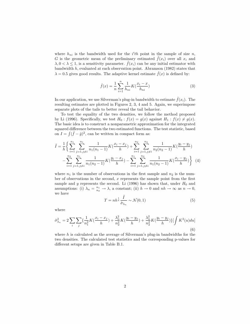
where hni is the bandwidth used for the i′th point in the sample of size n,G is the geometric mean of the preliminary estimated f(xi) over all xi andλ, 0 < λ ≤ 1, is a sensitivity parameter. f(xi) can be any initial estimator withbandwidth h, evaluated at each observation point. Abramson (1982) states thatλ = 0.5 gives good results. The adaptive kernel estimate f(x) is defined by:

f(x) =1n

n∑

i=1

1hni

K(xi − x

hni) (3)

In our application, we use Silverman’s plug-in bandwidth to estimate f(xi). Theresulting estimates are plotted in Figures 2, 3, 4 and 5. Again, we superimposeseparate plots of the tails to better reveal the tail behavior.

To test the equality of the two densities, we follow the method proposedby Li (1996). Specifically, we test H0 : f(x) = g(x) against H1 : f(x) 6= g(x).The basic idea is to construct a nonparametric approximation for the integratedsquared difference between the two estimated functions. The test statistic, basedon I =

∫(f − g)2, can be written in compact form as:

I =1h

{ n1∑

i=1

n1∑

j=1,j 6=i

1n1(n1 − 1)

K(xi − xj

h) +

n2∑

i=1

n2∑

j=1,j 6=i

1n2(n2 − 1)

K(yi − yj

h)

−n2∑

i=1

n1∑

j=1,j 6=i

1n1(n2 − 1)

K(yi − xj

h) −

n1∑

i=1

n2∑

j=1,j 6=i

1n1(n2 − 1)

K(xi − yj

h)}

(4)

where n1 is the number of observations in the first sample and n2 is the num-ber of observations in the second, x represents the sample point from the firstsample and y represents the second. Li (1996) has shown that, under H0 andassumptions: (i) λn = n1

n2→ λ, a constant; (ii) h → 0 and nh → ∞ as n → 0,

we have

T = nh12

I

σλn

∼ N (0, 1) (5)

where

σ2λn

= 2∑

i

∑

j

{ 1n2

1

K(xi − xj

h) +

λ2n

n22

K(yi − yj

h) +

λ2n

n22

K(yi − yj

h)}[

∫K2(u)du]

(6)where h is calculated as the average of Silverman’s plug-in bandwidths for thetwo densities. The calculated test statistics and the corresponding p-values fordifferent setups are given in Table B.1.

2

TABLE B.1: TEST RESULTS FOR THE DIFFERENCE BETWEEN DENSITIES

ECA dataZ-statistic p-value

Bipolar I vs. Non-bipolar I 3.008 0.0013Bipolar II vs. Non-bipolar II -0.29 0.386Bipolar I vs. Bipolar II 1.155 0.124

MHS dataBipolar vs. Non-bipolar 0.202 0.42

3