Brain Freeze: Outdoor Cold and Indoor Cognitive

Performance∗

Nikolai Cook

University of Ottawa

Anthony Heyes

University of Ottawa

University of Sussex

Abstract

We present first evidence that outdoor cold temperatures negatively impact indoor

cognitive performance. We use a within-subject design and a large-scale dataset of

adults in an incentivized setting. The performance decrement is large despite the

subjects working in a fully climate-controlled environment. Using secondary data,

we find evidence of partial adaptation at the organizational, individual and biological

levels. The results are interpreted in the context of climate models that predict an

increase in the frequency of very cold days in some locations (e.g. Chicago) and a

decrease in others (e.g. Beijing) over the next fifty years. Keywords: Climate change

- cold temperature - cognitive productivity - adaptation - climate-resilience

1 Introduction

How is the cognitive performance (“mental productivity”) of people working indoors, in

climate-protected environments, impacted by outdoor cold? To what extent can adapta-

tion at the organizational, personal, or biological level insulate against any decrement in

performance?

This paper provides what we believe to be first evidence that outdoor cold has a detri-

mental impact on performance, and to speak in detail to issues of adaptation. Data comes

from a large sample of subjects in a fully-incentivized setting.

∗Cook can be reached at ncook@uottawa.ca. Heyes can be reached at aheyes@uottawa.ca. Heyes isCanada Research Chair (CRC) in Environmental Economics at University of Ottawa and acknowledgesfunding from the CRC programme in support of this research. We are grateful to Sandeep Kapur, SoodehSaberian, Abel Brodeur, Ian Mackenzie, Lata Gangadharan and participants at Monash University, LEEPand EAERE for helpful conversations. Errors are ours.

1

Understanding the link from exterior temperature to indoor work is a key step in any

projection of how changing climate might impact productivity in sectors that are not as

obviously climate-exposed as, for example, agriculture and tourism. While the attention of

climate research in economics has been on increasing average temperatures and the effects

of hot days on human outcomes, there is a dearth of evidence of any impacts of cold. This

is an important gap in knowledge because climate models predict changes in the frequency

of cold weather.1 Even as average temperatures increase, some places will experience more

very cold days by the end of this century (e.g. Chicago), while other places will experience

less (e.g. Beijing).2 The effect of cold on the human body and behavior is distinct from that

of heat and works through different channels. Furthermore, there exists evidence that the

mechanisms for adaptation are different.

The outcome data that we use for performance is 638,238 exams taken by 66,715 adult

students over a 9 year period at the University of Ottawa, a large, comprehensive, research-

intensive public university. It operates from a main campus located in the heart of the

capital city. While the extent to which impacts on exam performance would also be seen

in workplace productivity is an open question, academic scoring reflects a clean measure of

mental proficiency which, at a minimum, seems likely to correlate with performance in a

range of brain-intensive work tasks. At least three features of our setting make it an ideal

context to explore our research question:

(1) It provides good quality cognitive performance data on a large number of working

age adults in an incentivized setting under cold and very cold exterior conditions (average

daily temperature in our sample ranges from -17◦C at the 5th percentile to 5◦C at the

95th). The data’s panel structure means we observe the same subject’s performance under

alternative outdoor-temperature treatments (on average around ten per subject), allowing

inference based on within-subject variation. This expels any time invariant within month

unobserved characteristics of individuals that might influence performance.

(2) The nature and scheduling of the cognitive tasks faced by subjects are determined

far in advance and are insensitive to subsequent temperature realizations. This allows us to

rule out selection effects due to displacement-in-time of activity in response to conditions

that could contaminate inference in other settings.

(3) While outdoor temperatures vary widely, we are able to provide direct evidence that

1 Historically Chicago (with a mean December temperature of - 3◦C) has averaged 11 days in Decemberwhere temperature remained below freezing for the whole day and a further 16 in a typical January. Thenumber of cold days in that and other mid-latitude North American cities such as Detroit and Toronto,is projected to increase between now and end of century due to increasing instability in the polar vortex(Cohen et al., 2018). Beijing has a winter temperature profile similar to that of Chicago and is projected toget less cold days.

2For a map of the effects of the polar polar vortex weakening, see Figure 6 of Kretschmer et al. (2018).

2

the indoor temperature for subjects are held almost exactly constant by modern climate-

control technology. As such, the most obvious technological protection against extreme

temperature is fully-exploited, and any effects we identify account for that margin of adjust-

ment.

Secondary data allows us to investigate non-organizational adaptation. While an em-

ployer, for example, can heat the workplace, there are actions that individuals can take to

protect against outdoor temperature conditions. We test whether reducing direct exposure

through living close to place of work provides mitigation. To investigate the hypothesis that

personal protection against extreme cold can be purchased (buying better winter clothing,

using taxis on cold days, etc.) we investigate how temperature sensitivity relates to a proxy

for subject income. To probe biological adaptation to cold conditions we (a) compare the

sensitivity to treatment of domestic students with those from overseas (in particular from a

set of hot countries) and, (b) examine how the sensitivity of the latter group evolves with

repeated exposure.

We find a negative impact of outdoor temperature on indoor performance. The effect is

substantial. In our preferred specification, which includes student fixed effects, year fixed

effects, and controls for other weather conditions, a ten degree (1.75 standard deviations)

Celsius colder outdoor temperature on exam day causes a reduction of about one-twelfth

(8.09%) of a standard deviation in performance. The magnitude and significance of the effects

prove highly robust to a wide range of tests. We speak to issues of mechanisms indirectly

by characterizing the (less-than-complete) efficacy of adaptive strategies at various levels.

While our study relates to adults taking university-level exams, such performance effects

might be expected in a wider range of mentally-demanding tasks in the workplace.

The rest of the paper is organized as follows. In Section 2, we review some pertinent

existing research. In Section 3, we detail our administrative and weather data. Section 4

presents our identification strategy. Section 5 details our main results. Section 6 explores

cumulative effects of cold. Section 7 details results on adaptation. In Section 8, we challenge

the robustness of our results. Section 9 concludes.

2 Literature: A selective review

Temperature is increasingly recognized as an important factor in many outcomes of interest to

economists. The effect of temperature realizations on productivity have been characterized

at the economy level by Dell et al. (2012), United States county level by Deryugina and

Hsiang (2014) and plant-level by Zhang et al. (2018). Recent papers have found effects

of hot weather on human outcomes including morbidity (Bleakley, 2010; Schwartz et al.,

3

2004), mortality (Barreca et al., 2016; Burgess et al., 2017), productivity (Somanathan et al.,

2015) and decision-making (Heyes and Saberian, 2019). In such studies, the temperature

observations have typically fallen in the range above 25◦C, implying little or no power to

uncover impacts of low temperatures.3

2.1 Temperature (especially cold) and mental function

Among research linking outdoor temperature to cognitive performance, such as Graff Zivin

et al. (2018), find that short-run changes in temperature negatively impact the cognitive

performance of children above 26◦C but find little evidence of longer-run effects.4 Park

(2016) studies children taking standardized exams in a panel of New York City schools

during the month of June. He finds that performance is compromised by 0.22% per 1◦F

(0.55◦C) rise above 72 F (22.2◦C). Goodman et al. (2018) focus on longer run effects of hot

weather across the school-year, finding that each 1◦F increase in school year temperature

reduces the amount learned that year in U.S. schools by about 1%.

Zivin et al. (2018) use data from the fixed date of the National Chinese Entrance Exam

to estimate the effects of outdoor temperature on cognitive performance. They find that,

in a setting without air conditioning or the ability of students to sort by location, a 1◦C

increase in summer temperatures (mean of 23.2◦C) reduced performance by 0.029 standard

deviations.

Research on the effects of cold temperature on mental performance and productivity is

less developed. With one notable exception, the evidence that does exist relates exclusively

to contemporaneous temperature. In other words performance and behavior during exposure.

Pilcher et al. (2002) provides a meta-analysis and Taylor et al. (2016) a survey.

Without identifying a mechanism, various experimental studies have shown that contem-

poraneous exposure in the range - 20◦C to 10◦C can reduce memory function (Thomas et al.,

1989; Patil et al., 1995), consistency of decision making (Watkins et al., 2014), and speed in

pattern recognition and number comparison (Banderet et al., 1986). Studying driving be-

havior in cold conditions, Daanen et al. (2003) note that cold can impair mental function and

3Lee et al. (2014) regress outdoor temperature on speed of completion of a routine clerical task by bankemployees in Tokyo. They find a negative and significant coefficient on their quadratic temperature term,consistent with a positive impact of either extreme heat or extreme cold on productivity. However; (1) Themean and standard deviation of outdoor temperature in the table of summary statistics are 17◦C and 5◦Crespectively, suggesting few observations in the temperature range of interest to us. (2) The authors do notallow for the possibility of asymmetric impacts of heat versus cold by (for example) applying non-parametricmethods.

4They explicitly acknowledge that they can speak to high temperatures only: “Since these tests werepredominantly given during the warmer periods of the year, our analysis of short-run temperature effectswill only be informative for temperatures in this range” (Graff Zivin et al., 2018, p.84). In their dataset, forexample, the mean temperature on day of test is 22.5◦C and standard deviation 4.9.

4

thus increase accidents, observing a 16% decrement in performance of drivers in simulated

conditions at 5◦C compared to 20◦C.

There are several channels that might link cold to compromised cognitive performance.

In their survey, Cheung et al. (2016) emphasizes the depleting effect of thermoregulation.

The initial response to short-term cold exposure is cutaneous vasoconstriction, reducing

blood flow to the skin and extremities. This serves to decrease the thermal gradient between

the body and environment. While this is effective in maintaining body core temperature,

it simultaneously causes discomfort. As exposure persists, heat maintenance requires the

depletion of limited carbohydrate stores (Bell et al., 1992) which has been shown to decrease

manual dexterity, motor coordination, work tolerance, and “perceptual discomfort that can

effect cognition” (Cheung et al., 2016, p.155). Exposure to cold conditions also alters the

concentration of central catecholamines in humans which has been linked to “... a detri-

mental effect on cognition as brain regions such as the prefrontal cortex are reliant on these

neurotransmitters for normal function, ... (as such) there is a plethora of evidence which

demonstrates that tyrosine supplementation improves cognitive function during acute cold

stress” (Taylor et al., 2016, p.372). Breathing very cold air can also irritate the human

respiratory system, potentially damaging mood (Hartung et al., 1980), while even brief cold

exposure can elevate hormonal stress markers (LaVoy et al., 2011).

A parallel body of research highlights the role of psychological mechanisms. Consistent

with the classic “distraction theory” of Teichner (1958), cold conditions may provide alter-

native stimuli and thus interrupt focus which would otherwise be applied to the cognitive

task in hand (“i.e., attention is focused on feeling cold rather than competing the cognitive

task provided” (Taylor et al., 2016, p.372). Uncomfortable temperatures might also influence

motivation and performance via their negative effect on mood or sentiment (see citations in

Noelke et al. (2016)). The case for the importance of psychology is reinforced by studies such

as Rai et al. (2017), which show that the attitudes and behaviors of experimental subjects

can even be influenced by temperature cues, such as photographs of cold places.

While such studies are suggestive, they offer little help in understanding what the wider

impact of cold outdoor temperature might be across the economy, since the vast majority

of mentally-taxing work in cold countries is done indoors. Indeed, in most industrialized

countries the median adult spends more than 90% of their time indoors, particularly during

cold weather (Nguyen et al., 2014). Nguyen et al. (2019) finds similar effects for children, as

when especially cold weather occurs more time is spent inside.

To our knowledge, the only study examining the sustained impairment due to cold expo-

sure after stimuli is removed is Muller et al. (2012). They track a sample of 10 young adults

during and after being cooled in a temperature-controlled chamber at 10◦C. Working mem-

5

ory, choice reaction time and executive function declined during exposure, and impairments

sustained an hour after exposure. This points to the possibility of the impact of exposure to

outdoor cold being something that the subject imports when they move indoors. Relatedly,

Heyes and Saberian (2019) argue that uncomfortable outdoor temperature might affect in-

door performance even if the subject is not directly exposed to it. For example, extreme cold

may prevent or discourage subjects from going outside to ‘stretch their legs’. Lack of fresh

air has been linked experimentally to outcomes such as decreased mental function (Chen

and Schwartz, 2009) and depressive mood (Cunningham, 1979).

2.2 Adaptation

Adaptation to cold outdoor temperatures might occur at various levels (for example national,

municipal, organizational, individual) and over time. In this paper, we present short-run

analyses that will net out avoidance measures that are based on historical climate, such as

locational sorting, technology adoption and building design.

The first and most obvious short-run protection against cold weather is to move indoors.

The extent of protection afforded by a building plausibly depends on the effectiveness of its

interior heating. At the other end of the temperature spectrum, the analogous protective

benefits of air conditioning have been explored in a number of studies. Park (2016) study

New York City children taking Summer exams, and does not find a significant protective

benefit to air conditioning. He does note that of schools with air conditioning installed, up

to 40% were deemed defective by an independent survey. In contrast, Goodman et al. (2018)

finds that school level air conditioning offsets most of the potential learning decrement due

to heat.5

A related literature studies the mitigative effects of other ‘technologies’, such as invest-

ment in high quality winter clothing (Makinen, 2007). We will explore pecuniary channels

of self-protection later.

Biological adaptation may also be physiological or psychological, though evidence on

each is comparatively scarce. Teichner (1958) developed the concept of psychological cold

tolerance “... which was conceived as depending largely on the individual’s familiarity with

cold and on his anxiety level. These are factors reflected in the individual’s subjective

reactions which should not be ignored when discussing performance in the cold.” (Enander,

1984, p.370). In terms of such habituation there is some evidence of changes in attitude

5 Goodman et al. (2018) uses a triple-difference strategy combining within-student observations withwithin-school variation status in cooling status over time. The only threat to such an approach is thepossibility that the timing of A/C installation was correlated with other unobserved improvements in learningenvironment.

6

to cold after repeated exposure. In early work, Fine (1961) showed that subjects evaluate

‘cold’ less on a cold-warm scale after repeated exposure. Enander et al. (1980) compared the

response to cold of subjects accustomed to working in cold conditions (meat cutters) against

office workers. While there was no difference in physiological response, they found evidence

consistent with psychological adaptation. The accustomed group experienced significantly

less cold sensation and pain than the unaccustomed group. Another study consistent with

physiological adaptation is Tochihara (2005), who found that the rectal temperatures of a

sample of coldstore workers fell less when exposed to a temperature of -20◦C for 60 minutes

than did those of the control sample.6 Several studies have found evidence consistent with

increased brown adipose tissue (‘brown fat’) among those exposed to frequent cold (for

example Blondin et al. (2014)).

Overall, the bulk of the evidence points to a primarily psychological adaptive process

to cold. This provides an interesting contrast to the analogous evidence on adaptation to

heat exposure. “(T)he evidence of physiological adaptations from longitudinal cold exposure

is equivocal (Launay and Savourey, 2009), while the dominant adaptation is a perceptual

habituation and desensitization to cold stress rather than large-scale systemic physiological

changes of the sort seen with heat acclimatization” (Cheung et al., 2016, p.155).7

2.3 Projected change in cold

It is commonly assumed that as climate warms, the distribution of daily temperatures will see

a rightward shift towards warmer averages. In isolation, this would indicate that problems

of extreme cold temperatures may be alleviated due to warming temperatures. However,

while this turn out to be the case in many places - in which case the effects that we uncover

in the paper will deliver a previously unaccounted for benefit of climate change - in others

it will not.

Hansen et al. (2012) showed that the chances of unusually cool seasons have risen in the

past 30 years, coinciding with the observed rapid global warming. One mechanism through

which this has been studied is a weakening of the polar vortex, which makes easier the

6Brazaitis et al. (2014) immersed 10 male subjects in 14◦C water and timed how long it took for bodytemperature to drop to 35◦C. On day 1 the average cooling time was 130 minutes, on day 14 cooling timehad fallen to 80 minutes. The authors suggest a reduction of temperature gradient as a possible adaptationto cold.

7 The abstract in the survey of physiological adaptation by Daanen and Van Marken Lichtenbelt (2016)ends: “Dedicated studies show that repeated whole body exposure of individual volunteers, mainly Cau-casians, to severe cold results in reduced sensation but no major physiological changes. ... (H)uman coldadaptation in the form of increased metabolism and insulation seems to have occurred during recent evo-lution in populations, but cannot be developed during a lifetime in cold conditions. Therefore we mainlydepend on our behavioral skills to live in and survive the cold” (Daanen and Van Marken Lichtenbelt, 2016,p.104).

7

periodic southerly movement of cold Arctic air masses. Kolstad et al. (2010) and Kretschmer

et al. (2018) show that in the past several decades the frequency of weak polar vortex states

has increased, which has been accompanied by subsequent cold extremes in the mid-latitudes,

including North America, Europe and northern Asia. Kim et al. (2014) find evidence linking

weakening of the vortex to Arctic sea-ice loss, consistent with the trends associated with

climate change. “A handful of studies offer compelling evidence that the stratospheric polar

vortex is changing, and that this can explain bouts of unusually cold winter weather (in

North America)” (Francis, 2019).

3 Data

We obtained administrative data from the university as the basis for our measure cognitive

performance. In particular, we observe the universe of grades achieved by undergraduate

students for over 1.2 million courses. Our sample includes students who first enrolled for

a course at the university in or after the Fall semester of 2007, and the latest courses we

observe are those examined in December 2015. We connect this dataset with institutionally

provided student information such as gender, age and address. Data on financial status by

six-digit postal code comes from the 2016 Canadian Census of Population.

The academic year is split into two semesters. Fall-semester courses are taught from

September through November, with final exams written in December. Because of our interest

in cold we use these grades (N = 638,238) and the students that achieved them (N = 66,715)

as the basis for our analysis.

That course-level grade is our dependent variable introduces a complication. While we

hypothesize that exam day temperature impacts performance in the final exam, assessment

for each course is based only partially on final exam performance. Other elements such as

midterms or coursework completed during the semester also contribute. Academic regula-

tions require that final exam weight be no lower than 40% and no higher than 60%. The

variation in weighting adds measurement error to the dependent variable which is uncor-

related with our regressor of interest.8 While such measurement error does not bias OLS

estimates, it increases the associated standard errors making significance claims conserva-

tive. It also requires that in interpreting effect sizes, we use a multiplier to reflect that any

impact of exam-day temperature on exam performance has a dampened impact on course-

level performance. In our main specifications we impute the variation in exam performance

8The granularity of course grade reporting is an additional source of measurement error. Final coursegrades are recorded as letters, which correspond to a score interval. For example, an ‘A’ corresponds to ascore in the interval 85-89%, which we then assign to the midpoint of its interval.

8

as a factor of two times the variation in course performance, consistent with the assumption

that the final exam carried 50% of the weight in every course. In doing so, a 5% decrement

in overall course score maps to a 10% decrement in final exam score.

Daily meteorological data comes from the nearest Environment Canada weather station

that provided consistent data across out period (Station ID 6105978) located 5.1 km from

the centre of the campus. There is wide variation in the outdoor temperatures experienced

by students on exam days, illustrated in Figure 1.

Summary statistics relating to course performance, student characteristics and weather

are in Table 1. The average course grade is 71.98%, corresponding to a ‘B’ in the university

grading scheme. Grades vary considerably within-student, the standard deviation is 10.31%,

or two letter grades around the mean. Exam days are cold, averaging -5.13◦C. Temperatures

also vary considerably within-student, as a one standard deviation colder temperature is

-10.81◦C while a one standard deviation milder temperature exam day is above freezing.

There is often snow falling (the equivalent of 2.12 cm)9 and snow already on the ground

(2.46 cm). Female students account for 60% of the data while foreign students contribute a

healthy 7.43%. We use a total of 638,238 exams, written by 66,715 students. The succeeding

columns present summary statistics by gender and foreign status.

4 Methods

In this section we detail the identification strategy used to estimate the causal impact of

outdoor exam temperatures on indoor cognitive performance (imputed exam score).

Identification comes from quasi-random assignment of exterior temperatures to exam

days. Fall semester exams are held in an exam period that runs from early in December

until the university closes for the Christmas recess. The earliest and latest dates on which

we observe exams in our sample are December 4 and December 21. Exams are held in one of

three time slots (beginning at 9:30 am, 2 pm and 7 pm).10 The university releases the exam

schedule in mid-October, much later in the semester than the final class enrolment deadline

(mid-September).

Our results use a student fixed effects model estimated by Ordinary Least Squares (see,

9Environment Canada uses a 10-to-1 conversion of water equivalent precipitation and snowfall.10We do not observe students allowed to defer an exam to a date other than that mandated for the course,

typically about 4% of the total. Deferment for reasons unrelated to temperature (family bereavement,religious holiday, etc.) are of no concern. Insofar as some deferments result from low exam-day temperatureit is plausible that it works against the direction of any effect that we find, since postponement from a daythat is unusually cold is likely to be to a later date that is less cold. However this is a valid caveat to holdin mind. Note that the university as a whole never closed on a regular business day or canceled an exam forweather-related reasons during the study period.

9

for example, Ebenstein et al. (2016)). Our main specification is:

Gradei,t = β0 + β1 ∗ Temperaturet + ∆t + γi + ηy + εi,t (1)

Where Gradei,t is the imputed exam performance for individual i taking a course where

the final exam took place on day t. Our parameter of interest is β1, the coefficient of mean

outdoor temperature on the date of exam. We explore the robustness of our estimate using

alternative temperature measures later. The standard errors are clustered at the student

level. Later, we demonstrate the results’ robustness to alternative clustering.

The inclusion of student (γi) and year (ηy) fixed effects implies that identification comes

from within-student and within-year variation. In other words, variations in the performance

of individual subjects under alternative temperature treatments, within an exam period.

Year fixed effects capture changes to course grades between years that are common across

students including, for example, grade inflation.

∆ is a vector of exam-day controls – precipitation on exam day and its interaction with

temperature, relative humidity, snow on ground, windchill, day of week indicator variables

and the date-in-month.

Inclusion of the interaction term between temperature and precipitation in our specifi-

cations reflects the common observation that damp cold may have a different effect than

dry cold. For the same reason relative humidity is included as an additional control in our

preferred specification. The interpretation of β1 is the effect of a 1◦C change in exam tem-

perature on a dry day. There is zero precipitation on 45% of the days in our sample, and

less than one millimeter of precipitation on 62% (see Figure A2 for a full distribution). A

robustness exercise shows that effect sizes sustain even when we estimate on dry days alone.

We also present estimates without precipitation, or its interaction, in an appendix.

Precipitation in December almost always means snow at this location. In addition to

precipitation actually falling on a particular day, we also include accumulated snow on ground

(measured by Environment Canada’s acoustic sensors such as the SR-50A). Accumulated

snow might effect ease of travel, although it is worth noting that the municipal government

exerts considerable efforts to the clearance of snow from sidewalks and streets in the city, as

does the university on its campus. Actual experience of snow under-foot in the vicinity of

a downtown location such as the university campus is likely quite different to conditions at

the weather station.

Day-of-week and date-in-month controls capture the possible effects of exam timing.

Although temperature should be uncorrelated with day of week, a simple regression with

temperature reveals that exams written on Sundays are significantly colder than the rest of

the week. For this reason we include day-of-week controls. Date-in-month (as a continuous

10

variable) captures any variation in exam performance correlating to when in the month the

exam takes place. For example, including date-in-month helps if “difficult” courses tend to

have exams scheduled later in the month, or if proximity to the holidays has an effect on

exam performance.

In a supplementary analysis we explore the possibility of a non-linear relationship between

outdoor temperature and indoor performance. To do this we estimate two models. First, our

continuous temperature regressor in Equation 1 is replaced by a series of indicator variables

corresponding to bins of width 2.5◦C. Second, we use a series of indicator variables that

organize temperature treatments into deciles.

5 Results

5.1 Basic plot

Figure 2 provides a simple plot of exam day temperature and exam performance, after

adjusting only for year of exam. The size of markers is proportional to the number of

observations in each 0.5◦C bin.

Visual inspection suggests a positive association between performance and exam day

temperature. We formalize this by plotting the line of best fit estimated by OLS with only

year fixed effects.

While the absence of plausibly important controls means that such a plot and associ-

ated fitted line should be treated with caution, these initial effect sizes are substantial and

prove robust to the inclusion of controls and their associated alteration of the temperature

coefficient’s interpretation.

5.2 Linear

Our main results are reported in Table 2. The dependent variable is expressed in hundredths

of a standard deviation of exam score. Standardization of grades is across all years and

students.11

Column 1 presents our sparsest specification, containing student and year fixed effects

and accounts for precipitation and the precipitation × temperature interaction.12 Column

11In Table A4 we standardize by year and course to find similar, if not larger, estimates.12In Table A1 we also report our analysis without precipitation or its interaction with temperature. We

then report the coefficient of precipitation and its interaction with temperature, and find both are negativeand statistically significant. A specification in which we drop all controls is reported as a robustness exercisein Table 12, and delivers a main coefficient of 1.526***.

11

2 adds controls for day-of-week. Column 3 controls for date-in-month. Column 4 through 6

add relative humidity, accumulated snow on ground and windchill, respectively.

In each column, the estimated coefficient on temperature is positive and statistically

significant beyond the 1% threshold. Coefficient values are also stable across specifications.

Column 6 presents our preferred specification, corresponding to Equation 1.

The coefficient on temperature is 0.809***, suggesting that for every 1◦C increase in exam

day temperature, performance increases by 0.00809 standard deviations.13 The 90th and 10th

percentiles of the temperature distribution in the sample are 2.2◦C and -14.7◦C respectively.

Hypothetically moving from a day at the 90th percentile in terms of temperature, to a day at

the 10th percentile, delivers a decrease in temperature of 16.9◦C. According to our preferred

estimate this causes a substantial decrement in exam performance of 0.14 about one-seventh

of a standard deviation. Equivalently, to deliver a reduction in performance of 0.1 or one-

tenth of a standard deviation would require a 12.4◦C decrease in outdoor temperature.

5.3 Non-linear

In Table 3 we repeat the exercise just described but replace the continuous measure of

exam day temperature on the right-hand side of Equation 1 with a series of eight indicator

variables. Each takes the value 1 if average temperature on exam day t fell in the range

that defines the associated indicator’s bin. Bins are constructed to be 2.5◦C in width, built

out from zero. The bin containing days with temperature below -17.5◦C is the reference

(omitted) category.

Each column in Table 3 replicates the combination of controls in the same-numbered

column in Table 2. The preferred specification is again reported in column 6. The coefficients

for each bin are broadly consistent across columns, suggesting that estimated non-linear

effects are also robust to the inclusion of alternative control sets. The coefficients and

associated 5% confidence intervals from the sparsest (column 1, left panel) and preferred

specification (column 6, right panel) are plotted in Figure 3.

Figure 3 shows a negative impact of cold outdoor temperature on performance, which

is roughly linear over the range that we study. The vertical axis scale in both figures is

hundredths of a standard deviation. For example, in the right-hand panel of Figure 3,

moving from a day in the 0◦C bin to the -15◦C bin reduces course grade by about 12% of a

standard deviation.

13 It is possible that exam markers adjust their grading standards in response to the quality of responsesin a particular pile of scripts. Insofar as that is the case it seems likely that the correlation between gradingstringency and response quality is positive (the marker would apply laxer standards if she found the studentsperforming poorly). This would imply that our estimated coefficient would understate the true effect size,making inference conservative.

12

In Table A2 and Figure A1, we use temperature deciles to conduct a similar analysis.

We find results consistent with using the 2.5◦C temperature bins.

5.4 Heterogeneity

In this subsection we investigate heterogeneity of effect size by sex, ability, and foreign status

of the student. To do this we add to the preferred specification, in separate exercises, inter-

action terms between temperature and an indicator variable for the subsample in question.

The results of these exercises are reported in Table 4.

In column 1 we interact temperature with an indicator that takes value 1 if the student

is female. The estimated coefficient of 0.927*** is for a male student. The negative and

significant interaction term implies that ceteris paribus female students are about twenty

percent less sensitive to cold, consistent with research that has found women wear both

more layers and more articles of clothing in cold weather, regardless of activity (Donaldson

et al., 2001).

In column 2 we conduct the same exercise but with an indicator that takes value 1 if a

student arrived at the university with an A (or 80) admission average. This applies to 43%

of our sample of exams. The coefficient on the interaction term is large in value, -0.311***.

The central estimate suggests that these high-admission students are roughly one third less

cold-sensitive than their counterparts.

In column 3 we conduct the same exercise on foreign students, using domestic students

as a baseline. Classification as foreign student is derived from paying international student

fees to attend the university, or through immigration status. Perhaps unsurprisingly, foreign

students are around 60% more sensitive to cold than domestic students. Almost all foreign

students come from countries that are substantially less cold than Canada, and so are unlikely

to be accustomed with such temperatures. We provide evidence of habituation or biological

adaptation by investigating the performance of foreign students, both on arrival and through

time, later.

6 Cumulative effects

While not our main focus, before turning to adaptation we investigate effects of temperature

not just on the exam day, but during the preceding teaching semester.14

14 Evidence of the cumulative effect of temperatures on cognitive performance is mixed. For example, withrespect to much warmer temperatures Goodman et al. (2018) found no cumulative effect of temperature onlearning in United States schools with A/C.

13

To do this we add to our preferred specification, a proxy of the total ‘cold’ experienced

in the 30, 60 and 90 days prior to the exam. The measure that we use for cumulative cold

is total heating degree days (HDD) over the period in question. A HDD is the number of

degrees that the average temperature on a particular day is below 18◦C, and is the standard

measure used to quantify cumulative demand for heating in buildings. For example, if in a

30 day window half the days have an average temperature of 12◦C while the other half have

an average temperature of 17◦C, the total HDD count over that 30 day window would be

(15 x 6) + (15 x 1) = 105.

Table 5 reports the results of these three exercises. Columns 2, 3 and 4 include the total

HDDs in the 30, 60 and 90 days prior to first exam, respectively.15

The results in this table are interesting for two reasons.

First, as a robustness check on our main result. The coefficient on our primary indepen-

dent variable of interest, same-day temperature, is stable across columns. This suggests that

we have isolated short from longer-run temperature effects. A potential challenge to our

main specification is that temperature on exam day may be correlated with how warm or

cold it had been in the lead up to the exam, such that failing to control for the latter would

bias (or completely explain) our central estimates. Comparison of the columns in this table

discourages the view that any such bias has substantially distorted our results. To ensure

that this is not an artifact of the HDD measure, we report the results of analogous exercises

using either average temperatures or much shorter pre-exam windows in Appendix Tables 2

and 3. We find our coefficient of interest is little-disturbed.

Second, in each of columns 2 through 4 the estimated coefficient on the pre-exam his-

tory of HDD is statistically significant. Temperature during the semester appears to have

a significant impact on how students perform. However the sign is positive, implying cooler

temperatures across the teaching term are associated with improved performance. This is

consistent with previous literature that finds unappealing outdoor temperatures can encour-

age substitution from outdoor leisure to indoor ‘work’ (Graff Zivin and Neidell, 2014). For

example, in column 2, if each day in the 30 leading up to the exam were one degree warmer,

that would roughly offset exam-day temperature being one degree colder.

Another consideration could be cold temperatures leading to student sickness. While

we do not have case-level data of, for example, admissions to the university clinic, we do

analyze how short run temperatures leading up to the exam affect performance in Table A3.

We find previous 1,3, and 5 day average temperatures leading to the exam have mixed signs

and statistical significance. We note that this measure is imperfect and see examining the

relationship between cold and sickness as a possible avenue for future research.

15In Table A3 we use average temperatures leading to exam day, the results are similar.

14

7 Adaptation

Central to any analysis of the costs of climate change is understanding the efficacy of adap-

tation. Analyzing adaptation also speaks indirectly to mechanisms that might underpin the

effect that we have identified. We explore adaptation at three different levels.

7.1 Organizational

There are two temperatures that might influence how a worker performs, namely indoor and

outdoor. The employer can control the former, but not the latter.

There are two separate questions that research in this area can address. First, to what

extent is the technology of climate control effective in decoupling indoor from outdoor tem-

perature. Second, insofar as is it does lead to full or partial decoupling, to what extent does

that mitigate the causal effect of outdoor temperature on the outcome variable of interest.

With respect to hot temperatures, recent studies provide evidence of only partial mitiga-

tion by air-conditioning. These share two important limitations. (1) Installation and quality

of air-conditioning is unlikely to be randomly-assigned, and in many settings is plausibly

correlated with unobserved characteristics (such as financial circumstances) of the school,

business or other organization that might impact effect size through other channels. (2) To

our knowledge, the actual efficacy of the cooling technology is unknown.16

Winter heating in Ottawa public buildings is good, perhaps not surprising given that very

cold temperatures are common. Employers in Ontario (including universities) are obliged by

law to maintain a workplace temperature above 18◦C. In light of this, internal temperatures

experienced by our subjects are plausibly uncorrelated with outdoor temperature by design.

However we tested this directly by working with campus building managers to measure and

collect data on daytime interior temperature. The sample was collected during December

2018 for the 28 most important exam rooms by contribution to sample. Matching with

outdoor temperature on the same day, we investigate the links between indoor versus outdoor

temperature in exam rooms.

16Quinn et al. (2014) and Tamerius et al. (2013) present survey evidence on the relationship between indoorand outdoor temperatures in a sample of 327 buildings in New York City. For outdoor temperature rangesabove 15◦C they find a correlation between outdoor and indoor temperature to be 0.64 (Tamerius et al.,2013, Fig.1) despite air-conditioning penetration in that city at time of sample being 87.5%. Interestinggiven our focus is that for temperatures below 15◦C the correlation coefficient between indoor and outdoortemperature is just 0.04. In general, heating space is easier than cooling it. In addition, modern air-conditioners are characterized by a ‘temperature drop’ - the maximum by which the refrigerant coils canreduce incoming to outgoing temperature - which for most common designs is less than 20◦C. Even if workingto its full potential, this places a bound on how cool the air-conditioned space can be kept when outdoortemperatures are very high.

15

The data collected for Montpetit Hall Room 021 (MNT021) is presented in Figure 4. This

is the largest room by contribution to sample, contributing 66,888 of the 638,238 observations

that we use in our regressions. There are two important features of this plot. First, there

is little variation in indoor temperature, fluctuating between 21.5 ±0.3◦C (reference lines at

±1◦C of the room average are provided). Second, such variation as does exist does not look

to be meaningfully correlated with outdoor temperature.

Figure 5 presents analogous diagrams for each of the 28 rooms (MNT021 is third from

the left, second row). In each case we superimpose horizontal reference lines at the room’s

average temperature ±1◦C. The figure tells us that all exam rooms are not equal in terms

of the consistency with which internal temperature is maintained. In some rooms internal

temperature fluctuates outside the ±1◦C corridor, though even in these ‘leaky rooms’ there

is little suggestion of correlation between outdoor temperature and what is going on outside.

We conduct two further exercises to test whether our central results are driven by im-

perfect climate control.

First, we test the role of building age. Our sample includes both new and old buildings.

For example, Tabaret Hall (TBT) was constructed in 1856. While spaces are well maintained,

there is a concern that our results are driven by older buildings that do not meet modern

standards. To explore this we divide buildings into two categories, ‘New’ (those completed

after the year 2000), and ‘Old’ (the rest). This roughly splits our sample in half. Column 1 of

Table 6 reports the results of adding to our main regression an interaction term that between

exam-day temperature and an indicator variable that takes the value 1 if the exam room

is located in a new building. The interaction term is negative, and marginally significant,

consistent with our concerns. The estimated coefficient on temperature (0.837***) is now

interpreted as the effect of temperature on performance for exams written in an old space.

Writing in a new building is estimated to offset about 14% of the outdoor temperature

effect.17

Second, we exploit the room temperature measurements reported in Figure 5 directly.

Even within a building some rooms may be better temperature-controlled than others. In

column 3 of Table 6 we report the results from running the specification from column 2 but

excluding the exams taken in rooms identified as ‘leaky’ in Figure 5 (that is, those with

temperature observations outside the ± 1◦C band). Under this restriction the coefficient

of the new building × temperature interaction term becomes much smaller and far from

statistically significant at conventional levels.

17For completeness we repeat the specification in column 1 but including course level fixed effects, as theremay be a relationship between building age and course level. This is reported in column 2 in Table 6. Theadditional inclusion does not change results, and increases the statistical significance of the new buildingand temperature interaction term.

16

Taken together, the evidence in this subsection supports our conjecture that the most

obvious technological adaptation that an organization can use to protect employees against

cold, namely climate control, is relatively fully-exploited. As such, the effects that we identify

should be understood as already accounting for that base margin of protection.

7.2 Individual

Individuals plausibly have ways in which they might protect themselves privately from cold.

We explore two. One approach is to reduce exposure by reducing commuting time. Another

is spending on personal protection.

First, we examine the extent to which our effect dissipates with proximity to campus.

We note that residential location and commuting time is not randomly assigned in our

setting. Students might reasonably be assumed to take account of climate when deciding

where within the city to live, and results in this section need to be interpreted with that in

mind. We add to the preferred specification a control for distance between campus and term

address as recorded in the student record (‘Distance’). We then linearly interact distance

with exam day temperature. For completeness, we also add the interactions between distance

and precipitation, and between distance and accumulated snow on the ground. The results

are presented in column 1 of Table 7. The estimated coefficient of temperature × distance

is 0.000 and not statistically significant, suggesting no protective effect of proximity. That

is, as a student moves closer to the university there is no reduction in the sensitivity of

their performance to outdoor temperature. Reassuringly, the coefficient on the primary

temperature regressor is not meaningfully disturbed.

An issue about the exercise just described is that we observe two distinct addresses

for each student. First, an enrolment address used during a student’s application to the

university. This is almost always the parental or home address. Second, the term address

that students are encouraged to keep updated. For some, the application address will be

where they actually live, for some it will not, and the lack of variation reflects a failure to

update personal details rather than a lack of relocation.

Ideally, we would like a sample of students for which we know where they live with some

additional assurance. We construct something close to this in two ways. First, we identify

those students who have a term address distinct from that at enrolment. We call these

students ‘movers’.18 Second, we identify those students who are non-movers but for whom

the application address is within 10 km of the university campus. These students live within

18While it is possible that some families might move in the period between receiving offer and the start ofstudies, this number is likely small.

17

ready commuting distance of the university and in most cases live at home during their

studies, something that is common amongst Canadian undergraduates.

Column 2 reports the results from movers and column 3 from non-movers with an enrol-

ment address within 10 km of campus. The main temperature coefficient of interest remains

similar across the three samples, and in each case is statistically significant, despite much

eroded sample sizes in column 2 and 3. The coefficients on the temperature × distance inter-

action are small and insignificant at conventional levels, discouraging the view that proximity

alone delivers a meaningful protective benefit.

In Table 8 we present results of a different approach. We stratify by distance the sample

of students who report a term time address within 20 km of campus, irrespective of whether

or not they are in our movers sample. In most cases the address that we use is likely

the student’s residential address. The estimated coefficient on temperature is stable across

columns, even in column which estimates only on students who are ‘currently’ living within

2 km of campus.

Subject to the caveats already noted, the exercises presented in Tables 7 and 8 provide

no indication that living close to place of work mitigates the effect of outdoor cold on perfor-

mance. To the extent that distance correlates with direct exposure to outdoor temperature

this implies that it is not the ‘amount’ of direct exposure which drives the decrement in

performance. A similar impact of cold weather is seen even among those who live close to

campus. This is more consistent with psychological rather than physiological mechanisms,

or other channels identified that do not depend primarily on exposure length.

Apart from locational choice, there may be pecuniary ways in which individuals may

mitigate the effects of weather to their person. For example, a student may invest in better

quality winter clothing, or avoid waiting for a bus by using taxis on particularly cold days.

Here we explore a possible role of affluence in temperature-protection.

We do not directly observe the financial circumstances of our sample. However we do

know the address reported at first enrolment, which is likely the parental or home address.

As a proxy for financial circumstances, we use the average income level at the associated six

digit postal code at enrolment as measured in the 2016 Canadian Census. We add this to

our preferred specification as an interaction term only, as the student fixed effect will already

have accounted for individual income. We present these results in Table 9.

In column 1 we work with all students, including foreign students, provided they had

an eligible six digit postal code at enrolment. Because there exists the possibility that the

Canadian address reported for a foreign student may a poor indicator of familial wealth,

we restrict our sample to domestic students in column 2. In either specification, the main

coefficient remains positive and significant. It is somewhat larger than in Table 2, and is

18

now interpreted as the effect on a student from an enrolment address in a hypothetical

postal code with average household income of zero dollars. The negative and significant

coefficient on the temperature × average income interaction indicates a protective effect of

family affluence. Each 10,000 CAD increase in average household income in postal code of

origin is associated with a 3.7% reduction in the sensitivity of a particular student to cold.

A histogram of household incomes is presented in Figure A5. Compared to a zero income

benchmark, a student coming from a postal code in the modal category (namely 40,000 to

50,000) benefits from a roughly 15 - 19 % mitigation of cold sensitivity.19

Overall these exercises are consistent with a protective, but still less than complete, effect

of family affluence.

7.3 Biological

In this section we present evidence consistent with the results of small scale studies of

physiological or psychological adaptation to extreme temperatures mentioned in Section 2.

We do this by looking in more detail at the cold-sensitivity of students from other countries

and how they evolve over time.

In Table 4 we established that foreign students were statistically more cold-sensitive

than domestic students. That Canada is a cold country implies that most students from

abroad are from warmer climates. Despite our data not including country of origin at the

student level for privacy purposes, we construct a subsample of students most likely to be

‘hot’ countries by leveraging their language of instruction. The University of Ottawa is the

largest bilingual English-French university in the world and many undergraduate programs

can be taken in their entirety in both languages. As part of its cultural mission the university

encourages applications by students from countries of the Francophonie through substantial

fee reductions, scholarship programs and promotional efforts.20 41% of foreign students use

French as their language of correspondence with the university. Without knowing individual-

level country of origin, the overwhelming majority of non-domestic come from the nations

of French Africa (Cote d’Ivoire, Senegal, Cameroon, etc.), or the French Caribbean (Haiti,

Dominican Republic etc.) at the aggregate level. These are all hot countries with winter

low temperatures typically 25 to 40 degrees Celsius warmer than Ottawa. We identify these

students in two ways. First, we construct a sample comprising foreign students that elect

19Caution should be used in interpreting these results, as the astute reader would note a linear modelpredicts an income of 267,838 CAD would perfectly offset, and above that reverse, the effects of cold. Whilewe do not see such wealth in our data due to measurement at the postal code (rather than individual) level,it is reasonable to assume that there are diminishing returns to wealth.

20 For example foreign students from French-speaking institutions pay domestic rather than foreign fees,which for 2014 - 15 implies a reduction from 22 600 CAD per year to 6,800 CAD.

19

to study entirely in French across all four years of their program (‘Method 1’). Second,

reflecting that many students who arrive as unilingual French will develop their English-

language skills sufficiently to take at least part of their later studies in English, we relax the

sample criterion to comprise foreign students that elect to study only French-taught courses

in their first year (‘Method 2’).

Column 1 in Table 10 reports the result of estimating our preferred specification on the

Method 1 subsample, with column 2 estimated on remaining foreign students (most of which

come from China and the United States). We can see that the effect of cold on hot country

students is much larger than even the effect on international students in general (column

2). The central estimate suggests that a 10◦C reduction in outdoor temperature causes a

decrement in performance of almost half (45.9%) of a standard deviation. The results in

columns 3 and 4 are those estimated on the subsample constructed on the basis of Method

2. They are consistent, though the implied decrement in performance for a 10◦C reduction

in outdoor temperature is somewhat smaller at 29.9% of a standard deviation.

The results presented to this point have been based on within-student variation in per-

formance under different temperature treatments across their entire period of study. Here

we explore how the performance of arrivees changes over time.21

The results in Table 11 are estimated only on exams taken during the first year of

enrollment. Because this specification incorporates a temperature × foreign interaction term,

the estimated coefficient on temperature, 1.124** represents the effect of temperature on a

domestic students, within a course level, during their first exam season. That the coefficient

on the temperature × foreign interaction regressor is positive and significant confirms the

earlier finding that foreign students are much more cold-sensitive in their first year.

This exercise is important for another reason. If cold winter temperatures directly affect

student attrition rates, then in all specifications we are estimating on temperature ‘survivors’.

Our results could then be attenuated, particularly at upper course levels. By estimating

column 1, we better approximate the effect of cold on performance absent students self-

selecting out during the course.

Column 1 is estimated on all students, irrespective of whether they graduate. In column

2 we conduct the same exercise, looking at courses taken in first year of enrollment, but

now only by those students that ultimately graduate. This is more akin to a balanced panel

estimate than the earlier results, and addresses any concern that the propensity to select

out of sample during the course of a program might be different between domestic and

21 All specifications include a course-level fixed effect (e.g. second-year or 2000-level courses), to disentanglethe effect of course difficulty from the number of years enrolled. The correlation between course level andyears enrolled is 0.65.

20

foreign students. The results here suggest that among domestic students there is indeed

disproportionate attrition of cold-sensitive students, as we would expect, but little evidence

that the same applies to their foreign counterparts.

To explore adaptation over time, in column 3 we look at all exams taken, but include an

interaction term between temperature and number of years enrolled. The exercise is repeated

in column 4 where we restrict attention to that subset of students who ultimately gradu-

ate. The temperature × years enrolled coefficients are small and statistically insignificant,

indicating that as domestic students spend more time at the university their sensitivity to

cold does not change. The large and statistically significant coefficient on the triple interac-

tion term – how foreign student’s sensitivity changes over time – indicates as these students

spend more time in Ottawa they become substantially less sensitive to cold. Among both the

entire sample and the students who ultimately graduate, the differential between domestic

and foreign students is eroded such that it is nearly eliminated after roughly 3 years from

their first exam season. This is consistent with the notion of habituation or psychological

cold tolerance “... depending largely on the individual’s familiarity with cold” (Enander,

1984).

8 Robustness

In Table 12 we challenge the robustness of our main results by re-estimating our preferred

specification using alternative temperature measures (corresponding to column 6 in Table 2,

which is reproduced in column 1 here).

Alternative temperature metrics The treatment variable of interest throughout the

study has been same-day mean temperature. This is calculated as the average of the daily

maximum temperature and the minimum temperature. In columns 2 through 5 we replace

this measure with alternatives. In column 2 the 24 hour (equally-weighted) daily average

temperature, in column 3 the daily minimum temperature, in column 4 exam time temper-

ature, and in column 5 temperature measured at the next closest weather station (Ottawa

International Airport, 14 km from the centre of campus). In each case, the qualitative result

sustains - cold outdoor temperature causes a decrement in indoor performance. For compa-

rability between the columns we have also included the mean and standard deviation of the

temperature measure applied in each.

Outliers To explore the possibility that the estimated effects are driven by a small

number of outliers, we winsorize the treatment variable in column 6. Specifically, we assign

the coldest 10% of observations the 10th percentile temperature value and the 10% of warmest

observations the 90th percentile value. The results of this exercise are largely the same as

21

our preferred, discouraging the view that our effect is driven by a small number of extreme

observations.

Precipitation Throughout the analysis we have been careful to control for the role that

precipitation might play, both in its own right and in interaction with temperature. As

an additional exercise we reestimate our main specification on the 288,717 exams taken on

those days when there was no precipitation (‘dry days’). The results are reported in column

7 of Table 12. The sign and significance of the coefficient estimate are sustained, while the

coefficient is somewhat larger in value. That we observed the effect even on days absent

precipitation provides reassurance that our main specification does a good job of isolating

temperature effects from the possible confounding effects of precipitation.

‘No controls’ specification All of our specifications have included basic controls, for

example same-day precipitation. For transparency we report a skeletal specification in which

the only regressor is temperature in column 8. Our results sustain.

Placebo As a further test for flaws in our study design that could generate spurious

associations between our temperature and performance measures we report here the results

of a placebo exercise.

For each student there is vector of exam dates and a vector of associated exam tempera-

tures. To generate placebo temperatures, we separate the two vectors, randomize the order

of the exam temperature vector and reattach them. This reassigns temperature treatments

randomly without replacement, within-student. Once reattached, recognizing the likely serial

correlation within a particular December, we drop any exams for which the randomization as-

signed a placebo temperature from the same exam period (this necessarily drops any student

who writes exams only in a single exam period). The preferred specification is re-estimated

with these falsely-assigned treatment values, generating a single coefficient value and associ-

ated t-statistic. We repeat this 1,000 times, generating 1,000 temperature coefficient values

and 1,000 t statistics. The distributions of these are plotted in Figure 6. It can be seen that

the values derived from the main analysis for both coefficient (0.809) and t statistic (10.408)

lie far to the right of any of the placebo-generated values.

Alternative standard errors In Table 13 we report the results of using alternative

standard errors for our main analysis. Our main analysis reported standard errors clustered

at the student level, corresponding with the panel setting of our data. It is likely that

observations within student are correlated (even after accounting for individual fixed effects).

Because of this we also apply Huber-White heteroskedasticity robust standard errors. In the

second column we provide standard errors that are unclustered and find no meaningful

changes in their size. In the third column, we cluster by student cohort, clustering at what

could be considered treatment level (for example cold in first year could be different than

22

cold in second year, and cohort determines this inter-year pattern). The challenge here is

the low number of cohorts available, forcing us to bootstrap. While the standard errors as

measured in this manner are around three times larger, our effect size is still significant at a

level well beyond 1%. In column 4 we define treatment levels by exam temperature ventiles

and cluster at that level, again with no impact on our conclusions.

9 Conclusions

It is obvious that extreme weather can make those working outdoors less productive. How-

ever, any link from outdoor temperature to the quantity and quality of work done in indoor,

climate-protected environments is potentially crucial in understanding the climate-economy

connection, especially in sectors that are not obviously climate-sensitive, such as agriculture.

While a small number of studies have cast light on this question in the case of extreme

heat (generally temperatures over about 30◦C) we look to the other end of the temperature

distribution, finding substantial and apparently robust effects of low outdoor temperature

on internal cognitive performance in our setting. That (a) the effect persists even though

the students are protected by close-to-perfect climate control, (b) the effect size appears

insensitive to the “amount” of exposure that an individual student experiences directly and,

(c) sensitivity amongst those new to such temperatures diminishes with repeated exposure,

all fit with existing evidence from psychology and biology that the main mechanism or

mechanisms at play may be psychological rather than physiological in nature. Our results are

consistent with psychological habituation as adaptation, which although less than complete,

is able to nullify the difference in sensitivity between locals and those arriving from warmer

climates in the space of around three annual cycles.

The analysis points to a previously unaccounted for benefit of climate change in his-

torically cold places projected in future to experience less cold days. At the same time an

unaccounted for cost of climate change in places projected to experience more cold days -

in particular those impacted by the weakening of the polar vortex. Additional distribution

effects come from secondary results, for example we that men are more sensitive to cold

temperatures than women. And the affluent are better insulated from the cold.

Our setting provided the opportunity to conduct a detailed analysis of the scope for

adaptation at various loci. While in most cases we found evidence consistent with the

protective benefits of adaptation, in no case was the protection complete.

While the performance of university students taking exams is an important social outcome

in its own right, the quantitative impacts of the insights of the effect identified depend upon

the extent of external validity. If similar decrements in performance were to occur in the

23

workplace, especially in those settings involving high-value, mentally taxing work, the implied

economic burden of cold days (alternatively, the benefits associated with any reduction in the

frequency of cold days) would be large. Investigating the generality of any effects identified

here could be a fruitful area of future research.

References

Banderet, L., MacDougall, D., Roberts, D., Tappan, D., and Jacey, M. (1986). Effects ofhypohydration or cold exposure and restricted fluid intake upon cognitive performance.Technical report, United States Army Research Institute of Environmental Medicine.

Barreca, A., Clay, K., Deschenes, O., Greenstone, M., and Shapiro, J. S. (2016). Adaptingto climate change: The remarkable decline in the US temperature-mortality relationshipover the twentieth century. Journal of Political Economy, 124(1):105–159.

Bell, D. G., Tikuisis, P., and Jacobs, I. (1992). Relative intensity of muscular contractionduring shivering. Journal of Applied Physiology, 72(6):2336–2342.

Bleakley, H. (2010). Malaria eradication in the Americas: A retrospective analysis of child-hood exposure. American Economic Journal: Applied Economics, 2(2):1–45.

Blondin, D. P., Labbe, S. M., Tingelstad, H. C., Noll, C., Kunach, M., Phoenix, S., Guerin,B., Turcotte, E. E., Carpentier, A. C., Richard, D., et al. (2014). Increased brown adiposetissue oxidative capacity in cold-acclimated humans. The Journal of Clinical Endocrinology& Metabolism, 99(3):E438–E446.

Brazaitis, M., Eimantas, N., Daniuseviciute, L., Mickeviciene, D., Steponaviciute, R., andSkurvydas, A. (2014). Two strategies for response to 14 c cold-water immersion: is therea difference in the response of motor, cognitive, immune and stress markers? PLoS One,9(10):e109020.

Burgess, R., Deschenes, O., Donaldson, D., and Greenstone, M. (2017). Weather, climatechange and death in india.

Chen, J.-C. and Schwartz, J. (2009). Neurobehavioral effects of ambient air pollution oncognitive performance in US adults. Neurotoxicology, 30(2):231–239.

Cheung, S. S., Lee, J. K., and Oksa, J. (2016). Thermal stress, human performance, and phys-ical employment standards. Applied Physiology, Nutrition, and Metabolism, 41(6):S148–S164.

Cohen, J., Pfeiffer, K., and Francis, J. A. (2018). Warm arctic episodes linked with in-creased frequency of extreme winter weather in the united states. Nature communications,9(1):869.

Cunningham, M. R. (1979). Weather, mood, and helping behavior: Quasi experiments withthe sunshine samaritan. Journal of Personality and Social Psychology, 37(11):1947.

24

Daanen, H. A., Van De Vliert, E., and Huang, X. (2003). Driving performance in cold,warm, and thermoneutral environments. Applied Ergonomics, 34(6):597–602.

Daanen, H. A. and Van Marken Lichtenbelt, W. D. (2016). Human whole body cold adap-tation. Temperature, 3(1):104–118.

Dell, M., Jones, B. F., and Olken, B. A. (2012). Temperature shocks and economic growth:Evidence from the last half century. American Economic Journal: Macroeconomics,4(3):66–95.

Deryugina, T. and Hsiang, S. M. (2014). Does the environment still matter? daily tem-perature and income in the United States. Technical Report 20750, National Bureau ofEconomic Research.

Donaldson, G., Rintamaki, H., and Nayha, S. (2001). Outdoor clothing: its relationship togeography, climate, behaviour and cold-related mortality in europe. International Journalof Biometeorology, 45(1):45–51.

Ebenstein, A., Lavy, V., and Roth, S. (2016). The long-run economic consequences of high-stakes examinations: Evidence from transitory variation in pollution. American EconomicJournal: Applied Economics, 8(4):36–65.

Enander, A. (1984). Performance and sensory aspects of work in cold environments: Areview. Ergonomics, 27(4):365–378.

Enander, A., Skoldstrom, B., and Holmer, I. (1980). Reactions to hand cooling in workersoccupationally exposed to cold. Scandinavian Journal of Work, Environment & Health,pages 58–65.

Fine, B. J. (1961). The effect of exposure to an extreme stimulus on judgments of somestimulus-related words. Journal of Applied Psychology, 45(1):41.

Goodman, J., Hurwitz, M., Park, J., and Smith, J. (2018). Heat and learning. TechnicalReport 7291, Center for Economic Studies and Ifo Institute (CESifo).

Graff Zivin, J., Hsiang, S. M., and Neidell, M. (2018). Temperature and human capitalin the short and long run. Journal of the Association of Environmental and ResourceEconomists, 5(1):77–105.

Graff Zivin, J. and Neidell, M. (2014). Temperature and the allocation of time: Implicationsfor climate change. Journal of Labor Economics, 32(1):1–26.

Hansen, J., Sato, M., and Ruedy, R. (2012). Perception of climate change. Proceedings ofthe National Academy of Sciences, 109(37):E2415–E2423.

Hartung, G., Myhre, L., and Nunneley, S. (1980). Physiological effects of cold air inhalationduring exercise. Aviation, Space, and Environmental Medicine, 51(6):591–594.

Heyes, A. and Saberian, S. (2019). Temperature and decisions: Evidence from 207,000 courtcases. American Economic Journal: Applied Economics, 11(2):238–65.

25

Kim, B.-M., Son, S.-W., Min, S.-K., Jeong, J.-H., Kim, S.-J., Zhang, X., Shim, T., andYoon, J.-H. (2014). Weakening of the stratospheric polar vortex by arctic sea-ice loss.Nature Communications, 5:4646.

Kolstad, E. W., Breiteig, T., and Scaife, A. A. (2010). The association between stratosphericweak polar vortex events and cold air outbreaks in the Northern Hemisphere. QuarterlyJournal of the Royal Meteorological Society, 136(649):886–893.

Kretschmer, M., Coumou, D., Agel, L., Barlow, M., Tziperman, E., and Cohen, J. (2018).More-persistent weak stratospheric polar vortex states linked to cold extremes. Bulletinof the American Meteorological Society, 99(1):49–60.

Launay, J.-C. and Savourey, G. (2009). Cold adaptations. Industrial Health, 47(3):221–227.

LaVoy, E. C., McFarlin, B. K., and Simpson, R. J. (2011). Immune responses to exercisingin a cold environment. Wilderness & Environmental Medicine, 22(4):343–351.

Lee, J. J., Gino, F., and Staats, B. R. (2014). Rainmakers: Why bad weather means goodproductivity. Journal of Applied Psychology, 99(3):504.

Makinen, T. M. (2007). Human cold exposure, adaptation, and performance in high latitudeenvironments. American Journal of Human Biology, 19(2):155–164.

Muller, M. D., Gunstad, J., Alosco, M. L., Miller, L. A., Updegraff, J., Spitznagel, M. B.,and L. Glickman, E. (2012). Acute cold exposure and cognitive function: Evidence forsustained impairment. Ergonomics, 55(7):792–798.

Nguyen, H. T., Le, H. T., and Connelly, L. B. (2019). Weather and children’s time allocation.

Nguyen, J. L., Schwartz, J., and Dockery, D. W. (2014). The relationship between indoorand outdoor temperature, apparent temperature, relative humidity, and absolute humidity.Indoor Air, 24(1):103–112.

Noelke, C., McGovern, M., Corsi, D. J., Jimenez, M. P., Stern, A., Wing, I. S., and Berkman,L. (2016). Increasing ambient temperature reduces emotional well-being. EnvironmentalResearch, 151:124–129.

Park, J. (2016). Hot temperature and high stakes exams: Evidence from new york city publicschools. Unpublished Manuscript, Harvard University Economics Department.

Patil, P. G., Apfelbaum, J. L., and Zacny, J. P. (1995). Effects of a cold-water stressor onpsychomotor and cognitive functioning in humans. Physiology & Behavior, 58(6):1281–1286.

Pilcher, J. J., Nadler, E., and Busch, C. (2002). Effects of hot and cold temperature exposureon performance: A meta-analytic review. Ergonomics, 45(10):682–698.

Quinn, A., Tamerius, J. D., Perzanowski, M., Jacobson, J. S., Goldstein, I., Acosta, L.,and Shaman, J. (2014). Predicting indoor heat exposure risk during extreme heat events.Science of the Total Environment, 490:686–693.

26

Rai, D., Lin, C.-W., and Yang, C.-M. (2017). The effects of temperature cues on charitabledonation. Journal of Consumer Marketing, 34(1):20–28.

Schwartz, J., Samet, J. M., and Patz, J. A. (2004). Hospital admissions for heart disease:The effects of temperature and humidity. Epidemiology, 15(6):755–761.

Somanathan, E., Somanathan, R., Sudarshan, A., Tewari, M., et al. (2015). The impactof temperature on productivity and labor supply: Evidence from Indian manufacturing.Technical Report 14-10, Indian Statistical Institute, New Delhi, India.

Tamerius, J., Perzanowski, M., Acosta, L., Jacobson, J., Goldstein, I., Quinn, J., Rundle,A., and Shaman, J. (2013). Socioeconomic and outdoor meteorological determinants ofindoor temperature and humidity in new york city dwellings. Weather, Climate, andSociety, 5(2):168–179.

Taylor, L., Watkins, S. L., Marshall, H., Dascombe, B. J., and Foster, J. (2016). The impactof different environmental conditions on cognitive function: A focused review. Frontiersin Physiology, 6:372.

Teichner, W. H. (1958). Reaction time in the cold. Journal of Applied Psychology, 42(1):54.

Thomas, J. R., Ahlers, S. T., House, J. F., and Schrot, J. (1989). Repeated exposure to mod-erate cold impairs matching-to-sample performance. Aviation, Space, and EnvironmentalMedicine.

Tochihara, Y. (2005). Work in artificial cold environments. Journal of Physiological Anthro-pology and Applied Human Science, 24(1):73–76.

Watkins, S. L., Castle, P., Mauger, A. R., Sculthorpe, N., Fitch, N., Aldous, J., Brewer, J.,Midgley, A. W., and Taylor, L. (2014). The effect of different environmental conditions onthe decision-making performance of soccer goal line officials. Research in Sports Medicine,22(4):425–437.

Zhang, P., Deschenes, O., Meng, K., and Zhang, J. (2018). Temperature effects on produc-tivity and factor reallocation: Evidence from a half million chinese manufacturing plants.Journal of Environmental Economics and Management, 88:1–17.

Zivin, J. S. G., Song, Y., Tang, Q., and Zhang, P. (2018). Temperature and high-stakescognitive performance: Evidence from the national college entrance examination in china.Technical report, National Bureau of Economic Research.

Tables and Figures

27

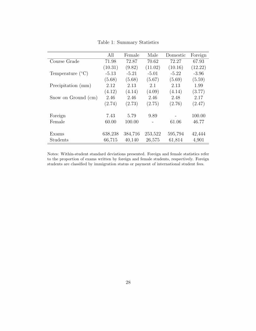
Table 1: Summary Statistics

All Female Male Domestic ForeignCourse Grade 71.98 72.87 70.62 72.27 67.93

(10.31) (9.82) (11.02) (10.16) (12.22)Temperature (◦C) -5.13 -5.21 -5.01 -5.22 -3.96

(5.68) (5.68) (5.67) (5.69) (5.59)Precipitation (mm) 2.12 2.13 2.1 2.13 1.99

(4.12) (4.14) (4.09) (4.14) (3.77)Snow on Ground (cm) 2.46 2.46 2.46 2.48 2.17

(2.74) (2.73) (2.75) (2.76) (2.47)

Foreign 7.43 5.79 9.89 - 100.00Female 60.00 100.00 - 61.06 46.77

Exams 638,238 384,716 253,522 595,794 42,444Students 66,715 40,140 26,575 61,814 4,901

Notes: Within-student standard deviations presented. Foreign and female statistics referto the proportion of exams written by foreign and female students, respectively. Foreignstudents are classified by immigration status or payment of international student fees.

28

Table 2: Temperature and Performance (Linear)

(1) (2) (3) (4) (5) (6)Z-Score Z-Score Z-Score Z-Score Z-Score Z-Score

PreferredTemperature (◦C) 0.833∗∗∗ 0.789∗∗∗ 0.699∗∗∗ 0.750∗∗∗ 0.742∗∗∗ 0.809∗∗∗

(0.043) (0.043) (0.045) (0.047) (0.047) (0.078)Precipitation Y Y Y Y Y YTemp × Precip Y Y Y Y Y YDay of Week FE Y Y Y Y YDate in Month Y Y Y YRelative Humidity Y Y YSnow on Ground Y YWindchill YExams 638238 638238 638238 638238 638238 638238Students 66715 66715 66715 66715 66715 66715

The dependent variable is hundredths of a standard deviation in final exam grade. The primaryindependent variable is exam day average temperature in degrees Celsius. All specifications in-clude year fixed effects. Within-student fixed effects model. Heteroskedasticity robust standarderrors are in parentheses, clustered at the student level. The sample comprises all exams writtenin December from 2007-2015. (*** p<0.01, ** p<0.05, * p<0.1.)

29

Table 3: Temperature and Performance (Non-linear)

(1) (2) (3) (4) (5) (6)Z-Score Z-Score Z-Score Z-Score Z-Score Z-Score

Preferred-15◦C 7.670∗∗∗ 4.621∗∗∗ 4.376∗∗∗ 4.091∗∗∗ 4.300∗∗∗ 3.782∗∗∗

(1.091) (1.119) (1.120) (1.123) (1.124) (1.161)-12.5◦C -2.887∗∗ -6.465∗∗∗ -6.760∗∗∗ -6.729∗∗∗ -6.651∗∗∗ -7.374∗∗∗

(1.354) (1.385) (1.387) (1.388) (1.387) (1.452)-10◦C 14.569∗∗∗ 10.651∗∗∗ 9.296∗∗∗ 8.853∗∗∗ 7.650∗∗∗ 6.756∗∗∗

(1.108) (1.126) (1.170) (1.175) (1.179) (1.296)-7.5◦C 11.446∗∗∗ 7.539∗∗∗ 6.755∗∗∗ 6.377∗∗∗ 3.870∗∗∗ 2.479∗

(1.140) (1.189) (1.205) (1.210) (1.227) (1.497)-5◦C 15.080∗∗∗ 11.653∗∗∗ 11.101∗∗∗ 11.522∗∗∗ 10.807∗∗∗ 9.362∗∗∗

(1.160) (1.167) (1.175) (1.185) (1.186) (1.472)-2.5◦C 16.067∗∗∗ 13.886∗∗∗ 13.020∗∗∗ 13.511∗∗∗ 13.358∗∗∗ 11.565∗∗∗

(1.080) (1.088) (1.105) (1.118) (1.118) (1.557)0◦C 16.788∗∗∗ 14.983∗∗∗ 13.423∗∗∗ 13.875∗∗∗ 14.170∗∗∗ 12.213∗∗∗

(1.214) (1.248) (1.297) (1.309) (1.308) (1.771)2.5◦C 35.063∗∗∗ 33.134∗∗∗ 30.633∗∗∗ 30.903∗∗∗ 32.970∗∗∗ 30.877∗∗∗

(1.637) (1.665) (1.760) (1.763) (1.772) (2.184)Precipitation Y Y Y Y Y YTemp × Precip Y Y Y Y Y YDay of Week FE Y Y Y Y YDate in Month Y Y Y YRelative Humidity Y Y YSnow on Ground Y YWindchill YExams 638238 638238 638238 638238 638238 638238Students 66715 66715 66715 66715 66715 66715

The dependent variable is hundredths of a standard deviation in final exam grade. The primary inde-pendent variables are exam day average temperature bins 2.5 degrees Celsius wide. The reference binis exam days with temperatures below -15◦C. Each bin is separately interacted with precipitation. Allspecifications include year fixed effects. Within-student fixed effects model. Heteroskedasticity robuststandard errors are in parentheses, clustered at the student level. The sample comprises all exams writ-ten in December from 2007-2015. (*** p<0.01, ** p<0.05, * p<0.1.)

30

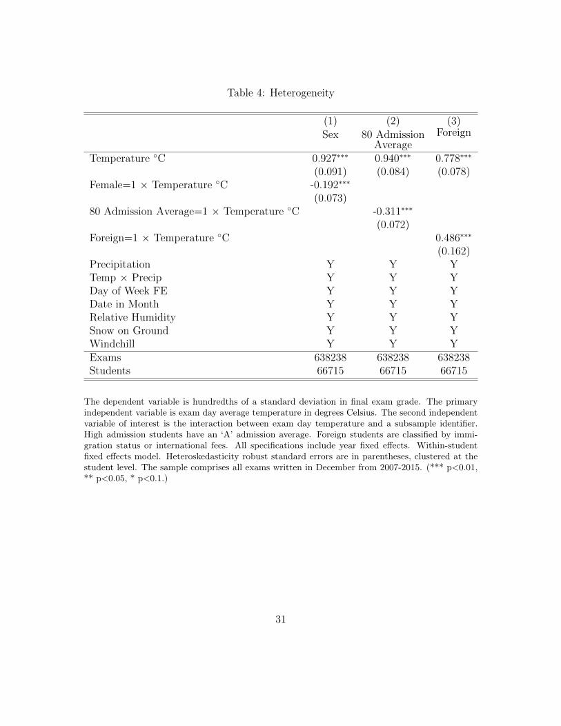
Table 4: Heterogeneity

(1) (2) (3)Sex 80 Admission

AverageForeign

Temperature ◦C 0.927∗∗∗ 0.940∗∗∗ 0.778∗∗∗

(0.091) (0.084) (0.078)Female=1 × Temperature ◦C -0.192∗∗∗

(0.073)80 Admission Average=1 × Temperature ◦C -0.311∗∗∗

(0.072)Foreign=1 × Temperature ◦C 0.486∗∗∗

(0.162)Precipitation Y Y YTemp × Precip Y Y YDay of Week FE Y Y YDate in Month Y Y YRelative Humidity Y Y YSnow on Ground Y Y YWindchill Y Y YExams 638238 638238 638238Students 66715 66715 66715

The dependent variable is hundredths of a standard deviation in final exam grade. The primaryindependent variable is exam day average temperature in degrees Celsius. The second independentvariable of interest is the interaction between exam day temperature and a subsample identifier.High admission students have an ‘A’ admission average. Foreign students are classified by immi-gration status or international fees. All specifications include year fixed effects. Within-studentfixed effects model. Heteroskedasticity robust standard errors are in parentheses, clustered at thestudent level. The sample comprises all exams written in December from 2007-2015. (*** p<0.01,** p<0.05, * p<0.1.)

31

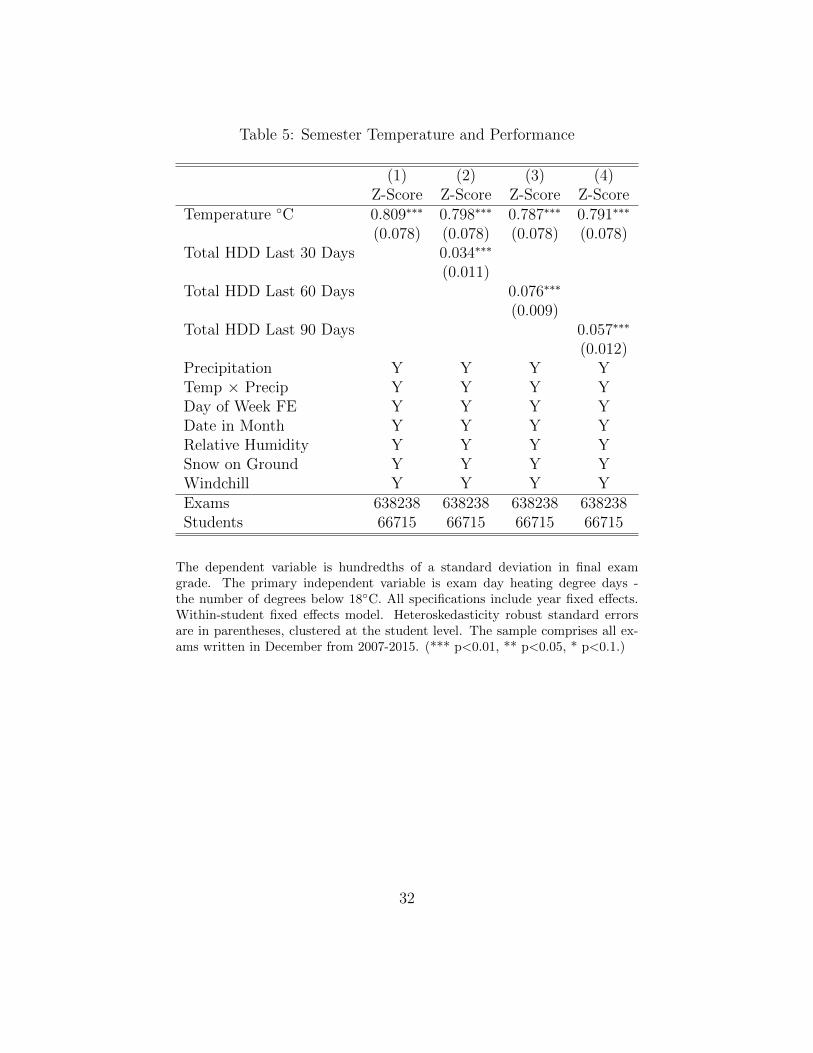
Table 5: Semester Temperature and Performance

(1) (2) (3) (4)Z-Score Z-Score Z-Score Z-Score

Temperature ◦C 0.809∗∗∗ 0.798∗∗∗ 0.787∗∗∗ 0.791∗∗∗

(0.078) (0.078) (0.078) (0.078)Total HDD Last 30 Days 0.034∗∗∗

(0.011)Total HDD Last 60 Days 0.076∗∗∗

(0.009)Total HDD Last 90 Days 0.057∗∗∗

(0.012)Precipitation Y Y Y YTemp × Precip Y Y Y YDay of Week FE Y Y Y YDate in Month Y Y Y YRelative Humidity Y Y Y YSnow on Ground Y Y Y YWindchill Y Y Y YExams 638238 638238 638238 638238Students 66715 66715 66715 66715

The dependent variable is hundredths of a standard deviation in final examgrade. The primary independent variable is exam day heating degree days -the number of degrees below 18◦C. All specifications include year fixed effects.Within-student fixed effects model. Heteroskedasticity robust standard errorsare in parentheses, clustered at the student level. The sample comprises all ex-ams written in December from 2007-2015. (*** p<0.01, ** p<0.05, * p<0.1.)

32

Table 6: Climate Control

(1) (2) (3)New BuildingInteraction 1

New BuildingInteraction 2

ExcludeLeaky Rooms

Temperature (◦C) 0.837∗∗∗ 0.795∗∗∗ 0.628∗∗∗

(0.081) (0.081) (0.086)New Building=1 -5.825∗∗∗ -5.661∗∗∗ -3.517∗∗∗

(0.507) (0.507) (0.527)New Building=1 × Temperature (◦C) -0.113∗ -0.136∗∗ -0.031

(0.061) (0.061) (0.063)Course Level FE Y YPrecipitation Y Y YTemp × Precip Y Y YYear FE Y Y YDay of Week FE Y Y YDate in Month Y Y YRelative Humidity Y Y YSnow on Ground Y Y YWindchill Y Y YExams 638238 638238 587030Students 66715 66715 66615

The dependent variable is hundredths of a standard deviation in final exam grade. The primary inde-pendent variable is exam day average temperature in degrees Celsius. The secondary variable of interestis the interaction between a new building (completed after or during 2000 C.E.). Leaky rooms have in-ternal temperature readings outside a ± 1◦C tolerance band. All specifications include year fixed effects.Within-student fixed effects model. Heteroskedasticity robust standard errors are in parentheses, clus-tered at the student level. The sample comprises all exams written in December from 2007-2015. (***p<0.01, ** p<0.05, * p<0.1.)

33

Table 7: Travel to Work

(1) (2) (3)All Movers ≤10km

Non-MoversTemperature (◦C) 0.719∗∗∗ 0.782∗∗∗ 0.866∗∗∗

(0.081) (0.236) (0.288)Distance (km) -0.003 -0.002

(0.004) (0.004)Temperature (◦C) × Distance (km) 0.000 0.000 -0.025

(0.000) (0.000) (0.036)Precipitation (mm) -0.437∗∗∗ -0.438∗∗∗ -0.980∗∗∗

(0.060) (0.170) (0.297)Temperature (◦C) × Precipitation (mm) -0.103∗∗∗ -0.095∗∗∗ -0.121∗∗∗

(0.010) (0.032) (0.025)Distance (km) × Precipitation (mm) -0.000 -0.000 0.084∗

(0.000) (0.000) (0.044)Snow on Ground (cm) -0.513∗∗∗ -0.631∗∗∗ -0.161

(0.054) (0.161) (0.232)Distance (km) × Snow on Ground (cm) 0.000 -0.000 -0.043

(0.000) (0.000) (0.032)Day of Week FE Y Y YDate in Month Y Y YRelative Humidity Y Y YWindchill Y Y YExams 598407 81347 107380Students 62596 8530 11514

The dependent variable is hundredths of a standard deviation in final exam grade. The pri-mary independent variable is exam day average temperature in degrees Celsius. The secondindependent variable of interest is the interaction between temperature and distance to stu-dent address (measured in km). Movers are students whose term address is different thantheir enrolment address. Students whose addresses are never more than 50km from campus.All specifications include year fixed effects. Within-student fixed effects model. Heteroskedas-ticity robust standard errors are in parentheses, clustered at the student level. The samplecomprises all exams written in December from 2007-2015. (*** p<0.01, ** p<0.05, * p<0.1.)

34

Table 8: Travel to Work (Subsamples)

(1) (2) (3) (4)≤2km ≤5km ≤10km ≤20km

Temperature (◦C) 0.919∗ 0.725∗∗ 0.770∗∗∗ 0.834∗∗∗

(0.532) (0.359) (0.214) (0.174)Precipitation Y Y Y YTemp × Precip Y Y Y YDay of Week FE Y Y Y YDate in Month Y Y Y YRelative Humidity Y Y Y YSnow on Ground Y Y Y YWindchill Y Y Y YExams 14182 31379 88217 113229Students 1966 3699 9771 11618

The dependent variable is hundredths of a standard deviation in finalexam grade. The primary independent variable is exam day averagetemperature in degrees Celsius. Each column header indicates the outerradius of successively distant donut-shaped regions. The second col-umn estimates our effect for addresses 2.0 km to 5.0 km from campus.All specifications include year fixed effects. Within-student fixed effectsmodel. Heteroskedasticity robust standard errors are in parentheses,clustered at the student level. The sample comprises all exams writtenin December from 2007-2015. (*** p<0.01, ** p<0.05, * p<0.1.)

35

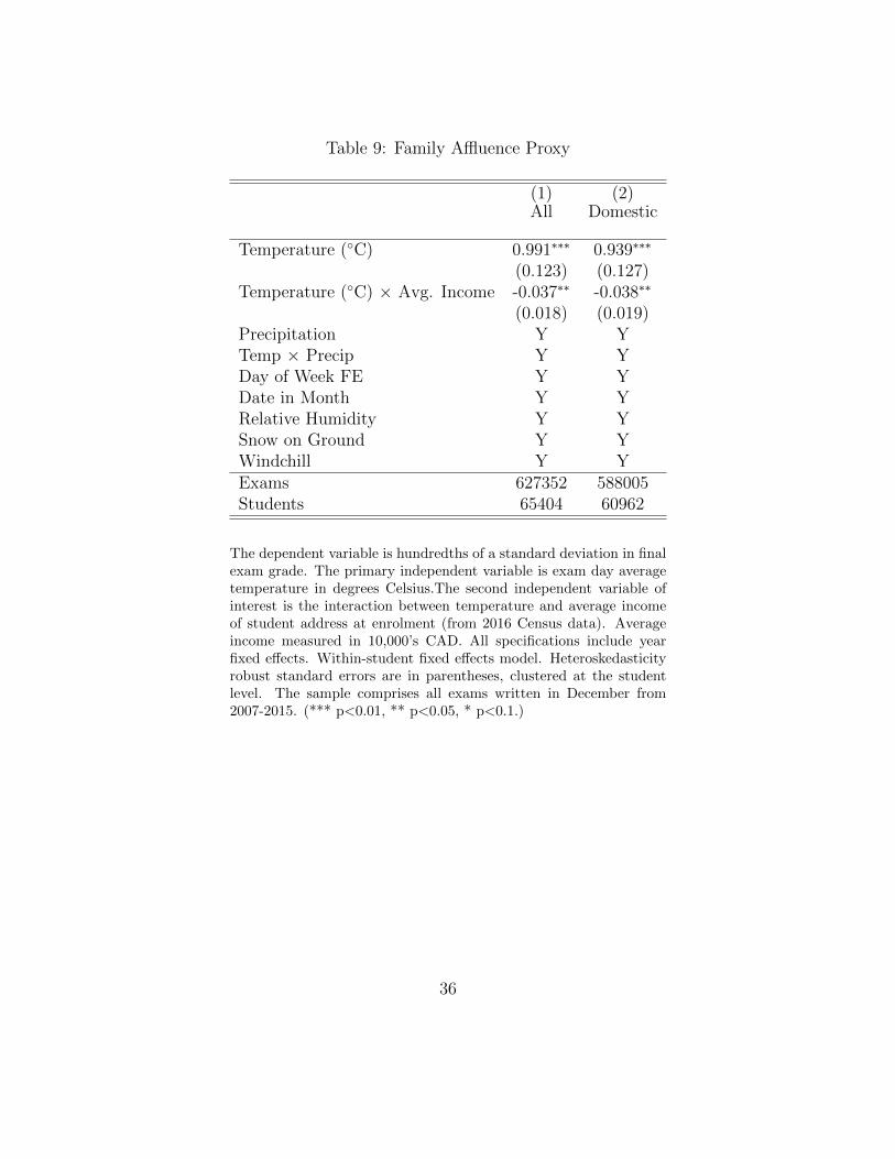
Table 9: Family Affluence Proxy

(1) (2)All Domestic

Temperature (◦C) 0.991∗∗∗ 0.939∗∗∗

(0.123) (0.127)Temperature (◦C) × Avg. Income -0.037∗∗ -0.038∗∗

(0.018) (0.019)Precipitation Y YTemp × Precip Y YDay of Week FE Y YDate in Month Y YRelative Humidity Y YSnow on Ground Y YWindchill Y YExams 627352 588005Students 65404 60962

The dependent variable is hundredths of a standard deviation in finalexam grade. The primary independent variable is exam day averagetemperature in degrees Celsius.The second independent variable ofinterest is the interaction between temperature and average incomeof student address at enrolment (from 2016 Census data). Averageincome measured in 10,000’s CAD. All specifications include yearfixed effects. Within-student fixed effects model. Heteroskedasticityrobust standard errors are in parentheses, clustered at the studentlevel. The sample comprises all exams written in December from2007-2015. (*** p<0.01, ** p<0.05, * p<0.1.)

36

Table 10: Heterogeneity Among Arrivees

(1) (2) (3) (4)Method 1

Probably HotMethod 1

OtherMethod 2

Probably HotMethod 2

OtherTemperature (◦C) 4.591∗∗∗ 1.226∗∗∗ 2.992∗∗∗ 1.495∗∗∗

(1.048) (0.401) (0.796) (0.425)Precipitation Y Y Y YTemp × Precip Y Y Y YDay of Week FE Y Y Y YDate in Month Y Y Y YRelative Humidity Y Y Y YSnow on Ground Y Y Y YWindchill Y Y Y YExams 6308 36136 9907 32537Students 985 3916 1275 3626

The dependent variable is hundredths of a standard deviation in final exam grade. Theprimary independent variable is exam day average temperature in degrees Celsius. Thefirst column estimates the preferred specification on international students who take all oftheir courses in French. The second column estimates our preferred specification on inter-national students who took none (N=3,085), or some fraction of their studies (N=981) inFrench. In the third and fourth column we relax our definition of probably hot country stu-dents to those who take all of their first year courses in French. All specifications includeyear fixed effects. Within-student fixed effects model. Heteroskedasticity robust standarderrors are in parentheses, clustered at the student level. The sample comprises all examswritten in December from 2007-2015. (*** p<0.01, ** p<0.05, * p<0.1.)

37

Table 11: Adaptation of Arrivees Over Time

(1) (2) (3) (4)All

(Year 1 Exams)Graduates

(Year 1 Exams) All GraduatesTemperature (◦C) 1.124∗∗∗ 0.498∗∗∗ 0.695∗∗∗ 0.358∗∗∗

(0.129) (0.163) (0.087) (0.098)Foreign=1 × Temperature (◦C) 0.855∗∗∗ 1.300∗∗∗ 0.866∗∗∗ 1.100∗∗∗

(0.318) (0.452) (0.252) (0.326)Temperature (◦C) × Years Enrolled 0.022 0.035

(0.031) (0.033)Foreign=1 × Temperature (◦C) × Years Enrolled -0.237∗ -0.394∗∗

(0.139) (0.159)Course Level FE Y Y Y YPrecipitation Y Y Y YTemp × Precip Y Y Y YDay of Week FE Y Y Y YDate in Month Y Y Y YRelative Humidity Y Y Y YSnow on Ground Y Y Y YWindchill Y Y Y YExams 265804 136319 638238 426583Students 66447 33228 66715 33322

The dependent variable is hundredths of a standard deviation in final exam grade. The primary independent variable is exam dayaverage temperature in degrees Celsius. All specifications include course-level fixed effects (e.g. 2000 level courses). Years enrolledbegins at 0 for the first winter of exams, and typically ends at 3 years. In columns 1 and 2, we estimate only on the first year’scourse results and do not include year fixed effects. Columns 3 and 4 include year fixed effects. Within-student fixed effects model.Heteroskedasticity robust standard errors are in parentheses, clustered at the student level. The sample comprises all exams writtenin December from 2007-2015. (*** p<0.01, ** p<0.05, * p<0.1.)

38

Table 12: Robustness

(1) (2) (3) (4) (5) (6) (7) (8)Mean Temp(Preferred)

24 HourAverage

MinTemp

ExamTemp

NextStation

Winsorizedat 10%

DryDays

NoControls

Temp. Measure 0.809∗∗∗ 0.771∗∗∗ 0.386∗∗∗ 0.603∗∗∗ 0.532∗∗∗ 0.724∗∗∗ 0.963∗∗∗ 1.526∗∗∗

(0.078) (0.080) (0.064) (0.095) (0.075) (0.094) (0.128) (0.035)Precipitation Y Y Y Y Y YTemp × Precip Y Y Y Y Y YDay of Week FE Y Y Y Y Y Y YDate in Month Y Y Y Y Y Y YRelative Humidity Y Y Y Y Y Y YSnow on Ground Y Y Y Y Y Y YWindchill Y Y Y Y Y Y YMean of Measure -5.14 -4.76 -8.68 -4.16 -5.3 -5.12 -6.64 -5.14SD of Measure 6.61 6.45 7.51 6.52 6.75 5.52 6.66 6.61Exams 638238 638238 638238 638238 638238 638238 288717 638238Students 66715 66715 66715 66715 66715 66715 64016 66715

The dependent variable is hundredths of a standard deviation in final exam grade. Each column title denotes the primary indepen-dent variable. The first column is average exam day temperature in degrees Celsius, calculated as the average of daily maximum andminimum. The second column is the 24 hour equally weighted average temperature. The third column uses daily minimum temper-ature. The fourth column uses the average hourly temperature during the 3 hour window of the exam. The fifth column uses dailyaverage temperature from the next-closest weather station (an international airport approximately 14km away). The sixth usestemperatures winsorized at the 10% and 90% level. The seventh column estimates the preferred specification only on days withoutprecipitation. The eighth column simply regresses performance and temperature. Other than ‘no controls’, all specifications in-clude year fixed effects. Within-student fixed effects model. Heteroskedasticity robust standard errors are in parentheses, clusteredat the student level. The sample comprises all exams written in December from 2007-2015. (*** p<0.01, ** p<0.05, * p<0.1.)

39

Table 13: Alternative Standard Errors

(1) (2) (3) (4)PreferredStudent Unclustered

Cohort(Bootstrap) Exam Ventiles

Temperature (◦C) 0.809∗∗∗ 0.809∗∗∗ 0.809∗∗∗ 0.809∗∗∗

(0.078) (0.078) (0.252) (0.225)Precipitation Y Y Y YTemp × Precip Y Y Y YDay of Week FE Y Y Y YDate in Month Y Y Y YRelative Humidity Y Y Y YSnow on Ground Y Y Y YWindchill Y Y Y YExams 638238 638238 638238 638238Clusters 66715 9 20

The dependent variable is hundredths of a standard deviation in final exam grade. The pri-mary independent variable is exam day average temperature in degrees Celsius. (1) errorsclustered at the student level (2) unclustered errors (3) bootstrapped errors clustered by co-hort (4) ventiles of average exam temperatures. All specifications include year fixed effects.Within-student fixed effects model. The sample comprises all exams written in Decemberfrom 2007-2015. (*** p<0.01, ** p<0.05, * p<0.1.)

40

Figure 1: Distribution of Temperature Treatments

In this figure, we plot the percentage of exams written on days with average temperatures divided into 2 degree Celsius bins.Each exam, rather than each exam day, represents a single observation.

41

Figure 2: Temperature and Performance (Only Year Controls)

In this figure, we plot the imputed residual exam grade (after accounting for year fixed effects) by exam day temperature.Temperature is rounded to the nearest 0.5◦C. Markers are sized proportional to number of observations they represent.

42

Figure 3: Temperature and Performance (Non-Linear)

In this figure, we present the estimated coefficients by “binning” daily temperatures into 2.5◦C intervals. The referencecategory is exams written with daily temperatures below -15◦C. The dependent variable is exam score standard deviationsin hundredths. The left panel corresponds to a parsimonious specification with student and year fixed effects, precipitation,and its interaction with each temperature bin. The right panel corresponds to our preferred specification with additionalcontrols. Whiskers indicate the 95% confidence level.

43

Figure 4: Indoor and Outdoor Temperatures (MNT021)

In this figure, we plot the outdoor temperatures realized during 2018 December exams and the internal temperature variationsfrom room average in the largest exam room by contribution to sample. We fit a regression line with slope coefficient of0.0003 and an associated t-statistic of 0.10. Reference lines are provided at 1◦C (above) and -1◦C (below) room average.

44

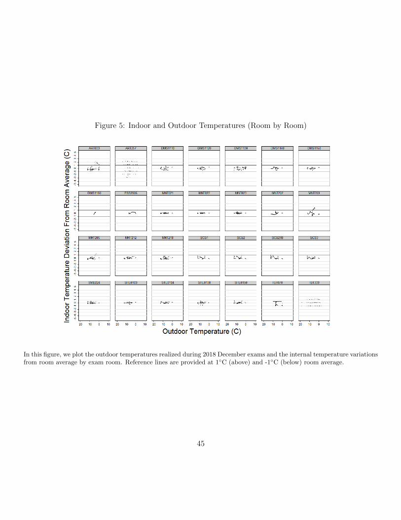
Figure 5: Indoor and Outdoor Temperatures (Room by Room)

In this figure, we plot the outdoor temperatures realized during 2018 December exams and the internal temperature variationsfrom room average by exam room. Reference lines are provided at 1◦C (above) and -1◦C (below) room average.

45

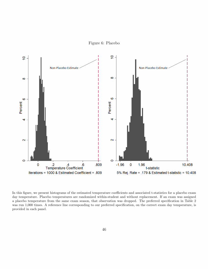
Figure 6: Placebo

In this figure, we present histograms of the estimated temperature coefficients and associated t-statistics for a placebo examday temperature. Placebo temperatures are randomized within-student and without replacement. If an exam was assigneda placebo temperature from the same exam season, that observation was dropped. The preferred specification in Table 2was run 1,000 times. A reference line corresponding to our preferred specification, on the correct exam day temperature, isprovided in each panel.

46

Appendices

Table A1: Temperature and Performance (Linear)

(1) (2) (3) (4) (5) (6) (7) (8)Z-Score Z-Score Z-Score Z-Score Z-Score Z-Score Z-Score Z-Score

PreferredTemperature (◦C) 0.609∗∗∗ 0.688∗∗∗ 0.833∗∗∗ 0.789∗∗∗ 0.699∗∗∗ 0.750∗∗∗ 0.742∗∗∗ 0.809∗∗∗

(0.040) (0.042) (0.043) (0.043) (0.045) (0.047) (0.047) (0.078)Precipitation -0.387∗∗∗ -0.712∗∗∗ -0.451∗∗∗ -0.425∗∗∗ -0.355∗∗∗ -0.419∗∗∗ -0.425∗∗∗

(0.046) (0.050) (0.052) (0.052) (0.055) (0.055) (0.055)Temp × Precip -0.128∗∗∗ -0.117∗∗∗ -0.107∗∗∗ -0.112∗∗∗ -0.105∗∗∗ -0.104∗∗∗

(0.010) (0.010) (0.010) (0.010) (0.010) (0.010)Date in Month -0.353∗∗∗ -0.315∗∗∗ -0.015 -0.013

(0.053) (0.054) (0.062) (0.062)Relative Humidity -0.077∗∗∗ -0.025 -0.019

(0.019) (0.019) (0.020)Snow on Ground -0.500∗∗∗ -0.503∗∗∗

(0.051) (0.051)Windchill -0.037

(0.034)Day of Week FE Y Y Y Y YYear FE Y Y Y Y Y Y Y YExams 638238 638238 638238 638238 638238 638238 638238 638238Students 66715 66715 66715 66715 66715 66715 66715 66715

The dependent variable is hundredths of a standard deviation in final exam grade. The primary independent variable is examday average temperature in degrees Celsius. All specifications include year fixed effects. Within-student fixed effects model.Heteroskedasticity robust standard errors are in parentheses, clustered at the student level. The sample comprises all examswritten in December from 2007-2015. (*** p<0.01, ** p<0.05, * p<0.1.)

47

Table A2: Temperature and Performance (Deciles)

(1) (2) (3) (4) (5) (6)Z-Score Z-Score Z-Score Z-Score Z-Score Z-Score

Preferred-14.7◦C 6.805∗∗∗ 4.484∗∗∗ 4.277∗∗∗ 3.796∗∗∗ 2.916∗∗∗ 1.733

(1.030) (1.051) (1.052) (1.057) (1.061) (1.117)-10.6◦C 8.666∗∗∗ 3.514∗∗∗ 1.960∗ 1.376 -1.192 -3.243∗∗

(1.113) (1.148) (1.168) (1.171) (1.206) (1.363)-8.3◦C 18.341∗∗∗ 14.276∗∗∗ 12.494∗∗∗ 11.755∗∗∗ 9.297∗∗∗ 6.572∗∗∗

(1.075) (1.102) (1.131) (1.138) (1.170) (1.431)-6.5◦C 8.474∗∗∗ 5.319∗∗∗ 5.282∗∗∗ 5.113∗∗∗ 3.070∗∗ -0.023

(1.211) (1.234) (1.234) (1.234) (1.256) (1.585)-4.1◦C 19.629∗∗∗ 12.205∗∗∗ 11.748∗∗∗ 12.589∗∗∗ 12.015∗∗∗ 8.621∗∗∗

(1.317) (1.355) (1.358) (1.367) (1.368) (1.715)-2.7◦C 11.557∗∗∗ 7.405∗∗∗ 5.992∗∗∗ 6.711∗∗∗ 5.041∗∗∗ 1.005

(1.127) (1.137) (1.155) (1.163) (1.177) (1.702)-.7◦C 17.268∗∗∗ 14.313∗∗∗ 13.270∗∗∗ 14.719∗∗∗ 13.635∗∗∗ 9.348∗∗∗

(1.184) (1.199) (1.208) (1.240) (1.244) (1.802).3◦C 15.850∗∗∗ 14.862∗∗∗ 12.868∗∗∗ 13.693∗∗∗ 12.730∗∗∗ 8.327∗∗∗

(1.208) (1.245) (1.275) (1.287) (1.291) (1.862)2.2◦C 27.861∗∗∗ 23.528∗∗∗ 20.719∗∗∗ 21.947∗∗∗ 21.914∗∗∗ 17.239∗∗∗

(1.534) (1.574) (1.627) (1.649) (1.649) (2.182)Precipitation Y Y Y Y Y YTemp × Precip Y Y Y Y Y YDay of Week FE Y Y Y Y YDate in Month Y Y Y YRelative Humidity Y Y YSnow on Ground Y YWindchill YExams 638238 638238 638238 638238 638238 638238Students 66715 66715 66715 66715 66715 66715

The dependent variable is hundredths of a standard deviation in final exam grade. The primary inde-pendent variables are exam day average temperature deciles. The reference bin is exam days with tem-peratures below -14.7◦C. Each bin is separately interacted with precipitation. All specifications includeyear fixed effects. Within-student fixed effects model. Heteroskedasticity robust standard errors are inparentheses, clustered at the student level. The sample comprises all exams written in December from2007-2015. (*** p<0.01, ** p<0.05, * p<0.1.)

48

Table A3: Semester Temperature and Performance

(1) (2) (3) (4) (5) (6) (7)Z-Score Z-Score Z-Score Z-Score Z-Score Z-Score Z-Score

Temperature (◦C) 0.809∗∗∗ 0.796∗∗∗ 0.964∗∗∗ 0.839∗∗∗ 0.798∗∗∗ 0.786∗∗∗ 0.803∗∗∗

(0.078) (0.091) (0.083) (0.080) (0.078) (0.078) (0.078)Avg. Temp. Last 1 Days 0.017

(0.058)Avg. Temp. Last 3 Days -0.307∗∗∗

(0.065)Avg. Temp. Last 5 Days -0.108

(0.080)Avg. Temp. Last 30 Days -1.028∗∗∗

(0.318)Avg. Temp. Last 60 Days -4.580∗∗∗

(0.559)Avg. Temp. Last 90 Days -4.395∗∗∗

(1.152)Precipitation Y Y Y Y Y Y YTemp × Precip Y Y Y Y Y Y YDay of Week FE Y Y Y Y Y Y YDate in Month Y Y Y Y Y Y YRelative Humidity Y Y Y Y Y Y YSnow on Ground Y Y Y Y Y Y YWindchill Y Y Y Y Y Y YExams 638238 638238 638238 638238 638238 638238 638238Students 66715 66715 66715 66715 66715 66715 66715

The dependent variable is hundredths of a standard deviation in final exam grade. The primary independent variable isexam day temperature. The secondary independent variable is average temperature leading up to exam day. All speci-fications include year fixed effects. Within-student fixed effects model. Heteroskedasticity robust standard errors are inparentheses, clustered at the student level. The sample comprises all exams written in December from 2007-2015. (***p<0.01, ** p<0.05, * p<0.1.)

49

Table A4: Temperature and Performance, Alternative Standardization

(1) (2) (3) (4) (5) (6)Z-Score Z-Score Z-Score Z-Score Z-Score Z-Score

PreferredTemperature (◦C) 0.085∗∗ 0.074∗ 0.081∗ 0.091∗∗ 0.093∗∗ 0.137∗

(0.042) (0.043) (0.045) (0.046) (0.046) (0.077)Precipitation Y Y Y Y Y YTemp × Precip Y Y Y Y Y YDay of Week FE Y Y Y Y YDate in Month Y Y Y YRelative Humidity Y Y YSnow on Ground Y YWindchill YExams 637988 637988 637988 637988 637988 637988Students 66711 66711 66711 66711 66711 66711

The dependent variable is hundredths of a standard deviation in final exam grade, standardizedby year and course. The primary independent variable is exam day average temperature in de-grees Celsius. All specifications include year fixed effects. Within-student fixed effects model.Heteroskedasticity robust standard errors are in parentheses, clustered at the student level. Thesample comprises all exams written in December from 2007-2015. (*** p<0.01, ** p<0.05, *p<0.1.)

50

Figure A1: Temperature and Performance (Deciles)

In this figure, we present the estimated coefficients for indicator variables created by assigning daily temperatures into decileintervals. The reference category is exams written in the 10% coldest daily average temperatures. The dependent variable isexam score standard deviations in hundredths. The left panel corresponds to a parsimonious specification with student andyear fixed effects, precipitation, and its interaction with each temperature bin. The right panel corresponds to our preferredspecification with additional controls. Whiskers indicate the 95% confidence level.

51

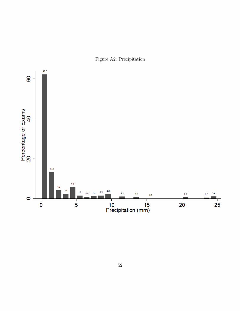
Figure A2: Precipitation

52

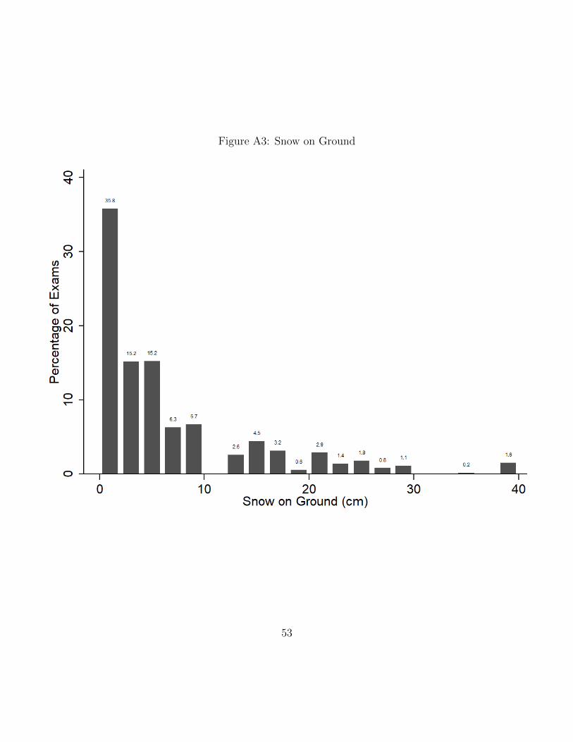
Figure A3: Snow on Ground

53

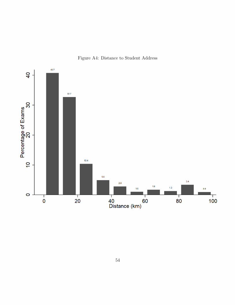
Figure A4: Distance to Student Address

54

Figure A5: Student Application Address Average Income

55