Brain Connectivity in Positive and Negative SyndromeSchizophrenia

T. Medkoura, A. T. Waldena,∗, A. P. Burgessb, V. B. Streletsc

aDepartment of Mathematics, Imperial College London, 180 Queen’s Gate, London SW72BZ, UK

bAston University School of Life and Health Sciences, Aston Triangle, Birmingham B47ET, UK

cInstitute of Higher Nervous Activity and Neurophysiology, Russian Academy of Sciences,Butlerov Street 5 A, 117485 Moscow, Russia

Abstract

If, as is widely believed, schizophrenia is characterised by abnormalities of

brain functional connectivity, then it seems reasonable to expect that differ-

ent subtypes of schizophrenia could be discriminated in the same way. How-

ever, evidence for differences in functional connectivity between the subtypes of

schizophrenia is largely lacking and, where it exists, it could be accounted for by

clinical differences between the patients (e.g. medication) or by the limitations

of the measures used. In this study, we measured EEG functional connectivity in

unmedicated male patients diagnosed with either positive or negative syndrome

schizophrenia and compared them with age and sex matched healthy controls.

Using new methodology (Medkour et al., 2009) based on partial coherence, brain

connectivity plots were constructed for positive and negative syndrome patients

and controls. Reliable differences in the pattern of functional connectivity were

found with both syndromes showing not only an absence of some of the con-

nections that were seen in controls but also the presence of connections that

the controls did not show. Comparing connectivity graphs using the Hamming

distance, the negative-syndrome patients were found to be more distant from

the controls than were the positive syndrome patients. Bootstrap distributions

∗Corresponding author. Tel: (0)20 7594 8524; Fax: (0)20 7594 8517; e-mail:a.walden@imperial.ac.uk

Preprint submitted to Neuroscience June 8, 2010

of these distances were created which showed a significant difference in the mean

distances that was consistent with the observation that negative-syndrome di-

agnosis is associated with a more severe form of schizophrenia. We conclude

that schizophrenia is characterised by widespread changes in functional con-

nectivity with negative syndrome patients showing a more extreme pattern of

abnormality than positive syndrome patients.

Key words: Brain connectivity, Graphical models, Partial spectral coherence,

Schizophrenia

Introduction

Bleuler’s original conception of schizophrenia as a disease caused by discon-

nections between the fundamental components of the mind has, after a long

hibernation, undergone a process of revival and modernisation and been re-

framed in terms of an abnormality of functional connectivity in the brain (Fris-

ton and Frith, 1995). So successful has this revival been that the disconnection

hypothesis has become one of the most active areas of schizophrenia research

(Bullmore and Fletcher, 2003). In part the renaissance of the disconnection hy-

pothesis can be viewed as a natural consequence of technological developments

that have made possible the measurement of both structural (Diffusion Tensor

Imaging) and functional connectivity in vivo. Perhaps more important, how-

ever, has been the growing understanding of the role of synchronous cerebral

oscillations as a neural code that enables visual feature binding and, by exten-

sion, permits functional integration across the brain more generally. From here,

it is but a small step to propose that schizophrenia should be characterised by

abnormalities in the pattern of synchronous cerebral oscillations and numerous

studies have been reported that set out to test this hypothesis.

There is certainly consistent evidence of abnormal cerebral oscillations in

schizophrenia. Patients typically show unusually high EEG power in the low

frequencies (delta and theta bands, < 8Hz) which is usually interpreted as evi-

dence of neurodevelopmental delay (Galderisi et al., 2009), but this difference is

2

by no means specific to schizophrenia (Coutin-Churchman et al., 2003). Further-

more, although EEG power at single scalp sites reflects localised synchronous

neuronal activity, it does not provide a useful index of more long-distance func-

tional connectivity and to do this, some measure of inter-channel covariation is

required, such as coherence or phase synchrony. Much of the early work on func-

tional connectivity in schizophrenia focussed on EEG coherence in the classical

frequency bands (delta, theta, alpha and beta) and although abnormalities were

claimed, the direction and locus of the changes reported were inconsistent (Leo-

cani and Comi, 1999). More recent studies, perhaps influenced by proposed

role of gamma oscillations in feature binding, have examined high frequency

connectivity using a plethora of measures of connectivity and but have come

to broadly similar conclusions (Stephan et al., 2006; Uhlhaas et al., 2008): al-

though there is consistent evidence for the aberrance of functional connectivity

mediated through cortical oscillations in schizophrenia, the nature and direction

of the abnormality is uncertain.

This confusing state of affairs may reflect the true heterogeneity of the disor-

der and the samples of patients examined. It might, however, reflect differences

between patients that arise secondary to the diagnosis of schizophrenia, such as

medication, rather than to the diversity of the disease itself. EEG measures of

functional connectivity also face fundamental methodological challenges that,

although well known, have not been adequately addressed. These include the

problems of volume conduction and that of multiple comparisons.

The problem of volume conduction is that if there is a significant level of

connectivity between two channels, is it due to a flow of information between

two or more spatially separate regions or because the sensors are detecting ac-

tivity emanating from a single source? Most measures of connectivity, including

coherence, phase synchrony and all current non-linear measures are unable to

discriminate between these alternatives which means that they are not true mea-

sures of connectivity at all. Some measures, such as imaginary coherence (Nolte

et al., 2004) or phase lag index (Stam et al., 2007) do successfully mitigate the

volume conduction issue but invariably underestimate the ‘true’ connectivity. If

3

it was possible to solve the inverse problem, then the volume conduction prob-

lem would become tractable but, unfortunately, source localisation can only be

‘solved’ by making strong assumptions about the nature of the sources to be

localised and these assumptions invariably affect the estimates of connectivity

between sources.

Medkour et al. (2009) developed a method for determining functional con-

nectivity from partial coherence. Among the attractive properties of partial co-

herence are that it makes no assumptions about the nature of cerebral sources

and markedly reduces the impact of volume conduction. Given these strengths,

it is not surprising that partial coherence has been used before in EEG research

but in all previous variants, the estimates of connectivity were unreliable. The

revised approach carefully considers issues such as spectral matrix inversion,

side-lobe leakage suppression, bias removal and multiple hypothesis testing for

dependent partial coherencies, all aimed at increasing the reliability of connec-

tivity results.

The clinical problems of the heterogeneity of schizophrenia and the impact of

pharmaceutical treatments on functional connectivity also make interpretation

of the studies problematic. The issue of medication is that any differences seen

between patients and controls might well be due to the psychotropic effects of

the medication rather than to the effects of the disease itself. The heterogeneity

of schizophrenia is widely recognised clinically and, although there is no con-

sensus, at least two syndromes are widely acknowledged: positive and negative

(Andreasen and Olsen, 1982). Relatively little work has attempted to validate

the positive/negative distinction using EEG but the finding that negative pa-

tients show greater delta and theta power than positive syndrome patients has

been consistently reported (Begic et al., 2000, 2009; E. R. John et al., 1994;

J. P. John et al., 2009). Furthermore, studies investigating Liddle’s 3-cluster

subtyping of schizophrenia has also found associations between delta power and

Liddle’s Psychomotor Poverty factor, which measures symptoms that are pre-

dominantly negative symptoms (Harris et al., 2001; Gross et al., 2006). Only

two studies have examined functional connectivity measures in this context and

4

both reported differences between positive and negative syndromes at high fre-

quencies (Strelets et al., 2002; Lee et al., 2003) with negative patients showing

lower levels of power.

The aim of this study was to determine whether it is possible to discriminate

between positive and negative schizophrenia using the new methods of Medkour

et al. (2009) — briefly discussed above, and referred to appropriately in what

follows — for the determination of EEG functional connectivity that overcome

many of the problems associated with previous approaches. New modelling and

bootstrap resampling steps are developed in the current paper. Because previous

research has found consistent differences at low frequencies, it was decided to

focus on the delta frequency range, [0.5, 4]Hz, using a sample of unmedicated

patients.

The paper is structured as follows. Firstly we discuss the subjects and

EEG data. For clarity, we then divide up our methodology and results into

three parts. Firstly, we give background details on the spectral matrix esti-

mation method, and partial coherence calculation, its debiassing, and use in

constructing a connectivity graph. Next we turn to defining the strength of

connections through a measure we call ‘total weighted relative strength,’ and

give a gamma distribution model for it. By using a threshold, this distribution

is used to construct a connectivity graph, represented by a connection vector

of ones and zeros. Finally, using the Hamming distance measure we show that,

over a range of thresholds, the graph for negative-syndrome patients is further

from the graph for controls than is the graph for positive-syndrome patients.

Bootstrap resampling shows that this finding is statistically significant.

Data

Subjects

The data sample (see also Strelets et al. (2002)) was acquired from 34 male

forensic patients (mean age 35; range 20-60) with a DSM-III-R diagnosis of

schizophrenia from the Serbsky Institute in Moscow. Of these patients, 15

5

showed a clear predominance of positive symptoms – delusions, hallucinations

(Andreasen, 1984) and 19 had negative symptoms – personality defect, emo-

tional retardation (Andreasen, 1983). (Patients with a mixed clinical picture

were omitted from the study.) All patients were medication free or withdrawn

from medication for at least 7 days before examination. The control group con-

sisted of 24 healthy volunteers of comparable age to the patients (mean age=

31; range 19-42). All subjects gave written informed consent for the investiga-

tion. Ethical approval came from the local Moscow ethics committee, and in

compliance with national legislation and the Declaration of Helsinki. We shall

denote the set of patients diagnosed as positive and negative syndromes by Pand N , respectively, and the controls by C.

EEG data and initial treatment

EEG was recorded using an MBM (Russia) EEG mapper from 10 scalp sites

(F3, F4, C3, C4, T3, T4, P3, P4, O1 and O2) referenced to linked ears with a

bandpass filter of 0.5-45Hz. EEG recordings were obtained for resting conditions

with eyes closed. A sampling rate of 100Hz, (sample interval ∆t = 0.01s),

was used so that the Nyquist frequency is fN = 1/(2∆t) = 50Hz. While

it would have been desirable to have more prefrontal and cortex sites, and a

higher sampling rate (enabling examination of the gamma band), these were

not available in this rare heritage clinical data set from unmedicated patients.

The alpha rhythm creates a characteristic and dominant spectral line at a

frequency of approximately 10Hz, (Dawson and Fischer, 1994). The mean of

a spectral estimator consists of the convolution of the true spectrum with a

spectral window which depends on the particular estimation method used (e.g.,

Percival and Walden, 1993). The window will have a main lobe and multiple

sidelobes and when the window is centred at the position of the spectral line,

these sidelobes will transfer power into other parts of the spectrum including

the delta band, even though the line is in the [8, 12]Hz alpha band. If the

line is sufficiently dominant, such side-lobe leakage will be noticeable and cause

serious estimation errors in the delta band. As a result of such considerations, we

6

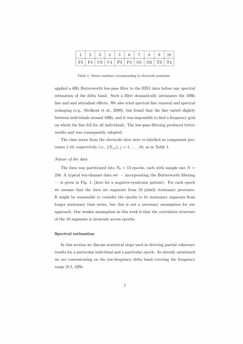
1 2 3 4 5 6 7 8 9 10

F3 F4 C3 C4 P3 P4 O1 O2 T3 T4

Table 1: Series numbers corresponding to electrode positions.

applied a 6Hz Butterworth low-pass filter to the EEG data before any spectral

estimation of the delta band. Such a filter dramatically attenuates the 10Hz

line and and attendant effects. We also tried spectral line removal and spectral

reshaping (e.g., Medkour et al., 2009), but found that the line varied slightly

between individuals around 10Hz, and it was impossible to find a frequency grid

on which the line fell for all individuals. The low-pass filtering produced better

results and was consequently adopted.

The time series from the electrode sites were re-labelled as component pro-

cesses 1-10, respectively, i.e., {Xj,t}, j = 1, . . . , 10, as in Table 1.

Nature of the data

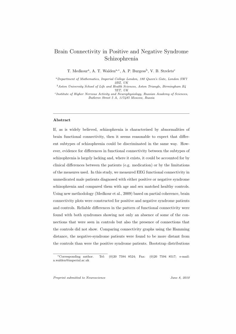
The data was partitioned into Nb = 13 epochs, each with sample size N =

256. A typical ten-channel data set — incorporating the Butterworth filtering

— is given in Fig. 1, (here for a negative-syndrome patient). For each epoch

we assume that the data are segments from 10 jointly stationary processes.

It might be reasonable to consider the epochs to be stationary segments from

longer stationary time series, but this is not a necessary assumption for our

approach. Our weaker assumption in this work is that the correlation structure

of the 10 segments is invariant across epochs.

Spectral estimation

In this section we discuss statistical steps used in deriving partial coherence

results for a particular individual and a particular epoch. As already mentioned

we are concentrating on the low-frequency delta band covering the frequency

range [0.5, 4]Hz.

7

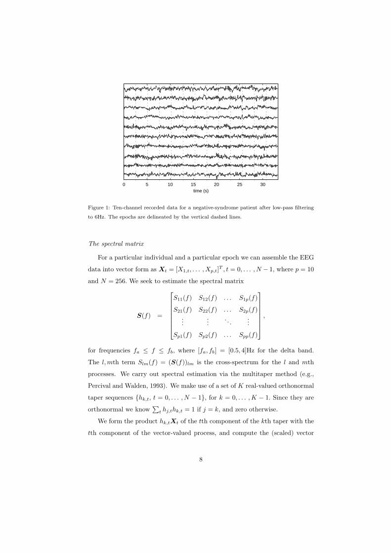
0 5 10 15 20 25 30time (s)

Figure 1: Ten-channel recorded data for a negative-syndrome patient after low-pass filtering

to 6Hz. The epochs are delineated by the vertical dashed lines.

The spectral matrix

For a particular individual and a particular epoch we can assemble the EEG

data into vector form as Xt = [X1,t, . . . , Xp,t]T , t = 0, . . . , N − 1, where p = 10

and N = 256. We seek to estimate the spectral matrix

S(f) =

S11(f) S12(f) . . . S1p(f)

S21(f) S22(f) . . . S2p(f)...

.... . .

...

Sp1(f) Sp2(f) . . . Spp(f)

,

for frequencies fa ≤ f ≤ fb, where [fa, fb] = [0.5, 4]Hz for the delta band.

The l, mth term Slm(f) = (S(f))lm is the cross-spectrum for the l and mth

processes. We carry out spectral estimation via the multitaper method (e.g.,

Percival and Walden, 1993). We make use of a set of K real-valued orthonormal

taper sequences {hk,t, t = 0, . . . , N − 1}, for k = 0, . . . , K − 1. Since they are

orthonormal we know∑

t hj,thk,t = 1 if j = k, and zero otherwise.

We form the product hk,tXt of the tth component of the kth taper with the

tth component of the vector-valued process, and compute the (scaled) vector

8

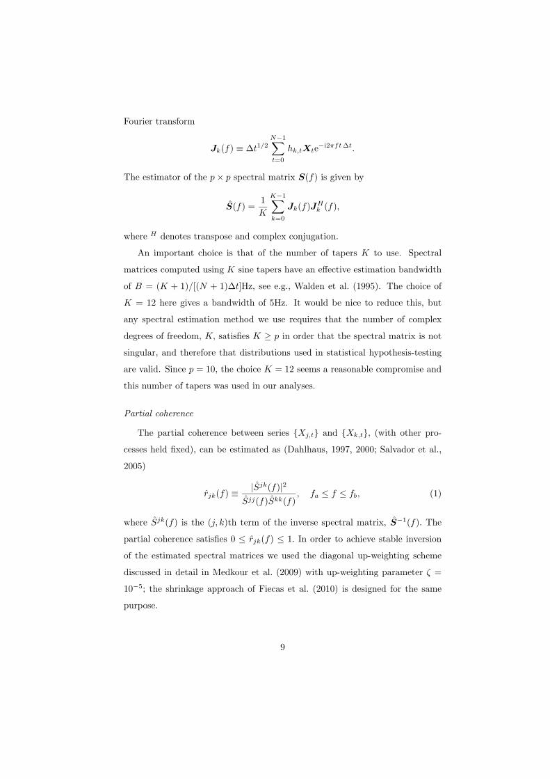
Fourier transform

Jk(f) ≡ ∆t1/2N−1∑t=0

hk,tXte−i2πft ∆t.

The estimator of the p × p spectral matrix S(f) is given by

S(f) =1K

K−1∑k=0

Jk(f)JHk (f),

where H denotes transpose and complex conjugation.

An important choice is that of the number of tapers K to use. Spectral

matrices computed using K sine tapers have an effective estimation bandwidth

of B = (K + 1)/[(N + 1)∆t]Hz, see e.g., Walden et al. (1995). The choice of

K = 12 here gives a bandwidth of 5Hz. It would be nice to reduce this, but

any spectral estimation method we use requires that the number of complex

degrees of freedom, K, satisfies K ≥ p in order that the spectral matrix is not

singular, and therefore that distributions used in statistical hypothesis-testing

are valid. Since p = 10, the choice K = 12 seems a reasonable compromise and

this number of tapers was used in our analyses.

Partial coherence

The partial coherence between series {Xj,t} and {Xk,t}, (with other pro-

cesses held fixed), can be estimated as (Dahlhaus, 1997, 2000; Salvador et al.,

2005)

rjk(f) ≡ |Sjk(f)|2

Sjj(f)Skk(f), fa ≤ f ≤ fb, (1)

where Sjk(f) is the (j, k)th term of the inverse spectral matrix, S−1(f). The

partial coherence satisfies 0 ≤ rjk(f) ≤ 1. In order to achieve stable inversion

of the estimated spectral matrices we used the diagonal up-weighting scheme

discussed in detail in Medkour et al. (2009) with up-weighting parameter ζ =

10−5; the shrinkage approach of Fiecas et al. (2010) is designed for the same

purpose.

9

In order to debias the raw estimated partial coherence we note the follow-

ing. The statistical properties of the partial coherence estimator are those of

ordinary coherence provided the degrees of freedom K in ordinary coherence

are replaced by K − p + 2 for partial coherence. Making this adjustment in

Benignus’s formula (Benignus, 1969) for debiassing of ordinary coherence, we

see that partial coherence can be debiassed by using

rjk(f) =rjk(f) − 1

K−p+2

1 − 1K−p+2

.

For K = 12 and p = 10 a debiased version of the estimated partial coherence is

thus given by

rjk(f) =43rjk(f) − 1

3. (2)

The formula (2) is used throughout this work when referring to the estimated

partial coherence, apart from in hypothesis tests where of course the raw esti-

mator is used since it is the distribution of the raw estimator which is known

and utilised in the tests.

Partial coherence and conditional correlation graphs

A graph G = (V, E) consists of vertices V and edges E, where E ⊂ {(j, k) ∈V × V : j �= k}, i.e., edges connect pairs of distinct vertices. Our graphs are

simple, there are neither loops from a vertex to itself nor any multiple edges

between two vertices. Edges (j, k) ∈ E for which both (j, k) ∈ E and (k, j) ∈ E

are called undirected edges. If all edges are undirected, the graph is said to be

an undirected graph, which is assumed here.

An edge is missing from the graph, i.e., (j, k) �∈ E, if, and only if, {Xj,t} and

{Xk,t} are uncorrelated given the other (p−2) component processes. Note that

there are Ni = p(p−1)/2 possible connections between the series, or equivalently,

edges to the graph. This is simply the number of off-diagonal terms in the upper

(or lower) triangle of the spectral matrix.

G = (V, E) defines an undirected conditional correlation graph and, for

10

F4 C3 C4 P3 P4 O1 O2 T3 T4

F3 1 2 3 4 5 6 7 8 9

F4 10 11 12 13 14 15 16 17

C3 18 19 20 21 22 23 24

C4 25 26 27 28 29 30

P3 31 32 33 34 35

P4 36 37 38 39

O1 40 41 42

O2 43 44

T3 45

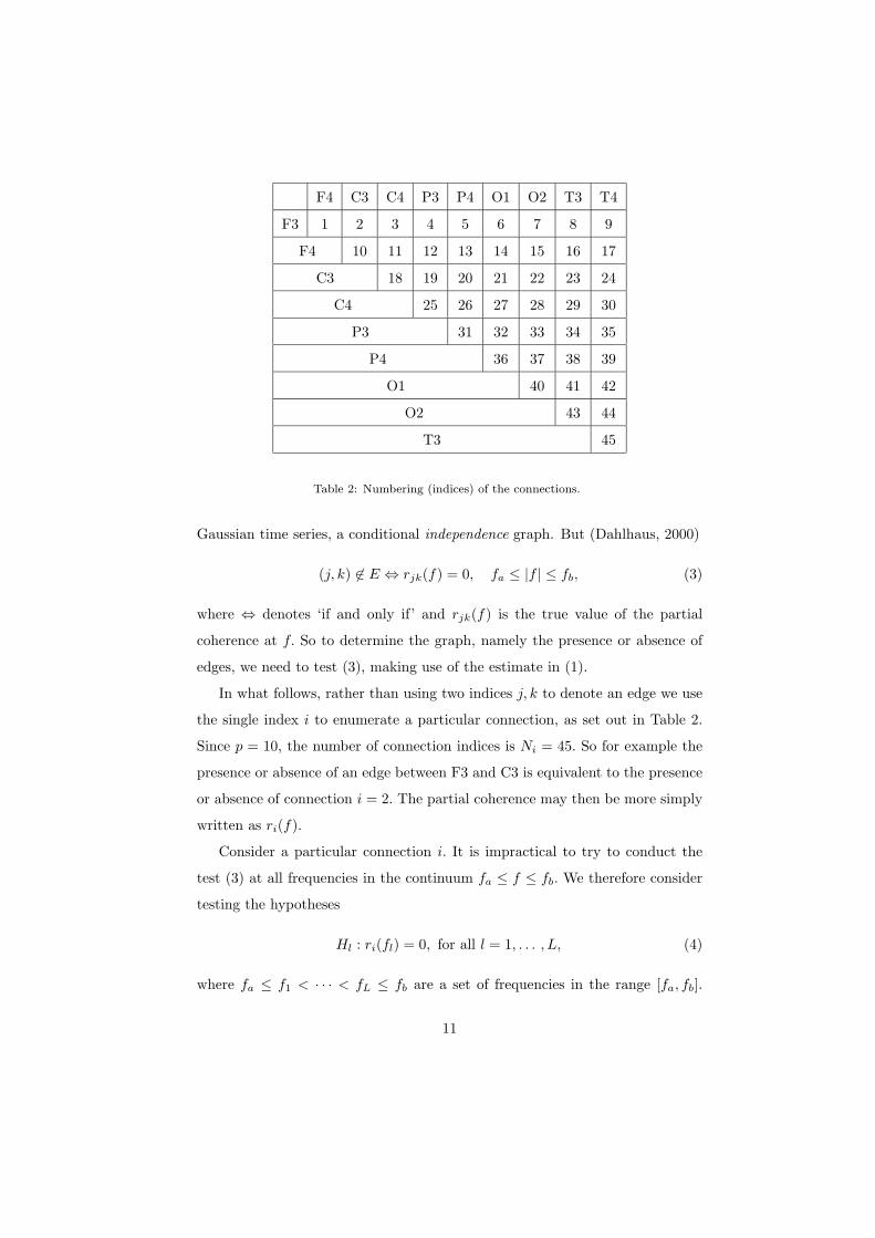
Table 2: Numbering (indices) of the connections.

Gaussian time series, a conditional independence graph. But (Dahlhaus, 2000)

(j, k) �∈ E ⇔ rjk(f) = 0, fa ≤ |f | ≤ fb, (3)

where ⇔ denotes ‘if and only if’ and rjk(f) is the true value of the partial

coherence at f. So to determine the graph, namely the presence or absence of

edges, we need to test (3), making use of the estimate in (1).

In what follows, rather than using two indices j, k to denote an edge we use

the single index i to enumerate a particular connection, as set out in Table 2.

Since p = 10, the number of connection indices is Ni = 45. So for example the

presence or absence of an edge between F3 and C3 is equivalent to the presence

or absence of connection i = 2. The partial coherence may then be more simply

written as ri(f).

Consider a particular connection i. It is impractical to try to conduct the

test (3) at all frequencies in the continuum fa ≤ f ≤ fb. We therefore consider

testing the hypotheses

Hl : ri(fl) = 0, for all l = 1, . . . , L, (4)

where fa ≤ f1 < · · · < fL ≤ fb are a set of frequencies in the range [fa, fb].

11

(By symmetry we need only consider positive frequencies.) This is a multiple

hypothesis testing problem. The test uses the known distribution of the raw

partial coherence ri(f) under the null hypothesis.

To carry out the multiple hypothesis testing we employ the stepdown method

combined with the Holm method for determining the set of critical values em-

ployed. The Holm procedure is suitable for multiple hypothesis testing when

the statistics being tested are correlated; this is the case here since the esti-

mation bandwidth is 5Hz, so the estimators {ri(fl), l = 1, . . . , L}, within the

delta band, are obviously correlated. Full details of the Holm procedure may be

found in Medkour et al. (2009); we required that the probability of one or more

false rejections should not exceed 0.05.

Graphical model selection

Measuring strengths of connections

We can determine the set of frequencies {fl′}, a subset of {fl}, consisting

of L′ elements (possibly zero), at which the null hypothesis Hl : ri(fl) = 0 is

rejected. While only one hypothesis need be rejected to indicate an edge between

{Xj,t} and {Xk,t}, or connection i, the knowledge of the set of frequencies where

rejection occurred gives us useful information of which we make use as follows.

In Medkour et al. (2009) we used L′/L, the ratio of the number of rejected

hypotheses to the total tested, to measure the strength of connection i. Here we

propose a weighted ratio measure where a rejected hypothesis at fl′ is weighted

by the corresponding debiassed estimated partial coherence ri(fl′) defined by

(2). There are three data-set groupings, P,N , C. For any grouping consider

combining results over individuals, indexed by a, a = 1, . . . , Na, and epochs,

indexed by b, b = 1, . . . , Nb. We therefore define the weighted ratio measure by

WRabi =

1L

L′∑l′=1

rabi (fl′). (5)

12

5 10 15 20 25 30 35 40 450

0.5

1

tota

l wgt

. rel

. str

engt

h

(a)

5 10 15 20 25 30 35 40 450

0.5

1

index

tota

l wgt

. rel

. str

engt

h

(b)

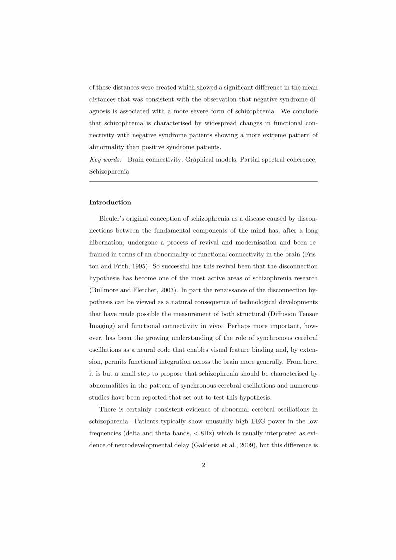
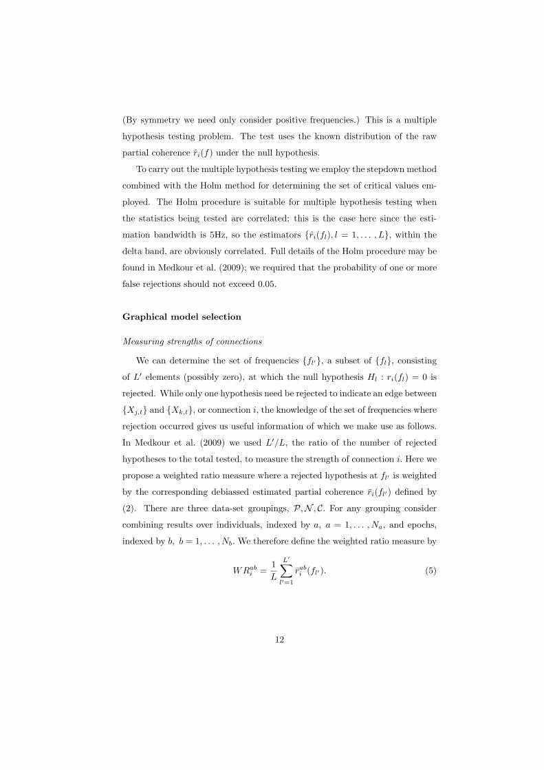
Figure 2: Total weighted relative strength, WRSi, against connection index i, for (a) positive-

syndrome patients, P, and (b) negative-syndrome patients, N .

Next we average WRabi over individuals (in the grouping) to obtain WR

b

i .

(This is our measure of the strength of the connection.) Now let PIbi denote the

proportion of individuals in the grouping which exhibit the connection i, i.e.,

(4) has been rejected. (This takes into account the incidence of the connection.)

Then we define the weighted relative strength by

WRSbi = WR

b

i · PIbi ,

and finally take the sum over the Nb epochs to obtain

WRSi =Nb∑b=1

WRSbi , (6)

which is the total weighted relative strength for connection i. The quantity

WRSi, i = 1, . . . , Ni, with Ni = 45, can be displayed as a vector. This is shown

for the groupings P and N in Fig. 2.

For total weighted relative strength we now show how we chose a threshold

T to enable us to discern the most significant connections.

13

0 0.05 0.1 0.150

10

20

30

40

50

60

v

(a)

0 0.05 0.1 0.150

5

10

15

20

25

30

35

v

(b)

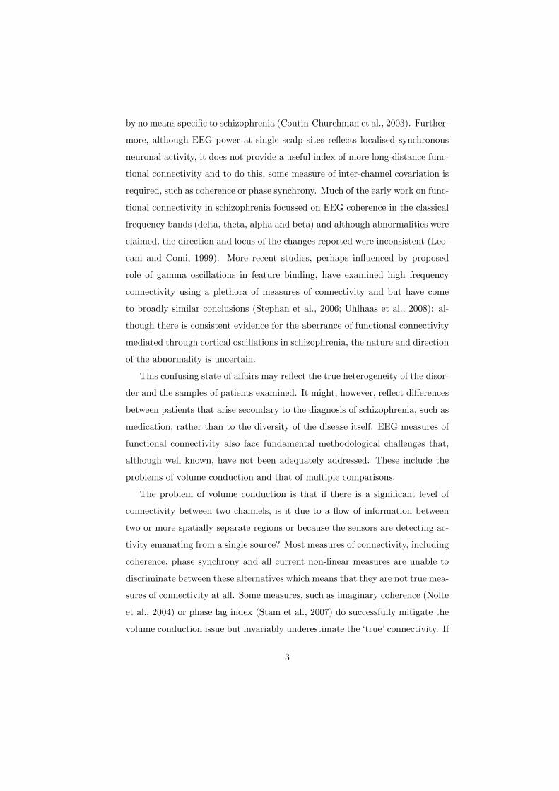
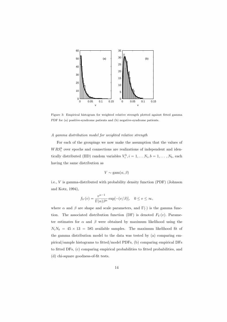
Figure 3: Empirical histogram for weighted relative strength plotted against fitted gamma

PDF for (a) positive-syndrome patients and (b) negative-syndrome patients.

A gamma distribution model for weighted relative strength

For each of the groupings we now make the assumption that the values of

WRSbi over epochs and connections are realizations of independent and iden-

tically distributed (IID) random variables V bi , i = 1, . . . Ni, b = 1, . . . , Nb, each

having the same distribution as

V ∼ gam(α, β)

i.e., V is gamma-distributed with probability density function (PDF) (Johnson

and Kotz, 1994),

fV (v) =vα−1

Γ(α)βαexp[−(v/β)], 0 ≤ v ≤ ∞,

where α and β are shape and scale parameters, and Γ(·) is the gamma func-

tion. The associated distribution function (DF) is denoted FV (v). Parame-

ter estimates for α and β were obtained by maximum likelihood using the

NiNb = 45 × 13 = 585 available samples. The maximum likelihood fit of

the gamma distribution model to the data was tested by (a) comparing em-

pirical/sample histograms to fitted/model PDFs, (b) comparing empirical DFs

to fitted DFs, (c) comparing empirical probabilities to fitted probabilities, and

(d) chi-square goodness-of-fit tests.

14

0 0.5 10

0.2

0.4

0.6

0.8

1

empi

rical

pro

babi

lity

theoretical probability

(a)

0 0.5 10

0.2

0.4

0.6

0.8

1

empi

rical

pro

babi

lity

theoretical probability

(b)

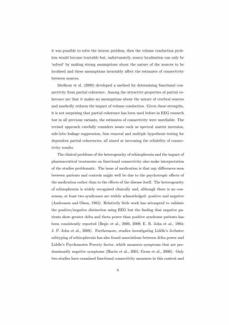
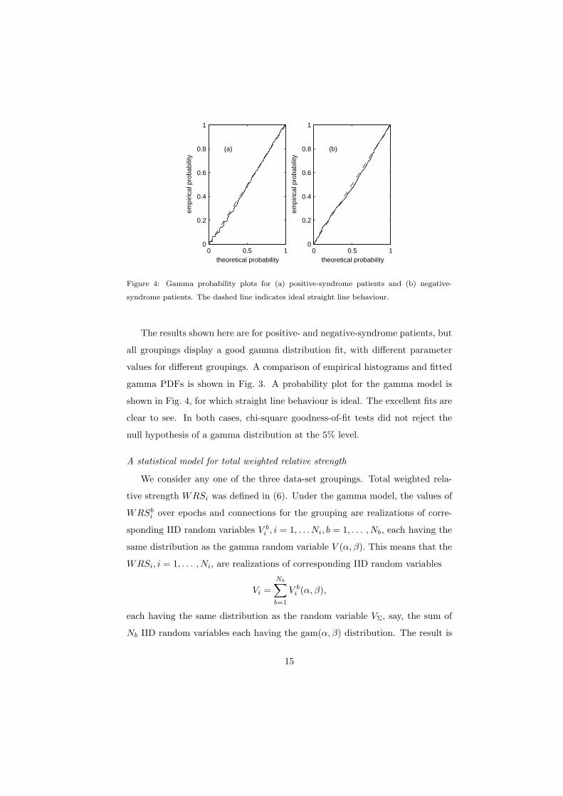
Figure 4: Gamma probability plots for (a) positive-syndrome patients and (b) negative-

syndrome patients. The dashed line indicates ideal straight line behaviour.

The results shown here are for positive- and negative-syndrome patients, but

all groupings display a good gamma distribution fit, with different parameter

values for different groupings. A comparison of empirical histograms and fitted

gamma PDFs is shown in Fig. 3. A probability plot for the gamma model is

shown in Fig. 4, for which straight line behaviour is ideal. The excellent fits are

clear to see. In both cases, chi-square goodness-of-fit tests did not reject the

null hypothesis of a gamma distribution at the 5% level.

A statistical model for total weighted relative strength

We consider any one of the three data-set groupings. Total weighted rela-

tive strength WRSi was defined in (6). Under the gamma model, the values of

WRSbi over epochs and connections for the grouping are realizations of corre-

sponding IID random variables V bi , i = 1, . . . Ni, b = 1, . . . , Nb, each having the

same distribution as the gamma random variable V (α, β). This means that the

WRSi, i = 1, . . . , Ni, are realizations of corresponding IID random variables

Vi =Nb∑b=1

V bi (α, β),

each having the same distribution as the random variable VΣ, say, the sum of

Nb IID random variables each having the gam(α, β) distribution. The result is

15

well-known,

VΣ ∼ gam(Nbα, β).

So the DF for VΣ is given by

FVΣ(v) =∫ v

0

yNbα−1

Γ(Nbα)βNbαexp[−(y/β)]dy

=∫ v/β

0

uNbα−1

Γ(Nbα)exp[−u]du

= Γ(v/β, Nbα),

where Γ(x, a) = [1/Γ(a)]∫ x

0e−tta−1dt is the incomplete gamma function.

Determining the graph

The connectivity graph for any of the data-set groupings is determined by

firstly specifying a threshold Tρ for total weighted relative strength as the quan-

tile of the distribution of VΣ corresponding to a chosen probability ρ found via

the DF, i.e.,

Tρ = F−1VΣ

(ρ). (7)

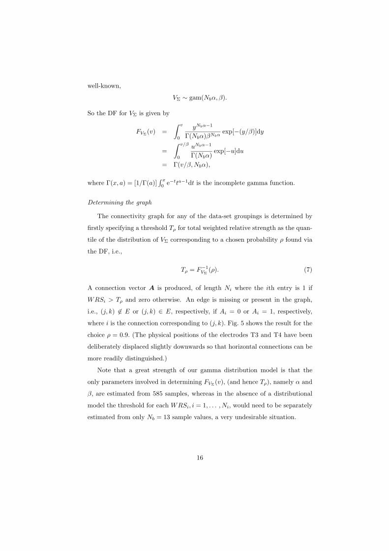
A connection vector A is produced, of length Ni where the ith entry is 1 if

WRSi > Tρ and zero otherwise. An edge is missing or present in the graph,

i.e., (j, k) �∈ E or (j, k) ∈ E, respectively, if Ai = 0 or Ai = 1, respectively,

where i is the connection corresponding to (j, k). Fig. 5 shows the result for the

choice ρ = 0.9. (The physical positions of the electrodes T3 and T4 have been

deliberately displaced slightly downwards so that horizontal connections can be

more readily distinguished.)

Note that a great strength of our gamma distribution model is that the

only parameters involved in determining FVΣ(v), (and hence Tρ), namely α and

β, are estimated from 585 samples, whereas in the absence of a distributional

model the threshold for each WRSi, i = 1, . . . , Ni, would need to be separately

estimated from only Nb = 13 sample values, a very undesirable situation.

16

F3 F4

C3 C4

P3 P4

O1 O2

T3 T4

F3 F4

C3 C4

P3 P4

O1 O2

T3 T4

F3 F4

C3 C4

P3 P4

O1 O2

T3 T4

F3 F4

C3 C4

P3 P4

O1 O2

T3 T4

F3 F4

C3 C4

P3 P4

O1 O2

T3 T4

F3 F4

C3 C4

P3 P4

O1 O2

T3 T4

F3 F4

C3 C4

P3 P4

O1 O2

T3 T4

F3 F4

C3 C4

P3 P4

O1 O2

T3 T4

F3 F4

C3 C4

P3 P4

O1 O2

T3 T4

F3 F4

C3 C4

P3 P4

O1 O2

T3 T4

F3 F4

C3 C4

P3 P4

O1 O2

T3 T4

F3 F4

C3 C4

P3 P4

O1 O2

T3 T4

F3 F4

C3 C4

P3 P4

O1 O2

T3 T4

F3 F4

C3 C4

P3 P4

O1 O2

T3 T4

F3 F4

C3 C4

P3 P4

O1 O2

T3 T4

F3 F4

C3 C4

P3 P4

O1 O2

T3 T4

F3 F4

C3 C4

P3 P4

O1 O2

T3 T4

F3 F4

C3 C4

P3 P4

O1 O2

T3 T4

F3 F4

C3 C4

P3 P4

O1 O2

T3 T4

F3 F4

C3 C4

P3 P4

O1 O2

T3 T4

F3 F4

C3 C4

P3 P4

O1 O2

T3 T4

F3 F4

C3 C4

P3 P4

O1 O2

T3 T4

F3 F4

C3 C4

P3 P4

O1 O2

T3 T4

F3 F4

C3 C4

P3 P4

O1 O2

T3 T4

F3 F4

C3 C4

P3 P4

O1 O2

T3 T4

F3 F4

C3 C4

P3 P4

O1 O2

T3 T4

F3 F4

C3 C4

P3 P4

O1 O2

T3 T4

F3 F4

C3 C4

P3 P4

O1 O2

T3 T4

F3 F4

C3 C4

P3 P4

O1 O2

T3 T4

F3 F4

C3 C4

P3 P4

O1 O2

T3 T4

Figure 5: Interactions for positive-syndrome patients, (top left), negative-syndrome patients,

(top right) and controls (bottom left), all for ρ = 0.9.

17

Summary of steps

For each grouping, P,N , C, the following steps are carried out.

• Step 1: The spectral matrix Sab(f), say, is estimated for individuals a =

1, . . . , Na and epochs b = 1, . . . , Nb.

• Step 2: The raw partial coherence, rabi (f), for all possible connections

i = 1, . . . , Ni set out in Table II is estimated for individuals a = 1, . . . , Na

and epochs b = 1, . . . , Nb. From this a debiassed version, rabi (f), is found

from (2). For each connection i the Holm stepdown procedure determines

the number L′ (possibly null) and set of frequencies {fl′} (possibly empty)

for which the hypothesis of null partial coherence is rejected.

• Step 3: The weighted ratios WRabi , defined in (5), are then computed and

averaged over individuals a = 1, . . . , Na in the grouping to give WRb

i .

• Step 4: The proportion of individuals in the grouping which exhibit con-

nection i, namely PIbi is found next. Then the weighted relative strength

is found from WRSbi = WR

b

i · PIbi .

• Step 5: The WRSbi values are well-fitted by a gamma distribution with

parameters α and β estimated by maximum likelihood, whence WRSi =∑Nb

b=1 WRSbi , i = 1, . . . , Ni, is a sample from a gamma distribution with

parameters Nbα and β. WRSi is the total weighted relative strength for

connection i.

• Step 6: For a chosen probability ρ a threshold Tρ for total weighted relative

strength is determined as the corresponding quantile of the gam(Nbα, β)

distribution. For the grouping under consideration, a connection vector

A is produced, of length Ni where the ith entry is 1 if WRSi > Tρ and

zero otherwise.

• Step 7: The graph is constructed using the rule that an edge is present in

the graph, i.e., (j, k) ∈ E, if Ai = 1. The graph depends on the choice of

ρ.

18

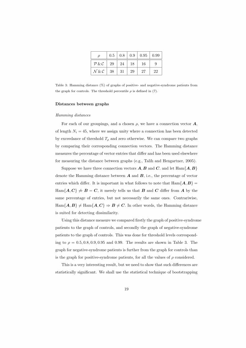
ρ 0.5 0.8 0.9 0.95 0.99

P & C 29 24 18 16 9

N & C 38 31 29 27 22

Table 3: Hamming distance (%) of graphs of positive- and negative-syndrome patients from

the graph for controls. The threshold percentile ρ is defined in (7).

Distances between graphs

Hamming distances

For each of our groupings, and a chosen ρ, we have a connection vector A,

of length Ni = 45, where we assign unity where a connection has been detected

by exceedance of threshold Tρ and zero otherwise. We can compare two graphs

by comparing their corresponding connection vectors. The Hamming distance

measures the percentage of vector entries that differ and has been used elsewhere

for measuring the distance between graphs (e.g., Talih and Hengartner, 2005).

Suppose we have three connection vectors A,B and C. and let Ham{A,B}denote the Hamming distance between A and B, i.e., the percentage of vector

entries which differ. It is important in what follows to note that Ham{A,B} =

Ham{A,C} �⇒ B = C, it merely tells us that B and C differ from A by the

same percentage of entries, but not necessarily the same ones. Contrariwise,

Ham{A,B} �= Ham{A,C} ⇒ B �= C. In other words, the Hamming distance

is suited for detecting dissimilarity.

Using this distance measure we compared firstly the graph of positive-syndrome

patients to the graph of controls, and secondly the graph of negative-syndrome

patients to the graph of controls. This was done for threshold levels correspond-

ing to ρ = 0.5, 0.8, 0.9, 0.95 and 0.99. The results are shown in Table 3. The

graph for negative-syndrome patients is further from the graph for controls than

is the graph for positive-syndrome patients, for all the values of ρ considered.

This is a very interesting result, but we need to show that such differences are

statistically significant. We shall use the statistical technique of bootstrapping

19

to investigate this.

Bootstrapping and t test

Given our assumption that the multi-channel correlation structure is invari-

ant across epochs, the epochs can be treated as exchangeable in our application

in the same sense that elements of a random sample are treated as such in the

standard bootstrapping scheme (Efron and Tibshirani, 1993).

For each grouping, and given individual a and connection i, let us denote

the indices of the epochs used in our scheme up to now by b = b1, . . . , bNb,

where bj = j. With bootstrapping we draw a random sample of size Nb from

b1, . . . , bNb, with replacement. We denote these indices by b∗ = b∗1, . . . , b∗Nb

, a

list which may contain some integers in the range 1, . . . , Nb more than once,

and others not at all. Analysis steps 3 to 7 are modified as follows (unchanged

details are excluded):

• Step 3∗: We draw the sample b∗ = b∗1, . . . , b∗Nb. The weighted ratios

WRab∗i , b∗ = b∗1, . . . , b∗Nb

, are averaged over individuals a = 1, . . . , Na

in the grouping to give WRb∗

i .

• Step 4∗: The proportion of individuals in the grouping which exhibit con-

nection i, namely PIb∗i is found next. Then the weighted relative strength

is found from WRSb∗i = WR

b∗

i · PIb∗i , for b∗ = b∗1, . . . , b∗Nb

, i = 1, . . . , Ni.

• Step 5∗: WRSi =∑

b∗ WRSb∗i , i = 1, . . . , Ni, is a sample from a gamma

distribution with parameters Nbα and β.

• Step 6∗: For the grouping under consideration, a connection vector A∗1 is

produced, of length Ni where the ith entry is 1 if WRSi > Tρ and zero

otherwise.

• Step 7∗: The graph is constructed using the rule that connection i is

present in the graph, i.e., (j, k) ∈ E, if A∗1,i = 1.

Steps 3∗ to 7∗ are repeated a large number Nr = 5000 times to obtain connection

vectors AP∗1 , . . . ,AP∗

Nrfor patients diagnosed with positive syndrome, and then

20

0.2 0.4 0.60

2

4

6

8

10

distance

0 0.2 0.40

2

4

6

8

10

distance

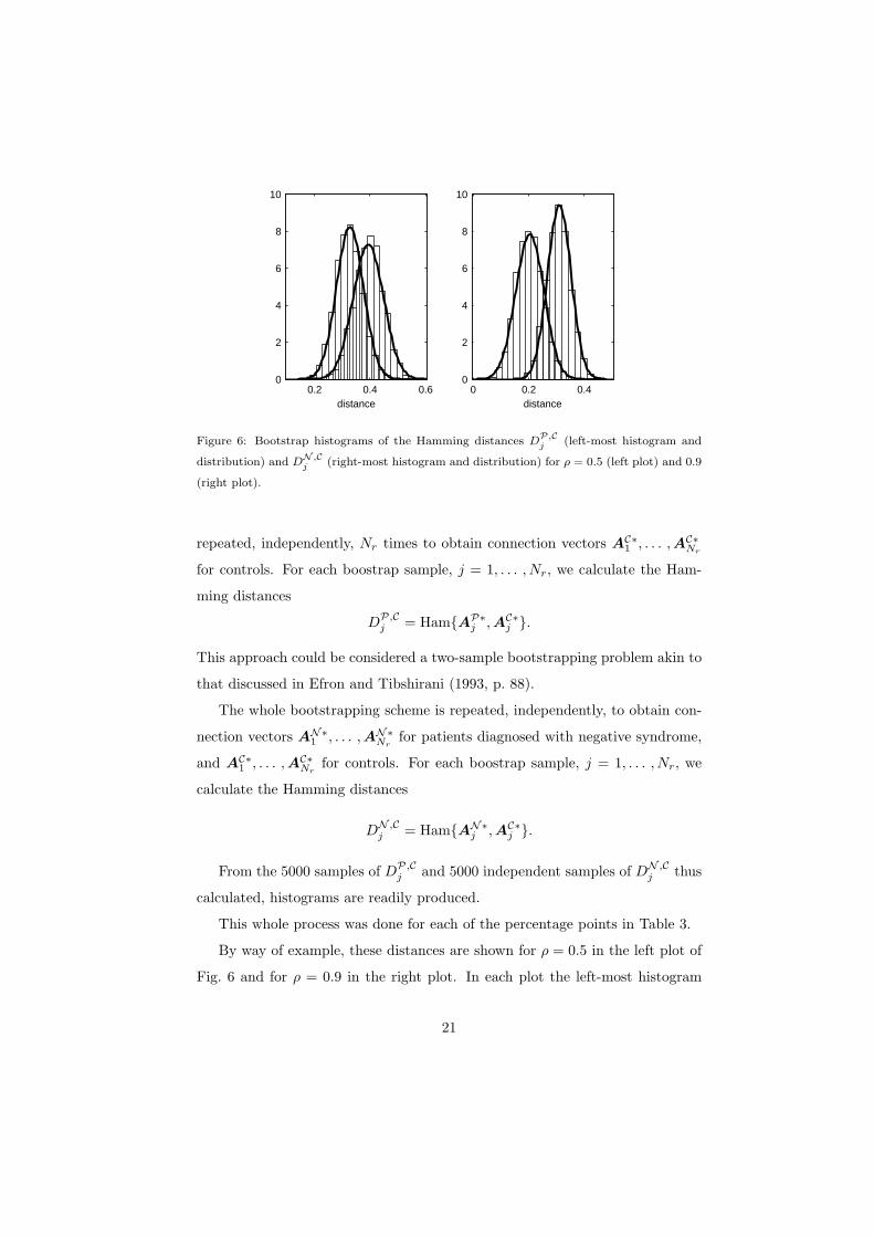
Figure 6: Bootstrap histograms of the Hamming distances DP,C

j (left-most histogram and

distribution) and DN ,Cj (right-most histogram and distribution) for ρ = 0.5 (left plot) and 0.9

(right plot).

repeated, independently, Nr times to obtain connection vectors AC∗1 , . . . ,AC∗

Nr

for controls. For each boostrap sample, j = 1, . . . , Nr, we calculate the Ham-

ming distances

DP,Cj = Ham{AP∗

j ,AC∗j }.

This approach could be considered a two-sample bootstrapping problem akin to

that discussed in Efron and Tibshirani (1993, p. 88).

The whole bootstrapping scheme is repeated, independently, to obtain con-

nection vectors AN∗1 , . . . ,AN∗

Nrfor patients diagnosed with negative syndrome,

and AC∗1 , . . . ,AC∗

Nrfor controls. For each boostrap sample, j = 1, . . . , Nr, we

calculate the Hamming distances

DN ,Cj = Ham{AN∗

j ,AC∗j }.

From the 5000 samples of DP,Cj and 5000 independent samples of DN ,C

j thus

calculated, histograms are readily produced.

This whole process was done for each of the percentage points in Table 3.

By way of example, these distances are shown for ρ = 0.5 in the left plot of

Fig. 6 and for ρ = 0.9 in the right plot. In each plot the left-most histogram

21

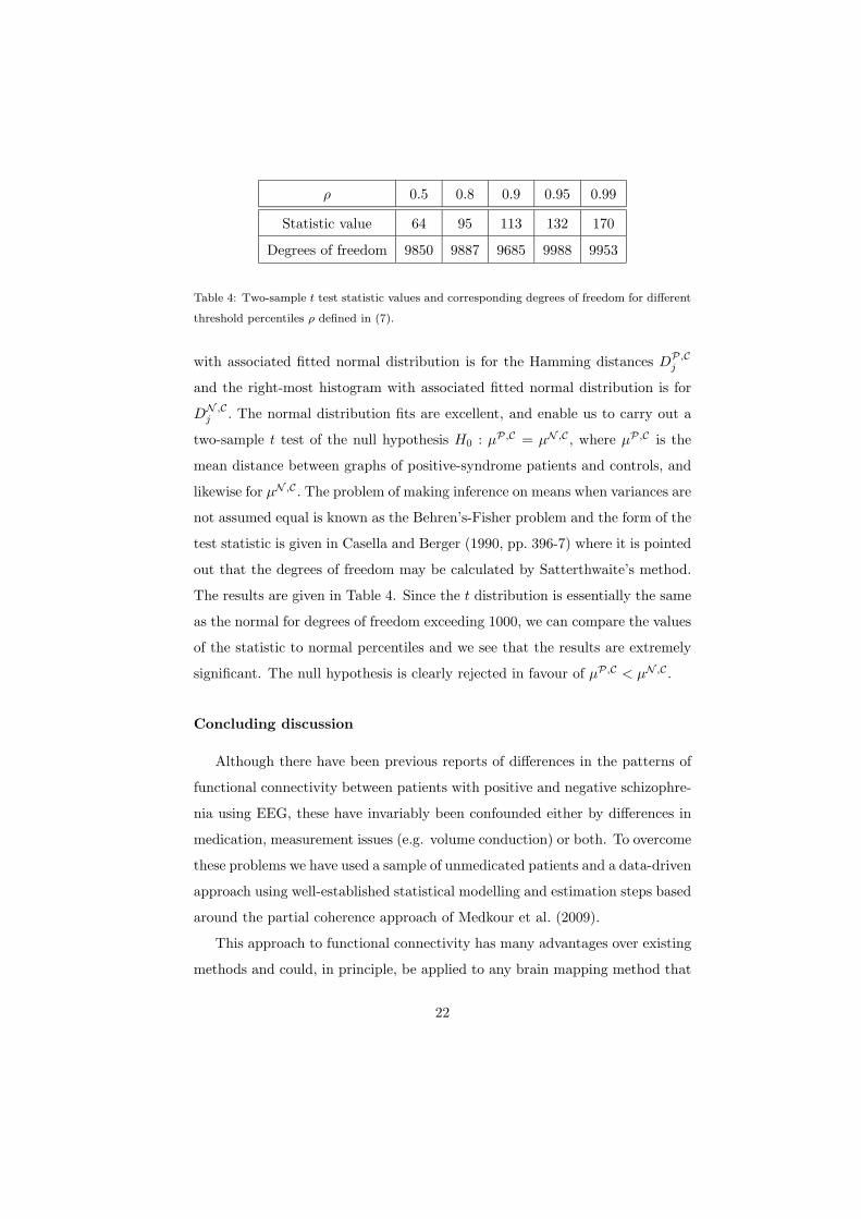
ρ 0.5 0.8 0.9 0.95 0.99

Statistic value 64 95 113 132 170

Degrees of freedom 9850 9887 9685 9988 9953

Table 4: Two-sample t test statistic values and corresponding degrees of freedom for different

threshold percentiles ρ defined in (7).

with associated fitted normal distribution is for the Hamming distances DP,Cj

and the right-most histogram with associated fitted normal distribution is for

DN ,Cj . The normal distribution fits are excellent, and enable us to carry out a

two-sample t test of the null hypothesis H0 : µP,C = µN ,C , where µP,C is the

mean distance between graphs of positive-syndrome patients and controls, and

likewise for µN ,C . The problem of making inference on means when variances are

not assumed equal is known as the Behren’s-Fisher problem and the form of the

test statistic is given in Casella and Berger (1990, pp. 396-7) where it is pointed

out that the degrees of freedom may be calculated by Satterthwaite’s method.

The results are given in Table 4. Since the t distribution is essentially the same

as the normal for degrees of freedom exceeding 1000, we can compare the values

of the statistic to normal percentiles and we see that the results are extremely

significant. The null hypothesis is clearly rejected in favour of µP,C < µN ,C .

Concluding discussion

Although there have been previous reports of differences in the patterns of

functional connectivity between patients with positive and negative schizophre-

nia using EEG, these have invariably been confounded either by differences in

medication, measurement issues (e.g. volume conduction) or both. To overcome

these problems we have used a sample of unmedicated patients and a data-driven

approach using well-established statistical modelling and estimation steps based

around the partial coherence approach of Medkour et al. (2009).

This approach to functional connectivity has many advantages over existing

methods and could, in principle, be applied to any brain mapping method that

22

generates time-series data. The greatest benefits, however, are likely to be seen

in EEG or MEG studies. Currently, the method is limited to cases of graphs

with relatively few nodes: the non-singularity of estimated spectral matrices is

a key requirement, and the current authors are considering ways to deal with

this problem for dense array EEG/MEG data in sensor space. Prior reduction

of the dimensionality of the data by, for example, source localisation, would also

be a valid approach.

With the presented methodological advances, we have been able to show for

the first time that there are reliable differences in the patterns of functional

connectivity between patients with positive and negative schizophrenia. Our

results indicate that the brain connectivity graphs for patients diagnosed with

negative syndrome are on average further from the graphs of controls than are

the brain connectivity graphs for patients diagnosed with positive syndrome.

This is consistent with the idea that the negative syndrome is a more severe

form of schizophrenia with symptoms entailing greater disability and poorer

prognosis (Fenton and McGlashan, 1991).

These findings are not, however, consistent with the concept of schizophrenia

as a simple disconnection syndrome. For neither syndrome was it the case that

the patients’ graphs were simply diminished versions of the controls’. Rather,

our findings support the more general notion of a ‘dysconnection’ syndrome

(Stephan et al., 2006) whereby schizophrenia is characterised not only by the

absence of functional connectivity but also by the presence of aberrant con-

nections. Why might this be? Firstly, the measure of connectivity we use is

functional, not structural. Patients might have a normal brain structure but

be using their brain in a non-standard way. For example, in recovery from

brain injury, some improvement results from patients solving a problem by us-

ing a different strategy (i.e., one that does not require the damaged part of the

brain). Something comparable might be going on here, namely patients using

different cognitive strategies to controls. Secondly, in normal development, the

brain starts with far more neurones and synaptic connections than it needs and

around the time of adolesence, there is massive synaptic pruning leading to a loss

23

of many neurones. Pruning is based on the synaptic strength which is derived

from how many times each synapse has been activated: more activation, more

synaptic strength. In schizophrenia, abnormal development leads to atypical

development of synaptic strengths which is latent in childhood because of the

massive redundancy of neural tissue. However, in schizophrenia, because of the

abnormal synaptic strengths, when the pruning process starts, some connections

that are useful are lost, and others that are aberrant will be kept.

Given the well-known spatial limitations of EEG, the present results have

little to say about the localisation of the brain regions that gave rise to the

dysconnections observed. However connections were seen in the frontal, tempo-

ral, parietal and occipital regions and in both the left and right hemispheres.

Furthermore, multiple long-range connections were found both between lobes

and between hemispheres. The implication of this must be that schizophrenia,

and its major subtypes, are characterised by widespread abnormalities in the

pattern of connectivity.

Acknowledgements

The work of TM, ATW and APB was supported by the Engineering and

Physical Science Research Council (UK) and the Medical Research Council (UK)

and that of VBS by grants from the Russian Foundation for Humanities (No.

09-06-00-459a) and from the BIAL Foundation (No. 20/02). Helpful suggestions

by the referees were much appreciated.

References

Andreasen, N. C., Olsen, S. A., 1982. Negative v positive schizophrenia: Defi-

nition and validation. Archives of General Psychiatry 39, 789-794.

Andreasen, N. C., 1983. The Scale for the Assessment of Negative Symptoms

(SANS). The University of Iowa, Iowa City, IA.

24

Andreasen, N. C., 1984. The Scale for the Assessment of Positive Symptoms

(SAPS). The University of Iowa, Iowa City, IA.

Begic, D., Hotujac, L., Jokic-Begic, N., 2000. Quantitative EEG in ‘positive’

and ‘negative’ schizophrenia. Acta Psychiatrica Scandinavica, 101, 307-311.

Begic, D., Mahnik-Milos, M., Grubisin, J., 2009. EEG characteristics in depres-

sion, ‘negative’ and ‘positive’ and schizophrenia. Psychiatria Danubina 21,

579-584.

Benignus, V. A., 1969. Estimation of the coherence spectrum and its confidence

interval using the fast Fourier transform. IEEE Trans. Audio and Electroa-

coustics 17, 145-150.

Bullmore, E., Fletcher, P., 2003. The eye’s mind: brain mapping and psychiatry.

British J. Psychiatry 182, 381-384.

Casella, G., Berger, R. L., 1990. Statistical Inference. Wadsworth, Inc., Belmont

CA.

Coutin-Churchman, P., Anez, Y., Uzcategui, M., Alvarez, L., Vergara, F.,

Mendez, L. and Fleitas, R., 2003. Quantitative spectral analysis of EEG in

psychiatry revisited: drawing signs out of numbers in a clinical setting. Clin.

Neurophysiology 114, 2294-2306.

Dahlhaus, R., 2000. Graphical interaction models for multivariate time series.

Metrika 51, 157-72.

Dahlhaus, R., Eichler, M., Sandkuhler, J., 1997. Identification of synaptic con-

nections in neural ensembles by graphical models. J. Neurosci. Meth. 77, 93-

107.

Dawson, G., Fischer, K.W., 1994. Human Behavior and the Developing Brain.

The Guilford Press.

Efron, B., Tibshirani, R. J., 1993. An Introduction to the Bootstrap. Chapman

& Hall/CRC.

25

Fenton, W. S., McGlashan, T.H., 1991. Natural history of schizophrenia sub-

types II: positive and negative symptoms and long-term course. Arch. Gen.

Psychiatry. 48, 978-986.

Fiecas, M., Ombao, H., Linkletter, C., Thompson, W., Sanes, J., 2010. Func-

tional connectivity: shrinkage estimation and randomization test. NeuroIm-

age 49, 3005-3014.

Friston K. J., Frith, C. D., 1995. Schizophrenia: a disconnection syndrome?

Clin. Neurosci. 3, 89-97.

Galderisi, S., Mucci, A., Volpe, U., Boutros, N., 2009. Evidence-based medicine

and electrophysiology in schizophrenia. Clin. EEG Neurosci. 40, 62-77.

Gross, A., Joutsiniemi, S-L., Rimon, R., Appelberg, B., 2006. Correlation

of symptom clusters of schizophrenia with absolute powers of main fre-

quency bands in quantitative EEG. Behavioral and Brain Functions 2, 23.

doi:10.1186/1744-9081-2-23.

Harris, A. W. F., Bahramali, H., Slewa-Younan, S., Gordon, E., Williams, L.,

Li W. M., 2001. The topography of quantified electroencephalography in three

syndromes of schizophrenia. Int. J. Neurosci. 107, 265-278.

John, E. R., Prichep, L. S., Alper, K. R., Mas, F. G., Cancro, R., Easton, P.,

Sverdlov, L., 1994. Quantitative electrophysiological characteristics and sub-

typing of schizophrenia. Biol. Psychiatry 36, 801-826.

John, J.P., Rangaswamy, M., Thennarasu, K., Khanna, S., Nagaraj, R. B.,

Mukundan, C.R., Pradhan, N., 2009. EEG power spectra differentiate pos-

itive and negative subgroups in neuroleptic-naive schizophrenia patients. J.

Neuropsychiatry Clin. Neurosci. 21, 160-172.

Johnson, N. L., Kotz, S., Balakrishnan, N., 1994. Continuous Univariate Distri-

butions, 2nd ed., vol. 1: Models and Applications. John Wiley & Sons, Inc.,

New York.

26

Lee, K-H., Williams, L. M., Breakspear, M., Gordon, E., 2003. Synchronous

gamma activity: A review and contribution to an integrative neuroscience

model of schizophrenia. Brain Res. Rev. 41, 57-78.

Leocani, L., Comi G., 1999. EEG coherence in pathological conditions. J. Clin.

Neurophysiol. 16, 548-555.

Medkour, T., Walden, A. T., Burgess, A., 2009. Graphical modelling for brain

connectivity via partial coherence. J. Neurosci. Meth. 180, 374-383.

Nolte, G., Ou, B., Wheaton, L., Mari, Z., Vorbach, S., Hallett, M., 2004. Iden-

tifying true brain interaction from EEG data using the imaginary part of

coherency. Clin. Neurophysiol. 115, 2292-2307.

Percival, D. B., Walden, A. T., 1993. Spectral Analysis for Physical Applica-

tions. Cambridge University Press, Cambridge UK.

Salvador, R., Suckling, J., Schwarzbauer, C., Bullmore, E., 2005. Undirected

graphs of frequency-dependent functional connectivity in whole brain net-

works. Phil. Trans. Roy. Soc. Lond., Ser. B, 360, 937-46.

Stam, C. J., Nolte, G., Daffertshofer, A., 2007. Phase lag index: assessment of

functional connectivity from multichannel EEG and MEG with diminished

bias from common sources. Hum. Brain Mapp. 28, 1178-1193.

Stephan, K. E., Baldeweg, T., Friston, K. J., 2006. Synaptic plasticity and

dysconnection in schizophrenia. Biological Psychiatry 59, 929-939.

Strelets, V. B., Novototsky-Vlasov, V. Y., Golikova, J. V., 2002. Cortical con-

nectivity in high frequency beta-rhythm in schizophrenics with positive and

negative symptoms. Int. J. Psychophysiol. 44, 101-115.

Talih, M., Hengartner, N., 2005. Structural learning with time-varying compo-

nents: tracking the cross-section of financial time series. J. Roy. Statist. Soc.

Ser. B, 67, 321-341.

27

Uhlhaas, P.J., Haenschel, C., Nikolic, D., Singer, W., 2008. The role of oscilla-

tions and synchrony in cortical networks and their putative relevance for the

pathophysiology of schizophrenia. Schizophrenia Bull. 34, 927-943.

Walden, A. T., McCoy, E. J., Percival, D. B., 1995. The effective bandwidth of

a multitaper spectral estimator. Biometrika 82, 201-14.

28