Boyd’s conjecture for a family of genus 2 curves
73
Boyd’s conjecture for a family of genus 2 curves Johan Bosman May 2004
Transcript of Boyd’s conjecture for a family of genus 2 curves
Boyd’s conjecture for a family of genus 2 curves
Johan Bosman
May 2004


Contents
1 Introduction 1
2 Some elementary properties of the Mahler measure 42.1 Polynomials of the form A(x)y2 +B(x)y + C(x) . . . . . . . . . . . . . . . . . . . 6
3 Elliptic curves 73.1 Elliptic curves over Q . . . . . . . . . . . . . . . . . . . . . . . . . . . . . . . . . . 83.2 Elliptic curves over C . . . . . . . . . . . . . . . . . . . . . . . . . . . . . . . . . . 83.3 Divisors on an elliptic curve . . . . . . . . . . . . . . . . . . . . . . . . . . . . . . . 10
4 Steinberg symbols and K2 11
5 Dilogarithms and Eisenstein-Kronecker-Lerch series 145.1 The dilogarithm . . . . . . . . . . . . . . . . . . . . . . . . . . . . . . . . . . . . . 145.2 The elliptic dilogarithm . . . . . . . . . . . . . . . . . . . . . . . . . . . . . . . . . 155.3 Eisenstein-Kronecker-Lerch series . . . . . . . . . . . . . . . . . . . . . . . . . . . . 15
6 Regulators 186.1 Dilogarithm identities . . . . . . . . . . . . . . . . . . . . . . . . . . . . . . . . . . 24
7 Elliptic curves with complex multiplication 267.1 The curve y2 = x3 + 1 . . . . . . . . . . . . . . . . . . . . . . . . . . . . . . . . . . 31
8 Hyperelliptic curves 358.1 Homology of hyperelliptic curves . . . . . . . . . . . . . . . . . . . . . . . . . . . . 37
9 Reciprocal genus 2 curves 409.1 Homology . . . . . . . . . . . . . . . . . . . . . . . . . . . . . . . . . . . . . . . . . 41
10 The family Pk(x, y) = y2 + (x4 + kx3 + 2kx2 + kx+ 1)y + x4 4310.1 Construction of closed paths γk on C ′k . . . . . . . . . . . . . . . . . . . . . . . . . 4410.2 Degenerate cases . . . . . . . . . . . . . . . . . . . . . . . . . . . . . . . . . . . . . 51
10.2.1 The case k = 8 . . . . . . . . . . . . . . . . . . . . . . . . . . . . . . . . . . 5210.2.2 The case k = −1 . . . . . . . . . . . . . . . . . . . . . . . . . . . . . . . . . 53
10.3 Homology of Ck . . . . . . . . . . . . . . . . . . . . . . . . . . . . . . . . . . . . . . 5810.4 Pushing forward rC(f, g) . . . . . . . . . . . . . . . . . . . . . . . . . . . . . . . . . 6110.5 The case k = 2 . . . . . . . . . . . . . . . . . . . . . . . . . . . . . . . . . . . . . . 63
11 Conclusion 66
iii


1 Introduction
Let P be a nonzero laurent polynomial in n variables with coefficients in C (this means that P isan element of C[x1, . . . , xn, x
−11 , . . . , x−1
n ]). Then we define its (logarithmic) Mahler measure m(P )as follows:
m(P ) :=∫ 1
0
· · ·∫ 1
0
log |P (e2πit1 , . . . , e2πitn)|dt1 · · · dtn. (1)
Because all the singularities of the integrand are logarithmic, this integral converges and is well-defined. In general, it is very hard to compute the Mahler measure of a polynomial, there are onlyvery few cases for which explicit formulas are known. In this thesis we will be concerned aboutpolynomials in 2 variables with integer coefficients.
This Mahler measure looks like a strange integral but in fact it is a generalization of the heigthfunction in algebraic number theory: if α is an algebraic number and P is its minimal polynomialover Z, then the number m(P )/deg(P ) is known as the height of α and is denoted by h(α), whichcan also be defined as
h(α) =1
[K : Q]
∑v∈val(K)
max(0,[Kv : Qv|Q
]log |α|v
),
where one can take for K an arbitrary number field containing α.
Often it seems that we can relate the Mahler measure of a polynomial to the special value of anL-series. Let’s first look at the L-series of a dirichlet character χ of Z. It is defined as follows:
L(χ, s) =∞∑n=1
χ(n)n−s =∏
p prime
11− χ(p)p−s
. (2)
This L-series converges absolutely and uniformly on compacts sets for <s > 1 but it has analyticcontinuation to the entire complex plane together with a functional equation relating L(χ, s) andL(χ, 1− s).
Let m be a positive integer congruent to 0 or 3 modulo 4. Suppose that χ is an odd real-valuedDirichlet character, with a given minimal period m (a charachter is called odd if χ(−1) = −1).It’s known that only one such nontrivial χ exists, namely the Jacobi-symbol χ(n) =
(−mn
), see for
example [26] (even if you don’t want to check this, it’s a good book to read). Let’s denote thischaracter by χ−m. There is a functional equation for L(χ, s) from which it follows that
L′(χ−m,−1) =m√m
4πL(χ−m, 2), (3)
where L′(χ, s) simply denotes ddsL(χ, s).
In [4] the authors show how the Mahler measure of a polynomial P can be expressed in termsof the so called dilogarithm function (for its definition, look at section 5) if P is of the formA(x)y + B(x). In some cases this dilogarithm can be expressed in terms of L(χ, 2) and thus interms of L′(χ,−1). They prove, among many other examples, that
m(y + x+ 1) = L′(χ−3,−1) and m(y + x2 + x+ 1) =23L′(χ−4,−1).
Another example of an L-series which seems to occur in the computation of Mahler measures isthat of an elliptic curve: if E is an elliptic curve over Q, defined by a minimal equation with
1

coeffincients in Z then we can define the L-series of E as follows:
L(E, s) =∏
p|∆(E)
11− app−s
·∏p-∆E
11− app−s + p1−2s
,
where p runs through all prime numbers and ap = p + 1 − #E(Fp). This product converges for<s > 3
2 . There is also a functional equation relating L(E, s) and L(E, 2− s). In fact this followsfrom the celebrated theorem of Wiles, Taylor and others that every elliptic curve is modular,implying Fermat’s Last Theorem.
The first conjectural identity involving an L-series of an elliptic curve was found by Deninger, whogave a cohomological interpretation of m(P ), see [7]. He found this way the following formula tohold numerically:
m(x+1x
+ 1 + y +1y) = L′(E, 0),
where E is the elliptic curve defined by the polynomial x + 1x + 1 + y + 1
y of which the Mahlermeasure is taken. Inspired by this example, in [4], David Boyd gives several lists of polynomialsP of which he conjectures the following:
m(P ) = rL′(E, 0),
where r ∈ Q and E is an elliptic curve. In most cases, the elliptic curve E is isomorphic to (thejacobian variety of) the zero set of P . For these cases, Fernando Rodriguez Villegas gives aninteresting method to tackle the problem (see [17]). But Boyd also gives some families of P whichdefine curves of genus 2. In this thesis we will try to tackle the problem for that case.
The precise family of polynomials that we will study is
Pk(x, y) = y2 + (x4 + kx3 + 2kx2 + kx+ 1)y + x4.
Although the zero set of this polynomial is generically a curve of genus 2, it seems that m(Pk) is arational multiple of L′(E, 0) for k ∈ Z≤4 − −1 with E a certain elliptic curve that is a factor ofthe jacobian of the genus 2 curve. Also it appears that m(Pk) is a rational multiple of L′(χ,−1)for k ∈ −1, 8 with χ a certain real-valued Dirichlet character. In this thesis we will prove thefollowing:
Theorem 1 Let Pk(x, y) = y2 + (x4 + kx3 + 2kx2 + kx+ 1)y + x4. Then
m(P2) = L′(E, 0) with E : y2 = x3 + 1,m(P−1) = 2L′(χ−3,−1),m(P8) = 4L′(χ−4,−1).
These three identities can be found back in propositions 8, 7 and 6 respectively.
Although I succeeded in proving these identities, I still don’t understand why such identities mustbe valid. These proofs give a deduction which one can verify step-by-step but they seem to existcoincidentally. It is not at all clear how the arithmetic structure of the polynomials is related tothe arithmetic structure of the L-series. We will rewrite the integral to so-called dilogarithm sumsand these we will rewrite in terms of L-series. It is an open problem whether this is always possible.In the elliptic curve case it is not clear at all how to prove a relation between the dilogarithm sumsand the L-series, except for a few instances.
It is based on the Bloch-Beilinson conjecture. To be able to understand this conjecture, one firsthas to read sections 4 and 6 first. Let C be a complete nonsingular curve over Q and let g be its
2
genus. Let KT2 (C) be the subgroup of K2(Q(C)) consisting of those elements for which the tame
symbol vanishes at every Q-rational point of C. Furthermore, let H1(C(C),Z)− be the subgroupof H1(C(C),Z) consisting of the homology classes that are anti-invariant under the action ofcomplex conjugation. It is easy to see that this is a free abelian group of rank g. Define thefollowing pairing:
〈·, ·〉 : H1(C(C),Z)− ×KT2 (C)/ torsion → R : 〈γ, α〉 7→ 1
2π
∫γ
η(α).
The original conjecture of Beilinson states the following:
Conjecture 1 The abelian group KT2 (C)/ torsion is free of rank g and the given pairing is non-
degenerate. If we choose bases for the groups KT2 (C)/ torsion and H1(C(C),Z)− then the deter-
minant of the pairing is a rational multiple of π−2gL(C, 2), where L(C, s) denotes the L-series ofC.
However, this conjecture turned out to be incorrect. The rank of KT2 (C)/ torsion can be higher
than 1 in the case g = 1, as is pointed out in [3]. The computer experiments done in that articleinspired Bloch to do a reformulation of the Beilinson conjecture. Instead of looking solely at thecurve C over Q, we now take a model C of C over Z, which is regular and proper. Then not onlyfor each point P of C = CQ but also for each prime number p and each irreducible component D ofthe fiber Cp, we have a tame symbol K2(Q(C)) → Fp(D)∗. We define KT
2 (C) to be the subgroupof K2(Q(C)) consisting of those elements for which all the tame symbols, including the new ones,vanish. The reformulated conjecture is now
Conjecture 2 The abelian group KT2 (C)/ torsion is free of rank g and the given pairing is nonde-
generate. If we choose bases for the groups KT2 (C)/ torsion and H1(C(C),Z)− then the determinant
of the pairing is a rational multiple of π−2gL(C, 2).
For another experimental verification of this conjecture, see [9]. To my knowledge, the conjectureis at present far from solved. The rank of KT
2 (C)/ torsion hasn’t been proven to be finite. Whathas been proven is that in the case that E is an elliptic curve with complex multiplication thereexists an element of KT
2 (E)/ torsion, representable as a sum of elements f, g whose divisors arefully supported on torsion points, for which the pairing (with any element of H1(C(C),Z)− ofcourse) gives a rational multiple of π−2L(E, 2), see [2], [8] and also section 7 of this thesis. Also,for several modular curves C, the L-series part of the conjecture follows from the rank part, see[19].
3

2 Some elementary properties of the Mahler measure
Let n be a positive integer. Then we define the n-torus Tn as follows:
Tn := (z1, . . . , zn) ∈ Cn : |z1| = |z2| = · · · = |zn| = 1.
We have a parametrization [0, 1[n→ Tn by
(θ1, . . . , θn) 7→ (e2πiθ1 , . . . , e2πiθn).
If we make a change of variables using this parametrization, then (1) goes over into
m(P ) =1
(2πi)n
∫· · ·∫Tn
log |P (x1, . . . , xn)|dx1
x1· · · dxn
xn.
If n < m, then C[x±11 , . . . , x±1
n ] ⊂ C[x±11 , . . . , x±1
m ], so if P is a polynomial in n variables we cancompute its mahler measure as an n-fold integral, but also as an m-fold integral. It’s clear thatthese two integrals have the same value.
Also note the following trivial identity:
m(PQ) = m(P ) +m(Q). (4)
Lemma 1 If n = 1, then we can compute m(P ) with Jensen’s formula: Write P = ax−k(x −α1) · · · (x− αm), then
m(P ) = log |a|+m∑k=1
log+ |αk|, where log+ x = max(0, log x).
Proof: Of course, we may suppose that P (z) = z − α. There are 3 cases to consider here: thenumber α lies inside, outside or on the unit circle.
Let’s first consider the case that α lies inside the unit circle. We can rewrite the integral:∫ 1
0
log |e2πit − α|dt =∫ 1
0
log |e2πit|dt+∫ 1
0
log |1− αe−2πit|dt = −<∫ 1
0
log(1− αe2πit)dt
= −<(
12πi
∫γ
log(1− αz)dzz
),
where γ : [0, 1] → C : t 7→ e2πit walks over the unit circle. Now, we can define a branch of thefunction log(1− αz) on the disc D(0, 1
|α| ) so it follows from the Cauchy integral formula that ourintegral is equal to −< log 1 = 0.
In the case that α lies outside the unit circle we can define a branch of the function log(z − α)on the disc D(0, |α|). Hence the result follows immediately from the Cauchy integral formula andthe fact that log |x| = < log x for any complex number x.
So it remains to give a proof in case the zero α of P lies on the unit circle. After a rotation overan angle of − arg(α), we may without loss of generality assume that α = 1. Choose 0 < ε < 1.From the previous part of this proof it follows that∫ 1
0
log |(1− ε)e2πit − 1|dt = log(1− ε). (5)
4

We will show now that the integral∫ 1
0log |P (e2πit)|dt converges absolutely and that its value is
0. It’s clear that one can find a constants c1, c2 > 0 such that, for t ∈]− 1/2, 1/2], the inequalityc1|t| < |e2πit−1| < c2|t| holds, because the Taylor series of e2πit−1 at t = 0 starts with 0+2πit+· · ·.Hence there is a constant c > 0 such that∣∣log |e2πit − 1|
∣∣ ≤ c+ |log |t|| . (6)
As everyone knows that∫ 1/2
−1/2| log |t||dt converges absolutely, it follows that the integral defining
m(P ) converges absolutely as well. Now we still have to compute its value. From (6) one caneasily deduce that
∫ T−T log |e2πit − 1|dt = O(T | log T |) for T 0. Let’s now choose T ∈]0, 1
2 [ and
ε = T 2. We want to compute the difference between the integral of (5) and∫ 1
0log |e2πit − 1|dt. If
t ∈ [− 12 ,
12 ]− [−T, T ] then
∣∣log |1− (1− ε)e2πit| − log |1− e2πit|∣∣ = ∣∣∣∣log
∣∣∣∣1− (1− ε)e2πit
1− e2πit
∣∣∣∣∣∣∣∣ = ∣∣∣∣log∣∣∣∣1 +
T 2e2πit
1− e2πit
∣∣∣∣∣∣∣∣We can further estimate this expression by realizing that |1 − e2πit| > c1T , using this one easilyfinds that ∣∣log |1− (1− ε)e2πit| − log |1− e2πit|
∣∣ = O(T ).
It’s also clear that∫ T−T | log |1− (1− ε)e2πit|dt = O(T | log T |). Hence
∫ 12
− 12
log |1− (1− ε)e2πit|dt−∫ 1
2
− 12
log |1− e2πit|dt = O(T ) +O(T | log T |),
as one can now see by splitting up the integration interval [− 12 ,
12 ] into the two pieces [− 1
2 ,12 ] −
[−T, T ] and [−T, T ]. Letting T 0 and using (5) we see that m(P ) = 0.
Another elementary but important identity is the following:
Lemma 2 Let A = (aij)i,j be a n × n-matrix with integer coefficients and nonzero determinant.Then
m(P (x1, . . . , xn)) = m(P (xa111 · · ·xa1n
n , . . . xan11 · · ·xann
n ))
Proof: It’s clear that A defines a |detA|-fold cover of (R/Z)n by itself. Using this and someelementary calculus we can easily verify that
m(P ) =∫ 1
0
· · ·∫ 1
0
log |P (e2πit1 , . . . , e2πitn)|dt1 · · · dtn
=1
|detA|
∫ 1
0
· · ·∫ 1
0
log |P (e2πi(a11t1+···+a1ntn), . . . , e2πi(an1t1+···+anntn))|
d(a11t1 + · · ·+ a1ntn) · · · d(an1t1 + · · ·+ anntn)
=∫ 1
0
· · ·∫ 1
0
log |P (e2πi(a11t1+···+a1ntn), . . . , e2πi(an1t1+···+anntn))|dt1 · · · dtn
=m(P (xa111 · · ·xa1n
n , . . . xan11 · · ·xann
n )).
5

2.1 Polynomials of the form A(x)y2 + B(x)y + C(x)
Suppose that P is of the following special form:
P (x, y) = A(x)y2 +B(x)y + C(x).
Suppose furthermore that|C(x)/A(x)| = 1 for all |x| = 1. (7)
Then, for fixed x = x0 of absolute value equal to 1, the equation A(x0)y2 + B(x0)y + C(x0) = 0will generally have two roots for y (unless A(x0) = 0), whose product is of absolute value 1. Thismeans that either both roots are on the unit circle or one of them lies inside the unit circle andthe other one outside the unit circle. If one root lies outside the unit circle and one inside, thendenote the root outside the unit circle by y+(x0) and we see that from lemma 1 it follows that
m(P (x0, y)) = log |A(x0)|+ log |y+(x0)|.
If both roots are on the unit circle, then for the value of the Mahler measure it doesn’t reallymatter which root we take to be y+(x0), since log |y+(x0)| = 0 for both roots; we have to make a’smart’ choice for y+(x0) in this case. So we can compute m(P ) as follows:
m(P ) = m(A(x)) +∫ 1
0
log |y+(e2πit)|dt = m(A(x)) +1
2πi
∫T 1
log |y+(x)|dxx
(8)
To be able to tackle the computation of (8), we want y+ to satisfy the following condition:
Condition 1 The function y+, which sends x to a zero of A(x)y2 +B(x)y + C(x) with absolutevalue at least one is a continuous complex-valued function on the unit circle, which can be extendedto a function that is holomorphic on an open set U which contains all points of the unit circle exceptpossibly a finite number of points where the discriminant D(x) = B(x)2 − 4A(x)C(x) vanishes.
Let C be the curve over C defined as the zero set of P . If condition 1 is satisfied, then the function
γ : [0, 1] 7→ (exp(2πit), y+(exp(2πit))) (9)
defines a closed, piecewise smooth path on C. If furthermore A(x) is a product of a power of xand some cyclotomic polynomials, then from lemma 1 it follows that m(A(x)) = 0 and we cancompute m(P ) as follows:
m(P ) =1
2πi
∫γ
log |y|dxx
=1
2πi
∫γ
log |y|dxx− log |x|dy
y.
Suppose now that P has real coefficients. Then we can put an extra condition on y+, namely
y+(x) = y+(x) for all |x| = 1 and x ∈ U. (10)
The path γ has the interesting property that γ(1 − t) = γ(t). In other words, if we reverse γ weget the path γ. This means that y+ satisfies (10). We will see later (lemma 22) that this is veryimportant in order to compute m(P ). Because m(P ) is real we might as well take the imaginarypart of the integrand to compute it:
m(P ) =12π
∫γ
log |y|d arg x− log |x|d arg y. (11)
The differential log |y|d arg x− log |x|d arg y is studied in more detail in section 6.
6
3 Elliptic curves
This section will be used to state and refresh some general and well-known results and definitionsabout elliptic curves, which we will need. Most things here will be obtained from [21], so proofswill be omitted here when they can be found there. Moreover, it might be worth mentioning thatimplemented algorithms that can compute various properties of elliptic curves can be found at [6].
Let K be a perfect field. An elliptic curve E over K is a nonsingular projective curve over K ofgenus one, with a given K-rational point O on it. For example all nonsingular projective cubicplane curves with a given rational point have this property. We can always put this curve inWeierstrass form:
y2 + a1xy + a3y = x3 + a2x2 + a4x+ a6, O = [0 : 1 : 0],
with a1, . . . , a6 ∈ K. Note that there is no a5. We have additional quantities
b2 = a21 + 4a2, b4 = 2a4 + a1a3, b6 = a2
3 + 4a6, b8 = a21a6 + 4a2a6 − a1a3a4 + a2a
23 − a2
4,
c4 = b22 − 24b4, c6 = −b32 + 36b2b4 − 216b6,
∆ = −b22b8 − 8b34 − 27b26 + 9b2b4b6, j = c24/∆,
ω = dx/(2y + a1x+ a3) = dy/(3x2 + 2a2x+ a4 − a1y).
The number ∆ is called the discriminant of the Weierstrass normal form of E, the number j iscalled the j-invariant of E and ω is called the invariant differential of the Weierstrass normalform of E. Two elliptic curves are isomorphic over K if and only if they have the same j-invariant.
The points of E (you can take the L-rational points of any field extension of K if you like) forman abelian group, in the following way (we suppose that E has a given Weierstrass normal form):the point O is the zero element of E. If P = (x, y) ∈ E, then
−P = (x,−y − a1x− a3).
Now let P1 = (x1, y1), P2 = (x2, y2). Suppose that P1 6= −P2 (otherwise we already know thatP1 + P2 = O). If x1 6= x2, let
λ =y2 − y1x2 − x1
, ν =y1x2 − y2x1
x2 − x1,
otherwise let
λ =3x2
1 + 2a2x1 + a4 − a1y12y1 + a1x1 + a3
, ν =−x3
1 + a4x1 + 2a6 − a3y12y1 + a1x1 + a3
.
Then we define P1 + P2 = (x3, y3) by
x3 = λ2 + a1λ− a2 − x1 − x2, y3 = −(λ+ a1)x3 − ν − a3.
There is also a geometric interpretation of this group operation: draw a line though P and Q anddefine P ∗Q as the third intersection point of this line with E. Then P +Q is the point that weget if we draw a vertical line trough P ∗ Q and check what the second intersection point of thisline with E is.If we have a Weierstrass equation with discriminant equal to 0, then this does not define an ellipticcurve but it defines a curve of genus 0 with singular point S, say. Let Ens be the set of nonsingularpoints of E. Then the above formulas still define a group law on Ens. There are 2 possibilities forthe singularity: it could be either a cusp or a node. If it is a cusp, which is the case if and only ifc4 = 0, then we have a tangent line y = αx+ β to E at S. The map
Ens → K : (x, y) 7→ x− x(S)y − αx− β
7

will be an isomorphism of groups. This type of singularity is called additive. The other type ofsingularity, which we call multiplicative, appears when it is a node, in that case c4 6= 0. There aretwo tangent lines, y = α1x + β1 and y = α2x + β2 say. We have the following isomorphism ofabelian groups:
Ens → K∗
: (x, y) 7→ y − α1x− β1
y − α2x− β2.
In the additive case, the isomorphism is always defined over K. In the multiplicative case, thereare 2 possibilities again. If α1, α2 ∈ K, then the isomorphism is defined over K and we speak ofa split case. Otherwise, α1, α2 are roots of an irreducible quadratic polynomial over K hence theisomorphism is defined over the quadratic extension K(α1, α2) of K and we speak of a non-splitcase.
3.1 Elliptic curves over QLet for the moment K be equal to Q. Then we can always get a Weierstrass equation withcoefficients in Z. We call such an equation minimal if |∆| is minimal. This is the case if and onlyif the valuation ordp(∆) is minimal for each prime number p. For p 6= 2, 3, the number ordp(∆)is minimal if and only if ordp(∆) < 12 and ordp(c4) < 4. And for all p, if ordp(∆) < 12 thenordp(∆) is minimal.
Suppose now that we are given such a minimal Weierstrass equation for E. Let p be a prime.Then we can take this equation modulo p. This equation defines a curve over Fp which we call thereduction of E modulo p, which we will denote by E/Fp. If p - ∆, then E/Fp will be an ellipticcurve and we say that E has good reduction modulo p. However, if p | ∆, then ∆(E/Fp) = 0 soE/Fp will be singular. As described above, we have different types of singular reduction, namelyadditive, split multiplicative and non-split multiplicative.
There is also a number N = N(E), called the conductor of E. Its precise definition is not ofimportance here but we can write is as a product
N(E) =∏p
pfp ,
where fp is related to the reduction behavior of E modulo p. In any case,
fp ≤ ordp ∆(E).
If E has good reduction, then fp = 0. If the reduction is multiplicative, then fp = 1. If thereduction is additive then fp ≥ 2, where equality holds if p 6= 2, 3.
3.2 Elliptic curves over CNow, let E be an elliptic curve over C. In this case we can use complex analytic methods to studyE. Namely, we can always find a lattice Λ ⊂ C such that E ∼= C/Λ (as curves and as groups). Wecan find Λ as follows: let ω be a holomorphic differential on E, then
Λ =∫
γ
ω : γ closed piecewise smooth path on E. (12)
Let P ∈ E and choose a path γ from O to P on E. Then
P 7→∫γ
ω (13)
defines an isomorphism E → C/Λ. Every algebraic endomorphism of E can via the identificationbe written as multiplication by an element α ∈ C such that αΛ ⊂ Λ. For most curves, only α ∈ Z
8

suffice this condition. If there is an α 6∈ Z that suffices this condition, then we say that E hascomplex multiplication. In this case, if Λ = Z + τZ, then Q(τ)/Q is a quadratic extension. Notethat we can always scale Λ in such a way that it becomes of the form Z + τZ.
If E is defined over R then we can say even more about Λ:
Lemma 3 Let E be an elliptic curve over R. Then there is a canonical Λ of the form Z+τZ suchthat E is isomorphic to C/Λ over R, where we give C/Λ an R-structure via complex conjugation.In particular, Λ = Λ.
Proof: Let ω be a holomorphic differential form on E defined over R. Then
Ω :=∫
γ
ω : γ closed piecewise smooth path on E
is a lattice in C. There is a closed path on E of which every point is defined over R so Ω containsa smallest positive real number, ω1 say. Define Λ = 1
ω1Ω. We can construct an isomorphism of E
with C/Λ as follows. Let P be a point of E and let γP be an arbitrary piecewise smooth path onE which start at O and ends at P . Define
φ(P ) :=1ω1
∫γP
ω modΛ.
Then φ defines an isomorphism of E with C/Λ. To prove that φ is defined over R we have to verifythat φ(P ) = φ(P ) for all P ∈ E. This is immediate, as we can take for γP the conjugate of thepath γP and ω is defined over R. It is now also clear that Λ = Λ, otherwise complex conjugationis not well-defined on C/Λ.
Lemma 4 Let E be an elliptic curve over R. Let Λ = Z + τZ be the lattice that belongs to Eaccording to lemma 3. If ∆(E) < 0 then we can choose τ of the form τ = 1/2 + it for somet ∈ R>0. And if ∆(E) > 0 then we can choose τ of the form τ = it for some t ∈ R>0.
Proof: Obviously, as Λ = Λ, we can always find τ of one of the two given forms. Now, ∆(E) > 0if and only if all the 2-torsion points are defined over R. This is the case if and only if thecorresponding points in C/Λ satisfy z = z, which in turn is the case if and only if Λ is of the formZ + itZ.
We can also do the converse: given a lattice Λ ⊂ C, construct an elliptic curve that has its latticeequal to Λ. We use the Weierstrass ℘-function, defined as follows:
℘ = ℘Λ : C− Λ → C : z 7→ 1z2
+∑
λ∈Λ−0
1(z − λ)2
− 1λ2.
Then actually ℘(z+λ) = ℘(z) for all z ∈ C−Λ and λ ∈ Λ and all singularities are poles (of order2) so that ℘ defines a meromorphic function on C/Λ. The derivative ℘′(z) of ℘(z) satisfies
℘′(z) = −2∑λ∈Λ
1(z − λ)3
.
Now define the Eisenstein series of weight 2k as
G2k = G2k(Λ) =∑
λ∈Λ−0
1λ2k
.
9

Then we have an isomorphism from C/Λ to
E : y2 = 4x3 − 60G4(Λ)− 140G6(Λ)
defined by
z 7→
[0 : 1 : 0] if z ∈ Λ,(℘(z), ℘′(z)) otherwise. (14)
This isomorphism is inverse to the isomorphism defined by (13) if we choose ω = dx/y. If Λ = Λ,then ℘, E, and the isomorphism from C/Λ to E are clearly defined over R.
3.3 Divisors on an elliptic curve
If C is an arbitary projective non-singular curve over an algebraically closed field K, then a divisoron C is a formal sum of points, often written as
D =∑P∈C
nP [P ] with nP ∈ Z for all P .
These divisors form a free abelian group which we denote by Div(C). We define the degree of Dby
degD =∑P∈C
nP ,
this is a group homomorphism from Div(C) to Z, whose kernel we denote by Div0(C).
Let P be a point of C. The ring OC,P of functions that are defined at P is a local ring withmaximal ideal mP say. For a function f that is defined at P we define ordP (f) as the biggestinteger n such that f ∈ mn
P . Furthermore we define ordP (f/g) = ordP (f) − ordP (g) so thatwe have a discrete valuation ordP : K(C)∗ → Z. We can also define ordP (ω) of a differentialω. Let t be a uniformizer at P , then ordP (ω) = ordP (ω/dt). If char(K) = 0 and ordP (f) > 0,then ordP (df) = ordP (f)− 1. By successively applying d to f we can compute ordP (f) with thisrelation.
Now, if f ∈ K(C)∗, then we define the divisor (f) as follows:
(f) =∑P∈C
ordP (f)[P ].
A divisor which can be written as (f) for some f is called a principal divisor. Similarly, for adifferential ω we define (ω) as follows:
(ω) =∑P∈C
ordP (ω)[P ]
and every divisor of this form is called a canonical divisor. Every principal divisor has degree0, and clearly the principal divisors form a group since f 7→ (f) is a group homomorphism fromK(C)∗ to Div(C). So the group PDiv(C) of principal divisors is a subgroup of Div0(C). We callthe quotient group Pic0(C) = Div0(C)/PDiv(C) the Picard group of C.
If now E is an elliptic curve something remarkable happens: the group structure of E is isomorphicwith Pic0(E) and the following map is an isomorphism:
E → Pic0(E) : P 7→ [[P ]− [O]].
In particular, a divisor D =∑nP [P ] on E is principal if and only if
∑nP = 0 and
∑nPP = O,
where the last sum is taken in the group structure of E.
10
4 Steinberg symbols and K2
In this section we will give some very basic K-theory, which is needed for the rest of this thesis.No knowledge of homological algebra (which is used very often if one wants to go deeper intoK-theory) is needed to understand this section.
Let F be a field. A Steinberg symbol on F is a bilinear map
c : F ∗ × F ∗ → A,
where A is an abelian group whose operation we write multiplicatively for the moment, whichsatisfies the following condition:
c(a, 1− a) = 1 for all a ∈ F ∗− 1.
Note that bilinear here means that c(xy, z) = c(x, z)c(y, z) and c(x, yz) = c(x, y)c(x, z) since thegroup F ∗ is also written multiplicatively.
Directly linked to these Steinberg symbols is the group K2(F ), which we define as follows:
K2(F ) := (F ∗ ⊗ F ∗)/I,
where I is the abelian subgroup of F ∗ ⊗ F ∗ generated by all elements of the form a ⊗ (1 − a).We will write the coset represented by x ⊗ y as x, y and we will write the group operationmultiplicatively. Furthermore, we will let an automorphism σ of F act on K2(F ) in the followingway:
σ(x, y) := σ(x), σ(y),
multiplicatively extending this to all of K2(F ). This is well-defined because every automorphismσ maps I to itself.
It might be worth noting that not only a, 1− a is always equal to 1 but also a,−a = 1:
a,−a = a, 1− aa,a− 1a
=
1a,a− 1a
−1
=
1a, 1− 1
a
−1
= 1.
From this it follows that a, a2 = 1 because a, a2 = (a,−aa,−1)2 = a,−12 = a, 1 = 1.Also, the symbol −,− is skew-symmetric:
a, bb, a = a,−aa, bb, ab,−b = a,−abb,−ab = ab,−ab = 1. (15)
It is immediate that the Steinberg symbols on F with values in A are in 1-1 correspondence withthe homomorphisms K2(F ) → A, where c corresponds to the function x, y 7→ c(x, y). As a slightabuse of notation we will denote this homomorphism also with c. Note also that simply sending(x, y) to x, y gives a (universal) Steinberg symbol on F .
A very important example of a Steinberg symbol is the so-called tame symbol : let v be a dis-crete valuation on F (i.e. a surjective homomorphism v : F ∗ → Z which satisfies v(x + y) ≥min(v(x), v(y)) for all x, y ∈ F ∗). We see that Ov := x ∈ F : v(x) ≥ 0∪ 0 is a local ring, withmaximal ideal equal to mv := x ∈ F : v(x) > 0 ∪ 0 and residue field equal to kv := Ov/mv.We define the tame symbol on F at v as follows:
(x, y)v := (−1)v(x)v(y)xv(y)
yv(x)modmv. (16)
11
It is not so difficult to check that this is indeed a Steinberg symbol on F with values in k∗v . Theonly not completely trivial part is to check that (x, 1 − x)v = 1 for all x ∈ F . If v(x) > 0 thenv(1− x) = 0 so
(x, 1− x)v ≡1
1− x≡ 1 modmv,
if v(1− x) = v(x), which is for example the case when v(x) < 0, then
(x, 1− x)v ≡ (−1)v(x)2(
x
1− x
)v(x)≡ (−1)v(x)
(1
1x − 1
)v(x)≡ 1 modmv
and if v(x) = 0 then either v(1−x) = 0 or v(1−x) > 0 and each of these two cases is equivalent toone of the above after interchanging x and 1−x. The homomorphism from K2(F ) to k∗v belongingto the tame symbol (−,−)v will be denoted by
∂v : K2(F ) → k∗v .
If F is the function field of a complete non-singular algebraic curve C over an algebraically closedfield K, then the discrete valuations on F are in 1-1 correspondence with the closed points of C,where P corresponds to f 7→ ordP (f). So the tame symbol becomes now equal to
(f, g)P = (−1)ordP (f) ordP (g) fordP (g)
gordP (f)
∣∣∣∣P
(17)
Let φ : C1 → C2 be a non-constant morphism of algebraic curves. For P ∈ C1, we denote byeP (φ) the ramification index of φ at P . From the fact that ordP (φ∗f) = eP (φ) ordφ(P )(f) for allf ∈ K(C)∗ one can immediately compute that
∂P φ∗f, φ∗g =(∂φ(P )f, g
)eP (φ) (18)
If S is a finite set of points, then we define K2(C,S) as the subgroup of K2(F ) consisting of thoseelements f, g for which (f, g)P is a root of unity for all P ∈ C − S, or in other words f, gshould be in the kernel of the map
K2(F ) →
( ∐P∈C−S
k∗P
)⊗Q : f, g 7→
( ∐P∈C−S
(f, g)P
)⊗ 1.
Now let E/F be a finite extension of fields. We will now try to study a bit how K2(F ) and K2(E)are related. One can consider the canonical homomorphism
resE/F : K2(F ) → K2(E) : x, y 7→ x, y,
which we call the restriction homomorphism. In general, this map is not injective. However itskernel contains only torsion elements so it is not that far from being injective. This will followimmediately from the first condition in proposition 1.
Besides the restriction homomorphism, there also exists a norm homomorphism. Its precise defi-nition is rather lenghty and we do not need it in this thesis. However we do need its existence andcertain properties:
12
Proposition 1 For each finite extension of fields there is a homomorphism NE/F : K2(E) →K2(F ) that satisfies the following conditions:
NE/F(resE/F (x)
)= x[E:F ] for all x ∈ K2(E),
NE/F x, y = x,NE/F (y) if x ∈ F and y ∈ E,
resE/F(NE/F (x)
)=
∏σ∈Gal(E/F )
σ(x) if E/F is a Galois extension,
NE/F NL/E = NL/F if L/E is another finite extension.
Proof: In [1] Bass and Tate give a construction of the norm function using a set of generatorsfor E/F . They prove the first and second equality. They also prove the fourth equality if thisfunction is independent of the chosen set of generators. Kato shows in [14] that the functionconstructed in [1] really is independent of this set of generators so that the fourth equality follows.It remains to prove that resE/F
(NE/F (x)
)=∏σ∈Gal(E/F ) σ(x) if E/F is a Galois extension.
From the commutative diagram on page 39 in [1], this equality immediately follows in the casethat E/F is a simple extension. However, a Galois extension is always separable and a finiteseparable extension is always simple (see sections V.3 and V.6 of [13]).
Now, we will discuss a manipulation trick which is very useful if one wants to compute norms. LetE = F (α). Suppose we want to compute NE/F x, y where x = b1α− a1 and y = b2α− a2, withαi, βi ∈ F . Put a = y/b2 − x/b1 ∈ F . Then y/(ab2) + x/(−ab1) = 1 so x/(−ab1), y/(ab2) = 1.If we work this out, we see that this is equal to x, yab2, x−ab1, y−1−ab1, ab2. Hence
x, y = −ab1, yab2, x−1−ab1, ab2−1 (19)
and proposition 1 now shows how to compute NE/F x, y.
13
5 Dilogarithms and Eisenstein-Kronecker-Lerch series
In this section we will introduce the dilogarithm function as well as the elliptic dilogatithm func-tions. As is pointed out in [5], in some special cases the Mahler measure of a polynomial P isclosely related to values of the dilogarithm, in case the polynomial P defines a curve of genus 0. In[17] it is explained how the mahler measure of a polynomial P relates to the elliptic dilogarithmin case P defines a curve of genus 1.
5.1 The dilogarithm
This subsection will be used to introduce the Bloch-Wigner dilogarithm and some elementaryproperties will be given. Many of these properties will be proven in section 6, also see [2], [24] and[25].
The Bloch-Wigner dilogarithm is defined as
D(z) := log |z| arg(1− z)−=(∫ z
0
log(1− t)dt
t
), (20)
where we take the principal branch of the arg function and the path of integration is a straightline segment from 0 to z. Initially, this is defined on z ∈ C : 0 < |z| < 1 but it can be extendedto a real-valued continuous function on C ∪ ∞ which is real-analytic on C− 0, 1.
The dilogarithm satisfies the following relation:
D(1/z) = D(z) = −D(z) = D(1− z) for all z ∈ C ∪ ∞ (21)
and D(0) = D(1) = D(∞) = 0. From (21) it follows immediately that
D(x) = 0 if x ∈ R. (22)
We can use relation (21) to compute D(z) for z ∈ C of absolute value greater than 1. To computeD(z) for z of absolute value equal to 1, one can use the following formula:
D(eiθ) = −∫ θ
0
log |1− eit|dt.
We can also define the dilogarithm in terms of a power series:
D(z) = log |z| arg(1− z) + =(Li2(z)), where Li2(z) =∑∞n=1
zn
n2 .
By writing down the power series for log(1 − z) it is immediate that this definition is equivalentwith (20). The power series defining Li2 converges for all z with |z| ≤ 1 so it follows that
D(eiθ) = =
( ∞∑n=1
einθ
n2
)=
∞∑n=1
sin(nθ)n2
. (23)
The function θ 7→∑∞n=1
sin(nθ)n2 is known as Clausen’s function and denoted by Cl2(θ).
Other interesting identities of the dilogarithm function are the following:
1nD(zn) =
n−1∑k=0
D(e2πikn z) (24)
andD(x) +D(y) +D(1− xy) +D(
1− x
1− xy) +D(
1− y
1− xy) = 0. (25)
14
5.2 The elliptic dilogarithm
In this section we will introduce the elliptic dilogarithm, which is an analogue of the ordinarydilogarithm, but in this case the function is defined on an elliptic curve instead of a rational curve.For proofs of the properties we’ll give here, see again [2] and [24].
Let E be an elliptic curve over C. Choose τ ∈ h such that E(C) ∼= C/(Z + Zτ) and set q = e2πiτ .A complex point on E corresponds to an element ζ + (Z + Zτ) of C/(Z + Zτ). Write z = e2πiζ .Then we define the elliptic dilogarithm as follows:
Dq(ζ) :=∑l∈Z
D(zql),
which we view as a function from E(C) to R (note that its value does not depend on the choiceof the representant ζ because of the normal convergence of the summation: we see from (20) thatD(z) = O(|z| log |z|) for z → 0 and by (21) that D(z) = O(|z|−1 log |z|)) for z →∞. Be aware ofthe fact that this elliptic dilogarithm does depend not on the choice of τ but only on the latticeZ + Zτ .
An immediate consequence of (21) is the following identity:
Dq(−ζ) = −Dq(ζ) (26)
5.3 Eisenstein-Kronecker-Lerch series
Let Λ = Z + Zτ ⊂ C be a lattice. Define a function ( , ) from C× Λ to C∗ by
(ζ, λ) = (ζ, λ)Λ := exp(
2πiτ − τ
(ζλ− ζλ)). (27)
One can easily see that this definition does not depend on the choice of τ ∈ h. This function isbilinear and satisfies |(ζ, λ)| = 1 for all ζ, λ. It is easy to see that (1, λ) = 1 and (τ, λ) = 1 so thevalue of (ζ, λ) only depends on the image of ζ in C/Λ. Hence if E is the elliptic curve which isisomorphic to C/Λ over C, then ( , ) defines a pairing E × Λ → C∗. One can immediately verifythat this pairing is perfect.
Now, we define for a ∈ Z and s ∈ C a series by
Ka,Λ(x, ζ, s) :=∑
λ∈Λ−−x
(ζ, λ)(x+ λ)a|x+ λ|−2s. (28)
This type of series is called an Eisenstein-Kronecker-Lerch series.
Theorem 2 As a function of the variable s, the series defining Ka,Λ(x, ζ, s) converges absolutelyand uniformly on compact subsets for <s > a
2 + 1. There is a meromorphic continuation ofKa,Λ(x, ζ, s) to the entire s-plane and it satisfies the following functional equation:
Γ(s)Ka,Λ(x, ζ, s) = (−1)a(ζ, x)(τ − τ
2πi
)a+1−2s
Γ(a+ 1− s)Ka,Λ(ζ, x, a+ 1− s).
A pole can only occur if a = 0. Then if ζ ∈ Λ there is a simple pole at s = 1 and if x ∈ Λ there isa simple pole at s = 0. No other poles can occur than these ones.
15
Proof: See chapter 8 of [23].
One has the relationK−a,Λ(x, ζ, s) = Ka,Λ(x,−ζ, s+ a), (29)
which we can easily check for <(s) 0 where the series converge and according to theorem 2 itmust hold for any s.
We will specialize to x = 0 now.
Lemma 5 The following identity holds:
Ka,Λ(0, ζ, s) = (−1)aKa,Λ(0,−ζ, s).
Proof: First suppose that <s 0 is high enough so that the series defining K converges nicely.Since Λ = −Λ, it is immediate that∑
λ∈Λ−0
(ζ, λ)λa|λ|−2s =
∑λ∈Λ−0
(ζ,−λ)−λa|−λ|−2s = (−1)a∑
λ∈Λ−0
(−ζ, λ)λa|λ|−2s,
so the result follows in the case that <s 0 and hence by theorem 2 for any s.
Let’s compute some partial derivatives of Ka,Λ(0, ζ, s):
∂Ka,Λ(0, ζ, s)∂ζ
=2πiτ − τ
Ka+1,Λ(0, ζ, s) and∂Ka,Λ(0, ζ, s)
∂ζ= − 2πi
τ − τKa−1,Λ(0, ζ, s− 1). (30)
This can be directly verified from (28) if <s 0 when the series converge and again because ofthe meromorphic continuation it holds for any s.
We will be mainly interested in the case a = 1, x = 0, s = 2. The series is then equal to
K1,Λ(0, ζ, 2) =∑
λ∈Λ−0
(ζ, λ)λ2λ
. (31)
We define a new function M : h× C → C by
M(τ, ζ) := (=τ)2K1,Λ(0, ζ, 2) = (=τ)2∑
λ∈Λ−0
(ζ, λ)λ2λ
. (32)
We will often write Mτ (ζ) instead of M(τ, ζ) and in case it’s clear what τ is we will sometimeswrite M(ζ). At first sight this series might seem completely random but we will see later that wecan very often express the Mahler measure of a polynomial in terms of M .
If D =∑ni[Pi] is a divisor on E, then we define
Mτ (D) :=∑
niMτ (Pi),
Let’s define an equivalence relation ≡ on Div(E) as follows: [−P ] ≡ −[P ] for all P and [P ] ≡ 0 if2P = O and extend this linearly to Div(E). Next, we define a function : Div(E) × Div(E) →Div(E): if we write
D1 =∑i
ni[Pi] and D2 =∑i
mi[Pi],
thenD1 D2 :=
∑i,j
(nimj)[Pi − Pj ]. (33)
16
Since clearly Mτ (ζ) = Mτ (−ζ) it follows that the value of Mτ (D) only depends on the image ofD in Div(E)− := Div(E)/ ≡. This M function now satisfies a steinberg relation as well:
M(τ, (f) (1− f)) = 0 for all f ∈ C(E)∗−1.
A proof of this will be given in section 6.
A very interesting result which connects these series to the elliptic dilogarithm is the following:
Theorem 3 Suppose τ ∈ h and write q = e2πiτ . Let ζ ∈ C. Then
<Mτ (ζ) = −πDq(e2πiζ).
Proof: See theorem 1 in [24]. In fact Zagier proves a much more general identity there, for anya and s.
17
6 Regulators
In this section we will introduce a real meromorphic differential form η on the complex manifolddefined by a polynomial P ∈ C[x±1, y±1]. We will see that the Mahler measure of P can sometimesbe related to a period of η. We will also see that if P defines an elliptic curve, the periods of η canbe related to values of an Eisenstein-Kronecker-Lerch series and hence to the elliptic dilogarithm.
Let X be a complete non-singular algebraic curve over C. Suppose that we have 2 functionsf, g ∈ C(X)∗. Define Σ(x) to be the set of zeroes and poles of an element x of C(X)∗ and setΣ(f, g) = Σ(f) ∪ Σ(g). Set S = Σ(f, g). We define a real-meromorphic differential 1-form onX(C)− S by
η(f, g) := log |f |d arg g − log |g|d arg f. (34)
So η defines a function from C(X)∗×C(X)∗ to the R-vector space of real-meromorphic differential1-forms on X(C), which we denote by M(X). It is easy to see that that η is bilinear. It is alsoeasy to see that η satisfies η(f, f) = 0 and η(f, g) = −η(g, f). As M(X) is a vector space over Q,we can view η as a map
η :∧2
C(X)∗ ⊗Q →M(X), (35)
where (f ∧ g)⊗1, which we shortly write as f ∧ g, is sent to η(f, g). Also, the following interestingrelation between η and the dilogarithm can be immediately verified from (20):
dD(z) = η(z, 1− z). (36)
We have that
dη(f, g) = = d(
log |f |dgg− log |g|df
f
)= =
(12
(df
f+(df
f
))∧ dg
g+df
f∧ 1
2
(dg
g+(dg
g
)))
= =(df
f∧ dg
g
).
Written out in local coordinates, this is equal to
=(f ′(z)f(z)
dz ∧ g′(z)g(z)
dz
)= 0.
so it follows that η(f, g) is a closed differential form for each f and g. This implies that ifS = Σ(f, g) and γ is a closed path in X(C) − S, then the value of the integral
∫γη(f, g) only
depends on the homology class of γ in H1(X(C)− S,Z), where we give X(C) the usual complex-analytic topology. Hence we can define a map r(f, g) : H1(X(C)− S,Z) → R by
r(f, g) = rX(C)−S(f, g) : [γ] 7→∫γ
η(f, g), (37)
called the regulator map. From (36) it immediately follows that r(f, 1− f)([γ]) = 0 for any closedpath γ so that
r(f, 1− f) = 0.
Now, for each finite susbet S ofX(C), the cohomology group H1(X(C)−S) is naturally isomorphicto the R-vector space of linear maps H1(X(C)− S),Z) → R. And for S1 ⊂ S2 there is a naturalmap
H1(X(C)− S1,R) → H1(X(C)− S2,R).
Because the set of zeroes and poles of functions on X can get arbitrarily large, we must take thedirect limit of these cohomology groups if we want to view r as a Steinberg symbol on C(X):
r : K2(C(X))⊗Q → lim−→
H1(X(C)− S,R).
18
Now, let P be a point ofX(C) and suppose ω is a closed real-meromorphic differential 1-form onX.Since X(C) is a Riemann surface, we can take an open set U 3 P which is complex-analyticallyisomorphic to a disc in C. Let γ be a circle in U around P , which is oriented positively (i.e.counterclockwise). If γ is so small that the interior of the circle defined by γ does not contain anypoles of ω, except possibly P , then we define the residue of ω at P to be
ResP ω :=12π
∫γ
ω.
Note that this value does not depend on the choice of γ. Note also that ResP ω = 0 if P is not apole of ω. The following identity is well-known:∑
P∈X(C)
ResP (ω) = 0.
There is a relation between these residues and the tame symbols:
Lemma 6 Let α = f, g ∈ K2(C(X)), then
ResP η(α) = log |∂P (f, g)|, (38)
where ∂P is the tame symbol defined in section 4.
Proof: It is clear that it suffices to show that ResP η(f, g) = log |(f, g)P | for all f and g thatare defined on an open neighborhood of P . Only a sketch of a proof of that is given in [17], let’scomplete it here. Since ResP is a linear map, both sides of (38) are bilinear. Because of 15 andthe fact that R is torsion-free, both sides of (38) are skew-symmetric as well. So we only need tocheck the identity in de cases (ordP (f), ordP (g)) = (0, 0), (0, 1), (1, 1). The second case is done in[17] so let’s only do the first and the third case.
Let’s assume that ordP (f) = ordP (g) = 0. We see that log |(f, g)P | = 0 so we must prove thatResP η(f, g) = 0, but this is immediate since P is not a zero or pole of f or g so P is not a poleof η(f, g).
Now suppose that ordP (f) = ordP (g) = 1. Take a local coordinate z at P . Then we can writef = az +O(z2) and g = bz +O(z2) for some nonzero a, b ∈ C and z small enough. We see thatf/g = a/b+O(z) for z small enough so log |(f, g)P | = log |a|− log |b|. We can also compute η(f, g)in terms of this local coordinate:
log |f |dgg
= log |az +O(z2)| b+O(z)bz +O(z2)
dz = log |az +O(z2)|(1z
+O(1))dz
and a similar formula holds if we exchange f and g. So
η(f, g) = log |f |d arg g − log |g|d arg f = =(
log |f |dgg− log |g|df
f
)= =
((log |az +O(z2)| − log |bz +O(z2)|)(1
z+O(1))dz
)= =
((log |a
b+O(z)|)(1
z+O(1))dz
).
It follows from the Cauchy residue theorem that if we integrate η along a circle with sufficientlysmall radius then the value of this integral is 2π log |ab |. This gives ResP (η(f, g)) = log |ab |, asdesired.
19
Let Σ0(f, g) be the set of points P ∈ X(C) for which (f, g)P is not a root of unity. It’s clearthat Σ0(f, g) ⊂ Σ(f, g). It’s also easy to see that if two paths γ1 and γ2 are homologous inX(C)− Σ0(f, g), then ∫
γ1
η(f, g) =∫γ2
η(f, g).
In all cases that we will study in this thesis, it will appear that Σ0(f, g) = ∅ so that∫γη(f, g) only
depends on the homology class of γ in H1(X(C),Z).
We will now prove two theorems which relate the values of these integrals to values of the dilog-arithm in case X = P 1(C) and to values of the Eisenstein-Kronecker-Lerch series and the ellipticdilogaritm in the case that X is an elliptic curve. Let’s start with the theorem for X = P1:
Theorem 4 Let f, g ∈ C(z). Suppose that the supports of the divisors of f and g are in C∗. Then∫ ∞
0
η(f, g)− T (f, g) =∑a,b∈C∗
orda(f) ordb(g)D(ab
),
whereT (f, g) =
∑P∈C∗
log |(f, g)P |d arg(z − P ).
Proof: We proved above that η(f, g) is closed. Because of lemma 6, subtracting the T (f, g)ensures that all the residues of the integrand are 0. This implies that the integral is well-definedand independent of a chosen path from 0 to ∞. The fact that f and g are supported outside0,∞ makes sure that the fractions a/b are well-defined if orda(f) 6= 0 and ordb(g) 6= 0.
Define η′(f, g) = η(f, g) − T (f, g). As T is a steinberg symbol, η′(f, 1 − f) = η(f, 1 − f). From(36) and the bilinearity of η′ it follows now that
dD
(z − b
z − a
)= η′
(z − b
z − a,b− a
z − a
)= η′(z−b, b−a)−η′(z−b, z−a)+η′(z−a, z−a)−η′(z−a, b−a).
A direct calculation shows that
η′(z − b, b− a) = η′(z − a, b− a) = 0.
Of course, η′(f, g) = −η′(g, f) and η′(f, f) = 0 so we see that
dD
(z − b
z − a
)= η′(z − a, z − b).
Let’s now write
f(z) = c∏a∈C∗
(z − a)orda(f) and g(z) = d∏b∈C∗
(z − b)ordb(g).
Then
η′(f, g) = η′(c, d) + η′(c, g/d) + η′(f/c, d) +∑a,b∈C∗
orda(f) ordb(g)η′(z − a, z − b)
=∑a,b∈C∗
orda(f) ordb(g)η′(z − a, z − b) = d
∑a,b∈C∗
orda(f) ordb(g)D(z − b
z − a
) ,
so using (21) we see that∫ ∞
0
η′(f, g) =∑a,b∈C∗
orda(f) ordb(g)(D(1)−D
(b
a
))=∑a,b∈C∗
orda(f) ordb(g)D(ab
).
20
And now comes the theorem for elliptic curves:
Theorem 5 Let E be an elliptic curve over C. Pick a τ ∈ h such that E is isomorphic to C/Λ,where Λ = Z + Zτ . Let f and g be rational functions on E. We can view f and g as ellipticmeromorphic functions on C with period lattice Λ. Then the following identity holds:(
(=τ)π∫ 1
0
∫ 1
0
log |f(s+ tτ)|g′(s+ tτ)g(s+ tτ)
− log |g(s+ tτ)|f′(s+ tτ)f(s+ tτ)
)ds dt = Mτ ((f) (g)).
To prove this theorem we will first require some lemmas.
Lemma 7 The function
z 7→ log |z|+ =τ2π
K1,Λ(0, z, 1),
where K1,Λ(0, z, 1) is defined by (31) and theorem 2 defines a harmonic function from (C−Λ)∪0to R.
Proof: From theorem 1 and proposition 2 in [24] it follows that
=τπK1,Λ(0, z, 1) = −2
∞∑l=0
log |1− exp(2πi(z + lτ))| − 2∞∑l=1
log |1− exp(2πi(−z + 2lτ))|
− 2π(=τ)
((=z=τ
)2
− =z=τ
+16
).
In this summation −2 log |1 − exp(2πi(z + lτ))| is the only term that is not harmonic at z = 0.By expanding exp(z) in its Taylor series one sees that 1− exp(2πi(z+ lτ)) = −2πiz+O(z2) fromwhich it is immediate that 2 log |z| − 2 log |1 − exp(2πi(z + lτ))| is harmonic at 0 so the resultfollows.
Corollary 1 If f is an elliptic meromorphic function on C with period lattice Λ, then
log |f(z)| = −=τ2π
∑a∈C/Λ
orda(f)K1,Λ(0, z − a, 1) + Cf ,
where Cf is a constant which does not depend on z but only on f and Λ.
Proof: Note that the sum is finite. From lemma 7 it follows immediately that the function
Cf (z) := log |f(z)|+ =τ2π
∑a∈C/Λ
orda(f)K1,Λ(0, z − a, 1)
is a harmonic function from C to R because locally around each point P ∈ C the function log |f(z−P )|−ordP (f) log |z−P | is harmonic. Furthermore, we see that Cf (z) is periodic with period latticeΛ. As C/Λ is compact it follows that Cf (z) has a maximum value somewhere. From theorem7.2.2 in [11] it follows now that Cf (z) is constant.
Corollary 2 The following formula holds:∫C/Λ
log |f |d log |g| ∧ dz =(=τ)2
2πi
∑a,b∈C/Λ
orda(f) ordb(g)K−1,Λ(0, a− b, 1).
21
Proof: First of all,∑a∈C/Λ orda(g) = 0, so that from Stokes’ formula it follows that∫
C/Λd log |g| ∧ dz = 0.
Using this and corollary 1 we see that∫C/Λ
log |f |d log |g| ∧ dz =(=τ2π
)2 ∑a,b∈C/Λ
orda(f) ordb(g)∫
C/ΛK0,Λ(0, z − a, 1)dK0,Λ(0, z − b, 1).
Applying (30) we see that this is equal to
−=τ4π
∑a,b∈C/Λ
orda(f) ordb(g)∫
C/ΛK0,Λ(0, z − a, 1)K−1,Λ(0, z − b, 0)dz ∧ dz.
We will compute the more general integral∫C/Λ
K0,Λ(0, z − a, s)K−1,Λ(0, z − b, s− 1)dz ∧ dz. (39)
Let’s first suppose that <s > 2. In this case all sums converge nicely if we work out (39) bysubstituting the sum in (28). We obtain that (39) is equal to∑
λ1,λ2∈Λ−0
λ2|λ1|−2s|λ2|−2s
∫C/Λ
(z − a, λ1)(z − b, λ2)dz ∧ dz
=∑
λ1,λ2∈Λ−0
|λ1|−2sλ2|λ2|−2s
∫C/Λ
(z, λ1 + λ2)(a, λ1)−1(b, λ2)−1dz ∧ dz.
If λ1 = −λ2, then∫C/Λ
(z, λ1 + λ2)dz ∧ dz =∫
C/Λdz ∧ dz = 2i
∫C/Λ
dx ∧ dy = 2i=τ.
If λ1 6= −λ2, then by substituting z = s+ tτ with s, t ∈ [0, 1] and λ1 +λ2 = m+nτ with m,n ∈ Z,one obtains ∫
C/Λ(z, λ1 + λ2)dz ∧ dz = (τ − τ)
∫ 1
0
∫ 1
0
exp(2πi(tm− sn))ds dt
and this integral clearly vanishes as m and n are both integers but not both zero. Putting thistogether we see that (39) is equal to
2i=τ∑
λ∈Λ−0
(a− b, λ)λ|λ|−4s,
hence ∫C/Λ
K0,Λ(0, z − a, s)K−1,Λ(0, z − b, s− 1)dz ∧ dz = 2i=τK−1,Λ(0, a− b, 2s− 1).
We assumed here that <s > 2 but because of theorem 2 this formula should hold for any s, inparticular for s = 1 and the result follows at once.
Proof of theorem 5: As log |g| = 12 (log g + log g), it is easy to see that∫
C/Λlog |f |d log |g| ∧ dz =
12
∫C/Λ
log |f |(g′
g
)dz ∧ dz.
22

After substitution of z = s+ tτ this becomes equal to
(i=τ)∫ 1
0
∫ 1
0
log |f(s+ tτ)|(g′(s+ tτ)g(s+ tτ)
)ds dt.
So applying corollary 2 one derives that∫ 1
0
∫ 1
0
log |f(s+ tτ)|(g′(s+ tτ)g(s+ tτ)
)ds dt =
=τ2π
∑a,b∈C/Λ
orda(f) ordb(g)K−1,Λ(0, a− b, 1).
Exchanging f and g and using lemma 5 we get that∫ 1
0
∫ 1
0
(log |f(s+ tτ)|
(g′(s+ tτ)g(s+ tτ)
)− log |g(s+ tτ)|
(f ′(s+ tτ)f(s+ tτ)
))ds dt
==τπ
∑a,b∈C/Λ
orda(f) ordb(g)K−1,Λ(0, a− b, 1).
The result of the theorem follows now immediately from (29) and (32).
Let’s give an example of how we can use theorem 5 to express the regulator maps defined by (37)in terms of the Eisenstein-Kronecker-Lerch series. Let again be given Λ = Z + Zτ with τ ∈ hand an identification of E(C) with C/Λ. In this example we assume for simplicity that all tamesymbols (f, g)P , where f and g are fixed and P varies over E(C), are roots of unity. It followsfrom (38) that η(f, g) has all its residues equal to 0 so that the value of the integral only dependson the homology class [γ] of γ in H1(E(C),Z). Let
γ1 : [0, 1] → C : t 7→ t and γ2 : [0, 1] → C : t 7→ tτ
be the straight paths in C from 0 to 1 and τ respectively. It’s clear that the corresponding pathson E(C), which we denote also by γ1 and γ2 are closed and their homology classes form a basisfor H1(E(C),Z). So it is sufficient to compute r(f, g)(c) for c = [γ1] and c = [γ2].
First we compute r(f, g)([γ1]). For each t ∈ [0, 1], let δt : [0, 1] → C : s 7→ s + tτ be the straightpath from tτ to 1 + tτ . We see that all the corresponding paths on E(C) are homologous to γ1,so that
∫δtη(f, g) =
∫γ1η(f, g) = r(f, g)([γ1]) for all t Since η(f, g) = =(log |f |dgg − log |g|dff ), it
follows from theorem 5 that
r(f, g)([γ1]) =∫ 1
0
(∫δt
η(f, g))dt
= =∫ 1
0
∫ 1
0
(log |f(s+ tτ)|g
′(s+ tτ)g(s+ tτ)
− log |g(s+ tτ)|f′(s+ tτ)f(s+ tτ)
)ds dt
==Mτ ((f) (g))
(=τ)π.
(40)
Similarly it follows that
r(f, g)([γ2]) = =∫ 1
0
∫ 1
0
(log |f(s+ tτ)|g
′(s+ tτ)g(s+ tτ)
− log |g(s+ tτ)|f′(s+ tτ)f(s+ tτ)
)τdt ds
== (τMτ ((f) (g)))
(=τ)π.
(41)
In particular, if τ is purely imaginary it follows from theorem 3 that r(f, g)([γ2]) = −Dq((f)(g)).Using the identification of E(C) with C/Λ we can identify H1(E(C),Z) with Λ, where we identify[γ] with
∫γdz, then the following formula follows immediately from (40) and (41):
r(f, g)([γ]) == ([γ]Mτ ((f) (g)))
(=τ)π. (42)
23

6.1 Dilogarithm identities
Using the theory of this section we can prove the dilogarithm identities from section 5. We startwith an interesting lemma:
Lemma 8 Let f1, . . . , fn ∈ C(z)− 0, 1. Suppose that
n∑k=1
fi ∧ (1− fi) = 0 in∧2 C(z)∗ ⊗Q.
Thenn∑k=1
D(fi(z))
is a constant function of z.
Proof: From (35) and (36) it follows immediately that the derivative of∑nk=1D(fi(z)) is zero.
In fact we can see (36), together with D(0) = 0 as a definition of D(z) because lemma 6 showsthat all the residues of η(z, 1− z) are equal to 0.
Let’s prove some identities now, using this lemma. We begin with (21). We see that
z ∧ (1− z) +1z∧(
1− 1z
)= z ∧ (1− z) − z ∧ z − 1
z= z ∧ (1− z) − z ∧ (z − 1) + z ∧ z = 0,
so that D(z)+D(1/z) is constant. Substituting z = 1 we see that D(z) = −D(1/z) for all z. Theidentities D(z) = −D(1− z) and D(z) = −D(z) can be directly verified from (36).
Let’s now prove (24). We can immediately verify that
zn ∧ (1− zn) = n (z ∧ (1− zn)) = n
(z ∧
n−1∏k=0
(1− e
2πikn z
))= n
n−1∑k=0
z ∧(1− e
2πikn z
)= n
n−1∑k=0
e2πik
n z ∧(1− e
2πikn z
),
where in the last equality we make use of the fact that ζ ∧ f = 0 for all roots of unity ζ. We seethat D(zn)/n−
∑n−1k=0 D(exp(2πik/n)z) is constant and after substituting z = 0 we see that it is
0.
Let’s finally do the last one, (25). If x ∈ 0, 1,∞ then it is trivial, so let’s suppose that x is afixed complex number, not equal to 0 or 1. Then z, 1− xz, (1− x)/(1− xz), (1− z)/(1− xz) areall nonconstant functions. We can see that
1− x
1− xz∧(
1− 1− x
1− xz
)=
1− x
1− xz∧ x(1− z)
1− xz= (1− xz) ∧ 1− x
x(1− z)+ (1− x) ∧ x(1− z)
and similarly
1− z
1− xz∧(
1− 1− z
1− xz
)= (1− xz) ∧ 1− z
z(1− x)+ (1− z) ∧ z(1− x).
Adding these two identities gives, after working out and cancelling out certain terms,
1− x
1− xz∧(
1− 1− x
1− xz
)+
1− z
1− xz∧(
1− 1− z
1− xz
)= − (1− xz)∧ xz + (1− x)∧ x + (1− z)∧ z.
24

From this it follows that
x∧ (1−x) + z∧ (1− z) + (1−xz)∧xz +1− x
1− xz∧(
1− 1− x
1− xz
)+
1− z
1− xz∧(
1− 1− z
1− xz
)= 0.
It follows that D(x) +D(z) +D(1− xz) +D((1− x)/(1− xz)) +D((1− z)/(1− xz) is a constantfunction of z. Similarly it is a constant function of x. By continuity it is a constant function of xand z for all x, z ∈ P1(C). Specializing to x = z = 0 we see that the constant value is 0.
25
7 Elliptic curves with complex multiplication
In this section, we let E be an elliptic curve over Q with complex multiplication. We’ll show thatwe can relate the the L-series of E to an Eisenstein-Kronecker-Lerch series.
Choose τ ∈ h such that E is isomorphic to C/Λ over C where Λ = Z + Zτ . Because E hascomplex multiplication, the field K := Q(τ) is quadratic over Q. Since τ ∈ C, we can view K asan embedded subfield of C. We will suppose that the class number of K is equal to 1, which isalways the case when E is defined over Q, as is a well-known result.
To compute the L-series of E we have to define what a Hecke character is. Let F be a numberfield and let σ1, . . . , σr be the embeddings of F into C. Suppose that f is an integral ideal of F .Denote by I(f) the multiplicative group of fractional ideals of F which are coprime to f. A Heckecharacter of F is a group homomorphism
ψ : I(f) → C∗
for which there exist integers n1, . . . , nr such that
ψ(αOF ) =r∏i=1
σi(α)ni
for every α ∈ F with α ≡ 1 mod f. We call (n1, . . . , nr) the infinite type of ψ. We assume that ψis nontrivial, which means that it is not identically 1 on I(f). The ideal f is called a modulus ofψ. It’s clear that the sum of 2 moduli is also a modulus so that there exist a largest modulus ofψ (because OK is noetherian), which is called the conductor of ψ.
Given such a Hecke character ψ, we define its L-function by
LF (ψ, s) =∑
a ideal of OF
ψ(a)N(a)−s =∏
p∈Spec(OF )
11− ψ(p)N(p)−s
,
where we put ψ(a) = 0 if a is not coprime with the conductor f of ψ.
Let’s now go back to our elliptic curve E and our field K. Because h(K) = 1, every ideal of Kis principal. If ψ is a Hecke character of K of infinite type (n1, n2) and conductor (f), then it isimmediate that χ(α) := ψ((α))
αn1αn2 induces a character of the group (OK/fOK)∗, which we will alsodenote by χ. Hence we can write
ψ((α)) = χ(α)αn1αn2 .
The following theorem is well-known:
Theorem 6 If E is an elliptic curve defined over Q with complex multiplication by an order in aquadratic number field K, then the class number of K is 1 and then there is a Hecke character ofinfinite type (0, 1) of K such that
L(E, s) = LK(ψ, s).
Furthermore, the corresponding character χ takes values in µK , the group of roots of unity in K.Also, the conductors N of E and f of ψ are related in the following way:
N = N(f)|∆K |,
where ∆K is the discriminant of K.
26
Proof: See [20].
If ε is a unit of OK , then we see that
χ(ε) =ψ((ε))ε
= ψ((1))ε = ε. (43)
It follows now immediately that
LK(ψ, s) =1
|µK |∑
α∈OK−0
χ(α)α|α|2s
, (44)
Lemma 9 Let p be a prime number. If p ramifies in K then p | ∆(E). If p | ∆(E) then ap = 0.If p - ∆(E) and p is inert in K then ap = 0. And if p - ∆(E) and p splits in K, say p = ππ, then
ap = χ(π)π + χ(π)π.
Furthermore, this relation determines χ(π) uniquely if ap is known.
Proof: We can use theorem 6 to express ap in terms of χ. In any case,
∏p|p
(1− ψ(p)N(p)−s) =
1− app−s + p1−2s if p - ∆(E);
1− app−s if p | ∆(E). (45)
There are 3 cases to examine: p can ramify, split or be inert in K. If p ramifies, say (p) = (π)2,then we do not get a p1−2s term if we work out the right hand side of (45). If χ(π) 6= 0, then wecan see that ap = χ(π)π cannot be an integer, so χ(π) = 0. If p is inert, we can easily deduce thatand ap = 0 and also that χ(p) = 0 or χ(p) = −1, depending on whether p | ∆(E) or p - ∆(E)respectively.
So it remains to consider the case that p splits in K. Let (π) | p, with (π) a prime ideal of K. Thenp = ππ. We can split this up in two subcases again: either p | ∆(E) or p - ∆(E). If p | ∆(E), thenwe see by working out the right hand side in (45) that χ(π)χ(π) = 0 and that χ(π)π+χ(π)π = ap.Without loss of generality we can assume that χ(π) = 0 (otherwise exchange π with π). As χ(π)πmust be an integer, we see that also χ(π) = 0 and ap = 0. Now let’s switch to the case p - ∆(E).By working out the right hand side in (45) we see that χ(π)χ(π) = 1, from which it follows thatχ(π) = 1/χ(π) and ap = χ(π)π+ χ(π)π. It follows that πχ(π)2 − apχ(π) + π. This is a quadraticequation for χ(π) whose roots have product equal to π/π. As (π) 6= (π) the fraction π/π cannotbe in µK , so the roots cannot both lie in µK . From theorem 6 it follows however that χ(π) mustbe an element of µK , so at most 1 root of the quadratic equation can equal χ(π). Now it followsfrom χ(π)χ(π) = 1 that χ(π) = χ(π).
Lemma 10 The character χ satisfies
χ(α) = χ(α)
for all α ∈ OK and the conductor ideal f satisfies
f = f.
Proof: See the proof of lemma 9: for all roots of unity we have the relation χ(α) = χ(α) and alsofor all prime elements. The statement about f is now immediate.
27
The series of (44) involves a multiplicative character. We want to transform it into a sum of seriesinvolving the additive character defined by (27), where we initially take our lattice to be OK andlater switch over to a lattice Λ such that E is R-isomorphic to C/Λ. Let’s develop some toolsto do that. The tools here are mainly based on chapter 11 of [2] and section 4 of [8]. Supposethat f ∈ OK is a generator of f. Let C be any (preferably the smallest) positive integer in f andsuppose that g ∈ OK is such that C = fg. Also, choose δ ∈ h such that OK = Z[δ]. We define apairing OK ×OK → C∗ as follows:
〈x, y〉 := exp(
2πixy − xy
C(δ − δ)
). (46)
It is clear that this defines a pairing (OK/COK)×(OK/COK) → C∗. Also, 〈x, y〉 = (x/C, y). Let’sstart with proving some elementary properties of this pairing. From (46) it follows immediatelythat
〈x,−y〉 = 〈−x, y〉 = 〈y, x〉 = 〈x, y〉.
Another immediate identity is〈xy, z〉 = 〈x, yz〉,
for all x, y, z ∈ OK . We also have the following identity:
Lemma 11 Let y ∈ OK . Then∑x∈(OK/gOK)
〈x, fy〉 =N(g) if g | y0 otherwise,
where it doesn’t matter which representatives we take for x.
Proof: If g | y, it is clear since every term in our summation is equal to 1 and we sum N(g)terms. So suppose that g - y. It suffices to show that
∑x∈(OK/COK)〈x, fy〉 = 0, since this sum is
a multiple of the original sum. Hence it suffices to show that∑x∈(OK/COK)〈x, y〉 = 0 when C - y.
If we write y = aδ + b, then
∑x∈(OK/COK)
〈x, y〉 =C∑k=1
C∑l=1
exp(
2πi(bk − al)C
).
This sum is clearly equal to 0 since at least one of the numbers a and b is not divisible by C.
The following identity can be proved in the same way:∑x∈(OK/COK)
〈x, y〉 =C2 if C | x0 otherwise. (47)
To transform the character χ to a sum of symbols 〈x, y〉, we will define some kind of discreteanalogue of a Fourier transformation. Let φ : (OK/COK) → C be an arbitrary function. Thenwe define its Fourier transform φ as follows:
φ(x) =1C
∑y∈(OK/COK)
φ(y)〈y, x〉.
Lemma 12 Let φ : (OK/COK) → C be an arbitrary function. Then
φ(x) =1C
∑y∈(OK/COK)
φ(y)〈y, x〉 =1C
∑y∈(OK/COK)
φ(y)〈x,−y〉.
28
Proof: First of all, let φ(x) = 〈x, y〉, with y fixed. Using (47), one sees that
φ(x) =1C
∑z∈(OK/COK)
〈z, y〉〈z, x〉 =1C
∑z∈(OK/COK)
〈z, x+ y〉 =C if x = −y0 otherwise,
and this proves the lemma for these functions φ.
By linearity, we can also prove the lemma for φ(x) =∑y∈(OK/COK) cy〈x, y〉, where cy ∈ C are
arbitrary coefficients. The vector space of functions (OK/COK) → C has dimension C2. To provethe lemma it now suffices to prove that the functions x 7→ 〈x, y〉, with y fixed, span this vectorspace. As the number of such functions is C2, we have to show that they are linearly independent.Suppose that φ(x) =
∑y∈(OK/COK) cy〈x, y〉 = 0. Then on one hand, φ(x) = 0 but on the other
hand, φ(x) = c−x for all x. So cy = 0 for each y, which proves linear independence.
We will now restrict to φ = χ. We need a few extra identities before we can completely rewritethe summation. The first one shows that, if we know χ(x) for some x, then we can compute χ(xy)for all y coprime to f :
χ(xy) = χ(y)χ(x). (48)
We can prove it in the following way:
χ(xy) =1C
∑z∈OK/COK
χ(z)〈z, xy〉 =1C
∑z∈(OK/COK)
χ(y)χ(yz)〈yz, x〉 = χ(y)χ(x).
The next identity is:χ(x) = 0 if g - x. (49)
We can prove this using lemma 11:
χ(x) =1C
∑y∈(OK/COK)
χ(y)〈y, x〉 =1C
∑y1∈(OK/fOK)
∑y2∈(OK/gOK)
χ(y1 + fy2)〈y1 + fy2, x〉
=1C
∑y1∈(OK/fOK)
χ(y1)〈y1, x〉∑
y2∈(OK/gOK)
〈fy2, x〉
=1C
∑y1∈(OK/fOK)
χ(y1)〈y1, x〉∑
y2∈(OK/gOK)
〈y2, fx〉 = 0,
where of course it doesn’t matter which representatives we take for y1 and y2 as long as we keepthe choices fixed in each summation. There is another case where χ(x) = 0:
Lemma 13 Suppose that x is not coprime with f. Then
χ(gx) = 0.
Proof: Suppose that (x, f) = (d) and write f = df ′. The claim is that there is a y ∈ OK ,coprime with f such that χ(y) 6= 1 and y ≡ 1 mod f ′. Suppose that for χ(y) = 1 for all y withy ≡ 1 mod f ′ and y coprime to f . Then one can easily deduce that (f ′) is a modulus for χ, whichis in contradiction with the fact that f is the conductor. For y which suffices the claim, one caneasily see that gxy ≡ gxmodC so that χ(gxy) = χ(gx). On the other hand, (48) shows thatχ(gxy) 6= χ(gx) except when χ(gx) = 0.
We are now ready to rewrite (44). Assume, to ensure normal convergence, that <s > 3/2. Firstwe apply lemma 12:
LK(ψ, s) =1
|µK |∑
α∈OK−0
χ(α)α|α|2s
=1
C|µK |∑
α∈OK−0
∑x∈(OK/COK)
χ(x)〈x, α〉α|α|2s
.
29

By (49), we can drop all terms with x not divisible by g, so that
LK(ψ, s) =1
C|µK |∑
x∈(OK/fOK)
χ(gx)∑
α∈OK−0
〈gx, α〉α|α|2s
.
Because of lemma 13 we can drop all terms with x not coprime to f , therefore
LK(ψ, s) =1
C|µK |∑
x∈(OK/fOK)∗
χ(gx)∑
α∈OK−0
〈gx, α〉α|α|2s
=χ(g)C|µK |
∑x∈(OK/fOK)∗
χ(x)∑
α∈OK−0
〈gx, α〉α|α|2s
,
where this last equality follows from (48). Now,
〈gx, α〉α|α|2s
=〈x, gα〉α|α|2s
=|g|2s
g
〈x, gα〉gα|gα|2s
= |g|2s−2g〈x, gα〉gα|gα|2s
,
therefore
LK(ψ, s) =χ(g)|g|2s−2g
C|µK |∑
x∈(OK/fOK)∗
χ(x)∑
α∈OK−0
〈x, gα〉gα|gα|2s
.
Applying lemma 10 we see that this is equal to
LK(ψ, s) =χ(g)|g|2s−2g
C|µK |∑
x∈(OK/fOK)
χ(x)∑
α∈OK−0
〈x, gα〉gα|gα|2s
,
where we dropped the condition that x has to be a unit in OK/fOK as for the non-units χ(x) = 0.From lemma 10 it also follows that divisibility by g is equivalent with divisibility by g. So it followsnow from lemma 11 that∑
x∈(OK/COK)
χ(x)〈x, α〉 =∑
x1∈(OK/fOK)
χ(x1)∑
x2∈(OK/gOK)
〈x1 + fx2, α〉
=∑
x1∈(OK/fOK)
χ(x1)〈x1, α〉∑
x2∈(OK/gOK)
〈x2, fα〉
=N(g)
∑x1∈(OK/fOK) χ(x1)〈x1, α〉 if g | α
0 if g - α,
so that we can conclude that
LK(ψ, s) =χ(g)|g|2s−2
C|µK |g∑
x∈(OK/COK)
χ(x)∑
α∈OK−0
〈x, α〉α|α|2s
. (50)
Let’s now for simplicity assume that our elliptic curve has complex multiplication by the full ringof integers OK . Let Λ be the canonical lattice associated to E according to lemma 3. As OKΛ ⊂ Λand Λ has rank 2 as a free Z-module, we see that Λ is a projective OK-module of rank 1. But OKhas class number 1 so it follows that Λ is isomorphic to OK . The number 1 is an element of Λ sothere is a λ ∈ OK such that
Λ = λ−1OK .Let’s rewrite (50) as a sum over Λ. We want to rewrite it in terms of the function defined by (28)from section 5. Note that, for x ∈ OK , α ∈ Λ we have the following identity:( x
λC, α)
Λ= exp
(π
C det(Λ)
(xα
λ− xα
λ
))= exp
(π|λ|2
C det(OK)
(xα
λ− xα
λ
))= exp
(π
C det(OK)(λxα− λxα
))= 〈x, λα〉.
30

We can use this to derive that
LK(ψ, s) =χ(g)|g|2s−2
C|µK |g∑
x∈(OK/COK)
χ(x)∑
α∈Λ−0
〈x, λα〉λα|λα|2s
=χ(g)|g|2s−2λ
C|µK | g |λ|2s∑
x∈(OK/COK)
χ(x)∑
α∈Λ−0
(xλC , α
)Λα
|α|2s
=χ(g)|g|2s−2λ
C|µK | g |λ|2s∑
x∈(OK/COK)
χ(x)K1,Λ
(0,
x
λC, s).
Now let ζ ∈ µK . Then multiplication with ζ sends Λ to itself, hence
K1,Λ(0, ζx, s) =∑
α∈Λ−0
(ζx, α)α|α|2s
=∑
α∈Λ−0
(x, ζα)α|α|2s
=∑
α∈Λ−0
(x, α)ζα|ζα|2s
= ζ K1,Λ(0, x, s).
(51)Furthermore, lemma 10 shows that χ takes values in µK , so that we have arrived at a proof of
Theorem 7 Let E be an elliptic curve over Q with complex multiplication by the full ring ofintegers in the imaginary quadratic field K. Let χ, f , g, C and λ be as above. Then
L(E, s) =χ(g)|g|2s−2λ
C|µK | g |λ|2s∑
x∈(OK/COK)
K1,Λ
(0,χ(x)xλC
, s
).
7.1 The curve y2 = x3 + 1
Let’s use theorem 7 to express the L-series of the elliptic curve
E : y2 = x3 + 1
in terms of the Eisenstein-Kronecker-Lerch series. We will meet this curve later when calculatinga Mahler measure.
The discriminant ∆(E) is equal to −432 = −24 · 33, so results from section 3 show that the givenWeierstrass equation for E is minimal.
Let’s now show that K = Q(ζ3) and that E has complex multiplication by the full ring OK .This actually immediately follows from the fact that G4(OK) = 0, which is easy to see becauseG4(OK) = G4(ζ3OK) = G4(OK)ζ−4
3 , so the curve C/OK can be given the Weierstrass equationy2 = 4x3 − 140G6(OK), which is (over C) clearly isomorphic to E.
However, it is also easy to see that two curves of the form y2 = x3 + a6 are isomorphic over Rif and only if the signs of their coefficient a6 are equal. We will show now that G6(OK) > 0 butG6((
√3i)−1OK) < 0 (it is clear that both numbers are real). The group µK acts freely on the set
OK −0 and each orbit has a representative of the form a+ bζ6 with a ≥ 1 and b ≥ 0. So we seethat
G6(OK) =∑
α∈OK−0
1α6
=∑
a≥1,b≥0
6∑k=1
1((a+ bζ6)ζk6 )6
= 6∑
a≥1,b≥0
1(a+ bζ6)6
= 6
1 +∑
a≥1,b≥0(a,b)6=(1,0)
1(a+ bζ6)6
.
31

To prove that G6(OK) > 0, we will show that the remaining sum has absolute value less than 1:∑a≥1,b≥0
(a,b)6=(1,0)
1|(a+ bζ6)|6
=∑
a≥1,b≥0(a,b)6=(1,0)
1(a2 + ab+ b2)3
=133
+∑
a≥1,b≥0max(a,b)≥2
1(a2 + ab+ b2)3
≤ 133
+∑
a≥1,b≥0max(a,b)≥2
1max(a, b)6
=133
+∞∑c=2
∑a≥1,b≥0
max(a,b)=c
1c6
=133
+∞∑c=2
2cc6
=133
+ 2(ζ(5)− 1) < 1.
So we see that G6(OK) > 0, from which it follows that G6((√
3i)−1OK) = −33G6(OK) < 0. Soover R, the curve E is isomorphic to C/Λ where Λ = (
√3i)−1OK . This means that we can take
λ =√
3i.
Now we will determine the character χ and its conductor ideal. The discriminant ∆(E) consistsonly of the prime factors 2 and 3. In K, the prime (2) is the only one that lies above 2 and (
√3i)
is the only prime that lies above 3. So f , a generator for the conductor of χ must divisible by2√
3i. We also know that N(E) | |∆(E)| = 24 · 33 As ∆K = −3 we conclude from theorem 6 thatf | 22 · (
√3i)2. This means in any case that the ideal (22 · (
√3i)2) is a modulus for χ. To prove
that (2√
3i) is the conductor of χ we must verify that χ(x) = 1 for all x in the kernel of the map(OK/((2
√3i)2))∗ → (OK/(2
√3i))∗. This kernel consists of elements represented by 1, 1 +
√3i,
−2+√
3i and −2−√
3i. The identity χ(1) = 1 is trivial. We can use lemma 9 to compute the valueof χ for the other elements. To verify that χ(1+
√3i) = 1, we must show that a7 = −4, which can
be verified easily by simply counting points. And to verify that χ(−2 +√
3i) = χ(−2−√
3i) = 1we must show that a13 = 2 which we can also count by hand. In conclusion, the character χ hasconductor (f), where
f = 2√
3i.
The group µK is exactly a set of representatives for (OK/(f))∗ so that (43) shows that χ isdetermined by χ(x) = x for all x ∈ µK .
We want to express L(E, s) in terms of K1,Λ(0, x, s). As f = 2√
3i, we can take g = −√
3i andC = 6. A straightforward calculation shows that
χ(g)|g|2s−2λ
C|µK | g |λ|2s=√
3i108
.
We can also straightforwardly let x run through all elements of OK/COK that are coprime withf and see that the expression χ(x)x meets each of the values 1, 4 +
√3i and 4 −
√3i (of course
mod 6Λ) exactly 6 times. So applying theorem 6 we conclude that
L(E, s) =√
3i108
(K1,Λ
(0,
16√
3i, s
)+K1,Λ
(0,
4 +√
3i6√
3i, s
)+K1,Λ
(0,
4−√
3i6√
3i, s
))
=√
3i108
(K1,Λ
(0,−√
3i18
, s
)+K1,Λ
(0,
3− 4√
3i18
, s
)+K1,Λ
(0,−3− 4
√3i
18, s
)).
We are almost satisfied with this formula but not entirely because the coefficient√
3i/3 is not arational number. We can use (51) to do something about this. Write
√3i = ζ3 − ζ3, then we see
32

that√
3iK1,Λ
(0,−√
3i18
, s
)= (ζ3 − ζ3)K1,Λ
(0,−√
3i18
, s
)
= K1,Λ
(0,−ζ3
√3i
18, s
)−K1,Λ
(0,−ζ3
√3i
18, s
)
= K1,Λ
(0,−3 +
√3i
36, s
)−K1,Λ
(0,
3 +√
3i36
, s
).
(52)
Similarly,
√3iK1,Λ
(0,
3− 4√
3i18
, s
)= K1,Λ
(0,−15 +
√3i
36, s
)−K1,Λ
(0,
9 + 7√
3i36
, s
)(53)
and
√3iK1,Λ
(0,−3− 4
√3i
18, s
)= K1,Λ
(0,−9 + 7
√3i
36, s
)−K1,Λ
(0,
15 +√
3i36
, s
). (54)
Adding (52), (53) and (54) leads to an expression for L(E, s) in terms of K1,Λ(0, x, s) with rationalcoefficients. If we put
τ =3 +
√3i
6,
then 1, τ is a basis for Λ and we can write out everything in this basis. If we also keep in mindthat K1,Λ(0,−x, s) = −K1,Λ(0, x, s) and K1,Λ(0, x, s) = K1,Λ(0, y, s) when x− y ∈ Λ, then we seethat
L(E, s) =118
(K1,Λ
(0,−1 + τ
6, s
)+K1,Λ
(0,−τ6, s
)+K1,Λ
(0,
3 + τ
6, s
)+K1,Λ
(0,
2− τ
6, s
)+K1,Λ
(0,
1 + τ
6, s
)+K1,Λ
(0,−2− τ
6, s
)).
We can even further simplify this. Define for x, y ∈ Λ:
S(x, y) =5∑k=0
(x6, ζk6 y
)ζ−k6 .
As µK acts freely on Λ− 0, we can see that
K1,Λ
(0,x
6, s)
=16
∑λ∈Λ−0
S(x, λ)λ|λ|−2s,
since each term in the sum defining K1,Λ is added 6 times now. Also define
T (y) = S(−1 + τ, y) + S(−τ, y) + S(3 + τ, y) + S(2− τ, y) + S(1 + τ, y) + S(−2− τ, y),
thenL(E, s) =
1108
∑λ∈Λ−0
T (λ)λ|λ|−2s.
Now it is clear from the definition of (x/6, y) that S(x, y) and T (y) only depend on ymod6Λ. Thefollowing formula can be proven by verifying it straightforwardly for all posibilities of xmod6Λand ymod6Λ:
T (y) =
0 if y 6∈√
3iΛ;−3√
3iS(1, x) if y =√
3ix with x ∈ Λ.
33

Note here that√
3iΛ = Z+3τZ, and that whether y ∈√
3iΛ does not depend on the representantof ymod6Λ. So one simply verifies that T (y) = 0 for all ymod6Λ not of the form a + 3bτ andthat T (
√3ix) = −3
√3iS(1, x) for all xmod6. We can put everything together now:
L(E, s) =1
108
∑λ∈Λ−0
T (λ)λ|λ|−2s =1
108
∑λ∈Λ−0
T (√
3iλ)√
3iλ|√
3iλ|−2s
=−3√
3i108
∑λ∈Λ−0
S(λ)√
3iλ3−s|λ|−2s =−1
223s+1
∑λ∈Λ−0
S(λ)λ|λ|−2s
=−1
2 · 3sK1,Λ
(0,
16, s
).
(55)
Also, it can be verified easily that S(2, y) = 0 for all y ∈ Λ so that
K1,Λ
(0,
13, s
)= 0, (56)
an identity which will appear to be of use later. We assumed that <s > 3/2 but by theorem 2these two formulas hold for any s ∈ C (though it should not be too difficult to see the analyticcontinuation of the latter one without knowing this theorem).
Now that we know that L(E, s) has an analytic continuation, we can also try to determine afunctional equation for it, relating L(E, s) and L(E, 2 − s) to each other. Theorem 2 gives thefollowing functional equation:
Γ(s)K1,Λ
(0,
16, s
)= −(2
√3π)2s−2Γ(2− s)K1,Λ
(16, 0, 2− s
). (57)
So we should take a closer look at K1,Λ(1/6, 0, s). Assume that <s > 3/2. Set
u : Λ → C : λ 7→
1 if λ ≡ 1 mod 6Λ;0 otherwise and U : Λ− 0 → C : λ 7→
5∑k=0
u(ζk6λ)ζ−k6 .
Then
K1,Λ
(16, 0, s
)=∑λ∈Λ
(16
+ λ
) ∣∣∣∣16 + λ
∣∣∣∣−2s
= 62s−1∑λ∈Λ
(1 + 6λ)|1 + 6λ|−2s
= 62s−1∑λ∈Λ
u(λ)λ|λ|−2s = 62s−2∑
λ∈Λ−0
U(λ)λ|λ|−2s.
It can be verified straightforwardly, as above, that
U(x) =
0 if x 6∈
√3iΛ;
−√
3i6 S(1, y) if x =
√3iy with y ∈ Λ.
So, using also (55), we see that
K1,Λ
(16, 0, s
)= 62s−2
∑λ∈Λ−0
U(λ)λ|λ|−2s = −62s−3∑
λ∈Λ−0
√3iS(1, λ)
√3iλ|
√3iλ|−2s
= −22s−33s−2∑
λ∈Λ−0
S(1, λ)λ|λ|−2s = 62s−1L(E, s).
Using (55) and (57) and the analytic continuation we see now that
Γ(s)L(E, s) = 32−2sπ2s−2Γ(2− s)L(E, 2− s)
We know that Γ(s) has a simple pole of residue 1 at s = 0. From this it follows now thatL(E, 0) = 0 and
L′(E, 0) =9π2L(E, 2). (58)
34

8 Hyperelliptic curves
This section will be used to state some general properties of hyperelliptic curves. A hyperellipticcurve is an algebraic curve C over a field K of genus at least 2 for which there exists a morphismπ : C 7→ P1 of degree 2. To serve generality, we will allow genus 0 and genus 1 curves that havethis property as well and abusively call them hyperelliptic. The function field K(C) is a quadraticextension of K(x). From this it follows immediately that there is automorphism ι of C with ι2 = idand πι = π. We call ι the hyperelliptic involution of C. This ι need not be unique when g(C) ≤ 1but we will see in corollary 3 that it is unique when g(C) ≥ 2.
Let’s assume that char(K) = 0. Then it follows from the fact that [K(C) : K(x)] = 2 that we candefine C by an affine equation of the form
y2 = f(x), (59)
where f(x) is a polynomial in K[x] with no multiple roots. Now the morphisms π and ι are definedas follows:
π : (x, y) 7→ x and ι : (x, y) 7→ (x,−y).
Let d be the degree of f and set g = bd−12 c.
Lemma 14 A complete nonsingular model of C consists of two affine pieces: the curve C0 definedby (59) and the curve C1 defined by
w2 = vdf(1/v) if d is even and w2 = vd+1f(1/v) if d is odd,
where C0 and C1 are glued to each other by the morphisms
φ : C0 − (0, y) → C1 : (x, y) 7→(
1x,
y
xg+1
)ψ : C1 − (0, w) → C0 : (v, w) 7→
(1v,w
vg+1
).
Proof: It’s easy to see that the glued curve is nonsingular as both affine pieces are. It’s alsoirreducible because C0 and C1 are irreducible and C0 ∩ C1 is nonempty and open. So let’s provethat the curve is projective. The map π : C → P1 is defined as follows:
π(x, y) = [x : 1] if (x, y) ∈ C0 and π(v, w) = [1 : v] if (v, w) ∈ C1.
This is clearly a well-defined morphism of degree 2. Let’s compute the degrees of the fibres. Thesedegrees are at most 2 and we want to show that they are all equal to 2. Let [x0 : 1] be a point ofP1. Then the fibre is contained in C0 and consists of the points (x0,±y0) that lie on C0. If y 6= 0then this degree is certainly 0 and if y = 0 then π is ramified at (x0, y0) because y is a uniformiserof the local ring at (x0, 0) and x − x0 ∈ (y)2 in that local ring. So also in the case y = 0 thedegree of the fibre is 2, since it is more than 1 and at most 2. Now consider the point [1 : 0] ofP1. Its fibre is contained in C1 and for analogous reasons as above, this fibre has degree 2. Fromthe fact that all fibres of our model for C have full degree it follows immediately that this modelis complete.
Lemma 15 The curve C has genus g.
Proof: Let’s distinguish between the cases d even and d odd. Consider the model of C given inlemma 14. If d is even then the map π is ramified in the points (x0, 0) of C0 where x0 is a zeroof f . The ramification index is 2 for each of those points and hence the result follows from theRiemann-Hurwitz formula. If d is odd there is an extra ramification point above [1 : 0], namely(v, w) = (0, 0). Apply Riemann-Hurwitz again.
35

Proposition 2 A basis for the vector space of holomorphic differentials on C can be given by
dx
y,xdx
y, . . . ,
xg−1dx
y.
Proof: We use the model from lemma 14 again. The given differentials are clearly linearly inde-pendent and dimK(H0(C,Ω1
C/K)) = g so the only thing left to prove is that they are holomorphic.On C0, the differentials are certainly holomorphic at the points with y 6= 0. At a point (x0, 0),the local ring has uniformizer y and x− x0 has valuation 2. So dx/y = d(x− x0)/y has valuation0 so it is holomorphic there as well. Now let’s go to C1. The given differentials go over into
vg−1dv
w, . . . ,
dv
w
and the same argument as above applies.
Corollary 3 If g(C) ≥ 2, then the hyperelliptic involution ι is unique.
Proof: We may suppose here that K is algebraically closed and use the model of lemma 14 again.If g(C) ≥ 2, then from proposition 2 it immediately follows that the subfield of K(C) generatedby all quotients ω1/ω2 where ω1 and ω2 are nonzero holomorphic differentials is equal to K(x),which is the fixed field of ι∗, where ι∗ : K(C) → K(C) is defined by g 7→ g ι. So apparently,the fixed field of ι∗ does not depend on ι at all, only on the space of holomorphic differentials.Of course there can be only 1 field automorphism of order 2 with a given fixed field so the resultfollows immediately.
The next thing we will prove is
Proposition 3 Every curve of genus 2 is hyperelliptic.
Proof: Let ω1, ω2 be a basis for the vector space of holomorphic differentials. Define a map
π : C → P1 : P 7→ [ω1(P ) : ω2(P )].
Locally, we can choose a coordinate x such that we can write ω1(P ) = f1(P )dx, ω2(P ) = f2(P )dxhence π(P ) = [f1(P ) : f2(P )]. The ratio f1(P ) : f2(P ) does not depend on the choice of x so thatπ is a well-defined morphism. If we can prove that π has degree 2 then we are done.
The divisor (ω) of any differential ω on a curve of genus g has degree 2g− 2. So in this particularcase ω1 and ω2 both have 2 zeroes (counted with multiplicities) and no poles since they areholomorphic. If we can show that they have no zeroes in common then we’re done since thatwould mean that the fibre of π over [0 : 1] ∈ P1 has degree 2, hence π is of degree 2. If ω1 and ω2
have 2 zeroes in common, then ω1/ω2 would be a constant function, contradicting the fact thatω1 and ω2 form a basis for H0(C,Ω1/C). If ω1 and ω2 have 1 zero in common, then ω1/ω2 hasexactly 1 zero, which impies that the degree of π is 1, so π is an isomorphism which is clearlyimpossible. So indeed ω1 and ω2 have no zeroes in common, which implies that π has degree 2.
36

8.1 Homology of hyperelliptic curves
From now on we let K be the field C. Let f be a polynomial of degree d, say, with no multipleroots. Consider a projective nonsingular model C of the curve y2 = f(x), as given by lemma 14.We can give C the complex-analytic topology. If g is the genus of the curve, then we know that
H1(C,Z) ∼= Z2g.
We want to really find an isomorphism between H1(C,Z) and Z2g. This is equivalent with findinga Z-basis of H1(C,Z). Write
f(x) = a(x− x1)(x− x2) · · · (x− xd),
where a, x1, . . . , xd ∈ C and d is either 2g + 1 or 2g + 2. If we restrict the morphism π toC0 − (x1, 0), . . . , (xd, 0), where C0 is the affine part of C defined by (59), then we get a doubleunramified covering of topological spaces
π : Y := C0 − (x1, 0), . . . , (xd, 0) → X := C− x1, . . . , xd.
It is well-known that a closed path in X lifts to a closed path in Y if and only if the total windingnumber around the points x1, . . . , xd is even. And clearly, every closed path in Y projects to aclosed path in X. Also, every closed path in C is clearly homologous to a closed path in Y . Soto determine a basis for H1(C,Z) we must look at liftings of closed paths in X that have an eventotal winding number.
Fix a point z0 ∈ X and a point ζ0 ∈ Y above it. Every closed path in X is homologous to a closedpath based at z0. So from now on we will assume that our paths are based at z0. Furthermore,we will assume that all the liftings of the paths start at ζ0. If γ is a closed path in X, then γ willdenote the lifting of γ to Y , and [γ] will denote the homology class of γ in H1(C,Z). Now choosefor each i ∈ 1, . . . , d an analytic closed path γi in X that has winding number 1 around xi andwinding number equal to 0 around the other zeroes of f .
Lemma 16 The following homology classes, with notation as described above, are a basis forH1(C,Z):
ai :=[
˜γ2i−1γ2i
],
bi :=[
˜γ2i · · · γ2g+1
],
where i = 1, . . . , g.
Proof: See [10].
Let’s now consider parametrised families of hyperelliptic curves of the form
Ck : y2 = f(k, x),
where f(k, x) is polynomial in x and rational in k. Set d = degx(f). Let T be a subset of C suchthat for all k ∈ T , the polynomial f(k, x) exists, is of degree d and has no multiple roots. We canidentify H1(Ck,Z) with a lattice in Cg, where g = bd−1
2 c, the genus of the curves Ck, using thefollowing map:
hk : H1(Ck,Z) → Cg : [γ] 7→∫γ
dxy...
xg−1dxy
. (60)
We wonder if we can choose a parametrised family of bases [σk,1], . . . , [σk,2g] of H1(Ck,Z) suchthat hk([σk,j ]) depends continuously on k for each j. It turns out that this can be done locally:
37

Proposition 4 Choose a point P ∈ T . Then there exists an open neighbourhood U ⊂ T of P forwhich the following holds: for each k ∈ U there is a basis [σk,1], . . . , [σk,2g] of H1(Ck,Z) which wecan choose in such a way that the function hk([σk,j ]) is a continuous function of k from U to Cgfor each j.
Proof: Write f(P, x) = a(x − x1(P )) · · · (x − xd(P )). The inverse function theorem shows thatfor each zero xi(P ) of f(P, x), there is an open set Ui ⊂ T and an open neighborhood Vi 3 xi(P )such that for each k ∈ Ui the polynomial f(k, x) has only 1 zero xi(k) in Vi and furthermore xi(k)is an analytic (hence continuous) function of k.
Let z0 be a point in C which is not a zero of f(P, x), and choose closed paths γi as above. Asxi(k) is continuous, there is an open set U ′ ⊂
⋂di=1 Ui such that for all i, xi(k) does not meet γi
for any k ∈ U and such that the winding number of γi is 1 around xi(k) and 0 around the otherroots of f(k, x). Let ζ0(P ) be a lifting of z0 to CP , as described above. Then there is an openneighborhood V of P on which we can define
√f(k, x0) as an analytic function of k such that
ζ0(P ) = (z0,√f(P, z0)). Define ζ0(k) = (z0,
√f(k, z0)) as lifting of z0 to Ck over π.
The next thing we want to prove is that for each i, there is an open neighborhood Vi ⊂ U ′ ∩ Vof P such that the lift γk,i of γi with starting point ζ0(k) is an analytic function from Vi × [0, 1]to C2. Fix i. By the inverse function theorem, for each t ∈ [0, 1] we have an open neigborhoodWi,t ⊂ [0, 1] of t and an open set Vi,t ⊂ U ′ ∩V such that γi is an analytic function from Vi,t×Wi,t
to C2. As [0, 1] is compact, finitely many of those Wi,t cover [0, 1] and it’s clear that we can takeVi to be intersection of the corresponding Vi,t. Let U denote the intersection of all Vi.
Because γaγb = γa · ι(γb) it follows now that any path of the form γaγb is a continuous functionfrom U × [0, 1] to C2 which is analytic on U×]0, 1
2 [∪] 12 , 1[. This implies that the representants ofthe canonical homology basis from lemma 16 are continuous functions from U × [0, 1] to C2 suchthat for each k ∈ U , the paths ak,i and bk,i are piecewise smooth. With this homology basis, theproposition follows immediately because of proposition 2.
We can make this result more global:
Corollary 4 Let δ : [0, 1] → T be a path in T . Then for each t ∈ [0, 1] there is a basis[σt,1], . . . [σt,2g] of H1(Cδ(t),Z) such that hδ(t)([σt,j ]) is a continuous function of t for each j.
Proof: From proposition 4 it follows that we can do this locally: for each t0 ∈ [0, 1] there existsan open neighborhood U = Ut0 ⊂ [0, 1] of t0 such that for each t ∈ U we can choose a basis[σt0,t,1], . . . [σt0,t,2g] of H1(C,Z) such that hδ(t)([σt0,t,j ]) is continuous. As [0, 1] is compact, finitelymany of these open sets Ut0 cover [0, 1]. So let t1 ≤ . . . ≤ tn be such that [0, 1] =
⋃ni=1 Uti .
Now we proceed with induction: suppose that a basis [σt,1], . . . [σt,2g] of H1(C,Z) exists for whichhδ(t)([σt,j ]) is a continuous function of t ∈
⋃k−1i=1 Uti for each j. We will show that there ex-
ists a basis such that hδ(t)([σt,j ]) is continuous for t ∈⋃ki=1 Uti . We know that there is a
basis such that hδ(t)([σt,j ]) is continuous for t ∈ Utk . Pick a number t ∈ Utk−1 ∩ Utk . Then[σtk−1,t,1], . . . [σtk−1,t,2g] may be another basis than [σtk,t,1], . . . [σtk,t,2g]. Yet we can write outthe basis ([σtk−1,t,i])
2gi=1 in terms of the basis ([σtk,t,i])
2gi=1. So there are integers ai,j(t) such that
[σtk−1,t,i] =∑2gj=1 ai,j(t)[σtk,t,j ] for each j. It is now clear that
hδ(t)([σtk−1,t,i]) =2g∑j=1
ai,j(t)hδ(t)([σtk,t,j ]). (61)
38
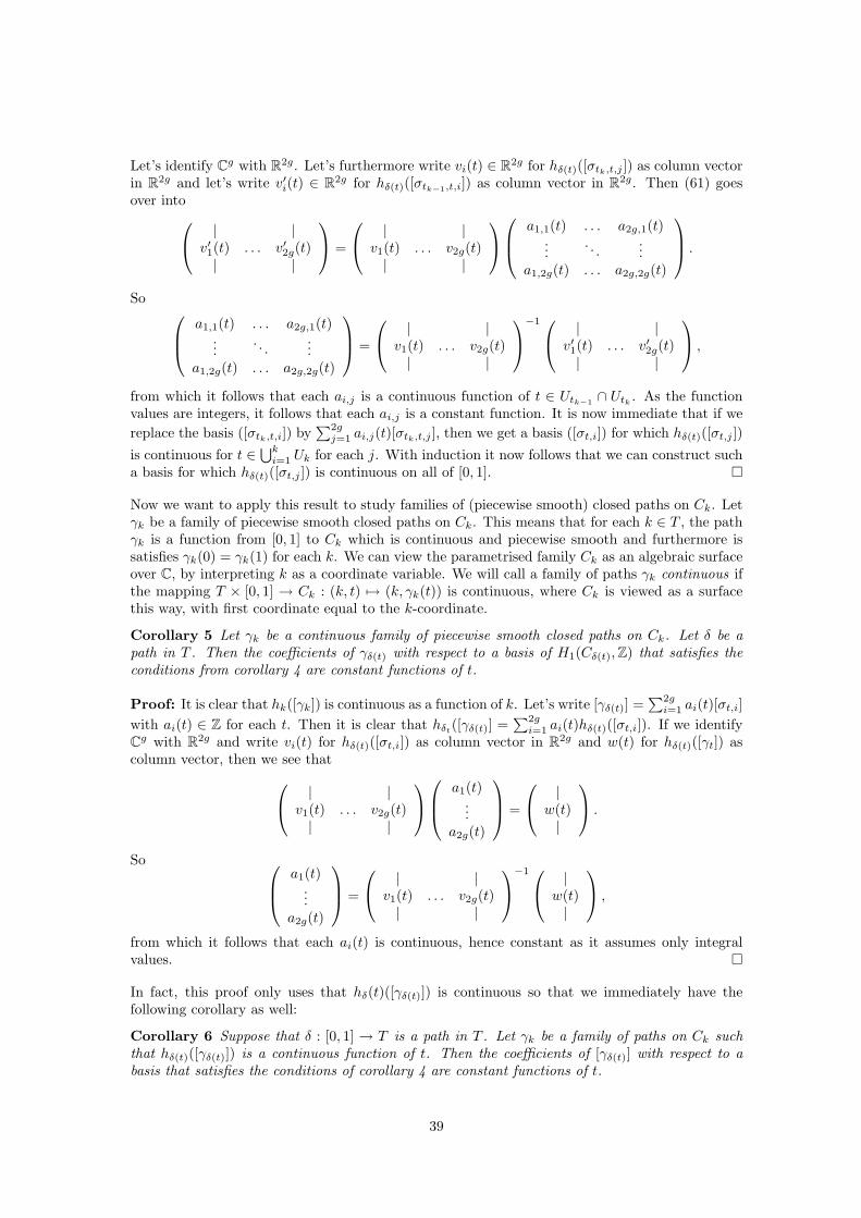
Let’s identify Cg with R2g. Let’s furthermore write vi(t) ∈ R2g for hδ(t)([σtk,t,j ]) as column vectorin R2g and let’s write v′i(t) ∈ R2g for hδ(t)([σtk−1,t,i]) as column vector in R2g. Then (61) goesover into | |
v′1(t) . . . v′2g(t)| |
=
| |v1(t) . . . v2g(t)| |
a1,1(t) . . . a2g,1(t)
.... . .
...a1,2g(t) . . . a2g,2g(t)
.
So a1,1(t) . . . a2g,1(t)...
. . ....
a1,2g(t) . . . a2g,2g(t)
=
| |v1(t) . . . v2g(t)| |
−1 | |v′1(t) . . . v′2g(t)| |
,
from which it follows that each ai,j is a continuous function of t ∈ Utk−1 ∩ Utk . As the functionvalues are integers, it follows that each ai,j is a constant function. It is now immediate that if wereplace the basis ([σtk,t,i]) by
∑2gj=1 ai,j(t)[σtk,t,j ], then we get a basis ([σt,i]) for which hδ(t)([σt,j ])
is continuous for t ∈⋃ki=1 Uk for each j. With induction it now follows that we can construct such
a basis for which hδ(t)([σt,j ]) is continuous on all of [0, 1].
Now we want to apply this result to study families of (piecewise smooth) closed paths on Ck. Letγk be a family of piecewise smooth closed paths on Ck. This means that for each k ∈ T , the pathγk is a function from [0, 1] to Ck which is continuous and piecewise smooth and furthermore issatisfies γk(0) = γk(1) for each k. We can view the parametrised family Ck as an algebraic surfaceover C, by interpreting k as a coordinate variable. We will call a family of paths γk continuous ifthe mapping T × [0, 1] → Ck : (k, t) 7→ (k, γk(t)) is continuous, where Ck is viewed as a surfacethis way, with first coordinate equal to the k-coordinate.
Corollary 5 Let γk be a continuous family of piecewise smooth closed paths on Ck. Let δ be apath in T . Then the coefficients of γδ(t) with respect to a basis of H1(Cδ(t),Z) that satisfies theconditions from corollary 4 are constant functions of t.
Proof: It is clear that hk([γk]) is continuous as a function of k. Let’s write [γδ(t)] =∑2gi=1 ai(t)[σt,i]
with ai(t) ∈ Z for each t. Then it is clear that hδt([γδ(t)] =∑2gi=1 ai(t)hδ(t)([σt,i]). If we identify
Cg with R2g and write vi(t) for hδ(t)([σt,i]) as column vector in R2g and w(t) for hδ(t)([γt]) ascolumn vector, then we see that | |
v1(t) . . . v2g(t)| |
a1(t)
...a2g(t)
=
|w(t)|
.
So a1(t)...
a2g(t)
=
| |v1(t) . . . v2g(t)| |
−1 |w(t)|
,
from which it follows that each ai(t) is continuous, hence constant as it assumes only integralvalues.
In fact, this proof only uses that hδ(t)([γδ(t)]) is continuous so that we immediately have thefollowing corollary as well:
Corollary 6 Suppose that δ : [0, 1] → T is a path in T . Let γk be a family of paths on Ck suchthat hδ(t)([γδ(t)]) is a continuous function of t. Then the coefficients of [γδ(t)] with respect to abasis that satisfies the conditions of corollary 4 are constant functions of t.
39
9 Reciprocal genus 2 curves
Let now K be any field of characteristic 0 again. Suppose that f(x) ∈ K[x] is a polynomial 3with no multiple roots, and that f(0) 6= 0. Then f(x2) has no multiple roots either. Consider thegenus 2 hyperelliptic curve
C : y2 = f(x2). (62)
When a hyperelliptic curve admits this type of equation, we will call it reciprocal. This curvecomes equipped with a map
π : C → P1 : (x, y) 7→ x.
Besides the hyperelliptic involution ι : (x, y) 7→ (x,−y), there are two other interesting involutions:
σ1 : (x, y) 7→ (−x, y) and σ2 : (x, y) 7→ (−x,−y). (63)
Is easy to see that id, ι, σ1, σ2 is a subgroup of AutK(C) which is isomorphic to (Z/2Z)×(Z/2Z).
From now on, suppose that deg(f) = 3 so that the curve has genus 2. Let’s divide out theautomorphisms σ1 and σ2. To do this, we consider the function field K(C) = K(x)[y]/(y2−f(x2))and we have to determine the subfield K(C)σ1 that is fixed by σ1. This is clearly the subfieldK(x2, y). This subfield corresponds to the elliptic curve
E1 : y2 = f(x), (64)
together with the coverφ1 : C → E1 : (x, y) 7→ (x2, y). (65)
We also consider the mapπ1 : E1 → P1 : (x, y) 7→ x.
For the other automorphism σ2, the fixed field is clearly equal to K(x2, xy) = K( 1x2 ,
yx3 ), so that
the elliptic curve and cover are in this case equal to
E2 : y2 = x3f(1x
) and φ2 : C → E2 : (x, y) 7→(
1x2,y
x3
)= [x : y : x3].
For i ∈ 1, 2, the σi-invariant rational functions on C correspond, by construction, to the rationalfunctions on Ei. For example, the function g(x2, y) ∈ K(C)σ1 corresponds to the function g(x, y) ∈K(E1). This will be very important when we will study mahler measures of polynomials that definecurves of genus 2. We will denote the pull-back on C of a function g on Ei by φ∗i (g) and the push-forward on Ei of a σi-invariant function g on C by φi∗(g)
Let’s look at how the morphisms φ1 and φ2 look like on the (v, w)-chart from lemma 14. An easycalculation shows that
φ1(v, w) =(
1v2,w
v3
)= [v : w : v3] and φ2(v, w) = (v2, w).
We can also look at the following map:
φ : C → E1 × E2 : P 7→ (φ1(P ), φ2(P )).
This map is clearly an embedding. Hence we can view C via φ as a closed subvariety of the abeliansurface E1 × E2, as maps between projective varieties are always closed. In fact this shows thatthe Jacobian of C is isogeneous to E1 × E2.
40
The genus 2 curves that we will look at are defined as the zero set of a reciprocal polynomial ofthe form P (x, y) = A(x)y2 +B(x)y + C(x). Note that in that case there is an involution
σ′1 : (x, y) 7→ (1x,1y). (66)
We will show that we can always put the equation of this curve into the standard form (62).By substituting y1 = 2A(x)y + B(x) one gets an equation of the shape y2
1 = f(x). If f(x) herehappens to have square factors, we can move them to the left hand side into the denominator ofy1 and hence we get an equation of the form (59). As P (x, y) is reciprocal, it follows that f(x) isreciprocal as well. We will further subsitute
x =x2 + 1x2 − 1
, y2 = y1(x2 − 1)3
to arrive at an equation of the form (62) for the coordinates x2 and y2. The transformationT (x) = (x + 1)/(x − 1) has the interesting properties that T (T (x)) = x, T (1/x) = −T (x) andT (−x) = 1/T (x) so that the involution σ from (66) goes over into the involution
σ1 : (x2, y2) 7→ (−x2, y2).
Let’s denote the curve defined by the polynomial P by C ′ and the birationally equivalent curvein standard form (62) by C. Also denote the isomorphism between C ′ and C that we obtain viathe above substitutions by
ψ : C ′ → C.
We can also rewrite the involutions ι and σ2 in terms of C ′. Let’s write ι′ and σ′2 respectively.Then ι : (x, y) 7→ (x,−B(x)/A(x) − y) = C(x)/(A(x)y). Because of reciprocity, the fractionC(x)/A(x) will be a power of x, say xm. So that
ι′ : (x, y) 7→(x,xm
y
)σ′2 = σ′1ι
′ : (x, y) 7→(
1x,y
xm
).
Now it becomes clear why the elliptic curve E1 given by (64) is important for computing theMahler measure of P : the differential η(x, y), where x and y are the coordinates on C ′, is invariantunder the action of σ′1. This allows us to rewrite a regulator rC(x, y) to a regulator on E. LetK(C)/K(E1) the quadratic field extension that corresponds to the cover φ1 given by (65). TheGalois group of this field extension is generated by σ∗1 . We can now use the manipulation trick(19) from section 4 to push forward rC(x, y) to E. Namely,
rCx, y([γ]) =12rC (x, yσ(x, y)) ([γ]) =
12rC resK(C)/K(E1)
(NK(C)/K(E1)x, y
)([γ])
=12rE(NK(C)/K(E1)x, y
)([φ1γ]).
Furthermore, we will see in all our examples that (x, y)P is a root of unity for each point P of anonsingular complete model of C ′, where (−,−)P is the tame symbol. From (18) and the well-known fact that a non-constant morphism of nonsingular complete curves is surjective it followsthat ∂P (α) is a root of unity as well. Looking at lemma 6 form section 6 we see that η(α) has allits residues equal to 0.
9.1 Homology
Suppose now that K = C. We want to compute the induced map H1(φ1) : H1(C,Z) → H1(E1,Z)on homology. To do this we will suppose that C and E are given in standard form (62) and (64).We will make a homology basis as in lemma 16 from section 8. Choose α1, α2, α3 ∈ C such that
f(x) = a(x− α21)(x− α2
2)(x− α23),
41

where a is the leading coefficient of f . Then
f(x2) = a(x− α1)(x+ α1)(x− α2)(x+ α2)(x− α3)(x+ α3).
For i ∈ 1, 2, 3, let γ+i : [0, 1] → C−±α1,±α2,±α3 be a closed piecewise smooth path, based at
0, such that the winding number of γ+i around αi is 1 and it is 0 around the other zeroes of f(x2).
Now, let γ−i : [0, 1] → C− ±α1,±α2,±α3 be the path defined as follows: γ−i : t 7→ −γ+i (t). So
γ−i has winding number 1 around −αi and winding number 0 around the other zeroes of f(x2).Set z0 = 0 and choose a point ζ0 = (0, y0) ∈ π−1(0). If we lift paths along π as in subsection 8.1,then lemma 16 shows that the following classes form a basis of H1(C,Z):
a1(C) :=[γ+1 γ
−1
], a2(C) :=
[γ+2 γ
−2
], b1(C) :=
[˜γ−1 γ+2 γ
−2 γ
+3
], b2(C) :=
[γ−2 γ
+3
].
Now, let γ′i : [0, 1] → C − α21, α
22, α
23 be the path defined as t 7→ (γ+
i (t))2. We see that thewinding number of γ′i around α2
i is 1 and it is 0 around the other zeroes of f(x):
indP 2(γ′i) =1
2πi
∫γ′i
dz
z − P 2=
12πi
∫γ+
i
2zdzz2 − P 2
=1
2πi
∫γ+
i
(dz
z − P+
dz
z + P
)= indP (γ+
i ) + ind−P (γ+i ).
We can lift these paths to E1, again as in subsection 8.1, using z0 = 0 and ζ0 = (0, y0). Usinglemma 16, we get the following basis of H1(E1,Z):
a1(E1) =[γ′1γ
′2
], b1(E1) =
[γ′2γ
′3
].
Now, we want to figure out the induced map H1(φ1) on homology. It is not so difficult to see that
π1 φ1 (γ+i γ
−i
)= (γ′i)
2
for i ∈ 1, 2. This implies that H1(φ1)(ai(C)) = 0, an easy way to see this is for example byapplying the map h from equation (60). Also,
π1 φ1 (γ−1 γ
+2
)= γ′1γ
′2 and π1 φ1
(γ−2 γ
+3
)= γ′2γ
′3.
As φ(0, y0) = (0, y0), the map φ sends the base point of the loops in C to the base point of theloops in E. It follows that H1(φ1)(b1(C)) = a1(E1) + b1(E1) and H1(φ1)(b2(C)) = b1(E1). Inconclusion,
H1(φ1) (c1a1(C) + c2a2(C) + c3b1(C) + c4b2(C)) = c3a1(E1) + (c3 + c4)b1(E1). (67)
42
10 The family Pk(x, y) = y2 + (x4 + kx3 + 2kx2 + kx + 1)y + x4
Let C ′k be the family curves defined by the polynomial Pk(x, y) = y2 + (x4 + kx3 + 2kx2 + kx +1)y + x4. If k ∈ C, we can view this as a curve over the field Q(k). The curve C ′k has genericallygenus 2, as one can compute with the Riemann-Hurwitz formula. Hence it is a hyperelliptic curve.We do not even need to know the Riemann-Hurwitz formula nor the fact that curves of genus2 are always hyperelliptic to make these conclusions as we can write the curve in the followingnormal form:
Ck : y2 = f(x2),
wheref(x) = (k2 + k)x3 + (−2k2 + 5k + 4)x2 + (k2 − 5k + 8)x− k + 4.
A birational map between the curves C ′k and Ck can be given by
ψ : C ′k → Ck : (x, y) 7→(x+ 1x− 1
,4(y2 − x4)
y(x− 1)3(x+ 1)
), (68)
whose inverse is equal to
ψ−1 : Ck → C ′k : (x, y) 7→(x+ 1x− 1
,2xy − (2k + 1)x4 + (2k − 6)x2 − 1
(x− 1)4
). (69)
So the elliptic curve E that we get by dividing out the involution σ from (66) is
E : y2 = (k2 + k)x3 + (−2k2 + 5k + 4)x2 + (k2 − 5k + 8)x− k + 4.
Lemma 17 If K = C, then Ck has genus 2 for k ∈ C−−1, 0, 4, 8. Furthermore, Ck has genus1 if k ∈ −1, 4, it has genus 0 if k = 8 and it is a reducible curve consisting of 2 irreduciblecomponents of genus 0 if k = 0.
Proof: The discriminant of f(x2) is equal to 222k3(k − 8)2(k − 4)(k + 1). So f(x2) has degree 6and no multiple roots if k ∈ C− −1, 0, 4, 8, so lemma 15 shows that Ck has genus 2.
Let’s look at what happens if k ∈ −1, 0, 4, 8. If k = −1, then f(x) = −3x4 + 14x2 + 5, so Ckhas genus 1. If k = 0, then f(x) = 4(x2 + 1)2. This means that Ck is not even irreducible, it has2 irreducible components, each of genus 0. If k = 4, then f(x) = 4x2(5x4 − 2x2 + 1), so Ck isbirationally equivalent to the curve y2 = 5x4 − 2x2 + 1, hence it has genus 1. And if k = 8, thenf(x) = 4(3x2 + 1)2(2x2 + 1), so Ck is birationally equivalent to y2 = 2x2 + 1, hence of genus 0.
Next, we will compute the values of the tame symbols (x, y)P on C ′k (for a definition of the tamesymbol, see formula (17) in section 4). Being coordinates, x and y are still functions on a completenonsingular model C ′k for C ′k.
Lemma 18 For all P ∈ C ′k, the tame symbol (x, y)P is a root of unity.
Proof: If ordP (x) = 0 and ordP (y) = 0 then it is clear that (x, y)P = 1. So suppose now thatordP (x) > 0. If ordP (y) < 0 then on one hand, ordP (y2+(x4+kx3+kx2+kx+1)y) = 2 ordP (y) <0, but on the other hand, ordP (y2 + (x4 + kx3 + kx2 + kx + 1)y) = ordP (x4) > 0, so this is notpossible. If ordP (y) > 0, then P is the point (0, 0), which is a nonsingular point of C ′k. We seenow that ordP (y) = ordP (y2 + (x4 + kx3 + kx2 + kx+ 1)y) = ordP (x4) = 4 ordP (x). Hence
(x, y)P =
(x4
y
∣∣∣∣(0,0)
)ordP (x)
=(−(y + x4 + kx3 + 2kx2 + kx+ 1)|(0,0)
)ordP (x)= ±1
43

so the claim follows. The subcase ordP (y) = 0 is left. Here, ordP (y+x4 + kx3 + 2kx2 + kx+ 1) =ordP (y2 +(x4 + kx3 + kx2 + kx+1)y) = ordP (x4) > 0. So P is the nonsingular point (0,−1). Wecan now see that
(x, y)P =1
y(P )ordP (x)= (−1)ordP (x),
which is a root of unity as well.
Let’s now look at the case ordP (x) < 0. Remind that σ′1 is the automorphism (x, y) 7→ (1/x, 1/y)on C ′k. From (17) it follows immediately that
(x, y)P =(
1x,1y
)P
= (x σ′1, y σ′1)P = (x, y)σ′1(P )
and ordσ′1(P )(x) = − ordP (x) > 0 so we have reduced the problem to a case we have alreadyproved.
So we are left with the case ordP (x) = 0. There are two subcases to examine, namely ordP (y) > 0and ordP (y) < 0. As above, the former subcase implies the latter one by applying σ′1. Thus weassume that ordP (y) > 0. But then we get a contradiction from ordP (x4) = ordP (y2 +(x4 +kx3 +kx2 + kx+ 1)y) ≥ ordP (y) > 0.
10.1 Construction of closed paths γk on C ′k
Let’s now find out for which k ∈ R there exists a function y+(x) for the polynomial Pk(x) thatsatisfies conditions 1 and (10) from section 2.1. The equation Pk(x, y) = 0 is a quadratic equationfor the variable y, with discriminant equal to
Dk(x) = (x+ 1)2(x2 + (k − 2)x+ 1)(x4 + kx3 + 2(k + 1)x2 + kx+ 1). (70)
According to the abc-formula, we have to take the square root of this discriminant. In this abc-formula we see that
ak(x) = 1, bk(x) = x4 + kx3 + 2kx2 + kx+ 1, ck(x) = x4.
It is well known (see for example chapter 10 in [11]) that the square root of a holomorphic funtionf exists on an open set U if and only if for every closed path γ in U , the total winding numberof γ around the zeroes of f (counting with multiplicities) is divisible by 2. So if Dk(x) has anodd number of zeroes with |x| < 1 we do not expect that there exists a function y satisfying bothcondition 1 and (10). The following lemma and corollary show that this is indeed not possible:
Lemma 19 Let C = z ∈ C : |z| = 1 be the unit circle in C. Let f be a polynomial with realcoefficients without multiple zeroes. Suppose that f has an odd number of zeroes of absolute valuestrictly less than 1. Suppose furthermore f(1) 6= 0 and f(−1) 6= 0. Then there does not exist acontinuous function g : C → C such that g(x)2 = f(x) and g(x) = g(x) for each x ∈ C.
Proof: Suppose that such a function g does exist. Let X = (x, y) ∈ C2 : y2 = f(x) and defineπ : X → C : (x, y) 7→ x. As f has no multiple zeroes, X has no singular points. As the number ofzeroes of f is finite we can find a number c with 0 < c < 1 such that |x| < c for every zero x of fof absolute value strictly less than 1 and |x| > 1/c for every zero x of f of absolute value striclygreater than 1. Define the path
γ1 : [0, 1] → X : t→ (exp(πit), g(exp(πit)))
44
(so γ1 is a lift of the upper half of the circle C to C ′k). Then clearly γ1 is path-homotopic to a pathγ′2, not passing through any points with y-coordinate equal to 0 and such that the x-coordinatesof all the points it passes satisfy c < x < 1/c. We also have a closed path
γ2 : [0, 1] → X : t→ (exp(2πit), g(exp(2πit))) .
Clearly, γ2 is homotopic to the path
γ′2 : [0, 1] → X : t→γ′1(2t) if 0 ≤ t < 1
2 ;γ′1(2− 2t) if 1
2 < t ≤ 1,
where (x, y) = (x, y), because g(x) = g(x) for each x ∈ C. We can now look at the pathπ γ′2 : [0, 1] → C, it does not meet any zeroes of f . The total winding number around the zeroesof f is odd, since the number of zeroes x with |x| < 1 is odd and the zeroes of f with |x| = 1 thatcontribute to the total winding number come in complex conjugate pairs. But it is well-knownthat any path with odd total winding number around the zeroes of f lifts to a path which is notclosed. Hence we have a contradiction.
Corollary 7 If Dk(x) has an odd number of zeroes with |x| < 1, with k real, then there does notexist a function y satisfying both condition 1 and (10).
Proof: Suppose that such a function y does exist. Clearly Dk(x) satisfies the conditions for f inlemma 19. Taking g(x) = 2(y(x) + bk(x)) in this lemma we get a contradiction.
If the number of zeroes of Dk(x) with |x| < 1 is even, then we will construct a set U as follows:take the entire complex plane C, and remove from it some so-called branch cuts. We can drawthese branch cuts as follows: for each zero x0 of odd multiplicity of Dk(x) with |x0| < 1 we drawthe ray λx0 : 0 ≤ λ ≤ 1. For each zero x0 of odd multiplicity of Dk(x) with |x0| ≥ 1 we drawthe ray λx0 : λ ≥ 1. If it happens that there are no zeroes with |x| < 1 then we still removethe point 0. As the set of zeroes is invariant under complex conjugation, these branch cuts areinvariant under conjugation as well.
Lemma 20 If Dk(x) has an even number of zeroes with |x| < 1 then the open set U constructedabove satisfies U = U (of course we mean the complex conjugation here and not the toplogicalclosure) and we can take a square root of Dk(x) on U as a holomorphic function. Furthermore,the function
√Dk(x) is defined over R, which means that it satisfies
√Dk(x) =
√Dk(x) for all
x ∈ U .
Proof: The invariance of U under complex conjugation follows immediately from the constructionof U . As the number of zeroes of Dk(x) with |x| < 1 is finite we can find a number c with 0 < c < 1such that |x| < c for every zero x of Dk(x) of absolute value strictly less than 1. Because 0 6∈ U ,the circle C = z ∈ C : |z| = c is a subset of U . We can now also see that this circle is adeformation retract of U , define the retraction as follows:
U × [0, 1] → U : (z, t) 7→ (1− t)z + tcz
|z|.
It follows now that the closed path γ : [0, 1] → U : t 7→ c exp(2πit) defines a generator of H1(U,Z).Because the number of zeroes of Dk(x) with |x| < c is even, the total winding number of γ aroundthe zeroes of Dk(x) is even. Hence the total winding number of every closed path in U aroundthe zeroes of Dk(x) is even. Hence we can define
√Dk(x) as a holomorphic function on U . There
are two choices for√Dk(x), fix one of them.
45

Now, consider the function
f : U → C : z 7→√Dk(z)(√Dk(z)
) .This function is well-defined because U = U and U does not contain any zeroes of Dk(x). AsDk(x) is defined over R, it follows that f(z)2 is identically 1 on U . So f takes the values 1 and−1. The set U is connected, because it is homotopy-equivalent to C. So f is constant as f iscontinuous, hence f is either identically 1 or identically −1.
To examine whether f is identically 1 or −1 we distinguish three cases: k > 0, k < 0 and k = 0.Let’s start with the case k > 0. Let’s try to prove that Dk(x) has no positive real zeroes. From thewell-known arithmetic-geometric mean inequality it follows that x2 + 1 ≥ 2x for positive real x.Hence the factor x2 +(k−2)x+1 of (70) is strictly positive for x > 0. It’s clear that the other twofactors have no zeroes for x > 0 either. This implies, by construction of U , that the set of positivereal numbers is a subset of U . As Dk(x) has leading coefficient 1, we know that there is x0 > 0 suchthat Dk(x0) > 0. This implies that
√Dk(x0) is real. Hence
√Dk(x0) =
√Dk(x0) =
√Dk(x0)
or, equivalently, f(x0) = 1. Hence f is identically 1 in this case, which implies the claim that√Dk(x) is defined over R.
Let’s now check the case k < 0. There is a double zero x = −1 of Dk(x) on the negativepart of the real line. We’ll show that this is the only zero on R<0. It’s clear that the factorx2 + (k − 2)x + 1 is strictly positive for x < 0. From the arithmetic-geometric mean inequalityit follows that k(x3 + x) = |k|(|x|3 + |x|) ≥ 2|k||x|2 = −2kx2 for x < 0. Hence the factorx4 + kx3 + 2(k + 1)x2 + kx+ 1 is strictly positive for x < 0. So x = −1 is the only zero of Dk(x)with x < 0. This is a zero of even multiplicity, so the negative real line is part of U . As Dk(x)has even degree and leading coefficient equal to 1, there is an x0 < 0 with Dk(x0) > 0 and nowfor the same reason as above,
√Dk(x) is defined over R.
In the case k = 0, the polynomial Dk(x) is the square of the polynomial x4− 1. So√Dk(x) must
be x4 − 1 or −x4 + 1, which are both defined over R.
We will now examine what kind of implications this has on the functions y(x) as solution ofPk(x, y) = 0. In the general case we get the following picture: there is a function y(x) such that|y(x)| = 1 for x on a left part of the unit circle (left to the roots of Dk(x)) and |y(x)| > 1 for x onthe right of these roots on the unit circle.
Let U ′ be the union of U with the set of zeroes of Dk(x). At the zeroes of Dk(x) we define√Dk(x)
to be 0, so that√Dk(x) is continuous there. By the abc-formula we find two functions y that
satisfy condition 1:
y(x) =−bk(x)±
√Dk(x)
2ak(x)=
12
(−(x4 + kx3 + 2kx2 + kx+ 1)±
√Dk(x)
).
It is now immediate that y(x) = y(x), so that y(x) is defined over R. We still don’t know whetherone of these two functions satisfies |y(x)| ≥ 1 for |x| = 1, but we will examine that later. One cancompute
√Dk(x) as follows: fix a point x0 ∈ U , together with a choice of
√Dk(x0). Choose a
path γ from x0 to x, lying in U . Then√Dk(x) =
√Dk(x0) · exp
(12
∫γ
d logDk(x))
=√Dk(x0) · exp
(12
∫γ
D′k(x)
Dk(x)dx
).
46
So we should find out for which k, the discriminant Dk(x) has an even number of zeroes within thedisc D(0, 1). As Dk(x) is a reciprocal polynomial, the mapping α 7→ 1/α is an involution on themultiset of zeroes. This implies that the number of zeroes inside D(0, 1) is equal to the number ofzeroes outside D(0, 1), so we only have to figure out how many zeroes there are on the unit circle.We will consider a number of cases: k > 4, k = 4, 0 < k < 4, k = 0, −1 < k < 0, k = −1 andk < −1.
Let’s start with the case k > 4. We will show that the double zero x = −1 are the only zeroes onthe unit circle. As the degree of Dk(x) is 8, we see that there are 3 zeroes in D(0, 1), so in thiscase we do not expect that a nice function y exists. Indeed, for these values of k, the polynomialPk(x) does not seem to satisfy Boyd’s conjecture (see [4]). As the factorisation (70) shows, wemust look for zeroes of x2 + (k − 2)x + 1 and for zeroes of x4 + kx3 + 2(k + 1)x2 + kx + 1. Thediscriminant of x2 + (k − 2)x + 1 is strictly positive if k > 4 so this factor has two disctinct realzeroes, whose product is 1. Hence they cannot lie on the unit circle. Now we have to study theequation x4 + kx3 + 2(k + 1)x2 + kx + 1 = 0. After dividing both sides by x2 and substitutingw = x+ 1/x this equation goes over into the equation
w2 + kw + 2k = 0. (71)
It is easily verified that x is on the unit circle if and only if w is a real number with |w| ≤ 2. So wemust show that there are no real roots of (71) with |w| ≤ 2. The graph of f(w) = w2+kw+2k, as afunction on the reals, is a convex parabola. As k ≥ 4, the top of the parabola is at w = −k/2 ≤ −2.Because f(−2) = 4 > 0, it follows that f(w) > 0 for any w ≥ −2, so f has no zeroes on [−2, 2]hence the factor x4 + kx3 + 2(k+ 1)x2 + kx+ 1 has no zeroes on the unit circle, which is what wewanted to prove.
In the case k = 4, the zero x = −1 of Dk(x) has multiplicity 4: another 2 of these zeroes arecoming from the factor x2 + (k − 2)x + 1. For the same reason as in the case k > 4, the factorx4 + kx3 +2(k+1)x2 + kx+1 has no zeroes on the unit circle. So the number of zeroes in D(0, 1)is 2 in this case. Hence by lemma 20 there exists a function y satisfying condition 1 and (10).
Now we have to figure out whether there exists such a function y which satisfies |y(x)| ≥ 1 for allx ∈ C with |x| = 1. After choosing branch cuts and hence an open set U , there are exactly twoholomorphic choices for
√Dk(x) on U , hence two choices for y(x) on U ′ where U ′ denotes the
union of U and the zero set of Dk(x). We can compute the two possible values for y(1): they areroots of the equation y2 + 18y + 1 = 0. The discriminant of this equation is strictly positive andthe product of the two roots is 1. Hence this equation has exacly one real root y with |y| > 1.Let y+(x) be the choice of y(x) with y(1) equal to this root and let y−(x) be the other choiceof y(x). Set the choice of
√Dk(x) in such a way that y+(x) = (−b(x) +
√Dk(x))/(2a(x)) and
y−(x) = (−bk(x)−√Dk(x))/(2ak(x)).
We will show that |y+(x)| ≥ 1 for all x ∈ C with |x| = 1. Let’s start with finding out for which xon the unit circle the absolute value of y+(x) is exactly equal to 1. It is clear that y+(x)y−(x) = x4
for each x ∈ U ′. Hence
|y+(x)| · |y−(x)| = 1 for all x with |x| = 1. (72)
So, for x on the unit circle, |y+(x)| = 1 if and only if |y+(x)| = |y−(x)| if and only if | −bk(x) +√Dk(x)| = | − bk(x) −
√Dk(x)| if and only if the complex numbers bk(x) and
√Dk(x) are
perpendicular as vectors in the plane if and only if Dk(x) = 0 or bk(x)/√Dk(x) ∈ iR if and only
ifDk(x) = 0 or (bk(x))2/Dk(x) ∈ R≤0.
It may seem like a coincidence that such a complex number is negative real but in fact the number(bk(x)2)/Dk(x) is always real if |x| = 1. This can be easily verified by checking that (bk(x)2)/Dk(x)
47

is its own complex conjugate, using that x = 1/x. Let f(x) = (bk(x)2)/Dk(x) as a function fromthe unit circle to R. We want to know at which points f changes sign if we walk on the unitcircle. This can only happen at a zero or pole of odd multiplicity, hence at a zero of Dk of oddmultiplicity. As we are in the case k = 4, we have seen above that Dk has only 1 zero on the unitcircle, and it is of multiplicity 4. After substituting x = 1, one sees that, for each x on the unitcircle, Dk(x) = 0 or f(x) ≥ 0. So the only points on the unit circle where |y+(x)| = 1 are thezeroes of Dk and the zeroes of bk. Let’s compute the zeroes of bk(x). After dividing the equationbk(x) = 0 by x2 and substituting w = x+ 1/x, this equation goes over into
w2 + kw + 2(k − 1) = 0. (73)
In this particular case k = 4 and one can see that the discriminant is negative, so it has no realroots for w hence bk(x) has no zeroes on the unit circle. Hence, for x on the unit circle,
|y+(x)| = 1 if and only if x = −1.
Now from the fact that |y+(x)| is a continuous function and |y+(1)| > 1, it follows that |y+(x)| ≥ 1for all x ∈ C with |x| = 1.
Let’s now go to the case 0 < k < 4. In this case the discriminant of the factor x2 + (k− 2)x+ 1 isstrictly negative so the two zeroes are conjugate to each other. The product of the two zeroes ofx2 + (k− 2)x+ 1 is 1 so these zeroes lie on the unit circle. Let’s check the factor x4 + kx3 + 2(k+1)x2 +kx+1 now. Again, if x is a zero with |x| = 1 and w = x+1/x, then w should be a real rootof absolute value at most 2 of (71). However, the discriminant of w2 + kw + 2k equals k(k − 8)so this is negative as 0 < k < 4. So (71) cannot have any real roots at all. So on the unit circleDk(x) has the double zero x = −1 and two zeroes coming from x2 + (k − 2)x+ 1. So there are 4zeroes on the unit circle, hence Dk(x) has 2 zeroes in D(0, 1). So also in this case there exists bylemma 20 a function y(x) satisfying condition 1 and (10).
Again, we have to figure out whether there exists a function y(x) with |y(x)| ≥ 1 for all |x| =1. We will do a similar investigation as in the previous case. For y(1) we get the equationy2 + (4k + 2)y + 1 = 0. The discriminant of this equation is stricly positive and the product ofthe roots is 1. So there is a root with |y(1)| > 1 and the other root has |y(1)| < 1. Again, definey+(x) to be the y-function with |y+(1)| > 1 and y−(x) to be the other one. As before we choose√Dk(x) such that y+(x) = −bk(x)/2 +
√Dk(x)/2. Again, |y+(x)| = 1 for x on the unit circle if
and only Dk(x) = 0 or the real number bk(x)2/Dk(x) is negative or 0. At x = 1 the value of thisfunction is (4k + 2)2/(16k(k + 1)) > 0. If we walk around the unit circle, bk(x)2/Dk(x) switchessign at the zeroes of Dk(x) of odd multiplicity, hence at the two zeroes that come from the factorx2 + (k − 2)x + 1. So, walking around the unit circle from 1 to 1, the function bk(x)2/Dk(x)between these 2 zeroes of Dk(x). Let’s now check whether bk(x) has zeroes on the unit circle.Suppose bk(x) has a zero x0 on the unit circle. Again this zero corresponds to a real root w0 of(73) of absolute value at most 2. If this equation has real roots, then the discriminant k2− 8k+ 8is nonnegative and the largest real root is equal to (−k +
√k2 − 8k + 8)/2. The real parts of the
zeroes of Dk(x) on the unit circle are −(k − 2)/2. From the fact that <x0 = w0/2 it follows that
<x0 ≤−k +
√k2 − 8k + 84
<−k +
√k2 − 8k + 16
4= −k − 2
2,
where in the last equality we use that k < 4 so√k2 − 8k + 16 = 4 − k. We see that if bk(x) has
zeroes on the unit circle, then they must lie on the left of the zeroes of Dk(x) on the unit circlethat are not −1, so this does not give additional points where |y+(x)| = 1.
So, for x on the unit circle, |y+(x)| = 1 if and only if x lies on the left of the zeroes of Dk(x) onthe unit circle that are not -1. From the continuity and the fact that |y+(1)| > 1 it follows now
48

that |y+(x)| ≥ 1 for all x on the unit circle.
The case k = 0 is not very interesting: we can use lemma 2 and identity (4), together with lemma1 to compute m(Pk(x, y)):
m(Pk(x, y)) = m(y2 + (x4 + 1)y + x4) = m(y + 1) +m(y + x4) =
= m(y + x4) = m(y + x) = m(y + xy) = m(y) +m(x+ 1) = 0.
Let’s examine the case −1 ≤ k < 0 now. The discriminant of x2 + (k − 2)x + 1 is striclypositive in this case so this factor does not have any zeroes on the unit circle. Again the zeroesof x4 + kx3 + 2(k + 1)x2 + kx + 1 on the unit circle are in a 2-1 correspondence to the realroots of (71) of absolute value at most 2. Set f(w) = w2 + kw + 2k. One can easily verify thatf(−2) > 0, f(0) < 0 and f(2) ≤ 0 so that (71) has two real roots in the interval [−2, 2]. Hencex4 + kx3 + 2(k + 1)x2 + kx + 1 has 4 zeroes on the unit circle. Together with the double zerox = −1, there are 6 zeroes of Dk(x) on the unit circle. Hence there is 1 zero inside the unit circle,so there is no function y(x) that satisfies condition 1.
Let’s next assume that k < −1. The disciminant of x2+(k−2)x+1 is strictly positive so this factordoes not have zeroes on the unit circle. Let’s again figure out how many zeroes the polynomialf(w) = w2 + kw + 2k has on the interval [−2, 2]. As is easily seen, f(−2) > 0 and f(0) < 0 sof(w) has a zero between −2 and 0. We can also see that f(2) < 0 so the other zero of f(w) mustbe stricly greater than 2. Hence the factor x4 + kx3 + 2(k + 1)x2 + kx + 1 of Dk(x) has exactly2 zeroes on the unit circle. So Dk(x) has 4 zeroes on the unit circle, 2 zeroes with |x| < 1 and 2zeroes with |x| > 1. So in this case there exists a nice function y(x) that satisfies condition 1 and(10).
Again for y(1) the equation y2 +(4k+2)+1 = 0 holds, which has a strictly positive discriminant.Hence there is a root with |y(1)| > 1 and one with |y(1)| < 1. Let, as in the previous cases, y+(x)be the choice of y(x) with y(1) > 1 and y−(x) be the choice of y(x) that has y(1) < 1. Also choose√Dk(x) such that y+(x) = −bk(x)/2+
√Dk(x)/2. As above, |y+(x)| = 1 for x on the unit circle if
and only if Dk(x) = 0 or the real number bk(x)2/Dk(x) is negative. The same arguments as beforeshow that this function is negative or 0 for x on the unit circle where <x is smaller than the realpart of the roots of Dk(x) on the unit circle, that are not equal to -1. Again we have to find outwhere bk(x) can vanish on the unit circle. Suppose that bk(x) has a zero x0 on the unit circle. Thenthis zero corresponds to a root w0 of (73) in [−2, 2] and <x0 = w0/2. A zero x1 of Dk(x) on theunit circle, not equal to -1, comes from the factor x4 +kx3 +2(k+1)x2 +kx+1 hence correspondsto a root w1 of (71) in [−2, 2] and <x1 = w1/2. The roots of (73) are (−k+
√k2 − 8k + 8)/2 and
(−k −√k2 − 8k + 8)/2. From the fact that (−k +
√k2 − 8k + 8)/2 > 2 it follows that
w0 =−k −
√k2 − 8k + 82
.
Similarly,
w1 =−k −
√k2 − 8k2
and we see that w0 < w1 hence <x0 < <x1. So bk(x) does not give us additional points on theunit circle where |y+(x)| = 1.
So for x on the unit circle, |y(x)| = 1 if and only if x lies on the left of the zeroes of Dk(x) on theunit circle that are not -1 (we say that a complex number z lies on the left of a complex numberw if <z < <w). As before we see that |y+(x)| ≥ 1 for all x on the unit circle.
Let’s summarize all this in the following proposition:
49

Proposition 5 For k ∈ ]−∞,−1[ ∪ ]0, 4] there exists an open set U ⊂ C and a function holo-morphic function y+(x) on U that satisfy the following conditions:
• U = U ,
• Pk(x, y(x)) = 0 for all x ∈ U ,
• condition 1 from section 2.1,
• y+(x) = y+(x) for all x ∈ U ,
• |y+(x)| ≥ 1 for all x ∈ U of absolute value 1.
The function y−(x) satisfies the first 3 conditions from proposition 5 as well. And because of (72),which holds for any k ∈ ]−∞,−1[ ∪ ]0, 4], the function y−(x) satisfies
|y−(x)| ≤ 1 for all |x| = 1.
For any x0 ∈ U ′, the zeroes of the polynomial P (x0, y) are y+(x0) and y−(x0). Let γk be the pathon C ′k(C) defined by equation (9) from section 2.1. Then equation (11) from the same sectionshows that
m(Pk(x)) = − 12πi
∫γ
η(x, y),
where η(x, y) is defined by formula (34) from section 6.
Let’s figure out now whether γk lifts to a closed path on a nonsingular model C ′k of C ′k. Toverify this, only the singular points on C ′k(C) with |x| = 1 are interesting to look at. A standardcalculation shows that the following points (x, y) with |x| = 1 are singular:
(x, y) = (−1,−1) for all k,(x, y) = (1, 1) if k = −1,
(x, y) = (−± i,−1) and (x, y) = (1,−1) if k = 0.
Luckily, we have excluded the cases k = −1 and k = 0 above, so that we only have to concentrateon the singularity (−1,−1). To study the lifting of γk to C ′k at this point, we only need to looklocally at the blow-up of C ′k at (−1,−1). We can do this at follows: define
Rk(x, y) = y2 + (x3 + (k − 4)x2 + (−k + 6)x− 4)y − kx+ k.
Then the following map is locally the blow-up of C ′k at (−1,−1):
ρ1 : Z(Rk) → C ′k : (x, y) 7→ (x− 1, xy − 1),
whose rational inverse is
ρ−11 : C ′k − (−1,−1) → Z(Rk) : (x, y) 7→
(x+ 1,
y + 1x+ 1
). (74)
The geometric points in Z(Rk) above (−1,−1) are (0, 2 ±√
4− k), these points are defined overQ(√
4− k). If m is the maximal ideal (x, y) in Q(√
4− k)[x, y], then
Rk(x, y + 2±√
4− k) ≡(3(4− k)± (6− k)
√4− k
)x+ 2
√4− k y modm2.
This shows that the points (0, 2±√
4− k) are nonsingular points of Z(Rk) when k 6= 4. If k = 4then we can further blow up Z(Rk) at the point (0, 2). We get the polynomial
Q4(x, y) = y2 + (x2 + 2)y + 2x,
50
and a mapρ2 : Z(Q4) → Z(R4) : (x, y) 7→ (x, xy + 2),
with rational inverse
ρ−12 : Z(R4)− (0, 2) → Z(Q4) : (x, y) 7→
(x,y − 2x
).
The points above (0, 2) ∈ Z(R4) are (0, 0) and (0,−2), who are clearly nonsingular. We get acomposed map
ρ1 ρ2 : Z(Q4) → C ′4 : (x, y) 7→ (x− 1, x2y + 2x− 1),
with rational inverse equal to
(ρ1 ρ2)−1 : C ′4 − (−1,−1) → Z(Q4) : (x, y) 7→(y − 2x− 1(x+ 1)2
). (75)
To study the lifting of the path γk to the blow-up, we will examine the case k 6= 4 first. The function√Dk(x) constructed above is holomorphic at x = −1. If we compute its Taylor expansion at this
point, then we see that√Dk(x) = 2
√4− k(x + 1) + O((x + 1)2) for an appropriate choice of√
4− k. Also, bk(x) = 2− 4(x+ 1) +O((x+ 1)2). From this it follows that
y+(x) + 1x+ 1
= 2 +√
4− k +O(x+ 1).
Comparing this with (74), we see that the blow-up lifts γk at the point (−1,−1) ∈ C ′k(C) to thepoint (0, 2+
√4− k) ∈ Z(Rk)(C), from which it follows that the lifting of γk to C ′k is still a closed
path.
It remains to study the case k = 4. Again, we compute the Taylor expansion of√D4(x) at
x = −1, but now with an extra term. It turns out to be√D4(x) = 2ε(x+ 1)2 +O(x+ 1)3, for an
appropriate choice of ε ∈ 1,−1. And b4(x) = 2− 4(x+ 1) + 2(x+ 1)2 +O((x+ 1)3). It followsthat
y+(x)− 2x− 1(x+ 1)2
= ε− 1 +O(x+ 1).
As above, comparing this with (75), we can conclude that the lifting of γ4 to C ′4 is still closed.
10.2 Degenerate cases
In our family of curves, there are some degenerate cases, as lemma 17 shows. It turns out thatthese cases are easier to study than the rest. We will be able to express the Mahler measure interms of the L-series of an odd Dirichlet character, defined by (2). Generally for any nontrivialDirichlet character we can say the following: let m be the conductor of χ (i.e. the smallest positiveinteger such that χ is periodic with period m). Let p be the parity of χ, which is defined as 0 ifχ(−1) = 1 and 1 if χ(−1) = −1. Now define the following function:
Λ(χ, s) :=(mπ
)s/2Γ(s+ p
2
)L(χ, s).
It satisfies the equation
Λ(χ, s) =τ(χ)ip√m
Λ(χ, 1− s),
where τ(χ) is the famous Gauss sum:
τ(χ) =m−1∑k=0
χ(k)e2πik
m .
For a proof of this, see chapter 7 of [16]. This functional equation immediately implies the equation(3) if χ = χ−m.
51
10.2.1 The case k = 8
Let’s study the case k = 8. Above it is shown that y cannot be nicely expressed in terms of x.However, in this case this will turn out not to be a big problem. We can factor D8(x) as follows:
D8(x) = (x+ 1)2(x2 + 4x+ 1)2(x2 + 6x+ 1).
So in order to define a useful square root of D8(x) we will have to define a useful square root ofx2 +6x+1. After that we can put
√D8(x) = (x+1)(x2 +4x+1)
√x2 + 6x+ 1. We draw a branch
cut on the negative part of the real axis. Then on C−R<0 we can define a square root of x2+6x+1and then we can use the abc-formula to express y in terms of x. We choose
√x2 + 6x+ 1 to be
that squareroot of x2 + 6x+ 1 such that |y(1)| > 1. We see that√x2 + 6x+ 1 = 2
√2 for x = 1.
The corresponding y-function will be denoted y+ again. The only zero of D(x) on the unit circleis the double zero x = −1. So again a similar argument as given in subsection 10.1 shows that|y+(x)| > 1 for x with |x| = 1 and x 6= −1.
The resulting function y+ is continuous now, so the path of integration seems to be closed. How-ever, if we blow up the singularity (x, y) = (−1,−1), the blown up path will not be closed anymore.This has to do with the fact that
√x2 + 6x+ 1 is not continuous at x = −1. Let’s try to figure out
the behaviour of√x2 + 6x+ 1 above and below x = −1. We will first show that if
√x2 + 6x+ 1 ∈
R, then x ∈ R. So assume that√x2 + 6x+ 1 ∈ R. Then (x+ 3)2 − 8 = x2 + 6x+ 1 ∈ R≥0. This
implies that (x+3)2 ∈ R≥0. This is only possible if x ∈ R. The Taylor expansion of√x2 + 6x+ 1
at x = 1 starts with 2√
2 +√
2(x− 1) +O((x− 1)2). So =√x2 + 6x+ 1 > 0 for x with =x > 0 in
a sufficiently small neighbourhood of 1. As =√x2 + 6x+ 1 6= 0 for =x > 0 and x ∈ C : =x > 0
is a connected set, we see that =√x2 + 6x+ 1 > 0 if =x > 0. Similarly =
√x2 + 6x+ 1 < 0 if
=x < 0. It follows now that
limx→−1=x>0
√x2 + 6x+ 1 = 2i and lim
x→−1=x<0
√x2 + 6x+ 1 = −2i (76)
because the limits clearely exist and take values in −2i, 2i.
Let’s consider the path
γ :]0, 1[→ C ′8 : t 7→ (− exp(2πit), y+(− exp(2πit))) .
Blowing up the singularity (−1,−1) will break up this path (that’s why we consider it as a functionof the open interval ]0, 1[ instead of the closed interval [0, 1]). From (11) it follows that the followingformula holds:
m(P8) = − 12π
∫γ
η(x, y).
Now we want to know what the path γ looks like after a transformation by the birational map ψin (68). An easy calculation using (76) shows that
limt7→0
ψ(γ(t)) = (0, 2i) and limt7→1
ψ(γ(t)) = (0,−2i).
So ψ γ is a path on Ck from (0, 2i) to (0,−2i). In view of (69), we see that
m(P8) = − 12π
∫ψγ
η
(x+ 1x− 1
,2xy − 17x4 + 10x2 − 1
(x− 1)4
).
As C8 is a curve of genus 0, it is birationally equivalent to P1. We identify P1(C) with C ∪ ∞.We take the following birational map:
φ : Ck → P1 : (x, y) 7→ iy + (6− 6i)x3 − 6x2 − (2− 2i)x+ 2iy − (6 + 6i)x3 + 6x2 + (2 + 2i)− 2
52

with inverse equal to
φ−1 : P1 → Ck : z 7→(
(1− i)zz2 − i
,2(−iz6 + 5z4 + 5iz2 − 1)
(z2 − i)3
).
We have chosen this birational map in such a way that the path ψ γ goes over into a path from0 to ∞, as one can easily verify. One can also easily verify that
(φ−1)∗(x+ 1x− 1
)= − (z + 1)(z − i)
(z − 1)(z + i)
and
(φ−1)∗(
2xy − 17x4 + 10x2 − 1(x− 1)4
)= − (z + 1)4
(z − 1)4.
We have already seen in lemma 18 that the tame symbols have their absolute value equal to 1everywhere. We can apply theorem 4 and formulas (21) and (22) now to express m(P8) in termsof dilogarithms:
m(P8) = − 12π
∫ ∞
0
η
(− (z + 1)(z − i)
(z − 1)(z + i),− (z + 1)4
(z − 1)4
)= − 2
π(D(1) +D(−i)−D(−1)−D(i)−D(−1)−D(i) +D(1) +D(−i)) =
8πD(i).
Define
χ−4(n) :=
1 if n ≡ 1 mod 4;−1 if n ≡ −1 mod 4;0 if 2 | n.
We use formula (23) and (3) to express D(i) in terms of L′(χ−4,−1):
D(i) = D(eπi/2
)=
∞∑n=1
sin nπ2
n2=
∞∑n=1
χ−4(n)n2
= L(χ−4, 2) =π
2L′(χ−4,−1).
Hence we have proven the following proposition, which was conjectured in [4]:
Proposition 6 The following identity holds:
m(P8) = 4L′(χ−4,−1).
10.2.2 The case k = −1
We will study the case k = −1 now. This case is more difficult than the previous case, as wewill see in a moment. Again, we have to cut the unit circle to define an appropriate function y interms of x. Observe that in this case we have
D−1(x) = (x− 1)2(x+ 1)2(x2 − 3x+ 1)(x2 + x+ 1).
The zeroes of x2−3x+1 are positive and real. Their product is 1 and they’re both distinct so oneof the zeroes lies in ]0, 1[ and the other one in ]1,∞[. We draw a branch cut now on the positivereal axis, so that the unit circle is cut at the point x = 1. We also draw straight line segmentsfrom 0 to ζ3 and from 0 to ζ3 as branch cuts. On the remaining part of C we can define a squareroot of (x2− 3x+1)(x2 +x+1). The value of (x2− 3x+1)(x2 +x+1) at x = 1 is −3. We choose√
(x2 − 3x+ 1)(x2 + x+ 1) in such a way that
limx→1=x>0
√(x2 − 3x+ 1)(x2 + x+ 1) = −
√3i.
53

As (x2 − 3x+ 1)(x2 + x+ 1) has exactly 1 zero inside the unit circle, which is an odd number, itfollows that
limx→1=x<0
√(x2 − 3x+ 1)(x2 + x+ 1) =
√3i.
And we choose y+(x) accordingly. Around x = 1, one can now easily verify that, for =x > 0, thefollowing formula holds:
y+(exp(it)) = 1 +√
3t+ 2it+O(t2),
so that |y+(exp(it))| > 1 for t > 0 sufficiently small. Similarly one can see that |y+(exp(it))| > 1for t < 0 sufficiently small. Again from the same techniques as in subsection 10.1 it follows nowimmediately that |y+(x)| > 1 if <x > − 1
2 and |y+(x)| = 1 if <x ≤ −12 for x on the unit circle.
Let γ be the pathγ :]0, 1[→ C ′−1 : t 7→ (exp(2πit), y+(exp(2πit))) .
Again, the function y+(x) is continuous on the unit circle but the path γ will break up if we blowup C ′−1 in the singular point (1, 1). In this case, blowing up in (−1,−1) will not break up γ aswas already shown at the end of subsection 10.1.
Let’s now look at C−1:
C−1 : y2 = f−1(x2), where f−1(x) = −(x− 5)(3x+ 1).
So the degree of f−1 is equal to 2 instead of 3. The polynomial f−1(x2) has no multiple roots sothe results of section 8 show that C−1 is a curve of genus 1. One can see that the points of C−1
above the point (1, 1) of C ′−1 are at infinity so we have to look at the other affine piece (see lemma14):
C−1,1 : w2 = v4f−1(1/v2) = (5v2 − 1)(v2 + 3).
Composing the birational map ψ−1 with the glueing morphism θ : C−1 → C−1,1 : (x, y) 7→(1/x, y/x2) gives
θ ψ−1 : (x, y) 7→(x− 1x+ 1
,4(y2 − x4)
y(x+ 1)3(x− 1)
).
Using that y+(x) = 1 + (2−√
3i)(x− 1) +O((x− 1)2) if =(x) > 0 one can easily see that
limt→0
θ ψ−1 γ(t) = (0,−√
3i)
and similarly we can use y+(x) = 1 + (2 +√
3i)(x− 1) +O((x− 1)2) to see that
limt→1
θ ψ−1 γ(t) = (0,√
3i)
Let C−1 be a nonsingular complete model of C−1. Let P1 be the point that corresponds with(0,−
√3i) on C−1,1 and let P2 be the point that corresponds with (0,
√3i) on C−1,1. Then ψ γ
is a closed, piecewise smooth path on C−1 from P1 to P2.
Again, we know now that
m(P−1) = − 12π
∫ψγ
η(f, g),
where
f(x, y) =x+ 1x− 1
and g(x, y) =2xy + x4 − 8x2 − 1
(x− 1)4.
Above we already saw that η(σ∗1(f), σ∗1(g)) = η(f, g) so
m(P−1) = − 14π
∫ψγ
(η(f, g) + η(σ∗1(f), σ∗1(g))) . (77)
54

As already mentioned in section 6, we can view η as a function from∧2 Q(C−1)∗
⊗Q to M(C−1).
So we want to do some manipulations in∧2 Q(C−1)∗
⊗Q now. In view of (36), we must try to
rewrite f ∧ g in terms of elements of the form h ∧ (1− h). Set
a(x, y) =(x2 + 6x+ 1)y + 2x3 − 14x2 − 18x− 2
(x− 1)((x+ 1)y + x2 − 8x− 1)and b(x, y) =
−(x− 1)2
(x+ 1)y + x2 − 8x− 1,
thena(x2, y)f(x, y) + b(x2, y)g(x, y) = 1.
And because
a(x2, y)f(x, y) ∧ b(x2, y)g(x, y) =(a(x2, y) ∧ b(x2, y)
)+(a(x2, y) ∧ g(x, y)
)+(f(x, y) ∧ b(x2, y)
)+ (f(x, y) ∧ g(x, y)) ,
we see that
f(x, y) ∧ g(x, y) =(a(x2, y)f(x, y) ∧ (1− a(x2, y)f(x, y))
)−(a(x2, y) ∧ b(x2, y)
)−(a(x2, y) ∧ g(x, y)
)−(f(x, y) ∧ b(x2, y)
).
(78)
If we apply σ∗1 to (78), then we see that
σ∗1f(x, y) ∧ σ∗1g(x, y) =(a(x2, y)σ∗1f(x, y) ∧ (1− a(x2, y)σ∗1f(x, y))
)−(a(x2, y) ∧ b(x2, y)
)−(a(x2, y) ∧ σ∗1g(x, y)
)−(σ∗1f(x, y) ∧ b(x2, y)
).
From the fact that σ∗1(f) = 1/f it follows that (f(x, y) ∧ b(x2, y)) + (σ∗1f(x, y) ∧ b(x2, y)) = 0.Similarly, (a(x2, y) ∧ g(x, y)) + (a(x2, y) ∧ σ∗1g(x, y)) = 0 so that
(f(x, y) ∧ g(x, y)) + (σ∗1f(x, y) ∧ σ∗1g(x, y)) =(a(x2, y)f(x, y) ∧ (1− a(x2, y)f(x, y))
)+(a(x2, y)σ∗1f(x, y) ∧ (1− a(x2, y)σ∗1f(x, y))
)− 2
(a(x2, y) ∧ b(x2, y)
).
(79)Now,
a(x2, y)f(x, y)|P1 =5 +
√3i
4and a(x2, y)f(x, y)|P2 =
5−√
3i4
.
So from (36) it follows that∫ψγ
η(a(x2, y)f(x, y) ∧ (1− a(x2, y)f(x, y))
)= D
(5−
√3i
4
)−D
(5 +
√3i
4
)
= 2D
(5−
√3i
4
),
where in the last identity we make use of D(z) = −D(z). Also,
a(x2, y)σ∗1f(x, y)∣∣P1
=5 +
√3i
4and a(x2, y)σ∗1f(x, y)
∣∣P2
=5−
√3i
4,
hence ∫ψγ
η(a(x2, y)σ∗1f(x, y) ∧ (1− a(x2, y)σ∗1f(x, y))
)= 2D
(5−
√3i
4
). (80)
55
So now we have to focus on a(x2, y) ∧ b(x2, y). The functions a(x2, y) and b(x2, y) are invariantunder the action of σ∗1 . So we can push them forward along φ1 to the functions a(x, y) and b(x, y)on E1, which is a rational curve in this case. We have that∫
ψγη(a(x2, y) ∧ b(x2, y)) =
∫φ1ψγ
η(a(x, y) ∧ b(x, y)). (81)
And we can also see that
φ1(P1) = [1 : −√
3i : 0] and φ1(P2) = [1 :√
3i : 0].
We consider the following isomorphism between E1 and P1:
ρ : E1 → P1 : (x, y) 7→ y
x− 5,
with inverse
ρ−1 : P1 → E1 : z 7→(
5z2 − 1z2 + 3
,−16zz2 + 3
).
Then
ρ φ1(P1) = ρ([1 : −
√3i : 0]
)= −
√3i and ρ φ1(P2) = ρ
([1 :
√3i : 0]
)=√
3i.
Now set
A(z) := a(ρ−1(z)) =(z + 1)2(3z − 1)
(z − 1)(z2 + 4z − 1)and B(z) := b(ρ−1(z)) =
(z − 1)2
z2 + 4z − 1
Then it comes down to simplifying A(z) ∧B(z). The following way of rewriting is immediate:
A(z) ∧B(z) = 4 ((z + 1) ∧ (z − 1))− 2((z + 1) ∧ (z2 + 4z − 1)
)+ 2 ((3z − 1) ∧ (z − 1))
−((3z − 1) ∧ (z2 + 4z − 1)
)+((z − 1) ∧ (z2 + 4z − 1)
)− 2
((z2 + 4z − 1) ∧ (z − 1)
)= 4 ((z + 1) ∧ (z − 1)) + 2 ((3z − 1) ∧ (z − 1))
+(
(z2 + 4z − 1) ∧ (3z − 1)(z + 1)2
(z − 1)3
).
(82)
Let’s start with rewriting the most interesting term: (z2 + 4z− 1)∧ (3z−1)(z+1)2
(z−1)3 . We do not wantto factor z2+4z−1 here because that will give us very nasty dilogarithm terms in the end. Insteadwe can use some identities to rewrite it:
(z2 + 4z − 1)− (z − 1)2 = 2(3z − 1).
From this it follows that1
2(3z − 1)(z2 + 4z − 1) +
−12(3z − 1)
(z − 1)2 = 1.
As also1
2(3z−1)(z2 + 4z − 1) ∧ −1
2(3z−1)(z − 1)2 = − 2 (2(3z − 1) ∧ (z − 1))
+(
(z2 + 4z − 1) ∧ (z−1)2
3z−1
)−((z2 + 4z − 1) ∧ 2
),
we see that
(z2 + 4z − 1) ∧ (z − 1)2
3z − 1=(z2 + 4z − 12(3z − 1)
∧(
1− z2 + 4z − 12(3z − 1)
))+ 2 (2(3z − 1) ∧ (z − 1))
+((z2 + 4z − 1) ∧ 2
).
56
And from the identity(z2 + 4z − 1)− (z + 1)2 = 2(z − 1)
it follows in a similar way that
(z2 + 4z − 1) ∧ (z + 1)2
z − 1=(z2 + 4z − 1
2(z − 1)∧(
1− z2 + 4z − 12(z − 1)
))+ 2 (2(z − 1) ∧ (z + 1))
+((z2 + 4z − 1) ∧ 2
).
Putting this together yields
(z2 + 4z − 1) ∧ (3z − 1)(z + 1)2
(z − 1)3=(z2 + 4z − 1
2(z − 1)∧(
1− z2 + 4z − 12(z − 1)
))−(z2 + 4z − 12(3z − 1)
∧(
1− z2 + 4z − 12(3z − 1)
))+ 2 (2(z − 1) ∧ (z + 1))− 2 (2(3z − 1) ∧ (z − 1)) .
Using this, we can rewrite (82) to
A(z) ∧B(z) =(z2 + 4z − 1
2(z − 1)∧(
1− z2 + 4z − 12(z − 1)
))−(z2 + 4z − 12(3z − 1)
∧(
1− z2 + 4z − 12(3z − 1)
))+ 2 ((z + 1) ∧ (z − 1))− 2 (2 ∧ (z − 1)) + 2 (2 ∧ (z + 1))
From (z + 1)/2− (z − 1)/2 = 1 it follows, after some rewriting, that
(z + 1) ∧ (z − 1) =(z + 1
2∧(
1− z + 12
))+ (2 ∧ (z − 1))− (2 ∧ (z + 1)) ,
which immediately leads to
A(z) ∧B(z) =(z2 + 4z − 1
2(z − 1)∧(
1− z2 + 4z − 12(z − 1)
))−(z2 + 4z − 12(3z − 1)
∧(
1− z2 + 4z − 12(3z − 1)
))+ 2
(z + 1
2∧(
1− z + 12
)).
The path γ′ := ρ φ1 ψ γ that we have to integrate η(A(z) ∧ B(z)) along goes from −√
3ito√
3i. If a function h is defined over the reals, then D(h(√
3i)) − D(h(−√
3i)) = 2D(h(√
3i))because D(z) = −D(z) for all z ∈ C. Using this and (36), we see that∫φ1ψγ
η (a(x, y) ∧ b(x, y)) =∫γ′η (A(z) ∧B(z))
= 2D
(z2+4z−12(z − 1)
∣∣∣∣√3i
)− 2D
(z2+4z−12(3z − 1)
∣∣∣∣√3i
)+ 4D
(z + 1
2
∣∣∣∣√3i
)
= 2D(2)− 2D
(5 +
√3i
7
)+ 4D(ζ6)
(83)
We can now express m(P−1) in terms of the dilogarithm: from (77), (79), (80), (81) and (83) itfollows that
m(P−1) = − 1π
(D
(5−
√3i
4
)−D(2) +D
(5 +
√3i
7
)− 2D(ζ6)
).
57

Now, D(2) = 0 because D(x) = 0 for all x ∈ R. Also, observe that ( 5−√
3i4 )( 5+
√3i
7 ) = 1 andbecause D(1/z) = −D(z) for all z it follows that D( 5−
√3i
4 ) +D( 5+√
3i7 ) = 0. From (24) and the
fact that D(z) = −D(z) for all z it follows that D(ζ3)/2 = D(ζ6) +D(−ζ6) = D(ζ6) −D(ζ3) so2D(ζ6) = 3D(ζ3). Altogether, we see that
m(P−1) =3πD(ζ3).
Now define
χ−3(n) :=
0 if n ≡ 0 mod 31 if n ≡ 1 mod 3−1 if n ≡ −1 mod 3
Then we can use formula (23) and (3) to express D(ζ3) in terms of L′(χ−3,−1):
D(ζ3) =∞∑n=1
sin 2nπ3
n2=
∞∑n=1
√3
2 χ−3(n)n2
=√
32L(χ−3, 2) =
2π3L′(χ−3,−1).
And again we have proven a formula which was conjectured in [4]:
Proposition 7 The following formula holds:
m(P−1) = 2L′(χ−3,−1).
10.3 Homology of Ck
Now we want to determine a basis of H1(C ′k,Z) and express [γk] in terms of this basis. We willstart with an important lemma:
Lemma 21 The family γk of continuous piecewise smooth paths on C ′k is continuous, where con-tinuity of a family of paths is defined in section 8.
Proof: Define yk(x) as the function y+(x) that belongs to k in the construction in subsection 10.1.It is clear that is suffices to show that yk(x) a continuous function is on (]0, 4[∪]−∞,−1[)×C, whereC denotes the unit circle in the complex plane. For each k, an open set U = Uk is constructedabove lemma 20. Consider the set
V = (k, x) ∈]0, 4[∪]−∞,−1[×C : x ∈ Uk .
So in fact we must show that yk(x) is a continuous function on V . The analysis on the zeroesof Dk(x) in subsection 10.1, together with the inverse function theorem, shows that each of thezeroes of Dk(x) can be seen as a continuous function of k and that the property whether it lieson, inside, or outside the unit circle is also invariant.
We know that yk(x) is a zero of y2 + bk(x)y + x4. The implicit function theorem tells us that thezeroes of such a polynomial are locally an analytic function of the variables k and x provided thatthey are distinct. We have seen that for all the points x on the unit circle that satisfy <x > <x0,where x0 6= −1 is a zero of Dk(x) there is exactly 1 zero of y2 + bk(x)y + x4 that has |y| > 1. Ifwe fix k and x such that this property is satisfied, then we see that in a neighborhood of (k, x)the zero y which is implied by the implicit function theorem satisfies |y| > 1, hence this must bey+(x).
Along a path in C that lies within every Uk we can do an analytic continuation of yk(x) and westill keep yk(x). So take a k0 and an x0 ∈ Uk0 . Then clearly there is a neighborhood K of k0
and a path γ going from 1 to x0 such that γ lies entirely within Uk for all k ∈ K. By analytic
58
continuation of the functions yk(x) at x = 1 along γ it follows now that yk(x) is analytic at (k0, x0).So yk(x) is analytic everywhere on V .
To proceed, again we break up the parameter space in two components: ]−∞,−1[ and ]0, 4]. Wewill fix one point in each of the two intervals to do computations with and extend all results bycontinuity.
We begin with studying the interval ]−∞,−1[. Let’s focus on the point k = −2. We will constructa basis for H1(C−2,Z). We will do this as in subsubsection 9.1. The polynomial f−2(x2) has thefollowing zeroes:
(α1,−α1, α2,−α2, α3,−α3) =(√
3,−√
3,√
2 +√
5,−√
2 +√
5, i√−2 +
√5,−i
√−2 +
√5),
where, in this notation, we take for each square root the postive real value. For P,Q ∈ C we denoteby δ(P,Q) : [0, 1] → C the straight path t 7→ tQ+ (1− t)P . We will denote by ε(P,Q) : [0, 1] → Cthe circular path t 7→ Q + (P − Q) exp(2πit). Now define the following closed piecewise smoothpaths:
γ+1 = δ
(0,
32
)ε
(32,√
3)δ
(32, 0),
γ+2 = δ
(0,
32
+32i
)δ
(32
+32i,
√2 +
√5 +
110i
)ε
(√2 +
√5 +
110i,
√2 +
√5)
δ
(√2 +
√5 +
110i,
32
+32i
)δ
(32
+32i, 0),
γ+3 = δ
(0,
25i
)ε
(25i, i
√−2 +
√5)δ
(25i, 0).
Using the notations of subsubsection 9.1, we see that the paths γ+i satisfy the conditions of this
same subsubsection. As in 9.1, we also have the paths γ−i and γ′i. To lift these paths to C−2 andE1,−2, we should fix a choice of a lifting of the point 0. As f−2(0) = 6, we choose the point (0,
√6)
(for both cases), where we take the positive value of the square root here. Having done this, weget a basis a1(C−2), a2(C−2), b1(C−2), b2(C−2) of H1(C−2,Z) and a basis a1(E1,−2), b1(E1,−2) ofH1(E1,−2,Z).
We want to compute the coefficients of [γk] with respect to the basis a1, a2, b1, b2 of H1(C−2,Z).We do this using the map hk defined by (60). Identify C with R2 by identifying z with
(<z=z)
andlikewise identify C2 with R4. A numerical calculation now shows that | | | |
h−2(a1) h−2(a2) h−2(b1) h−2(b2)| | | |
=
2.5390 2.5390 −3.8085 −1.26950.0000 1.2064 −1.8097 −1.20640.0000 0.0000 1.4122 1.41220.0000 0.0000 0.0000 1.1371
.
Another numerical calculation shows that
h−2([γ−2]) =
0.00000.60320.0000
−1.1371
. (84)
So for the coefficients of γ−2 with respect to the basis a1, a2, b1, b2 we find2.5390 2.5390 −3.8085 −1.26950.0000 1.2064 −1.8097 −1.20640.0000 0.0000 1.4122 1.41220.0000 0.0000 0.0000 1.1371
−1
0.00000.60320.0000
−1.1371
=
0.00001.00001.0000
−1.0000
.
59
As these coefficients must be integers, we conclude that
[γ−2] = a2(C−2) + b1(C−2)− b2(C−2). (85)
Let’s prove that one can verify such a numerical calculation rigorously. If f : [a, b] → R is adifferentiable function such that |f ′(t)| ≤ C for some effective C, then∣∣∣∣∣
∫ b
a
f(t)dt− (b− a)f(a)
∣∣∣∣∣ =∣∣∣∣∣∫ b
a
(f(t)− f(a))dt
∣∣∣∣∣ ≤∫ b
a
C(t− a)dt =C(b− a)2
2.
By dividing an interval in arbitrary small pieces we one can use this estimation to obtain the nu-merical value of an integral of a piecewise differentiable continuous function of which the derivativeis effectively bounded rigorously with an arbitrary precision. In the computation of the integralsfor a1, a2, b1, b2 all the integrands satisfy the boundedness of their derivatives. For the computationof the path γ, the integrand is singular at t = 1/2: we see a factor dt/(t−1/2) there. We can solvethis problem by locally substituting u = 1/2 + exp(t) there and then the integrand does satisfythe desired property. Also, inverting the matrix can be done rigorously with an arbitary precision,because the matrix can be obtained with an arbitrary precision and it is upper-triangular.
For the discriminant of fk(x2), the following formula holds:
disc(fk(x2)
)= 222k3(k − 8)2(k − 4)(k + 1). (86)
It follows that there are no degenerate curves for k ∈] −∞,−1[, every curve has genus 2. Nowwe apply corollary 4 from section 8. From the simple connectivity of the interval ] − ∞,−1[ itfollows immediately that there is a basis [σk,1], . . . , [σk,2] of H1(Ck,Z) such that, after a suitablelineair transformation, ([σ−2,1], . . . , [σ−2,4]) = (a1(C−2), a2(C−2), b1(C−2), b2(C−2)) and hk([σk,i])is a continuous function of k ∈] −∞,−1[ for each i ∈ 1, . . . , 4. Combining this with lemma 21and corollary 5 we conclude that
[γk] = [σk,2] + [σk,3]− [σk,4]
for k ∈]−∞,−1[.
Now we want to push forward γk to E1,k and figure out the corresponding homology classes inH1(E1,k,Z). As above, it follows from the results of subsection 8.1 that there is a basis [σ′k,1], [σ
′k,2]
such that([σ′−2,1], [σ
′−2,2]
)= (a1(E1,−2), b1(E1,−2)) and hk([σ′k,i]) is a continuous function of
k ∈]−∞,−1[ for i ∈ 1, 2. From corollary 6 it follows that the coefficients of [φ1γk] with respectto this basis are constant. From (85) and (67) it follows that [φ1γ−2] = a1(E1,−2) so that
[φ1γk] = [σ′k,1]
for k ∈]−∞,−1[.
Lemma 22 For each k ∈ ]−∞,−1[ as well as k ∈ ]0, 4], the complex number hk([φ1γk]) is purelyimaginary.
Proof: We will make use of the properties of the function y+(x) from proposition 5. The pathφ1γk is equal to t 7→ (exp(4πit), y+(exp(2πit))). So that
hk([φ1γk]) =∫φ1γk
dx
y= 4πi
∫ 1
0
e4πitdt
y+(e2πit).
Making use of the fact that y+ is defined over R, we can see that for the complex conjugate ofhk([φ1γk]) the following holds:
hk([φ1γk]) = −4πi∫ 1
0
e−4πitdt
y+(e−2πit).
60
If we substitute −t for t, then this becomes equal to
4πi∫ −1
0
e4πitdt
y+(e2πit)= 4πi
∫ 0
1
e4πitdt
y+(e2πit)= −hk([φ1γk]).
So hk([φ1γk]) = −hk([φ1γk]), which proves that hk([φ1γk]) is purely imaginary
We can also compute h−2([φ1γ−2]) numerically, using (84):
h−2([φ1γ−2]) =∫φ1γ−2
dx
y=∫γ−2
φ∗(dx
y
)=∫γ−2
2xdxy
= 2 · −1.1371i.
Using this, lemma 22 and the fact that hk(φ1γk) is a nowhere vanishing continuous function ofk ∈]−∞,−1[, we conclude that
=hk([φ1γk]) < 0 for all k ∈]−∞,−1[.
Now we want to examine the interval ]0, 4]. As most of the computations can be done in the sameway as in the previous case, we will not present them as detailed as above. Because of (86), wesee that there is a degenerate curve in this case, namely at k = 4. So let’s for the moment assumethat we are examining the interval ]0, 4[ and extend all results to k = 4 later by continuity.
We will focus on the point k = 2. The zeroes of fk(x2) are
(α1,−α1, α2,−α2, α3,−α3) =(i,−i, ζ8 4
√3,−ζ8 4
√3, ζ−1
84√
3,−ζ−18
4√
3).
Take the paths
γ+i = δ
(0,
99100
αi
)ε
(99100
αi
)δ
(99100
αi, 0).
As f2(0) = 2, we take liftings of those paths with z0 = 0 and ζ0 = (0,√
2), where the positivevalue of the square root is taken. We get corresponding classes a1(C2), a2(C2), b1(C2), b2(C2) inH1(C2,Z) and a1(E1,2), b1(E1,2) in H1(E1,2,Z). With numerical techniches one can now showthat
[γ2] = a1(C2)− a2(C2)− b2(C2).
If ([σk,i])i is the continuation of (a1(C2), a2(C2), b1(C2), b2(C2)) to all of ]0, 4[ then it follows that
[γk] = [σk,1]− [σk,2]− [σk,4]
for k ∈]0, 4[. Hence[φ1γk] = −[σ′k,2], (87)
for k ∈]0, 4[, where ([σ′k,1], [σ′k,2]) is the continuation of (a1(E1,2), b1(E1,2)) to all of ]0, 4] (here
we can include k = 4, as the family E1,k does not have a degeneracy at k = 4). A numericalcomputation shows that =h2([φ1γ2]) < 0 hence, using lemma 22 and continuity it follows that
=hk([φ1γk]) < 0 for all k ∈ ]0, 4]. (88)
10.4 Pushing forward rC(f, g)
We know thatm(Pk) = − 1
2π
∫ψγk
η(f, g), (89)
61

where
f(x, y) = (ψ−1)∗(x) =x+ 1x− 1
and g(x, y) = (ψ−1)∗(y) =2xy − (2k + 1)x4 + (2k − 6)x2 − 1
(x− 1)4.
We can use the ideas of section 6 to do further calculations now. Lemma 18 shows that the tamesymbols of f, g are roots of unity everywhere so that the differential η(f, g) has all its residuesequal to 0. We see that ∫
ψγk
η(f, g) = rf, g([ψ γk]).
Let’s do some manipulations with f, g now. We will work in K2(C(C))⊗Q. Define
a(x, y) =(−x2 − 6x− 1)y + (4k + 2)x3 + 14x2 + (−4k + 14)x+ 2
(x− 1) ((−x− 1)y + (2k + 1)x2 + (−2k + 6)x+ 1)
and
b(x, y) =(x− 1)2
(−x− 1)y + (2k + 1)x2 + (−2k + 6)x+ 1.
Thena(x2, y)f(x, y) + b(x2, y)g(x, y) = 1,
so1 = a(x2, y)f(x, y) , b(x2, y)g(x, y)
= a(x2, y), b(x2, y) a(x2, y), g(x, y) f(x, y), b(x2, y) f(x, y), g(x, y),
from which it follows that
f(x, y), g(x, y) = a(x2, y), b(x2, y)−1(a(x2, y), g(x, y)f(x, y), b(x2, y)
)−1.
As σ∗1f(x, y), g(x, y) = f(x, y), g(x, y), we see that
f(x, y), g(x, y) = a(x2, y), b(x2, y)−1(a(x2, y), g(−x, y)f(−x, y), b(x2, y)
)−1
= a(x2, y), b(x2, y)−1(a(x2, y), g(x, y)f(x, y), b(x2, y)
).
By multiplying these two idenitities it follows that
f(x, y), g(x, y) = a(x2, y), b(x2, y)−1. (90)
Now, the functions a(x2, y) and b(x2, y) can be pushed forward to E1,1 via φ1 to the functionsa(x, y) and b(x, y). The identity (90) holds in K2(C(C)) ⊗ Q so in K2(C(C)) it holds modulotorsion. This means that also the tame symbols ∂P a(x2, y), b(x2, y) are roots of unity. From(18) and the fact that φ is surjective it follows that ∂P a(x, y), b(x, y) is a root of unity for allP ∈ E1,k, so that η(a(x, y), b(x, y) has all its residues equal to 0. We see that
rCkf(x, y), g(x, y)([ψ γk]) = −rE1,k
a(x, y), b(x, y)([φ1 ψ γk]).
In view of theorem 5 we see that we must compute (a(x, y)) (b(x, y)) (see (33)). Let’s use theequivalence relation ≡ on divisors defined in subsection 5.3. Let
P = (1, 4), T =
(k − 7k + 1
,−4√k2 − 10k + 9k + 1
),
U =
(k − 6 +
√k2 − 16k + 32
2(k + 1),−3k + 4−
√k2 − 16k + 32
k + 1
).
62
If k is fixed, it does not matter which values of the square roots we choose here. The divisorsappearing in the calculations are invariant under the conjugations belonging to the square roots.Note that T is conjugate to −T and that U is conjugate to P − U . Also note that
6P = O.
And, as k 6∈ 0,−1, we can easily see that 6 is the exact order of P for all k, because
2P =(k − 3k + 1
,4
k + 1
)and 3P =
(k − 4k
, 0).
One can easily compute and verify that
(a(x, y)) = 2[P ] + [U ] + [P − U ]− [5P ]− [2P ]− [P + T ]− [P − T ]
and(b(x, y)) = 2[5P ]− [2P ]− [P + T ]− [P − T ] + [O].
Let D = (a(x, y)) (b(x, y)). Then it follows that
D ≡ 5[P ] + 3[2P ] + [U ] + [P − U ] + 3[P + U ] + 3[2P − U ] + [P + T − U ] + [P − T − U ]+ [T + U ]− [T − U ]− [P − T ]− [P + T ]− 3[2P + T ]− 3[2P − T ].
And thus we can use theorem 5 to express m(Pk) in terms of Mτ (D).
10.5 The case k = 2
If k = 2 then the curve E1,k is an elliptic curve with complex multiplication. In view of the resultsof section 7 we can try to express Mτ (D) in terms of L(E, s). Note that E1,2 has the followingequation:
y2 = 6x3 + 6x2 + 2x+ 2.
Over Q, the curve E1,2 is isomorphic with
E : y2 = x3 + 1.
An isomorphism can be given by
ρ : E1,k → E : (x, y) 7→(
3x+ 12
,3y4
),
with inverse
ρ−1 : E → E1,k : (x, y) 7→(
2x− 13
,4y3
).
The curve E is discussed in section 7.1. We see that over R it is isomorphic with C/Λ, whereΛ = Z + Zτ with τ = (3 +
√3i)/6. We know that C/Λ is isomorphic to the curve
E′ : y2 = 4x3 − 140G6(Λ),
via the isomorphism given by (13). Note that G6(Λ) < 0. It is easy to see that E′ isomorphic toE by the map
E′ → E : (x, y) 7→
(x
3√−35G6(Λ)
,y√
−140G6(Λ)
),
where we take positive real roots. Note that this isomorphism is defined over R and it preservesthe sign of the y-coordinate of points, which in turn implies that the rescaling of the lattice∫γdx/y : [γ] ∈ H1(E(C),Z that is induced by this isomorphism is a multiplication by a positive
63
real number.
If we take√k2 − 16k + 32 =
√4 = 2, then we see that
U =(−1
3,−4
3
)= 4P.
So our divisor D is much simpler now:
D = (a(x, y)) (b(x, y)) = 2[P ]− [2P ]− [P − T ]− [P + T ]− 4[2P − T ]− 4[2P + T ].
This divisor is not fully supported on torsion points, although we would like to have that. Fortu-nately we have a strategy to tackle this problem. Consider the set
S = nP +mT : n ∈ 0, . . . , 5,m ∈ −1, 0, 1 .
Let P1 and P2 be two (not necessarily distinct) elements of S such that P1 +P2 is also in S. Then[P1] + [P2] + [−P1 − P2] − 3[O] is a principal divisor. It will belong to a function of the formay + bx + c. One can see this by drawing a picture and using the geometric construction of thegroup law on an elliptic curve, or with a more formal method: the divisor has no poles except forO, which is of order at most 3. Among all these functions we can look for relations of the kindaf1 + bf2 = cf3. It would then follow that af1/(cf3), bf2/(cf3) = 1, which is of course veryuseful. Having done this one finds that
(3y + 6x− 2) = [2P + T ] + [2P − T ] + [2P ]− 3[O],(3y + 4) = 3[4P ]− 3[O],(x− 1) = [P ] + [5P ]− 2[O],
with relation3y + 6x− 2− (3y + 4) = 6(x− 1),
where the parentheses here of course don’t indicate divisors. If we identify E1,2(C) with C/Λ inthe way that is described above, we see that for
D′ :=(
3y + 6x− 26(x− 1)
)(−(3y + 4)6(x− 1)
)≡ −4[P ]−7[2P ]− [P +T ]− [P −T ]−4[2P +T ]−4[2P −T ]
the identity Mτ (D′) = 0 holds so that
Mτ (D) = Mτ (D −D′) = Mτ (6[P ] + 6[2P ]) .
Let’s now figure out what point of C/Λ the point P corresponds with. It is a real-valued point ofexact order six so it must correspond to 1/6 or −1/6 modulo Λ. The y-coordinate of P is positiveso if we can show that ℘′Λ(1/6) < 0 then it must follow that P corresponds to −1/6 modΛ. Herewe go:
℘′Λ
(16
)= −2
∑λ∈Λ
1(16 − λ
)3 = −432− 2∑
λ∈Λ−0
1(16 − λ
)3= −432−
∑λ∈Λ−0
1(16 − λ
)3 +1(
16 + λ
)3 = −432−∑
λ∈Λ−0
λ2 + 1108(
λ2 − 136
)3 ,so if we can prove that the absolute value of this last sum is less than 432, then we are done. Note
64

that |λ| ≥√
3/3 for all nonzero λ ∈ Λ, so that we get the following estimation:∣∣∣∣∣∣∑
λ∈Λ−0
λ2 + 1108(
λ2 − 136
)3∣∣∣∣∣∣ ≤
∑λ∈Λ−0
∣∣λ2 + 1108
∣∣∣∣λ2 − 136
∣∣3 ≤ ∑λ∈Λ−0
(1 + 1
36
)|λ|2(
1− 112
)3 |λ|6 < 32
∑λ∈Λ−0
|λ|−4
=272
∑α∈OK−0
|α|−4 = 81∑
a≥1,b≥0
|a+ bζ6|−4 = 81∑
a≥1,b≥0
1(a2 + ab+ b2)2
= 90 + 81∑
a≥1,b≥0max(a,b)≥2
1(a2 + ab+ b2)2
≤ 90 + 81∞∑c=2
∑a≥1,b≥0
max(a,b)=c
c−4
= 90 + 162(ζ(3)− 1) < 432.
Using (55), (56) and (58) we see that
Mτ (D) = 6(Mτ
(−1
6
)+Mτ
(−1
3
))= −6
(Mτ
(16
)+Mτ
(13
))= −6 (=τ)2
(K1,Λ
(0,
16, 2)
+K1,Λ
(0,
13, 2))
= −12K1,Λ
(0,
16, 2)
= 9L(E, 2)
= π2L′(E, 0).
From (87) it follows that [φ1γ2] is an element of a basis for H1(E1,2(C),Z). From (88) and thefact that the rescaling of the lattice described above is a multiplication by a positive real number,say a, it follows that
h′2([φ1γ2]) = −√
3i/3, (91)
whereh′2 : H1(E1,2(C),Z) → Λ : [γ] 7→ ah2([γ]).
So if δ1 is a path with h′2([δ1]) = 1 and if δ2 is a path with h′2([δ2]) = τ , then we see thath′2([δ1]− 2[δ2]) = −
√3i/3 so that
[φ1γ2] = [δ1]− 2[δ2].
As we have already shown above, the tame symbols vanish so the value of the integral we mustcompute only depends on the homology class of φ1γ2. We can choose a paths homologous to δ1and δ2 which start and end in O. We can lift the corresponding paths on C/Λ to paths in C suchthat this lifting starts in 0. From (91) it follows that these liftings will end in 1 and τ respectively.From (42) it follows now that
rf,g([φ1γ2]) == ((1− 2τ)Mτ (D))
(=τ)π=−=
(√3i3 π2L′(E, 0)
)√
3i6 π
= −2πL′(E, 0)
since L′(E, 0) is real. Using (89) we arrive at a proof of the following proposition which again wasconjectured in [4]:
Proposition 8 The following formula holds:
m(P2) = L′(E, 0) with E : y2 = x3 + 1.
65

11 Conclusion
In tackling the computation of the Mahler measure of a bivariate polynomial P , one has to combinegeneral methods with specific tricks. The structure of the algebraic curve C that is defined as thezero locus of the polynomial is of major importance for both the general methods and the specificones.
The first step is to express m(P ) in terms of an integral of the closed differential η(x, y) =log |x|d arg y− log |y|d arg x along a path on the curve C. How to proceed from this point dependshighly on the type of curve we are dealing with. In any case, it is important that η(x, y) has allits residues equal to zero.
If C is rational, then one can express m(P ) in terms of the dilogarithm function. We want toexpress the obtained dilogarithm sum to one involving only dilogarithms of roots of unity, whichwe can then try to transform to an L-series of a Dirichlet character, evaluated at s = 2. It isnot clear when or how it is possible to rewrite the dilogarithm sum to one only involving roots ofunity. No general method of doing is is known to me; in each special case, trial and error seemsto play a role in finding dilogarithm identities that one can use to simplify the sums.
If C is an elliptic curve and if the path along which η(x, y) is integrated is closed, then one canexpress m(P ) in terms of a sum of Eisenstein-Kronecker-Lerch series, which serve as an ellipticanalogue of the dilogarithm. In this case we want to rewrite this sum of Eisenstein-Kronecker-Lerch series to one of which all the terms are evaluated at torsion points of the elliptic curve.Again no general method to do this is clear and trial and error is important.
In the special case of an elliptic curve with complex multiplication, the sum defining Eisenstein-Kronecker-Lerch series looks, by Deuring’s theorem, similar to the sum defining L-series. Themain difference is that the Eisenstein-Kronecker-Lerch series uses an additive character, while theL-series uses a multiplicative character. Using Gauss sums one can transform them into eachother. We can use this to try to give a rigorous proof of an identity of the type m(P ) = rL′(E, 0),where r is rational.
Now, if P is a reciprocal polynomial, then we have an automorphism σ : (x, y) 7→ (x−1, y−1) onC, of order 2. In the particular cases in this thesis, the genus of C is equal to 2 and dividingout σ gives an elliptic curve E ∼= C/〈σ〉. The fact that
∫γη(f, 1 − f) = 0 for each closed path γ
enables us to rewrite the integral∫γη(x, y) to an integral of the shape
∫γη(f, g), where f and g
are invariant under the action of σ. Hence we can push forward the integral on C to an integralon E. Again, we can express m(P ) in terms of Eisenstein-Kronecker-Lerch series of E. Theproblem here is that the divisor D in which we evaluate the Eisenstein-Kronecker-Lerch series isvery complicated. It could happen that the divisors of x and y are supported on rational torsionpoints of the Jacobian of C, while the support of D generates a subgroup of E of higher rank anddoes not fully consist of rational points. It is not clear to me whether the simple shape of (x)and (y) can be used to get a simpler divisor on E. To simplify D we use the following trial anderror method: look at divisors of the type (ax+ by + c), supported on a smartly chosen subset ofE. If a triple of these functions satisfy a linear relation, then this gives a linear relation betweenEisenstein-Kronecker-Lerch series. We hope to be able to use this to simplify the divisor D to onethat is fully supported on torsion points. It is not clear to me whether or when this method worksin general.
A special degenerate case arises when C is an elliptic curve and admits an automorphism σ :(x, y) 7→ (x−1, y−1) which gives a rational curve after dividing it out. We get a dilogarithm sumon a very complicated divisor. Also here, finding relations between triples of functions seems to be
66

a good method to find relations between dilogarithms which can be used to simplify the originalsum. Still, it is not clear whether this always works.
So as usual, we see that solving a problem is one thing, but fully understanding one’s own solutionis much more difficult than finding it. A lot of new food for thought arises when one has solveda problem. How to put a specific solution step in a more general setting is the most difficultbut also most important challenge that a mathematician can face. The inspiration has to comefrom examples that are simpler and more specific, therefore those examples are not necessarilyless important than the general setting itself.
67

References
[1] H. Bass & J.Tate, The Milnor ring of a global field, in: Algebraic K-theory II, Proceedings,Lecture Notes in Math. 342 (1972) 349–446.
[2] S. Bloch, Higher regulators, algebraic K-theory and zeta-functions of elliptic curves, CRMMonograph Series volume 11, 2000.
[3] S. Bloch & D. Grayson, K2 and L-functions of elliptic curves: Computer Calculations, in:Applications of Algebraic K-Theory to Algebraic Geometry and Number Theory, Part I,Proceedings, Contemp. Math. 55 (1986), 79–88.
[4] D.W. Boyd, Mahler’s measure and special values of L-functions, Experiment. Math. 7 (1998),37–82.
[5] D.W. Boyd & F. Rodriguez Villegas, Mahler’s measure and the dilogarithm, preprint, 2000.
[6] J.E. Cremona, mwrank and related programs, downloadable from his Internet websitehttp://www.maths.nottingham.ac.uk/personal/jec/ftp/progs/.
[7] C. Deninger, Deligne periods of mixed motives, K-theory and the entropy of certain Zn-actions, J. Amer. Math. Soc. 10 (1997) 259–281.
[8] C. Deninger & K. Wingberg, On the Beilinson conjectures for elliptic curves with complexmultiplication, in: Beilinson’s Conjectures on special values of L-functions (M. Rapoport,N. Schappacher & P. Schneider, eds.), Academic Press, 1988, pp. 249–272.
[9] T. Dokchitzer, R. de Jeu & D. Zagier, Numerical verification of Beilinson’sconjecture for K2 of hyperelliptic curves, preprint, May 2004, downloadable athttp://arxiv.org/abs/math/0405040.
[10] H. Farkas & I. Kra, Riemann surfaces, Graduate Texts in Mathematics, 71, Springer-Verlag1980.
[11] R.E. Greene & S.G. Krantz, Function theory in one complex variable, John Wiley and Sons,New York, 1997.
[12] R. Hartshorne, Algebraic Geometry, Graduate Texts in Mathematics, 52, Springer-Verlag1977.
[13] T.W. Hungerford, Algebra, Graduate Texts in Mathematics, 73, Springer-Verlag 1974.
[14] K. Kato, A generalization of local class field theory by using K-groups II, J. Fac. of Sc, Univ.of Tokyo 1A 27 (1980) 603–683.
[15] A.W. Knapp, Elliptic Curves, Mathematical Notes 40, Princeton University Press 1992.
[16] J. Neukirch, Algebraic Number Theory, Grundlehren der mathematischen Wissenschaften322, Springer-Verlag 1999.
[17] F. Rodriguez Villegas, Modular Mahler measures I, in: Topics in Number Theory (S.D.Ahlgren, G.E. Andrews & K. Ono, ed.), Kluwer, Dordrecht, 1999, pp. 17–48.
[18] F. Rodriguez Villegas, Identities between Mahler measures, preprint, Sept 2000, download-able at http://www.ma.utexas.edu/users/villegas/research.html.
[19] N. Schappacher & A.J. Scholl, Beilinson’s theorem on modular curves, in: Beilinson’s Con-jectures on special values of L-functions (M. Rapoport, N. Schappacher & P. Schneider,eds.), Academic Press, 1988, pp. 273–304.
68

[20] G. Shimura, On elliptic curves with complex multiplication as factors of the Jacobians ofmodular function fields, Nagoya math. J. 431 (1971) 199–208.
[21] J.H. Silverman, The Arithmetic of Elliptic Curves, Graduate Texts in Mathematics, 106,Springer-Verlag 1986.
[22] C. Weibel, An introduction to algebraic K-theory, in progress, in its current state download-able at http://www.math.rutgers.edu/~weibel/Kbook.html.
[23] A. Weil, Elliptic Functions according to Eisenstein and Kronecker, Ergebnisse der Mathe-matik 88. Springer 1977.
[24] D. Zagier, The Bloch-Wigner-Ramakrishnan polylogarithm function, Math. Ann. 286 (1990),613–624.
[25] D. Zagier, Special values and functional equations of polylogarithms Math. Surveys Monogr.37 (1991), 377–400.
[26] D. Zagier, Zetafunktionen und quadratische Korper, Springer-Verlag 1981.
69