Bounds for Stop-Loss Premiums of Deterministic

and Stochastic Sums of Random Variables

Tom Hoedemakers∗†‡ Grzegorz Darkiewicz† Griselda Deelstra§

Jan Dhaene† Michele Vanmaele¶

Abstract

In this paper we present in a general setting lower and upper bounds for the stop-losspremium of a (stochastic) sum of dependent random variables. Therefore, use is made of themethodology of comonotonic variables and the convex ordering of risks, introduced by Kaas etal. (2000) and Dhaene et al. (2002a, 2002b), combined with actuarial conditioning. The lowerbound approximates very accurate the real value of the stop-loss premium. However, thecomonotonic upper bounds perform rather badly for some retentions. Therefore, we constructsharper upper bounds based upon the traditional comonotonic bounds. Making use of theideas of Rogers and Shi (1995), the first upper bound is obtained as the comonotonic lowerbound plus an error term. Next this bound is refined by making the error term dependent onthe retention in the stop-loss premium. Further, we study the case that the stop-loss premiumcan be decomposed into two parts. One part which can be evaluated exactly and anotherpart to which comonotonic bounds are applied. As an application we study the boundsfor the stop-loss premium of stochastic compounded sums. In particular we concentrateupon the stop-loss premium of a random variable representing the stochastically discountedvalue of a series of cash flows with a fixed and stochastic time horizon. The performanceof the presented approximations is illustrated with some numerical examples. We apply theproposed bounds for life annuities, using Makeham’s law, when also the stochastic nature ofinterest rates is taken into account by means of a Brownian motion. The paper ends withsome notes concerning the calculation of Tail Value-at-Risk in a solvency framework.

Keywords: stop-loss premium, life annuity, Tail Value-at-Risk, comonotonicity, stochastictime horizon.

∗Corresponding author. E-mail address: Tom.Hoedemakers@econ.kuleuven.be†Department of Applied Economics, Catholic University Leuven, Naamsestraat 69, 3000 Leuven, Belgium‡University Center of Statistics, W. de Croylaan 54, 3001 Heverlee, Belgium§Department of Mathematics, ISRO and ECARES, Universite Libre de Bruxelles, Boulevard du Triomphe, 2,

CP 210, 1050 Brussels, Belgium¶Department of Applied Mathematics and Computer Science, Ghent University, Krijgslaan 281, S9, 9000 Gent,

Belgium

1

1 Introduction

An insurance risk is typically described by a random variable X ≥ 0. Here X can representfor example a single insurance claim, an aggregate (discounted) value of future claims for anindividual contract or an aggregate value for a portfolio of insurance contracts over a givenperiod. One of the most important tasks of actuaries is to assess the degree of dangerousnessof a risk X — either by finding the (approximate) distribution or at least by summarizing itsproperties quantitatively by means of risk measures to determine an insurance premium or asufficient reserve with solvency margin.

A stop-loss premium E[(X−d)+] = E[max(0, X−d)] is one of the most important risk measures.The retention d is usually interpreted as an amount retained by an insured (or an insurer) whilean amount X − d is ceded to an insurer (or a reinsurer). In this case the stop-loss premiumE[(X − d)+] has a clear interpretation of a pure insurance (reinsurance) premium.

Another practical application of stop-loss premiums is the following: Suppose that a financialinstitution faces a risk X to which a capital K is allocated. Then the residual risk R = (X−K)+

is a quantity of concern to the society and regulatories. Indeed, it represents the pessimisticcase when the random loss X exceeds the available capital. The value E[R] is often referred toas the “expected shortfall”.

It is not always straightforward to compute stop-loss premiums. In the actuarial literature a lotof attention has been devoted to determine bounds for stop-loss premiums in case only partialinformation about the claim size distribution is available (e.g. De Vylder and Goovaerts (1982),Jansen et al. (1986), Hurlimann (1996, 1998) among others).

Other types of problems appear in the case of sums of random variables S = X1 + · · ·+Xn whenfull information about marginal distributions is recognized but the dependency structure is notknown. In Dhaene et al. (2002a, 2002b) it was shown that the upper bound S

c of the sum S

in so called convex order sense can be derived by replacing the unknown copula of the randomvector (X1, X2, . . . , Xn) by the most dangerous comonotonic copula. They propose also thelower bound S

` obtained through conditioning. Such an approach allows to determine analyticalbounds for stop-loss premiums. While these bounds have proven to be good approximations incase the distribution of the random sum is light-tailed or moderately heavy-tailed, they performworse when the heavy-tailedness (the volatility for the (log)normal case) increases. In Laevenet al. (2005) asymptotic results are derived for the tail probability of S in the presence of heavy-tailedness conditions.

In practical applications the comonotonic upper bound seems to be useful only in the case ofa very strong dependency between summands. Even then the bounds for stop-loss premiumsprovided by the comonotonic approximation are often not satisfactory. In this contribution wepresent a number of techniques which allow to determine much more efficient upper boundsfor stop-loss premiums. Like in Deelstra et al. (2004) and Vanmaele et al. (2006), we use onone hand the method of conditioning as in Curran (1994) and in Rogers and Shi (1995), andon the other hand the upper and lower bounds for stop-loss premiums of sums of dependentrandom variables as derived in Dhaene et al. (2002a, 2002b). Moreover, we study compounded

1

sums with a stochastic number N of terms. These sums show up in a natural way in both life-and non-life insurance. We notice that these stop-loss premiums can be written as an (infinite)combination of stop-loss premiums of a corresponding sum with j terms times the probabilitythat N equals j. Therefore, the bounds obtained in this paper are useful for obtaining boundsfor stop-loss premiums of compounded sums.

We show how to apply our results to the case of sums of lognormal distributed random variables.Such sums are widely encountered in practice, both in actuarial science and in finance. Typicalexamples are present values of future cash-flows with stochastic (Gaussian) interest rates (seeDhaene et al. (2002b), Asian options (see e.g. Simon et al. (2000) and Vanmaele et al. (2006))and basket options (see Deelstra et al. (2004) and Vanmaele et al. (2004)).

In the first part of the application section we consider the problem of pricing a single life annu-ity (cash flows with a stochastic time horizon) and a diversified portfolio of life annuities (cashflows with a deterministic time horizon). Using our results for compounded sums we obtain veryprecise bounds. We provide a number of numerical illustrations which reveal a significant im-provement compared with the bounds obtained by traditional comonotonic approximations. Thesecond part of this section provides a theoretical motivation for the obtained results, concerningthe calculation of Tail Value-at-Risk.

The paper is organized as follows. We recapitulate the theoretical results of Dhaene et al. (2002a)in Section 2. In Section 3 we apply the results of Rogers and Shi (1995) to get an alternativeupper bound for stop-loss premiums. Section 4 explains how these upper bounds can be improvedby decomposing stop-loss premiums and we discuss stop-loss premiums of compounded sums.Section 5 focuses upon the different lower and upper bounds in the lognormal case. Section 6contains some applications of life annuities and some numerical illustrations. Finally in Section7 we insert some concluding remarks.

2 Some theoretical results

In this section, we recall from Dhaene et al. (2002a) and the references therein the procedures forobtaining the lower and upper bounds for stop-loss premiums of sums S of dependent randomvariables by using the notion of comonotonicity. A random vector (X c

1, . . . , Xcn) is comonotonic

if each two possible outcomes (x1, . . . , xn) and (y1, . . . , yn) of (Xc1, . . . , X

cn) are ordered com-

ponentwise. Instead of this definition in what follows we will use the following properties ofcomonotonicity.

Properties 1 A random vector X = (X1, X2, . . . , Xn) is said to be comonotone (the randomvariables X1, X2, . . . , Xn are said to be mutually comonotone) if any of the following conditionshold:

1. There exist a random variable Z and non-decreasing functions g1, g2, . . . , gn: R → R suchthat

(X1, X2, . . . , Xn)d= (g1(Z), g2(Z), . . . , gn(Z));

2

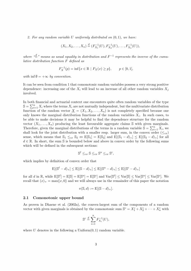
2. For any random variable U uniformly distributed on (0, 1), we have:

(X1, X2, . . . , Xn)d= (F−1

X1(U), F−1

X2(U), . . . , F−1

Xn(U)),

where “d=” means as usual equality in distribution and F−1 represents the inverse of the cumu-

lative distribution function F defined as

F−1X (p) = inf{x ∈ R | FX(x) ≥ p}, p ∈ [0, 1],

with inf ∅ = +∞ by convention.

It can be seen from condition 1 that comonotonic random variables possess a very strong positivedependence: increasing one of the Xi will lead to an increase of all other random variables Xj

involved.

In both financial and actuarial context one encounters quite often random variables of the typeS =

∑ni=1 Xi where the terms Xi are not mutually independent, but the multivariate distribution

function of the random vector X = (X1, X2, . . . , Xn) is not completely specified because oneonly knows the marginal distribution functions of the random variables Xi. In such cases, tobe able to make decisions it may be helpful to find the dependence structure for the randomvector (X1, . . . , Xn) producing the least favourable aggregate claims S with given marginals.Therefore, given the marginal distributions of the terms in a random variable S =

∑ni=1 Xi, we

shall look for the joint distribution with a smaller resp. larger sum, in the convex order (≤cx)sense, which means that S1 ≤cx S2 ⇔ E[S1] = E[S2] and E[(S1 − d)+] ≤ E[(S2 − d)+] for alld ∈ R. In short, the sum S is bounded below and above in convex order by the following sumswhich will be defined in the subsequent sections:

S` ≤cx S ≤cx S

u ≤cx Sc,

which implies by definition of convex order that

E[(S` − d)+] ≤ E[(S − d)+] ≤ E[(Su − d)+] ≤ E[(Sc − d)+]

for all d in R, while E[S`] = E[S] = E[Su] = E[Sc] and Var[S`] ≤ Var[S] ≤ Var[Su] ≤ Var[Sc]. Werecall that (x)+ = max{x, 0} and we will always use in the remainder of this paper the notation

π(S, d) := E[(S − d)+].

2.1 Comonotonic upper bound

As proven in Dhaene et al. (2002a), the convex-largest sum of the components of a randomvector with given marginals is obtained by the comonotonic sum S

c = Xc1 + Xc

2 + · · ·+ Xcn with

Sc d=

n∑

i=1

F−1Xi

(U),

where U denotes in the following a Uniform(0, 1) random variable.

3

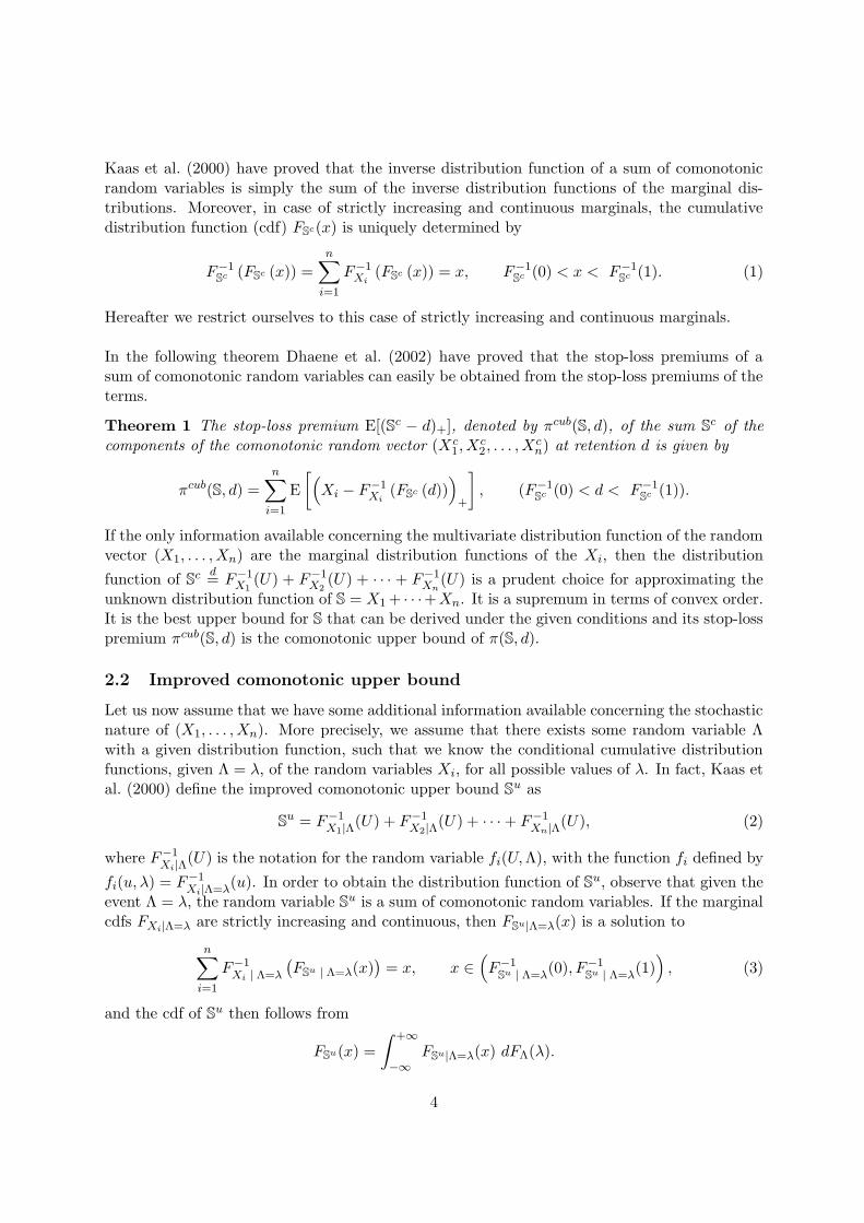
Kaas et al. (2000) have proved that the inverse distribution function of a sum of comonotonicrandom variables is simply the sum of the inverse distribution functions of the marginal dis-tributions. Moreover, in case of strictly increasing and continuous marginals, the cumulativedistribution function (cdf) FSc(x) is uniquely determined by

F−1Sc (FSc (x)) =

n∑

i=1

F−1Xi

(FSc (x)) = x, F−1Sc (0) < x < F−1

Sc (1). (1)

Hereafter we restrict ourselves to this case of strictly increasing and continuous marginals.

In the following theorem Dhaene et al. (2002) have proved that the stop-loss premiums of asum of comonotonic random variables can easily be obtained from the stop-loss premiums of theterms.

Theorem 1 The stop-loss premium E[(Sc − d)+], denoted by πcub(S, d), of the sum Sc of the

components of the comonotonic random vector (Xc1, X

c2, . . . , X

cn) at retention d is given by

πcub(S, d) =n∑

i=1

E

[

(

Xi − F−1Xi

(FSc (d)))

+

]

, (F−1Sc (0) < d < F−1

Sc (1)).

If the only information available concerning the multivariate distribution function of the randomvector (X1, . . . , Xn) are the marginal distribution functions of the Xi, then the distribution

function of Sc d

= F−1X1

(U) + F−1X2

(U) + · · · + F−1Xn

(U) is a prudent choice for approximating theunknown distribution function of S = X1 + · · ·+Xn. It is a supremum in terms of convex order.It is the best upper bound for S that can be derived under the given conditions and its stop-losspremium πcub(S, d) is the comonotonic upper bound of π(S, d).

2.2 Improved comonotonic upper bound

Let us now assume that we have some additional information available concerning the stochasticnature of (X1, . . . , Xn). More precisely, we assume that there exists some random variable Λwith a given distribution function, such that we know the conditional cumulative distributionfunctions, given Λ = λ, of the random variables Xi, for all possible values of λ. In fact, Kaas etal. (2000) define the improved comonotonic upper bound S

u as

Su = F−1

X1|Λ(U) + F−1

X2|Λ(U) + · · · + F−1

Xn|Λ(U), (2)

where F−1Xi|Λ

(U) is the notation for the random variable fi(U, Λ), with the function fi defined by

fi(u, λ) = F−1Xi|Λ=λ(u). In order to obtain the distribution function of S

u, observe that given theevent Λ = λ, the random variable S

u is a sum of comonotonic random variables. If the marginalcdfs FXi|Λ=λ are strictly increasing and continuous, then FSu|Λ=λ(x) is a solution to

n∑

i=1

F−1Xi | Λ=λ

(

FSu | Λ=λ(x))

= x, x ∈(

F−1Su | Λ=λ(0), F−1

Su | Λ=λ(1))

, (3)

and the cdf of Su then follows from

FSu(x) =

∫ +∞

−∞FSu|Λ=λ(x) dFΛ(λ).

4

In this case, we also find that for any d ∈(

F−1Su|Λ=λ(0), F−1

Su|Λ=λ(1))

:

E[

(Su − d)+ | Λ = λ]

=n∑

i=1

E

[

(

Xi − F−1Xi|Λ=λ

(

FSu|Λ=λ(d))

)

+| Λ = λ

]

.

Integration with respect to λ over the real line leads to the improved comonotonic upper bound,denoted by πicub(S, d, Λ), for π(S, d).

Theorem 2 The stop-loss premium E[(Su − d)+] of the improved comonotonic upper bound Su

for S at retention d is given by

πicub(S, d, Λ) =

∫ +∞

−∞

n∑

i=1

E

[

(

Xi − F−1Xi|Λ=λ

(

FSu|Λ=λ(d))

)

+| Λ = λ

]

dFΛ(λ),

(

F−1Su|Λ=λ (0) < d < F−1

Su|Λ=λ (1))

with Λ the conditioning variable in definition (2) of Su and where FSu|Λ=λ(d) can be obtained

from (3).

2.3 Lower bound

Let X = (X1, . . . , Xn) be a random vector with given marginal cdfs FX1 , FX2 , . . . , FXn . Assumeagain that there exists some random variable Λ with a given distribution function, such thatwe know the conditional distribution, given Λ = λ, of the random variables Xi, for all possiblevalues of λ. We recall from Kaas et al. (2000) that a lower bound, in the sense of convex order,for S = X1 + X2 + · · · + Xn is

S` = E [S | Λ] . (4)

This idea can also be found in Rogers and Shi (1995) for the continuous case.

Let us further assume that the random variable Λ is such that all E [Xi | Λ] are non-decreasingand continuous functions of Λ, then according to the first condition of Properties 1 S

` is acomonotonic sum. When in addition the cdfs of the random variables E [Xi | Λ] are strictlyincreasing and continuous, then the cdf of S

` is also strictly increasing and continuous, and weget analogously to (1) for all x ∈

(

F−1S` (0) , F−1

S` (1))

,

F−1S` (FS`(x)) =

n∑

i=1

F−1E[Xi|Λ] (FS`(x)) = x, (5)

which unambiguously determines the cdf of the convex order lower bound S` for S. Using the

fact that for a non-decreasing continuous function g, we have

F−1g(X)(p) = g(F−1

X (p)), p ∈ (0, 1),

and relation (5) is equivalent to

n∑

i=1

E[

Xi | Λ = F−1Λ (FS`(x))

]

= x. (6)

Invoking Theorem 1, the stop-loss premium E[(S` − d)+], denoted by π`b(S, d, Λ), of the lowerbound S

`, is obtained:

5

Theorem 3 The stop-loss premium of the lower bound S` for S at retention d is given by

π`b(S, d, Λ) =n∑

i=1

E[

(

E [Xi | Λ] − E[

Xi | Λ = F−1Λ (FS`(d))

])

+

]

,(

F−1S` (0) < d < F−1

S` (1))

(7)with Λ the conditioning variable in definition (4) of S

` and where FS`(d) can be obtained from(5).

Remark 1

1. So far, we considered the case that all E [Xi | Λ] are non-decreasing functions of Λ. Thecase where all E [Xi | Λ] are non-increasing and continuous functions of Λ also leads to acomonotonic vector (E [X1 | Λ] , E [X2 | Λ] , . . . , E [Xn | Λ]), and can be treated in a similarway but will not be dealt with in this paper.

2. In case the cdfs of the random variables E [Xi | Λ] are not continuous nor strictly increasingor decreasing functions of Λ, then the stop-loss premiums of S

`, which is not comonotonicanymore, can be determined as follows :

π`b(S, d, Λ) =

∫ +∞

−∞

(

n∑

i=1

E [Xi | Λ = λ] − d

)

+

dFΛ (λ) . (8)

3 Upper bounds based on lower bound plus error term

Following the ideas of Rogers and Shi (1995) and analogous to Vanmaele et al. (2006), we derivean upper bound based on the lower bound.

Theorem 4 The upper bound πeub(S, d, Λ) for the stop-loss premium π(S, d) with retention d isgiven by

πeub(S, d, Λ) = π`b(S, d, Λ) + ε,

where the error bound ε equals

ε :=1

2E

n∑

i=1

n∑

j=1

E [XiXj | Λ] −(

S`)2

1/2

, (9)

and with Λ the conditioning variable in definition (4) of S`.

Proof:Indeed, applying the following general inequality for any random variable Y and Z from Rogersand Shi (1995):

0 ≤ E[

E [Y+ | Z] − E [Y | Z]+]

≤ 1

2E[

√

Var(Y | Z)]

(10)

to the case of Y being S− d and Z being our conditioning variable Λ, we obtain an error bound

0 ≤ E[

E [(S − d)+ | Λ] − (S` − d)+

]

≤ 1

2E[

√

Var(S | Λ)]

:= ε, (11)

6

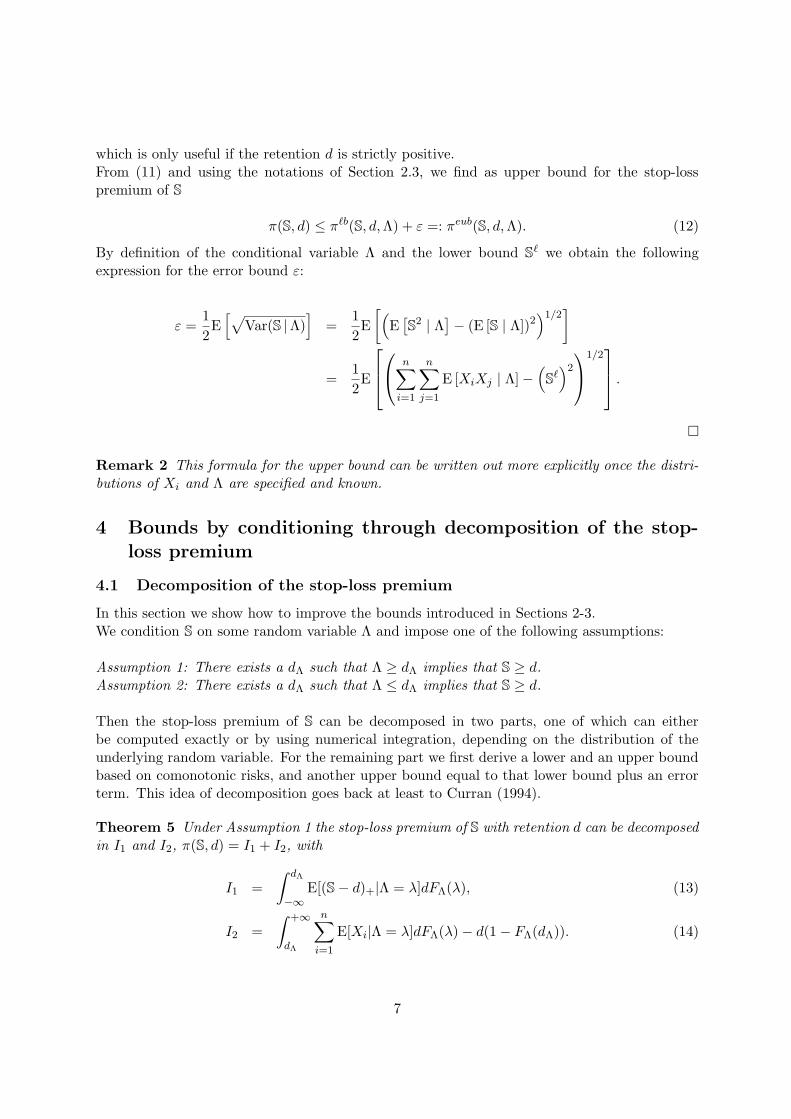
which is only useful if the retention d is strictly positive.From (11) and using the notations of Section 2.3, we find as upper bound for the stop-losspremium of S

π(S, d) ≤ π`b(S, d, Λ) + ε =: πeub(S, d, Λ). (12)

By definition of the conditional variable Λ and the lower bound S` we obtain the following

expression for the error bound ε:

ε =1

2E[

√

Var(S |Λ)]

=1

2E

[

(

E[

S2 | Λ

]

− (E [S | Λ])2)1/2

]

=1

2E

n∑

i=1

n∑

j=1

E [XiXj | Λ] −(

S`)2

1/2

.

�

Remark 2 This formula for the upper bound can be written out more explicitly once the distri-butions of Xi and Λ are specified and known.

4 Bounds by conditioning through decomposition of the stop-

loss premium

4.1 Decomposition of the stop-loss premium

In this section we show how to improve the bounds introduced in Sections 2-3.We condition S on some random variable Λ and impose one of the following assumptions:

Assumption 1: There exists a dΛ such that Λ ≥ dΛ implies that S ≥ d.Assumption 2: There exists a dΛ such that Λ ≤ dΛ implies that S ≥ d.

Then the stop-loss premium of S can be decomposed in two parts, one of which can eitherbe computed exactly or by using numerical integration, depending on the distribution of theunderlying random variable. For the remaining part we first derive a lower and an upper boundbased on comonotonic risks, and another upper bound equal to that lower bound plus an errorterm. This idea of decomposition goes back at least to Curran (1994).

Theorem 5 Under Assumption 1 the stop-loss premium of S with retention d can be decomposedin I1 and I2, π(S, d) = I1 + I2, with

I1 =

∫ dΛ

−∞E[(S − d)+|Λ = λ]dFΛ(λ), (13)

I2 =

∫ +∞

dΛ

n∑

i=1

E[Xi|Λ = λ]dFΛ(λ) − d(1 − FΛ(dΛ)). (14)

7

Proof:

By the tower property for conditional expectations the stop-loss premium π(S, d) with S =n∑

i=1Xi

equalsE[E[(S − d)+|Λ]],

for some conditioning variable Λ with cdf FΛ.By Assumption 1 it holds that on the set {Λ ≥ dΛ}

E[(S − d)+ | Λ] = E[S − d | Λ](4)= (S` − d)+,

which immediately leads to:

π(S, d) =

∫ dΛ

−∞E[(S − d)+|Λ = λ]dFΛ(λ) +

∫ +∞

dΛ

E[S − d|Λ = λ]dFΛ(λ). (15)

The expression (14) for the second integral I2 in the decomposition of the stop-loss premium ofS is a straightforward simplification of the second integral in (15).

�

Remark 3

1. Under Assumption 2 a similar decomposition holds with the appropriate integration bounds.

2. In practical applications the existence of such a dΛ depends on the actual form of S and Λ.

3. The second integral I2 can be written out explicitly if the bivariate distribution of (Xi, Λ)is known for all i.

In the following three subsections we derive bounds for the first integral I1 in (13) and add themup to the exact part (14) in order to obtain bounds for the stop-loss premium π(S, d) itself.

4.2 Lower bound

By means of Jensen’s inequality, the first integral I1 in (13) can be bounded below:

I1 ≥∫ dΛ

−∞(E[S | Λ = λ] − d)+dFΛ(λ) =

∫ dΛ

−∞

(

n∑

i=1

E[Xi|Λ = λ] − d)

+dFΛ(λ). (16)

By adding the exact part (14) and using the notations of Section 2.3, we end up with theinequality of Section 2.3:

π(S, d) ≥ π`b(S, d, Λ).

Thus, when S` is a sum of n comonotonic risks we can apply (7) which holds even when we do

not know or find an appropriate dΛ.

When S` is not comonotonic we use under Assumption 1 the decomposition

π`b(S, d, Λ) =

∫ dΛ

−∞(

n∑

i=1

E[Xi|Λ = λ]−d)+dFΛ(λ)+

∫ +∞

dΛ

n∑

i=1

E[Xi|Λ = λ]dFΛ(λ)−d(1−FΛ(dΛ)),

instead of formula (8).

8

4.3 Upper bound based on lower bound

Under Assumption 1 we improve the bound (12) by making the error bound ε (9) dependent onthe integration bound dΛ.

Theorem 6 Under Assumption 1 the upper bound πdeub for the stop-loss premium π(S, d) withretention d is given by

πdeub(S, d, Λ) = π`b(S, d, Λ) + ε(dΛ), (17)

where the error bound ε(dΛ) equals

ε(dΛ) :=1

2

(

E[

Var (S | Λ) 1{Λ<dΛ}

]) 12(

E[

1{Λ<dΛ}

]) 12 , (18)

where 1{Λ<dΛ} is the indicator function, i.e. 1{c} = 1 if the condition c is true and 1{c} = 0 if itis not.

Proof:By applying inequality (10) to (16) and using Holder’s inequality we find that

0 ≤ E[

E[(S − d)+ | Λ] − (S` − d)+

]

=

∫ dΛ

−∞

(

E[(S − d)+ | Λ = λ] − (E [ S | Λ = λ] − d)+)

dFΛ(λ)

≤ 1

2

∫ dΛ

−∞(Var (S | Λ = λ))

12 dFΛ(λ) (19)

≤ 1

2

(

E[

Var (S | Λ) 1{Λ<dΛ}

]) 12(

E[

1{Λ<dΛ}

]) 12 .

�

Remark 4 The error bound (9), and hence also the upper bound πeub(S, d, Λ), is independentof dΛ and corresponds to the limiting case of (19) where dΛ equals infinity. Obviously, the errorbound (19) improves the error bound (9). In practical applications, the additional error intro-

duced by Holders inequality turns out to be much smaller than the difference 12E[

√

Var(S|Λ)]

−ε(dΛ).

4.4 Partially exact/comonotonic upper bound

Under Assumption 1 another upper bound can be obtained. Hereto we bound the first term I1

in (13) by replacing S | Λ = λ by its comonotonic upper bound Su (in convex order sense):

∫ dΛ

−∞E[(S − d)+ | Λ = λ]dFΛ(λ) ≤

∫ dΛ

−∞E[(Su − d)+ | Λ = λ]dFΛ(λ). (20)

Adding (20) to the exact part (14) of the decomposition of the stop-loss premium of S resultsin the so-called partially exact/comonotonic upper bound for a stop-loss premium. We will usethe notation πpecub(S, d, Λ) to indicate this upper bound.

9

Theorem 7 Under Assumption 1 the partially exact/comonotonic upper bound for π(S, d) isgiven by

πpecub(S, d, Λ) =

∫ dΛ

−∞E[(Su−d)+ | Λ = λ]dFΛ(λ)+

∫ +∞

dΛ

n∑

i=1

E[Xi|Λ = λ]dFΛ(λ)−d(1−FΛ(dΛ)).

(21)

Remark 5 It is easily seen that

πpecub(S, d, Λ) ≤ πicub(S, d, Λ),

while for two distinct conditioning variables Λ1 and Λ2 it does not necessarily holds that

πpecub(S, d, Λ1) ≤ πicub(S, d, Λ2).

4.5 Compounded sums

In this subsection we study compounded sums of the following form

SN =

N∑

i=1

Xi, (22)

with N a stochastic number which is independent of (Xi)i.

Theorem 8 The stop-loss premium E[(SN −d)+], denoted by π(SN , d), of the compounded sumSN at retention d is given by

π(SN , d) =∞∑

j=1

Pr(N = j) π(Sj , d), (23)

with

Sj =

j∑

i=1

Xi.

Proof:Using the tower property for conditional expectations, we can calculate the stop-loss premiumof SN as follows

π(SN , d) = E[

(SN − d)+]

= E

(

N∑

i=1

Xi − d

)

+

= EN

E

(

N∑

i=1

Xi − d

)

+

|N

=

∞∑

j=1

Pr(N = j)E

(

j∑

i=1

Xi − d

)

+

=∞∑

j=1

Pr(N = j) π

(

j∑

i=1

Xi, d

)

.

10

�

Remark that in practical applications the infinite time horizon is often replaced by a finitenumber.

It is straightforward to obtain a lower bound, denoted as π`b(SN , d,Λ), by looking at the com-bination

π`b(SN , d,Λ) =∞∑

j=1

Pr(N = j) π`b(Sj , d, Λj),

with Λ = Λ1, Λ2, . . . and π`b(Sj , d, Λj) given by (7) for n = j. The same reasoning can befollowed for obtaining the comonotonic upper bound πcub(SN , d), the improved comonotonicupper bound πicub(SN , d,Λ) and the partially exact/comonotonic upper bound πpecub(SN , d,Λ).

For each term π(Sj , d) in the sum (23) we can take the minimum of two or more of the abovedefined upper bounds. We propose two upper bounds based on this simple idea.

The first bound takes each time the minimum of the error term (9) independent of the retentionand the error term (18) dependent on the retention. Combining this with the stop-loss premiumof the lower bound S

` results in the following upper bound

πemub(SN , d,Λ) = π`b(SN , d,Λ) +∞∑

j=1

Pr(N = j) min

(

1

2E

[

√

Var[Sj |Λj ]

]

, ε(dΛj)

)

.

Calculating for each term the minimum of all the presented upper bounds

πmin(SN , d,Λ) =∞∑

j=1

Pr(N = j) min(

πcub(Sj , d), πicub(Sj , d, Λj), πpecub(Sj , d, Λj), π

emub(Sj , d, Λj))

,

will of course provide the best possible upper bound.Remark that πemub(Sj , d, Λj) = π`b(Sj , d, Λj) + min

(

12E[√

Var[Sj |Λj ]]

, ε(dΛj))

.

5 Case of sum of lognormal random variables

In this section we further develop the expressions for the lower and upper bounds when therandom variables Xi in the sum S are lognormal.

We assume that Xi = αieZi with Zi ∼ N(E[Zi], σZi

) and αi ∈ R, i.e.

S =n∑

i=1

Xi =n∑

i=1

αieZi . (24)

In this case the stop-loss premium with some retention di, namely π(Xi, di), is well-known fromthe following lemma.

11

Lemma 1 Let X be a lognormal random variable of the form αeZ with Z ∼ N(E[Z], σZ) andα ∈ R. Then the stop-loss premium with retention d equals for αd > 0

π(X, d) = sign (α) eµ+σ2

2 Φ(sign (α) b1) − dΦ(sign (α) b2), (25)

where

µ = ln |α| + E[Z] σ = σZ

b1 =µ + σ2 − ln |d|

σb2 = b1 − σ (26)

and where Φ stands for the cdf of a standard normal random variable. The case αd < 0 is trivial.

We now consider a normally distributed random variable Λ. The following results are analogousto Theorem 1 in Dhaene et al. (2002b).

Theorem 9 Let S be given by (24) and consider a normally distributed random variable Λ whichis such that (Zi, Λ) is bivariate normally distributed for all i. Then the distributions of the lowerbound S

`, the improved comonotonic upper bound Su and the comonotonic upper bound S

c aregiven by

S` =

n∑

i=1

αieE[Zi]+riσZi

Φ−1(V )+ 12(1−r2

i )σ2Zi , (27)

Su =

n∑

i=1

αieE[Zi]+riσZi

Φ−1(V )+sign(αi)√

1−r2i σZi

Φ−1(U), (28)

Sc =

n∑

i=1

αieE[Zi]+sign(αi)σZi

Φ−1(U), (29)

where U and V = Φ

(

Λ − E[Λ]

σΛ

)

are mutually independent Uniform(0,1) random variables, Φ

is the cdf of the N(0, 1) distribution and ri, i = 1, . . . , n, are correlations defined by

ri = r (Zi, Λ) =Cov [Zi, Λ]

σZiσΛ

.

When for all i sign(αi) = sign(ri) or for all i sign(αi) = −sign(ri) for ri 6= 0 then S` is

comonotonic.

5.1 Comonotonic upper bound

Since the cdfs FXiare strictly increasing and continuous, it follows from (1) and (29) that for

x ∈(

F−1Sc (0), F−1

Sc (1))

, the cdf of the comonotonic sum FSc(x) can be found by solving

n∑

i=1

αieE[Zi]+sign(αi)σZi

Φ−1(FSc (x)) = x.

Combination of Theorem 1 and Lemma 1 yields the following expression for the stop-loss pre-mium of S

c at retention d with F−1Sc (0) < d < F−1

Sc (1):

πcub(S, d) =n∑

i=1

αieE[Zi]+

σ2Zi2 Φ

[

sign(αi)σZi− Φ−1(FSc(d))

]

− d (1 − FSc(d)) .

12

5.2 Improved comonotonic upper bound

We now determine the cdf of Su and the stop-loss premium πicub(S, d, Λ), where we condition on

a normally distributed random variable Λ or equivalently on the Uniform(0, 1) random variableintroduced in Theorem 9:

V = Φ

(

Λ − E [Λ]

σΛ

)

.

The conditional probability FSu|V =v(x) also denoted by FSu(x | V = v), is the cdf of a sum of

n comonotonic random variables and follows for F−1Su|V =v(0) < x < F−1

Su|V =v(1), according to (3)

and (28), implicitly from:

n∑

i=1

αieE[Zi]+riσZi

Φ−1(v)+sign(αi)√

1−r2i σZi

Φ−1(FSu (x|V =v)) = x. (30)

The cdf of Su is then given by

FSu(x) =

∫ 1

0FSu|V =v(x)dv.

We now look for an expression for the stop-loss premium for Su at retention d with F−1

Su|V =v(0) <

d < F−1Su|V =v(1):

πicub(S, d, Λ) =

∫ 1

0E[

(Su − d)+ | V = v]

dv =n∑

i=1

∫ 1

0E

[

(

F−1Xi|Λ

(U | V = v) − di

)

+

]

dv

with di = F−1Xi|Λ

(FSu(d | V = v) | V = v) and with U a random variable which is uniformly

distributed on (0, 1). Since sign(αi)F−1Xi|Λ

(U | V = v) follows a lognormal distribution withmean and standard deviation:

µv(i) = ln |αi| + E [Zi] + riσZiΦ−1(v), σv(i) =

√

1 − r2i σZi

,

one obtains that

di = αi exp

[

E [Zi] + riσZiΦ−1(v) + sign(αi)

√

1 − r2i σZi

Φ−1(

FSu|V =v(d))

]

.

The well-known formula (25) then yields

E[

(Su − d)+ | V = v]

=

n∑

i=1

[

sign(αi)eµv(i)+

σ2v(i)

2 Φ(sign(αi)bi,1) − diΦ(sign(αi)bi,2)

]

,

with, according to (26),

bi,1 =µv(i) + σ2

v(i) − ln |di|σv(i)

, bi,2 = bi,1 − σv(i).

Substitution of the corresponding expressions and integration over the interval [0, 1] leads underthe assumptions of Theorems 2 and 9 to the following result

πicub(S, d, Λ) =n∑

i=1

αieE[Zi]+

12σ2

Zi(1−r2

i )∫ 1

0eriσZi

Φ−1(v)×

× Φ

(

sign(αi)√

1 − r2i σZi

− Φ−1(

FSu|V =v(d))

)

dv − d (1 − FSu(d)) . (31)

13

5.3 Lower bound

In this subsection and under the assumptions of Theorems 3 and 9, we study the case that, forall i, sign(αi) = sign(ri) when ri 6= 0. For simplicity we take all αi ≥ 0 and assume that theconditioning variable Λ is normally distributed and has the right sign such that the correlationcoefficients ri are all positive. According to property 1 of Properties 1 these conditions ensurethat S

` is the sum of n comonotonic random variables. The case that, for all i, sign(αi) =−sign(ri) when ri 6= 0 can be dealt with in an analogous way.

Since by our assumptions E[Xi | Λ] is increasing, we can obtain FS`(x) according to (5) and (27)from

n∑

i=1

αieE[Zi]+riσZi

Φ−1(FS` (x))+ 1

2(1−r2i )σ2

Zi = x. (32)

Moreover as S` is the sum of n lognormally distributed random variables, the stop-loss premium

at retention d(> 0) can be expressed explicitly by invoking Theorem 1 and Lemma 1:

π`b(S, d, Λ) =n∑

i=1

αieE[Zi]+

12σ2

Zi Φ[

riσZi− Φ−1 (FS`(d))

]

− d (1 − FS`(d)) . (33)

5.4 Upper bound based on lower bound

From (9) we obtain that

E[

√

Var(S |Λ)]

=

∫ +∞

−∞

n∑

i=1

n∑

j=1

E [XiXj | Λ = λ] − (E[S | Λ = λ])2

12

dFΛ(λ). (34)

Now consider the first term in the right hand side of (34). According to the properties oflognormally distributed random variables, the product of lognormals is again lognormal, andconditioning a lognormal variate on a normal variate yields a lognormally distributed variable.

We can proceed by denoting Zij = Zi + Zj with E[Zij ] = E[Zi] + E[Zj ] and

σ2Zij

= σ2Zi

+ σ2Zj

+ 2σZiZj,

where σZiZjstands for Cov(Zi, Zj). Note that

rij =Cov(Zij , Λ)

σZijσΛ

=Cov (Zi, Λ)

σZijσΛ

+Cov (Zj , Λ)

σZijσΛ

=σZi

σZij

ri +σZj

σZij

rj .

Conditionally, given Λ = λ, the random variable Zij is normally distributed with parameters

µ(ij) = E [Zij ] + rijσZij

σΛ(λ − E [Λ]) and σ2(ij) =

(

1 − r2ij

)

σ2Zij

. Hence, conditionally, given

14

Λ = λ, the random variable eZij is lognormally distributed with parameters µ(ij) and σ2(ij).

As E[

eZij | Λ = λ]

= eµ(ij)+ 12σ2(ij), we find

E[

eZij | Λ]

= eE[Zij ]+rijσZij

Φ−1(V )+ 12(1−r2

ij)σ2Zij ,

where the random variable V = Φ(

Λ−E[Λ]σΛ

)

is uniformly distributed on the interval (0, 1).

Thus, the first term in (34) equals

n∑

i=1

n∑

j=1

E[XiXj | Λ] =n∑

i=1

n∑

j=1

αiαj exp

(

E[Zij ] + rijσZijΦ−1(V ) +

1

2(1 − r2

ij)σ2Zij

)

, (35)

while the second term consists of (27). Hence (34) can be written out explicitly and we havethat the upper bound (12) is given by

πeub(S, d, Λ) =n∑

i=1

αieE[Zi]+

12σ2

Zi Φ[

riσZi− Φ−1 (FS`(d))

]

− d (1 − FS`(d)) +

+1

2

∫ 1

0

{

n∑

i=1

n∑

j=1

αiαjeE[Zij ]+rijσZij

Φ−1(v)+ 12(1−r2

ij)σ2Zij−

−(

n∑

i=1

αieE[Zi]+riσZi

Φ−1(v)+ 12(1−r2

i )σ2Zi

)2 } 12

dv.

5.5 Bounds by conditioning through decomposition of stop-loss premium

In this subsection we apply the theory of Section 4 to the sum of lognormal random variables(23). We only give here the analytical expressions for the two upper bounds πdeub(S, d, Λ) andπpecub(S, d, Λ). For more details concerning the calculation of the bounds the reader is referredto Appendix A and B.

The following auxiliary result is needed in order to write out the bounds explicitely.

Lemma 2 For any constant a ∈ R and any normally distributed random variable Λ

∫ dΛ

−∞eaΦ−1(v)dFΛ(λ) = e

a2

2 Φ(d∗Λ − a), (36)

where d∗Λ = dΛ−E[Λ]σΛ

, V = Φ(

Λ−E[Λ]σΛ

)

is uniformly distributed on the unit interval and thus,

Φ−1(V ) = Λ−E[Λ]σΛ

is a standard normal variable.

5.5.1 Lower bound

In view of the remark that the lower bound via the decomposition equals the lower boundwithout the decomposition, we refer for an expression for it in the lognormal and comonotoniccase to Section 5.3.

15

5.5.2 Upper bound based on lower bound

Under the assumptions of Theorems 6 and 9 the upper bound (17) can be written out explicitlyas follows

πdeub(S, d, Λ) =n∑

i=1

αieE[Zi]+

12σ2

Zi Φ[

riσZi− Φ−1 (FS`(d))

]

− d (1 − FS`(d)) +

+1

2Φ(d∗Λ)1/2

{

n∑

i=1

n∑

j=1

αiαjeE[Zi]+sE[Zj ]+

12(σ2

Zi+σ2

Zj)×

×Φ(

d∗Λ −(

riσZi+ rjσZj

)) (

eσZiZj − e

σZiσZj

rirj)

} 12

,

with d∗Λ as in Lemma 2 and where FS`(d) can be obtained from (32).

5.5.3 Partially exact/comonotonic upper bound

Under the assumptions of Theorems 7 and 9 the partially exact/comonotonic upper bound ofsubsection 4.4 is given by

πpecub(S, d, Λ) =n∑

i=1

αieE[Zi]+

12σ2

Zi(1−r2

i ){

e12r2i σ2

Zi Φ(riσZi− d∗Λ) +

∫ Φ(d∗Λ)

0eriσZi

Φ−1(v)×

× Φ

(

sign(αi)√

1 − r2i σZi

− Φ−1(

FSu|V =v(d))

)

dv

}

−

−d

(

1 −∫ Φ(d∗Λ)

0FSu|V =v(d)dv

)

,

with d∗Λ as in Lemma 2 and where FSu|V =v(d) can be obtained from (30).

5.6 Choice of the conditioning variable

If X ≤cx Y , and X and Y are not equal in distribution, then Var[X] < Var[Y ] must hold. An

equality in variance would imply that Xd= Y . This shows that if we want to replace S by the less

convex S`, the best approximations will occur when the variance of S

` is ‘as close as possible’to the variance of S. Hence we should choose Λ such that goodness-of-fit expressed by the ratio

z = Var(S`)

Var(S)is as close as possible to 1. Of course one can always use numerical procedures to

optimize z but this would outweigh one of the main features of the convex bounds, namely thatthe different relevant actuarial quantities (quantiles, tailvars, stop-loss premiums) can be easilyobtained. Having a ready-to-use approximation that can be easily implemented and used by allkind of end-users is important from a business point of view.

We propose here three conditioning random variables. The first two are linear combinations ofthe random variables Zi:

Λ =

n∑

i=1

γi Zi, (37)

16

for particular choices of the coefficients γi.

Kaas, Dhaene and Goovaerts (2000) propose a first choice for the parameters γi when computingthe lower bound S

`:γi = αie

E[Zi], i = 1, . . . , n. (38)

This ‘Taylor-based’ choice makes Λ a linear transformation of a first order approximation to S.This can be seen from the following derivation:

S =n∑

i=1

αieE[Zi] +(Zi−E[Zi]) ≈

n∑

i=1

αieE[Zi] (1 + Zi − E [Zi])

≈ C +n∑

i=1

αieE[Zi]Zi, (39)

where C is the appropriate constant. Hence S` will be “close” to S, provided (Zi − E(Zi)) is

sufficiently small, or equivalently, σ2Zi

is sufficiently small. One intuitively expects that for this

choice for Λ, E(Var[S | Λ]) is “small” and since Var(S) = E(Var[S | Λ]) + Var(S`) this exactly

means that one expects the ratio z = Var(S`)

Var(S)to tend to one.

A possible decomposition variable is in that case given by

dΛ = d − C = d −n∑

i=1

αieE[Zi] (1 − E [Zi]) . (40)

Using the property that ex ≥ 1 + x and (39), we have that Λ ≥ dΛ implies that S ≥ d.

A second conditioning variable is proposed by Vanduffel, Hoedemakers and Dhaene (2004) forwhich the first order approximation of Var(S`) is maximized. They take in expression (37) forΛ the parameters γi equal to

γi = αieE[Zi]+

12σ2

Zi , i = 1, . . . , n. (41)

For this ‘maximal variance’ conditioning variable a possible choice for dΛ is given by

dΛ = d −n∑

i=1

αieE[Zi]+

12σ2

Zi

(

1 − E [Zi] −1

2σ2

Zi

)

. (42)

A third conditioning variable is based on the standardized logarithm of the geometric averageG = (

∏ni=1 S)1/n as in Nielsen and Sandman (2002)

Λ =ln G − E[ln G]√

Var(ln G)=

∑ni=1(Zi − E[Zi])√

Var(∑n

i=1 Zi).

Using the fact that the geometric average is not greater than the arithmetic average, a possibledecomposition variable is here given by

dΛ =n ln

(

dn

)

−∑ni=1 E[Zi]

√

Var(∑n

i=1 Zi),

17

so that Λ ≥ dΛ implies that S ≥ d.

In the remainder of this paper, the choice of Λ will be dependent on the time horizon n. Toindicate this dependence, we introduce the notation Λn for the used conditioning variable Λ.

5.7 Generalization to sums of lognormals with a stochastic time horizon

Suppose that S is a sum of lognormal variables with a stochastic time horizon T

ST =

T∑

i=1

αieZi ,

with αi ∈ R, T a stochastic variable with life time probability distribution FT (t) and Zi ∼N(E[Zi], σZi

) independent of T . Using Theorem 8 the stop-loss premium of ST can be writtendown as follows

π(ST , d) = E[

(ST − d)+]

=

∞∑

j=1

Pr(T = j) π(Sj , d),

with

Sj =

j∑

i=1

αieZi .

6 Applications and numerical illustrations

6.1 Life contingencies

In the first part of this section, we will adapt the different lower and upper bounds presentedabove, to the case of life contingencies, and we will compare the performance in a numericalillustration. We consider the random variable Sn which is defined as the present value of aseries of n deterministic non-negative payment obligations α1, α2, . . . , αn due at times 1, 2, . . . , n,respectively:

Sn =n∑

i=1

αie−Y (i) :=

n∑

i=1

αieZi , (43)

where the stochastic variables Y (i) are defined as Y (i) := Y1+Y2+· · ·+Yi. The random variablesYi represent the stochastic continuous compounded rate of return over the period [i − 1, i] ande−Y (i) is the random discount factor over the period [0, i].

We will assume that the yearly returns Yi are i.i.d. normally distributed with mean µ = 0.07and volatility σ = 0.1. Notice that Sn is a random variable of the general type defined in (24).

In order to compute the lower and upper bounds for the stop-loss premia, we consider as condi-tioning random variable Λn =

∑ni=1 γi Zi, with in the ‘Taylor-based’ case γi given by (38) and

in the ‘maximal variance’ case γi given by (41). The corresponding decomposition variables arerespectively equal to (40) and (42). For the numerical illustrations in this section we presenteach time the one which provides the best result.

18

Notice that E[Zi], σ2Zi

and ri are given by

E[Zi] = −iµ,

σ2Zi

= iσ2

and

ri =

∑ij=1

∑nk=j γk

√

i∑n

j=1

(

∑nk=j γk

)2.

Remark that the correlation coefficients ri are positive, so that the formulae (32) and (33) canbe applied.

The ‘maximal variance’ conditioning variable (41) performs better far in the tail. So for highvalues of d the different bounds based on this conditioning variable approximate more accuratethe real value of the stop-loss premium than the approximations using the ‘Taylor-based’ condi-tioning variable (38). The ‘geometric average’ conditioning variable performs in general sligthlyworse in comparison with the two other random variables for this kind of applications.

Now we will compare the performance of the different bounds that were presented in Sections 2, 3and 4: the lower bound π`b(Sn, d, Λ) (LB), the comonotonic upper bound πcub(Sn, d) (CUB), theimproved comonotonic upper bound πicub(Sn, d, Λ) (ICUB), the upper bound based on the lowerbound πeub(Sn, d, Λ) (EUB) and πdeub(Sn, d, Λ) (DEUB) and the partially exact/comonotonicupper bound πpecub(Sn, d, Λ) (PECUB). For applications with a stochastic time horizon N wealso consider the two combination bounds πemub(SN , d,Λ) (EMUB) and πmin(SN , d,Λ) (MIN).

We will compare the different lower and upper bounds for the stop-loss premiums with thevalues obtained by Monte-Carlo simulation (MC). The simulation results are based on generating50×1 000 000 paths. For each estimate we computed the standard error (s.e.). As is well-known,the (asymptotic) 95% confidence interval is given by the estimate plus or minus 1.96 timesthe standard error. The estimates obtained from this time-consuming simulation will serve asbenchmark. The random paths are based on antithetic variables in order to reduce the varianceof the Monte-Carlo estimates.

We will apply the above derived bounds for two kind of life insurance applications. A life annuitymay be defined as a series of periodic payments where each payment will actually be made onlyif a designated life is alive at the time the payment is due. Let us consider a person aged xyears, also called a life aged x and denoted by (x). We denote his or her future lifetime by Tx.Thus x + Tx will be the age of death of the person. The future lifetime Tx is a random variablewith a probability distribution function

Gx(t) = Pr[Tx ≤ t] = tqx, t ≥ 0.

The function Gx represents the probability that the person will die within t years, for any fixedt. We assume that Gx is known. We define Kx = bTxc, the number of completed future yearslived by (x), or the curtate future lifetime of (x), where b.c is the floor function, i.e. bxc is the

19

largest integer less than or equal to x. The probability distribution of the integer valued randomvariable Kx is given by

Pr(Kx = k) = Pr(k ≤ Tx < k + 1) = k+1qx − kqx = k|qx, k = 0, 1, . . . .

Further, the ultimate age of the life table is denoted by ω, this means that ω − x is the firstremaining lifetime of (x) for which ω−xqx = 1, or equivalently, G−1

x (1) = ω − x.

We assume in this section that the distribution of the remaining lifetime belongs to the Gompertz-Makeham family. Analytic life tables are defined for all ages x ≥ 0. In Makeham’s model1 lx,the number of persons alive at age x, is given by

lx = asxgcx

, (44)

where a > 0, 0 < s < 1, 0 < g < 1 and c > 1. Makeham’s life table results from the force ofmortality function

µξ = α + βcξ, (45)

where α is a constant component, interpreted as capturing accident hazard, and βcξ is a variablecomponent capturing the hazard of aging. The relationship between (44) and (45) is given by

a := l0eβ

log c , s := e−α and g := e− β

log c . (46)

See Bowers et al. (1996) for more details.

For generating one random variate from Makeham’s law, we use the composition method (De-vroye, 1986) and perform the following steps

(a) Generate G from the Gompertz’s law by the well-known inversion method(b) Generate E for the exponential(1) distribution(c) Retain T = min(E/α, G),

where α = − log s, see (46).

In the remainder of this paper, we will always use the standard actuarial notation:

Pr[Tx > t] = tpx, Pr[Tx > 1] = px, Pr[Tx ≤ t] = tqx, Pr[Tx ≤ 1] = qx.

First we consider a whole life annuity on a life (x) which pays an amount of 1 at the end of eachyear, provided the insured is still alive at that time. Assume that the discounting is performed

1we use the Belgian analytic life tables MR and FR for life annuity valuation, with corresponding constantsfor l0, the number of newborns, equal to 1 000 000. For males: a = 1 000 266.63, s = 0.999441703848, g =0.999733441115, c = 1.101077536030, and for females: a = 1 000 048.56, s = 0.999669730966, g = 0.999951440171,c = 1.116792453830.

20

with a random interest rate. The present value at policy issue of the future payments is denoted2

by Spolicyx and equals the sum of the present values of the payments in the respective years:

Spolicyx =

bω−xc∑

i=1

1{Tx>i}e−Y (i) =

Kx∑

i=1

e−Y (i),

where 1{.} denotes the indicator function.

The stop-loss premium for Spolicyx can be calculated as

E

[

(

Spolicyx − d

)

+

]

=

bω−xc∑

i=1

i|qxE

[

(

Si − d)

+

]

,

where Si is a special case of Si defined in (43) for unit payments ((α1, . . . , αi) = (1, . . . , 1)). Wewill approximate E[(Si − d)+] by one of the derived bounds.

Consider a 65-years old male person. The different lower and upper bounds for the stop-losspremium of a whole life annuity due of 1 payable at the end of each year (annuity-immediate)while (65) survives are compared in Table 1. For the retentions d = 5, 10 and 15 the upper

bound πmin(Spolicyx , d,Λ) really improves the comonotonic and improved comonotonic upper

bound. For the extreme cases the values are more or less the same. The lower bound is veryclose to the real stop-loss premium.

d = 0 d = 5 d = 10 d = 15 d = 20 d = 25 d = 30

LB 9.3196 4.6191 1.2269 0.1737 0.0207 0.0026 0.0004MC 9.3196 4.6191 1.2304 0.1739 0.0216 0.0026 0.0004(s.e. × 105) (8.49) (5.48) (0.51) (0.19) (0.01) (0.002)ICUB 9.3196 4.6238 1.3277 0.2530 0.0454 0.0088 0.0019CUB 9.3196 4.6244 1.3389 0.2610 0.0480 0.0095 0.0021EMUB 9.3196 4.6197 1.2400 0.2145 0.0718 0.0545 0.0522PECUB 9.3196 4.6219 1.2839 0.2381 0.0451 0.0088 0.0019MIN 9.3196 4.6195 1.2385 0.2070 0.0444 0.0088 0.0019

Table 1: Approximations for stop-loss premia with retention d of Spolicyx .

In a second application we consider a portfolio of N0 homogeneous life annuity contracts for

which future lifetimes of the insureds T(1)x , T

(2)x , . . . , T

(N0)x are assumed to be independent. Then

the insurer faces two risks: mortality risk and investment risk. Note that from the Law of LargeNumbers the mortality risk decreases with the number of policies N0 while the investmentrisk remains the same (each of the policies is exposed to the same investment risk). Thus for

2in literature denoted by aK , K ≥ 0.

21

sufficiently large N0 the stop-loss premium of the portfolio can be expressed as follows

E

bω−xc∑

i=1

Nie−Y (i) − d

+

= E

N0

bω−xc∑

i=1

Ni

N0e−Y (i) − d

N0

+

≈ N0E

bω−xc∑

i=1

ipxe−Y (i) − d

N0

+

,

where Ni denotes the number of survivals after the i-th year. Hence in the case of large portfoliosof life annuities it suffices to compute stop-loss premiums of an “average” portfolio S

averagex given

by

Saveragex =

bω−xc∑

i=1

ipxe−Y (i),

what has exactly the form of (43) with αi = ipx (i = 1, . . . , bω − xc).

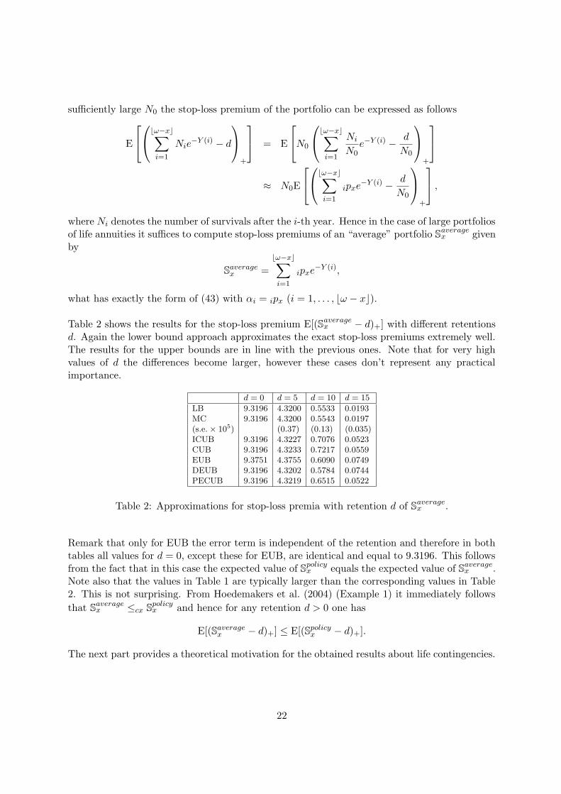
Table 2 shows the results for the stop-loss premium E[(Saveragex − d)+] with different retentions

d. Again the lower bound approach approximates the exact stop-loss premiums extremely well.The results for the upper bounds are in line with the previous ones. Note that for very highvalues of d the differences become larger, however these cases don’t represent any practicalimportance.

d = 0 d = 5 d = 10 d = 15

LB 9.3196 4.3200 0.5533 0.0193MC 9.3196 4.3200 0.5543 0.0197(s.e. × 105) (0.37) (0.13) (0.035)ICUB 9.3196 4.3227 0.7076 0.0523CUB 9.3196 4.3233 0.7217 0.0559EUB 9.3751 4.3755 0.6090 0.0749DEUB 9.3196 4.3202 0.5784 0.0744PECUB 9.3196 4.3219 0.6515 0.0522

Table 2: Approximations for stop-loss premia with retention d of Saveragex .

Remark that only for EUB the error term is independent of the retention and therefore in bothtables all values for d = 0, except these for EUB, are identical and equal to 9.3196. This followsfrom the fact that in this case the expected value of S

policyx equals the expected value of S

averagex .

Note also that the values in Table 1 are typically larger than the corresponding values in Table2. This is not surprising. From Hoedemakers et al. (2004) (Example 1) it immediately follows

that Saveragex ≤cx S

policyx and hence for any retention d > 0 one has

E[(Saveragex − d)+] ≤ E[(Spolicy

x − d)+].

The next part provides a theoretical motivation for the obtained results about life contingencies.

22

6.2 Tail Value-at-Risk

Another application of our results concerns the calculation of Tail Value-at-Risk (TVaR) in asolvency framework. For a given (distribution function of a) random variable S and a givenprobability level p, it is defined by

TVaRp [S] =1

1 − p

∫ 1

pF−1

S(q) dq, 0 < p < 1. (47)

This risk measure is a ‘coherent’ alternative for the ‘Value-at-Risk’ F−1S (p), see e.g. Artzner et

al. (1999). One can prove that TVaRp [X] can also be expressed as

TVaRp [S] = F−1S

(p) +1

1 − pE[

(

S − F−1S

(q))

+

]

, (48)

see e.g. Dhaene et al. (2004). Consider a portfolio consisting of n different business units, eachwith loss Xi and let the sum of the aggregate loss be given by S:

S =n∑

i=1

Xi.

From (47) we see that evaluating TVaRp [S] boils down to evaluating F−1S

(p) and E[

(

S − F−1S

(q))

+

]

.

Let us now assume that the random vector (X1, X2, . . . , Xn) is multivariate lognormal. Accurateapproximations for F−1

S(p) are described in Dhaene et al. (2002a), whereas accurate approxima-

tions for the stop-loss premium E[

(

S − F−1S

(q))

+

]

follow from the results in this paper.

7 Summary and conclusions

In this paper we generalized some methodologies for estimating the stop-loss premiums ofstrongly dependent random variables like the comonotonic approximations of Dhaene et al.(2002a). We started with the upper bound obtained by adding an error term to the lower boundof Rogers and Shi (1995). We explained how these bounds can be improved by decomposing anintegral formula for the stop-loss premium into two parts: one can be easily solved analytically,the other part can be approximated by one of the comonotonic upper bounds. We also studiedbounds for the stop-loss premiums of compounded sums.

We apply all the methods to an average portfolio of life annuities (when mortality risk is assumedto be fully diversified) and to a single life annuity. In the latter case it is possible to decomposethe value of the stop-loss premium by conditioning and apply the best (smallest) upper boundon each of the components separately. We provide a number of numerical illustrations whichshow that the decomposition significantly improves the bounds.

Acknowledgements

Tom Hoedemakers, Grzegorz Darkiewicz and Jan Dhaene acknowledge the financial support ofthe Onderzoeksfonds K.U.Leuven (GOA/02: Actuariele, financiele en statistische aspecten vanafhankelijkheden in verzekerings- en financiele portefeuilles).

23

Michele Vanmaele would like to acknowledge the financial support by the BOF-project 001104599of the Ghent University.Griselda Deelstra acknowledges financial support of the BNB-contract FC0314CR3210.

Corresponding author

Tom HoedemakersCatholic University of LeuvenDepartment of Applied EconomicsNaamsestraat 69, B-3000 Leuven, Belgiumtel: ++32 16 32.67.61, fax: ++32 16 32.67.32email: tom.hoedemakers@econ.kuleuven.be

24

Appendix

A - Upper bound based on lower bound

In the following we shall derive an easily computable expression for (18) in the case of a sum oflognormal random variables.

The second expectation term in the product (18) equals, when denoting by FΛ(·) the normalcumulative distribution function of Λ and by d∗Λ the expression (dΛ − E[Λ])/σΛ,

E[1{Λ<dΛ}] = 0 · P (Λ ≥ dΛ) + 1 · P (Λ < dΛ) = FΛ(dΛ) = Φ(d∗Λ). (49)

The first expectation term in the product (18) can be expressed as

E[

Var (S|Λ) 1{Λ<dΛ}

]

= E[

E[S2|Λ]1{Λ<dΛ}

]

− E[

(E[S|Λ])21{Λ<dΛ}

]

. (50)

Now consider the second term of the right-hand side of (50)

E[

(E[S|Λ])21{Λ<dΛ}

]

=

∫ dΛ

−∞(E[S|Λ = λ])2dFΛ(λ). (51)

According to (27) and using the notation Zij introduced in Section 5.4 we can express (51) as

E[

(E[S|Λ])21{Λ<dΛ}

]

=

∫ dΛ

−∞

(

n∑

i=1

E[Xi|Λ = λ]

)2

dFΛ(λ)

=

∫ dΛ

−∞

(

n∑

i=1

αieE[Zi]+riσZi

Φ−1(v)+ 12(1−r2

i )σ2Zi

)2

dFΛ(λ)

=

∫ dΛ

−∞

n∑

i=1

n∑

j=1

αiαjeE[Zij ]+(riσZi

+rjσZj)Φ−1(v)+ 1

2

�(1−r2

i )σ2Zi

+(1−r2j )σ2

Zj � dFΛ(λ)

=n∑

i=1

n∑

j=1

αiαjeE[Zij ]+

12

�(1−r2

i )σ2Zi

+(1−r2j )σ2

Zj � ∫ dΛ

−∞e(riσZi

+rjσZj)Φ−1(v)

dFΛ(λ). (52)

Next, applying Lemma 2 to (52) with a = riσZi+ rjσZj

yields

E[

(E[S|Λ])21{Λ<dΛ}

]

=

n∑

i=1

n∑

j=1

αiαjeE[Zij ]+

12(σ2

Zi+σ2

Zj+2rirjσZi

σZj)Φ(

d∗Λ −(

riσZi+ rjσZj

))

. (53)

Now consider the first term of the right-hand side of (50), E[

E[S2|Λ]1{Λ<dΛ}

]

. The term E[S2|Λ]

25

is given by (35). By applying (36) with a = rijσZij= riσZi

+ rjσZj, and simplifying, we obtain

E[

E[S2|Λ]1{Λ<dΛ}

]

=n∑

i=1

n∑

j=1

∫ dΛ

−∞αiαje

E[Zij ]+rijσZijΦ−1(v)+ 1

2(1−r2ij)σ2

Zij dFΛ(λ)

=n∑

i=1

n∑

j=1

αiαjeE[Zij ]+

12(1−r2

ij)σ2Zij

∫ dΛ

−∞erijσZij

Φ−1(v)dFΛ(λ)

=

n∑

i=1

n∑

j=1

αiαjeE[Zij ]+

12(1−r2

ij)σ2Zij

+r2ijσ2

Zij

2 Φ(d∗Λ − rijσZij)

=n∑

i=1

n∑

j=1

αiαjeE[Zij ]+

σ2Zij

2 Φ(d∗Λ − (riσYi+ rjσYj

)). (54)

Combining (54) and (53) into (50), and then substituting (49) and (50) into (18) we get thefollowing expression for the error bound ε(dΛ) (18):

ε(dΛ) =1

2(Φ(d∗Λ))

12

n∑

i=1

n∑

j=1

αiαj

[

eE[Zij ]+σ2

Zij

2 Φ(

d∗Λ −(

riσZi+ rjσZj

))

−eE[Zij ]+

12(σ2

Zi+σ2

Zj+2rirjσZi

σZj)Φ(

d∗Λ −(

riσZi+ rjσZj

))

]} 12

=1

2(Φ(d∗Λ))

12 ×

×

n∑

i=1

n∑

j=1

αiαjeE[Zij ]Φ

(

d∗Λ −(

riσZi+ rjσZj

))

(

e12(σ2

Zi+σ2

Zj+2σZiZj

) − e12(σ2

Zi+σ2

Zj+2rirjσZi

σZj))

12

=1

2(Φ(d∗Λ))

12 ×

×

n∑

i=1

n∑

j=1

αiαjeE[Zij ]+

12(σ2

Zi+σ2

Zj)Φ(

d∗Λ −(

riσZi+ rjσZj

)) (

eσZiZj − e

σZiσZj

rirj)

12

.

26

B - Partially exact/comonotonic upper bound

Applying Lemma 2 with a = riσZi, and using (27), we can express the second term I2 in (14)

in closed-form:∫ +∞

dΛ

E[S − d | Λ = λ]dFΛ(λ)

=

∫ +∞

dΛ

E[S | Λ = λ]dFΛ(λ) − d(1 − FΛ(dΛ))

=n∑

i=1

αieE[Zi]+

12(1−r2

i )σ2Zi

∫ +∞

dΛ

eriσZiΦ−1(v)dFΛ(λ) − d(1 − Φ(d∗Λ))

=n∑

i=1

αieE[Zi]+

σ2Zi2 Φ(riσZi

− d∗Λ) − dΦ(−d∗Λ). (55)

Substituting (28) in (20) we end up with the following upper bound of the first integral I1 in(13) similar to (31) but now with an integral from zero to Φ(d∗

Λ):

∫ dΛ

−∞E[(S − d)+ | Λ = λ]dFΛ(λ)

≤∫ dΛ

−∞E[(Su − d)+ | Λ = λ]dFΛ(λ)

=

∫ Φ(d∗Λ)

0E[(Su − d)+|V = v] dv

=n∑

i=1

αieE[Zi]+

12σ2

Zi(1−r2

i )∫ Φ(d∗Λ)

0eriσZi

Φ−1(v)Φ

(

sign(αi)√

1 − r2i σZi

− Φ−1(

FSu|V =v(d))

)

dv

− d

(

Φ(d∗Λ) −∫ Φ(d∗Λ)

0FSu|V =v(d)dv

)

, (56)

where we recall that d∗Λ is defined as in (36), and the cumulative distribution FSu(d) is, accordingto (30), determined by

n∑

i=1

αieE[Zi]+riσZi

Φ−1(v)+sign(αi)√

1−r2i σZi

Φ−1(FSu (d|V =v)) = d.

Finally, adding (56) to the exact part (55) of the decomposition (13) results in the partiallyexact/comonotonic upper bound.

27

References

[1] Artzner, P., Delbaen, F., Eber, J.M. and Heath, D. (1999). Coherent measures of risk,Mathematical Finance, 9, 203-228.

[2] Bowers, N.L., Gerber, H.U., Hickman, J.C., Jones, D.A. and Nesbitt, C.J. (1986). Actuarialmathematics. Schaumburg, Ill.: Society of Actuaries.

[3] Curran, M. (1994). Valuing Asian and portfolio options by conditioning on the geometricmean price. Management Science, 40(12), 1705-1711.

[4] De Vylder, F. and Goovaerts, M.J. (1982). Upper and lower bounds on stop-loss premi-ums in case of known expectation and variance of the risk variable. Mitt. Verein. Schweiz.Versicherungmath., 149-164.

[5] Deelstra, G., Liinev, J. and Vanmaele, M. (2004). Pricing of arithmetic basket options byconditioning, Insurance: Mathematics and Economics, 34(1), 55-77.

[6] Devroye, L. (1986). Non-Uniform random variate generation, Springer-Verlag, New York.

[7] Dhaene, J., Denuit, M., Goovaerts, M.J., Kaas, R. and Vyncke, D. (2002a). The conceptof comonotonicity in actuarial science and finance: theory. Insurance: Mathematics andEconomics, 31(1), 3-33.

[8] Dhaene, J., Denuit, M., Goovaerts, M.J., Kaas, R. and Vyncke, D. (2002b). The concept ofcomonotonicity in actuarial science and finance: applications. Insurance: Mathematics andEconomics, 31(2), 133-161.

[9] Dhaene, J., Vanduffel, S., Tang, Q.H., Goovaerts, M.J., Kaas, R. and Vyncke, D. (2004).Capital requirements, risk measures and comonotonicity, Belgian Actuarial Bulletin, 4,53-61.

[10] Hoedemakers, T., Darkiewicz, G., Dhaene, J. and Goovaerts, M.J. (2004). On the Distribu-tion of Life Annuities with Stochastic Interest Rates. Proceedings of the Eighth InternationalCongress on Insurance: Mathematics and Economics, Rome.

[11] Hurlimann, W. (1996). Improved analytical bounds for some risk quantities. ASTIN Bul-letin, 26(2), 185-199.

[12] Hurlimann, W. (1998). On best stop-loss bounds for bivariate sums by known marginalmeans, variances and correlation. Mitt. Verein. Schweiz. Versicherungmath., 111-134.

[13] Jansen, K., Haezendonck, J. and Goovaerts, M.J. (1986). Upper bounds on stop-loss pre-miums in case of known moments up to the fourth order. Insurance: Mathematics andEconomics, 5(4), 315-334.

[14] Kaas, R., Dhaene, J. and Goovaerts, M.J. (2000). Upper and lower bounds for sums ofrandom variables. Insurance: Mathematics and Economics, 27(2), 151-168.

[15] Laeven, R.J.A., Goovaerts, M.J. and Hoedemakers, T. (2005). Some asymptotic results forsums of dependent random variables with actuarial applications. Insurance: Mathematicsand Economics, 37(2), 154-172.

28

[16] Nielsen, J.A. and Sandmann, K. (2003). Pricing bounds on Asian options. Journal of Fi-nancial and Quantitative Analysis, 38(2).

[17] Rogers, L.C.G. and Shi, Z. (1995). The value of an Asian option. Journal of Applied Prob-ability, 32, 1077-1088.

[18] Simon, S., Goovaerts, M.J. and Dhaene, J. (2000). An easy computable upper bound forthe price of an arithmetic Asian option. Insurance: Mathematics and Economics, 26(2-3),175-184.

[19] Vanduffel, S., Hoedemakers, T. and Dhaene, J. (2004). Comparing approxima-tions for risk measures of sums of non-independent lognormal random variables.www.kuleuven.ac.be/insurance, publications.

[20] Vanmaele, M., Deelstra, G. and Liinev, J. (2004). Approximation of stop-loss premiumsinvolving sums of lognormals by conditioning on two random variables. Insurance: Mathe-matics and Economics, 35(2), 343-367.

[21] Vanmaele, M., Deelstra, G., Liinev, J., Dhaene, J. and Goovaerts M.J. (2006). Boundsfor the price of discrete arithmetic Asian options. Journal of Computational and AppliedMathematics, 185(1), 51-90.

29