Bounding the population size of IPOP-CMA-ESon the Noiseless BBOB Testbed

+ Testing impact of tuning+ Expensive optimization scenarios

Tianjun Liao and Thomas Stutzle

IRIDIA, CoDE, Universite Libre de Bruxelles (ULB)

Motivation

bounding population size

IPOP-CMA-ES increases population size exponentially

Question: are very large population useful?

particular motivation:

Chen et al., 2012: large pop. size can be unhelpful in EAsWessing et al., 2011: when parameter tuning actually isparameter control

7→ examine bounds on maximum population size

tuning, expensivetuning incurs only very light effort (in our case here)expensive functions: different look at data

2 / 14

Motivation

bounding population size

IPOP-CMA-ES increases population size exponentially

Question: are very large population useful?

particular motivation:

Chen et al., 2012: large pop. size can be unhelpful in EAsWessing et al., 2011: when parameter tuning actually isparameter control

7→ examine bounds on maximum population size

tuning, expensivetuning incurs only very light effort (in our case here)expensive functions: different look at data

2 / 14

Bounded population size

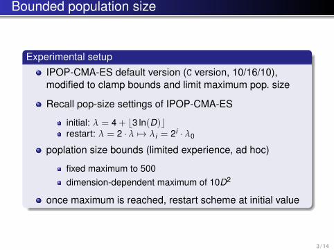
Experimental setupIPOP-CMA-ES default version (C version, 10/16/10),modified to clamp bounds and limit maximum pop. size

Recall pop-size settings of IPOP-CMA-ES

initial: λ = 4 + b3 ln(D)crestart: λ = 2 · λ 7→ λi = 2i · λ0

poplation size bounds (limited experience, ad hoc)

fixed maximum to 500dimension-dependent maximum of 10D2

once maximum is reached, restart scheme at initial value

3 / 14

Significant differences ERT

2 3 5 10 20 400

1

2

3

4

5

6

7

8

ftarget=1e-08

4 Skew Rastrigin-Bueche separ

2 3 5 10 20 400

1

2

3

4

5

6

7

ftarget=1e-08

19 Griewank-Rosenbrock F8F2

2 3 5 10 20 400

1

2

3

4

5

6

ftarget=1e-08

20 Schwefel x*sin(x)

2 3 5 10 20 400

1

2

3

4

5

6

7

ftarget=1e-08

24 Lunacek bi-Rastrigin

IP-10DDrIPIP-500

4 / 14

“Visible” differences

2 3 5 10 20 400

1

2

3

4

5

6

7

8

ftarget=1e-08

3 Rastrigin separable

2 3 5 10 20 400

1

2

3

4

5

6

ftarget=1e-08

16 Weierstrass

2 3 5 10 20 400

1

2

3

4

5

6

7

ftarget=1e-08

21 Gallagher 101 peaks

2 3 5 10 20 400

1

2

3

4

5

6

7

ftarget=1e-08

22 Gallagher 21 peaks

On many functions population-size bounds too loose to makean effect (apparently f1, f2, f4− f15, f17, f18)

5 / 14

“Visible” differences

2 3 5 10 20 400

1

2

3

4

5

6

7

8

ftarget=1e-08

3 Rastrigin separable

2 3 5 10 20 400

1

2

3

4

5

6

ftarget=1e-08

16 Weierstrass

2 3 5 10 20 400

1

2

3

4

5

6

7

ftarget=1e-08

21 Gallagher 101 peaks

2 3 5 10 20 400

1

2

3

4

5

6

7

ftarget=1e-08

22 Gallagher 21 peaks

On many functions population-size bounds too loose to makean effect (apparently f1, f2, f4− f15, f17, f18)

5 / 14

Tuning IPOP-CMA-ES

Tuning setup

use D = 10 functions from SOCO special issue

removed Sphere, Rosenbrock, Rastrigin, Schwefel 1.2from SOCO set error :-( Schaffer, f17

default version of irace

tuning budget: 5000 runs of IPOP-CMA-ES each of100D = 1000 function evaluations

short runs because same tuned version is used forexpensive scenario

measured cost function: evaluation function valueat end of trial

we are aware: wrong target for BBOB, not many parameterstuned, maybe wrong algorithm overall, etc.

. . . more to come . . .

6 / 14

Tuning IPOP-CMA-ES

Tuning setup

use D = 10 functions from SOCO special issue

removed Sphere, Rosenbrock, Rastrigin, Schwefel 1.2from SOCO set error :-( Schaffer, f17

default version of irace

tuning budget: 5000 runs of IPOP-CMA-ES each of100D = 1000 function evaluations

short runs because same tuned version is used forexpensive scenario

measured cost function: evaluation function valueat end of trial

we are aware: wrong target for BBOB, not many parameterstuned, maybe wrong algorithm overall, etc.

. . . more to come . . .6 / 14

Tuning IPOP-CMA-ES

Parameter Internal parameter default tuneda Init pop size: λ0 = 4 + ba ln(D)c 3 2.675b Parent size: µ = bλ/bc 2 1.351c Init step size: σ0 = c · (B − A) 0.5 0.102d IPOP factor: ipop = d 2 2.88e stopTolFun = 10e −12 −8.607f stopTolFunHist = 10f −20 −14.77g stopTolX = 10g −12 −9.529

Following comparison

default IPOP-CMA-ES

IPOP-CMA-ES with pop. size bound 10D2

IPOP-CMA-ES with pop. size bound 10D2, tuned

7 / 14

Tuning IPOP-CMA-ES

Parameter Internal parameter default tuneda Init pop size: λ0 = 4 + ba ln(D)c 3 2.675b Parent size: µ = bλ/bc 2 1.351c Init step size: σ0 = c · (B − A) 0.5 0.102d IPOP factor: ipop = d 2 2.88e stopTolFun = 10e −12 −8.607f stopTolFunHist = 10f −20 −14.77g stopTolX = 10g −12 −9.529

Following comparison

default IPOP-CMA-ES

IPOP-CMA-ES with pop. size bound 10D2

IPOP-CMA-ES with pop. size bound 10D2, tuned

7 / 14

Significant differences ERT

2 3 5 10 20 40

0

1

2

3

ftarget=1e-08

1 Sphere

texp

IP

IP-10DDr

2 3 5 10 20 400

1

2

3

4

ftarget=1e-08

2 Ellipsoid separable

2 3 5 10 20 400

1

2

3

4

5

6

ftarget=1e-08

7 Step-ellipsoid

2 3 5 10 20 400

1

2

3

4

ftarget=1e-08

9 Rosenbrock rotated

2 3 5 10 20 400

1

2

3

4

ftarget=1e-08

10 Ellipsoid

2 3 5 10 20 400

1

2

3

4

ftarget=1e-08

11 Discus

2 3 5 10 20 400

1

2

3

4

ftarget=1e-08

14 Sum of different powers

2 3 5 10 20 400

1

2

3

4

5

ftarget=1e-08

16 Weierstrass

2 3 5 10 20 400

1

2

3

4

ftarget=1e-08

17 Schaffer F7, condition 10

2 3 5 10 20 400

1

2

3

4

5

6

ftarget=1e-08

20 Schwefel x*sin(x)

2 3 5 10 20 400

1

2

3

4

5

6

7

ftarget=1e-08

22 Gallagher 21 peaks

2 3 5 10 20 400

1

2

3

4

5

6

7

8

ftarget=1e-08

24 Lunacek bi-Rastrigin

texp

IP

IP-10DDr

8 / 14

General scenario

0 1 2 3 4 5 6 7 8log10 of (# f-evals / dimension)

0.0

0.2

0.4

0.6

0.8

1.0Pro

port

ion o

f fu

nct

ion+

targ

et

pair

s

IP

IP-10DDr

best 2009

texpf1-24,3-D

0 1 2 3 4 5 6 7 8log10 of (# f-evals / dimension)

0.0

0.2

0.4

0.6

0.8

1.0

Pro

port

ion o

f fu

nct

ion+

targ

et

pair

s

IP

IP-10DDr

texp

best 2009f1-24,5-D

0 1 2 3 4 5 6 7 8log10 of (# f-evals / dimension)

0.0

0.2

0.4

0.6

0.8

1.0

Pro

port

ion o

f fu

nct

ion+

targ

et

pair

s

IP

IP-10DDr

texp

best 2009f1-24,10-D

0 1 2 3 4 5 6 7 8log10 of (# f-evals / dimension)

0.0

0.2

0.4

0.6

0.8

1.0

Pro

port

ion o

f fu

nct

ion+

targ

et

pair

s

IP

IP-10DDr

texp

best 2009f1-24,20-D

9 / 14

Expensive scenario

no changes, same algorithm (tuned IPOP-CMA-ES withmaximum population size bound (here not effective)

just a different look at the same data

Motivation: direct search may not be so bad after all . . .

10 / 14

Expensive scenario

no changes, same algorithm (tuned IPOP-CMA-ES withmaximum population size bound (here not effective)

just a different look at the same data

Motivation: direct search may not be so bad after all . . .

10 / 14

Expensive scenario

no changes, same algorithm (tuned IPOP-CMA-ES withmaximum population size bound (here not effective)

just a different look at the same data

Motivation: direct search may not be so bad after all . . .

10 / 14

Expensive scenario, comparison to defaultIPOP-CMA-ES

1e−01 1e+00 1e+01 1e+02 1e+03

1e−

01

1e+

00

1e+

01

1e+

02

1e+

03

texp (<1: 6 times)

def (<

1: 1

tim

es)

−Win 21 +

−Lose 3

−Draw 0

#FEs/D=0.5

0.2 0.4 0.6 0.8 1.0

0.5

0.7

0.9

1e−01 1e+00 1e+01 1e+02 1e+03

1e−

01

1e+

00

1e+

01

1e+

02

1e+

03

texp (<1: 5 times)def (<

1: 1

tim

es)

−Win 21 +

−Lose 1

−Draw 2

#FEs/D=1.2

0.2 0.4 0.6 0.8 1.0

0.5

0.7

0.9

1e−01 1e+00 1e+01 1e+02 1e+03

1e−

01

1e+

00

1e+

01

1e+

02

1e+

03

texp (<1: 4 times)

def (<

1: 2

tim

es)

−Win 19 +

−Lose 4

−Draw 1

#FEs/D=3.0

0.2 0.4 0.6 0.8 1.0

0.5

0.7

0.9

1e−01 1e+00 1e+01 1e+02 1e+03

1e−

01

1e+

00

1e+

01

1e+

02

1e+

03

texp (<1: 3 times)

def (<

1: 3

tim

es)

−Win 20 +

−Lose 4

−Draw 0

#FEs/D=10

0.2 0.4 0.6 0.8 1.0

0.5

0.7

0.9

1e−01 1e+00 1e+01 1e+02 1e+03

1e−

01

1e+

00

1e+

01

1e+

02

1e+

03

texp (<1: 2 times)

def (<

1: 2

tim

es)

−Win 12

−Lose 11

−Draw 1

#FEs/D=50

0.2 0.4 0.6 0.8 1.0

0.5

0.7

0.9

1e−01 1e+00 1e+01 1e+02 1e+03

1e−

01

1e+

00

1e+

01

1e+

02

1e+

03

texp (<1: 20 times)def (<

1: 9

tim

es)

−Win 93 +

−Lose 23

−Draw 4

Summary

0.2 0.4 0.6 0.8 1.0

0.5

0.7

0.9

11 / 14

Expensive scenario, comparison to ImmCMA-ES

1e−01 1e+00 1e+01 1e+02 1e+03

1e−

01

1e+

00

1e+

01

1e+

02

1e+

03

texp (<1: 6 times)

imm

cm

a (

<1: 6

tim

es) −Win 13

−Lose 10

−Draw 1

#FEs/D=0.5

0.2 0.4 0.6 0.8 1.0

0.5

0.7

0.9

1e−01 1e+00 1e+01 1e+02 1e+03

1e−

01

1e+

00

1e+

01

1e+

02

1e+

03

texp (<1: 5 times)

imm

cm

a (

<1: 2

tim

es) −Win 16 +

−Lose 8

−Draw 0

#FEs/D=1.2

0.2 0.4 0.6 0.8 1.0

0.5

0.7

0.9

1e−01 1e+00 1e+01 1e+02 1e+03

1e−

01

1e+

00

1e+

01

1e+

02

1e+

03

texp (<1: 4 times)

imm

cm

a (

<1: 3

tim

es) −Win 13

−Lose 10

−Draw 1

#FEs/D=3.0

0.2 0.4 0.6 0.8 1.0

0.5

0.7

0.9

1e−01 1e+00 1e+01 1e+02 1e+03

1e−

01

1e+

00

1e+

01

1e+

02

1e+

03

texp (<1: 3 times)

imm

cm

a (

<1: 3

tim

es) −Win 8

−Lose 15

−Draw 1

#FEs/D=10

0.2 0.4 0.6 0.8 1.0

0.5

0.7

0.9

1e−01 1e+00 1e+01 1e+02 1e+03

1e−

01

1e+

00

1e+

01

1e+

02

1e+

03

texp (<1: 2 times)

imm

cm

a (

<1: 3

tim

es) −Win 5 +

−Lose 18

−Draw 1

#FEs/D=50

0.2 0.4 0.6 0.8 1.0

0.5

0.7

0.9

1e−01 1e+00 1e+01 1e+02 1e+03

1e−

01

1e+

00

1e+

01

1e+

02

1e+

03

texp (<1: 20 times)

imm

cm

a (

<1: 1

7 tim

es)

−Win 55

−Lose 61

−Draw 4

Summary

0.2 0.4 0.6 0.8 1.0

0.5

0.7

0.9

12 / 14

Expensive scenario, comparison to SMAC-BBOB

1e−01 1e+00 1e+01 1e+02 1e+03

1e−

01

1e+

00

1e+

01

1e+

02

1e+

03

texp (<1: 6 times)

sm

ac (

<1: 1

1 tim

es) −Win 9

−Lose 15

−Draw 0

#FEs/D=0.5

0.2 0.4 0.6 0.8 1.0

0.5

0.7

0.9

1e−01 1e+00 1e+01 1e+02 1e+03

1e−

01

1e+

00

1e+

01

1e+

02

1e+

03

texp (<1: 5 times)

sm

ac (

<1: 8

tim

es) −Win 14

−Lose 10

−Draw 0

#FEs/D=1.2

0.2 0.4 0.6 0.8 1.0

0.5

0.7

0.9

1e−01 1e+00 1e+01 1e+02 1e+03

1e−

01

1e+

00

1e+

01

1e+

02

1e+

03

texp (<1: 4 times)

sm

ac (

<1: 5

tim

es) −Win 14 +

−Lose 8

−Draw 2

#FEs/D=3.0

0.2 0.4 0.6 0.8 1.0

0.5

0.7

0.9

1e−01 1e+00 1e+01 1e+02 1e+03

1e−

01

1e+

00

1e+

01

1e+

02

1e+

03

texp (<1: 3 times)

sm

ac (

<1: 3

tim

es) −Win 17 +

−Lose 6

−Draw 1

#FEs/D=10

0.2 0.4 0.6 0.8 1.0

0.5

0.7

0.9

1e−01 1e+00 1e+01 1e+02 1e+03

1e−

01

1e+

00

1e+

01

1e+

02

1e+

03

texp (<1: 2 times)

sm

ac (

<1: 3

tim

es) −Win 19 +

−Lose 5

−Draw 0

#FEs/D=50

0.2 0.4 0.6 0.8 1.0

0.5

0.7

0.9

1e−01 1e+00 1e+01 1e+02 1e+03

1e−

01

1e+

00

1e+

01

1e+

02

1e+

03

texp (<1: 20 times)

sm

ac (

<1: 3

0 tim

es) −Win 73 +

−Lose 44

−Draw 3

Summary

0.2 0.4 0.6 0.8 1.0

0.5

0.7

0.9

13 / 14

Conclusions

limiting max. population size of IPOP-CMA-ES can help

tuning can further improve performance

main differences on weakly structured multi-modalfunctions (also other benchmarks such as CEC’05 / ’13)

IPOP-CMA-ES anyway rather robust

14 / 14