Bounded Gaps Between Consecutive Primes

John Musson

Trinity College

MMath

Hilary 2015

Abstract

In 2013 Yitang Zhang proved a weak version of the Twin Prime Conjecture,stating that there are infinitely many pairs of consecutive prime numberswithin a bounded distance from each other. Zhang’s bound was 70,000,000,but within a year James Maynard had produced a proof using significantlydifferent methods that reduced this bound to 600. This dissertation will givean exposition of Maynard’s recent paper, in a way that will make it accessibleto undergraduate or recently graduated number theorists.

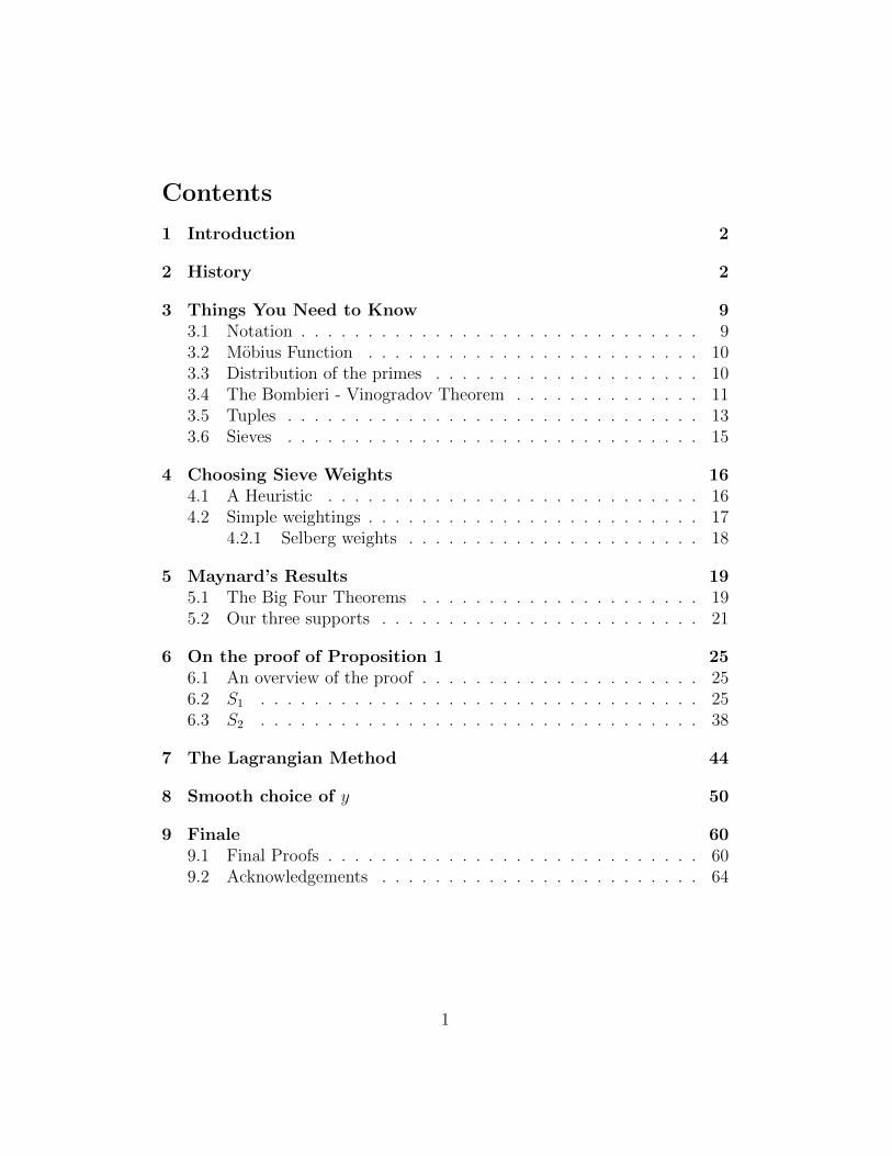
Contents

1 Introduction 2

2 History 2

3 Things You Need to Know 93.1 Notation . . . . . . . . . . . . . . . . . . . . . . . . . . . . . . 93.2 Mobius Function . . . . . . . . . . . . . . . . . . . . . . . . . 103.3 Distribution of the primes . . . . . . . . . . . . . . . . . . . . 103.4 The Bombieri - Vinogradov Theorem . . . . . . . . . . . . . . 113.5 Tuples . . . . . . . . . . . . . . . . . . . . . . . . . . . . . . . 133.6 Sieves . . . . . . . . . . . . . . . . . . . . . . . . . . . . . . . 15

4 Choosing Sieve Weights 164.1 A Heuristic . . . . . . . . . . . . . . . . . . . . . . . . . . . . 164.2 Simple weightings . . . . . . . . . . . . . . . . . . . . . . . . . 17

4.2.1 Selberg weights . . . . . . . . . . . . . . . . . . . . . . 18

5 Maynard’s Results 195.1 The Big Four Theorems . . . . . . . . . . . . . . . . . . . . . 195.2 Our three supports . . . . . . . . . . . . . . . . . . . . . . . . 21

6 On the proof of Proposition 1 256.1 An overview of the proof . . . . . . . . . . . . . . . . . . . . . 256.2 S1 . . . . . . . . . . . . . . . . . . . . . . . . . . . . . . . . . 256.3 S2 . . . . . . . . . . . . . . . . . . . . . . . . . . . . . . . . . 38

7 The Lagrangian Method 44

8 Smooth choice of y 50

9 Finale 609.1 Final Proofs . . . . . . . . . . . . . . . . . . . . . . . . . . . . 609.2 Acknowledgements . . . . . . . . . . . . . . . . . . . . . . . . 64

1

1 Introduction

The prime numbers have fascinated mathematicians since antiquity: fromEuclid’s proof of their boundlessness to the Riemann Hypothesis, they couldconsistently claim the title of the greatest enigma in mathematics. Like manyof the best mathematical problems, the Twin Prime Conjecture is simple tostate yet devilishly tricky to prove - in fact, it is still eluding proof.

Conjecture (Twin Prime Conjecture). There are infinitely many primesp, such that p+ 2 is also a prime.

Hundreds of thousands of twin primes have been found usingcomputational methods; examples include the well known pairs (3, 5) and(11, 13) and the lesser known pair (101999, 102001).

It is unclear when the notion of twin primes was first coined. Someattribute it to Euclid (which would make this one of mathematics’oldest unsolved problems), however the earliest observance in mathematicalliterature, according to a history of the problem by Nazardonyavi [13], canbe found in Polignac’s “Six propositions arithmologiques deduites du cribled’Eratosthene” [14], in which he proposes the more general conjecture:

Conjecture (Polignac, 1849). For any positive even number n, there areinfinitely many consecutive primes p and q such that q − p = n.

With n = 2 this is exactly the Twin Prime Conjecture. Developmentssince 2013 have finally put us within touching distance of these conjectures:for the first time we have an unconditional, finite bound on the minimumdifference between arbitrarily large consecutive primes. This dissertation willmostly be a detailed exposition of a number of recent theorems by Maynard[11]; however we’ll begin with a short history of work in this area beforecovering the mathematical techniques used in the proof and then continuingon to the theorems themselves.

2 History

1793 - Gauss

Considered by many to be the greatest mathematician of all time, CarlFriedrich Gauss made huge contributions to many areas of mathematics in his

2

lifetime. His Disquisitiones Arithmeticae, which he published aged only 24,changed number theory from a collection of results into a recognised branchof mathematics. Gauss solved the ancient problem of how to construct a17-gon with just ruler and compass; introduced modular arithmetic and,after calculating a list of primes up to 3,000,000, conjectured what wouldbecome known as the prime number theorem. The following theorem wasindependently proposed by Legendre around the same time albeit with themore slowly converging estimate of x

log x:

Theorem (Prime Number Theorem). Let π(x) be the number of primesbelow x, and let

Li(x) : =

ˆ x

2

1

log(t)dt.

Then

limx→∞

π(x)

Li(x)= 1.

Number theory really blossomed following Gauss. Throughout the 19th

century mathematicians such as Galois and Dirichlet developed whole newsubfields, making greater levels of rigour and abstraction commonplace. Thecrowning achievement of 19th century number theory however, was probablythe introduction of complex analytical methods with the work of Riemannconcerning his now infamous zeta function in 1859. The Generalised RiemannHypothesis (GRH), stating that every zero of certain functions, like theRiemann zeta function, lies on the line Re(x) = 1

2, has stood the test of

time and remains one of the great open problems of modern mathematics.It was a result of work done by Riemann, followed by Hadamard and de laVallee Poussin in 1896, that finally supplied a proof to Gauss’ then centuryold conjecture which created the Prime Number Theorem above.

1965 - Bombieri - Vinogradov

Jumping ahead to the middle of the next century, number theory hadprogressed significantly. While the GRH was (and still is) unreachable inits full capacity, many related results had come to light, one which is theBombieri - Vinogradov Theorem. Although Bombieri and A. Vinogradov(there were two Vinogradovs in 20th century Russian mathematics, so it paysto be specific) never published a joint paper, each published slightly differentresults in the same year, a refinement of which is the Bombieri - Vinogradov

3

Theorem [21]. In general terms, the Bombieri - Vinogradov Theorem givesan upper bound for the average number of primes less than a given x ∈ Nin a particular residue class modulo q ≤ Q for some Q ≤ x. Specifically,defining

θ(x; q, a) :=∑p≤x

p primep≡a mod q

log(p),

a weighted sum for the number of primes less than x in the residue class amodulo q, we have:

Theorem (Bombieri - Vinogradov, 1965). The following inequality holds

for Q ≤ x12 (log x)−C for some positive constant C with A a positive constant

depending on C: ∑q≤Q

max(a,q)=1

∣∣∣∣θ(x; q, a)− x

φ(q)

∣∣∣∣� x

(log(x))A.

We will give a more detailed explanation of the precise meaning andconsequences of this theorem in Section 3.4.

The exponent of x for which this theorem holds is called the level ofdistribution of the primes. It is often referred to as θ, not to be confusedwith the function θ(x; q, a).

There has been a lot of work attempting to extend θ past 12, in particular

to prove a conjecture of Elliott - Halberstam [2]:

Conjecture (Elliott - Halberstam Conjecture, 1970). The Bombieri -Vinogradov Theorem holds for all Q < x(log x)−C.

However no proof is yet known.One of the major ingredients of recent work extending the Bombieri -

Vinogradov Theorem was improving the bound to x12+ω for an arbitrarily

small ω > 0, albeit with a modified version of the Bombieri - Vinogradovstatement, which was in turn sufficient to give bounded gaps between primenumbers. On the other hand Friedlander and Granville [3] showed thatthe bound of x is maximal (in particular, the statement does not hold forQ ≤ x(log x)−C for any fixed C). The minimum distance of bounded gaps isconsiderably reduced if one assumes the full Elliott - Halberstam conjecture,though the existence of such a minimum depends only on Bombieri -Vinogradov.

4

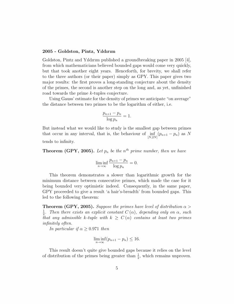
2005 - Goldston, Pintz, Yıldırım

Goldston, Pintz and Yıldırım published a groundbreaking paper in 2005 [4],from which mathematicians believed bounded gaps would come very quickly,but that took another eight years. Henceforth, for brevity, we shall referto the three authors (or their paper) simply as GPY. This paper gives twomajor results: the first proves a long-standing conjecture about the densityof the primes, the second is another step on the long and, as yet, unfinishedroad towards the prime k-tuples conjecture.

Using Gauss’ estimate for the density of primes we anticipate “on average”the distance between two primes to be the logarithm of either, i.e.

pn+1 − pnlog pn

= 1.

But instead what we would like to study is the smallest gap between primesthat occur in any interval, that is, the behaviour of inf

[N,2N ](pn+1 − pn) as N

tends to infinity.

Theorem (GPY, 2005). Let pn be the nth prime number, then we have

lim infn→∞

pn+1 − pnlog pn

= 0.

This theorem demonstrates a slower than logarithmic growth for theminimum distance between consecutive primes, which made the case for itbeing bounded very optimistic indeed. Consequently, in the same paper,GPY proceeded to give a result ‘a hair’s-breadth’ from bounded gaps. Thisled to the following theorem:

Theorem (GPY, 2005). Suppose the primes have level of distribution α >12. Then there exists an explicit constant C (α), depending only on α, such

that any admissible k-tuple with k ≥ C (α) contains at least two primesinfinitely often.

In particular if α ≥ 0.971 then

lim infn→∞

(pn+1 − pn) ≤ 16.

This result doesn’t quite give bounded gaps because it relies on the levelof distribution of the primes being greater than 1

2, which remains unproven.

5

The tools used by GPY were almost a decade old when their paper waspublished. Their input was to apply Heath-Brown’s generalization of theSelberg sieve (which we will define in the next section), for estimating thenumber of prime factors in any admissible tuple [8] (another definition thatwill be addressed in Section 3), to the task of estimating the existence ofmultiple primes in the tuple. The publication of this work prompted a greatdeal of mathematical activity attempting to remove the conditionality on anunproven statement. However, little progress was made for the next eightyears.

2013 - Zhang

Yitang Zhang rocketed from obscurity as a lecturer at the University of NewHampshire to international fame (for a mathematician) at the remarkableage of 57 upon the publication of his paper providing the first proof of finitegaps between prime numbers [23].

Theorem (Zhang, 2013). Let pn be the nth prime number, it is proved that

lim infn→∞

(pn+1 − pn) ≤ 70, 000, 000.

This may seem a far cry from the twin primes conjecture, but 70, 000, 000is considerably closer to 2 than infinity and his paper explicitly left significantroom for others to sharpen his bounds.

The original part of Zhang’s proof was not to show that the primeshave level of distribution α > 1

2(which would have made the GPY method

sufficient), but instead to use a stronger version of Bombieri - Vinogradovpublished by Bombieri - Friedlander - Iwaniec in the late 1980’s. Applicableonly with an additional restriction on the prime factors of certain summands,many had thought it could be easily merged with GPY but each requiredconditions incompatible with the other. Following GPY, Iwaniec himself hadtried, but failed, to remove the conditions on his paper. The most impressivething about Zhang’s paper, was arguably how he managed to take the workof leading mathematicians in the field, and prove something with a methodthey had abandoned [22]. A great exposition of Zhang’s proof was writtenby Granville and can be found at [7].

6

2014 - Polymath

As soon as Zhang’s work was available to the wider mathematical communityit was devoured by some of the most prominent mathematicians in the area,and within two weeks the bound had been brought below 60,000,000 byMark Lewko and then Thomas Trudgian [20]. The remarkable speed ofprogress and the potential for lowering such an important bound inspiredmathematicians to work together to form a Polymath project.

The Polymath Project was conceived in 2009 by Tim Gowers [6]and Michael Nielsen as an experiment in massively collaborative onlinemathematics. The premise was that most mathematical collaborations aredone between two, three or in rare cases four co-authors (with the notableexception of the Bourbaki group in the mid 1930s), but there are obviousadvantages to having input from a larger pool of mathematicians; includinggenerating a greater knowledge base, allowing people to focus on singleparts of a work, and encouraging different approaches to the same problem.Polymath is still a work in progress and its projects have had varying levels ofsuccess. Of the nine full projects since its inception, six have produced partialanswers or answers to related problems and three have created publishableresults, including Polymath8, the follow up to Zhang’s work.

The Polymath8 project was headed up by Fields medalist Terence Taoon his blog [19]1 and the brief he gave was twofold: firstly to understand andclarify Zhang’s argument and secondly to improve the numerical bound ongaps between primes. The project was hugely successful, with the first writeup totalling 163 pages and giving a reduction of Zhang’s bound to 4,680. Butover the three months it was being written up (again, by a group of people,in the spirit of Polymath), a new paper came to light: written by JamesMaynard, the proofs involved quite different methods to Zhang and broughtthe upper bound down to 600 using the Bombieri - Vinogradov Theorem (notZhang’s stronger alternative) and an improvement on GPY. While the writeup of Polymath8 [15] was completed, Polymath8b was instantly spawnedto see how their previous work could be applied to Maynard’s theorems togive an even stronger result. At the conclusion of Polymath8b, the bestunconditional bound for the smallest gap between consecutive prime numbersis 246 [16].

1Due to the nature of the blog style it is impossible to supply a single reference page,this reference gives all the pages related to Polymath8, however the reader is encouragedto browse T.Tao’s wordpress articles

7

Theorem (Polymath, 2014). Let pn be the nth prime number,unconditionally we have

lim infn→∞

(pn+1 − pn) ≤ 246.

They also gave a number of explicit bounds for lim inf(pn+k − pn) for1 ≤ k ≤ 5 and a bound for general k ∈ N however we shall leave the moregeneral cases in favour of the main focus of this paper.

2014 - Maynard

After finishing his DPhil at Oxford under Roger Heath-Brown, JamesMaynard took up a postdoctoral fellowship at the University of Montreal.While there, he finished a considerably more simple proof than Zhang’s ofa finite bound for lim inf(pn+1 − pn), which also provided the significantlylower number of 600 mentioned above. Slightly weaker results wereachieved independently by Terence Tao using similar methods at the sametime causing some to refer to the “Maynard-Tao method”. This paperwill go through Maynard’s proof and explain it at a level accessible toundergraduates or recent graduates in the area.

A Road Map for this Paper

In Section 3 we shall establish some notation as well as cover a few keymathematical tools for dealing with prime number theory. In Section 4we shall look at some simple sieve weights and how we must adjust toget a sufficient level of complexity to produce interesting results. Section5 will state the four theorems proven in Maynard’s paper, along with thepropositions necessary for proving them. Sections 6,7 and 8 together willgive us a proof of the main proposition. Finally Section 9 will pull the threepropositions together to prove the four theorems as well as discuss furtherprogress.

8

3 Things You Need to Know

The first thing we are going to do is establish the notation we are going touse throughout the paper and take some time explaining a few of them.

3.1 Notation

All variables a, ai, b, bi, d, di, e, ei, r, ri, j, k, n,N,W and x should be assumedto lie in the natural numbers unless explicitly specified otherwise.p: a prime numberpn: the nth prime numberε, δ any sufficiently small, positive numberyr: yr1,...,rk , a number depending on r1, . . . , rk and we will use these twonotations interchangeablya | b: a divides ba - b: a does not divide ba ≡ b (p): a is congruent to b modulo pµ(x): The Mobius function (covered in Section 3.2)

ϕ(x) :∏p|x

p prime

(p− 1)

g(x) :∏p|x

p prime

(p− 2)

φ(x): the Euler Totient function φ(q) = |{p < q : (p, q) = 1}|θ(x): the first Chebyshev function, defined in Section 3.3θ(x; q, a): defined in Section 3.3τj(a): the divisor function (the number of ways of writing a as a product ofj factors)∑d1,...,dk

: the sum over all possible sets {d1, . . . , dk}

H = (h1, . . . , hk): a k-tuple (covered in Section 3.4), assumed to be fixed(a, b): the highest common factor of a and b (at no point are (a, b) and(h1, . . . , hk) used together so no confusion should arise)[a, b]: the lowest common multiple of a and bdxe: the roof of x, the smallest integer greater than xOA: big O asymptotic notation, depending on A. If no A is specified then itmay depend on k and H

9

3.2 Mobius Function

The Mobius function is defined as follows:

µ(x) :=

1 x = 1

1 x is square-free and has an even number of prime factors

−1 x is square-free and has an odd number of prime factors

0 x is not square-free.

It can be used as an indicator of whether a positive integer n is 1 or not:

∑d|n

µ(d) =

{1 n = 1

0 n > 1

It is multiplicative for coprime numbers, that is, µ(a)µ(b) = µ(ab).Clearly if a and b are not coprime then their product is not squarefree andin that case µ(ab) = 0.

3.3 Distribution of the primes

Understanding fully the distribution of the primes is beyond currentmathematics; however we have had estimates for how they propagate ingeneral since the 18th century.

Let π(x) be the prime counting function that increments by 1 for everyprime between 0 and x. In 1798 Legendre [10] estimated that

x

log(x)− 1.08366∼ π(x).

Almost 50 years later, Dirichlet (in communication with Gauss) used hisintegral

Li(x) :=

ˆ x

2

1

log(t)dt

for the same approximation. The difference between Li(x) and π(x) ismuch smaller than Legendre’s function; however convergence in both casesis equivalent when it comes to the quotient. This means the Prime NumberTheorem can be stated as either:

limx→∞

π(x)x

log(x)

= 1,

10

or

limx→∞

π(x)

Li(x)= 1.

We define the Chebyshev function, a weighted prime counting function,

θ(x) :=∑p≤x

p prime

log(p)

and, as mentioned previously,

θ(x; q, a) :=∑p≤x

p primep≡a (q)

log(p).

It turns out that the Prime Number Theorem is equivalent to the statementθ(x)x

∼ 1 as x → ∞ (a proof of this can be found in [9] page 83, albeit inGerman).

3.4 The Bombieri - Vinogradov Theorem

We now provide the motivation behind the Bombieri - Vinogradov Theoremwhich we stated in the previous section. We know that being able to estimateπ(x) is equivalent to being able to estimate θ(x), but unfortunately both arerather hard to do. Instead we have the Bombieri - Vinogradov Theoremwhich we now have all the tools necessary to understand. The precise natureof the function used in the Bombieri - Vinogradov Theorem takes a littleexplaining:

1. First, consider how we anticipate the primes below x to be distributedmodulo q for any given q. If the primes were a totally randomdistribution we could conjecture that |{p ≤ x : p = a mod q}| = π(x)

φ(q)

where φ(q) is the Euler totient function (φ(q) = |{p < q : (p, q) = 1}|);

2. From the Prime Number Theorem we have π(x) → xlog(x)

;

3. Finally, the weighting of each prime from 1 to log(p) in the definition

of θ gives us θ(x; q, a) = π(x)φ(q)

log(x) ≈ xφ(x)

.

11

We do in fact have results saying exactly this, but the nature of the relation≈ naturally leaves us with errors to minimise. Let’s have a look at how smallwe can make these errors:

The prime number theorem can be extended to a version for arithmeticprogressions in the same way that θ(x) is extended to θ(x; q, a). From thiswe get the following (see [12, Corollary 11.21] for a proof):

Corollary 3.1. Let x, q, a ∈ N and A > 0 be such that x and q are coprimeand q ≤ logA x, then

θ(x; q, a) =x

φ(q)+OA(x(log x)

−A).

If, however, we allow ourselves to assume the full Generalised RiemannHypothesis, we get a much stronger bound [12, Corollary 13.8].

Corollary 3.2. Assume the Generalised Riemann Hypothesis and letx, q, a,∈ N and A > 0 be such that x and q are coprime and q ≤ logA x,then

θ(x; q, a) =x

φ(q)+OA

(x

12 (log x)2

).

Unfortunately we can’t just assume the GRH is true, but luckily for us,Bombieri - Vinogradov is a completely unconditional, yet very strong, result.What this gives us is that ‘on average’ Corollary 3.2 is true (without firstassuming GRH); in this case, by ‘on average’ we mean that if we take the sum

over all q ≤ xm, we expect the error to be no larger than OA

(xmx

12 (log x)2

).

We must note, however, that Bombieri - Vinogradov extends only to m < 12.

For each q, Bombieri - Vinogradov takes the worst case, the residue classa with either the most or the fewest primes (depending on which is furtherfrom x

φ(q)) and we sum over all q ≤ Q; this allows us a little leeway, for some

q it may be the case that

max(a,q)=1

|θ(x; q, a)− x

φ(q)| > x

(log(x)AQ>

x12

log(x)A.

That is, the difference on the LHS is greater than the magnitude of errorgiven in Corollary 3.2, but the theorem tells us that this is not the case ingeneral.

The statement is as follows [21]:

12

Theorem (Bombieri - Vinogradov, 1965). For all x in N, and all

positive constants A and C = f(A), the following holds if Q < x12 (log x)−C:∑

q≤Q

max(a,q)=1

|θ(x; q, a)− x

φ(q)| � x

(log(x))A.

Finally, for completeness, we restate that if Bombieri - Vinogradovholds for Q < xθ(log x)−C for some constant C ∈ R, then θ is the levelof distribution of the primes, and we give the extension of this result(conjectured a few years later) that has been left to future mathematiciansto prove [2]:

Conjecture (Elliott - Halberstam Conjecture, 1970). The Bombieri -Vinogradov Theorem holds for all Q < x(log x)−C .

We include this again because, once proved, it will overtake the Bombieri- Vinogradov as the prominent result in the area. For this reason, mostpapers on bounding prime numbers, and certainly all those referenced in thisdissertation, give two results, one assuming Elliott - Halberstam and oneattainable with only current methods.

3.5 Tuples

The Bombieri - Vinogradov Theorem concerns arithmetic progressions so wenow develop some terminology to represent different progressions.

Consider an ordered set of distinct, non-negative integers, for exampleH = (0, 1, 5). Then the corresponding tuples are all sets {n, n + 1, n + 5},(n ∈ N), so our H stands for all the sets of integers with the same additivepattern. A k-tuple helpfully contains k elements and we have a prime k-tuplewhen every element is prime. The length of a tuple is the difference betweenthe first and last element.

A more relevant example would be the twin primes, which are representedby the tuple (0, 2): the Twin Prime Conjecture is exactly the statement thatthis tuple corresponds to infinitely many prime 2-tuples.

Conjecture (Prime k-tuples Conjecture). For any admissible primek-tuple, (h1, h2, . . . , hk) , the numbers {n+ hi}ki=1 are all prime for infinitelymany n in N.

13

A tuple H = (h1, h2, . . . , hk) is ‘admissible’ if, for every prime p, there issome integer ap less than p such that no hn in H is congruent to ap modulop. That is, if you reduced every element of H to its residue mod p, at leastone number from 0 to p− 1 is not in H; equivalently, any set correspondingto H may be referred to as an ‘admissible’ set. For every prime p greaterthan k, this must be the case as there are more residue classes than elementsin H. So for any finite H, whether it is admissible or not is a finite check. Aset is inadmissible if it is not admissible.

Being admissible is important because only admissible tuples have achance of representing infinitely many prime k-tuples. Looking back to ouroriginal H we see it contains an element from every residue class modulo3. Considering the general set {n, n + 1, n + 5} we note if n is prime it iseither 2, or odd, in which case n+ 5 is even (and not 2) so not prime, hencethe only prime tuple represented by H is {2, 3, 7} and H becomes somewhatredundant in the search for infinite sets of primes with specific differences.This motivates our first proposition:

Proposition 3.1. For an inadmissible tuple there are at most kcorresponding prime k-tuples.

Proof. Let H = (h1, h2, . . . , hk) be an inadmissible tuple, ordered so thathn−1 < hn for every n ≤ k. Without loss of generality we may let h1 be thesmallest number such that all the hi are prime, recall we are only interestedin the differences hi − h1 in our definition of H )if no such h1 exists thenthere are no corresponding prime k-tuples and we are done).By definition of inadmissible, for some prime p < k, H contains every residueclass of p. Specifically, H always contains an element which is congruent to0 mod p. That is, H contains an element which is a multiple of p. Either itis p, or it is not prime.

As {h1, h2, . . . , hk} contains only primes, then from above it contains p,say ht. As elements in H are in increasing order, if, for some integer n,n + hs ≡ 0 (p) for any s > t then n + hs must be greater than p and thusbe a multiple of p and clearly not be prime. Hence, there are at most t − 1integers greater than 0 that may produce a set containing only primes, namely(p− ht−1), (p− ht−2), . . . , (p− h1). As t is arbitrary but bounded above byk, we get the lemma.

The idea of ‘twin primes’ or even consecutive primes does notfundamentally rely on tuples, because we’re only looking for two primes, not

14

k of them all together. Working with tuples gives us an instant generalisationof our theorems about consecutive primes to theorems about, for example,pn − pn+k.

3.6 Sieves

When a mathematician begins to learn about sieve theory they are usuallygiven the very unfortunate starting example of the sieve of Eratosthenes anda metaphor about pasta. It is unfortunate in two ways, firstly because itdoesn’t do what modern sieves do and secondly because it gives unrealisticexpectations about the power of the tool.

The sieve of Eratosthenes is a simple method for finding primes below anatural number n:

1. Write down the first n natural numbers,

2. Cross off the number 1,

3. Write the first uncrossed number on a separate list,

4. Cross off every multiple of that number,

5. Repeat steps 3 and 4 until every number is crossed off.

The first time you do step 3 you put the number 2 on your list, then cross offall the multiples of 2, next you will write down 3 and remove all of its productsand so on. The metaphor will tell the student who has just successfully foundall the primes up to n that they have taken their initial list, a pan full ofpasta (primes) that they want, and the water (composite numbers) that it’scooked in and poured it through a sieve leaving them with only a tasty meal;this is a rather unrealistic view of what modern sieve theory can achieve.

The sieve of Eratosthenes is very good at its job; the problem is thatto apply it to an arbitrarily large set of numbers takes an equally largeamount of time and, as our n tends to infinity, Eratosthenes’ sieve falls bythe wayside somewhat. Our focus will be on the Selberg sieve (also known asthe (Selberg) upper bound sieve, or the (Selberg) Λ2- sieve), a tool created in1947 by Atle Selberg. It differs from the sieve of Eratosthenes in that, insteadof telling you exactly which numbers are prime, given a set [N, 2N ] it givesa good estimate for how many are prime. Continuing our pasta metaphor,the Selberg sieve doesn’t remove all the water from our saucepan but instead

15

gives you a good estimate for how much is left. We will give a more detaileddescription of how the sieve works in the next section. Selberg used his sieveto give an upper bound for the number of primes remaining, but at the timeit didn’t produce the level of results he had been looking for and was laterreplaced in most mathematicians’ minds by more sophisticated methods. Somuch so, in fact, that in 1991 [18] Selberg described it as “now of historicinterest only”. However he was shortly proven wrong - just before the turnof the millennium, Roger Heath-Brown used a generalisation of the Selbergsieve in the search for prime tuples and this was later built on by GPY toset the scene for Zhang’s work.

4 Choosing Sieve Weights

4.1 A Heuristic

Assume we have an admissible set H = (h1, h2, . . . , hk). Then we want tofind n such that ‘many’ of the {n+ hi}ki=1 are prime.

We want to see how the number of primes in {n+ hi}ki=1changes as n →∞, so define

S :=∑n<N

∣∣∣{p : p ∈ {n+ hi}ki=1

}∣∣∣wn

for some, as yet undefined, weights wn ≥ 0.We begin with a look at possible sieve weights and discuss limitations of

the most obvious choices to motivate the weights we will eventually choose.A useful tool for this is the prime indicator function

1p(n) :=

{1, n prime

0, otherwise

and we consider the sum

Pn :=k∑

i=1

1p(n+ hi)

which counts the number of primes for each n. It may seem odd that we gofrom considering Pn, which is precisely the value we want to understand, toS, a seemingly more complicated expression. This is because Pn is “easy” to

16

understand only in a tautological sense: if we understood it or could evaluateit well, then we would know the truth of the prime k-tuples conjecture or, atthe very least, bounded gaps. Instead we work with the sum S which couldbe considered a weighted average over all the Pn in a given range.

We can then redefine S from the plan to be:

S :=∑

N≤n≤2N

(Pn −m)wn. (4.1)

The keen-eyed reader may notice that n in our sum no longer runs from 0up to N , but instead from N to 2N . We make this change because if we wentfrom 0, we would have to keep changing our sieve weights to deal with all thesmaller primes, so this simplifies things by giving our n a lower bound. Wewill in fact use an S different again from either of these in the forthcomingproofs, summing instead over n - W (where W =

∏p<D0

p is the productover all primes less than a certain constant), but these have the same effectand, to show the different options, we will continue to use (4.1) for now.

We want these weights to be large when Pn > m and small otherwise.If S > 0 as x → ∞ then at least one of the Pn must be making a positivecontribution, so there must be at least m primes in the bounded interval[n+ h1, n+ hk] for infinitely many n, m = 2 would be sufficient to give usbounded gaps, however it is good to work in slightly more generality. Thisleads us on to phase 2:

4.2 Simple weightings

Currently the only restriction we have on our weights is that they must benon-negative, but clearly this leaves rather a large range of options for ourwn; some of these will be better than others. Let’s begin with two trivialoptions: the simplest, and the most efficient.

1) The simplest case is when we add no weighting, or equivalently, auniform weighting. That is, we take wn = 1

Nfor all n. Then

S =∑

N≤n≤2N

(Pn −m)wn

=1

N

∑N≤n≤2N

(Pn −m)

17

by the prime number theorem, Pn → klog(N)

as N → ∞, giving,

=1

N

(Nk

log(N)−Nm

)=

k

log(N)−m

But,

limx→∞

(k

log(N)−m

)≤ 0

so (thankfully, else this dissertation would be cut rather short) we cannotget the relation we want (S > 0) without weights.

2) The other obvious and most optimistic case is to take

wn =

{1 Pn > m

0 otherwise.

If we could evaluate S with this weighting then we would immediatelyhave bounded gaps. However, as before when we had to move away fromevaluating Pn on its own, claiming we knew enough about wn to work with Swould also be equivalent to knowing the proof of the statement in advance.

4.2.1 Selberg weights

Having looked at the two most extreme cases, we look now for one that sitsin the middle. The Selberg sieve weights offer something we can evaluateand will eventually come to modify to get the results we want.

Selberg’s initial work was focused on looking at just 2-tuples and, on theface of it, this seems like the best way to find bounded gaps, seeing as a limiton finite gaps only requires two primes to be found. However, work since (inparticular, the work we shall cover here) has looked at k-tuples because theyoffer us a lot more flexibility on where the two primes may lie.

With this in mind we’ll jump immediately to the previously mentionedk-dimensional generalisation of the Selberg sieve developed by Heath-Brownin 1997 [8]. Heath-Brown wanted to study a function very similar to our Sabove and so tried to find a weighting where the negative part is small and

18

the positive part is calculable. This led him to use the upper bound sieve toevaluate the negative part, with the following weighting:

wn :=

∑d|∏

n+hid<R

λd

2

where

λd ≈

{µ(d) logk

(ξd

), for all d ≤ ξ

0, for all d > ξ,

with ξ here being x13−ε for a small positive ε. This was sufficient for the

results Heath-Brown was looking for but not enough to give bounded gaps.He notes in his paper that part of his analysis would break down if he tookthe exponent of x to be 1

2− ε and, as a result, his argument is somewhat

inefficient. On the other hand, he also says that Selberg suggests replacing∑d|∏k

i=1(n+hi)

λd

with ∑di|n+hi

λd1,...,dk

and this is exactly what Maynard did to gain the flexibility to establish muchstronger results.

5 Maynard’s Results

James Maynard produced four theorems, covering both the general case ofprime k-tuples and the specific case of consecutive primes, both with andwithout Elliott - Halberstam. The theorems fall into place relatively easilyafter we establish the corresponding propositions which will take up themajority of the remainder of this paper.

5.1 The Big Four Theorems

Theorem 1 is the specific and unconditional case that we are most interestedin: the case of consecutive primes given only θ < 1

2(recall: θ is the “level of

19

distribution of the primes” defined in Section 3.4). In Maynard’s paper it isgiven as 600, though he mentions this is not optimal, and since then therehave been refinements by Tao, Kowalski and others in the Polymath projectto bring this number down to 246 [16].

Theorem 1. Let pn be the nth prime, then

lim infn→∞

(pn+1 − pn) ≤ 600.

Similar to many other papers in this area, we provide a further boundof the type of Theorem 1 with the additional assumption of the Elliott -Halberstam conjecture.

Theorem 2. Assuming Elliott - Halberstam, we have:

lim infn→∞

pn+1 − pn ≤ 12.

Theorem 3 gives a limit for a more general version of Theorem 1. Insteadof looking for consecutive primes, it bounds the minimum gap of pn+m − pn.That is, for every m, there exists a constant Cm, such that there are infinitelymany gaps of length Cm containing at least m primes. The bound predictedby the prime number theorem is Cm ≈ m logm, but the bound given in thepaper is much weaker, specifically:

Theorem 3. Let pn be the nth prime number, m ∈ N, then we have

lim infn→∞

(pn+m − pn) � m3e4m.

Finally, Theorem 4 offers a partial result related to the Prime k-tuplesConjecture; it says that for any admissible set A, a non-trivial number ofits subsets satisfy the condition in the Prime k-tuples Conjecture. Thisdoes not amount to the whole conjecture, as it does not prove it for alladmissible tuples. Though we do anticipate equality in place of the �symbol. Maynard’s original theorem allows A to be any set, but we state aslightly weaker version which has a somewhat simpler proof.

Theorem 4. Let A = {a1, a2, . . . , ar} be an admissible set of distinct integersand H = {h1, h2, . . . , hk} be a subset of A containing k < r elements. Thenfor a positive proportion of such H, {n + hi}ki=1 are all prime for infinitelymany n.

20

Equivalently,

|{H ⊆ A : H satisfies the prime k-tuples conjecture}||{H ⊆ A}|

� 1.

We make a small note that the notation � does not imply the fraction isgreater than 1, as this is impossible, but instead that it is greater than someunspecified positive constant.

These four theorems will follow easily from the remaining threepropositions. The majority of the remainder of this paper will be takenup with proving Proposition 1. Proposition 2 shall be proved shortly afterits statement, and for Proposition 3 we will refer the reader to Maynard’spaper due to length restrictions.

5.2 Our three supports

Recall from (4.1) the sum

S =∑

N≤n≤2N

(Pn −m)wn,

which is positive (with the correct weights wn) if there is an n in the interval[N, 2N ] such that {n+ hi}ki=1 contains m primes. Recall also that we defined

wn :=

∑di|n+hi

λd1,...,dk

2

.

We will want to have the definitions

D0 := log log logN,

a number small relative to N , but nevertheless increasing with N , and

W :=∏p<D0

p.

This will have multiple uses, the most common being that when we seta number n to be coprime to W , we have given n some useful properties.Firstly, and most obviously, n > W , perhaps most helpfully though, n has

21

no “small” prime factors which means that we can estimate ϕ(n) ≈ n. Thisis because of Euler’s product formula, which states

ϕ(n) = n∏p|n

(1− 1

p

),

and the smallest possible factor in this product is then of size(1− 1

log log log x

).

As our x is going to be pretty large, this stays fairly close to 1.We now add an addendum to our definition of wn: that wn shall be 0

unless n ≡ v (mod W ). As we’re only looking for S to be positive to showwe have an appropriate n; if it is positive on this subset of [N, 2N ], then thatis sufficient.

Next we split S with our extra condition into two sums:

S1 =∑

N≤n≤2Nn≡v (W )

wn (5.1)

S2 =∑

N≤n≤2Nn≡v (W )

Pnwn. (5.2)

So S = S2 −mS1 is positive if S2 is large in comparison to S1, a fact we willprove in Section 8.

With this in place we can state the three propositions upon which ourtheorems rest.

For the first proposition we will define some notation to neaten the results.Let

Ik(F ) =

ˆ 1

0

· · ·ˆ 1

0

F (t1, . . . , tk)2 dt1 . . . dtk

and let Jmk (F ) be defined as the same integral with the function F replaced

by´ 10F (t1, ..., tk)dtm and then subsequently not integrating with respect to

tm, that is,

J(m)k (F ) : =

ˆ 1

0

· · ·ˆ 1

0

(ˆ 1

0

F (t1, . . . , tk) dtm

)2dt1 . . . dtm−1dtm+1 . . . dtk.

22

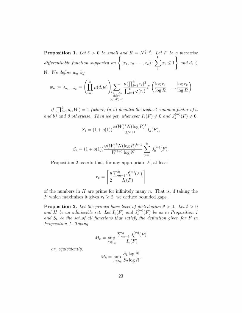
Proposition 1. Let δ > 0 be small and R = Nθ2−δ. Let F be a piecewise

differentiable function supported on

{(x1, x2, . . . , xk) :

k∑1

xi ≤ 1

}and di ∈

N. We define wn by

wn := λd1,...,dk =

(k∏

i=1

µ(di)di

)∑r1,...,rkdi|ri

(ri,W )=1

µ(∏k

i=1 ri)2∏k

i=1 ϕ(ri)F

(log r1logR

, . . . ,log rklogR

)

if (∏k

i=1 di,W ) = 1 (where, (a, b) denotes the highest common factor of a

and b) and 0 otherwise. Then we get, whenever Ik(F ) 6= 0 and J(m)k (F ) 6= 0,

S1 = (1 + o(1))ϕ(W )kN(logR)k

W k+1Ik(F ),

S2 = (1 + o(1))ϕ(W )kN(logR)k+1

W k+1 logN

k∑m=1

J(m)k (F ).

Proposition 2 asserts that, for any appropriate F , at least

rk =

⌈θ

2

∑km=1 J

(m)k (F )

Ik(F )

⌉

of the numbers in H are prime for infinitely many n. That is, if taking theF which maximises it gives rk ≥ 2, we deduce bounded gaps.

Proposition 2. Let the primes have level of distribution θ > 0. Let δ > 0and H be an admissible set. Let Ik(F ) and J

(m)k (F ) be as in Proposition 1

and Sk be the set of all functions that satisfy the definition given for F inProposition 1. Taking

Mk = supF∈Sk

∑km=1 J

(m)k (F )

Ik(F )

or, equivalently,

Mk = supF∈Sk

S1 logN

S2 logR,

23

then rk above becomes⌈θ2Mk

⌉and we have at least rk of n+hi are prime.

Explicitlylim infn→∞

(pn+rk − pn) ≤ max1≤i 6=j≤k

(hi − hj).

Our final proposition gives two explicit results for Mk and a generalbound.

Proposition 3. Let Mk be as in Proposition 2. We have:

1. 2 < M5

2. 4 < M105

3. log k − 2 log log k − 2 < Mk for sufficiently large k

We prove Proposition 2, assuming Proposition 1:

Proof. By the definition of Mk, there exists some F0 ∈ Sk such that

k∑1

J(m)k (F0) > (Mk − ε)Ik(F0).

As we said at the start of this section we’re looking to make S = S2 −mS1 > 0. By Proposition 1:

S = (1 + o(1))ϕ(W )kN(logR)k

W k+1

(logR

logN

k∑m=1

J(m)k (F0)−mIk(F0)

)

=ϕ(W )kN(logR)k

W k+1

(logR

logN

k∑m=1

J(m)k (F0)−mIk(F0) + o(1)

),

substituting Mk into S gives

≥ ϕ(W )kN(logR)k

W k+1Ik(F0)

((θ

2− ε

)(Mk − ε)−m+ o(1)

)≥ CN

(θMk

2− ε

(θ

2+Mk − ε

)− θMk

2+ δ + o(1)

)= CN

(ε2 − ε

θ

2− εMk + δ + o(1)

).

24

Then choosing ε < 12

δmax( θ

2,Mk)

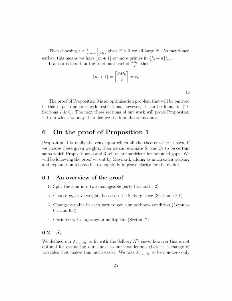
gives S > 0 for all large N . As mentioned

earlier, this means we have bm+ 1c or more primes in {hi + n}ki=1.If also δ is less than the fractional part of θMk

2, then

bm+ 1c =⌈θMk

2

⌉= rk

.

The proof of Proposition 3 is an optimisation problem that will be omittedin this paper due to length restrictions, however, it can be found in [11,Sections 7 & 8]. The next three sections of our work will prove Proposition1, from which we may then deduce the four theorems above.

6 On the proof of Proposition 1

Proposition 1 is really the crux upon which all the theorems lie: it says, ifwe choose these given weights, then we can evaluate S1 and S2 to be certainsums which Propositions 2 and 3 tell us are sufficient for bounded gaps. Wewill be following the proof set out by Maynard, adding as much extra workingand explanation as possible to hopefully improve clarity for the reader.

6.1 An overview of the proof

1. Split the sum into two manageable parts (5.1 and 5.2)

2. Choose wn sieve weights based on the Selberg sieve (Section 4.2.1)

3. Change variable in each part to get a smoothness condition (Lemmas6.1 and 6.3)

4. Optimise with Lagrangian multipliers (Section 7)

6.2 S1

We defined our λd1,...,dk to fit with the Selberg Λ2- sieve; however this is notoptimal for evaluating our sums, so our first lemma gives us a change ofvariables that makes this much easier. We take λd1,...,dk to be non-zero only

25

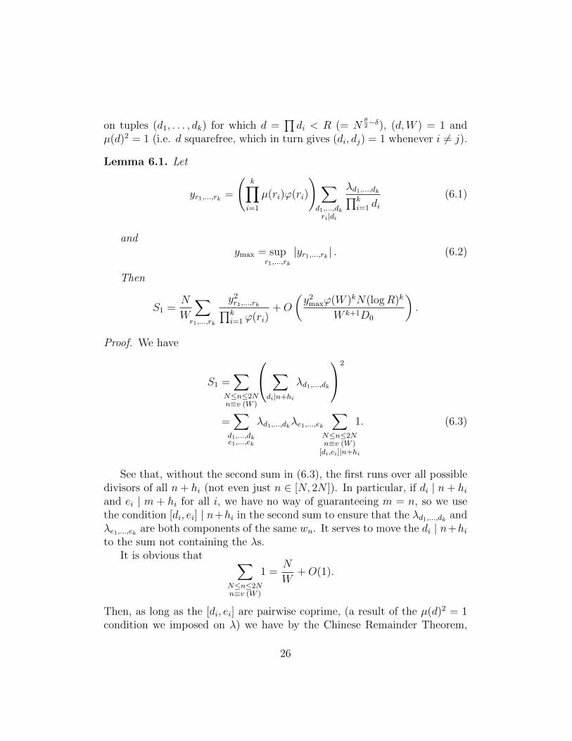
on tuples (d1, . . . , dk) for which d =∏

di < R (= Nθ2−δ), (d,W ) = 1 and

µ(d)2 = 1 (i.e. d squarefree, which in turn gives (di, dj) = 1 whenever i 6= j).

Lemma 6.1. Let

yr1,...,rk =

(k∏

i=1

µ(ri)ϕ(ri)

)∑d1,...,dkri|di

λd1,...,dk∏ki=1 di

(6.1)

andymax = sup

r1,...,rk

|yr1,...,rk | . (6.2)

Then

S1 =N

W

∑r1,...,rk

y2r1,...,rk∏ki=1 ϕ(ri)

+O

(y2maxϕ(W )kN(logR)k

W k+1D0

).

Proof. We have

S1 =∑

N≤n≤2Nn≡v (W )

∑di|n+hi

λd1,...,dk

2

=∑

d1,...,dke1,...,ek

λd1,...,dkλe1,...,ek

∑N≤n≤2Nn≡v (W )

[di,ei]|n+hi

1. (6.3)

See that, without the second sum in (6.3), the first runs over all possibledivisors of all n+ hi (not even just n ∈ [N, 2N ]). In particular, if di | n+ hi

and ei | m + hi for all i, we have no way of guaranteeing m = n, so we usethe condition [di, ei] | n+hi in the second sum to ensure that the λd1,...,dk andλe1,...,ek are both components of the same wn. It serves to move the di | n+hi

to the sum not containing the λs.It is obvious that ∑

N≤n≤2Nn≡v (W )

1 =N

W+O(1).

Then, as long as the [di, ei] are pairwise coprime, (a result of the µ(d)2 = 1condition we imposed on λ) we have by the Chinese Remainder Theorem,

26

for some v′ ∈{1, . . . ,W

∏ki=1[di, ei]

}:∑

N≤n≤2Nn≡v (W )

[di,ei]|n+hi

1 =∑

N≤n≤2N

n≡v′(W∏k

i=1[di,ei])

1

=N

W∏k

i=1[di, ei]+O(1), (6.4)

giving us

S1 =∑

d1,...,dke1,...,ek

W,[d1,e1],...,[dk,ek]pairwise coprime

λd1,...,dkλe1,...,ek

(N

W

1∏[di, ei]

+O(1)

). (6.5)

Simply for ease of notation, we let∑

denote summation with the

restriction W, [d1, e1], . . . , [dk, ek] pairwise coprime so that

S1 =N

W

∑d1,...,dke1,...,ek

λd1,...,dkλe1,...,ek∏[di, ei]

+O

( ∑d1,...,dke1,...,ek

|λd1,...,dkλe1,...,ek |

)(6.6)

We need to bound our error term so we can check it is not too large. Defineτr(n) as the number of ways of writing n as a product of r numbers; then,as with ymax in the statement of Lemma 6.1, take λmax = supd1,...,dk

|λd1,...,dk |and recall

∏ki=1 di < R, giving

∑|λd1,...,dkλe1,...,ek | � λ2

max × (number of terms in sum)

� λ2max

(∑d<R

τk(d)

)2

. (6.7)

Now we have to bound this sum; luckily for us, this is quite standard by firstusing Rankin’s trick ∑

d≤R

τk(d) ≤ R∑d≤R

τk(d)

d,

27

then splitting d into its prime factors,

= R∑

d1,...,dk∏di≤R

τk(∏k

i=1 di)∏ki=1 di

.

By definition τk(∏k

i=1 di) is 1 (as the di are squarefree and pairwise coprime),giving,

= R∑

d1,...,dk∏di≤R

1∏di,

and if we change∏

di ≤ R to just di ≤ R we get

≤ R

(∑d≤R

1

d

)k

� R(logR)k.

Putting it together we find

λ2max

(∑d<R

τk(d)

)2

� λ2maxR

2(logR)2k,

which will become negligible.We need to have λd1,...,dk and λe1,...,ek independent so that shortly we

can substitute them both out for the same term, however currently thereis a condition on [di, ei] in our summation, which necessarily introduces adependence. We shall remove this by using the fact that

1

[di, ei]=

1

diei

∑ui|di,ei

ϕ(ui).

28

Letting M be the main term of S1 this gives

M =N

W

∑d1,...,dke1,...,ek

λd1,...,dkλe1,...,ek

k∏i=1

1

diei

∑ui|di,ei

ϕ(ui)

=N

W

∑d1,...,dke1,...,ek

λd1,...,dkλe1,...,ek

∏(∑ui|di,ei ϕ(ui)

)(∏

di) (∏

ei)

=

N

W

∑u1,...,uk

(k∏

i=1

ϕ(ui)

) ∑d1,...,dke1,...,ekui|di,ei

(λd1,...,dkλe1,...,ek

(∏

di) (∏

ei)

). (6.8)

The last equality requires pulling out the ϕ(ui), changing the order ofoperations and changing the indexing. That’s quite a lot for one step, sowe’ll elucidate enough that you may believe it’s true. We’ll show how itworks for the case k = 2 and note that the method extends in a natural wayfor any k.

First notice that the only thing that changes is that the∏

(∑

ϕ(ui))

moves outside∑

and the condition ui|di, ei is added to the second sum, i.e.we may ignore (for the purpose of this exercise) the other summands. Take

σ =∑d1,d2

2∏i=1

∑ui|di

ϕ(ui).

This is a sum over all divisors ui of di, we’ll add an index to make this clear.Let Di = {ui,1, ui,2, . . . , ui,ni

} be the set of divisors of di, then a change toour new notation of ui,k (made in the first equality) gives

σ =∑d1,d2

2∏i=1

∑ui∈Di

ϕ(ui) =∑d1,d2

2∏i=1

ni∑j=1

ϕ(ui,j)

=∑d1,d2

(ni∑j=1

ϕ(u1,j)

)(ni∑k=1

ϕ(u2,k)

)

29

=∑d1,d2

ϕ(u1,1)ϕ(u2,1) + · · ·+ ϕ(u1,n1)ϕ(u2,1) + · · ·+ ϕ(u1,n1)ϕ(u2,n2)

=∑d1,d2

∑1≤j≤n11≤k≤n2

ϕ(u1,j)ϕ(u2,k)

=∑d1,d2

∑ui,j∈Di

2∏k=1

ϕ(uk,j).

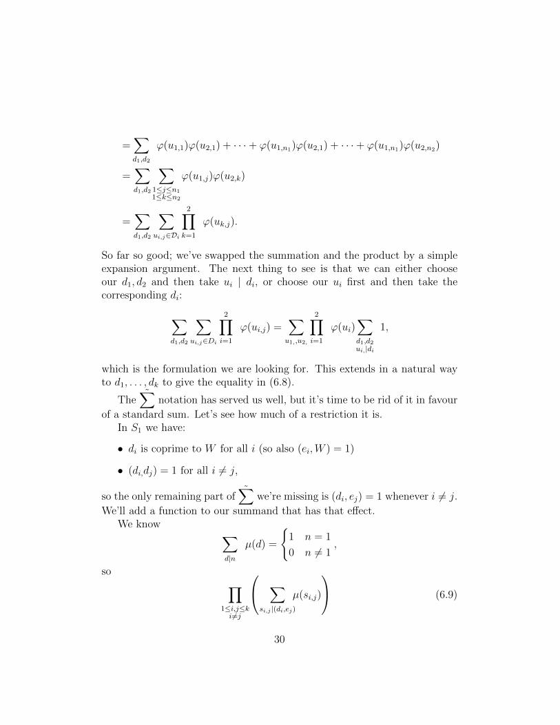
So far so good; we’ve swapped the summation and the product by a simpleexpansion argument. The next thing to see is that we can either chooseour d1, d2 and then take ui | di, or choose our ui first and then take thecorresponding di:∑

d1,d2

∑ui,j∈Di

2∏i=1

ϕ(ui,j) =∑u1,,u2,

2∏i=1

ϕ(ui)∑d1,d2ui,|di

1,

which is the formulation we are looking for. This extends in a natural wayto d1, . . . , dk to give the equality in (6.8).

The∑

notation has served us well, but it’s time to be rid of it in favour

of a standard sum. Let’s see how much of a restriction it is.In S1 we have:

• di is coprime to W for all i (so also (ei,W ) = 1)

• (di,dj) = 1 for all i 6= j,

so the only remaining part of∑

we’re missing is (di, ej) = 1 whenever i 6= j.

We’ll add a function to our summand that has that effect.We know ∑

d|n

µ(d) =

{1 n = 1

0 n 6= 1,

so ∏1≤i,j≤k

i 6=j

∑si,j |(di,ej)

µ(si,j)

(6.9)

30

is equivalent to the additional condition (as if any (di, ej) 6= 1 then the wholeproduct becomes 0). This gives

M =N

W

∑u1,...,uk

(k∏

i=1

ϕ(ui)

)∑d1,...,dke1,...,ekui|di,ei

λd1,...,dkλe1,...,ek

(∏

di) (∏

ei)

∏1≤i,j≤k

i 6=j

∑si,j |(di,ej)

µ(si,j)

(6.10)and then, as with ϕ, we can take this product outside to get

S1 =N

W

∑u1,...,uk

(k∏

i=1

ϕ(ui)

) ∑1≤i,j≤k

i 6=j

( ∏1≤i,j≤k

i 6=j

µ(si,j)

) ∑d1,...,dke1,...,ekui|di,ei

si,j |di,ej ,∀i 6=j

(λd1,...,dkλe1,...,ek

(∏

di) (∏

ei)

).

(6.11)Here we go now - the part you’ve all been waiting for - it’s time to

introduce a change of variables. Let

yr1,...,rk =

(k∏

i=1

µ(ri)ϕ(ri)

)∑d1,...,dkri|di

λd1,...,dk∏ki=1 di

. (6.12)

Then any yr1,...,rk satisfying similar conditions to those we have on λd1,...,dk

(specifically: r =∏k

i=1 ri < R, (r,W ) = 1 and µ(r)2 = 1) corresponds to aλd1,...,dk that fulfils our requirements because the change is invertible (whichwe will now show):

yr1,...,rk∏ϕ(ri)

=k∏

i=1

µ(ri)∑

d1,...,dkri|di

λd1,...,dk∏ki=1 di

∑r1,...,rkei|ri

yr1,...,rk∏ϕ(ri)

=∑

r1,...,rkei|ri

k∏i=1

µ(ri)∑

d1,...,dkri|di

λd1,...,dk∏ki=1 di

=∑

r1,...,rkei|riri|di

k∏i=1

µ(ri)∑

d1,...,dk

λd1,...,dk∏ki=1 di

. (6.13)

31

We need to do a bit more manipulation using properties of the Mobiusfunction to get this in an accessible form. As each ei, ri, di triple isindependent, we can just show how this works with a single variable andit extends very easily to the product.

Taking ∑ri

ei|riri|di

µ(ri)

set ri = eir′i, then using that ri is squarefree, we can split up µ(ri) into

µ(r′i)µ(ei) and the sum becomes

=∑r′i|

diei

µ(r′i)µ(ei)

= µ(ei)∑r′i|

diei

µ(r′i).

But this sum is zero if diei

is not 1, so

=

{µ(ei) di = ei

0 di 6= ei

which, in turn, thanks to our joint ei | ri and ri | di conditions, gives thatei = di whenever this sum is non-zero, so we get that (6.12) becomes

k∏i=1

µ(ei)∑

e1,...,ek

λe1,...,ek∏ki=1 ei

.

The ei have been prescribed by the di so we can also remove the sum overall ei to get

=λe1,...,ek

∏ki=1 µ(ei)∏k

i=1 ei.

But µ(x)2 = 1 whenever µ(x) is not zero, so every time it contributes tothe sum it is also a self inverse, that is, µ(x) = 1

µ(x), which we substitute in

mostly for convenience of the notation:∑r1,...,rkei|ri

yr1,...,rk∏ϕ(ri)

=λe1,...,ek∏ki=1 µ(ei)ei

. (6.14)

32

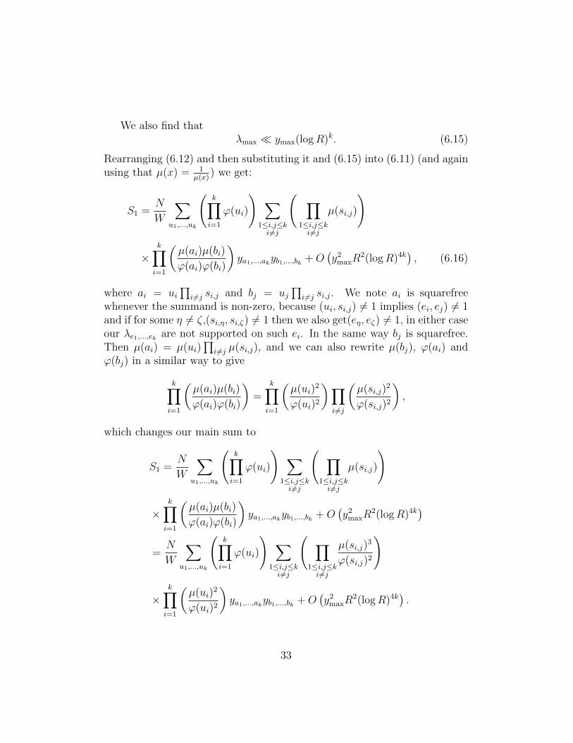
We also find thatλmax � ymax(logR)k. (6.15)

Rearranging (6.12) and then substituting it and (6.15) into (6.11) (and againusing that µ(x) = 1

µ(x)) we get:

S1 =N

W

∑u1,...,uk

(k∏

i=1

ϕ(ui)

) ∑1≤i,j≤k

i 6=j

( ∏1≤i,j≤k

i 6=j

µ(si,j)

)

×k∏

i=1

(µ(ai)µ(bi)

ϕ(ai)ϕ(bi)

)ya1,...,akyb1,...,bk +O

(y2maxR

2(logR)4k), (6.16)

where ai = ui

∏i 6=j si,j and bj = uj

∏i 6=j si,j. We note ai is squarefree

whenever the summand is non-zero, because (ui, si,j) 6= 1 implies (ei, ej) 6= 1and if for some η 6= ζ,(si,η, si,ζ) 6= 1 then we also get(eη, eζ) 6= 1, in either caseour λe1,...,ek are not supported on such ei. In the same way bj is squarefree.Then µ(ai) = µ(ui)

∏i 6=j µ(si,j), and we can also rewrite µ(bj), ϕ(ai) and

ϕ(bj) in a similar way to give

k∏i=1

(µ(ai)µ(bi)

ϕ(ai)ϕ(bi)

)=

k∏i=1

(µ(ui)

2

ϕ(ui)2

)∏i 6=j

(µ(si,j)

2

ϕ(si,j)2

),

which changes our main sum to

S1 =N

W

∑u1,...,uk

(k∏

i=1

ϕ(ui)

) ∑1≤i,j≤k

i 6=j

( ∏1≤i,j≤k

i 6=j

µ(si,j)

)

×k∏

i=1

(µ(ai)µ(bi)

ϕ(ai)ϕ(bi)

)ya1,...,akyb1,...,bk +O

(y2maxR

2(logR)4k)

=N

W

∑u1,...,uk

(k∏

i=1

ϕ(ui)

) ∑1≤i,j≤k

i 6=j

( ∏1≤i,j≤k

i 6=j

µ(si,j)3

ϕ(si,j)2

)

×k∏

i=1

(µ(ui)

2

ϕ(ui)2

)ya1,...,akyb1,...,bk +O

(y2maxR

2(logR)4k).

33

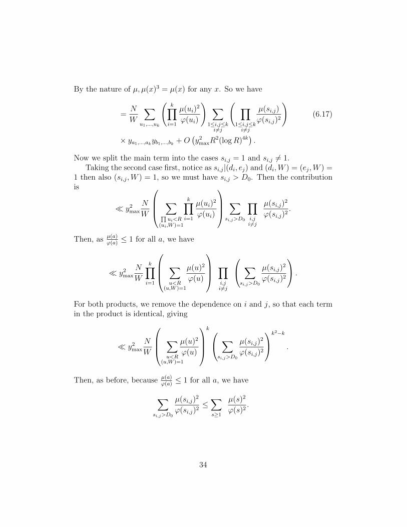
By the nature of µ, µ(x)3 = µ(x) for any x. So we have

=N

W

∑u1,...,uk

(k∏

i=1

µ(ui)2

ϕ(ui)

) ∑1≤i,j≤k

i 6=j

( ∏1≤i,j≤k

i 6=j

µ(si,j)

ϕ(si,j)2

)(6.17)

× ya1,...,akyb1,...,bk +O(y2maxR

2(logR)4k).

Now we split the main term into the cases si,j = 1 and si,j 6= 1.Taking the second case first, notice as si,j|(di, ej) and (di,W ) = (ej,W ) =

1 then also (si,j,W ) = 1, so we must have si,j > D0. Then the contributionis

� y2max

N

W

∑∏

ui<R(ui,W )=1

k∏i=1

µ(ui)2

ϕ(ui)

∑si,j>D0

∏i,ji 6=j

µ(si,j)2

ϕ(si,j)2.

Then, as µ(a)ϕ(a)

≤ 1 for all a, we have

� y2max

N

W

k∏i=1

∑u<R

(u,W )=1

µ(u)2

ϕ(u)

∏i,ji 6=j

∑si,j>D0

µ(si,j)2

ϕ(si,j)2

.

For both products, we remove the dependence on i and j, so that each termin the product is identical, giving

� y2max

N

W

∑u<R

(u,W )=1

µ(u)2

ϕ(u)

k ∑

si,j>D0

µ(si,j)2

ϕ(si,j)2

k2−k

.

Then, as before, because µ(a)ϕ(a)

≤ 1 for all a, we have

∑si,j>D0

µ(si,j)2

ϕ(si,j)2≤∑s≥1

µ(s)2

ϕ(s)2.

34

We can take k2 − k − 1 terms out of our second sum and apply thisinequality to give:

� y2max

N

W

∑u<R

(u,W )=1

µ(u)2

ϕ(u)

k ∑

si,j>D0

µ(si,j)2

ϕ(si,j)2

(∑s≥1

µ(s)2

ϕ(s)2

)k2−k−1

.

(6.18)For the result we need to bound each part in this sum. We’re going to workfrom the last factor to the first.

We recall that ϕ(s) ≈ s, particularly for large s. So heuristically we get∑s≥1

µ(s)2

ϕ(s)2≈∑s≥1

1

s2=

π2

6.

As the right hand side converges to a constant, so does the left.Next, we’re taking exactly the same sum, but starting a little further

along: ∑si,j>D0

µ(si,j)2

ϕ(si,j)2≈∑s≥D0

1

s2

=∑s≥1

1

s2−

D0∑s=1

1

s2

=π2

6+∑n≥1

(−1)n

n!Dn0

≈ π2

6− 1

D0

=C

D0

,

for a constant C which will be absorbed into our � constant.Finally, we have just one term left:∑

u<R(u,W )=1

µ(u)2

ϕ(u).

However we’re going to need an additional lemma to bound this:

35

Lemma 6.2. Let U1, U2, L > 0. Let γ be a multiplicative function satisfying

0 ≤ γ(p)

p≤ 1− U1,

and

−L ≤∑

w≤p≤z

γ(p) log p

p− log

z

w≤ U2

for any 2 ≤ w ≤ z. Let η be the totally multiplicative function defined onprimes by

η(p) =γ(p)

p− γ(p).

Finally, let G : [0, 1] → R be smooth, and let Gmax =supt∈[0,1] (|G(t)|+ |G′(t)|). Then

∑d<z

µ(d)2η(d)G

(log d

log z

)= P log z

ˆ 1

0

G(x) dx+OU1,U2(PLGmax)

where

P =∏

p prime

(1− γ(p)

p

)−1(1− 1

p

).

Proof. As we’re only going to use this as a tool, the proof is not veryenlightening. However, it can be found in [5, Lemmas 3 & 4].

Getting back to bounding, we rewrite∑u<R

(u,W )=1

µ(u)2

ϕ(u),

so that the lemma is clearly applicable. Take

γ(p) =

{1 p - W0 p | W

andG(x) = 1.

36

Then ∑d<z

µ(d)2η(d)G

(log d

log z

)=∑d<z

µ(d)2∏p|d

γ(p)

p− γ(p)

=∑d<z

(d,W )=1

µ(d)2∏p|d(p− 1)

=∑d<R

(d,W )=1

µ(d)2

ϕ(d), (6.19)

which is exactly as we’d like. So to get our bound we just have to evaluateP for this γ (as the integral is trivially 1). We have(

1− γ(p)

p

)=

{(1− 1

p

)p - W

1 p | W,

so

P =∏p|W

(1− 1

p

)=∏p|W

(p− 1)(∏p|W

p)−1

=ϕ(W )

W, (6.20)

giving us the bound ∑u<R

(u,W )=1

µ(u)2

ϕ(u)

=ϕ(W )

Wlog(R) +O

(ϕ(W )

W

)(6.21)

=ϕ(W )

W(log(R) +O(1)) .

but as this is an error term itself, the O(1) will disappear in the final error.

37

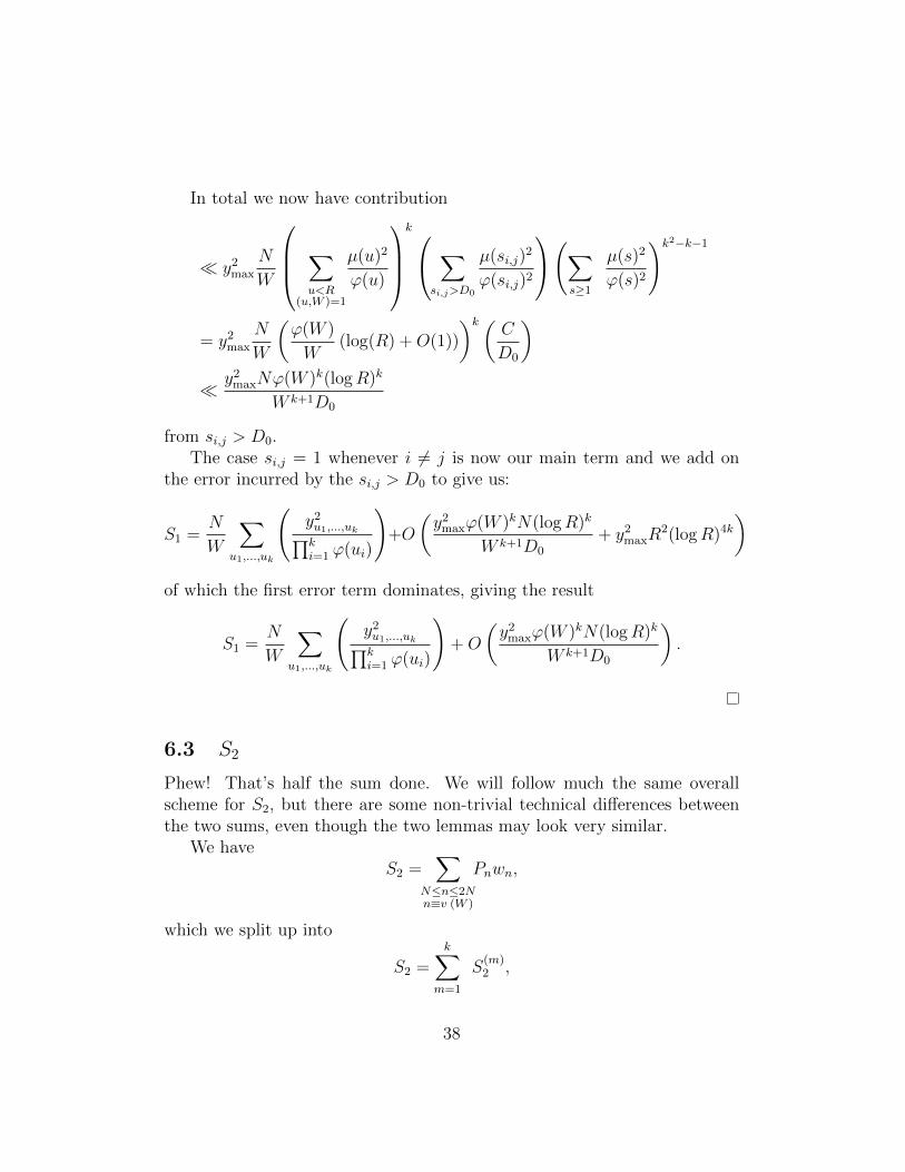
In total we now have contribution

� y2max

N

W

∑u<R

(u,W )=1

µ(u)2

ϕ(u)

k ∑

si,j>D0

µ(si,j)2

ϕ(si,j)2

(∑s≥1

µ(s)2

ϕ(s)2

)k2−k−1

= y2max

N

W

(ϕ(W )

W(log(R) +O(1))

)k (C

D0

)� y2maxNϕ(W )k(logR)k

W k+1D0

from si,j > D0.The case si,j = 1 whenever i 6= j is now our main term and we add on

the error incurred by the si,j > D0 to give us:

S1 =N

W

∑u1,...,uk

(y2u1,...,uk∏ki=1 ϕ(ui)

)+O

(y2maxϕ(W )kN(logR)k

W k+1D0

+ y2maxR2(logR)4k

)of which the first error term dominates, giving the result

S1 =N

W

∑u1,...,uk

(y2u1,...,uk∏ki=1 ϕ(ui)

)+O

(y2maxϕ(W )kN(logR)k

W k+1D0

).

6.3 S2

Phew! That’s half the sum done. We will follow much the same overallscheme for S2, but there are some non-trivial technical differences betweenthe two sums, even though the two lemmas may look very similar.

We haveS2 =

∑N≤n≤2Nn≡v (W )

Pnwn,

which we split up into

S2 =k∑

m=1

S(m)2 ,

38

where

S(m)2 =

∑N≤n≤2Nn≡v (W )

χP (n+ hm)

( ∑d1,...,dkdi|n+hi

λd1,...,dk

)2

.

Now we have the equivalent of Lemma 6.1 for S(m)2 .

Define g(x) to be the multiplicative function defined on the primes byg(p) = p− 2 and analogously to (6.2), define

y(m)max = sup

r1,...,rk

∣∣y(m)r

∣∣ .Lemma 6.3. Let

y(m)r =

(k∏

i=1

µ(ri)g(ri)

) ∑d1,...,dkri|didm=1

λd∏ki=1 ϕ(di)

. (6.22)

Then for any A > 0

S(m)2 =

N

ϕ(W ) logN

∑r1,...,rk

(y(m)r )2∏k

i=1 g(ri)+O

((y

(m)max)2ϕ(W )k−2N(logR)k−2

W k−1D0

)

+O

(y2maxN

(logN)A

). (6.23)

Proof. Recall that we use [a, b] to refer to the lowest common multiple of aand b.

In the same way as with S1, we change the order of summation to putthe λd in a sum just depending on d1, . . . , dk and e1, . . . , ek:

S(m)2 =

∑d1,...,dke1,...,ek

λd1,...,dkλe1,...,ek

∑N≤n≤2Nn≡v (W )

[di,ei]|n+hi

χP (n+ hm).

Again, we look at the inner sum first, although this time its expansion isnot quite so obvious (we’ll explain it after setting it all out).

Defineq := W

∏[di, ei],

39

then∑N≤n≤2Nn≡v (W )

[di,ei]|n+hi

χP (n+ hm)

=∑

N≤n≤2N

χp(n)

ϕ(q)+O

1 + sup(a,q)=1

∣∣∣∣∣∣∣∣∑

N≤n≤2Nn≡a (q)

χp(n)−1

ϕ(q)

∑N≤n≤2N

χp(n)

∣∣∣∣∣∣∣∣ .

For ease of notation, we’ll set

XN =∑

N≤n≤2N

χp(n)

and

E(N, q) = O

1 + sup(a,q)=1

∣∣∣∣∣∣∣∣∑

N≤n≤2Nn≡a (q)

χp(n)−1

ϕ(q)

∑N≤n≤2N

χp(n)

∣∣∣∣∣∣∣∣ . (6.24)

Let’s look at each part of this separately.We’re looking for the number of elements in {n+ hm}2Nn=N that are prime,

congruent to v modulo W , and coprime to∏[di, ei]. We can immediately

remove the hm from the χp function incurring an error of at most 1 whichwe included in the E(N, q) term. The number of elements that satisfy ourcongruence conditions is N

ϕ(q)+O(1), where, in this case, O(1) actually means

±1 or 0. The number of those which we expect to be prime is then

1

ϕ(q)

∑N≤n≤2N

χp(n) +O(1),

but unfortunately this is not sufficient when dealing with primes. The primenumbers may not be evenly distributed among the congruence classes of q,and this means we have to add an extra error term, the second part of ourE(N, q) definition. This part says we’ll be wrong by at most the largestdifference between what we expect to be true and what is actually true.

40

Now using the∑

notation as before (summing only over cases when

W, [d1, e1], . . . , [dk, ek] are all pairwise coprime) we have

S(m)2 =

Xn

ϕ(W )

∑d1,...,dke1,...,ek

dm=em=1

λd1,...,dkλe1,...,ek

ϕ(∏[di, ei])

+O

( ∑d1,...,dke1,...,ek

λ2maxE(N, q)

).

Following our treatment of S1, we’ll bound the error first, using the samebound of λmax � ymax(logR)k. A cautious reader may worry that the slight(‘slight’ because if n has no small factors then ϕ(n) ≈ n ≈

∏p|n p−2 = g(n))

change in our definition of y with g(ri) in place of ϕ(ri) will change thisbound, but that change is held in the ymax part of the bound. The otherthing we want to bound is

∑d1,...,dke1,...,ek

E(N, q) =∑

d1,...,dke1,...,ek

E(N,Wk∏

i=1

[di, ei)])

=∑q

E(N, q){# of different di, eiwith

∏[di, ei] =

q

W

}.

As λd are only non-zero when∏

di ≤ R, we have that q ≤ R2W . The diwere defined to be squarefree and W clearly is by its definition, so we onlyneed to consider squarefree q in this range.

Lemma 6.4. For any square-free integer n, there are τ3k(n) choices ford1, . . . , dk, e1, . . . , ek such that W

∏ki=1[di, ei] = n.

Proof. As n is square-free, given p | n, we see that if p | W , then p - di andp - ei for any i

If instead, p | n and p - W then we must choose one of k pairs di, ei suchthat p | [di, ei]. Then we choose one of 3 options:

p | di p - ei,p - di p | ei,p | di p | ei.

41

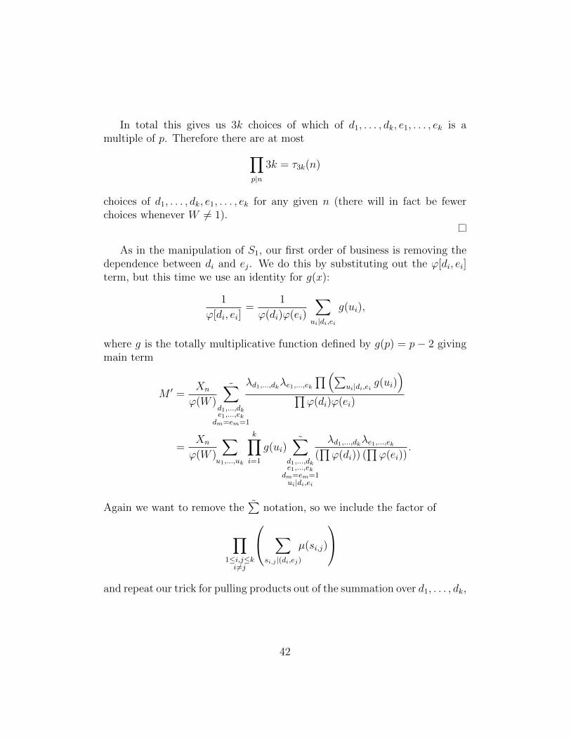
In total this gives us 3k choices of which of d1, . . . , dk, e1, . . . , ek is amultiple of p. Therefore there are at most∏

p|n

3k = τ3k(n)

choices of d1, . . . , dk, e1, . . . , ek for any given n (there will in fact be fewerchoices whenever W 6= 1).

As in the manipulation of S1, our first order of business is removing thedependence between di and ej. We do this by substituting out the ϕ[di, ei]term, but this time we use an identity for g(x):

1

ϕ[di, ei]=

1

ϕ(di)ϕ(ei)

∑ui|di,ei

g(ui),

where g is the totally multiplicative function defined by g(p) = p− 2 givingmain term

M ′ =Xn

ϕ(W )

∑d1,...,dke1,...,ek

dm=em=1

λd1,...,dkλe1,...,ek

∏(∑ui|di,ei g(ui)

)∏

ϕ(di)ϕ(ei)

=Xn

ϕ(W )

∑u1,...,uk

k∏i=1

g(ui)∑

d1,...,dke1,...,ek

dm=em=1ui|di,ei

λd1,...,dkλe1,...,ek

(∏

ϕ(di)) (∏

ϕ(ei)).

Again we want to remove the∑

notation, so we include the factor of

∏1≤i,j≤k

i 6=j

∑si,j |(di,ej)

µ(si,j)

and repeat our trick for pulling products out of the summation over d1, . . . , dk,

42

e1, . . . , ek to give us

M ′ =Xn

ϕ(W )

∑u1,...,uk

(k∏

i=1

g(ui)

) ∑1≤i,j≤k

i 6=j

( ∏1≤i,j≤k

i 6=j

µ(si,j)

)

×∑

d1,...,dke1,...,ek

dm=em=1ui|di,ei

si,j |di,ej ,∀i 6=j

(λd1,...,dkλe1,...,ek

(∏

ϕ(di)) (∏

ϕ(ei))

).

If you’ve been comparing to Section 6.1 you’ll know what’s coming next, withjust a slight adjustment to cater for the g(ui) in place of ϕ(ui). We make thesubstitution

y(m)r1,...,rk

=

(k∏

i=1

µ(ri)g(ri)

) ∑d1,...,dkri|didm=1

λd1,...,dk∏ki=1 ϕ(di)

(6.25)

which gives us

M ′ =Xn

ϕ(W )

∑u1,...,uk

(k∏

i=1

g(ui)

) ∑1≤i,j≤k

i 6=j

( ∏1≤i,j≤k

i 6=j

µ(si,j)

)

×k∏

i=1

(µ(ai)µ(bi)

g(ai)g(bi)

)y(m)a1,...,ak

y(m)b1,...,bk

=Xn

ϕ(W )

∑u1,...,uk

(k∏

i=1

µ(ui)2

g(ui)

) ∑1≤i,j≤k

i 6=j

( ∏1≤i,j≤k

i 6=j

µ(si,j)3

g(si,j)2

)y(m)a1,...,ak

y(m)b1,...,bk

=Xn

ϕ(W )

∑u1,...,uk

(k∏

i=1

µ(ui)2

g(ui)

) ∑1≤i,j≤k

i 6=j

( ∏1≤i,j≤k

i 6=j

µ(si,j)

g(si,j)2

)y(m)a1,...,ak

y(m)b1,...,bk

,

with ai = ui

∏i 6=j si,j and bj = uj

∏i 6=j si,j as before. Then we split into the

cases for si,j > D0 and si,j = 1. We follow an identical method to get an

43

analogous result to (6.18), this time with g(u) in place of ϕ(u):

(y(m)max

)2 Xn

ϕ(W )

∑u<R

(u,W )=1

µ(u)2

g(u)

k−1 ∑

si,j>D0

µ(si,j)2

g(si,j)2

(∑s≥1

µ(s)2

g(s)2

)k2−k−1

.

(6.26)Then we bound the sums as before, along with estimating Xn to be N

log N, to

get

�(y(m)max

)2 N

ϕ(W ) logN

(ϕ(W ) logR

W

)k−11

D0

=(y(m)max

)2 ϕ(W )k−2N (logR)k−1

W k−1D logN.

Thus we get the result that

S(m)2 =

Xn

ϕ(W )

∑u1,...,uk

(k∏

i=1

g(ui)

)yu1,...,uk

+O

((y(m)max

)2 ϕ(W )k−2N (logR)k−1

W k−1D logN

).

7 The Lagrangian Method

Our aim is to make the value of S1 as small as possible while making S2

large. This idea of minimising with a constraint suggests using the methodof Lagrangian multipliers, which is exactly what we do now.

Taking just the main terms, we have

S1 =N

W

∑r1,...,rk

y2r1,...,rk∏ki=1 ϕ(ri)

,

S2 =k∑

m=1

N

ϕ(W ) logN

∑r1,...,rk

(y(m)r )2∏k

i=1 g(ri).

There are two tricks we can use right from the start: first we can drop allconstants because it won’t affect which choices of yr are minimal; second, we

44

note that scaling S1 scales S2 an equivalent amount so we can set∑r1,...,rk

y2r1,...,rk∏ki=1 ϕ(ri)

= 1,

and this will be our constraint for the Lagrangian multipliers method.

L(y, λ) = S2 − λ (S1 − 1)

L(y, λ) =k∑

m=1

∑r1,...,rk

(y(m)r1,...,rk)

2∏g(ri)

− λ

( ∑r1,...,rk

y2r1,...,rk∏ϕ(ri)

− 1

). (7.1)

So the system of equations we are trying to solve is:

∂L

∂yu1,...,uk

= 0

∂y(m)r1,...,rk

∂yu1,...,uk

= 0.

For both of these equations we have to be clear on how y(m)r depends on

yu1,...,ukand so solving the second one gets us a long way towards solving the

first. Recall the definitions of y(m)r and yu:

y(m)r =

(k∏

i=1

µ(ri)g(ri)

)∑d1,...,dkri|didm=1

λd∏ki=1 ϕ(di)

yu =

(k∏

i=1

µ(ui)ϕ(ui)

)∑d1,...,dkui|di

λd∏ki=1 di

.

To evaluate∂y

(m)r1,...,rk

∂yu1,...,uk, it is necessary for us to have an expression for y

(m)r in

terms of yu; we shall get this with the following lemma.

Lemma 7.1. If rm = 1 then

y(m)r1,...,rk

=∑am

yr1,...,rm−1,am,rm+1,...,rk

ϕ(am)+O

(ymaxϕ(W ) logR

WD0

). (7.2)

45

Proof. Assume rm = 1. Then, from (6.14), we have∑r1,...,rkdi|ri

yr1,...,rk∏ϕ(ri)

=λd1,...,dk∏ki=1 µ(di)di

and from (6.22),

y(m)r =

(k∏

i=1

µ(ri)g(ri)

) ∑d1,...,dkri|didm=1

λd∏ki=1 ϕ(di)

.

A moment of care must be taken here to clarify that the vectors r are dummyvariables and not the same in the two definitions, henceforth we change theyr to ya to avoid confusion. Now substituting for λd we get

y(m)r =

(k∏

i=1

µ(ri)g(ri)

) ∑d1,...,dkri|didm=1

∏ki=1 µ(di)di∏ki=1 ϕ(di)

∑a1,...,akdi|ai

ya∏ki=1 ϕ(ai)

. (7.3)

We want to swap the order of the summations to get them into forms we canevaluate. Currently, we choose ri first, then di and finally choose the ai suchthat di | ai; instead, we want to choose the ai before the di while keeping allother conditions the same.

As we have ri | di and di | ai, we have ri | ai and having selected the ai wecan then keep the di | ai condition by imposing it on the second sum, givingus

y(m)r =

(k∏

i=1

µ(ri)g(ri)

) ∑a1,...,akri|ai

ya∏ki=1 ϕ(ai)

∑d1,...,dk

ri|di, di|aidm=1

k∏i=1

µ(di)diϕ(di)

.

By the multiplicative nature of µ and ϕ, this is

y(m)r =

(k∏

i=1

µ(ri)g(ri)

) ∑a1,...,akri|ai

ya∏ki=1 ϕ(ai)

∏i 6=m

µ(ai)riϕ(ai)

. (7.4)

We note that ya is 0 whenever (aj,W ) 6= 1 so either aj = rj or aj > D0rj.

46

As for (6.17), we will take aj > D0rj first and show it has negligibleimpact. The sum (7.4) with the caveat aj > D0rj is less than a constanttimes: (

k∏i=1

µ(ri)g(ri)

) ∑a1,...,akri|ai

ymax∏ki=1 ϕ(ai)

∏i 6=j

µ(ai)riϕ(ai)

. (7.5)

Previously, we chose ri first, then subsequently the corresponding ai, andthen take a product over all the ϕ(ai). This means that when we make theai conditions separate we have to square the product to compensate for thisdouble counting. We do this, as well as splitting the sum into i = m andi 6= m summands, to get:

� ymax

(k∏

i=1

g(ri)ri

)( ∑a1,...,ak

µ(am)2

ϕ(am)

) ∑a1,...,aki 6=m

µ(ai)2

ϕ(ai)2

∑a1,...,ak

∏i 6=jri|ai

µ(ai)2

ϕ(ai)2

� ymax

(k∏

i=1

g(ri)ri

) ∑am<R

(am,W )=1

µ(am)2

ϕ(am)

( ∑

ai>D0

µ(ai)2

ϕ(ai)2

)∏i 6=ji 6=m

∑ai>D0ri|ai

µ(ai)2

ϕ(ai)2

,

each part of which we can evaluate as we did for (6.17), leaving us with

� ymax

(k∏

i=1

g(ri)riϕ(ri)2

)ϕ(W ) logR

WD0

� ymaxϕ(W ) logR

WD0

. (7.6)

47

This gives us that the main term is when aj = rj for all j 6= m and so

y(m)r =

(k∏

i=1

µ(ri)g(ri)

)∑am

(yr1,...,rm−1,am,rm+1,...,rk∏k

i=1 ϕ(ai)

)∏i 6=m

µ(ai)riϕ(ai)

+O

(ymax

ϕ(W ) logR

WD0

)=

(k∏

i=1

µ(ri)g(ri)

ϕ(ri)

)∑am

(yr1,...,rm−1,am,rm+1,...,rk

ϕ(am)

)∏i 6=m

µ(ri)riϕ(ri)

+O

(ymax

ϕ(W ) logR

WD0

)=

(k∏

i=1

µ(ri)2g(ri)ri

ϕ(ri)2

)∑am

(yr1,...,rm−1,am,rm+1,...,rk

ϕ(am)

)ϕ(am)

2

µ(am)am

+O

(ymax

ϕ(W ) logR

WD0

).

Finally we note thatg(x)x

ϕ(x)2= 1 +O(x−2).

As our y(m)r are only supported when

∏ki=1 ri > D0, this can be compensated

for with a1 +O(D−2

0 )

term. This is still less than our other error term. Finally, we see that both yrand y

(m)r are zero when the ri are not square free, so we can drop the µ(ri)

2

term to get

y(m)r1,...,rk

=∑am

yr1,...,rm−1,am,rm+1,...,rk

ϕ(am)+O

(ymaxϕ(W ) logR

WD0

).

As a result of this lemma, we have that y(m)r is a sum of terms almost all

of which do not depend on yu. For dependence on yu we need ri = ui for alli 6= m; in which case, the previous lemma gives, for rm = 1,

y(m)r =

∑am

yr1,...,rm−1,am,rm+1,...,rk

ϕ(am)+O

(ymaxϕ(W ) logR

WD0

). (7.7)

48

Hence,

∂y(m)r

∂yu=

∑am

1ϕ(am)

, if ri = ui for all i 6= m

0, otherwise. (7.8)

Which gives in total for L

∂L

∂yu1,...,uk

=∂

∂yu

k∑m=1

∑r1,...,rk

(y(m)r )2∏g(ri)

− λ∂

∂yu

( ∑r1,...,rk

y2r∏ϕ(ri)

)

=k∑

m=1

∑r1,...,rk

2∂(y

(m)r )

∂yu

y(m)r∏g(ri)

− λ

( ∑r1,...,rk

2∂yr∂yu

yr∏ϕ(ri)

).

The sum over the ri has all terms 0 except for when the ri = ui, i 6= m, sowe can remove this sum and instead evaluate

k∑m=1

1∏i 6=m

g(ui)

∑am

2y(m)u1,...,um−1,am,um+1,...,uk

ϕ(am)− λ

(2

yu∏ϕ(ui)

).

Then, setting the equation to be zero, we get

λyu =∏

ϕ(ui)k∑

m=1

1∏i 6=m

g(ui)

∑am

y(m)u1,...,um−1,am,um+1,...,uk

ϕ(am)

and, by a slight modification of (7.7), we get

=∏

ϕ(ui)k∑

m=1

1∏i 6=m

g(ui)

y(m)u1,...,um−1,1,um+1,...,uk

ϕ(um).

Note also thatk∑

i=1

1∏i 6=m g(ui)

=

∑ki=1 g(ui)∏ki=1 g(ui)

and substituting this in gives us a condition on yu:

λyu =k∏

i=1

ϕ(ui)

g(ui)

k∑m=1

g(um)

ϕ(um)y(m)u1,...,um−1,1,um+1,...,uk

. (7.9)

49

8 Smooth choice of y

As a result of the previous section we have the condition

λyr =

(k∏

i=1

ϕ(ri)

g(ri)

)k∑

m=1

g(rm)

ϕ(rm)y(m)r1,...,rm−1,1,rm+1,...,rk

but this is very easily simplified by the condition we made in Section 5.2:that all our weights would be coprime to W .

First, it is quite intuitive that g(x) will be ‘close’ to x for x with onlylarge prime factors pi because

pi−1pi

→ 1 as pi increases. In fact, ϕ(x) willbe even closer to x in light of the fact that for any repeated prime p in thefactorisation of x, g(pk) contributes (p− 1)k to g(x) whereas ϕ(pk) providesa factor of pk−1(p − 1) (and for the squarefree factors of x we have ϕ(x) =∏

ϕ(pi) =∏(pi − 1) = g(x)) meaning we can make the estimation ϕ(x)

g(x)≈ 1

and thus

λyr ≈k∑

m=1

y(m)r1,...,rm−1,1,rm+1,...,rk

. (8.1)

Before we studied the yr, it would have been reasonable to suggest thatsolutions might depend on the prime factorisation of yr. What the aboveequation gives us, is that this is not the case, and instead we have transformedour number theoretic problem into something that looks like a functionalanalysis question. This incentivises us to try using a smooth2 function as ouryr and see how it works out. In this case, we choose

yr = F

(log r1logR

, . . . ,log rklogR

). (8.2)

Of course, for this statement to stand a chance of being useful, our functionF has to take into account all the requirements we placed on our yr, fromProposition 1. Hence we set F to be 0 whenever:

1. r =∏k

i=1 rk satisfies either (r,W ) > 1 or µ(r) 6= 1.

2.∑k

i=1 ri > 1 (i.e. we need r in the unit ball of Rk in the ‖.‖1−norm).

2The word ‘smooth’ is very oversubscribed in mathematics. In number theory itdescribes the prime factors of a number, but here, we’ve moved on from number theoryto functional analysis. Now we use ‘smooth’ to mean having continuous derivative almosteverywhere.

50

We impose the second condition because we plan to consider when R is verylarge and it’s neater to remove the dependence on R in the domain. It isthen done by scaling by logR every argument of F which makes the domainof F [0, 1]k (recall from Section 5.2 we have

∏ri < R).

Finally, we can reach the conclusion that the last two sections have beenleading us towards: the evaluations of S1 and S2 given in Proposition 1. We’llbegin with S1.

Lemma 8.1. Let yr be given as in (8.2) for a smooth function F . Let

Fmax = sup(t1,...,tk)∈[0,1]k

|F (t1, . . . , tk)|+k∑

i=1

∣∣∣∣∂F∂ti (t1, . . . , tk)∣∣∣∣ .

Then

S1 =ϕ(W )kN(logR)k

W k+1Ik(F ) +O

(F 2maxϕ(W )kN(logR)k

W k+1D0

),

where, as in Proposition 1

Ik(F ) : =

ˆ 1

0

· · ·ˆ 1

0

F (t1, . . . , tk)2 dt1 . . . dtk.

Proof. From Lemma 6.1 we have

S1 =N

W

∑r1,...,rk

y2r1,...,rk∏ki=1 ϕ(ri)

+O

(y2maxϕ(W )kN(logR)k

W k+1D0

).

We want to substitute in our F , but note that the first restriction on F meanswe need µ(r) 6= 1, which is equivalent to

(ri, rj) = 1 for all i 6= j,k∏

i=1

µ(ri)2 = 1 and (ri,W ) = 1 for all i

so we add these restrictions to the sum

S1 =N

W

∑r1,...,rk

(ri,W )=1,∀i(ri,rj)=1,∀i 6=j

k∏i=1

µ(ri)2

ϕ(ri)F

(log r1logR

, . . . ,log rklogR

)2

+O

(F 2maxϕ(W )kN(logR)k

W k+1D0

).

51

To make this a little more manageable we remove the (ri, rj) = 1,∀i 6= jrestriction and add an error term to account for that, which we will find tobe of O(...) smaller than our current error:

Note that if ri and rj share a common prime factor p, then p > D0, as(ri,W ) = (rj,W ) = 1, giving error

E :=N

W

∑p>D0

∑r1,...,rk<R

p|ri,rj(ri,W )=1,∀i

k∏i=1

µ(ri)2

ϕ(ri)F

(log r1logR

, . . . ,log rklogR

)2

� N

W

∑p>D0

∑r1,...,rk<R

p|ri,rj(ri,W )=1,∀i

k∏i=1

µ(ri)2

ϕ(ri)F 2max

� F 2maxN

W

∑p>D0

∑r1,...,rk<R(r,W )=1

k∏i=1

µ(ri)2

ϕ(ri).

Bounding this takes two steps: first we remove the dependence on p in thesecond sum, then we will take the product outside of the second sum.

We have the following,

∑u<Rp|u

1

ϕ(u)=

1

p

(∑u<R

1

ϕ(u)+O(1)

)

≤ 1

p− 1

∑u<R

1

ϕ(u)

and this translates directly over, except we will have a factor 1(p−1)2

because

we have p dividing both ri and rj so each contributes 1p−1

.By uniformity of ri, we can take the product outside the sum. As for

previous sum and product formulae, we will show this for the simplest caseand note that it extends easily by induction. Take

∑r1,r2

2∏i=1

µ(ri)2

ϕ(ri)=∑r1

∑r2

2∏i=1

µ(ri)2

ϕ(ri).

52

Fix r1, then every term in the sum over r2 has a factor of µ(r1)2

ϕ(r1)which we can

bring out the front of the sum

=∑r1

µ(r1)2

ϕ(r1)

∑r2

µ(r2)2

ϕ(r2)

=

(∑r

µ(r)2

ϕ(r)

)2

.

These two steps together give us

� F 2maxN

W

∑p>D0

1

(p− 1)2

∑r<R

(r,W )=1

µ(r)2

ϕ(r)

k

and we can bound this using (6.21) and the fact that∑p prime

1

(p− 1)2< 2,

giving the whole error

E � O

(2ϕ(W )k

W k(logR)k

)� O

(F 2maxϕ(W )kN(logR)k

W k+1D0

).

This leaves us with∑r1,...,rk

(ri,W )=1,∀i

k∏i=1

µ(ri)2

ϕ(ri)F

(log r1logR

, . . . ,log rklogR

)2

(8.3)

to be evaluated. We do this through repeatedly using Lemma 6.2:

Lemma 8.2. With F and Ik(F ) defined as above, we have∑r1,...,rk

(ri,W )=1,∀i

k∏i=1

µ(ri)2

ϕ(ri)F

(log r1logR

, . . . ,log rklogR

)2

=ϕ(W )k log(R)k

W kIk(F ) +O

(F 2maxϕ(W )k(logD0)(logR)k−1

W k

). (8.4)

53

Proof. Take

γ(p) =

{1, p - W0 p | W

which is multiplicative. Then

0 ≤ γ(p)

p≤ 1− 1

2

and

0 ≤∑

w≤p≤z

γ(p) log p

p=∑

w≤p≤zp|W

log p

p

�∑p|W

log p

p

� log(D0),

so it satisfies the conditions of Lemma 6.2 with L = log(D0). Recall alsofrom the lemma, the totally multiplicative function

η(p) :=γ(p)

p− γ(p)

and the auxiliary function

P :=∏

p prime

(1− γ(p)

p

)−1(1− 1

p

).

Then the lemma says∑d<R

µ(d)2η(d)F

(log d

logR

)= P log(R)

ˆ 1

0

F (x)dx+O(PLFmax)

= P log(R)

ˆ 1

0

F (x)dx+O(PLFmax).

Checking back to (6.19) and (6.20), we see that∑d<R

η(d) =∑d<R

(d,W )=1

1

ϕ(d)

54

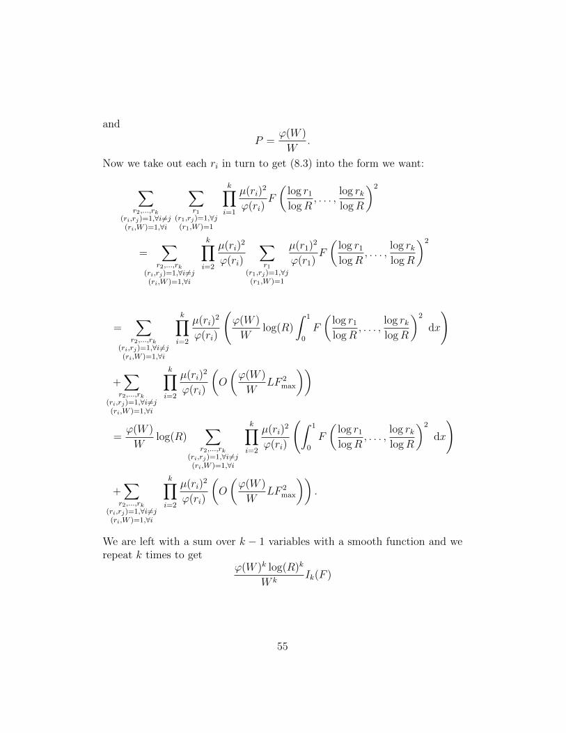
and

P =ϕ(W )

W.

Now we take out each ri in turn to get (8.3) into the form we want:

∑r2,...,rk

(ri,rj)=1,∀i 6=j(ri,W )=1,∀i

∑r1

(r1,rj)=1,∀j(r1,W )=1

k∏i=1

µ(ri)2

ϕ(ri)F

(log r1logR

, . . . ,log rklogR

)2

=∑

r2,...,rk(ri,rj)=1,∀i 6=j(ri,W )=1,∀i

k∏i=2

µ(ri)2

ϕ(ri)

∑r1

(r1,rj)=1,∀j(r1,W )=1

µ(r1)2

ϕ(r1)F

(log r1logR

, . . . ,log rklogR

)2

=∑

r2,...,rk(ri,rj)=1,∀i 6=j(ri,W )=1,∀i

k∏i=2

µ(ri)2

ϕ(ri)

(ϕ(W )

Wlog(R)

ˆ 1

0

F

(log r1logR

, . . . ,log rklogR

)2

dx

)

+∑

r2,...,rk(ri,rj)=1,∀i 6=j(ri,W )=1,∀i

k∏i=2

µ(ri)2

ϕ(ri)

(O

(ϕ(W )

WLF 2

max

))

=ϕ(W )

Wlog(R)

∑r2,...,rk

(ri,rj)=1,∀i 6=j(ri,W )=1,∀i

k∏i=2

µ(ri)2

ϕ(ri)

(ˆ 1

0

F

(log r1logR

, . . . ,log rklogR

)2

dx

)

+∑

r2,...,rk(ri,rj)=1,∀i 6=j(ri,W )=1,∀i

k∏i=2

µ(ri)2

ϕ(ri)

(O

(ϕ(W )

WLF 2

max

)).

We are left with a sum over k − 1 variables with a smooth function and werepeat k times to get

ϕ(W )k log(R)k

W kIk(F )

55

as our main term and we have error term

∑r1,...,rk−1

(ri,rj)=1,∀i 6=j(ri,W )=1,∀i

k∏i=2

µ(ri)2

ϕ(ri)

(O

(ϕ(W )

WLF 2

max

))

�∑

r1,...,rk−1

(ri,W )=1,∀i

k∏i=2

µ(ri)2

ϕ(ri)

(O

(ϕ(W )

WLF 2

max

))

=ϕ(W )k−1

W k−1(logR)k−1

(O

(ϕ(W )

WLF 2

max

))

= O

(F 2maxϕ(W )k(logD0)(logR)k−1

W k

).

Note that the error for every subsequent iteration will be smaller, so this isthe only one we need to worry about.

Substituting in, we get

S1 =N

W

ϕ(W )k log(R)k

W kIk(F ) +O

(F 2maxϕ(W )kN(logD0)(logR)k−1

W k+1

)(8.5)

+O

(F 2maxϕ(W )kN(logR)k

W k+1D0

).

Thenlog(R)

D0

≥ log(D0)

gives the result

S1 =N

W

ϕ(W )k log(R)k

W kIk(F ) +O

(F 2maxϕ(W )kN(logR)k

W k+1D0

).

Now we move on to the corresponding result for S2 and, as in Section 6,we will skip over the parts that are analogous to the S1 case.

56

Lemma 8.3. For yr, F , Fmax as in the previous lemma, we have

S(m)2 =

ϕ(W )kN(logR)k+1

W k+1 logNJ(m)k (F ) +O

(F 2maxϕ(W )kN(logR)k

W k+1D0

)with

J(m)k (F ) : =

ˆ 1

0

· · ·ˆ 1

0

(ˆ 1

0

F (t1, . . . , tk) dtm

)2

dt1 . . . dtm−1dtm+1 . . . dtk.

Proof. From Section 7, whenever we have

y(m)r1,...,rk

=∑am

yr1,...,rm−1,am,rm+1,...,rk

ϕ(am)+O

(ymaxϕ(W ) logR

WD0

),

whenever rm = 1 and r =∏k

i=1 ri satisfies both (r,W ) = 1 and µ(r) 6= 0 and

that y(m)r1,...,rk = 0 otherwise. We substitute for F in terms of yr, calling

Fr = F

(log r1logR

, . . . ,log rm−1

logR,log amlogR

,log rm+1

logR, . . . ,

log rklogR

)(8.6)

to get

y(m)r1,...,rk

=∑am

µ(am)2

ϕ(am)Fr +O

(ymaxϕ(W ) logR

WD0

). (8.7)

Similar to before, we apply Lemma 6.2, here taking

γ(p) =

{1, p - Wr

0 p | Wr,

to which Lemma 6.2 applies with L = log logN . However, this time we’renot going to apply it k times, instead we apply it just once.

Again, to simplify the equation, let

F (m)r :=

ˆ 1

0

F

(log r1logR

, . . . ,log rm−1

logR, tm,

log rm+1

logR, . . . ,

log rklogR

)dtm, (8.8)

Then we get

y(m)r1,...,rk

=ϕ(W ) log(R)

W

(k∏

i=1

ϕ(ri)

ri

)F (m)r +O

(ymaxϕ(W ) logR

WD0

).

57

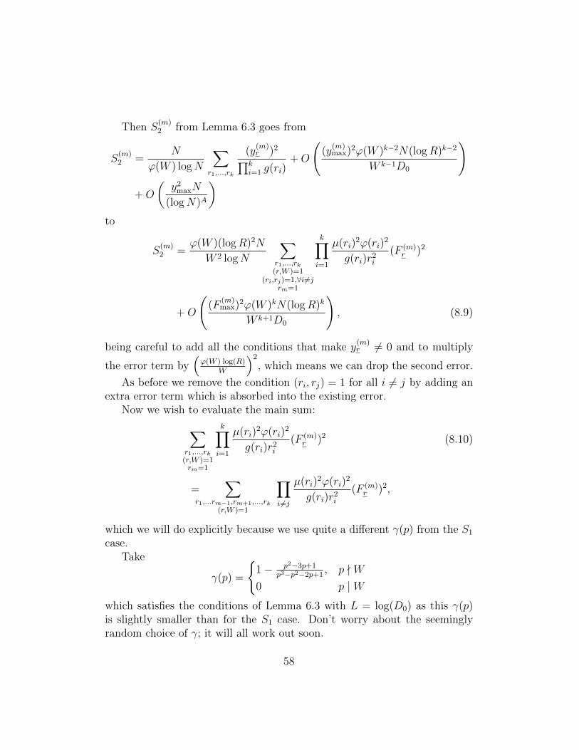
Then S(m)2 from Lemma 6.3 goes from

S(m)2 =

N

ϕ(W ) logN

∑r1,...,rk

(y(m)r )2∏k

i=1 g(ri)+O

((y

(m)max)2ϕ(W )k−2N(logR)k−2

W k−1D0

)

+O

(y2maxN

(logN)A

)to

S(m)2 =

ϕ(W )(logR)2N

W 2 logN

∑r1,...,rk(r,W )=1

(ri,rj)=1,∀i 6=jrm=1

k∏i=1

µ(ri)2ϕ(ri)

2

g(ri)r2i(F (m)

r )2

+O

((F

(m)max)2ϕ(W )kN(logR)k

W k+1D0

), (8.9)

being careful to add all the conditions that make y(m)r 6= 0 and to multiply

the error term by(

ϕ(W ) log(R)W

)2, which means we can drop the second error.

As before we remove the condition (ri, rj) = 1 for all i 6= j by adding anextra error term which is absorbed into the existing error.

Now we wish to evaluate the main sum:∑r1,...,rk(r,W )=1rm=1

k∏i=1

µ(ri)2ϕ(ri)

2

g(ri)r2i(F (m)

r )2 (8.10)

=∑

r1,...rm−1,rm+1,...,rk(r,W )=1

∏i 6=j

µ(ri)2ϕ(ri)

2

g(ri)r2i(F (m)

r )2,

which we will do explicitly because we use quite a different γ(p) from the S1

case.Take

γ(p) =

{1− p2−3p+1

p3−p2−2p+1, p - W

0 p | W

which satisfies the conditions of Lemma 6.3 with L = log(D0) as this γ(p)is slightly smaller than for the S1 case. Don’t worry about the seeminglyrandom choice of γ; it will all work out soon.

58

We have, whenever γ(p) is non-zero,

η(p) =

(1− p2 − 3p+ 1

p3 − p2 − 2p+ 1

)(p− p3 − 3p2 + p

p3 − p2 − 2p+ 1

)−1

and the auxiliary function

P =∏

p primep -W

(1− 1

p+

1

p

p2 − 3p+ 1

p3 − p2 − 2p+ 1

)−1(1− 1

p

) ∏p primep|W

(1− 1

p

).

Here’s where the strange choice of γ(p) comes to fruition; we chose it thisway so that η(p) is the coefficient of µ(d)2F (d), i.e.

η(p) =

(1− p2 − 3p+ 1

p3 − p2 − 2p+ 1

)(p− p3 − 3p2 + p

p3 − p2 − 2p+ 1

)−1

=(p3 − 2p2 + p

) (p4 − 2p3

)−1

=(p− 1)2

(p− 2)p2

=ϕ(p)2

g(p)p2,

which tells us that we can apply the lemma in exactly the same way we didfor S1, pulling out each ri term (i 6= m) in turn.

We note that p2− 3p+1 is positive for all p ≥ 2, so our P is even smallerthan for S1 and we can use the same bound. Then with (k − 1) different rivariables to work over (not k as previously), we get∑

r1,...rm−1,rm+1,...,rk(r,W )=1

∏i 6=j

µ(ri)2ϕ(ri)

2

g(ri)r2i(F (m)

r )2

=ϕ(W )k−1 log(R)k−1

W k−1J(m)k (F )

and

S(m)2 =

ϕ(W )kN log(R)k+1

W k+1 logNJ(m)k (F ) +O

((F

(m)max)2ϕ(W )kN(logR)k

W k+1D0

),

as required.

59

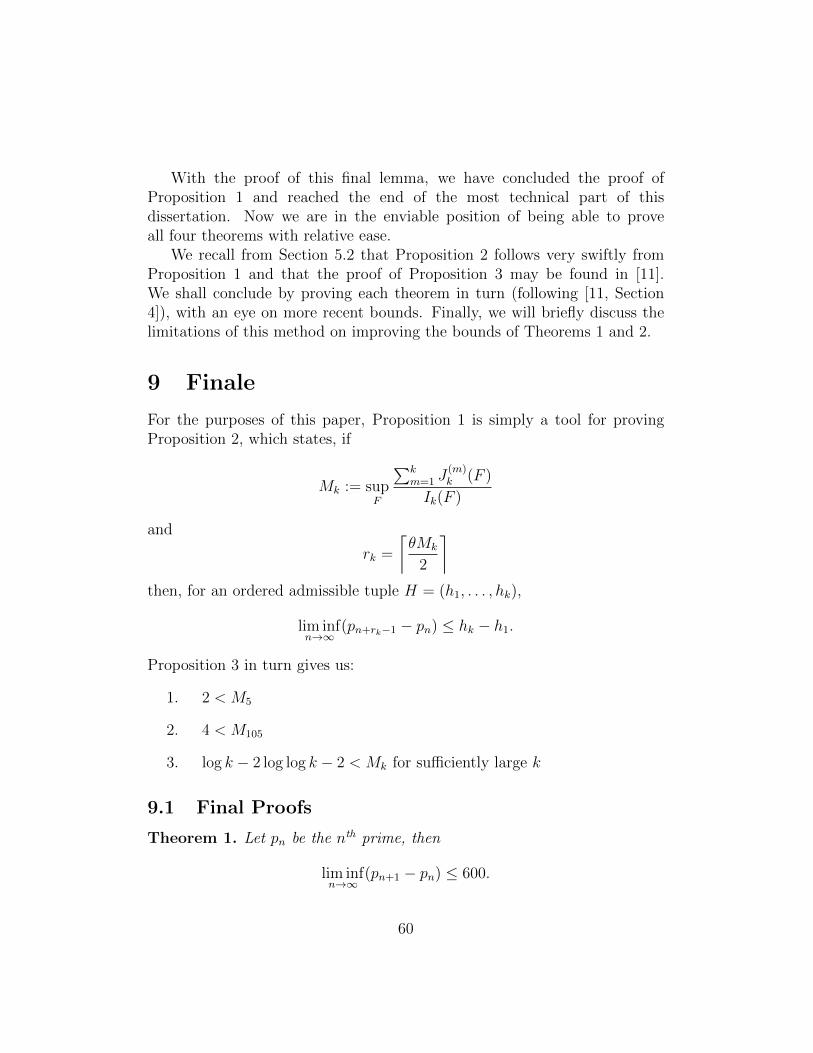
With the proof of this final lemma, we have concluded the proof ofProposition 1 and reached the end of the most technical part of thisdissertation. Now we are in the enviable position of being able to proveall four theorems with relative ease.

We recall from Section 5.2 that Proposition 2 follows very swiftly fromProposition 1 and that the proof of Proposition 3 may be found in [11].We shall conclude by proving each theorem in turn (following [11, Section4]), with an eye on more recent bounds. Finally, we will briefly discuss thelimitations of this method on improving the bounds of Theorems 1 and 2.

9 Finale

For the purposes of this paper, Proposition 1 is simply a tool for provingProposition 2, which states, if

Mk := supF

∑km=1 J

(m)k (F )

Ik(F )

and

rk =

⌈θMk

2

⌉then, for an ordered admissible tuple H = (h1, . . . , hk),

lim infn→∞

(pn+rk−1 − pn) ≤ hk − h1.

Proposition 3 in turn gives us:

1. 2 < M5

2. 4 < M105

3. log k − 2 log log k − 2 < Mk for sufficiently large k

9.1 Final Proofs

Theorem 1. Let pn be the nth prime, then

lim infn→∞

(pn+1 − pn) ≤ 600.

60

Proof. By Proposition 3, M105 < 4. By Bombieri - Vinogradov, we can takeθ = 1

2− ε for ε > 0.

Then we find, in Proposition 2,

rk >12× 4

2= 1

sork = 2

and then we havelim infn→∞

(pn+1 − pn) ≤ h105 − h1.

This means we need to find an admissible tuple of length 105. The smallestpossible such tuple was found by Clark-Jarvis and has length 600,3 whichgives our result.

Using work from [15] along with Maynard’s results, the Polymath projecthas concluded with this bound reduced to 246 [16].

Theorem 2 is the corresponding result for θ = 1− ε:

Theorem 2. Assuming Elliott - Halberstam, we have:

lim infn→∞

pn+1 − pn ≤ 12.

Proof. This is identical to the previous proof except we may now use M5 < 2to give rk = 2.

The smallest admissible tuple of length 5 is (0, 4, 6, 10, 12), proving thissecond theorem.

Polymath gives that this can in fact be taken as low as 6.Finally, we have the general case, looking at m being large (for 2 ≤ m ≤ 5

the reader may like to look at [16, Theorem 1.4]).

Theorem 3. Let pn be the nth prime number, m ∈ N, then we have

lim infn→∞

(pn+m − pn) � m3e4m.

3For any readers who enjoy looking at long lists of prime k-tuples, this one and manyothers can be found at math.mit.edu/˜primegaps/ which is run by Andrew Sutherland

61

Proof. We’re looking for a similar proof to the two previous theorems, exceptnow we have

rk >

( 12− ε

2

)(log k − 2 log log k − 2)

which we want to be greater than m. Taking ε to be 1kgives us

k ≥ Cm2e4m

for some constant C which is independent of k and m. Then to get thisminimal we must take

k =⌈Cm2e4m

⌉and find a corresponding k-tuple. Recall that for admissibility we requireH = (h1, . . . , hk) to have hi all avoiding some residue class modulo eachprime less than k. This leads us towards one way of building an admissiblek-tuple for any k: we start at the first prime number after k and take thenext k− 1 prime numbers after that; then none of our hi ≡ 0 mod p, for anyp ≤ k and our H is admissible. Using this construction we obtain

H = (pπ(k)+1, . . . , pπ(k)+k),

which has diameter pπ(k)+k−pπ(k)+1 � k log k by the prime number theorem.Then

lim inf(pn+m − pn) � k log k

and substituting in our value for k, we get

lim inf(pn+m − pn) � Cm3e4m.

Again, Polymath8b gives us a slightly improved bound, this time ofCme2m.

The last theorem says that the prime k-tuples conjecture is true for apositive proportion of admissible k-tuples. Though we fully expect it to betrue for all admissible k-tuples, this partial result is a useful step in the rightdirection.

Theorem 4. Let A = {a1, a2, . . . , ar} be an admissible set of distinct integersand H = {h1, h2, . . . , hk} be a subset of A containing k < r elements. Then

62

for a positive proportion of such H, {n + hi}ki=1 are all prime for infinitelymany n.

Equivalently,

|{H ⊆ A : H satisfies the prime k-tuples conjecture}||{H ⊆ A}|

� 1.

As the statement of Theorem 4 is different from that given by Maynard,this proof is also quite different to the one he provides.

Proof. Given m, let k = dCm2e4me as above. First take r = k and let A ={a1, a2, . . . , ar} be an admissible set of distinct integers. Then by Theorem3, there exists a subset H = {h1, h2, ..., hm} of A such that all {n+ hi}mi=1

are prime infinitely often. Explicitly then, we have that at least 1 of the 2r

subsets of A satisfies the prime m-tuples conjecture. What we must show isthat this proportion stays positive as r grows.

Claim. For any r > k,A = {a1, a2, . . . , ar}, the proportion of subsets of Awhich satisfy the prime m-tuples conjecture is greater than or equal to

|{B ⊆ A : |B| = k}||{B ⊆ A}|

.

Proof. Let A1 = {a1, a2, . . . , ar+1} be admissible. Then for each hi in Hwe may take A1\{hi} to obtain m admissible sets, each comprised of rintegers, each possessing a different set Hi which satisfies the prime m-tuplesconjecture.

The claim then follows by induction on the size of A1.

To get the theorem we have to bound this fraction. Each part can beevaluated with basic counting arguments, which give

|{B ⊆ A : |B| = k}| =(

rk

),

where the right hand side is the binomial coefficient, and

|{B ⊆ A}| = 2r.

This means our proportion has become

r!

2rk!(r − k)!.

63

As r tends to infinity the r! and (r − m)! terms dominate, bringing ourproportion closer to 1 and giving the result

|{B ⊆ A : |B| = k}||{B ⊆ A}|

� 1.

This paper has been a demonstration of the power of sieve methods, butthere is a huge obstacle in the way of further progress (reducing the limitbelow lim infn→∞(pn+1 − pn) ≤ 6), known as the parity problem. The parityproblem was first described by Selberg himself in 1949 [17], and it basicallysays that sieves cannot distinguish between integers with an even or oddnumber of prime factors. In our case, that means they cannot distinguishbetween primes and ‘almost-primes’, numbers that are the products of twoprimes. This is perhaps best emphasised by Chen’s Theorem [1], which statesthat the Twin Prime Conjecture, and even the more general de Polignac’sconjecture, are true if we loosen the conditions to include almost-primes.What this means for us is that if, using sieve theory, we could get anybound that said lim infn→∞(pn+1 − pn) < 6, then we would also be able toprove certain completely contradictory statements. A more detailed versionof this, including a heuristic of the contradictory statements can be seenin [16, Section 8]. It suffices to say that any improvement, in particular anyproof of the Twin Prime Conjecture using sieve methods, will require a new,considerable breakthrough in sieve theory.

9.2 Acknowledgements

I would like to thank my supervisor Jennifer Balakrishnan for all her timeand effort in helping me put this dissertation together and James Maynardfor a very useful maths lesson.

64

References

[1] J. R. Chen. On the representation of a large even integer as the sumof a prime and the product of at most two primes. KeXue Tong Bao,17:385 – 386, 1966. In Chinese.

[2] P. Elliott and H. Halberstam. A conjecture in prime number theory.Symposia Mathematica, 4:59 – 72, 1970.

[3] J. Friedlander and A. Granville. Limitations to the equi-distributions ofprimes i. Annals of Mathematics, 129:363 – 382, 1989.

[4] D. Goldston, S.W. Graham, J. Pintz, and C. Yıldırım. Smallgaps between products of two primes. Proceedings of the LondonMathematical Society, 98:741 – 774, 2009.

[5] D. Goldston, J. Pintz, and C. Yıldırım. Primes in tuples I. Annals ofMathematics, 170:819 – 862, 2009.

[6] T. Gowers. Is massively collaborative mathematicspossible? https://gowers.wordpress.com/2009/01/27/

is-massively-collaborative-mathematics-possible/, 2009.Last Accessed 20/03/2015.

[7] A. Granville. Bounded gaps between primes. http://www.

dms.umontreal.ca/~andrew/CurrentEventsArticle.pdf, 2014. Lastaccessed 20/03/2015.

[8] D. R. Heath-Brown. Almost-prime k-tuples. Mathematika, 44:245 – 266,1997.

[9] E. Landau. Handbuch der Lehre von der Verteilung der Primzahlen,volume 1. Leipzig B.G. Teubner, 1909.

[10] A. Legendre. Essai sur la theie des nombres. 1798.

[11] J. Maynard. Small gaps between primes. Annals of Mathematics,181:383 – 413, 2015.

[12] H. L. Montgomery and R. C. Vaughan. Multiplicative Number TheoryI: Classical Theory. Cambridge University Press, 2006.

65

[13] S. Nazardonyavi. Some history about twin prime conjecture. http:

//arxiv.org/abs/1205.0774v1, 2012. Last Accessed 20/03/2015.

[14] A. de Polignac. Six propositions arithmologiques deduites du cribled’Eratosthene. Nouvelles annales de mathematiques 1re serie, 8:423 –429, 1849.

[15] D. H. J. Polymath. New equidistribution estimates of Zhang type.Algebra and Number Theory, 8:2067 – 2199, 2014.

[16] D. H. J. Polymath. Variants of the Selberg sieve, and bounded intervalscontaining many primes. Research in the Mathematical Sciences, 1:12,2014.

[17] A. Selberg. On elementary methods in prime number theory and theirlimitations. Den 11te Scandinaviske Matematikerkongress, Trondheim,pages 13 – 22, 1949.

[18] A. Selberg. Lectures on Sieves. Collected Works, vol. 2. Springer-Verlag,1991.

[19] T. Tao. Polymath8. https://terrytao.wordpress.com/tag/

polymath8/, 2014. Last Accessed 20/03/2015.

[20] T. S. Trudgian. A poor man’s improvement on zhang’s result: there areinfinitely many prime gaps less than 60 million. http://arxiv.org/

abs/1305.6369/, 2013. Last Accessed 20/03/2015.

[21] A. I. Vinogradov. On the density hypothesis for Dirichlet L-functions.Akademiia nauk SSSR Ser. Math., 29:903 – 934, 1965.

[22] A. Wilkinson. The Pursuit of Beauty. http://www.newyorker.

com/magazine/2015/02/02/pursuit-beauty, 2015. Last Accessed20/03/2015.

[23] Y. Zhang. Bounded gaps between primes. Annals of Mathematics,179:1121 – 1174, 2013.

66