Boundary Layers in the Mantle;

a Tomographer’s View

Adam M. Dziewoński

VLAB Workshop, August 10, 2007

In cooperation with:Gőran EkstrőmYu Jeffrey GuBogdan Kustowski

ScS – S elephant;the need for global 3-D

thinking

Power spectra of three recent models

Harvard Caltech Berkeley

Surface

T.Z.

C.M.B

Power spectra of the three models;

a closer look Harvard Caltech Berkeley

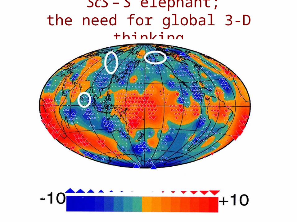
It cannot be that simple

Grand et al., 1997

Diverse data sets is what

made the progress possible

Data – the critical element

Three types of data are needed: 1. Fundamental mode surface waves to resolve the near surface structure;

2. Overtone data to resolve structure in the transition zone and

3. Travel time data to resolve the lower mantle structure.

Only three research groups (Berkeley, Caltech/Oxford and Harvard) use this, or equivalent, combination of data

Fundamental mode surface waves

Rayleigh 75 seconds

Love35 seconds

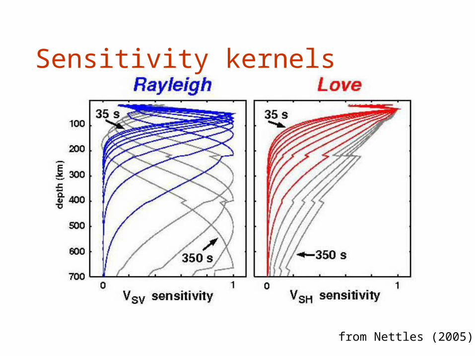
Sensitivity kernels

from Nettles (2005)

Long-period body wave waveforms

from Gu et al. (2001)

Mantle wave waveforms

from Gu et al. (2001)

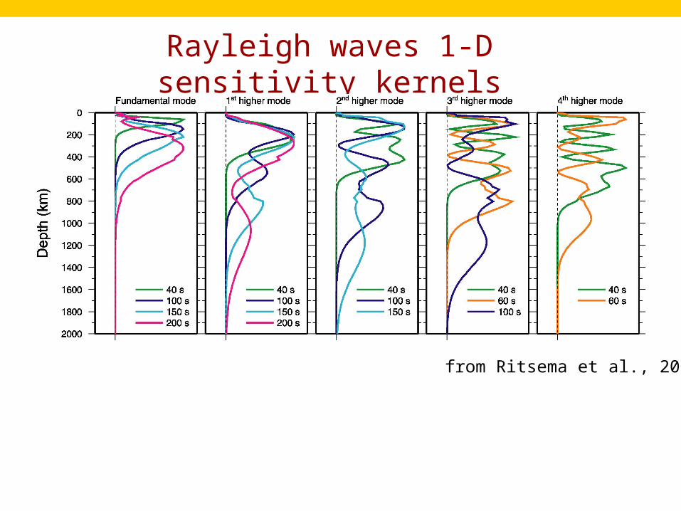
Rayleigh waves 1-D sensitivity kernels

from Ritsema et al., 2004

Body wave travel times

CMB 650 km Moho

Depth resolution of different data subsets

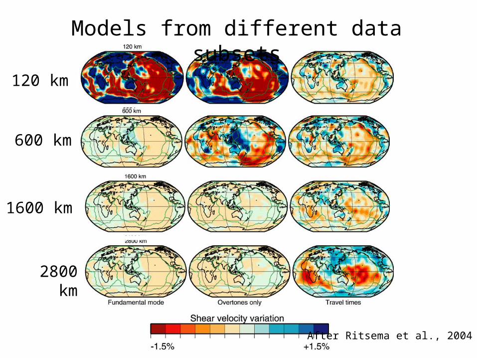
Models from different data subsets

120 km

600 km

1600 km

2800 km

After Ritsema et al., 2004

Surface Boundary Layer

Velocity

lowattenuation

highattenuation

Attenuation

Recent velocity modelsare very well correlatedin the top 200 km, or so, of the mantle

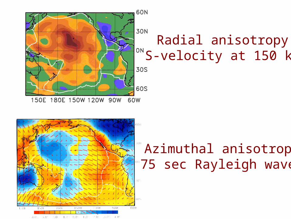
Radial anisotropyS-velocity at 150 km

Azimuthal anisotropy75 sec Rayleigh waves

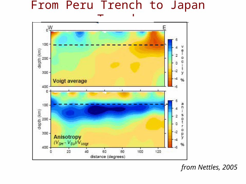
From Peru Trench to Japan Trench

from Nettles, 2005

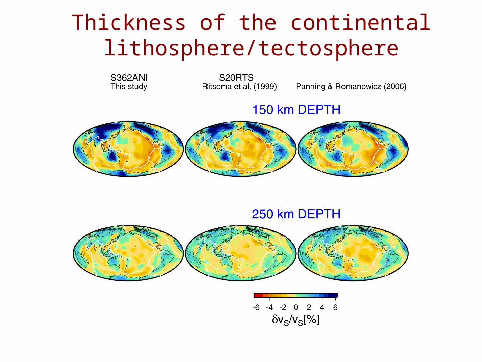
Thickness of the continental lithosphere/tectosphere

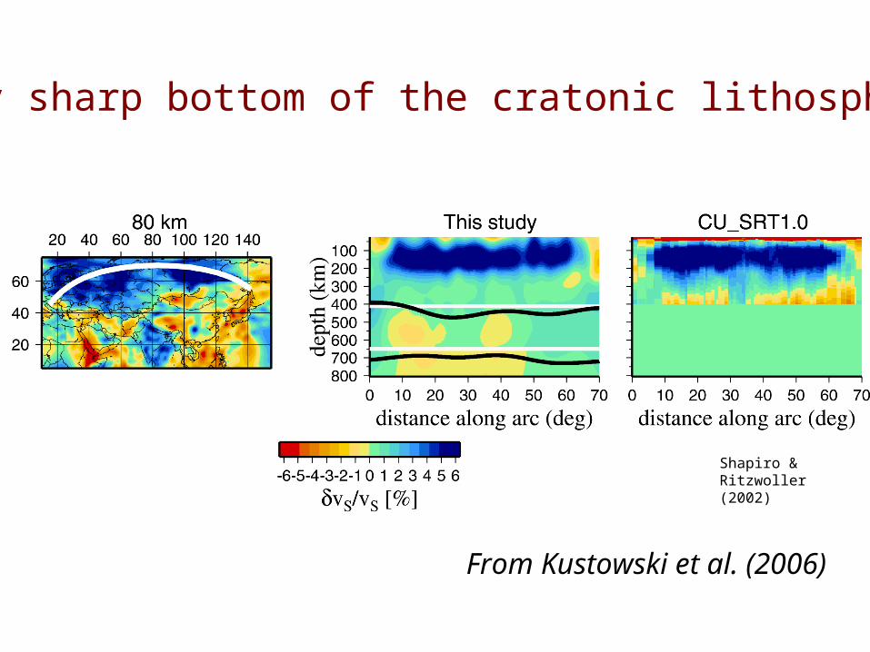
Shapiro & Ritzwoller (2002)

Very sharp bottom of the cratonic lithosphere

From Kustowski et al. (2006)

Questions:• What processes cause radial anisotropy in a 100 Ma old oceanic lithosphere at a depth of 150 km?

• Why are the isotropic velocity anomalies correlated with the age of the oceanic plate down to a depth of 200 km, even though plate cooling models prefer 100 km thickness?

• What is the thickness of the continental lithosphere

Transition Zone

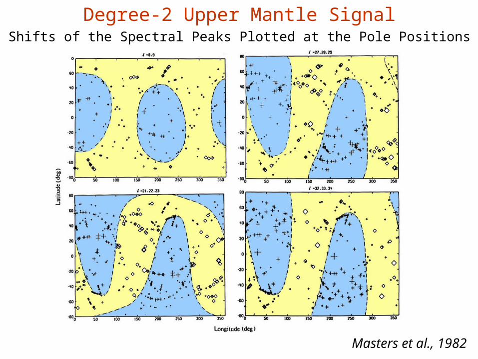
Degree-2 Upper Mantle SignalShifts of the Spectral Peaks Plotted at the Pole Positions

Masters et al., 1982

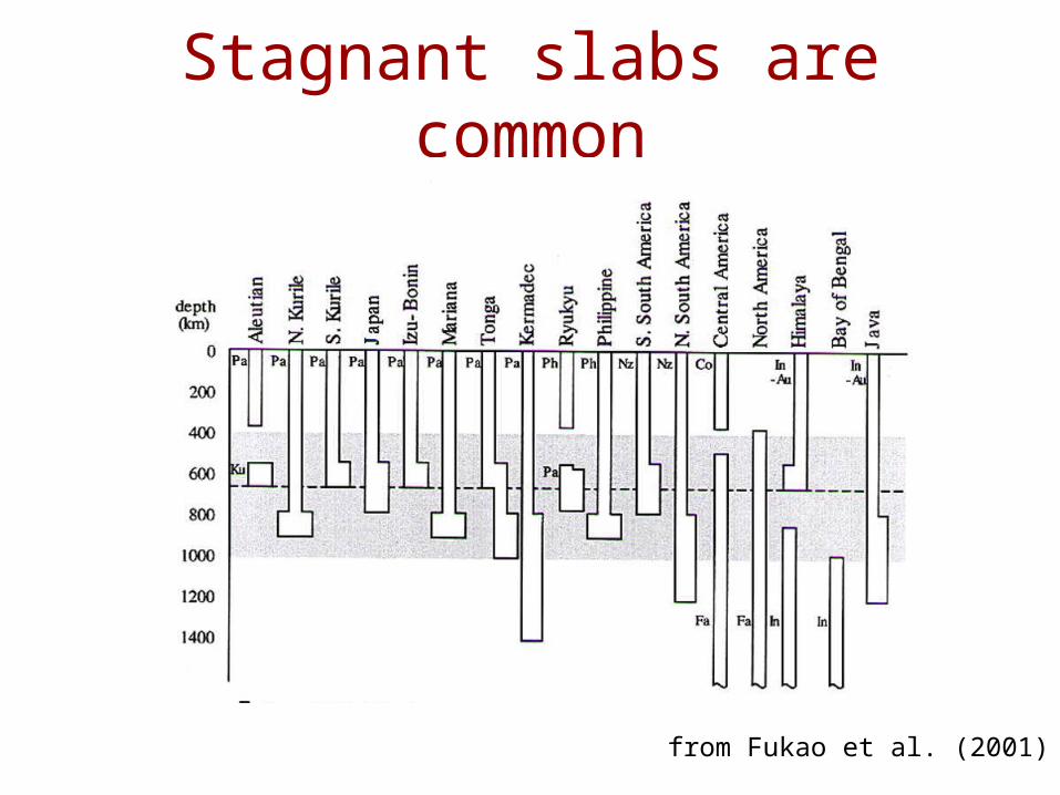
Stagnant slabs are common

from Fukao et al. (2001)

Patterns of velocity anomalies above and below the 670 km discontinuity are not similar

From Gu et al. (2001)

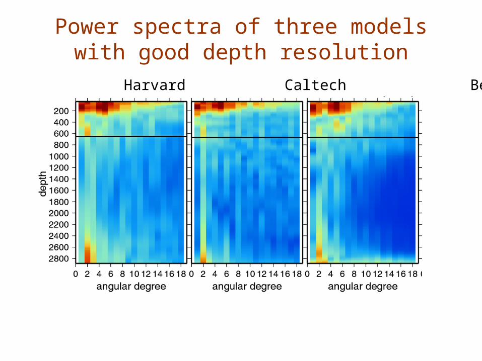
Power spectra of three modelswith good depth resolution

Harvard Caltech Berkeley

600 km depth

800 km depth

Harvard Caltech Berkeley

Additionalevidence

Change in the stress pattern near the 650 km discontinuity

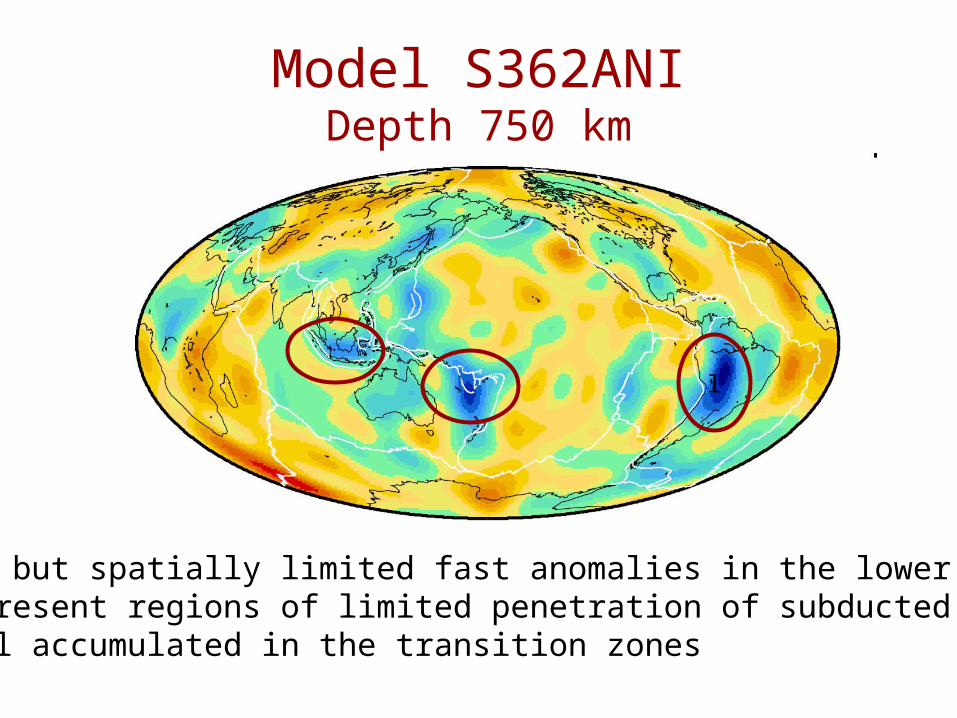
Model S362ANIDepth 750 km

Strong, but spatially limited fast anomalies in the lower mantle may represent regions of limited penetration of subducted material accumulated in the transition zones

l

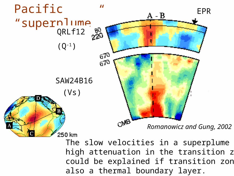
Pacific “superplume”

Romanowicz and Gung, 2002

QRLf12

(Q-1)

SAW24B16

(Vs)

The slow velocities in a superplume andhigh attenuation in the transition zonecould be explained if transition zone isalso a thermal boundary layer.

EPR

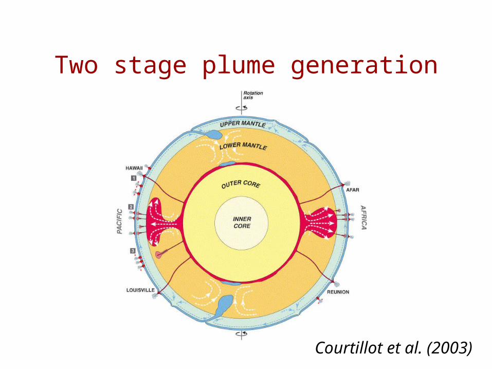
Two stage plume generation

Courtillot et al. (2003)

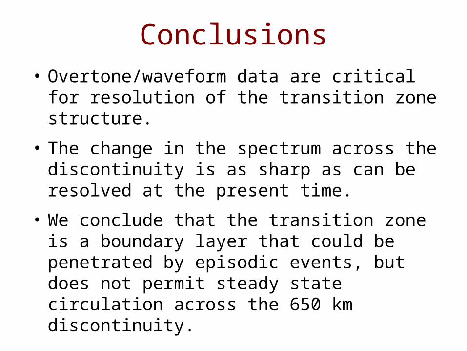
Conclusions• Overtone/waveform data are critical for resolution of the transition zone structure.

• The change in the spectrum across the discontinuity is as sharp as can be resolved at the present time.

• We conclude that the transition zone is a boundary layer that could be penetrated by episodic events, but does not permit steady state circulation across the 650 km discontinuity.

Lowermost Mantle

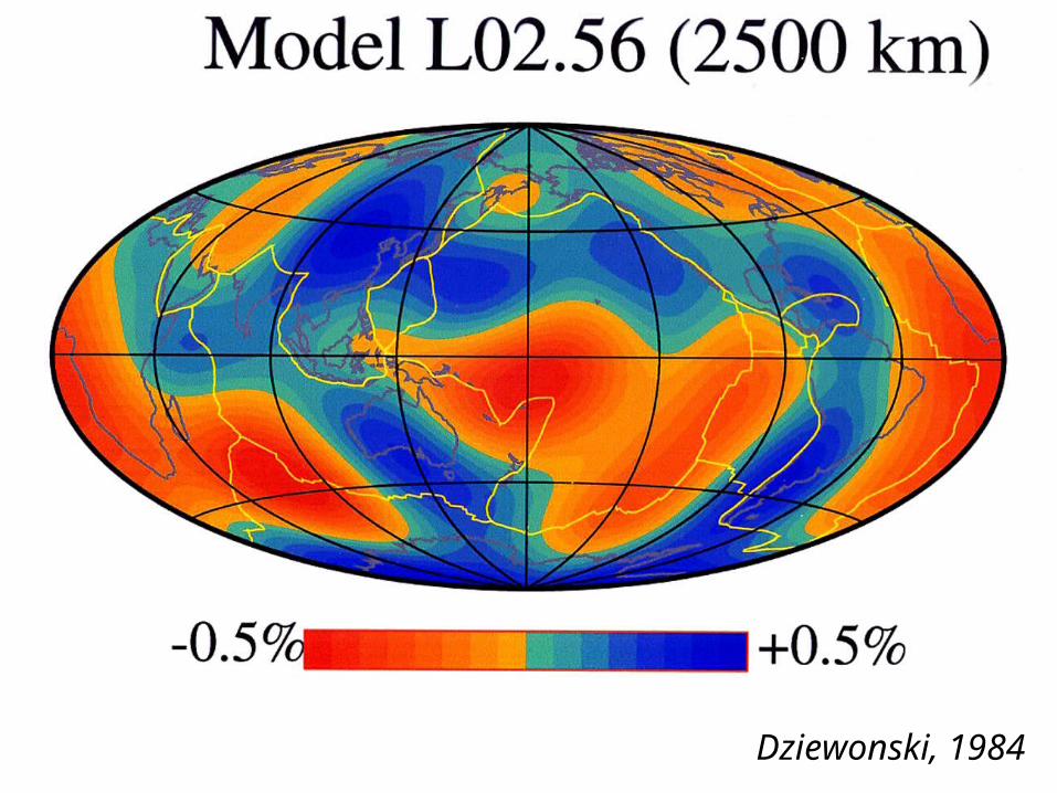
Dziewonski, 1984

Equatorial Cross-section

Dziewonski (1984) and Woodhouse and Dziewonski (1984)

Megaplumes span whole lower

mantle

3-D view of +0.5% and -0.5% isosurfaceof S-velocity modelof Masters et al. (2000). The uppersurface is truncated at 800 km depthand lower – at CMB

Usually, models of the shear and compressional velocity are obtained independently. However, P-velocity depends both on shear modulus and bulk modulus. To isolate this interdependence, Su and Dziewonski (1997) formulated the inverse problem for a joint data set and derived 3-D perturbations of bulk sound velocity and shear velocity

Model of shear and bulk sound velocities

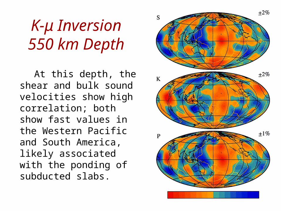
K-μ Inversion550 km Depth

At this depth, the shear and bulk sound velocities show high correlation; both show fast values in the Western Pacific and South America, likely associated with the ponding of subducted slabs.

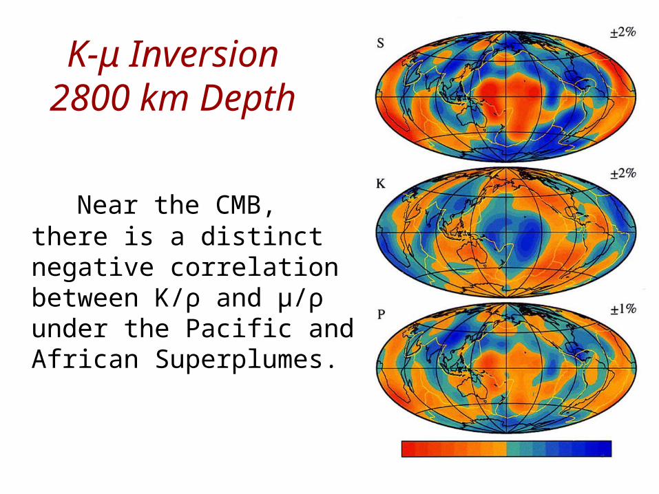
K-μ Inversion2800 km Depth

Near the CMB, there is a distinct negative correlation between K/ρ and μ/ρ under the Pacific and African Superplumes.

Bulk Sound and Shear Velocity Anomalies

Correlation between the bulk sound and shear velocity anomalies changes from +0.7 in the transition zone to –0.8 in the lowermost mantle. From Su and Dziewonski, 1997.

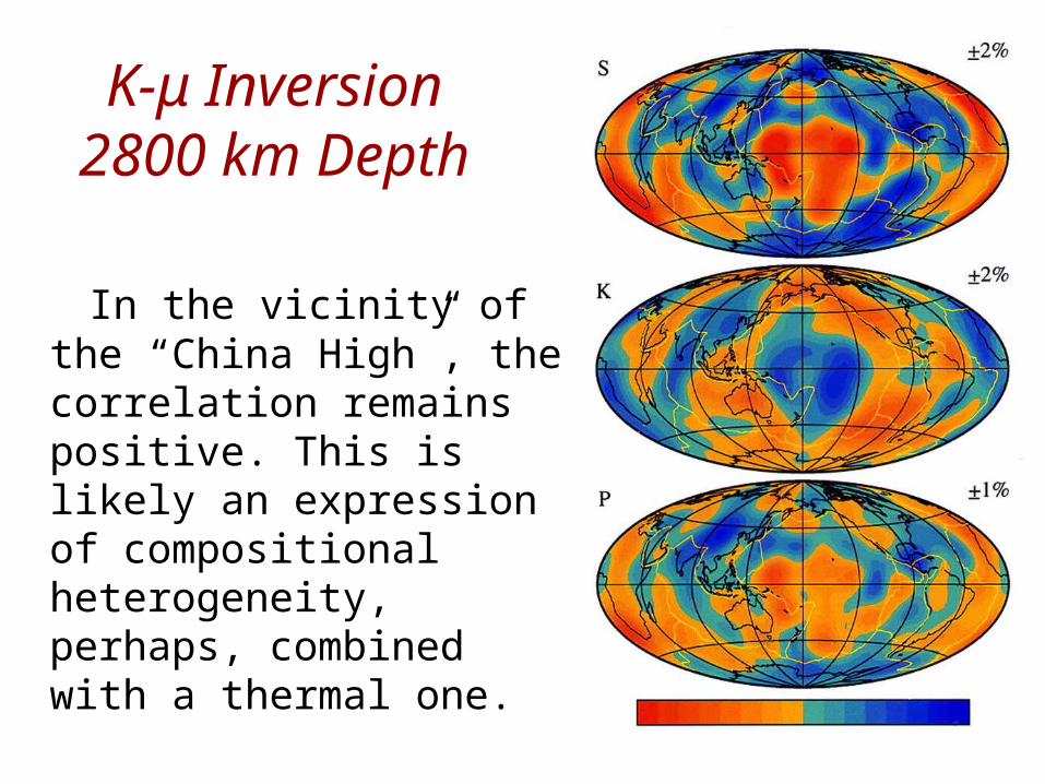
K-μ Inversion2800 km Depth

In the vicinity of the “China High”, the correlation remains positive. This is likely an expression of compositional heterogeneity, perhaps, combined with a thermal one.

Questions:

• How have the super-plumes formed?• What part of the anomalies is caused by compositional rather than thermal variations?

• Why do the super-plumes continue across the D” without an apparent change in the amplitude of the anomaly?