Boundary Element Method to the potential flow around ...

Some numerical aspects of the application of the

Boundary Element Method to the potential flow

around propellers

J.A.C. Falcao de Campos, R.S. Duarte, J.L.M. Fernandas

MARETEC/DEM, Department of Mechanical Engineering,

Institute Superior Tecnico, 1096 Lisboa Codex, Portugal

Abstract

A boundary element method (BEM) is applied to the computation of the steady,incompressible flow around propellers. The method is based on Morino's^formulation for the disturbance potential. The method uses constant dipole andsource singularity distributions on flat or hyperboloidal panels. The paperdiscusses the basic choices made to evaluate the matrix of influencecoefficients and the use of direct and iterative solvers in the solution of thesystem of equations. It is shown that the use of hyperboloidal elementsimproves the convergence of the numerical solution.

1 Introduction

In recent years the boundary element method (BEM) has become in the shiphydrodynamics community an increasingly important tool to compute thepotential flow around marine propulsors. One of the first applications topropellers based on a velocity formulation was published by Hess andValarezo* However, the most common approach is based on Green's identityformula for the disturbance potential as originally proposed by Morino^. For thespecific propeller application a number of numerical implementations havebeen developed along these lines, Kerwin et al. , Lee\ Hoshino^ for steadyflow and Kinnas et al , Hsin\ Koyama® and Hoshino^ for unsteady flow.Recently, the various boundary element methods for propellers (surface panelmethods, as they are called in the hydrodynamic literature) have been evaluatedthrough comparative calculations and comparison with experimental data fortwo sample propellers in a workshop organized by the 20^ ITTC PropulsorCommittee, (see Koyama ). The results can be considered to represent the

Transactions on Modelling and Simulation vol 12, © 1996 WIT Press, www.witpress.com, ISSN 1743-355X

528 Boundary Elements

present state-of-the-art of the application of the boundary element method tomarine propellers in steady flow.

Most of the methods previously mentioned are based on the sameformulation and similar numerical implementations, but the accuracy of theresults in specific cases may vary considerably, as clearly shown by the scatterof the results shown in the comparative calculations (see Koyama ). Theoverall accuracy of the results depends critically on the modeling of generaland detailed features of the flow field, such as the modeling of the wakes of thepropeller blades and the flow at the trailing edge, the adequacy of the surfacegrids and of a number of options concerning the numerical approximations.Also the computational efficiency and robustness of the methods are stronglydependent on many of the numerical procedures adopted in a particularimplementation.

. This paper describes the current status of a boundary element method for thecomputation of the steady incompressible flow around a propeller anddiscusses some of the basic options that were made for this specific application.These concern the type of element, the calculation of the matrix influencecoefficients and the use of direct and iterative solvers for the solution of theresulting linear system of equations. The formulation is briefly reviewed insection 2 and the numerical method is described in section 3. In section 4results are presented and discussed for one of the sample propellers employedin the comparative calculations of Koyama^.

2 Potential flow problem

Consider a right-hand propeller of radius Rp rotating with constant angular

speed Q and advancing with constant velocity U in an infinite ideal andincompressible fluid. The propeller has K blades symmetrically arrangedaround an axisymmetric hub. A cartesian and a cylindrical coordinate systemsfixed with the propeller blades are used to describe the propeller geometry andthe flow field. Figure 1 shows the propeller and coordinate system conventions.

Figure 1: Propeller coordinate systems

In a reference frame fixed to the propeller blades the flow is steady and the

flow velocity V(x,y,z) may be described by the perturbation potential (j)(x,y,z)

according to


Boundary Elements 529

where

&L=C/r + OrZe (2)

is the undisturbed velocity. The potential flow problem is governed by theLaplace equation

V2# = 0, (3)

with boundary conditions

d<b-^ = n-V(f) = -n-U^ on SB and S^ (4)an

V(f) — > 0 if x — > -oo or r — > <*> , (5)

and the Kutta condition

V0 < oo (7)

at the blade trailing edge. In equations (4) and (6) n is the unit normal directedoutwards from the body, SQ, S^ and S\y the blades', the hub and the wakes'

surfaces, respectively, p the pressure and the subscripts + and - denote the two

sides of the blade wake corresponding to the blade suction and pressure sidesrespectively.

The application of the third Green's identity for the potential of a pointP(x,y,z) on the surfaces j>#, and S// , with the use of the boundary condition

(4) (Morino\ Kerwin et al? , Hoshino^) gives

where A0( 2') represents the potential jump on the wake. The integrals on S#

and S// in equation (8) should be interpreted as Cauchy principal values when



P —» Q. Equation (8) is a Fredholm integral equation of the second kind in the

potential values 0(0 on the surfaces S# e S//. The Kutta condition (7)

provides the additional relation to determine the potential jump A0(Q') on the

wake.The perturbation velocity tangent to the surface can be obtained by

differentiation on the surface of the potential distribution 0(<2) • The pressure

on the surface can be obtained from the Bernoulli equation in the form

_ «, _" "

. 2Vt

(9)

where p^ is the undisturbed pressure, p the fluid density, U^ = U^ and V,

the total velocity tangent to the surface.

3 Numerical method

3.1 Discretized system

For the numerical solution of the integral equation (8) the surfaces S$, S//

and S\y are discretized by quadrilateral elements. Two types of panels have

been used: hyperboloidal panels (Morino , Hoshino^) with straight edgesjoining the four quadrilateral vertices on the surface and flat panels (Kerwin etal?, Lee*) with vertices defined by the projections of the surface points on thetangent plane through the element centroid. On each element the singularitydistributions (dipole and sources) are assumed constant. A local error analysis(Romate**) reveals that for second order truncation error in the size of theelement, linear dipole and constant source distributions need to be used withflat elements on smooth surfaces and with quadratic elements on non-smoothsurfaces. In our case the formulation is not consistent but offers the advantageof considerable simplicity. As claimed by various authors (Kinnas et al?,Hsin ) the use of hyperboloidal panels in highly twisted propeller geometriesmay improve considerably the accuracy of the method.

The discretized system writes

N ^R N%( ._D .)0y- IW^A^= lB,y(a.[L)y, ;' = 1,2,...,7V, (10)7 = 1 7 = 1 7 = 1

where N is the number elements on the surface S# u S^, NR the number of

dipole strips on the blade wake, 8^ is the Kronecker delta and Dy , W^ and

BIJ are influence coefficients given by



KI

/r ^ ,%• = S I

6 = 1/-I

ifl^- R(Pi,(

-Lj/^ L_2?r/ a g /?( ,g)

-dS

dS

KI -d5

(11)

(12)

(13)

In equations (11) to (13) S^ denotes the jth element on the kth propeller

blade or hub sector and S^ the / th element on the j th wake strip from the

k th propeller blade. N^ is the streamwise number of elements on each wakestrip.

The calculation of the influence coefficients for flat elements can be madeanalytically using the formulation published by Newman^. Alternativeanalytical formulas valid for hyperboloidal panels were given by Morino^.These formulas are only exact for dipole coefficients, the source coefficientsbeing only exact for a flat element. For a twisted element the source coefficientformulas are a good approximation for small distances from the elementcentroid but their accuracy rapidly deteriorates with the distance from theelement. This is not a severe disadvantage since numerical integration is to bepreferred at increasing distances from the element from the point of view ofcomputational efficiency.

PRECISION

Iff*Iff*W*Iff*ia*la*

FUNCTION

SourceDipoleSourceDipoleSourceDipole

ANALYTIC

d<7.2d<2.2d<2.7d<J.Pd<J.7d<2.&

BURNSIDE

2.<3<d<7.

G.-L.2X2

7.2<d<632.2<d<742.7<d<2019<dJ.7<d7<d

G.-L.1X165<d74<d20<d

Table 1 Precision (relative error) achieved by various formulations for thecomputation of influence coefficients of a flat element as a function of therelative distance d to the element centroid (distance normalized by the elementlargest diagonal).



As an illustration, Table 1 presents for a flat element and different precisionrequired in the computation of the influence coefficients, the most efficientchoice as a function of the distance to the element. The following formulationswere investigated: analytical formulas (Morino ), integration with Gauss-Legendre, Burnside and Tyler rules and multipole expansions (3 terms).

3.2 Implementation of the Kutta condition

Morino^ introduced a Kutta condition requiring the potential jump in the waketo be equal to the difference between the potentials of the last elements at thetrailing edge

A^=0;-0/, y = 1,2,. ..,#*. (14)

This condition combined with rigid wake models does not ensure theequality of pressure on both sides of the blade at the trailing edge as requiredphysically (Kerwin et a/.\ Lee"*). The equal pressure condition at the trailingedge elements can be enforced by adjusting the dipole strength in the wake.The condition writes

(ACp),. =(C;),.-(C-),=0, ,' = l,2,...,#a. (15)

Due to the non-linear character of the pressure the Newton-Raphson method isused to iterate the dipole strength in the wake by solving the equation

,' = 1,2,..., TV*, (16)

where (ri) denotes the iteration level and /^- = <9(ACp)/ A?(A0y) is the

Jacobian matrix. The first approximation A0/ is obtained from the linear

Kutta condition (14).

3.3 Solution of linear system of equations

The solution of integral equations by the Boundary Element Method requiresthe solution of linear systems of equations. In marine propeller analysis, largeorder systems result. Coefficient matrices are unsymmetric, fully populated andoften diagonal dominance cannot be ensured. However, diagonal coefficientsare strong in this 3D application. Gaussian elimination can be used in most

cases. It requires O(n2) floating-point operations (LU factorization) plus O(n2)operations for each right hand side where n is the order of the matrix. When

iterative methods are employed in this context, their operational cost is O(n )



thus, compared to the direct method, their effectiveness grows with the systemsize. The Gauss-Seidel iteration was shown to be convergent and has been usedin the past. Clark^ developed an accelerated variant of the Gauss-Seidelmethod. The quest for conjugate gradient methods for unsymmetric matrixsystems has been a long-standing problem. Sonneveld^ introduced theConjugate Gradient Squared (CGS), a most successful variant of theConjugate-gradient-Lanczos algorithm for non-symmetric matrices which havebeen used recently in the context of the panel method, Koruthu^. The Bi-CGStab, introduced by van der Vorst^, is a smoother and often fasterconverging variant of the CGS algorithm. For practical purposes, the iterativemethods must be accelerated by preconditioning techniques. Stationaryiterative methods such as Jacobi, Gauss-Seidel, symmetric Gauss-Seidel etc.,can be used for the purpose. Koruthu^, for example, reported significantimprovements in the convergence behavior of the algorithm when the diagonalwas the preconditioner. He found that the preconditioned CGS comparedfavorably with the Gauss-Seidel iteration.

In the present code, the Bi-CGStab algorithm is preconditioned with the'symmetric" Gauss-Seidel factors and the EisenstatV* procedure is used tosave matrix-vector multiplications.

The influence coefficient evaluation costs O(n ) operations. When a directmethod is used to solve the system, its running cost is dominant for large ordersystems. The cost of the influence coefficient evaluation amounts to severaltimes that of the iterative solution and its optimization should be addressed.

4 Results and discussion

4.1 Model problem

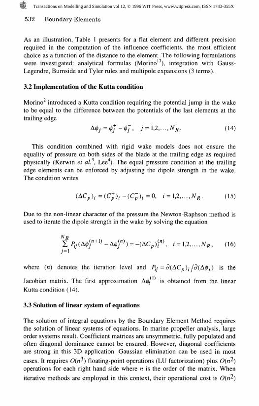
The influence of using flat or hyperboloidal elements has been investigated forthe model problem of a hyperboloid of revolution in a uniform onset flow forwhich analytical solutions are known (Lamb**). A hyberboloid of revolution

(x* +;y^)/(fl^cos^a)-z^ /(c^cot^a) = l with a I c = 0.05 and a = n 14

has been selected. The elements are defined by the intersection of two familiesof rectilinear generators as shown in Figure 2 a). In this case the discretizationof the geometry with hyperboloidal elements is exact. The error is only due tothe approximation of the singularity distributions and the truncation of thesurface of the hyperboloid at a finite distance from the center.

Figure 2 shows the results of calculations of the surface potential for threedifferent discretizations using both flat and hyperboloidal elements. Thenumerical solution converges to the analytical solution (hyperboloid of infinitelength) for small values of the axial coordinate z/c where the error introducedby the finite length of the hyperboloid is negligible. At the plane z / c = 0 theresults for all cases fully agree with the analytical solution. As expected the useof hyperboloidal panels improves the convergence of the results.



1.0

0.5-

o.o

-0.5

-1.0

AnalyticHyp. 12a 72cHat 12a 72c_JHyp. 80 48cFlat 80 48cHyp. 4a 24cFlat4o24c

-0.04 -0.02 0.00

x/c

b)

0.02 0.04

0.80

0.75

0.70

0.65

0.60

Analytico Hyp. 12o72c& Flat 12o72c+ Hyp. 8a48c% Hot 8a48co Hyp. 4a 24c* Hot 4a24c

a)

-0.250 -0.125 0.000 0.125 0.250

z/c

c)

Figure 2: Hyperboloid of revolution, a) Hyperboloid discretization byhyperboloid elements, defined as the intersections of the two families ofrectilinear generators, b) Surface potential along the equatorial circumference atz I c = 0. c) Surface potential along the upstream meridian line in the xz plane.(Symbols a and c indicate axial and circumferential directions respectively).



4.2 Propeller calculations

Calculations were performed for the DTRC4119 propeller at design conditionJ = nU/QRp =0.833. The geometry of the propeller can be found in

Koyama^. Due to the propeller symmetry only one blade and thecorresponding hub sector is used in the solution of the discretized system. Thewake was assumed rigid and helicoidal with pitch equal to the propellergeometric pitch. The wake extends downstream to an axial distance of about 3propeller radius. Figure 3 shows the element arrangement of a finediscretization (60c x 30s) of the propeller with hub and wake. The symbol60cx 30s indicates that the number of elements chordwise is 60 and spanwise30.

Figure 3: Typical surface grid on propeller DTRC4119 showing the wake ofone propeller blade. Total number of elements on one blade and one hub sector:N=2152. Number of elements on the wake: 1650.

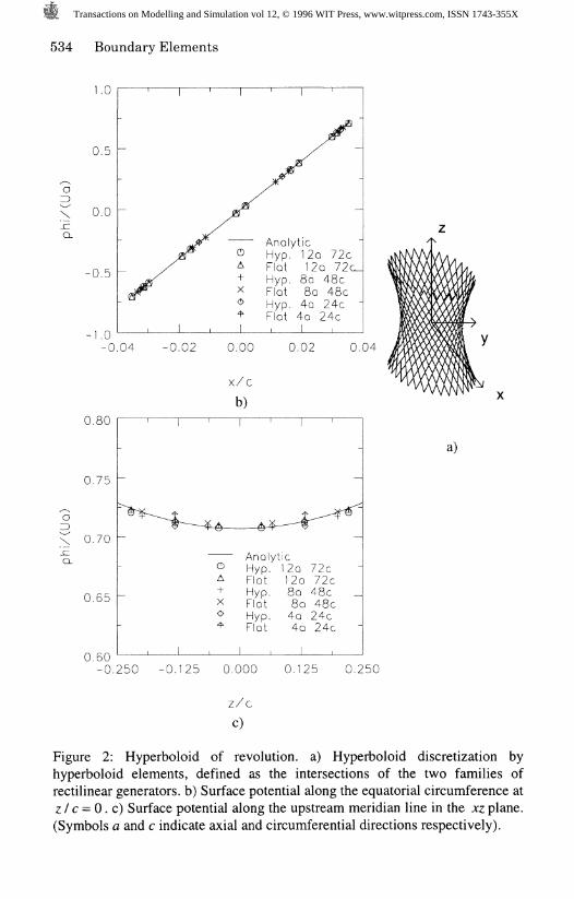
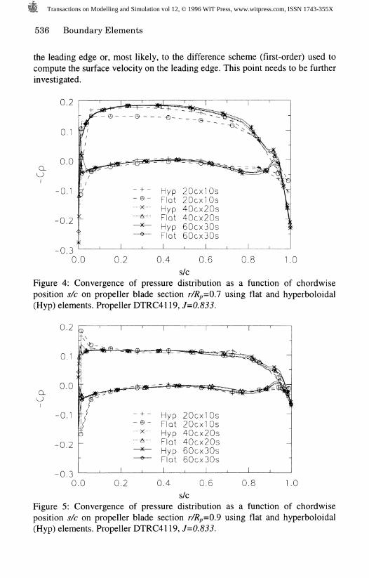
The effect of using flat or hyperboloidal panels in the convergence of themethod was investigated with a grid refinement study. Three different gridswere used with 20cx 10s, 40cx20s and 60cx30s, elements on one blade,respectively. Figures 4 and 5 show the convergence of the pressure distributionfor the blade sections r/Rp=0.1 and r// =0.9, respectively. The results with flatand hyperboloidal elements for the two finest grids are virtually identical withexception of the leading and trailing edge regions. In both cases the results withthe coarser grid have not yet converged. The comparison between the results offlat and hyperboloidal panels shows that the differences are not significant forthe two finest discretizations. However, the use of hyperboloidal elementsconsiderably improves the results of the coarser grid. There is an oscillation ofthe pressure distribution at the first element both on the pressure and suctionsides in all cases. This may be due to the smoothness of the input geometry of



the leading edge or, most likely, to the difference scheme (first-order) used tocompute the surface velocity on the leading edge. This point needs to be furtherinvestigated.

Q_

0.2

0.1

0.0

-0.1

-c .irrfe

?

-0.2 '

-0.3

- + - Hyp 20cx10s-®- Flot20oxlOs^ Hyp 40cx20s^ Flat 40cx20s

-^— Hyp 60ox30s—^- Flat 60cx30s

0.0 0.2 0.4 I.O

s/cFigure 4: Convergence of pressure distribution as a function of chordwiseposition s/c on propeller blade section r/Rp=0.1 using flat and hyperboloidal(Hyp) elements. Propeller DTRC41 19, J=0.833.

CL

0.2

0.1

0.0

-0.

-0.2

-0.3

- Hyp 20oxlOs'- Flat 20cxlOs

Hyp 40ox20sFlat 40cx20s

— Hyp 60cx30s— Flat 60ox30s

0.0 0.2 0.4 0.6 1.0s/c

Figure 5: Convergence of pressure distribution as a function of chordwiseposition s/c on propeller blade section r/Rp=0.9 using flat and hyperboloidal(Hyp) elements. Propeller DTRC41 19, J=0.833.



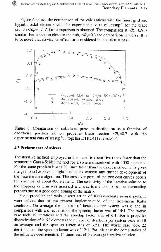
Figure 6 shows the comparison of the calculations with the finest grid andhyperboloidal elements with the experimental data of Jessup^ for the bladesection r/Rp=0.1. A fair comparison is obtained. The comparison at r/Rp=0.9 issimilar. For a section close to the hub, r/Rp=0.3 the comparison is worse. It isto be noted that no viscous effects are considered in the calculations.

Q_O

I

0.0

-0.2

-0.3

Present Method (Hyp 60cx30s)Measured, Press. SideMeasured, Suet. Side

0.0 0.2 O.f 1.00.4- 0.6

s/cFigure 6: Comparison of calculated pressure distribution as a function ofchordwise position s/c on propeller blade section r/Rp=Q.l with theexperimental data of Jessup . Propeller DTRC4119, J=0.833.

4.3 Performance of solvers

The iterative method employed in this paper is about five times faster than thesymmetric Gauss-Seidel method for a sphere discretized with 1000 elements.For the same problem it was 20 times faster than the direct method. This givesmargin to solve several right-hand-sides without any further development ofthe base iterative algorithm. The crossover point of the two cost curves occursfor a number of about 400 elements. The sensitivity of the iterative solution tothe stopping criteria was assessed and was found not to be too demandingperhaps due to a good conditioning of the matrix.

For a propeller and wake discretization of 1080 elements several systemswere solved due to the present implementation of the non-linear Kuttacondition. On average the number of iterations per system was 8 and incomparison with a direct method the speedup factor was of 14:1. The worsecase took 19 iterations and the speedup factor was of 6:1. For a propellerdiscretization of 2152 elements the number of iterations per system were still 8on average and the speedup factor was of 32:1. The worse case took 22iterations and the speedup factor was of 12:1. For this case the computation ofthe influence coefficients is 14 times that of the average iterative solution.



5 Conclusion

This article reports on the current status of the application of a boundaryelement method under development at MARETEC/IST to the computation ofpotential flow around marine propellers. From the work presented here it maybe concluded that the use of hyperboloidal elements significantly improves theconvergence of the numerical solution in comparison with the use of flatelements both for the cases of a hyperboloidal of revolution and the selectedpropeller case. This is in agreement with the results in the literature althoughthe differences encountered for this propeller are not particularly large. Thegrid refinement study performed for the propeller indicates that theintermediate discretization would be sufficient for practical purposes. For thelevel of discretization required by a typical propeller application the iterativesolver employed in this paper shows considerable reductions of CPU time withrespect to the use of a direct method and a Gauss-Seidel iteration.

Acknowledgment

The second author wishes to acknowledge the financial support by PRAXISXXI.

References

1. Hess, J.L. & Valarezo, W.O. Calculation of steady flow about propellersusing a surface panel method, /. Propulsion, 1985, 6, 470-476.

2. Morino, L. & Kuo, C.-C. Subsonic potential aerodynamics for complexconfigurations: A general theory, AIAA Journal, 1974, 12, (2), 191-197.

3. Kerwin, J.E, Kinnas, S.A.,Lee, J-T & Shih, W-Z, A surface panel method forthe hydrodynamic analysis of ducted propellers, 1987, Trans. SNAME, 95.

4. Lee, J-T, A Potential Based Panel Method for the Analysis of MarinePropellers in Steady Flow, Ph.D. thesis, MIT, Department of OceanEngineering, 1987.

S.Hoshino, T., Hydrodynamic analysis of propellers in steady flow using asurface panel method. Journal of the Society of Naval Architects of Japan,1989,165, 55-70.

6. Kinnas, S.A., Hsin, C-Y. & Keenan, D.P., A potential based panel methodfor the unsteady flow around open and ducted propellers, in Proceedings of theEighteenth Symposium on Naval Hydrodynamics, pp 667-685, Ann Arbor,Michigan, August 1990.

7. Hsin, C-Y, Development and Analysis of Panel Method of Propellers inUnsteady Flow, Ph.D. thesis, MIT, Department of Ocean Engineering, 1990.



8. Koyama , K., Application of a panel method for the unsteady hydrodynamicanalysis of marine propellers, in Proceedings of the Nineteenth Symposium onNaval Hydrodynamics, pp 817-836, Seoul, Korea, August 1992.

9. Hoshino, T., Hydrodynamic analysis of propellers in unsteady flow using asurface panel method. Journal of the Society of Naval Architects of Japan,1993,174,71-87.

10. Koyama, K. (ed.). Comparative calculations of propellers by surface panelmethod - Workshop organized by 20* ITTC Propulsor Committee, Papers ofthe Ship Research Institute, Supplement No. 15, September 1993.

11. Romate, I.E. Local error analysis in 3-D panel methods, Journal ofEngineering Mathematics, 1988,22, 123-142.

12. Newman, J.N. Distributions of sources and normal dipoles over aquadrilateral panel, Journal of Engineering Mathematics, 1986, 20, 113-126.

13. Morino, L., Chen, L-T & Suciu, E.G. Steady and oscillatory subsonic andsupersonic aerodynamics around complex configurations, AIAA Journal, 197513, (3), 368-374.

14. Clark, R. W. A new iterative matrix solution procedure for three-dimensional panel methods, AIAA-85-0176, Jan 1985.

15. Sonneveld, P. CGS, a Fast Lanczos-type solver for nonsymmetric linearsystems, SIAM J. Sci. Stat. Comp., 1989,10, (1), pp 36-52.

16. Koruthu, S. P., Conjugate Gradient Squared algorithm for panel methods,AIAA Journal, 1995, 33, (12), pp 2420-2422.

17. van der Vorst, H. A., Bi-CGStab: a fast and smoothly converging variant ofBi-CG for the solution of non-symmetric linear systems, SIAM / Sci. Stat.Comp., 1992, 13, (2), pp 631-644.

18. Eisenstat, S. C., Efficient implementation of a class of Conjugate Gradientmethods, 1981, SIAM /. ScL Stat. Comp., 2, pp 1-4.

19. Lamb, H., Hydrodynamics, Sixth Edition, Cambridge at the UniversityPress, 1962.

20. Jessup, S.D., An Experimental Investigation of Viscous Aspects ofPropeller Blade Flow, Ph.D. thesis, The Catholic Univ. of America, 1989.


Boundary Element Method to the potential flow around ...

Documents

Transcript of Boundary Element Method to the potential flow around ...