BOUNDARY CONDITIONS AND PARTICLES - CSE-Lab
95
BOUNDARY CONDITIONS AND PARTICLES Wednesday, February 25, 2009
Transcript of BOUNDARY CONDITIONS AND PARTICLES - CSE-Lab

BOUNDARY CONDITIONS AND PARTICLESWednesday, February 25, 2009

BOUNDARY CONDITIONS AND PARTICLESWednesday, February 25, 2009

25 years DINFKwww.cse-lab.ethz.chSIMULATIONS USING PARTICLES
Why boundary conditions are important and difficult to treat
BOUNDARY CONDITIONS
Wednesday, February 25, 2009

25 years DINFKwww.cse-lab.ethz.chSIMULATIONS USING PARTICLES
Why boundary conditions are important and difficult to treat
BOUNDARY CONDITIONS
Wednesday, February 25, 2009

25 years DINFKwww.cse-lab.ethz.chSIMULATIONS USING PARTICLES
Boundary conditions and particle methods : a non-standard issue, because particles make sense only as a collection of overlapping points.
A single particle on a boundary not enough to enforce a given boundary condition at that point.
BC for Graphics and CFD
Wednesday, February 25, 2009
25 years DINFKwww.cse-lab.ethz.chSIMULATIONS USING PARTICLES
IMPORTANT to allow the flow to :
Boundary conditions and particle methods : a non-standard issue, because particles make sense only as a collection of overlapping points.
A single particle on a boundary not enough to enforce a given boundary condition at that point.
BC for Graphics and CFD
Wednesday, February 25, 2009

25 years DINFKwww.cse-lab.ethz.chSIMULATIONS USING PARTICLES
IMPORTANT to allow the flow to :
•leave the computational box without non-physical artifacts (numerical issue)
Boundary conditions and particle methods : a non-standard issue, because particles make sense only as a collection of overlapping points.
A single particle on a boundary not enough to enforce a given boundary condition at that point.
BC for Graphics and CFD
Wednesday, February 25, 2009
25 years DINFKwww.cse-lab.ethz.chSIMULATIONS USING PARTICLES
IMPORTANT to allow the flow to :
•leave the computational box without non-physical artifacts (numerical issue)
•inject material in computational box
Boundary conditions and particle methods : a non-standard issue, because particles make sense only as a collection of overlapping points.
A single particle on a boundary not enough to enforce a given boundary condition at that point.
BC for Graphics and CFD
Wednesday, February 25, 2009

25 years DINFKwww.cse-lab.ethz.chSIMULATIONS USING PARTICLES
IMPORTANT to allow the flow to :
•leave the computational box without non-physical artifacts (numerical issue)
•inject material in computational box•generate vorticity and to impart forces at interfaces/solid boundaries (fluid-structure interaction, physical and numerical issue)
Boundary conditions and particle methods : a non-standard issue, because particles make sense only as a collection of overlapping points.
A single particle on a boundary not enough to enforce a given boundary condition at that point.
BC for Graphics and CFD
Wednesday, February 25, 2009

25 years DINFKwww.cse-lab.ethz.chSIMULATIONS USING PARTICLES
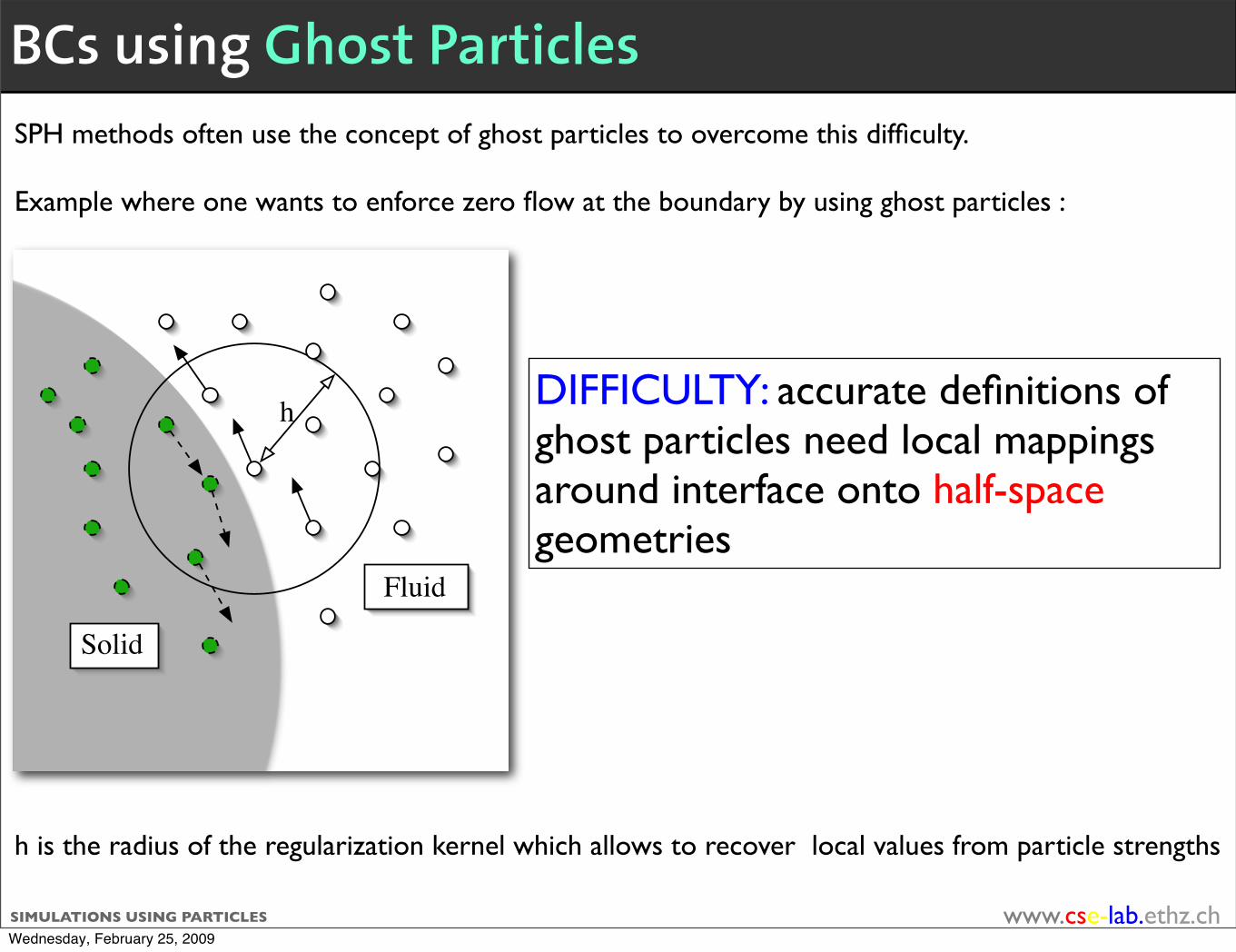
SPH methods often use the concept of ghost particles to overcome this difficulty.
Example where one wants to enforce zero flow at the boundary by using ghost particles :
h
Fluid
Solid
h is the radius of the regularization kernel which allows to recover local values from particle strengths
BCs using Ghost Particles
Wednesday, February 25, 2009
25 years DINFKwww.cse-lab.ethz.chSIMULATIONS USING PARTICLES
SPH methods often use the concept of ghost particles to overcome this difficulty.
Example where one wants to enforce zero flow at the boundary by using ghost particles :
h
Fluid
Solid
h is the radius of the regularization kernel which allows to recover local values from particle strengths
DIFFICULTY: accurate definitions of ghost particles need local mappings around interface onto half-space geometries
BCs using Ghost Particles
Wednesday, February 25, 2009

25 years DINFKwww.cse-lab.ethz.chSIMULATIONS USING PARTICLES
The case of vortex methods for incompressible flows even more delicate, because vorticity boundary values in general not known.
BCs for Vortex Methods
Wednesday, February 25, 2009
25 years DINFKwww.cse-lab.ethz.chSIMULATIONS USING PARTICLES
The case of vortex methods for incompressible flows even more delicate, because vorticity boundary values in general not known.
Like for all numerical methods, can deal with boundary conditions in two ways:
BCs for Vortex Methods
Wednesday, February 25, 2009

25 years DINFKwww.cse-lab.ethz.chSIMULATIONS USING PARTICLES
The case of vortex methods for incompressible flows even more delicate, because vorticity boundary values in general not known.
Like for all numerical methods, can deal with boundary conditions in two ways:•using body-fitted grids (the boundary is made of specific points of a given grid used to solve for the flow)
•seeing the boundary as an immersed boundary
BCs for Vortex Methods
Wednesday, February 25, 2009

25 years DINFKwww.cse-lab.ethz.chSIMULATIONS USING PARTICLES
Boundary conditions appear at two levels:
•KINEMATICS : velocity from vorticity : div u = 0, curl u = ω in Ω and u.n = 0 on ∂Ω (no-through condition)
•DYNAMICS : advection-diffusion equation for vorticity : in Ω , ω = ? on ∂Ω
T(γ(s, t), t) = λ(‖γs(s, t)‖ − 1)
−div(F (ψ, ∇ψ)∇ψ ⊗∇ψ)
(ut + (u · ∇)u) − div σ(ψ,Du,X, ∇X) + ∇p = 0
σ(ψ,Du,X, ∇X) = σS(X, ∇Xt∇X) + H(ψ/ε)
(
σF (Du) − σS(X, ∇Xt∇X)
)
ut + (u · ∇)u − ν∆u + ∇p = λ(u − u)χS
ωt + (u · ∇)ω = (ω · ∇)u + ν∆ω + λ(ω − ω)χS + λ(u − u) × n δ∂S
ωt + (u · ∇)ω = (ω · ∇)u + ν∆ω + (ω − ω)H(ϕ/ε) − (u − u) × ∇ϕ ζε(ϕ)
α4 = γ(Z)
∂φ
∂t+ (u · ∇)φ = 0
ρ
(
∂u
∂t+ (u · ∇)u
)
+ ∇p − ν∆u = f(φ, ∇φ)
ρ
(
∂u
∂t+ (u · ∇)u
)
+ ∇p = ν∆u + ρg + λχS(u − u) + γFe
λ >> 1 , γ = 0
Xt = u(X(r, s, t), t) =
∫
u(x, t)δ(x − X(r, s, t)) dx
f(x, t) =
∫
F(r, s, t)δ(x − X(r, s, t) drds
τ =V
4
3π
(
A4π
)3/2∈ [0, 1]
Ec(φ) =
∫
G(κ(φ))|∇φ|1
εζ
(
φ
ε
)
4
u=0u ! u
!u ! u
!
"f
"s
∂ω
∂t+ (u ·∇)ω = (ω ·∇)u + ν∆ω
Vorticity BCs for No-slip Incompressible Flows
Wednesday, February 25, 2009

25 years DINFKwww.cse-lab.ethz.chSIMULATIONS USING PARTICLES
Classical way to deal with the first boundary condition (u.n = 0 on ∂Ω) is to look for a decomposition of the velocity field into a rotational and a potential part:
u = ∇ φ + ∇ x ψ
Kinematic Boundary Condition
IN PRACTICE : compute first ω, without bothering about boundary conditions, then fix boundary conditions with φ
Wednesday, February 25, 2009

25 years DINFKwww.cse-lab.ethz.chSIMULATIONS USING PARTICLES
div u =0 ⇒ ∆ φ =0 in Ω
Classical way to deal with the first boundary condition (u.n = 0 on ∂Ω) is to look for a decomposition of the velocity field into a rotational and a potential part:
u = ∇ φ + ∇ x ψ
Kinematic Boundary Condition
IN PRACTICE : compute first ω, without bothering about boundary conditions, then fix boundary conditions with φ
Wednesday, February 25, 2009

25 years DINFKwww.cse-lab.ethz.chSIMULATIONS USING PARTICLES
div u =0 ⇒ ∆ φ =0 in Ω∇ x u = ω ⇒ ∆ ψ = ω , div ψ = 0 in Ω.
Boundary Condition u.n =0 gives ∂φ/∂n=-∂(∇xψ)/∂n on ∂Ω
Classical way to deal with the first boundary condition (u.n = 0 on ∂Ω) is to look for a decomposition of the velocity field into a rotational and a potential part:
u = ∇ φ + ∇ x ψ∂U
∂t+ div (a : U) + AU = F
∂(ajui) / ∂xj
ρ(x) =∑
p
αpδ(x − xp)
ρu(x) =∑
p
βp(t)δ(x − xp)
ρE(x) = · · ·
ui =1
εd
∑
p
φi(xp)
u(x) =
∫
Ωf
K(x − y)ω(y) dy +
∫
∂Ω
∇G(x − y)q(y) dy
∂ρ
∂t+
∂(ρu)
∂x= 0
∂(ρu)
∂t+
∂(ρu u)
∂x=
∂p
∂x∂(ρE)
∂t+
∂(ρE u)
∂x=
∂(pu)
∂x
Comparison with a recent work of Smereka about approximation of delta-functions: computation of thearc-length of an ellipse
φ(x, y) =x2
a2+
y2
b2− 1 L =
∫
Ω
1
εζ(
φ
ε)|∇ϕ|dxdy
with a = 1.5 and b = 0.75, with random center and orientation.
Mesh Size Smereka RenormalizationRel. Error Order Rel. Error Order
0.2 9.38 × 10⁻³ 1.5 × 10⁻¹
0.1 2.23 × 10⁻³ 2.07 5 × 10⁻³
0.05 8.12 × 10⁻⁴ 1.46 1.3 × 10⁻³ 1.90.025 2.71 × 10⁻⁴ 1.58 3 × 10⁻⁴ 2.110.0125 7.58 × 10⁻⁵ 1.83 8 × 10⁻⁵ 1.90.00625 3.04 × 10⁻⁵ 1.32 2 × 10⁻⁵ 2
∂ω
∂t+ (u · ∇)ω − (ω · ∇)u = 0 in fluid domain (1)
u · n = 0 on Γb (2)
∂ω
∂t− ν∆ω = 0 in fluid domain
ν∂ω
∂n= −
u · τ
∆ton Γb
1
where q is a potential to be determined from an integral equation on ∂Ω
In a grid-free vortex method, this results in :
Kinematic Boundary Condition
IN PRACTICE : compute first ω, without bothering about boundary conditions, then fix boundary conditions with φ
Wednesday, February 25, 2009

25 years DINFKwww.cse-lab.ethz.chSIMULATIONS USING PARTICLES
Next, enforce that tangential velocities are also zero at the boundary
traditional numerical recipe for vortex methods mimics the physical mechanism: vorticity produced at the boundary to prevent any slip velocity at the boundary
DYNAMICS - No-slip Condition
Wednesday, February 25, 2009

25 years DINFKwww.cse-lab.ethz.chSIMULATIONS USING PARTICLES
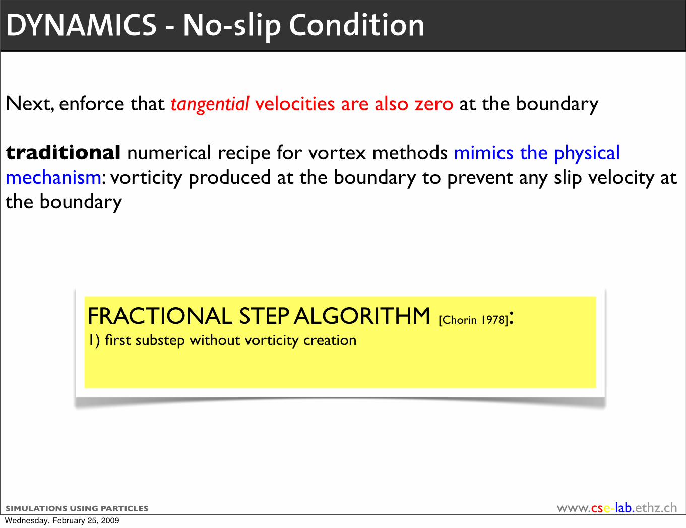
Next, enforce that tangential velocities are also zero at the boundary
traditional numerical recipe for vortex methods mimics the physical mechanism: vorticity produced at the boundary to prevent any slip velocity at the boundary
FRACTIONAL STEP ALGORITHM [Chorin 1978]:
DYNAMICS - No-slip Condition
Wednesday, February 25, 2009
25 years DINFKwww.cse-lab.ethz.chSIMULATIONS USING PARTICLES
Next, enforce that tangential velocities are also zero at the boundary
traditional numerical recipe for vortex methods mimics the physical mechanism: vorticity produced at the boundary to prevent any slip velocity at the boundary
FRACTIONAL STEP ALGORITHM [Chorin 1978]: 1) first substep without vorticity creation
DYNAMICS - No-slip Condition
Wednesday, February 25, 2009

25 years DINFKwww.cse-lab.ethz.chSIMULATIONS USING PARTICLES
Next, enforce that tangential velocities are also zero at the boundary
traditional numerical recipe for vortex methods mimics the physical mechanism: vorticity produced at the boundary to prevent any slip velocity at the boundary
FRACTIONAL STEP ALGORITHM [Chorin 1978]: 1) first substep without vorticity creation2) compute resulting slip
DYNAMICS - No-slip Condition
Wednesday, February 25, 2009

25 years DINFKwww.cse-lab.ethz.chSIMULATIONS USING PARTICLES
Next, enforce that tangential velocities are also zero at the boundary
traditional numerical recipe for vortex methods mimics the physical mechanism: vorticity produced at the boundary to prevent any slip velocity at the boundary
FRACTIONAL STEP ALGORITHM [Chorin 1978]: 1) first substep without vorticity creation2) compute resulting slip3) remove this slip by injecting in the flow the appropriate sheet of vorticity
DYNAMICS - No-slip Condition
Wednesday, February 25, 2009

25 years DINFKwww.cse-lab.ethz.chSIMULATIONS USING PARTICLES
Next, enforce that tangential velocity are also zero at the boundary
traditional numerical recipe for vortex methods mimics the physical mechanism: vorticity produced at the boundary to prevent any slip velocity at the boundary
[Koumoutsakos-Leonard 1992]
DYNAMICS - Lighthill’s Algorithm
Wednesday, February 25, 2009
25 years DINFKwww.cse-lab.ethz.chSIMULATIONS USING PARTICLES
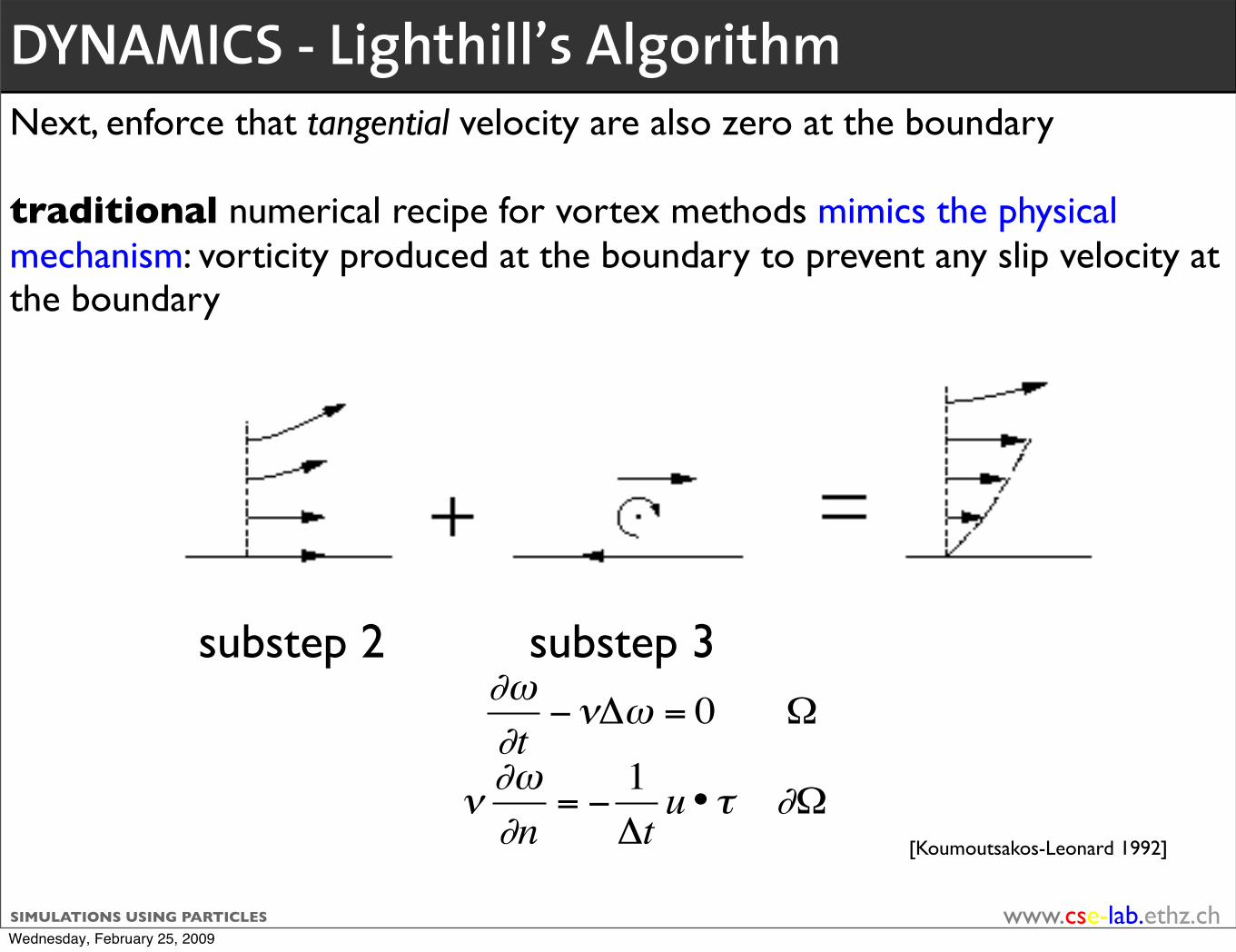
Next, enforce that tangential velocity are also zero at the boundary
traditional numerical recipe for vortex methods mimics the physical mechanism: vorticity produced at the boundary to prevent any slip velocity at the boundary
substep 2 substep 3
€
∂ω∂t
−νΔω = 0 Ω
ν∂ω∂n
= −1Δtu•τ ∂Ω
[Koumoutsakos-Leonard 1992]
DYNAMICS - Lighthill’s Algorithm
Wednesday, February 25, 2009

25 years DINFKwww.cse-lab.ethz.chSIMULATIONS USING PARTICLES
In 3D, need boundary conditions for 3 vorticity components
=
After advection step computation of slip
Vorticity flux onto flow particles
+
case of flow past a cylinder[Cottet-Poncet 2003]
3D Vorticity Flux BCs
Wednesday, February 25, 2009
25 years DINFKwww.cse-lab.ethz.chSIMULATIONS USING PARTICLES
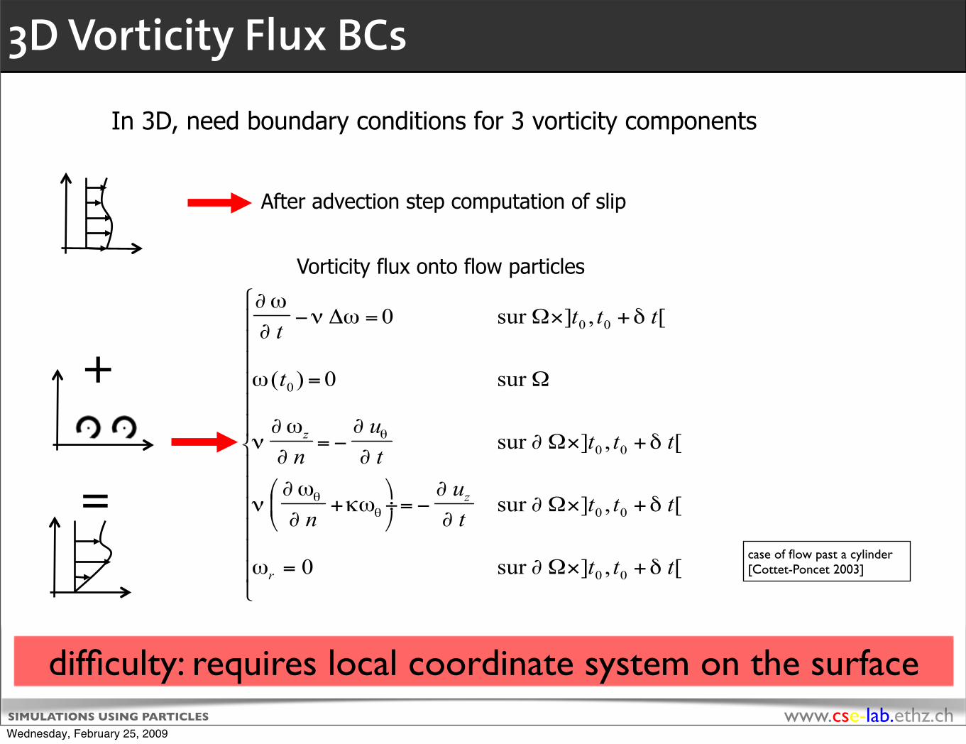
In 3D, need boundary conditions for 3 vorticity components
=
After advection step computation of slip
Vorticity flux onto flow particles
+
difficulty: requires local coordinate system on the surface
case of flow past a cylinder[Cottet-Poncet 2003]
3D Vorticity Flux BCs
Wednesday, February 25, 2009

25 years DINFKwww.cse-lab.ethz.chSIMULATIONS USING PARTICLES
u=0u=u
!u=u
!
"f
"s
The case of a rigid body with prescribed velocity
Obstacles, walls, objects .. are part of the flow, with specific rheology
IMMERSED BOUNDARIES
Wednesday, February 25, 2009

25 years DINFKwww.cse-lab.ethz.chSIMULATIONS USING PARTICLES
•rigid body with prescribed velocity or interacting with flow
u=0u=u
!u=u
!
"f
"s
The case of a rigid body with prescribed velocity
Obstacles, walls, objects .. are part of the flow, with specific rheology
IMMERSED BOUNDARIES
Wednesday, February 25, 2009

25 years DINFKwww.cse-lab.ethz.chSIMULATIONS USING PARTICLES
•rigid body with prescribed velocity or interacting with flow•elastic membrane
u=0u=u
!u=u
!
"f
"s
The case of a rigid body with prescribed velocity
Obstacles, walls, objects .. are part of the flow, with specific rheology
IMMERSED BOUNDARIES
Wednesday, February 25, 2009

25 years DINFKwww.cse-lab.ethz.chSIMULATIONS USING PARTICLES
•rigid body with prescribed velocity or interacting with flow•elastic membrane•visco-elastic body ..
u=0u=u
!u=u
!
"f
"s
The case of a rigid body with prescribed velocity
Obstacles, walls, objects .. are part of the flow, with specific rheology
IMMERSED BOUNDARIES
Wednesday, February 25, 2009
25 years DINFKwww.cse-lab.ethz.chSIMULATIONS USING PARTICLES
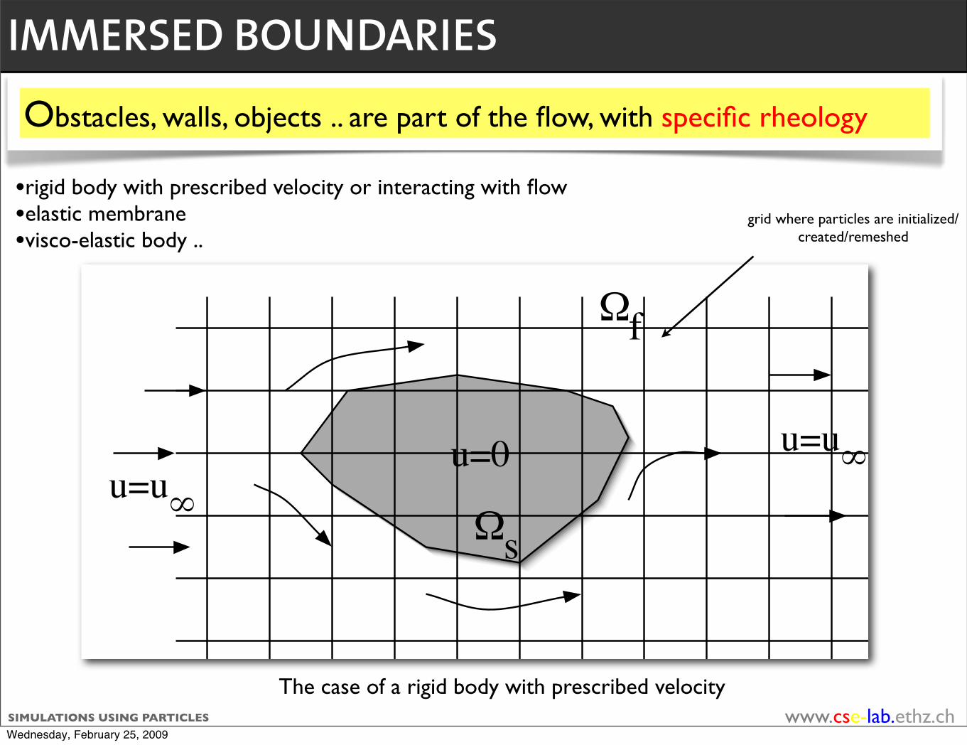
•rigid body with prescribed velocity or interacting with flow•elastic membrane•visco-elastic body ..
u=0u=u
!u=u
!
"f
"s
The case of a rigid body with prescribed velocity
Obstacles, walls, objects .. are part of the flow, with specific rheology
grid where particles are initialized/created/remeshed
IMMERSED BOUNDARIES
Wednesday, February 25, 2009

25 years DINFKwww.cse-lab.ethz.chSIMULATIONS USING PARTICLES
Boundary Conditions = Coupling Dynamics
Boundary Conditions
Wednesday, February 25, 2009

25 years DINFKwww.cse-lab.ethz.chSIMULATIONS USING PARTICLES
Boundary Conditions = Coupling Dynamics
Boundary Conditions
Wednesday, February 25, 2009

25 years DINFKwww.cse-lab.ethz.chSIMULATIONS USING PARTICLES
Boundary Conditions = Coupling Dynamics
• Coupling via a Boundary Force
Boundary Conditions
Wednesday, February 25, 2009
25 years DINFKwww.cse-lab.ethz.chSIMULATIONS USING PARTICLES
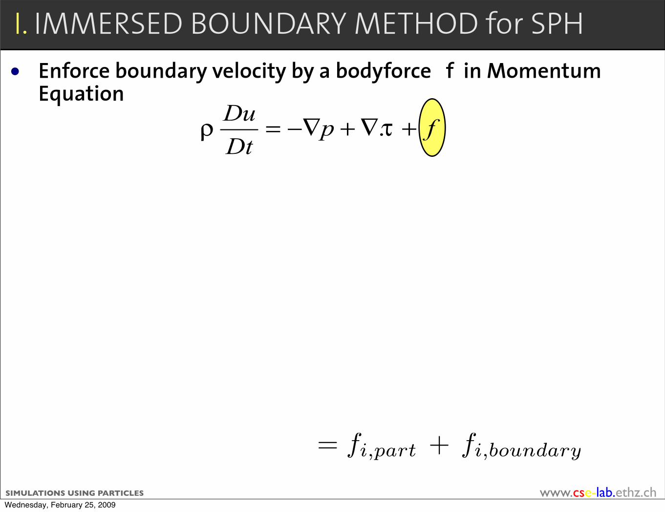
• Enforce boundary velocity by a bodyforce f in Momentum Equation
I. IMMERSED BOUNDARY METHOD for SPH
= fi,part + fi,boundary
Wednesday, February 25, 2009

25 years DINFKwww.cse-lab.ethz.chSIMULATIONS USING PARTICLES
• Enforce boundary velocity by a bodyforce f in Momentum Equation
I. IMMERSED BOUNDARY METHOD for SPH
• Approximate Material Derivative at time step i and solve for f
• Desired Velocity field on the boundary
= fi,part + fi,boundary
Wednesday, February 25, 2009

25 years DINFKwww.cse-lab.ethz.chSIMULATIONS USING PARTICLES
Boundary Conditions : A Particle-Mesh Operation
Wednesday, February 25, 2009

25 years DINFKwww.cse-lab.ethz.chSIMULATIONS USING PARTICLES
Boundary Conditions : A Particle-Mesh Operation
• Compute part of forcing term on the particles
Wednesday, February 25, 2009

25 years DINFKwww.cse-lab.ethz.chSIMULATIONS USING PARTICLES
Boundary Conditions : A Particle-Mesh Operation
• Compute part of forcing term on the particles
• Particles to Boundary (Particle to Mesh Interpolation)
Wednesday, February 25, 2009

25 years DINFKwww.cse-lab.ethz.chSIMULATIONS USING PARTICLES
Boundary Conditions : A Particle-Mesh Operation
• Compute part of forcing term on the particles
• Particles to Boundary (Particle to Mesh Interpolation)
• Force -> Boundary to Particles (Mesh - Particle Interpolation)
Wednesday, February 25, 2009

25 years DINFKwww.cse-lab.ethz.chSIMULATIONS USING PARTICLES
Boundary Conditions : A Particle-Mesh Operation
• Compute part of forcing term on the particles
• Particles to Boundary (Particle to Mesh Interpolation)
S. Hieber and PK., Immersed Boundary Method for SPH, J. Comp. Physics, 2008A. Dupuis, P. Chatelain, and PK., Coupling lattice Boltzmann and molecular dynamics for dense fluids. Phys. Rev. E, 75: 046704, 2007
• Force -> Boundary to Particles (Mesh - Particle Interpolation)
Wednesday, February 25, 2009

25 years DINFKwww.cse-lab.ethz.chSIMULATIONS USING PARTICLES
Lattice Boltzmann and Impulsively Started Cylinders
A. Dupuis, P. Chatelain, PK, An immersed boundary–lattice-Boltzmann method for the simulation of the flow past an impulsively started cylinder, J. Computational Physics, 227, 2008
Wednesday, February 25, 2009
25 years DINFKwww.cse-lab.ethz.chSIMULATIONS USING PARTICLES
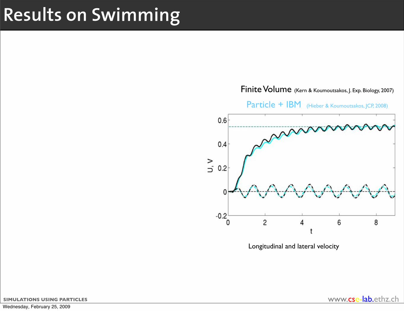
Results on Swimming
Longitudinal and lateral velocity
Finite Volume (Kern & Koumoutsakos, J. Exp. Biology, 2007)
Particle + IBM (Hieber & Koumoutsakos, JCP, 2008)
Wednesday, February 25, 2009
25 years DINFKwww.cse-lab.ethz.chSIMULATIONS USING PARTICLES
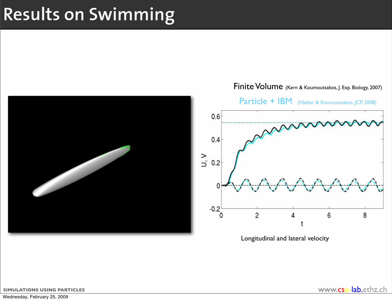
Results on Swimming
Longitudinal and lateral velocity
Finite Volume (Kern & Koumoutsakos, J. Exp. Biology, 2007)
Particle + IBM (Hieber & Koumoutsakos, JCP, 2008)
Wednesday, February 25, 2009

25 years DINFKwww.cse-lab.ethz.chSIMULATIONS USING PARTICLES
One way to view/derive immersed boundary techniques based on a penalized flow equation [Angot-Bruneau-Fabrie 1999]
58
Obstacle
Fluid
Tagged grid points for
the solution
of the linear system
Physical boundaryNumerical
boundary
Figure 35: Immersed boundary
6.2.3 IMMERSED BOUNDARY TECHNIQUES - THE PENALIZATION METHOD Theidea behind penalization method is to view obstacles, walls, etc .. as porous mediawhich absorb the velocity in a small layer on the boundary of the obstacle [2]. From amathematical point of view, it means assuming a flow everywhere, including inside theobstacles, and adding a term in the flow equation which drives the velocity back to zero- or whatever value is sought - inside the obstacles.
To be more specific, we consider, in a computational domain K, the case of an incom-pressible flow around an object S with prescribed velocity u inside S. We denote by λa penalization parameter, λ >> 1, and denote by χS the characteristic function of S (1inside, 0 outside). The model equation is then the following :
ρ
(∂u
∂t+ (u ·∇)u
)− ν∆u +∇p = ρ g + λ ρχS(u− u)forx ∈ K (92)
coupled with the incompressibility condition
div u = 0 for x ∈ K (93)
In the above equation ρ denotes the density, with value ρS in S and ρF in the fluidoutside S, F = K − S. If we want to use vortex particles to handle this penalizationmodel, we first need to derive the vorticity form of (92). Taking the curl of (92) we get
∂ω
∂t+ (u ·∇)ω = (ω ·∇)u + ν∆ω −∇p×∇(
1ρ) + λ∇×χS(u− u). (94)
This system has to be complemented by the usual system giving the velocity in terms ofthe vorticity :
∇ · u = 0inK;∇×u = ω inK. (95)
The right hand side above exhibits two terms : a so-called barotropic term, resultingfrom the density variations, already seen in variable density and free surface flows, and
In a vorticity formulation, leads to
complemented by the usual system giving u from ω
59
a term coming from the penalization. We now continue with the derivation of the model.Developing the term ∇×χS(u− u) one obtains
∂ω
∂t+(u·∇)ω−(ω ·∇)u−ν∆ω = −∇p×∇(
1ρ)+λχS(ω−ω)+λδΣ n×(u−u). (96)
In the above equation we have set ω = ∇×u and n is the normal to the interface Σ ori-ented towards the solid. It is interesting to note that the right hand side of this equationcontains, in addition to the density-driven term, a vorticity generator coming from theno-slip condition at the fluid-solid interface.This term is also localized at the interface.It is very much reminiscent to vorticity creation algorithms that we have outlined whenwe have discussed gird-free methods (Figure 34). A definite difference though withpreviously seen immersed boundary methods, is that here, both normal and tangentialcomponents of the velocity are handled by a single term in the vorticity equation. Thisgreatly simplifies the algorithm. A drawback is that the condition on the normal compo-nent is possibly not satisfied with the same accuracy as when it is addressed by potentialsources like in 6.2.2. Therefore it may happens that a few particles cross the interface.To avoid circulation defect in the method, it is therefore important that vorticity insidethe solid domain is not discarded. We will outline the algorithm box, when we adressthe more general situation of a fluid fully interacting with a solid body.
6.3 Interaction of a fluid with rigid bodies
The classical approach to adress fluid solid interaction (wether the solid is rigid or elas-tic) is to solve separately fluid and solids, with the associated physics, and to couplethem through interface conditions that translate the continuity of forces and velocities.In general the description of the physics in the fluids is Eulerian, that is equations of thefluid are solved in Eulerian coordinates on a grid, while it is Lagrangian in the solid.The grid for the fluid has to adjust to the moving interface with the solid, at least in thenormal direction (whence the name ALE for Arbitrary Lagrangian Eulerian methods).These methods are rather tricky to implement in particular in 3D and/or in presence oflarge defomations.It is clearly possible to define ALE particle methods, here the fluid issolved by a grid-free or hybrid particle-grid algorithm combined with solid solvers (forinstance based on classical Finite Element solvers). However one may anticipate thatthese methods will face the problems of all ALE methods, with the additional difficultyinherent to particle methods for enforcing boundary conditions.
In the following we therefore focus on an alternative approach, which is to considerfluids and solids as a single, variable density, multiphase, flow. The different phases,fluids, elastic or rigid solids, are captured by level set methods. Interface conditions areenforced by penalization methods. We first consider the case of a single rigid body in anincompressible fluid, and we show how to model it with a vortex particle method
The starting model is the penalization model (94) just seen, with two additional fea-tures:
• the solid velocity is not given, but a result of flow forces, gravity and so on ..• the solid is moving, and its boundary is captured by a level set function.
This means that we have to complement (94) by an expression for u, an advection equa-tion for a level set following the fluid/solid interface, and an expression of the penaliza-
II. IMMERSED BOUNDARY via PENALISATION
Wednesday, February 25, 2009

25 years DINFKwww.cse-lab.ethz.chSIMULATIONS USING PARTICLES
•ū = prescribed body velocity, •χS = 1 in the body, 0 outside and •λ a (large) penalization parameter.
One way to view/derive immersed boundary techniques based on a penalized flow equation [Angot-Bruneau-Fabrie 1999]
58
Obstacle
Fluid
Tagged grid points for
the solution
of the linear system
Physical boundaryNumerical
boundary
Figure 35: Immersed boundary
6.2.3 IMMERSED BOUNDARY TECHNIQUES - THE PENALIZATION METHOD Theidea behind penalization method is to view obstacles, walls, etc .. as porous mediawhich absorb the velocity in a small layer on the boundary of the obstacle [2]. From amathematical point of view, it means assuming a flow everywhere, including inside theobstacles, and adding a term in the flow equation which drives the velocity back to zero- or whatever value is sought - inside the obstacles.
To be more specific, we consider, in a computational domain K, the case of an incom-pressible flow around an object S with prescribed velocity u inside S. We denote by λa penalization parameter, λ >> 1, and denote by χS the characteristic function of S (1inside, 0 outside). The model equation is then the following :
ρ
(∂u
∂t+ (u ·∇)u
)− ν∆u +∇p = ρ g + λ ρχS(u− u)forx ∈ K (92)
coupled with the incompressibility condition
div u = 0 for x ∈ K (93)
In the above equation ρ denotes the density, with value ρS in S and ρF in the fluidoutside S, F = K − S. If we want to use vortex particles to handle this penalizationmodel, we first need to derive the vorticity form of (92). Taking the curl of (92) we get
∂ω
∂t+ (u ·∇)ω = (ω ·∇)u + ν∆ω −∇p×∇(
1ρ) + λ∇×χS(u− u). (94)
This system has to be complemented by the usual system giving the velocity in terms ofthe vorticity :
∇ · u = 0inK;∇×u = ω inK. (95)
The right hand side above exhibits two terms : a so-called barotropic term, resultingfrom the density variations, already seen in variable density and free surface flows, and
58
Obstacle
Fluid
Tagged grid points for
the solution
of the linear system
Physical boundaryNumerical
boundary
Figure 35: Immersed boundary
6.2.3 IMMERSED BOUNDARY TECHNIQUES - THE PENALIZATION METHOD Theidea behind penalization method is to view obstacles, walls, etc .. as porous mediawhich absorb the velocity in a small layer on the boundary of the obstacle [2]. From amathematical point of view, it means assuming a flow everywhere, including inside theobstacles, and adding a term in the flow equation which drives the velocity back to zero- or whatever value is sought - inside the obstacles.
To be more specific, we consider, in a computational domain K, the case of an incom-pressible flow around an object S with prescribed velocity u inside S. We denote by λa penalization parameter, λ >> 1, and denote by χS the characteristic function of S (1inside, 0 outside). The model equation is then the following :
ρ
(∂u
∂t+ (u ·∇)u
)− ν∆u +∇p = ρ g + λ ρχS(u− u)forx ∈ K (92)
coupled with the incompressibility condition
div u = 0 for x ∈ K (93)
In the above equation ρ denotes the density, with value ρS in S and ρF in the fluidoutside S, F = K − S. If we want to use vortex particles to handle this penalizationmodel, we first need to derive the vorticity form of (92). Taking the curl of (92) we get
∂ω
∂t+ (u ·∇)ω = (ω ·∇)u + ν∆ω −∇p×∇(
1ρ) + λ∇×χS(u− u). (94)
This system has to be complemented by the usual system giving the velocity in terms ofthe vorticity :
∇ · u = 0inK;∇×u = ω inK. (95)
The right hand side above exhibits two terms : a so-called barotropic term, resultingfrom the density variations, already seen in variable density and free surface flows, and
58
Obstacle
Fluid
Tagged grid points for
the solution
of the linear system
Physical boundaryNumerical
boundary
Figure 35: Immersed boundary
6.2.3 IMMERSED BOUNDARY TECHNIQUES - THE PENALIZATION METHOD Theidea behind penalization method is to view obstacles, walls, etc .. as porous mediawhich absorb the velocity in a small layer on the boundary of the obstacle [2]. From amathematical point of view, it means assuming a flow everywhere, including inside theobstacles, and adding a term in the flow equation which drives the velocity back to zero- or whatever value is sought - inside the obstacles.
To be more specific, we consider, in a computational domain K, the case of an incom-pressible flow around an object S with prescribed velocity u inside S. We denote by λa penalization parameter, λ >> 1, and denote by χS the characteristic function of S (1inside, 0 outside). The model equation is then the following :
ρ
(∂u
∂t+ (u ·∇)u
)− ν∆u +∇p = ρ g + λ ρχS(u− u)forx ∈ K (92)
coupled with the incompressibility condition
div u = 0 for x ∈ K (93)
In the above equation ρ denotes the density, with value ρS in S and ρF in the fluidoutside S, F = K − S. If we want to use vortex particles to handle this penalizationmodel, we first need to derive the vorticity form of (92). Taking the curl of (92) we get
∂ω
∂t+ (u ·∇)ω = (ω ·∇)u + ν∆ω −∇p×∇(
1ρ) + λ∇×χS(u− u). (94)
This system has to be complemented by the usual system giving the velocity in terms ofthe vorticity :
∇ · u = 0inK;∇×u = ω inK. (95)
The right hand side above exhibits two terms : a so-called barotropic term, resultingfrom the density variations, already seen in variable density and free surface flows, and
In a vorticity formulation, leads to
complemented by the usual system giving u from ω
59
a term coming from the penalization. We now continue with the derivation of the model.Developing the term ∇×χS(u− u) one obtains
∂ω
∂t+(u·∇)ω−(ω ·∇)u−ν∆ω = −∇p×∇(
1ρ)+λχS(ω−ω)+λδΣ n×(u−u). (96)
In the above equation we have set ω = ∇×u and n is the normal to the interface Σ ori-ented towards the solid. It is interesting to note that the right hand side of this equationcontains, in addition to the density-driven term, a vorticity generator coming from theno-slip condition at the fluid-solid interface.This term is also localized at the interface.It is very much reminiscent to vorticity creation algorithms that we have outlined whenwe have discussed gird-free methods (Figure 34). A definite difference though withpreviously seen immersed boundary methods, is that here, both normal and tangentialcomponents of the velocity are handled by a single term in the vorticity equation. Thisgreatly simplifies the algorithm. A drawback is that the condition on the normal compo-nent is possibly not satisfied with the same accuracy as when it is addressed by potentialsources like in 6.2.2. Therefore it may happens that a few particles cross the interface.To avoid circulation defect in the method, it is therefore important that vorticity insidethe solid domain is not discarded. We will outline the algorithm box, when we adressthe more general situation of a fluid fully interacting with a solid body.
6.3 Interaction of a fluid with rigid bodies
The classical approach to adress fluid solid interaction (wether the solid is rigid or elas-tic) is to solve separately fluid and solids, with the associated physics, and to couplethem through interface conditions that translate the continuity of forces and velocities.In general the description of the physics in the fluids is Eulerian, that is equations of thefluid are solved in Eulerian coordinates on a grid, while it is Lagrangian in the solid.The grid for the fluid has to adjust to the moving interface with the solid, at least in thenormal direction (whence the name ALE for Arbitrary Lagrangian Eulerian methods).These methods are rather tricky to implement in particular in 3D and/or in presence oflarge defomations.It is clearly possible to define ALE particle methods, here the fluid issolved by a grid-free or hybrid particle-grid algorithm combined with solid solvers (forinstance based on classical Finite Element solvers). However one may anticipate thatthese methods will face the problems of all ALE methods, with the additional difficultyinherent to particle methods for enforcing boundary conditions.
In the following we therefore focus on an alternative approach, which is to considerfluids and solids as a single, variable density, multiphase, flow. The different phases,fluids, elastic or rigid solids, are captured by level set methods. Interface conditions areenforced by penalization methods. We first consider the case of a single rigid body in anincompressible fluid, and we show how to model it with a vortex particle method
The starting model is the penalization model (94) just seen, with two additional fea-tures:
• the solid velocity is not given, but a result of flow forces, gravity and so on ..• the solid is moving, and its boundary is captured by a level set function.
This means that we have to complement (94) by an expression for u, an advection equa-tion for a level set following the fluid/solid interface, and an expression of the penaliza-
II. IMMERSED BOUNDARY via PENALISATION
Wednesday, February 25, 2009

25 years DINFKwww.cse-lab.ethz.chSIMULATIONS USING PARTICLES
to understand the role of the additional term in the flow equation, useful to extend it
drives vorticity back to the correct body vorticity
creates a vortex sheet on the body surface
59
a term coming from the penalization. We now continue with the derivation of the model.Developing the term ∇×χS(u− u) one obtains
∂ω
∂t+(u·∇)ω−(ω ·∇)u−ν∆ω = −∇p×∇(
1ρ)+λχS(ω−ω)+λδΣ n×(u−u). (96)
In the above equation we have set ω = ∇×u and n is the normal to the interface Σ ori-ented towards the solid. It is interesting to note that the right hand side of this equationcontains, in addition to the density-driven term, a vorticity generator coming from theno-slip condition at the fluid-solid interface.This term is also localized at the interface.It is very much reminiscent to vorticity creation algorithms that we have outlined whenwe have discussed gird-free methods (Figure 34). A definite difference though withpreviously seen immersed boundary methods, is that here, both normal and tangentialcomponents of the velocity are handled by a single term in the vorticity equation. Thisgreatly simplifies the algorithm. A drawback is that the condition on the normal compo-nent is possibly not satisfied with the same accuracy as when it is addressed by potentialsources like in 6.2.2. Therefore it may happens that a few particles cross the interface.To avoid circulation defect in the method, it is therefore important that vorticity insidethe solid domain is not discarded. We will outline the algorithm box, when we adressthe more general situation of a fluid fully interacting with a solid body.
6.3 Interaction of a fluid with rigid bodies
The classical approach to adress fluid solid interaction (wether the solid is rigid or elas-tic) is to solve separately fluid and solids, with the associated physics, and to couplethem through interface conditions that translate the continuity of forces and velocities.In general the description of the physics in the fluids is Eulerian, that is equations of thefluid are solved in Eulerian coordinates on a grid, while it is Lagrangian in the solid.The grid for the fluid has to adjust to the moving interface with the solid, at least in thenormal direction (whence the name ALE for Arbitrary Lagrangian Eulerian methods).These methods are rather tricky to implement in particular in 3D and/or in presence oflarge defomations.It is clearly possible to define ALE particle methods, here the fluid issolved by a grid-free or hybrid particle-grid algorithm combined with solid solvers (forinstance based on classical Finite Element solvers). However one may anticipate thatthese methods will face the problems of all ALE methods, with the additional difficultyinherent to particle methods for enforcing boundary conditions.
In the following we therefore focus on an alternative approach, which is to considerfluids and solids as a single, variable density, multiphase, flow. The different phases,fluids, elastic or rigid solids, are captured by level set methods. Interface conditions areenforced by penalization methods. We first consider the case of a single rigid body in anincompressible fluid, and we show how to model it with a vortex particle method
The starting model is the penalization model (94) just seen, with two additional fea-tures:
• the solid velocity is not given, but a result of flow forces, gravity and so on ..• the solid is moving, and its boundary is captured by a level set function.
This means that we have to complement (94) by an expression for u, an advection equa-tion for a level set following the fluid/solid interface, and an expression of the penaliza-
Vorticity form of PENALISATION
Wednesday, February 25, 2009

25 years DINFKwww.cse-lab.ethz.chSIMULATIONS USING PARTICLES
to understand the role of the additional term in the flow equation, useful to extend it
drives vorticity back to the correct body vorticity
creates a vortex sheet on the body surface
59
a term coming from the penalization. We now continue with the derivation of the model.Developing the term ∇×χS(u− u) one obtains
∂ω
∂t+(u·∇)ω−(ω ·∇)u−ν∆ω = −∇p×∇(
1ρ)+λχS(ω−ω)+λδΣ n×(u−u). (96)
In the above equation we have set ω = ∇×u and n is the normal to the interface Σ ori-ented towards the solid. It is interesting to note that the right hand side of this equationcontains, in addition to the density-driven term, a vorticity generator coming from theno-slip condition at the fluid-solid interface.This term is also localized at the interface.It is very much reminiscent to vorticity creation algorithms that we have outlined whenwe have discussed gird-free methods (Figure 34). A definite difference though withpreviously seen immersed boundary methods, is that here, both normal and tangentialcomponents of the velocity are handled by a single term in the vorticity equation. Thisgreatly simplifies the algorithm. A drawback is that the condition on the normal compo-nent is possibly not satisfied with the same accuracy as when it is addressed by potentialsources like in 6.2.2. Therefore it may happens that a few particles cross the interface.To avoid circulation defect in the method, it is therefore important that vorticity insidethe solid domain is not discarded. We will outline the algorithm box, when we adressthe more general situation of a fluid fully interacting with a solid body.
6.3 Interaction of a fluid with rigid bodies
The classical approach to adress fluid solid interaction (wether the solid is rigid or elas-tic) is to solve separately fluid and solids, with the associated physics, and to couplethem through interface conditions that translate the continuity of forces and velocities.In general the description of the physics in the fluids is Eulerian, that is equations of thefluid are solved in Eulerian coordinates on a grid, while it is Lagrangian in the solid.The grid for the fluid has to adjust to the moving interface with the solid, at least in thenormal direction (whence the name ALE for Arbitrary Lagrangian Eulerian methods).These methods are rather tricky to implement in particular in 3D and/or in presence oflarge defomations.It is clearly possible to define ALE particle methods, here the fluid issolved by a grid-free or hybrid particle-grid algorithm combined with solid solvers (forinstance based on classical Finite Element solvers). However one may anticipate thatthese methods will face the problems of all ALE methods, with the additional difficultyinherent to particle methods for enforcing boundary conditions.
In the following we therefore focus on an alternative approach, which is to considerfluids and solids as a single, variable density, multiphase, flow. The different phases,fluids, elastic or rigid solids, are captured by level set methods. Interface conditions areenforced by penalization methods. We first consider the case of a single rigid body in anincompressible fluid, and we show how to model it with a vortex particle method
The starting model is the penalization model (94) just seen, with two additional fea-tures:
• the solid velocity is not given, but a result of flow forces, gravity and so on ..• the solid is moving, and its boundary is captured by a level set function.
This means that we have to complement (94) by an expression for u, an advection equa-tion for a level set following the fluid/solid interface, and an expression of the penaliza-
59
a term coming from the penalization. We now continue with the derivation of the model.Developing the term ∇×χS(u− u) one obtains
∂ω
∂t+(u·∇)ω−(ω ·∇)u−ν∆ω = −∇p×∇(
1ρ)+λχS(ω−ω)+λδΣ n×(u−u). (96)
In the above equation we have set ω = ∇×u and n is the normal to the interface Σ ori-ented towards the solid. It is interesting to note that the right hand side of this equationcontains, in addition to the density-driven term, a vorticity generator coming from theno-slip condition at the fluid-solid interface.This term is also localized at the interface.It is very much reminiscent to vorticity creation algorithms that we have outlined whenwe have discussed gird-free methods (Figure 34). A definite difference though withpreviously seen immersed boundary methods, is that here, both normal and tangentialcomponents of the velocity are handled by a single term in the vorticity equation. Thisgreatly simplifies the algorithm. A drawback is that the condition on the normal compo-nent is possibly not satisfied with the same accuracy as when it is addressed by potentialsources like in 6.2.2. Therefore it may happens that a few particles cross the interface.To avoid circulation defect in the method, it is therefore important that vorticity insidethe solid domain is not discarded. We will outline the algorithm box, when we adressthe more general situation of a fluid fully interacting with a solid body.
6.3 Interaction of a fluid with rigid bodies
The classical approach to adress fluid solid interaction (wether the solid is rigid or elas-tic) is to solve separately fluid and solids, with the associated physics, and to couplethem through interface conditions that translate the continuity of forces and velocities.In general the description of the physics in the fluids is Eulerian, that is equations of thefluid are solved in Eulerian coordinates on a grid, while it is Lagrangian in the solid.The grid for the fluid has to adjust to the moving interface with the solid, at least in thenormal direction (whence the name ALE for Arbitrary Lagrangian Eulerian methods).These methods are rather tricky to implement in particular in 3D and/or in presence oflarge defomations.It is clearly possible to define ALE particle methods, here the fluid issolved by a grid-free or hybrid particle-grid algorithm combined with solid solvers (forinstance based on classical Finite Element solvers). However one may anticipate thatthese methods will face the problems of all ALE methods, with the additional difficultyinherent to particle methods for enforcing boundary conditions.
In the following we therefore focus on an alternative approach, which is to considerfluids and solids as a single, variable density, multiphase, flow. The different phases,fluids, elastic or rigid solids, are captured by level set methods. Interface conditions areenforced by penalization methods. We first consider the case of a single rigid body in anincompressible fluid, and we show how to model it with a vortex particle method
The starting model is the penalization model (94) just seen, with two additional fea-tures:
• the solid velocity is not given, but a result of flow forces, gravity and so on ..• the solid is moving, and its boundary is captured by a level set function.
This means that we have to complement (94) by an expression for u, an advection equa-tion for a level set following the fluid/solid interface, and an expression of the penaliza-
Main differences with previous approach:
Vorticity form of PENALISATION
Wednesday, February 25, 2009

25 years DINFKwww.cse-lab.ethz.chSIMULATIONS USING PARTICLES
to understand the role of the additional term in the flow equation, useful to extend it
drives vorticity back to the correct body vorticity
creates a vortex sheet on the body surface
59
a term coming from the penalization. We now continue with the derivation of the model.Developing the term ∇×χS(u− u) one obtains
∂ω
∂t+(u·∇)ω−(ω ·∇)u−ν∆ω = −∇p×∇(
1ρ)+λχS(ω−ω)+λδΣ n×(u−u). (96)
In the above equation we have set ω = ∇×u and n is the normal to the interface Σ ori-ented towards the solid. It is interesting to note that the right hand side of this equationcontains, in addition to the density-driven term, a vorticity generator coming from theno-slip condition at the fluid-solid interface.This term is also localized at the interface.It is very much reminiscent to vorticity creation algorithms that we have outlined whenwe have discussed gird-free methods (Figure 34). A definite difference though withpreviously seen immersed boundary methods, is that here, both normal and tangentialcomponents of the velocity are handled by a single term in the vorticity equation. Thisgreatly simplifies the algorithm. A drawback is that the condition on the normal compo-nent is possibly not satisfied with the same accuracy as when it is addressed by potentialsources like in 6.2.2. Therefore it may happens that a few particles cross the interface.To avoid circulation defect in the method, it is therefore important that vorticity insidethe solid domain is not discarded. We will outline the algorithm box, when we adressthe more general situation of a fluid fully interacting with a solid body.
6.3 Interaction of a fluid with rigid bodies
The classical approach to adress fluid solid interaction (wether the solid is rigid or elas-tic) is to solve separately fluid and solids, with the associated physics, and to couplethem through interface conditions that translate the continuity of forces and velocities.In general the description of the physics in the fluids is Eulerian, that is equations of thefluid are solved in Eulerian coordinates on a grid, while it is Lagrangian in the solid.The grid for the fluid has to adjust to the moving interface with the solid, at least in thenormal direction (whence the name ALE for Arbitrary Lagrangian Eulerian methods).These methods are rather tricky to implement in particular in 3D and/or in presence oflarge defomations.It is clearly possible to define ALE particle methods, here the fluid issolved by a grid-free or hybrid particle-grid algorithm combined with solid solvers (forinstance based on classical Finite Element solvers). However one may anticipate thatthese methods will face the problems of all ALE methods, with the additional difficultyinherent to particle methods for enforcing boundary conditions.
In the following we therefore focus on an alternative approach, which is to considerfluids and solids as a single, variable density, multiphase, flow. The different phases,fluids, elastic or rigid solids, are captured by level set methods. Interface conditions areenforced by penalization methods. We first consider the case of a single rigid body in anincompressible fluid, and we show how to model it with a vortex particle method
The starting model is the penalization model (94) just seen, with two additional fea-tures:
• the solid velocity is not given, but a result of flow forces, gravity and so on ..• the solid is moving, and its boundary is captured by a level set function.
This means that we have to complement (94) by an expression for u, an advection equa-tion for a level set following the fluid/solid interface, and an expression of the penaliza-
59
a term coming from the penalization. We now continue with the derivation of the model.Developing the term ∇×χS(u− u) one obtains
∂ω
∂t+(u·∇)ω−(ω ·∇)u−ν∆ω = −∇p×∇(
1ρ)+λχS(ω−ω)+λδΣ n×(u−u). (96)
In the above equation we have set ω = ∇×u and n is the normal to the interface Σ ori-ented towards the solid. It is interesting to note that the right hand side of this equationcontains, in addition to the density-driven term, a vorticity generator coming from theno-slip condition at the fluid-solid interface.This term is also localized at the interface.It is very much reminiscent to vorticity creation algorithms that we have outlined whenwe have discussed gird-free methods (Figure 34). A definite difference though withpreviously seen immersed boundary methods, is that here, both normal and tangentialcomponents of the velocity are handled by a single term in the vorticity equation. Thisgreatly simplifies the algorithm. A drawback is that the condition on the normal compo-nent is possibly not satisfied with the same accuracy as when it is addressed by potentialsources like in 6.2.2. Therefore it may happens that a few particles cross the interface.To avoid circulation defect in the method, it is therefore important that vorticity insidethe solid domain is not discarded. We will outline the algorithm box, when we adressthe more general situation of a fluid fully interacting with a solid body.
6.3 Interaction of a fluid with rigid bodies
The classical approach to adress fluid solid interaction (wether the solid is rigid or elas-tic) is to solve separately fluid and solids, with the associated physics, and to couplethem through interface conditions that translate the continuity of forces and velocities.In general the description of the physics in the fluids is Eulerian, that is equations of thefluid are solved in Eulerian coordinates on a grid, while it is Lagrangian in the solid.The grid for the fluid has to adjust to the moving interface with the solid, at least in thenormal direction (whence the name ALE for Arbitrary Lagrangian Eulerian methods).These methods are rather tricky to implement in particular in 3D and/or in presence oflarge defomations.It is clearly possible to define ALE particle methods, here the fluid issolved by a grid-free or hybrid particle-grid algorithm combined with solid solvers (forinstance based on classical Finite Element solvers). However one may anticipate thatthese methods will face the problems of all ALE methods, with the additional difficultyinherent to particle methods for enforcing boundary conditions.
In the following we therefore focus on an alternative approach, which is to considerfluids and solids as a single, variable density, multiphase, flow. The different phases,fluids, elastic or rigid solids, are captured by level set methods. Interface conditions areenforced by penalization methods. We first consider the case of a single rigid body in anincompressible fluid, and we show how to model it with a vortex particle method
The starting model is the penalization model (94) just seen, with two additional fea-tures:
• the solid velocity is not given, but a result of flow forces, gravity and so on ..• the solid is moving, and its boundary is captured by a level set function.
This means that we have to complement (94) by an expression for u, an advection equa-tion for a level set following the fluid/solid interface, and an expression of the penaliza-
Main differences with previous approach: •more clear-cut
Vorticity form of PENALISATION
Wednesday, February 25, 2009

25 years DINFKwww.cse-lab.ethz.chSIMULATIONS USING PARTICLES
to understand the role of the additional term in the flow equation, useful to extend it
drives vorticity back to the correct body vorticity
creates a vortex sheet on the body surface
59
a term coming from the penalization. We now continue with the derivation of the model.Developing the term ∇×χS(u− u) one obtains
∂ω
∂t+(u·∇)ω−(ω ·∇)u−ν∆ω = −∇p×∇(
1ρ)+λχS(ω−ω)+λδΣ n×(u−u). (96)
In the above equation we have set ω = ∇×u and n is the normal to the interface Σ ori-ented towards the solid. It is interesting to note that the right hand side of this equationcontains, in addition to the density-driven term, a vorticity generator coming from theno-slip condition at the fluid-solid interface.This term is also localized at the interface.It is very much reminiscent to vorticity creation algorithms that we have outlined whenwe have discussed gird-free methods (Figure 34). A definite difference though withpreviously seen immersed boundary methods, is that here, both normal and tangentialcomponents of the velocity are handled by a single term in the vorticity equation. Thisgreatly simplifies the algorithm. A drawback is that the condition on the normal compo-nent is possibly not satisfied with the same accuracy as when it is addressed by potentialsources like in 6.2.2. Therefore it may happens that a few particles cross the interface.To avoid circulation defect in the method, it is therefore important that vorticity insidethe solid domain is not discarded. We will outline the algorithm box, when we adressthe more general situation of a fluid fully interacting with a solid body.
6.3 Interaction of a fluid with rigid bodies
The classical approach to adress fluid solid interaction (wether the solid is rigid or elas-tic) is to solve separately fluid and solids, with the associated physics, and to couplethem through interface conditions that translate the continuity of forces and velocities.In general the description of the physics in the fluids is Eulerian, that is equations of thefluid are solved in Eulerian coordinates on a grid, while it is Lagrangian in the solid.The grid for the fluid has to adjust to the moving interface with the solid, at least in thenormal direction (whence the name ALE for Arbitrary Lagrangian Eulerian methods).These methods are rather tricky to implement in particular in 3D and/or in presence oflarge defomations.It is clearly possible to define ALE particle methods, here the fluid issolved by a grid-free or hybrid particle-grid algorithm combined with solid solvers (forinstance based on classical Finite Element solvers). However one may anticipate thatthese methods will face the problems of all ALE methods, with the additional difficultyinherent to particle methods for enforcing boundary conditions.
In the following we therefore focus on an alternative approach, which is to considerfluids and solids as a single, variable density, multiphase, flow. The different phases,fluids, elastic or rigid solids, are captured by level set methods. Interface conditions areenforced by penalization methods. We first consider the case of a single rigid body in anincompressible fluid, and we show how to model it with a vortex particle method
The starting model is the penalization model (94) just seen, with two additional fea-tures:
• the solid velocity is not given, but a result of flow forces, gravity and so on ..• the solid is moving, and its boundary is captured by a level set function.
This means that we have to complement (94) by an expression for u, an advection equa-tion for a level set following the fluid/solid interface, and an expression of the penaliza-
59
a term coming from the penalization. We now continue with the derivation of the model.Developing the term ∇×χS(u− u) one obtains
∂ω
∂t+(u·∇)ω−(ω ·∇)u−ν∆ω = −∇p×∇(
1ρ)+λχS(ω−ω)+λδΣ n×(u−u). (96)
In the above equation we have set ω = ∇×u and n is the normal to the interface Σ ori-ented towards the solid. It is interesting to note that the right hand side of this equationcontains, in addition to the density-driven term, a vorticity generator coming from theno-slip condition at the fluid-solid interface.This term is also localized at the interface.It is very much reminiscent to vorticity creation algorithms that we have outlined whenwe have discussed gird-free methods (Figure 34). A definite difference though withpreviously seen immersed boundary methods, is that here, both normal and tangentialcomponents of the velocity are handled by a single term in the vorticity equation. Thisgreatly simplifies the algorithm. A drawback is that the condition on the normal compo-nent is possibly not satisfied with the same accuracy as when it is addressed by potentialsources like in 6.2.2. Therefore it may happens that a few particles cross the interface.To avoid circulation defect in the method, it is therefore important that vorticity insidethe solid domain is not discarded. We will outline the algorithm box, when we adressthe more general situation of a fluid fully interacting with a solid body.
6.3 Interaction of a fluid with rigid bodies
The classical approach to adress fluid solid interaction (wether the solid is rigid or elas-tic) is to solve separately fluid and solids, with the associated physics, and to couplethem through interface conditions that translate the continuity of forces and velocities.In general the description of the physics in the fluids is Eulerian, that is equations of thefluid are solved in Eulerian coordinates on a grid, while it is Lagrangian in the solid.The grid for the fluid has to adjust to the moving interface with the solid, at least in thenormal direction (whence the name ALE for Arbitrary Lagrangian Eulerian methods).These methods are rather tricky to implement in particular in 3D and/or in presence oflarge defomations.It is clearly possible to define ALE particle methods, here the fluid issolved by a grid-free or hybrid particle-grid algorithm combined with solid solvers (forinstance based on classical Finite Element solvers). However one may anticipate thatthese methods will face the problems of all ALE methods, with the additional difficultyinherent to particle methods for enforcing boundary conditions.
In the following we therefore focus on an alternative approach, which is to considerfluids and solids as a single, variable density, multiphase, flow. The different phases,fluids, elastic or rigid solids, are captured by level set methods. Interface conditions areenforced by penalization methods. We first consider the case of a single rigid body in anincompressible fluid, and we show how to model it with a vortex particle method
The starting model is the penalization model (94) just seen, with two additional fea-tures:
• the solid velocity is not given, but a result of flow forces, gravity and so on ..• the solid is moving, and its boundary is captured by a level set function.
This means that we have to complement (94) by an expression for u, an advection equa-tion for a level set following the fluid/solid interface, and an expression of the penaliza-
Main differences with previous approach: •more clear-cut•both normal and tangential components taken care of in the same equation
Vorticity form of PENALISATION
Wednesday, February 25, 2009

25 years DINFKwww.cse-lab.ethz.chSIMULATIONS USING PARTICLES
to understand the role of the additional term in the flow equation, useful to extend it
drives vorticity back to the correct body vorticity
creates a vortex sheet on the body surface
59
a term coming from the penalization. We now continue with the derivation of the model.Developing the term ∇×χS(u− u) one obtains
∂ω
∂t+(u·∇)ω−(ω ·∇)u−ν∆ω = −∇p×∇(
1ρ)+λχS(ω−ω)+λδΣ n×(u−u). (96)
In the above equation we have set ω = ∇×u and n is the normal to the interface Σ ori-ented towards the solid. It is interesting to note that the right hand side of this equationcontains, in addition to the density-driven term, a vorticity generator coming from theno-slip condition at the fluid-solid interface.This term is also localized at the interface.It is very much reminiscent to vorticity creation algorithms that we have outlined whenwe have discussed gird-free methods (Figure 34). A definite difference though withpreviously seen immersed boundary methods, is that here, both normal and tangentialcomponents of the velocity are handled by a single term in the vorticity equation. Thisgreatly simplifies the algorithm. A drawback is that the condition on the normal compo-nent is possibly not satisfied with the same accuracy as when it is addressed by potentialsources like in 6.2.2. Therefore it may happens that a few particles cross the interface.To avoid circulation defect in the method, it is therefore important that vorticity insidethe solid domain is not discarded. We will outline the algorithm box, when we adressthe more general situation of a fluid fully interacting with a solid body.
6.3 Interaction of a fluid with rigid bodies
The classical approach to adress fluid solid interaction (wether the solid is rigid or elas-tic) is to solve separately fluid and solids, with the associated physics, and to couplethem through interface conditions that translate the continuity of forces and velocities.In general the description of the physics in the fluids is Eulerian, that is equations of thefluid are solved in Eulerian coordinates on a grid, while it is Lagrangian in the solid.The grid for the fluid has to adjust to the moving interface with the solid, at least in thenormal direction (whence the name ALE for Arbitrary Lagrangian Eulerian methods).These methods are rather tricky to implement in particular in 3D and/or in presence oflarge defomations.It is clearly possible to define ALE particle methods, here the fluid issolved by a grid-free or hybrid particle-grid algorithm combined with solid solvers (forinstance based on classical Finite Element solvers). However one may anticipate thatthese methods will face the problems of all ALE methods, with the additional difficultyinherent to particle methods for enforcing boundary conditions.
In the following we therefore focus on an alternative approach, which is to considerfluids and solids as a single, variable density, multiphase, flow. The different phases,fluids, elastic or rigid solids, are captured by level set methods. Interface conditions areenforced by penalization methods. We first consider the case of a single rigid body in anincompressible fluid, and we show how to model it with a vortex particle method
The starting model is the penalization model (94) just seen, with two additional fea-tures:
• the solid velocity is not given, but a result of flow forces, gravity and so on ..• the solid is moving, and its boundary is captured by a level set function.
This means that we have to complement (94) by an expression for u, an advection equa-tion for a level set following the fluid/solid interface, and an expression of the penaliza-
59
a term coming from the penalization. We now continue with the derivation of the model.Developing the term ∇×χS(u− u) one obtains
∂ω
∂t+(u·∇)ω−(ω ·∇)u−ν∆ω = −∇p×∇(
1ρ)+λχS(ω−ω)+λδΣ n×(u−u). (96)
In the above equation we have set ω = ∇×u and n is the normal to the interface Σ ori-ented towards the solid. It is interesting to note that the right hand side of this equationcontains, in addition to the density-driven term, a vorticity generator coming from theno-slip condition at the fluid-solid interface.This term is also localized at the interface.It is very much reminiscent to vorticity creation algorithms that we have outlined whenwe have discussed gird-free methods (Figure 34). A definite difference though withpreviously seen immersed boundary methods, is that here, both normal and tangentialcomponents of the velocity are handled by a single term in the vorticity equation. Thisgreatly simplifies the algorithm. A drawback is that the condition on the normal compo-nent is possibly not satisfied with the same accuracy as when it is addressed by potentialsources like in 6.2.2. Therefore it may happens that a few particles cross the interface.To avoid circulation defect in the method, it is therefore important that vorticity insidethe solid domain is not discarded. We will outline the algorithm box, when we adressthe more general situation of a fluid fully interacting with a solid body.
6.3 Interaction of a fluid with rigid bodies
The classical approach to adress fluid solid interaction (wether the solid is rigid or elas-tic) is to solve separately fluid and solids, with the associated physics, and to couplethem through interface conditions that translate the continuity of forces and velocities.In general the description of the physics in the fluids is Eulerian, that is equations of thefluid are solved in Eulerian coordinates on a grid, while it is Lagrangian in the solid.The grid for the fluid has to adjust to the moving interface with the solid, at least in thenormal direction (whence the name ALE for Arbitrary Lagrangian Eulerian methods).These methods are rather tricky to implement in particular in 3D and/or in presence oflarge defomations.It is clearly possible to define ALE particle methods, here the fluid issolved by a grid-free or hybrid particle-grid algorithm combined with solid solvers (forinstance based on classical Finite Element solvers). However one may anticipate thatthese methods will face the problems of all ALE methods, with the additional difficultyinherent to particle methods for enforcing boundary conditions.
In the following we therefore focus on an alternative approach, which is to considerfluids and solids as a single, variable density, multiphase, flow. The different phases,fluids, elastic or rigid solids, are captured by level set methods. Interface conditions areenforced by penalization methods. We first consider the case of a single rigid body in anincompressible fluid, and we show how to model it with a vortex particle method
The starting model is the penalization model (94) just seen, with two additional fea-tures:
• the solid velocity is not given, but a result of flow forces, gravity and so on ..• the solid is moving, and its boundary is captured by a level set function.
This means that we have to complement (94) by an expression for u, an advection equa-tion for a level set following the fluid/solid interface, and an expression of the penaliza-
Main differences with previous approach: •more clear-cut•both normal and tangential components taken care of in the same equation•simpler and cheaper to implement (both in grid-free and particle-grid codes)
Vorticity form of PENALISATION
Wednesday, February 25, 2009
25 years DINFKwww.cse-lab.ethz.chSIMULATIONS USING PARTICLES
58
Obstacle
Fluid
Tagged grid points for
the solution
of the linear system
Physical boundaryNumerical
boundary
Figure 35: Immersed boundary
6.2.3 IMMERSED BOUNDARY TECHNIQUES - THE PENALIZATION METHOD Theidea behind penalization method is to view obstacles, walls, etc .. as porous mediawhich absorb the velocity in a small layer on the boundary of the obstacle [2]. From amathematical point of view, it means assuming a flow everywhere, including inside theobstacles, and adding a term in the flow equation which drives the velocity back to zero- or whatever value is sought - inside the obstacles.
To be more specific, we consider, in a computational domain K, the case of an incom-pressible flow around an object S with prescribed velocity u inside S. We denote by λa penalization parameter, λ >> 1, and denote by χS the characteristic function of S (1inside, 0 outside). The model equation is then the following :
ρ
(∂u
∂t+ (u ·∇)u
)− ν∆u +∇p = ρ g + λ ρχS(u− u)forx ∈ K (92)
coupled with the incompressibility condition
div u = 0 for x ∈ K (93)
In the above equation ρ denotes the density, with value ρS in S and ρF in the fluidoutside S, F = K − S. If we want to use vortex particles to handle this penalizationmodel, we first need to derive the vorticity form of (92). Taking the curl of (92) we get
∂ω
∂t+ (u ·∇)ω = (ω ·∇)u + ν∆ω −∇p×∇(
1ρ) + λ∇×χS(u− u). (94)
This system has to be complemented by the usual system giving the velocity in terms ofthe vorticity :
∇ · u = 0inK;∇×u = ω inK. (95)
The right hand side above exhibits two terms : a so-called barotropic term, resultingfrom the density variations, already seen in variable density and free surface flows, and
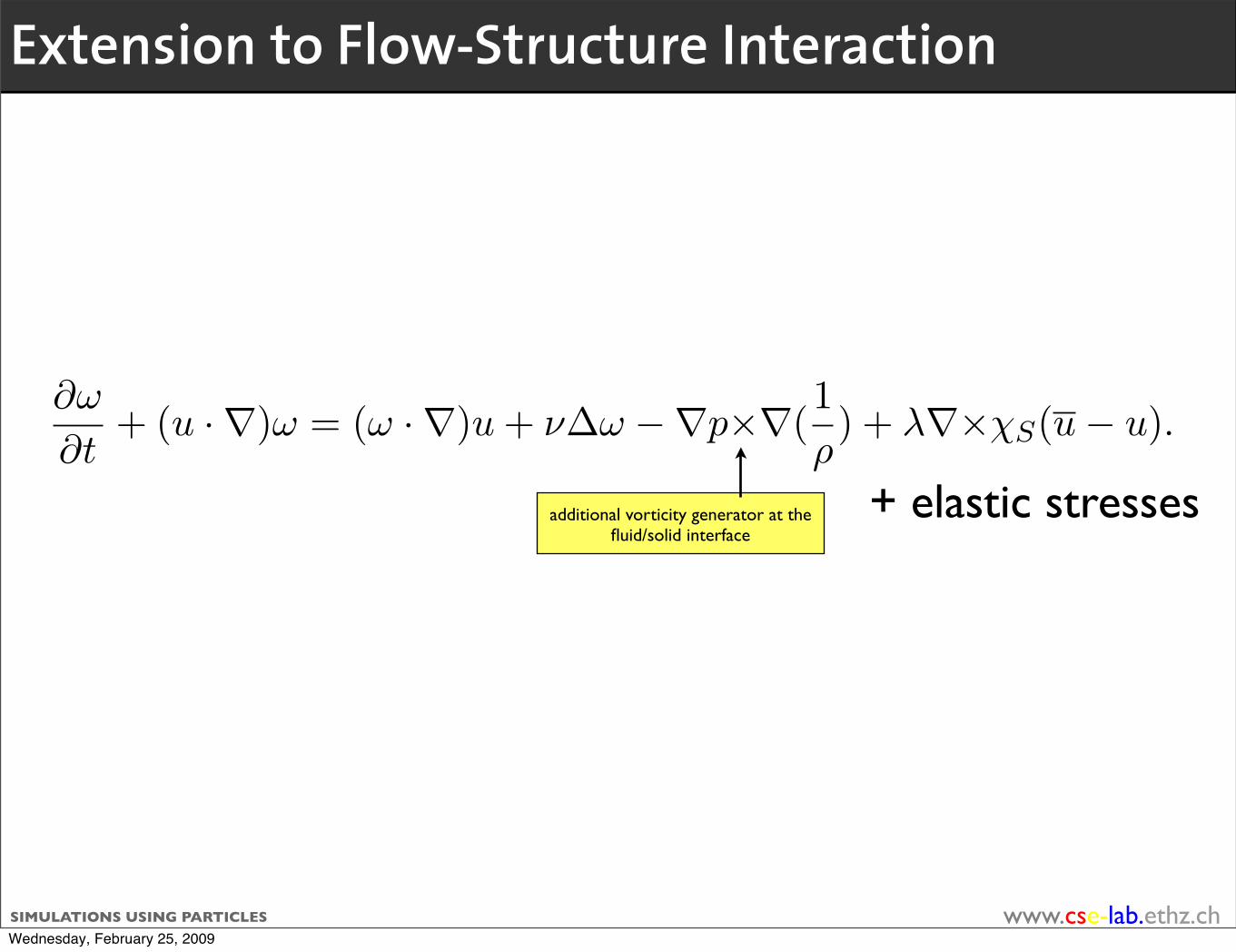
additional vorticity generator at the fluid/solid interface
+ elastic stresses
Extension to Flow-Structure Interaction
Wednesday, February 25, 2009

25 years DINFKwww.cse-lab.ethz.chSIMULATIONS USING PARTICLES
•fluid-solid system considered as a variable-density flow
58
Obstacle
Fluid
Tagged grid points for
the solution
of the linear system
Physical boundaryNumerical
boundary
Figure 35: Immersed boundary
6.2.3 IMMERSED BOUNDARY TECHNIQUES - THE PENALIZATION METHOD Theidea behind penalization method is to view obstacles, walls, etc .. as porous mediawhich absorb the velocity in a small layer on the boundary of the obstacle [2]. From amathematical point of view, it means assuming a flow everywhere, including inside theobstacles, and adding a term in the flow equation which drives the velocity back to zero- or whatever value is sought - inside the obstacles.
To be more specific, we consider, in a computational domain K, the case of an incom-pressible flow around an object S with prescribed velocity u inside S. We denote by λa penalization parameter, λ >> 1, and denote by χS the characteristic function of S (1inside, 0 outside). The model equation is then the following :
ρ
(∂u
∂t+ (u ·∇)u
)− ν∆u +∇p = ρ g + λ ρχS(u− u)forx ∈ K (92)
coupled with the incompressibility condition
div u = 0 for x ∈ K (93)
In the above equation ρ denotes the density, with value ρS in S and ρF in the fluidoutside S, F = K − S. If we want to use vortex particles to handle this penalizationmodel, we first need to derive the vorticity form of (92). Taking the curl of (92) we get
∂ω
∂t+ (u ·∇)ω = (ω ·∇)u + ν∆ω −∇p×∇(
1ρ) + λ∇×χS(u− u). (94)
This system has to be complemented by the usual system giving the velocity in terms ofthe vorticity :
∇ · u = 0inK;∇×u = ω inK. (95)
The right hand side above exhibits two terms : a so-called barotropic term, resultingfrom the density variations, already seen in variable density and free surface flows, and
additional vorticity generator at the fluid/solid interface
+ elastic stresses
Extension to Flow-Structure Interaction
Wednesday, February 25, 2009

25 years DINFKwww.cse-lab.ethz.chSIMULATIONS USING PARTICLES
•fluid-solid system considered as a variable-density flow•body velocity results from flow forces
58
Obstacle
Fluid
Tagged grid points for
the solution
of the linear system
Physical boundaryNumerical
boundary
Figure 35: Immersed boundary
6.2.3 IMMERSED BOUNDARY TECHNIQUES - THE PENALIZATION METHOD Theidea behind penalization method is to view obstacles, walls, etc .. as porous mediawhich absorb the velocity in a small layer on the boundary of the obstacle [2]. From amathematical point of view, it means assuming a flow everywhere, including inside theobstacles, and adding a term in the flow equation which drives the velocity back to zero- or whatever value is sought - inside the obstacles.
To be more specific, we consider, in a computational domain K, the case of an incom-pressible flow around an object S with prescribed velocity u inside S. We denote by λa penalization parameter, λ >> 1, and denote by χS the characteristic function of S (1inside, 0 outside). The model equation is then the following :
ρ
(∂u
∂t+ (u ·∇)u
)− ν∆u +∇p = ρ g + λ ρχS(u− u)forx ∈ K (92)
coupled with the incompressibility condition
div u = 0 for x ∈ K (93)
In the above equation ρ denotes the density, with value ρS in S and ρF in the fluidoutside S, F = K − S. If we want to use vortex particles to handle this penalizationmodel, we first need to derive the vorticity form of (92). Taking the curl of (92) we get
∂ω
∂t+ (u ·∇)ω = (ω ·∇)u + ν∆ω −∇p×∇(
1ρ) + λ∇×χS(u− u). (94)
This system has to be complemented by the usual system giving the velocity in terms ofthe vorticity :
∇ · u = 0inK;∇×u = ω inK. (95)
The right hand side above exhibits two terms : a so-called barotropic term, resultingfrom the density variations, already seen in variable density and free surface flows, and
additional vorticity generator at the fluid/solid interface
+ elastic stresses
Extension to Flow-Structure Interaction
Wednesday, February 25, 2009

25 years DINFKwww.cse-lab.ethz.chSIMULATIONS USING PARTICLES
•fluid-solid system considered as a variable-density flow•body velocity results from flow forces•velocity continuity obtained by penalization
58
Obstacle
Fluid
Tagged grid points for
the solution
of the linear system
Physical boundaryNumerical
boundary
Figure 35: Immersed boundary
6.2.3 IMMERSED BOUNDARY TECHNIQUES - THE PENALIZATION METHOD Theidea behind penalization method is to view obstacles, walls, etc .. as porous mediawhich absorb the velocity in a small layer on the boundary of the obstacle [2]. From amathematical point of view, it means assuming a flow everywhere, including inside theobstacles, and adding a term in the flow equation which drives the velocity back to zero- or whatever value is sought - inside the obstacles.
To be more specific, we consider, in a computational domain K, the case of an incom-pressible flow around an object S with prescribed velocity u inside S. We denote by λa penalization parameter, λ >> 1, and denote by χS the characteristic function of S (1inside, 0 outside). The model equation is then the following :
ρ
(∂u
∂t+ (u ·∇)u
)− ν∆u +∇p = ρ g + λ ρχS(u− u)forx ∈ K (92)
coupled with the incompressibility condition
div u = 0 for x ∈ K (93)
In the above equation ρ denotes the density, with value ρS in S and ρF in the fluidoutside S, F = K − S. If we want to use vortex particles to handle this penalizationmodel, we first need to derive the vorticity form of (92). Taking the curl of (92) we get
∂ω
∂t+ (u ·∇)ω = (ω ·∇)u + ν∆ω −∇p×∇(
1ρ) + λ∇×χS(u− u). (94)
This system has to be complemented by the usual system giving the velocity in terms ofthe vorticity :
∇ · u = 0inK;∇×u = ω inK. (95)
The right hand side above exhibits two terms : a so-called barotropic term, resultingfrom the density variations, already seen in variable density and free surface flows, and
additional vorticity generator at the fluid/solid interface
+ elastic stresses
Extension to Flow-Structure Interaction
Wednesday, February 25, 2009

25 years DINFKwww.cse-lab.ethz.chSIMULATIONS USING PARTICLES
•fluid-solid system considered as a variable-density flow•body velocity results from flow forces•velocity continuity obtained by penalization•contact between solid and/or elastic behavior through a level set model
58
Obstacle
Fluid
Tagged grid points for
the solution
of the linear system
Physical boundaryNumerical
boundary
Figure 35: Immersed boundary
6.2.3 IMMERSED BOUNDARY TECHNIQUES - THE PENALIZATION METHOD Theidea behind penalization method is to view obstacles, walls, etc .. as porous mediawhich absorb the velocity in a small layer on the boundary of the obstacle [2]. From amathematical point of view, it means assuming a flow everywhere, including inside theobstacles, and adding a term in the flow equation which drives the velocity back to zero- or whatever value is sought - inside the obstacles.
To be more specific, we consider, in a computational domain K, the case of an incom-pressible flow around an object S with prescribed velocity u inside S. We denote by λa penalization parameter, λ >> 1, and denote by χS the characteristic function of S (1inside, 0 outside). The model equation is then the following :
ρ
(∂u
∂t+ (u ·∇)u
)− ν∆u +∇p = ρ g + λ ρχS(u− u)forx ∈ K (92)
coupled with the incompressibility condition
div u = 0 for x ∈ K (93)
In the above equation ρ denotes the density, with value ρS in S and ρF in the fluidoutside S, F = K − S. If we want to use vortex particles to handle this penalizationmodel, we first need to derive the vorticity form of (92). Taking the curl of (92) we get
∂ω
∂t+ (u ·∇)ω = (ω ·∇)u + ν∆ω −∇p×∇(
1ρ) + λ∇×χS(u− u). (94)
This system has to be complemented by the usual system giving the velocity in terms ofthe vorticity :
∇ · u = 0inK;∇×u = ω inK. (95)
The right hand side above exhibits two terms : a so-called barotropic term, resultingfrom the density variations, already seen in variable density and free surface flows, and
additional vorticity generator at the fluid/solid interface
+ elastic stresses
NEED TO :
Extension to Flow-Structure Interaction
Wednesday, February 25, 2009

25 years DINFKwww.cse-lab.ethz.chSIMULATIONS USING PARTICLES
•fluid-solid system considered as a variable-density flow•body velocity results from flow forces•velocity continuity obtained by penalization•contact between solid and/or elastic behavior through a level set model
58
Obstacle
Fluid
Tagged grid points for
the solution
of the linear system
Physical boundaryNumerical
boundary
Figure 35: Immersed boundary
6.2.3 IMMERSED BOUNDARY TECHNIQUES - THE PENALIZATION METHOD Theidea behind penalization method is to view obstacles, walls, etc .. as porous mediawhich absorb the velocity in a small layer on the boundary of the obstacle [2]. From amathematical point of view, it means assuming a flow everywhere, including inside theobstacles, and adding a term in the flow equation which drives the velocity back to zero- or whatever value is sought - inside the obstacles.
To be more specific, we consider, in a computational domain K, the case of an incom-pressible flow around an object S with prescribed velocity u inside S. We denote by λa penalization parameter, λ >> 1, and denote by χS the characteristic function of S (1inside, 0 outside). The model equation is then the following :
ρ
(∂u
∂t+ (u ·∇)u
)− ν∆u +∇p = ρ g + λ ρχS(u− u)forx ∈ K (92)
coupled with the incompressibility condition
div u = 0 for x ∈ K (93)
In the above equation ρ denotes the density, with value ρS in S and ρF in the fluidoutside S, F = K − S. If we want to use vortex particles to handle this penalizationmodel, we first need to derive the vorticity form of (92). Taking the curl of (92) we get
∂ω
∂t+ (u ·∇)ω = (ω ·∇)u + ν∆ω −∇p×∇(
1ρ) + λ∇×χS(u− u). (94)
This system has to be complemented by the usual system giving the velocity in terms ofthe vorticity :
∇ · u = 0inK;∇×u = ω inK. (95)
The right hand side above exhibits two terms : a so-called barotropic term, resultingfrom the density variations, already seen in variable density and free surface flows, and
additional vorticity generator at the fluid/solid interface
+ elastic stresses
NEED TO : 1.compute pressure
Extension to Flow-Structure Interaction
Wednesday, February 25, 2009

25 years DINFKwww.cse-lab.ethz.chSIMULATIONS USING PARTICLES
•fluid-solid system considered as a variable-density flow•body velocity results from flow forces•velocity continuity obtained by penalization•contact between solid and/or elastic behavior through a level set model
58
Obstacle
Fluid
Tagged grid points for
the solution
of the linear system
Physical boundaryNumerical
boundary
Figure 35: Immersed boundary
6.2.3 IMMERSED BOUNDARY TECHNIQUES - THE PENALIZATION METHOD Theidea behind penalization method is to view obstacles, walls, etc .. as porous mediawhich absorb the velocity in a small layer on the boundary of the obstacle [2]. From amathematical point of view, it means assuming a flow everywhere, including inside theobstacles, and adding a term in the flow equation which drives the velocity back to zero- or whatever value is sought - inside the obstacles.
To be more specific, we consider, in a computational domain K, the case of an incom-pressible flow around an object S with prescribed velocity u inside S. We denote by λa penalization parameter, λ >> 1, and denote by χS the characteristic function of S (1inside, 0 outside). The model equation is then the following :
ρ
(∂u
∂t+ (u ·∇)u
)− ν∆u +∇p = ρ g + λ ρχS(u− u)forx ∈ K (92)
coupled with the incompressibility condition
div u = 0 for x ∈ K (93)
In the above equation ρ denotes the density, with value ρS in S and ρF in the fluidoutside S, F = K − S. If we want to use vortex particles to handle this penalizationmodel, we first need to derive the vorticity form of (92). Taking the curl of (92) we get
∂ω
∂t+ (u ·∇)ω = (ω ·∇)u + ν∆ω −∇p×∇(
1ρ) + λ∇×χS(u− u). (94)
This system has to be complemented by the usual system giving the velocity in terms ofthe vorticity :
∇ · u = 0inK;∇×u = ω inK. (95)
The right hand side above exhibits two terms : a so-called barotropic term, resultingfrom the density variations, already seen in variable density and free surface flows, and
additional vorticity generator at the fluid/solid interface
+ elastic stresses
NEED TO : 1.compute pressure2.compute solid velocity(ies)
Extension to Flow-Structure Interaction
Wednesday, February 25, 2009
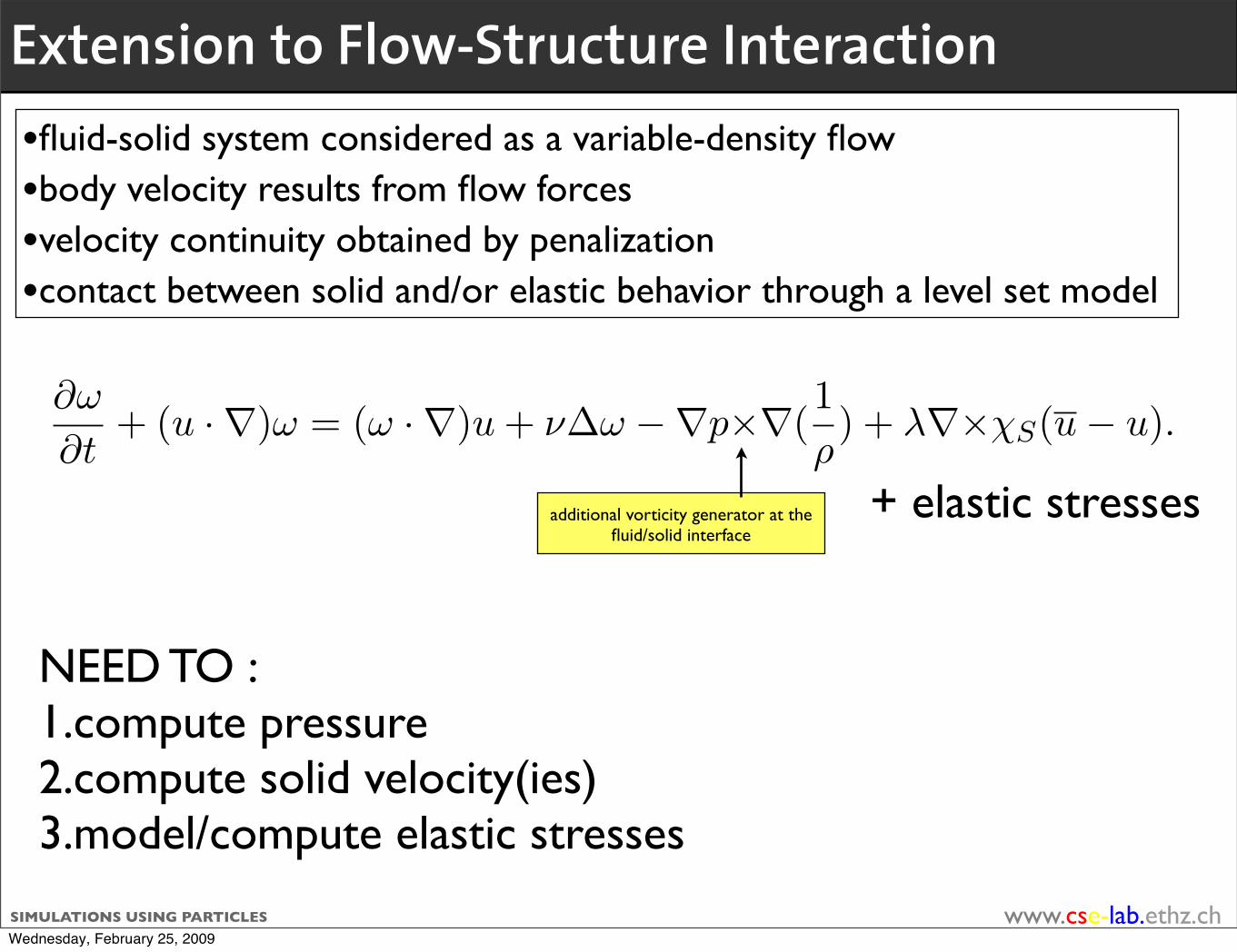
25 years DINFKwww.cse-lab.ethz.chSIMULATIONS USING PARTICLES
•fluid-solid system considered as a variable-density flow•body velocity results from flow forces•velocity continuity obtained by penalization•contact between solid and/or elastic behavior through a level set model
58
Obstacle
Fluid
Tagged grid points for
the solution
of the linear system
Physical boundaryNumerical
boundary
Figure 35: Immersed boundary
6.2.3 IMMERSED BOUNDARY TECHNIQUES - THE PENALIZATION METHOD Theidea behind penalization method is to view obstacles, walls, etc .. as porous mediawhich absorb the velocity in a small layer on the boundary of the obstacle [2]. From amathematical point of view, it means assuming a flow everywhere, including inside theobstacles, and adding a term in the flow equation which drives the velocity back to zero- or whatever value is sought - inside the obstacles.
To be more specific, we consider, in a computational domain K, the case of an incom-pressible flow around an object S with prescribed velocity u inside S. We denote by λa penalization parameter, λ >> 1, and denote by χS the characteristic function of S (1inside, 0 outside). The model equation is then the following :
ρ
(∂u
∂t+ (u ·∇)u
)− ν∆u +∇p = ρ g + λ ρχS(u− u)forx ∈ K (92)
coupled with the incompressibility condition
div u = 0 for x ∈ K (93)
In the above equation ρ denotes the density, with value ρS in S and ρF in the fluidoutside S, F = K − S. If we want to use vortex particles to handle this penalizationmodel, we first need to derive the vorticity form of (92). Taking the curl of (92) we get
∂ω
∂t+ (u ·∇)ω = (ω ·∇)u + ν∆ω −∇p×∇(
1ρ) + λ∇×χS(u− u). (94)
This system has to be complemented by the usual system giving the velocity in terms ofthe vorticity :
∇ · u = 0inK;∇×u = ω inK. (95)
The right hand side above exhibits two terms : a so-called barotropic term, resultingfrom the density variations, already seen in variable density and free surface flows, and
additional vorticity generator at the fluid/solid interface
+ elastic stresses
NEED TO : 1.compute pressure2.compute solid velocity(ies)3.model/compute elastic stresses
Extension to Flow-Structure Interaction
Wednesday, February 25, 2009

25 years DINFKwww.cse-lab.ethz.chSIMULATIONS USING PARTICLES
In an hybrid particle-grid method, the simplest is to go back to the velocity-pressure formulation :
58
Obstacle
Fluid
Tagged grid points for
the solution
of the linear system
Physical boundaryNumerical
boundary
Figure 35: Immersed boundary
6.2.3 IMMERSED BOUNDARY TECHNIQUES - THE PENALIZATION METHOD Theidea behind penalization method is to view obstacles, walls, etc .. as porous mediawhich absorb the velocity in a small layer on the boundary of the obstacle [2]. From amathematical point of view, it means assuming a flow everywhere, including inside theobstacles, and adding a term in the flow equation which drives the velocity back to zero- or whatever value is sought - inside the obstacles.
To be more specific, we consider, in a computational domain K, the case of an incom-pressible flow around an object S with prescribed velocity u inside S. We denote by λa penalization parameter, λ >> 1, and denote by χS the characteristic function of S (1inside, 0 outside). The model equation is then the following :
ρ
(∂u
∂t+ (u ·∇)u
)− ν∆u +∇p = ρ g + λ ρχS(u− u)forx ∈ K (92)
coupled with the incompressibility condition
div u = 0 for x ∈ K (93)
In the above equation ρ denotes the density, with value ρS in S and ρF in the fluidoutside S, F = K − S. If we want to use vortex particles to handle this penalizationmodel, we first need to derive the vorticity form of (92). Taking the curl of (92) we get
∂ω
∂t+ (u ·∇)ω = (ω ·∇)u + ν∆ω −∇p×∇(
1ρ) + λ∇×χS(u− u). (94)
This system has to be complemented by the usual system giving the velocity in terms ofthe vorticity :
∇ · u = 0inK;∇×u = ω inK. (95)
The right hand side above exhibits two terms : a so-called barotropic term, resultingfrom the density variations, already seen in variable density and free surface flows, and
⇒∇p in terms of u and its derivatives.
Evaluated by finite differences on the underlying grid form velocity values at the beginning of the step and at previous time-step
Pressure in a Vorticity Formulation ?Several possible ways in a vorticity formulation
Wednesday, February 25, 2009

25 years DINFKwww.cse-lab.ethz.chSIMULATIONS USING PARTICLES
Projection of flow velocity onto rigid body velocity:
60
tion term based on this level set. The level set equation is classically :
∂φS
∂t+ (u ·∇)φS = 0. (97)
The level set function is initialized as a distance function to the initial boundary of thesolid, positive inside and negative outside. The expression of the rigid motion u is actu-ally rather simple : it is obtained by averaging the velocity (to obtain the translation partof the rigid body - and the vorticity (to obtain the rotation) inside the body :
u =1
|S|
∫
KχSu dx +
(J−1
∫
KχSu× (x− xG) dx
)×(x− xG). (98)
We have denoted by χS the characteristic function of the solid which can be immediatelyrecovered from the level set function : χS(x) = (1 + sign(φS(x)))/2. The appealing
Figure 36: Kissing and tumbling of 2 spheres by a vortex level set method.
character of is model is the fact that it both relies on clear-cut numerical recipes (onecan actually prove that it converges, when numerical discretization parameters tend to0, to the exact physical solution) and is very easily implemented in a remeshed particlealgorithm. Such an algorithm will combines the following steps, for each time interval :
∂ω
∂t+ (u ·∇) ω = (ω ·∇)u + ν∆ω (99)
where J is the inertia matrix of the body K, and xG is its mass center.
Solid Velocities
Wednesday, February 25, 2009

25 years DINFKwww.cse-lab.ethz.chSIMULATIONS USING PARTICLES
Projection of flow velocity onto rigid body velocity:
60
tion term based on this level set. The level set equation is classically :
∂φS
∂t+ (u ·∇)φS = 0. (97)
The level set function is initialized as a distance function to the initial boundary of thesolid, positive inside and negative outside. The expression of the rigid motion u is actu-ally rather simple : it is obtained by averaging the velocity (to obtain the translation partof the rigid body - and the vorticity (to obtain the rotation) inside the body :
u =1
|S|
∫
KχSu dx +
(J−1
∫
KχSu× (x− xG) dx
)×(x− xG). (98)
We have denoted by χS the characteristic function of the solid which can be immediatelyrecovered from the level set function : χS(x) = (1 + sign(φS(x)))/2. The appealing
Figure 36: Kissing and tumbling of 2 spheres by a vortex level set method.
character of is model is the fact that it both relies on clear-cut numerical recipes (onecan actually prove that it converges, when numerical discretization parameters tend to0, to the exact physical solution) and is very easily implemented in a remeshed particlealgorithm. Such an algorithm will combines the following steps, for each time interval :
∂ω
∂t+ (u ·∇) ω = (ω ·∇)u + ν∆ω (99)
where J is the inertia matrix of the body K, and xG is its mass center.
average translation velocity average vorticity
E =1
ε
∫
E(|∇φ|)ζ(φ
ε) dx
T(γ(s, t), t) = λ(‖γs(s, t)‖ − 1)
−div(F (ψ, ∇ψ)∇ψ ⊗∇ψ)
(ut + (u · ∇)u) − div σ(ψ,Du,X, ∇X) + ∇p = 0
σ(ψ,Du,X, ∇X) = σS(X, ∇Xt∇X) + H(ψ/ε)
(
σF (Du) − σS(X, ∇Xt∇X)
)
ut + (u · ∇)u − ν∆u + ∇p = λ(u − u)χS
ωt + (u · ∇)ω = (ω · ∇)u + ν∆ω + λ(ω − ω)χS + λ(u − u) × n δ∂S
ωt + (u · ∇)ω = (ω · ∇)u + ν∆ω + (ω − ω)H(ϕ/ε) − (u − u) × ∇ϕ ζε(ϕ)
α4 = γ(Z)
∂φ
∂t+ (u · ∇)φ = 0
ρ
(
∂u
∂t+ (u · ∇)u
)
+ ∇p − ν∆u = f(φ, ∇φ)
ρ
(
∂u
∂t+ (u · ∇)u
)
+ ∇p = ν∆u + ρg + λχS(u − u) + γFe
λ >> 1 , γ = 0
Xt = u(X(r, s, t), t) =
∫
u(x, t)δ(x − X(r, s, t)) dx
f(x, t) =
∫
F(r, s, t)δ(x − X(r, s, t) drds
τ =V
4
3π
(
A4π
)3/2∈ [0, 1]
4
•K is captured by a level set function, advected with the rigid motion ū :
Solid Velocities
Wednesday, February 25, 2009

25 years DINFKwww.cse-lab.ethz.chSIMULATIONS USING PARTICLES
Projection of flow velocity onto rigid body velocity:
60
tion term based on this level set. The level set equation is classically :
∂φS
∂t+ (u ·∇)φS = 0. (97)
The level set function is initialized as a distance function to the initial boundary of thesolid, positive inside and negative outside. The expression of the rigid motion u is actu-ally rather simple : it is obtained by averaging the velocity (to obtain the translation partof the rigid body - and the vorticity (to obtain the rotation) inside the body :
u =1
|S|
∫
KχSu dx +
(J−1
∫
KχSu× (x− xG) dx
)×(x− xG). (98)
We have denoted by χS the characteristic function of the solid which can be immediatelyrecovered from the level set function : χS(x) = (1 + sign(φS(x)))/2. The appealing
Figure 36: Kissing and tumbling of 2 spheres by a vortex level set method.
character of is model is the fact that it both relies on clear-cut numerical recipes (onecan actually prove that it converges, when numerical discretization parameters tend to0, to the exact physical solution) and is very easily implemented in a remeshed particlealgorithm. Such an algorithm will combines the following steps, for each time interval :
∂ω
∂t+ (u ·∇) ω = (ω ·∇)u + ν∆ω (99)
where J is the inertia matrix of the body K, and xG is its mass center.
•Accumulating rigid motions step by step allows to advect exactly K from its inital stage (the advection equation is not solved - Prevents numerical errors to slightly deform K)
average translation velocity average vorticity
E =1
ε
∫
E(|∇φ|)ζ(φ
ε) dx
T(γ(s, t), t) = λ(‖γs(s, t)‖ − 1)
−div(F (ψ, ∇ψ)∇ψ ⊗∇ψ)
(ut + (u · ∇)u) − div σ(ψ,Du,X, ∇X) + ∇p = 0
σ(ψ,Du,X, ∇X) = σS(X, ∇Xt∇X) + H(ψ/ε)
(
σF (Du) − σS(X, ∇Xt∇X)
)
ut + (u · ∇)u − ν∆u + ∇p = λ(u − u)χS
ωt + (u · ∇)ω = (ω · ∇)u + ν∆ω + λ(ω − ω)χS + λ(u − u) × n δ∂S
ωt + (u · ∇)ω = (ω · ∇)u + ν∆ω + (ω − ω)H(ϕ/ε) − (u − u) × ∇ϕ ζε(ϕ)
α4 = γ(Z)
∂φ
∂t+ (u · ∇)φ = 0
ρ
(
∂u
∂t+ (u · ∇)u
)
+ ∇p − ν∆u = f(φ, ∇φ)
ρ
(
∂u
∂t+ (u · ∇)u
)
+ ∇p = ν∆u + ρg + λχS(u − u) + γFe
λ >> 1 , γ = 0
Xt = u(X(r, s, t), t) =
∫
u(x, t)δ(x − X(r, s, t)) dx
f(x, t) =
∫
F(r, s, t)δ(x − X(r, s, t) drds
τ =V
4
3π
(
A4π
)3/2∈ [0, 1]
4
•K is captured by a level set function, advected with the rigid motion ū :
Solid Velocities
Wednesday, February 25, 2009

25 years DINFKwww.cse-lab.ethz.chSIMULATIONS USING PARTICLES
contact/collision model based on dynamical repulsive model, distributed on the skin of the bodies through a level set technique
only result from viscous dissipation in the boundary layer. Here we consider a direct approach that will beagain rely on interface capturing by means of level set functions. Using level set functions to deal with colli-sions is actually not new. These techniques were proposed under the names of implicit surfaces in physicalmodeling for the animation of elastic or rigid bodies (see for instance [4]). In these methods, body surfacesare captured by implicit surfaces which are used to detect penetration. Distance functions serve to computethe amount of overlapping. This information is used to derive forces on the surfaces that are subsequentlypropagated throughout the bodies in some ad hoc fashion in order to remove this overlapping. Our methoddiffers from these implicit surfaces techniques in particular in that we compute a single force which is essen-tially parameter free and simply supplements the flow equation. The level set collision formulation is only away to distribute in a clear-cut way repulsive point forces over the surface of the bodies.
2.2.1. One-dimensional modelLike in [14], we start from a dynamical system for the one-dimensional collision of a material point located
at xðtÞ > 0 with a wall assumed to be located at x ¼ 0. We choose a dynamical system which is both shortrange and singular at the contact point. This dynamical system reads
€x ¼ jxexpð$x=!Þ; ð20Þ
where j is a coefficient which has the dimension of the square of a velocity. It is an Hamiltonian model actingon a width of the order of ! around x ¼ 0. As a result, it produces an energy preserving collision at a distanceOð!Þ of the wall. More precisely, its potential energy is, up to an additive constant, given by
EðxÞ ¼Z x
1
jsexpð$s=!Þ; ds ¼
Z x=!
1=!
jyexpð$yÞdy:
Consider a point initially located at xð0Þ ¼ 1 and with velocity vð0Þ ¼ v0 < 0. If we denote by xH its minimallocation (a point at which the velocity is zero), by conservation of energy we have
xH ¼ !G!ðv20=2jÞ ’ !Gðv20=2jÞ for ! % 1; ð21Þ
where G! and G denote the inverse functions respectively of the functions F ! and F defined as
F !ðxÞ ¼Z 1=!
x
1
yexpð$yÞdy; F ðxÞ ¼
Z þ1
x
1
yexpð$yÞdy:
Eq. (21) states that the rebound width scales as !.
2.2.2. Level set modelThe level set formulation allows to translate the simple dynamical system above into a body force distrib-
uted on the surface. Level set functions indeed give simultaneously access to distances, normals and surfaceintegrals on the interfaces. If the rigid bodies are labelled by indices i, to compute the rebound of Si andSj, imbedded in a fluid with fluid interfaces respectively captured by level set functions /i and /j, point forcessimilar to the right hand side of (20) are implemented on each point of the interface of Si, localized through thelevel set function /i. The direction of the force and the distance of the boundary points of Si to the body Sj areobtained directly from the level set function /j. From these observations, one readily obtains the followingforce resulting from all possible body interactions:
fcolðxÞ ¼ $qX
ij
jij
!f
/iðxÞ!
! "$/jðxÞ/jðxÞ
expð$/jðxÞ=!Þ: ð22Þ
The minus sign above comes from the fact that, by the definition of the level set functions, $/j is orientedinwards with respect to the body Sj. The function f in the above expression is a one-dimensional cut-off func-tion. In view of (21), the coefficients jij are to be chosen proportional to the square of the relative velocities ofthe corresponding bodies just before the collision. Note that in the above equation, we have used the fact al-ready mentioned that since the body/fluid interface level set functions are transported by rigid body velocity,
6 M. Coquerelle, G.-H. Cottet / Journal of Computational Physics xxx (2008) xxx–xxx
ARTICLE IN PRESS
Please cite this article in press as: M. Coquerelle, G.-H. Cottet, A vortex level set method for the two-way coupling ..., J.Comput. Phys. (2008), doi:10.1016/j.jcp.2008.03.041
1D dynamical system for a collision on a range O(v2/κ)
only result from viscous dissipation in the boundary layer. Here we consider a direct approach that will beagain rely on interface capturing by means of level set functions. Using level set functions to deal with colli-sions is actually not new. These techniques were proposed under the names of implicit surfaces in physicalmodeling for the animation of elastic or rigid bodies (see for instance [4]). In these methods, body surfacesare captured by implicit surfaces which are used to detect penetration. Distance functions serve to computethe amount of overlapping. This information is used to derive forces on the surfaces that are subsequentlypropagated throughout the bodies in some ad hoc fashion in order to remove this overlapping. Our methoddiffers from these implicit surfaces techniques in particular in that we compute a single force which is essen-tially parameter free and simply supplements the flow equation. The level set collision formulation is only away to distribute in a clear-cut way repulsive point forces over the surface of the bodies.
2.2.1. One-dimensional modelLike in [14], we start from a dynamical system for the one-dimensional collision of a material point located
at xðtÞ > 0 with a wall assumed to be located at x ¼ 0. We choose a dynamical system which is both shortrange and singular at the contact point. This dynamical system reads
€x ¼ jxexpð$x=!Þ; ð20Þ
where j is a coefficient which has the dimension of the square of a velocity. It is an Hamiltonian model actingon a width of the order of ! around x ¼ 0. As a result, it produces an energy preserving collision at a distanceOð!Þ of the wall. More precisely, its potential energy is, up to an additive constant, given by
EðxÞ ¼Z x
1
jsexpð$s=!Þ; ds ¼
Z x=!
1=!
jyexpð$yÞdy:
Consider a point initially located at xð0Þ ¼ 1 and with velocity vð0Þ ¼ v0 < 0. If we denote by xH its minimallocation (a point at which the velocity is zero), by conservation of energy we have
xH ¼ !G!ðv20=2jÞ ’ !Gðv20=2jÞ for ! % 1; ð21Þ
where G! and G denote the inverse functions respectively of the functions F ! and F defined as
F !ðxÞ ¼Z 1=!
x
1
yexpð$yÞdy; F ðxÞ ¼
Z þ1
x
1
yexpð$yÞdy:
Eq. (21) states that the rebound width scales as !.
2.2.2. Level set modelThe level set formulation allows to translate the simple dynamical system above into a body force distrib-
uted on the surface. Level set functions indeed give simultaneously access to distances, normals and surfaceintegrals on the interfaces. If the rigid bodies are labelled by indices i, to compute the rebound of Si andSj, imbedded in a fluid with fluid interfaces respectively captured by level set functions /i and /j, point forcessimilar to the right hand side of (20) are implemented on each point of the interface of Si, localized through thelevel set function /i. The direction of the force and the distance of the boundary points of Si to the body Sj areobtained directly from the level set function /j. From these observations, one readily obtains the followingforce resulting from all possible body interactions:
fcolðxÞ ¼ $qX
ij
jij
!f
/iðxÞ!
! "$/jðxÞ/jðxÞ
expð$/jðxÞ=!Þ: ð22Þ
The minus sign above comes from the fact that, by the definition of the level set functions, $/j is orientedinwards with respect to the body Sj. The function f in the above expression is a one-dimensional cut-off func-tion. In view of (21), the coefficients jij are to be chosen proportional to the square of the relative velocities ofthe corresponding bodies just before the collision. Note that in the above equation, we have used the fact al-ready mentioned that since the body/fluid interface level set functions are transported by rigid body velocity,
6 M. Coquerelle, G.-H. Cottet / Journal of Computational Physics xxx (2008) xxx–xxx
ARTICLE IN PRESS
Please cite this article in press as: M. Coquerelle, G.-H. Cottet, A vortex level set method for the two-way coupling ..., J.Comput. Phys. (2008), doi:10.1016/j.jcp.2008.03.041
translation into an interface-distributed contact force:
Solid body Collisions
Wednesday, February 25, 2009

25 years DINFKwww.cse-lab.ethz.chSIMULATIONS USING PARTICLES
A hybrid particle-grid method for flows interacting with rigid bodies - [Coquerelle-Cottet 2008]
Wednesday, February 25, 2009

25 years DINFKwww.cse-lab.ethz.chSIMULATIONS USING PARTICLES
time 0: initialize flow and assign level set signed-distance ū functions to each body
A hybrid particle-grid method for flows interacting with rigid bodies - [Coquerelle-Cottet 2008]
Wednesday, February 25, 2009

25 years DINFKwww.cse-lab.ethz.chSIMULATIONS USING PARTICLES
time 0: initialize flow and assign level set signed-distance ū functions to each body
step iterations (black on grid, red on particles):
A hybrid particle-grid method for flows interacting with rigid bodies - [Coquerelle-Cottet 2008]
Wednesday, February 25, 2009
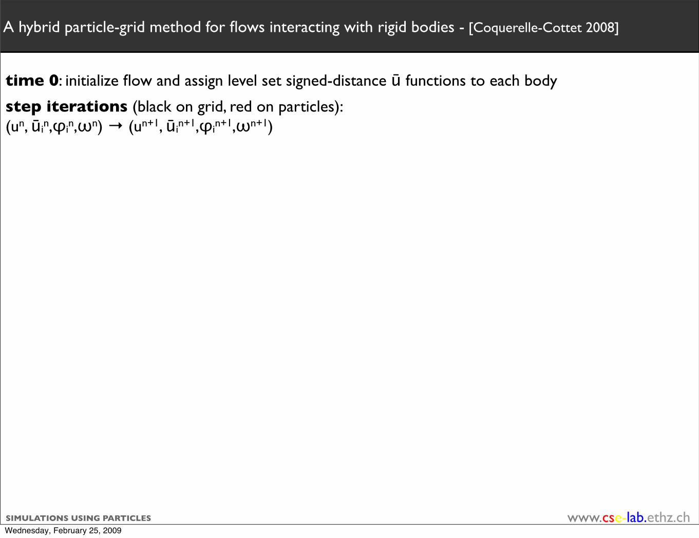
25 years DINFKwww.cse-lab.ethz.chSIMULATIONS USING PARTICLES
time 0: initialize flow and assign level set signed-distance ū functions to each body
step iterations (black on grid, red on particles): (un, ūin,φin,ωn) → (un+1, ūin+1,φin+1,ωn+1)
•advance exactly each level set function φin with the corresponding rigid motion ūin : → φin+1
•compute collision forces
A hybrid particle-grid method for flows interacting with rigid bodies - [Coquerelle-Cottet 2008]
Wednesday, February 25, 2009

25 years DINFKwww.cse-lab.ethz.chSIMULATIONS USING PARTICLES
time 0: initialize flow and assign level set signed-distance ū functions to each body
step iterations (black on grid, red on particles): (un, ūin,φin,ωn) → (un+1, ūin+1,φin+1,ωn+1)
•advance exactly each level set function φin with the corresponding rigid motion ūin : → φin+1
only result from viscous dissipation in the boundary layer. Here we consider a direct approach that will beagain rely on interface capturing by means of level set functions. Using level set functions to deal with colli-sions is actually not new. These techniques were proposed under the names of implicit surfaces in physicalmodeling for the animation of elastic or rigid bodies (see for instance [4]). In these methods, body surfacesare captured by implicit surfaces which are used to detect penetration. Distance functions serve to computethe amount of overlapping. This information is used to derive forces on the surfaces that are subsequentlypropagated throughout the bodies in some ad hoc fashion in order to remove this overlapping. Our methoddiffers from these implicit surfaces techniques in particular in that we compute a single force which is essen-tially parameter free and simply supplements the flow equation. The level set collision formulation is only away to distribute in a clear-cut way repulsive point forces over the surface of the bodies.
2.2.1. One-dimensional modelLike in [14], we start from a dynamical system for the one-dimensional collision of a material point located
at xðtÞ > 0 with a wall assumed to be located at x ¼ 0. We choose a dynamical system which is both shortrange and singular at the contact point. This dynamical system reads
€x ¼ jxexpð$x=!Þ; ð20Þ
where j is a coefficient which has the dimension of the square of a velocity. It is an Hamiltonian model actingon a width of the order of ! around x ¼ 0. As a result, it produces an energy preserving collision at a distanceOð!Þ of the wall. More precisely, its potential energy is, up to an additive constant, given by
EðxÞ ¼Z x
1
jsexpð$s=!Þ; ds ¼
Z x=!
1=!
jyexpð$yÞdy:
Consider a point initially located at xð0Þ ¼ 1 and with velocity vð0Þ ¼ v0 < 0. If we denote by xH its minimallocation (a point at which the velocity is zero), by conservation of energy we have
xH ¼ !G!ðv20=2jÞ ’ !Gðv20=2jÞ for ! % 1; ð21Þ
where G! and G denote the inverse functions respectively of the functions F ! and F defined as
F !ðxÞ ¼Z 1=!
x
1
yexpð$yÞdy; F ðxÞ ¼
Z þ1
x
1
yexpð$yÞdy:
Eq. (21) states that the rebound width scales as !.
2.2.2. Level set modelThe level set formulation allows to translate the simple dynamical system above into a body force distrib-
uted on the surface. Level set functions indeed give simultaneously access to distances, normals and surfaceintegrals on the interfaces. If the rigid bodies are labelled by indices i, to compute the rebound of Si andSj, imbedded in a fluid with fluid interfaces respectively captured by level set functions /i and /j, point forcessimilar to the right hand side of (20) are implemented on each point of the interface of Si, localized through thelevel set function /i. The direction of the force and the distance of the boundary points of Si to the body Sj areobtained directly from the level set function /j. From these observations, one readily obtains the followingforce resulting from all possible body interactions:
fcolðxÞ ¼ $qX
ij
jij
!f
/iðxÞ!
! "$/jðxÞ/jðxÞ
expð$/jðxÞ=!Þ: ð22Þ
The minus sign above comes from the fact that, by the definition of the level set functions, $/j is orientedinwards with respect to the body Sj. The function f in the above expression is a one-dimensional cut-off func-tion. In view of (21), the coefficients jij are to be chosen proportional to the square of the relative velocities ofthe corresponding bodies just before the collision. Note that in the above equation, we have used the fact al-ready mentioned that since the body/fluid interface level set functions are transported by rigid body velocity,
6 M. Coquerelle, G.-H. Cottet / Journal of Computational Physics xxx (2008) xxx–xxx
ARTICLE IN PRESS
Please cite this article in press as: M. Coquerelle, G.-H. Cottet, A vortex level set method for the two-way coupling ..., J.Comput. Phys. (2008), doi:10.1016/j.jcp.2008.03.041
•compute collision forces
A hybrid particle-grid method for flows interacting with rigid bodies - [Coquerelle-Cottet 2008]
Wednesday, February 25, 2009

25 years DINFKwww.cse-lab.ethz.chSIMULATIONS USING PARTICLES
time 0: initialize flow and assign level set signed-distance ū functions to each body
step iterations (black on grid, red on particles): (un, ūin,φin,ωn) → (un+1, ūin+1,φin+1,ωn+1)
•advance exactly each level set function φin with the corresponding rigid motion ūin : → φin+1
•compute collision forces
•update rigid body motions (no vorticity of collision force needed)
•update vorticity on the grid with
A hybrid particle-grid method for flows interacting with rigid bodies - [Coquerelle-Cottet 2008]
Wednesday, February 25, 2009
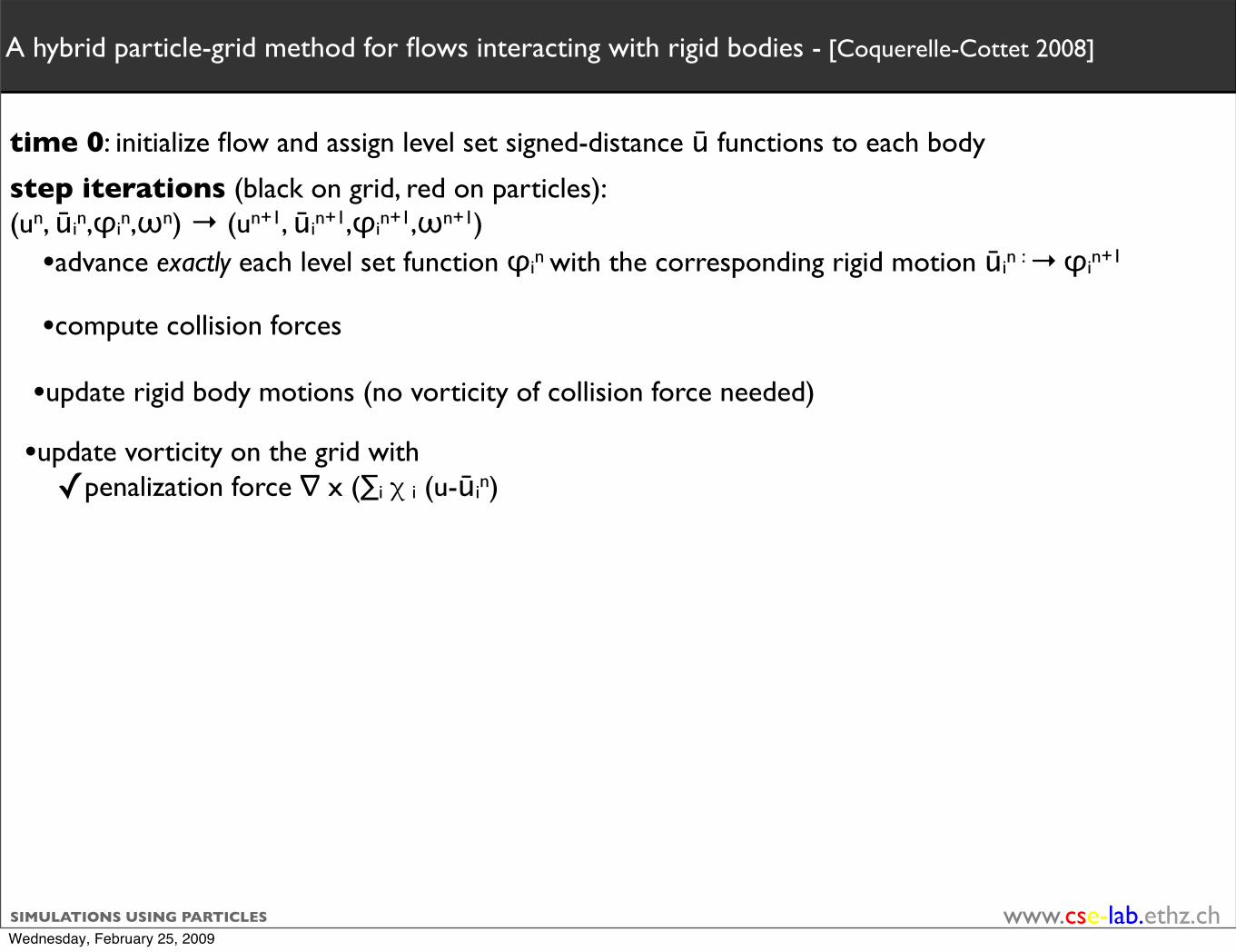
25 years DINFKwww.cse-lab.ethz.chSIMULATIONS USING PARTICLES
time 0: initialize flow and assign level set signed-distance ū functions to each body
step iterations (black on grid, red on particles): (un, ūin,φin,ωn) → (un+1, ūin+1,φin+1,ωn+1)
•advance exactly each level set function φin with the corresponding rigid motion ūin : → φin+1
•compute collision forces
•update rigid body motions (no vorticity of collision force needed)
•update vorticity on the grid withpenalization force ∇ x (∑iχi (u-ūin)
A hybrid particle-grid method for flows interacting with rigid bodies - [Coquerelle-Cottet 2008]
Wednesday, February 25, 2009

25 years DINFKwww.cse-lab.ethz.chSIMULATIONS USING PARTICLES
time 0: initialize flow and assign level set signed-distance ū functions to each body
step iterations (black on grid, red on particles): (un, ūin,φin,ωn) → (un+1, ūin+1,φin+1,ωn+1)
•advance exactly each level set function φin with the corresponding rigid motion ūin : → φin+1
•compute collision forces
•update rigid body motions (no vorticity of collision force needed)
•update vorticity on the grid withpenalization force ∇ x (∑iχi (u-ūin)pressure gradients
•push particles (transport-stretching-diffusion of vorticity)
10
Figure 5: Vortex Method simulations of solid particle ladden flows with two way cou-pling [97].
The vorticity field ω is related to the velocity field u by ω = ∇ × u. This equationtogether with the incompressiblity constraint
div u = 0 (19)
and suitable boundary conditions allows to express the velocity in terms of the vortic-ity (we will come back later to this important point). Equation (18) thus appears as anonlinear advection-diffusion equation for the vorticity. The diffusion term is just oneparticular instance of the right hand side F in (3). One particular and appealing featureof this form of the flow equations is that the divergence free constraint is not directlyinvolved in the transport equation. Also, the equation points straight to the very natureof vorticity dynamics in incompressible flows: transport and dissipation (in 2 and 3D), change of orientation and strengthening (in 3D only, since in 2D the term (ω ·∇) uvanishes). A vortex particle method consists of sampling vorticity on points that followthe flow field:
ω(x, t) =∑
p
ωpδ(x− xp) (20)
withdxp
dt= u(xp, t) (21)
dωp
dt= [∇u(xp, t)]ωp + ν ∆ω(xp). (22)
In the above equation [∇u(xp, t)] is the tensor made of all derivatives of the velocity. Theway to compute this term as well as the diffusion term remains to be specified. Vortex
A hybrid particle-grid method for flows interacting with rigid bodies - [Coquerelle-Cottet 2008]
Wednesday, February 25, 2009

25 years DINFKwww.cse-lab.ethz.chSIMULATIONS USING PARTICLES
time 0: initialize flow and assign level set signed-distance ū functions to each body
step iterations (black on grid, red on particles): (un, ūin,φin,ωn) → (un+1, ūin+1,φin+1,ωn+1)
•advance exactly each level set function φin with the corresponding rigid motion ūin : → φin+1
•compute collision forces
•update rigid body motions (no vorticity of collision force needed)
•update vorticity on the grid withpenalization force ∇ x (∑iχi (u-ūin)pressure gradients
•push particles (transport-stretching-diffusion of vorticity)
A hybrid particle-grid method for flows interacting with rigid bodies - [Coquerelle-Cottet 2008]
Wednesday, February 25, 2009
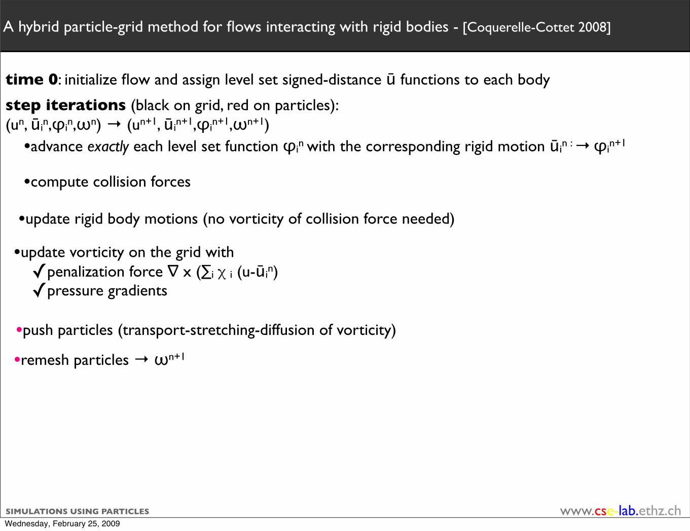
25 years DINFKwww.cse-lab.ethz.chSIMULATIONS USING PARTICLES
time 0: initialize flow and assign level set signed-distance ū functions to each body
step iterations (black on grid, red on particles): (un, ūin,φin,ωn) → (un+1, ūin+1,φin+1,ωn+1)
•advance exactly each level set function φin with the corresponding rigid motion ūin : → φin+1
•compute collision forces
•update rigid body motions (no vorticity of collision force needed)
•update vorticity on the grid withpenalization force ∇ x (∑iχi (u-ūin)pressure gradients
•push particles (transport-stretching-diffusion of vorticity)
•remesh particles → ωn+1
•compute flow velocity with a fast FFT-based Poisson solver → un+1
•compute rigid body motions
60
tion term based on this level set. The level set equation is classically :
∂φS
∂t+ (u ·∇)φS = 0. (97)
The level set function is initialized as a distance function to the initial boundary of thesolid, positive inside and negative outside. The expression of the rigid motion u is actu-ally rather simple : it is obtained by averaging the velocity (to obtain the translation partof the rigid body - and the vorticity (to obtain the rotation) inside the body :
u =1
|S|
∫
KχSu dx +
(J−1
∫
KχSu× (x− xG) dx
)×(x− xG). (98)
We have denoted by χS the characteristic function of the solid which can be immediatelyrecovered from the level set function : χS(x) = (1 + sign(φS(x)))/2. The appealing
Figure 36: Kissing and tumbling of 2 spheres by a vortex level set method.
character of is model is the fact that it both relies on clear-cut numerical recipes (onecan actually prove that it converges, when numerical discretization parameters tend to0, to the exact physical solution) and is very easily implemented in a remeshed particlealgorithm. Such an algorithm will combines the following steps, for each time interval :
∂ω
∂t+ (u ·∇) ω = (ω ·∇)u + ν∆ω (99)
A hybrid particle-grid method for flows interacting with rigid bodies - [Coquerelle-Cottet 2008]
Wednesday, February 25, 2009

25 years DINFKwww.cse-lab.ethz.chSIMULATIONS USING PARTICLES
time 0: initialize flow and assign level set signed-distance ū functions to each body
step iterations (black on grid, red on particles): (un, ūin,φin,ωn) → (un+1, ūin+1,φin+1,ωn+1)
•advance exactly each level set function φin with the corresponding rigid motion ūin : → φin+1
•compute collision forces
•update rigid body motions (no vorticity of collision force needed)
•update vorticity on the grid withpenalization force ∇ x (∑iχi (u-ūin)pressure gradients
•push particles (transport-stretching-diffusion of vorticity)
•remesh particles → ωn+1
•compute flow velocity with a fast FFT-based Poisson solver → un+1
•compute rigid body motions
A hybrid particle-grid method for flows interacting with rigid bodies - [Coquerelle-Cottet 2008]
Wednesday, February 25, 2009

25 years DINFKwww.cse-lab.ethz.chSIMULATIONS USING PARTICLES
SUMMARY
Final remaks: close to the projection method in [Sharma-Patankar 2005], but allows better fit of rigid body by implicit treatment on penalizationcan also add to collision force
•free surfaces, with or without surface tension, captured by additional level set functions•elastic fluid-structure interaction of the form F(φ,∇φ).
In these cases the level set equations must be solved (preferably with particles)
Wednesday, February 25, 2009

25 years DINFKwww.cse-lab.ethz.chSIMULATIONS USING PARTICLES
•on the GRID Poisson solver and finite-differences
SUMMARY
Final remaks: close to the projection method in [Sharma-Patankar 2005], but allows better fit of rigid body by implicit treatment on penalizationcan also add to collision force
•free surfaces, with or without surface tension, captured by additional level set functions•elastic fluid-structure interaction of the form F(φ,∇φ).
In these cases the level set equations must be solved (preferably with particles)
Wednesday, February 25, 2009

25 years DINFKwww.cse-lab.ethz.chSIMULATIONS USING PARTICLES
•on the GRID Poisson solver and finite-differences•on the PARTICLES : time-stepping of flow
most of the CPU time on remeshing
SUMMARY
Final remaks: close to the projection method in [Sharma-Patankar 2005], but allows better fit of rigid body by implicit treatment on penalizationcan also add to collision force
•free surfaces, with or without surface tension, captured by additional level set functions•elastic fluid-structure interaction of the form F(φ,∇φ).
In these cases the level set equations must be solved (preferably with particles)
Wednesday, February 25, 2009

25 years DINFKwww.cse-lab.ethz.chSIMULATIONS USING PARTICLES
•on the GRID Poisson solver and finite-differences•on the PARTICLES : time-stepping of flow
most of the CPU time on remeshinggain over grid-based methods through large time-steps and localization of computational effort (vorticity support) on interfaces.
SUMMARY
Final remaks: close to the projection method in [Sharma-Patankar 2005], but allows better fit of rigid body by implicit treatment on penalizationcan also add to collision force
•free surfaces, with or without surface tension, captured by additional level set functions•elastic fluid-structure interaction of the form F(φ,∇φ).
In these cases the level set equations must be solved (preferably with particles)
Wednesday, February 25, 2009