Border Security – Ground Teamaustin/enes489p/projects2011a/...Border Security – Ground Team 1...

Border Security – Ground Team

ENES 489P Spring 2011

Instructors: Dr. Mark Austin Dr. John Baras

Dr. Shah-An Yang

Ground Team Members: Jessica Jones

Matthew Marsh Aaron Olszewski

Senay Tekle Phil Tucci

Border Security – Ground Team 1

Abstract

We will develop a more efficient system to provide border security by focusing on surveillance and detection techniques. In order to do this we will split into two sub-groups - one group will be responsible for air surveillance and the other will be responsible for ground surveillance. The final goal is for both groups to come together to provide a comprehensive strategy for border security that will reduce the need for border security agent involvement on the front line. For the purpose of this study we will be focusing on the U.S. – Mexico border. The goal of the ground team is to detect, classify, and communicate unauthorized intrusions into the U.S. There are three possible ways to gain entry into the U.S. from the ground: using underground tunnels, travelling through the regions of the border without physical fences, and climbing over or cutting through the fence.

The ground team will design a multi-layered system consisting of both virtual and physical boundaries to guard against these methods of entry. The physical boundary will consist of the current fencing already in use by U.S. Customs and Border Protection (CBP), augmented by additional physical structures and communications centers. Previous efforts to incorporate sensor technology into the border security, such as Boeing’s SBInet, will also be integrated into our design to maximize efficiency and minimize cost. The virtual boundary will consist of multiple sensors networked to provide full ground coverage of areas that cannot be manually patrolled or bounded by a physical structure. The virtual border will use various types of sensors, including seismic sensors, thermal imaging, vibration detection, cameras etc. Sensor diversity will increase the probability of detecting intruders while minimizing false alarms due to inclement weather, large wildlife, and other natural occurrences. Most of the sensors in the virtual border will maintain a “low-power” state. Long range sensors, manned patrols, and aerial surveillance will provide the initial detection of an unauthorized incursion. At this point, mid-range and close range sensors will be brought into a fully powered state in order to track and further classify the incursion. The sensor network will provide real time and near-real time data to CBP agents in communications centers along the border. Once the incursion has been confirmed and classified as intruders, the closest CBP agents can respond in manned air or ground vehicles.

Figure 1: Image Source from http://www.wikipedia.org/


Table of Contents 1. Problem Statement .................................................................................................................. 4

1.1. Border Security ............................................................................................................... 4 1.2. Description of Border ..................................................................................................... 4 1.3. Possible Sensors.............................................................................................................. 4 1.4. Boeing’s SBInet .............................................................................................................. 5 1.5. Our Objectives ................................................................................................................ 6

2. Use Case Development ........................................................................................................... 7 2.1. Actors.............................................................................................................................. 7 2.2. Use Case 1 – Fence Search Case .................................................................................... 8 2.3. Use Case 2 – Fence Detection Case................................................................................ 9 2.4. Use Case 3 - Sector Ground Base Intelligence Gathering Case ................................... 11 2.5. Use Case 4 - Sector Ground Base Detection Case........................................................ 13 2.6. Use Case 5 - Headquarters Intelligence Gathering Case .............................................. 15 2.7. Use Case 6 - Headquarters Detection Case................................................................... 17 2.8. Use Case 7 - Fence External Failure Case .................................................................... 19 2.9. Use Case 8 - System Power Failure Case ..................................................................... 21 2.10. Use Case 9 - Border Patrol Agent Tracking Case..................................................... 23

3. Requirements Engineering.................................................................................................... 26 3.1. Requirements ................................................................................................................ 26 3.2. Traceability ................................................................................................................... 28

4. System-Level Design ............................................................................................................ 31 4.1. System Structure Diagrams........................................................................................... 31 4.2. System Level Diagram.................................................................................................. 32

5. Simplified Approach to Trade-off Analysis ......................................................................... 34 5.1. Trade-off Analysis ........................................................................................................ 34

6. General Conclusions ............................................................................................................. 45 Appendix....................................................................................................................................... 46 Bibliography ................................................................................................................................. 69 Sign-off Sheet ............................................................................................................................... 71


Table of Figures Figure 2: Relationship between Actors and Use Cases .................................................................. 7 Figure 3: Fence Search Case........................................................................................................... 8 Figure 4: Fence Search Case........................................................................................................... 9 Figure 5: Fence Detection Case .................................................................................................... 10 Figure 6: Fence Detection Case .................................................................................................... 11 Figure 7: Sector Ground Base Intelligence Gathering Case ......................................................... 12 Figure 8: Sector Ground Base Intelligence Gathering Case ......................................................... 13 Figure 9: Sector Ground Base Detection Case ............................................................................. 14 Figure 10: Sector Ground Base Detection Case ........................................................................... 15 Figure 11: Headquarters Intelligence Gathering Case .................................................................. 16 Figure 12: Headquarters Intelligence Gathering Case .................................................................. 17 Figure 13: Headquarters Detection Case ...................................................................................... 18 Figure 14: Headquarters Detection Case ...................................................................................... 19 Figure 15: Fence External Failure Case........................................................................................ 20 Figure 16: Fence External Failure Case........................................................................................ 21 Figure 17: System Power Failure Case......................................................................................... 22 Figure 18: System Power Failure Case......................................................................................... 23 Figure 19: Border Patrol Agent Tracking Case ............................................................................ 24 Figure 20: Border Patrol Agent Tracking Case ............................................................................ 25 Figure 21: General Structure Diagram of Border Security System .............................................. 31 Figure 22: Zoomed in Form of Structure Diagram....................................................................... 32 Figure 23: System Level Diagram ................................................................................................ 33 Figure 24: Power vs. Cost............................................................................................................. 37 Figure 25: Power vs. Cost............................................................................................................. 38 Figure 26: POD vs. Power ............................................................................................................ 39 Figure 27: POD vs. Power ............................................................................................................ 39 Figure 28: POD vs. Cost ............................................................................................................... 40 Figure 29: POD vs. Cost ............................................................................................................... 41 Figure 30: Comparing all three constraints................................................................................... 42 Figure 31: Comparing all three constraints................................................................................... 43


1. Problem Statement The following section outlines the problem that is being addressed with our system design; it also outlines our objectives.

1.1. Border Security

• US-Mexico border is a current hot political topic

• Border is not entirely secure

• Leaves door open to potential terrorist attacks

• Estimated 500,000 illegal entries each year

• Boeing tried to take on problem in 2006

• Last January, Department of Homeland Security canceled funding for project for being over budget and not meeting requirements

1.2. Description of Border

• Wide variety of terrain – Deserts (e.g. Chihuahuan and Sonoran) – Rivers (e.g. Colorado and Rio Grande) – Cities (e.g. San Diego, CA to Brownsville, TX) – Mountains (e.g. Sierra Madres)

• Spans 1969 miles • Temperature Range: 32° F to 113° F

1.3. Possible Sensors Vibration sensors to be placed on fence which would detect intruders climbing over the fence or cutting through the fence.

# Type of Sensor Model Unit Cost Unit Power

(Watts) POD

(%)

1 Vibration/Contact RBtec SL-3 $240 0.42 83

2 Taut Wire/

Contact RBtec TW-8000 $4,620 12 95

3 Capacitance/Field IntelliField $1,200 28 90

4 Fiber

Optic/Vibration IntelliFiber 4+2 core $200 4 80

Fiber optic sensor to be buried underneath fence which would detect intruders digging under the fence.


# Type of

Sensor Model Unit Cost Unit Power

(Watts) POD

(%)

1 Fiber

Optic/Acoustic Fiber Patrol FP2200 $9,504,000 (per

190 km) 350 85

2 Fiber

Optic/Acoustic Fotech Solutions

Processor $160,000 (per

50 km) 50 87

3 Fiber

Optic/Acoustic Fiber SenSys FD525 $101,425 (per

40 km) 12 89

4 Fiber

Optic/Acoustic Fiber SenSys FD331 $150,000 (per

20 km) 20 90

Thermal cameras to be used primarily for night operations.

# Type of


(Watts) POD

(%)

1 Thermal camera HRC-E series $25,000 100 80

2 Thermal camera HRC-S series $45,000 125 85

3 Thermal camera HRC-U series $50,000 250 90

4 Thermal camera HRC-X series $70,000 300 95

Visual cameras to be used primarily for day operations.

# Type of


(Watts) POD

(%)

1 Security Camera IR4300WL $500 18 85

2 Security Camera GVS1000 $76,000 800 98

3 Security Camera

Long Range - High Resolution - Zoom $300 18 80

4 Security Camera

EV-3000 Dual Long Range $48,400 9 95

1.4. Boeing’s SBInet

• Was going to cover both borders (Canada and Mexico) • Would employ

– Tower system (sensors and/or border agents) (1800 towers) – Command centers – Border Patrol Agents with GPS devices


– UAVs • Cost $67 million to build 28 mile pilot section in Arizona • Estimates for completion of entire SBInet (6000 miles) range from $2 billion to $8 billion • “SBInet cannot meet its original objective of providing a single, integrated border

security technology solution” – J. Napolitano, Secretary of Homeland Security, January 14, 2011

1.5. Our Objectives

• Use existing infrastructure • Increase cost efficiency over Boeing’s SBInet • Focus on detection of illegal entry attempts across US-Mexico border • Not concerned with interception/detention of intruders


2. Use Case Development This section outlines our use cases along with our textual scenarios, activity diagrams, and sequence diagrams.

2.1. Actors

• Intruder- Trying to cross the US-Mexico border. The purpose of the system is to prevent the Intruder from succeding.

• Authorized Personnel- Border Patrol Agents and individuals making sure the system is up and running.

• UAV- An airplane with sensors that patrols the border from the sky.

• Environment- Weather conditions and landscape that pertain to the US-Mexico border.

Figure 2: Relationship between Actors and Use Cases


2.2. Use Case 1 – Fence Search Case

• Description: Fence sensors are on, alternating in pairs

• Primary Actors: Intruder, Authorized Personal, Environment

• Preconditions: No previous intruders detected

• Flow of Events: 1. Sensors set to search mode 2. Communicate to ground base 3. Wait for interrupt

2.2.1. Fence Search Case Activity Diagram

Figure 3: Fence Search Case

2.2.2. Fence Search Case Sequence Diagram


Figure 4: Fence Search Case

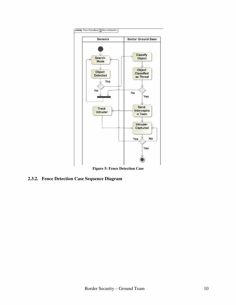
2.3. Use Case 2 – Fence Detection Case

• Description: All Fence sensors in sector are on and tracking intruder • Primary Actors: Intruder, Authorized Personal, Environment • Preconditions: Intruder Detected • Flow of Events:

1. Sensors detects intruder 2. Communicate to ground base 3. All sensors in sector turn on and track intruder 4. Wait for interrupt

2.3.1. Fence Detection Case Activity Diagram


Figure 5: Fence Detection Case

2.3.2. Fence Detection Case Sequence Diagram


Figure 6: Fence Detection Case

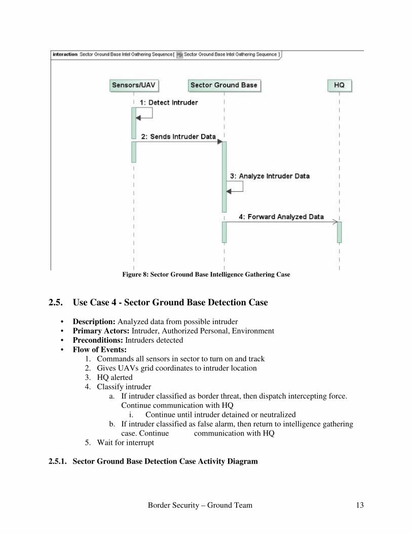
2.4. Use Case 3 - Sector Ground Base Intelligence Gathering Case

• Description: Data from UAV and Fence is being gathered and analyzed • Primary Actors: Intruder, Authorized Personal, Environment, UAV • Preconditions: No previous intruders detected • Flow of Events:

1. All communications open between UAVs and Fence 2. Analyze information received 3. Forward information to HQ 4. Wait for interrupt

2.4.1. Sector Ground Base Intelligence Gathering Case Activity Diagram


Figure 7: Sector Ground Base Intelligence Gathering Case

2.4.2. Sector Ground Base Intelligence Gathering Case Sequence Diagram


Figure 8: Sector Ground Base Intelligence Gathering Case

2.5. Use Case 4 - Sector Ground Base Detection Case

• Description: Analyzed data from possible intruder • Primary Actors: Intruder, Authorized Personal, Environment • Preconditions: Intruders detected • Flow of Events:

1. Commands all sensors in sector to turn on and track 2. Gives UAVs grid coordinates to intruder location 3. HQ alerted 4. Classify intruder

a. If intruder classified as border threat, then dispatch intercepting force. Continue communication with HQ

i. Continue until intruder detained or neutralized b. If intruder classified as false alarm, then return to intelligence gathering

case. Continue communication with HQ 5. Wait for interrupt

2.5.1. Sector Ground Base Detection Case Activity Diagram


Figure 9: Sector Ground Base Detection Case

2.5.2. Sector Ground Base Detection Case Sequence Diagram


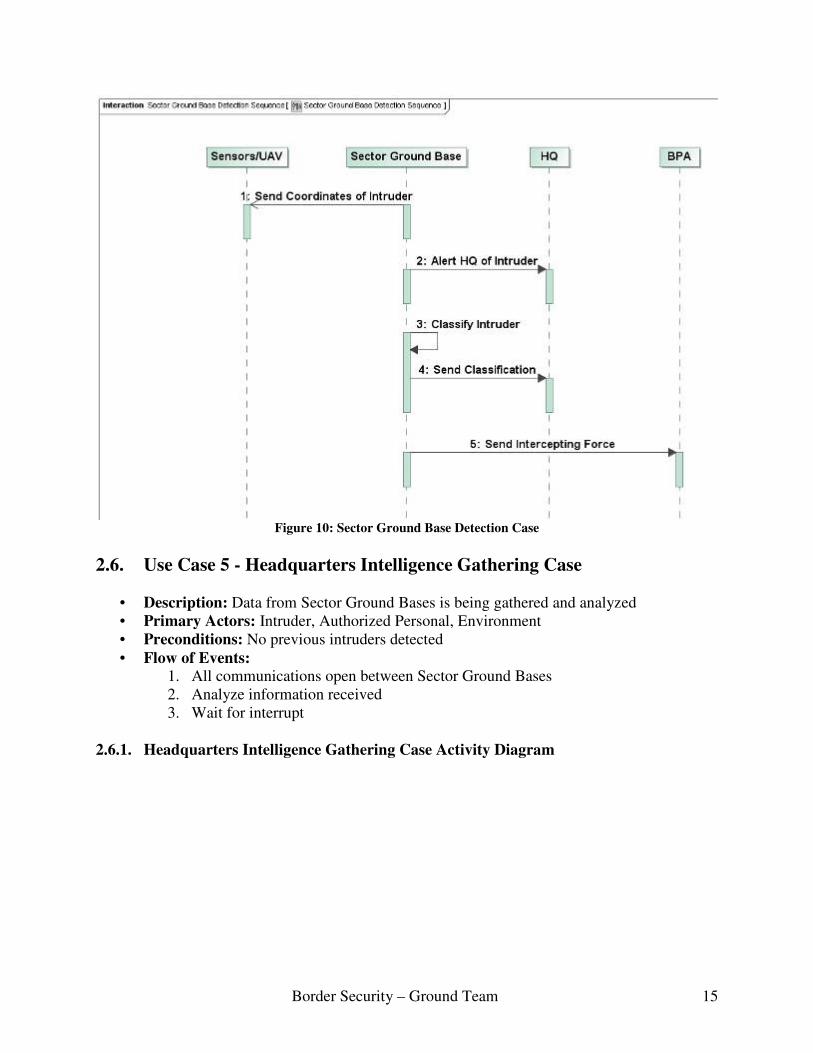
Figure 10: Sector Ground Base Detection Case

2.6. Use Case 5 - Headquarters Intelligence Gathering Case

• Description: Data from Sector Ground Bases is being gathered and analyzed • Primary Actors: Intruder, Authorized Personal, Environment • Preconditions: No previous intruders detected • Flow of Events:

1. All communications open between Sector Ground Bases 2. Analyze information received 3. Wait for interrupt

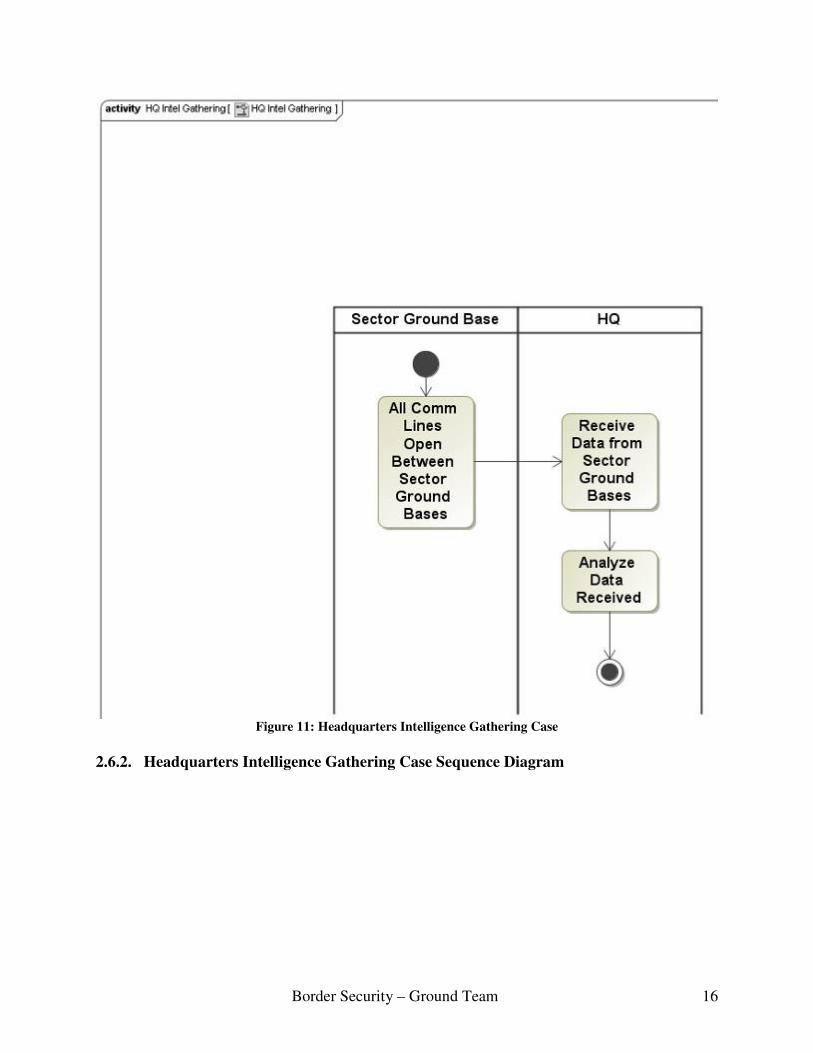
2.6.1. Headquarters Intelligence Gathering Case Activity Diagram


Figure 11: Headquarters Intelligence Gathering Case

2.6.2. Headquarters Intelligence Gathering Case Sequence Diagram


Figure 12: Headquarters Intelligence Gathering Case

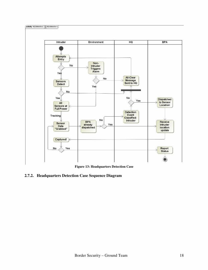
2.7. Use Case 6 - Headquarters Detection Case

• Description: Sector Ground Base reports intruder • Primary Actors: Intruder, Authorized Personnel, Environment • Preconditions: Intruder(s) detected • Flow of Events:

1. Classify intruder a. If intruder classified as border threat, then dispatch intercepting force.

Continue communication with HQ i. Continue until intruder detained or neutralized

b. If intruder classified as false alarm, then return to intelligence gathering case. Continue communication with HQ

2. Wait for interrupt 2.7.1. Headquarters Detection Case Activity Diagram


Figure 13: Headquarters Detection Case

2.7.2. Headquarters Detection Case Sequence Diagram


Figure 14: Headquarters Detection Case

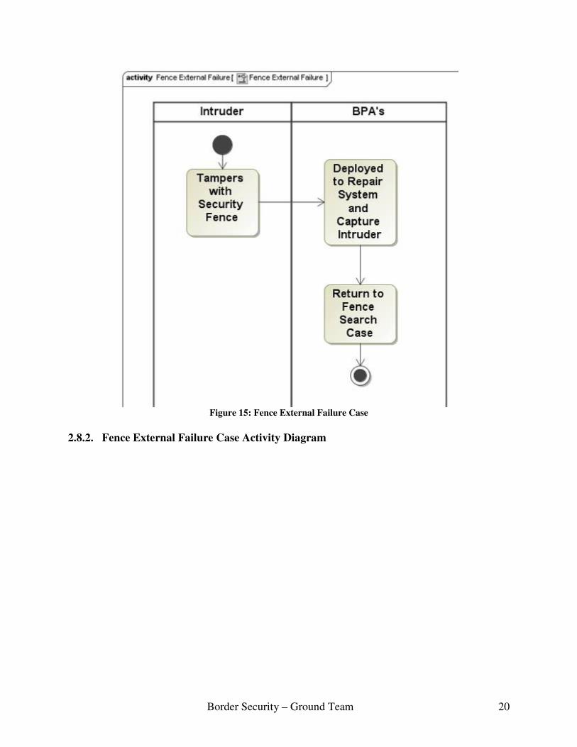
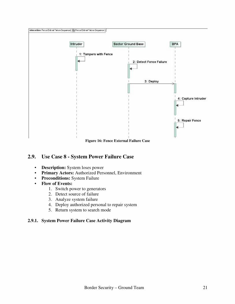
2.8. Use Case 7 - Fence External Failure Case

• Description: Intruder disables security system

• Primary Actors: Intruder, Authorized Personal • Preconditions: System Failure • Flow of Events:

1. Alert BPA of tampering 2. Deploy BPA

a. Repair damaged system b. Track and capture intruder

3. Return system to search mode 2.8.1. Fence External Failure Case Activity Diagram


Figure 15: Fence External Failure Case

2.8.2. Fence External Failure Case Activity Diagram


Figure 16: Fence External Failure Case

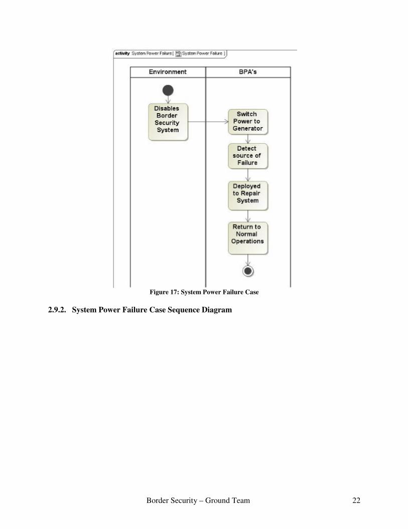
2.9. Use Case 8 - System Power Failure Case

• Description: System loses power

• Primary Actors: Authorized Personnel, Environment • Preconditions: System Failure • Flow of Events:

1. Switch power to generators 2. Detect source of failure 3. Analyze system failure 4. Deploy authorized personal to repair system 5. Return system to search mode

2.9.1. System Power Failure Case Activity Diagram


Figure 17: System Power Failure Case

2.9.2. System Power Failure Case Sequence Diagram


Figure 18: System Power Failure Case

2.10. Use Case 9 - Border Patrol Agent Tracking Case

• Description: Detected intruder is tracked by BPA

• Primary Actors: Intruder, Authorized Personal, Environment • Preconditions: Intruder(s) detected and confirmed, BPA agent deployed • Flow of Events:

1. BPA receives intruder’s detection info 2. BPA is deployed 3. Agent tracks and captures intruder

2.10.1. Border Patrol Agent Tracking Case Activity Diagram


Figure 19: Border Patrol Agent Tracking Case

2.10.2. Border Patrol Agent Tracking Case Sequence Diagram


Figure 20: Border Patrol Agent Tracking Case


3. Requirements Engineering This section outlines the requirements placed on our system.

3.1. Requirements Based on our use cases, we created several broad requirements for the border system’s structure and behavior. After these high-level requirements were finalized, we developed specific conditions that the system would need to meet in order to satisfy the requirements. Table 1 lists these requirements and their associated conditions.

Requirement Description

1 The border must be protected from unauthorized crossings.

a. Seismic fiberoptic sensors shall be used to detect attempts to tunnel across the border

b. Vibration sensors shall be used to detect attempts to cut through or destroy the

border fence

c. Visual spectrum/night vision capable cameras shall be used to detect above ground

approaches to the border

d. Thermal imaging cameras shall be used to detect above ground approaches to the

border

e. Areas of the border not spanned by fence shall be monitored by ground based

sensors or patrolled by UAV

f. Border Patrol Agents (BPA) must be able to track intruder movements using the

active sensors in their sector

2 System must classify crossing attempts as authorized or unauthorized

a. Intruder classification and determination will be conducted by border patrol agents

within sector ground base

b. Visual spectrum/night vision capable cameras shall be used to make positive

identification when a crossing attempt is detected.

3 System must record classified crossing attempts for future use

a. System must allow authorized crossings and record date of immigration for future


use

b. System must track unauthorized intruders and record date and time of intrusion for future use

System must be reliable

a. Seismic fiberoptic sensors must have POD > 80%, PFA< 10%

b. Vibration sensors must have POD > 90%, PFA < 2%

4

c. It shall be impossible to disrupt the normal functioning of any sensor without

triggering failure alert in sector ground base

5 System must interface with existing ground facilities

a. System power requirements must not exceed existing border power generation

capabilities

A1. All sensors must assume low-power passive search state when not activated

b. Sector Ground Bases and Ground Headquarters shall be housed in existing sector

stations where available.

6 System must facilitate communication between ground facilities

a. Sector Ground Bases shall be linked by wired and satellite communication to

Ground Headquarters

b. All sensors within a sector shall be linked by wired communication to the Sector Ground Base

7 System must withstand environmental conditions

a. Seismic fiberoptic sensor must be resistant to inference by dirt, water, and

subterranean wildlife

b. Thermal imaging and visual spectrum/night vision capable cameras must be

capable of positive identification in inclement weather, including precipitation and

wind gusts <100 mph

c. Cameras and vibration sensors must be fully operational in temperatures ranging


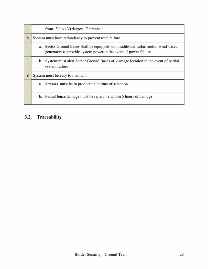
3.2. Traceability

from -30 to 130 degrees Fahrenheit

8 System must have redundancy to prevent total failure

a. Sector Ground Bases shall be equipped with traditional, solar, and/or wind-based

generators to provide system power in the event of power failure

b. System must alert Sector Ground Bases of damage location in the event of partial

system failure

9 System must be easy to maintain

a. Sensors must be in production at time of selection

b. Partial fence damage must be reparable within 5 hours of damage


Component Use Case Requirement Structure/Behavior Description

Fence Search-1 2a behavior High POD, Low Pfa

Fence Detection-1

2a behavior High POD, Low Pfa

Fence Detection- 3

3a behavior Classification determined by BPA

Sensor Behavior Requirements

UAV Search-1 2b behavior UAV searches areas of the border not

spanned by fence or monitored by ground

based sensors

Sensor Structure Requirements

Fence Search -2

Fence Detection -2

9b Structure

GS Analysis-1 9b Structure

GS Classification-1

9b Behavior

All sensors within a sector will be connected via

communication network to the sector

ground base

GS Analysis-2 3a Behavior Intruder classification and determination

will be conducted by border patrol agents within sector ground

base

GS Analysis- 3 9a Structure

Ground Sector Station

Requirements

GS Classification-3

9a Structure

Sector ground bases shall be linked by

wired and communication to

Ground Headquarters

Ground Sector HQ

HQ Analysis-1 9a Structure GS and HQ maintain open communication

GS Classification –

4.1

6a Behavior Date, time, and nature of all confirmed attempts to cross border shall be

recorded for future use by border patrol

agents

GS Classification-

4.2

5 Behavior System should allow authorized crossings and keep records of

immigration for future use by BPA

Border Patrol Agent

BPA Tracking 1a Behavior Agents should be able to track intruder

movements using the


active sensors in their sector

Fence -1 4c Structure/Behavior It shall be impossible to disrupt the normal functioning of any

sensor without triggering failure alert in sector ground base

Reliability

12a Behavior System should maintain operational

state without continuous access to

electrical grid

10a Structure Seismic fiberoptic sensor should be

resistant to inference by dirt, water, and

subterranean wildlife

10b Structure Thermal imaging and visual spectrum/night

vision capable cameras will be

resistant to wind gusts <100 mph,

precipitation

Performance Metrics

10c Structure Cameras and vibration sensors should be fully

operation in temperatures -30 to

130 F

Maintenance Fence Search-1 11a Behavior All sensors should assume low-power passive search state when not activated

13a Structure System should stay within designated federal budget and

time constraints

Customer Constraints

13b Structure Sensors will be off-the-shelf components


4. System-Level Design This section outlines our system structure.

4.1. System Structure Diagrams Figure 21 shows a general structure for the entire border security system.

Figure 21: General Structure Diagram of Border Security System

Figure 22 is a slightly more zoomed in form showing types of sensors and small differences between ground sector bases.


Figure 22: Zoomed in Form of Structure Diagram

4.2. System Level Diagram


Figure 23: System Level Diagram


5. Simplified Approach to Trade-off Analysis This section outlines how we chose which sensors to incorporate into our system.

5.1. Trade-off Analysis Our bases for trade-off are three metrics that determine what type and how many sensors will be used to secure the border. These metrics are:

• Cost

• Power consumption

• Probability of detection Thus, we would want to minimize cost and power consumption and maximize probability of detection. Sensors: we have chosen four sensors from each category of: Thermal camera/sensor Daylight camera/sensor Fence vibration sensor Underground fiber optic sensor Cost matrix: the cost matrix is a 4x4 matrix that holds the values for the costs of the sensors. The four elements of each row are costs (in dollars) for sensors of the same type. Cost matrix = [25000, 45000, 50000, 70000] [500, 76000, 300, 48400] [240, 4620, 1200, 200] [300000, 64000, 50712, 150000] Power matrix: Just as the cost matrix, the power matrix is also a 4x4 matrix in which the four elements of each row are power consumption values (in Watts) for sensors of the same type. Power matrix = [100, 125, 250, 300] [18, 400, 18, 9] [.42, 12, 28, 4] [350, 50, 12, 20] Probability of detection (POD): the POD matrix is also a 4x4 matrix in which the four elements of the each row of the matrix are the POD (in %) for sensors of the same type. POD matrix = [80, 85, 90, 95] [85, 98, 80, 95]


[83, 95, 90, 80] [90, 87, 89, 90] Trade-off Approach: the trade-off approach is to optimize for one metric at a time. Optimizing cost Find all possible cost combinations between the different types of sensors and take their sum. [Note: for a 4x4 matrix there would be 256 possible combinations] Plot sums of the combinations with respect to the corresponding combinations of that of the power matrix. Do the same with respect to the POD matrix. Find the points closest to the axis representing the cost for both cost versus power and cost versus POD plots. Theses point optimize for cost in both plots. Optimizing power Find all possible power combinations between the different types of sensors and take their sum. Plot sums of the combinations with respect to the corresponding combinations of that of the POD matrix. Find the point closest to the axis representing the power. [Note: that the cost versus power plot has already been generated when optimizing cost so the closes point to the power axis can be found from that plot] Optimizing POD [Note: the plots cost versus POD and power versus POD, have already been generated from the previous two optimizations for cost and power. Those plots can be used to find the closest (or the optimal) points to the POD axis. Alternate Optimization approach Using a 3D plot, the combinations for the cost, power and POD can be plotted together. Then the closest points to each planar axis can be found for cost, power, and POD. Methodology for optimization A Matlab code was used to carry out the optimization. The algorithm of the code is as follows: Generate all possible combinations of the three matrices using 4 nested loops. Sum the combinations inside the most inner loop in the nested loop structure for each matrix and collect the results in 3 independent arrays that correspond to cost, power and POD, while keeping track of the combinations in 3 different 4x256 matrices for further analysis later. Use the ‘plot’ matlab function to graph cost vs. power, power vs. POD, and POD vs. cost independently.


Find the minimal sums inside all three arrays using the ‘min’ matlab function to identify the optimal points for all the three metrics. Identify the coordinates of those points in the plot. Find which combination of sensors/cameras give result to the optimal points inside the graph using search algorithms. Here, the combination matrices from (2) will be of great use to find the desired optimal combinations. The methodology described above is not exhaustive. Other complex algorithms were used when weighting the points and finding the dominant ones. As a result we were able to generate plots that were better in showing the set of points of interest that would help in the final process of selecting the optimal point(s) that consider all metrics. Also using the ‘norm’ matlab function we were able to determine a set of the points that were close to the origin with a certain boundary of distance and see if any of the optimal points we found were in the set to ultimately find exhaustive optimal points. An alternate methodology used is a 3D plot of the points collected in (2) using a source code for a function named ‘plot3k’ written by Ken Garrard from North Carolina State University. [The matlab code can be found online look in the appendix for the URL]. With this methodology all three metrics can have one plot and 3 points (out of 256) that represent optimal points for cost, power and POD independently. The Matlab Code can be found in the Appendix Results of trade-off analysis


0.5 1 1.5 2 2.5 3 3.5 4 4.5 5

x 105

100

200

300

400

500

600

700

800

900

1000Power Vs. Cost

Cost ($)

Pow

er

(Watt

s)

Figure 24: Power vs. Cost

Note: The different colors do not have much significance. They only represent combinations the cost and power matrix generated at different iterations in the nested for loop structure in the matlab code.


0.6 0.8 1 1.2 1.4 1.6 1.8 2 2.2 2.4 2.6

x 105

120

140

160

180

200

220

240

Cost ($)

Pow

er

(Watt

s)

(124352,1.214200e+002)

(76212,134)

Power Vs. Cost

Figure 25: Power vs. Cost

This plot shows a reduced number of points generated by weighting – finding the dominant points. As can be seen in the plot the two independent points that optimize for cost and power are ($76212, 134W) and ($124352, 121.42W) respectively. These are the results of the following combinations: Optimizing for cost Cost combination: [25000, 300, 200, 50712] Power combination: [100, 18, 4, 12] [HRC-E series, LONG RANGE - High Resolution – Zoom, IntelliFiber 4+2 core, Fiber SenSys FD525] Optimizing for power Cost combination: [25000, 48400, 240, 50712] Power combination: [100, 9, 0.42, 12] respectively. [HRC-E series, EV-3000 DUAL LONG RANGE DAY/ NIGHT CAMERA, RBtec SL-3, Fiber SenSys FD525] The point with the least norm is: (76212, 134)


100 200 300 400 500 600 700 800 900 1000 1100

80

85

90

95

Average Probability of Detection vs. Power

Power(Watts)

Avera

ge P

robabilt

iy o

f D

ete

ction (

%)

Figure 26: POD vs. Power


100 200 300 400 500 600 700 800 900 1000 1100

82

84

86

88

90

92

94

96

Average Probability of Detection vs. Power

Power (Watts)

Avera

ge P

robabili

ty o

f D

ete

ction (

%)

(732,9.450000e+001)

(1.214200e+002,8.675000e+001)

Figure 27: POD vs. Power


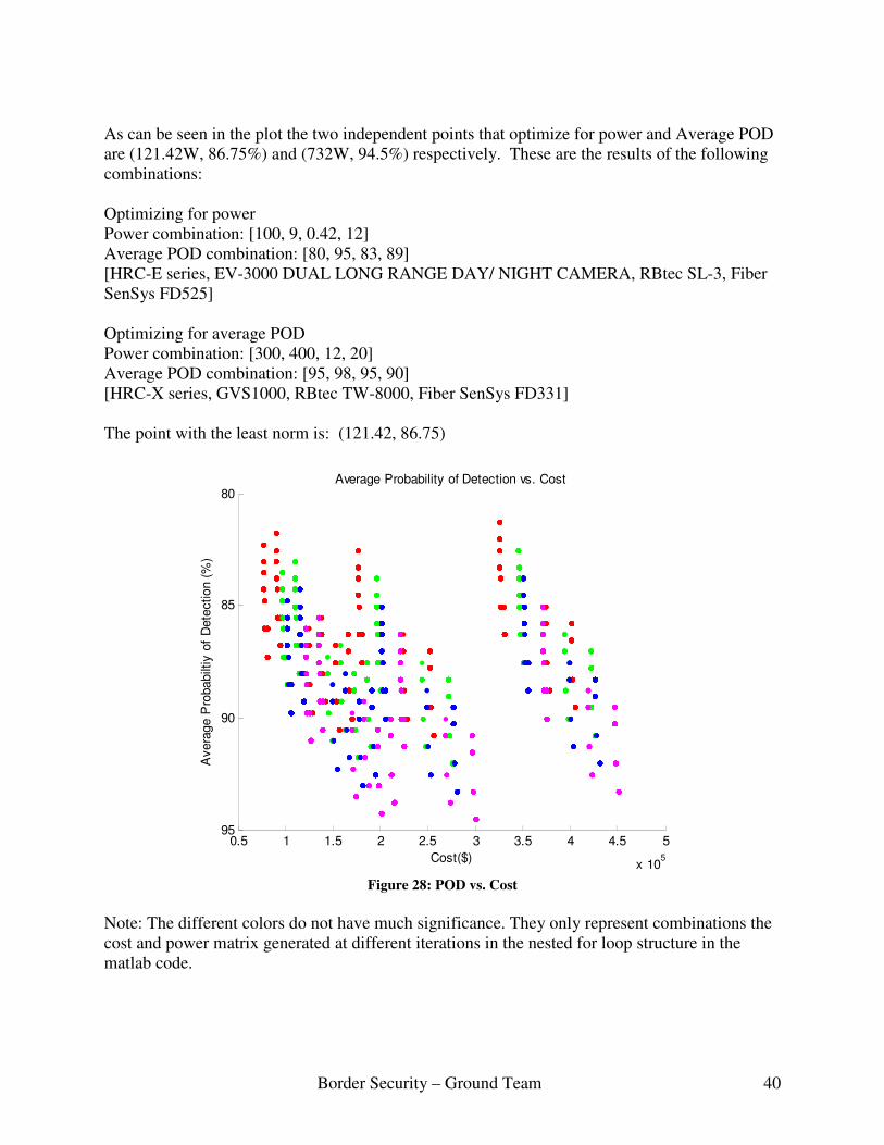
As can be seen in the plot the two independent points that optimize for power and Average POD are (121.42W, 86.75%) and (732W, 94.5%) respectively. These are the results of the following combinations: Optimizing for power Power combination: [100, 9, 0.42, 12] Average POD combination: [80, 95, 83, 89] [HRC-E series, EV-3000 DUAL LONG RANGE DAY/ NIGHT CAMERA, RBtec SL-3, Fiber SenSys FD525] Optimizing for average POD Power combination: [300, 400, 12, 20] Average POD combination: [95, 98, 95, 90] [HRC-X series, GVS1000, RBtec TW-8000, Fiber SenSys FD331] The point with the least norm is: (121.42, 86.75)

0.5 1 1.5 2 2.5 3 3.5 4 4.5 5

x 105

80

85

90

95

Average Probability of Detection vs. Cost

Cost($)

Avera

ge P

robabilt

iy o

f D

ete

ction (

%)

Figure 28: POD vs. Cost



0.5 1 1.5 2 2.5 3 3.5 4 4.5 5

x 105

82

84

86

88

90

92

94

96

Average Probability of Detection vs. Cost

Cost ($)

Avera

ge P

robabili

ty o

f D

ete

ction (

%)

(76212,8.225000e+001)

(300620,9.450000e+001)

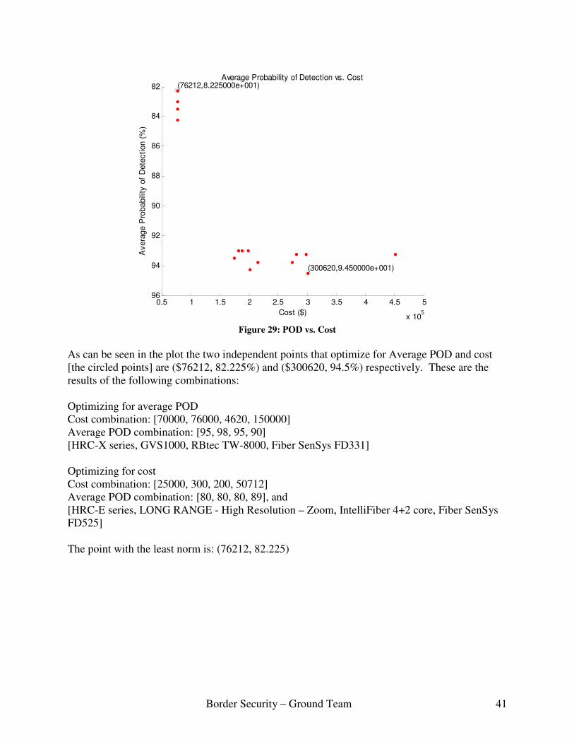
Figure 29: POD vs. Cost

As can be seen in the plot the two independent points that optimize for Average POD and cost [the circled points] are ($76212, 82.225%) and ($300620, 94.5%) respectively. These are the results of the following combinations: Optimizing for average POD Cost combination: [70000, 76000, 4620, 150000] Average POD combination: [95, 98, 95, 90] [HRC-X series, GVS1000, RBtec TW-8000, Fiber SenSys FD331] Optimizing for cost Cost combination: [25000, 300, 200, 50712] Average POD combination: [80, 80, 80, 89], and [HRC-E series, LONG RANGE - High Resolution – Zoom, IntelliFiber 4+2 core, Fiber SenSys FD525] The point with the least norm is: (76212, 82.225)


0

2

4

6

x 105

80

85

90

95

0

200

400

600

800

1000

Cost

Cost vs. Power vs. Probability of Detection

P.O.D

Po

wer

-5.00E-001

-4.00E-001

-3.00E-001

-2.00E-001

-1.00E-001

0.00E+000

1.00E-001

2.00E-001

3.00E-001

4.00E-001

5.00E-001

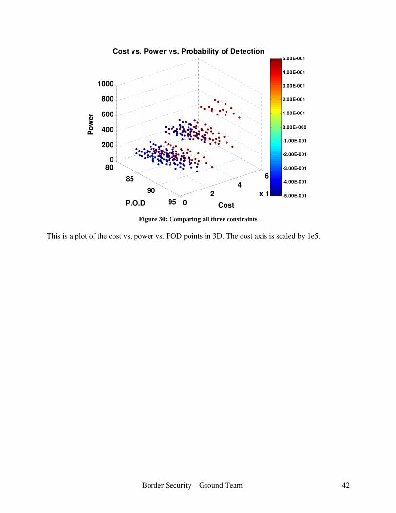
Figure 30: Comparing all three constraints

This is a plot of the cost vs. power vs. POD points in 3D. The cost axis is scaled by 1e5.


0

2

4

6

x 105

80

85

90

95

0

500

1000

1500

(300620,9.450000e+001,732)

Cost

Cost vs. Power vs. Probability of Detection

(124352,8.675000e+001,1.214200e+002)

P.O.D

(76212,8.225000e+001,134)

Po

we

r

-5.00E-001

-4.00E-001

-3.00E-001

-2.00E-001

-1.00E-001

0.00E+000

1.00E-001

2.00E-001

3.00E-001

4.00E-001

5.00E-001

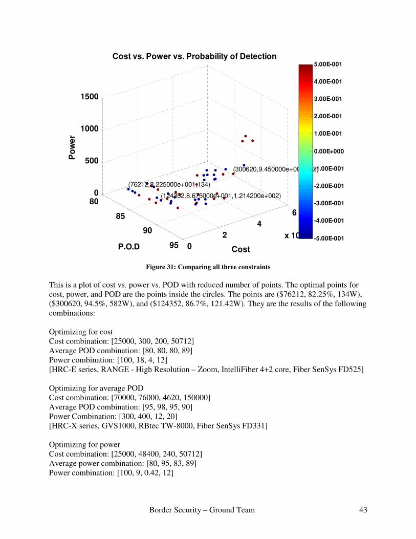
Figure 31: Comparing all three constraints

This is a plot of cost vs. power vs. POD with reduced number of points. The optimal points for cost, power, and POD are the points inside the circles. The points are ($76212, 82.25%, 134W), ($300620, 94.5%, 582W), and ($124352, 86.7%, 121.42W). They are the results of the following combinations: Optimizing for cost Cost combination: [25000, 300, 200, 50712] Average POD combination: [80, 80, 80, 89] Power combination: [100, 18, 4, 12] [HRC-E series, RANGE - High Resolution – Zoom, IntelliFiber 4+2 core, Fiber SenSys FD525] Optimizing for average POD Cost combination: [70000, 76000, 4620, 150000] Average POD combination: [95, 98, 95, 90] Power Combination: [300, 400, 12, 20] [HRC-X series, GVS1000, RBtec TW-8000, Fiber SenSys FD331] Optimizing for power Cost combination: [25000, 48400, 240, 50712] Average power combination: [80, 95, 83, 89] Power combination: [100, 9, 0.42, 12]


[HRC-E series, EV-3000 DUAL LONG RANGE DAY/ NIGHT CAMERA, RBtec SL-3, Fiber SenSys FD525] The point with the least norm is: (76212, 82.25, 134) Final Result

Based on the results from the trade-off analysis shown in the 2D and 3D plots and their respective analysis, the most dominant point that optimizes for all the metrics: cost, power, and POD is: ($76212, 82.25%, 134W). This point can be found in the 3D plot shown Fig 31. This point has the least norm and hence it minimizes cost and power and maximizes the POD. The camera combination that gives result to this point is: Thermal camera/sensor: HRC-E series Daylight camera/sensor: RANGE - High Resolution – Zoom Fence vibration sensor: IntelliFiber 4+2 core Underground fiber optic sensor: Fiber SenSys FD525


6. General Conclusions This problem was quite challenging to our team, and in hindsight, we should have chosen a project on a smaller scale so that we could more easily grasp the concepts of systems engineering. Because the project was on such a large scale we had to dramatically simplify our approach; it also became quite clear to us why Boeing was unable to create a cost effective system that was capable of securing the entire U.S. border. If we were to continue from here we would research our sensors more and perform another trade-off analysis to see how many sensors would be needed to survey the entire border. This would provide us with an overall cost to implement the system. We would also look at how we would operate with the Air Team and their UAVs.


Appendix

A. Matlab Code for Trade-off Analysis – Power vs. Cost

function y = hi2 clear close all

A = [25000 45000 50000 70000]; %thermal B= [500 76000 300 48400];%regular C= [240 4620 1200 200];%vibration D= [300000 64000 50712 150000];%fiber

%power matrix Apow = [100 125 250 300]; Bpow = [18 400 18 9]; Cpow = [.42 12 28 4]; Dpow = [350 50 12 20];

figure(1) title('Power Vs. Cost') m=1; %the following nested loop generates the combination of cost and power

matricies for i = 1:4

for j= 1:4

for k=1:4

for l =1:4

X(m) = [A(i)+B(j)+C(k)+D(l)]; Y(m) = [Apow(i)+Bpow(j)+Cpow(k)+Dpow(l)];

all(m,:)=[X(m) Y(m)]; combination1All(m,:) = [A(i) B(j) C(k) D(l)]; combination2All(m,:) = [Apow(i) Bpow(j) Cpow(k) Dpow(l)];

if i == 1

Thermal1(m,:)=[X(m) Y(m)]; combination11(m,:) = [A(i) B(j) C(k) D(l)]; combination12(m,:) = [Apow(i) Bpow(j) Cpow(k) Dpow(l)]; end if i ==2

Thermal2(m,:)=[X(m) Y(m)]; combination21(m,:) = [A(i) B(j) C(k) D(l)];


combination22(m,:) = [Apow(i) Bpow(j) Cpow(k) Dpow(l)]; end if i==3

Thermal3(m,:)=[X(m) Y(m)]; combination31(m,:) = [A(i) B(j) C(k) D(l)]; combination32(m,:) = [Apow(i) Bpow(j) Cpow(k) Dpow(l)]; end if i==4

Thermal4(m,:)= [X(m) Y(m)]; combination41(m,:) = [A(i) B(j) C(k) D(l)]; combination42(m,:) = [Apow(i) Bpow(j) Cpow(k) Dpow(l)]; end

m=m+1; end end end end xlabel('Cost ($)');ylabel('Power (Watts)')

hold on k = 1; j = 1; %extract the column vectors from Therml1,Thermal2, Thermal3, Thermal4 for i = 1:64 Thermal_11(i) = Thermal1(i,1); Thermal_12(i) = Thermal1(i,2); plot(Thermal_11,Thermal_12,'.r'); j= i+64; Thermal_21(i) = Thermal2(j,1); Thermal_22(i) = Thermal2(j,2); k = j+64; plot(Thermal_21,Thermal_22,'.g'); Thermal_31(i) = Thermal3(k,1); Thermal_32(i) = Thermal3(k,2); l = k+64; plot(Thermal_31, Thermal_32, '.b'); Thermal_41(i) = Thermal4(l,1); Thermal_42(i) = Thermal4(l,2); plot(Thermal_41, Thermal_42, '.m');

end

%find the optimal (minimal points) from the arrays x1 = min(Thermal_11); y1 = min(Thermal_12); [x1, y1]

x2 = min(Thermal_21); y2 = min(Thermal_22); [x2, y2]




x = [x1 x2 x3 x4]; min1 = min(x); y = [y1 y2 y3 y4]; min2 = min(y);

%find the indicies of the arrays where the optimal point are located for i = 1:64

if(Thermal_11(i) == x1) a1 = i; end if(Thermal_12(i) == y1) b1 = i; Thermal_12(i) end if(Thermal_21(i) == x2) a2 = i; end if(Thermal_22(i) == y2) b2 = i; end

if(Thermal_31(i) == x3) a3 = i; end if(Thermal_32(i) == y3) b3 = i; end if(Thermal_41(i) == x4) a4 = i; end if(Thermal_42(i) == y4) b4 = i; end end

figure title('Power Vs. Cost'); xlabel('Cost ($)');ylabel('Power (Watts)')

hold on

%****************************analysis********************************* %here the dominating optimal points are extracted from Thermal_11, %Thermal_12,....Thermal_42 to ultimately find the points that optimize for %cost and power.


Thermal_lowCost_point1 = Thermal_11(a1); power_at_Point1 = Thermal_12(a1); 'point of lowest thermal cost (cost,power) =' [Thermal_lowCost_point1,power_at_Point1] 'it is a result of the combination' combination11(a1,:) Thermal_lowCost_list(1) = Thermal_lowCost_point1;

Thermal_lowPower_point1 = Thermal_12(b1); Thermal_cost_at_point1 = Thermal_11(b1); 'point of lowest power (cost,power) =' [Thermal_cost_at_point1, Thermal_lowPower_point1] 'it is a result of the combination' Thermal_lowPower_list(1) = Thermal_lowPower_point1;

combination12(b1,:) plot(Thermal_lowCost_point1,power_at_Point1 ,'Og'); plot(Thermal_cost_at_point1,Thermal_lowPower_point1 ,'Om');

Thermal_lowCost_point2 = Thermal_21(a2); power_at_point2 = Thermal_22(a2); 'Point of lowest cost (cost, power)=' [Thermal_lowCost_point2, power_at_point2] 'it is a result of the combination' Thermal_lowCost_list(2) = Thermal_lowCost_point2; combination21(a2+64,:)

Thermal_lowPower_point2 = Thermal_22(b2); Thermal_cost_at_point2 = Thermal_21(b2); 'point of lowest power (cost, power)=' [Thermal_cost_at_point2, Thermal_lowPower_point2] 'it is a result of the combination' Thermal_lowPower_list(2) = Thermal_lowPower_point2; combination22(b2+64,:) plot(Thermal_lowCost_point2,power_at_point2 ,'Oy'); plot(Thermal_cost_at_point2,Thermal_lowPower_point2 ,'Ob');

Thermal_lowCost_point3 = Thermal_31(a3) power_at_Point3 = Thermal_32(a3); 'point of lowest thermal cost (cost, power)=' [Thermal_lowCost_point3,power_at_Point3] 'it is a result of the combination' Thermal_lowCost_list(3) = Thermal_lowCost_point3; combination31(a3+128,:)

Thermal_lowPower_point3 = Thermal_32(b3) Thermal_cost_at_point3 = Thermal_31(b3) 'point of lowest power (cost, power)=' [Thermal_cost_at_point3, Thermal_lowPower_point3] 'it is a result of the combination' Thermal_lowPower_list(3) = Thermal_lowPower_point3; combination32(b3+128,:) plot(Thermal_lowCost_point3,power_at_Point3 ,'Ok'); plot(Thermal_cost_at_point3,Thermal_lowPower_point3 ,'Om');


Thermal_lowCost_point4 = Thermal_41(a4) power_at_Point4 = Thermal_12(a4); 'point of lowest thermal cost (cost, power)=' [Thermal_lowCost_point4,power_at_Point4] 'it is a result of the combination' Thermal_lowCost_list(4) = Thermal_lowCost_point4; combination41(a4+192,:)

Thermal_lowPower_point4 = Thermal_42(b4) Thermal_cost_at_point4 = Thermal_11(b4); 'point of lowest power (cost, power)=' [Thermal_cost_at_point4, Thermal_lowPower_point4] 'it is a result of the combination' Thermal_lowPower_list(4) = Thermal_lowPower_point4; combination42(b4+192,:) plot(Thermal_lowCost_point4,power_at_Point4 ,'Oc'); plot(Thermal_cost_at_point4,Thermal_lowPower_point4 ,'Or');

%*********************results******************

Minimum_Thermal_Low_Cost = min(Thermal_lowCost_list); Minimum_Thermal_Low_Power = min(Thermal_lowPower_list);

for i=1:m-1 Norm(i) = norm(all(i),1); end

min_Norm = min(Norm);

figure; xlabel('Cost ($)');ylabel('Power (Watts)') hold on k=1; for i=1:m-1

%Reduces the number of points on the plot based on relevance to the %constraints. if (all(i,1) < (Minimum_Thermal_Low_Cost+ 5000)||(all(i,2) <

(Minimum_Thermal_Low_Power + 100))) list(k,:) = [all(i,1) all(i,2)]; k = k+1; end %finds the point in the plot with the smalles norm (this is %one approach used to find the optimal point) if(norm(all(i,1),all(i,2)) == min_Norm) x = all(i,1); y = all(i,2); plot(x,y,'Oc'); end %finds the coordinates that optmize for cost if(all(i,1) == Minimum_Thermal_Low_Cost)


power_at_Min_Point = all(i,2); 'Min point of lowest camera cost (cost,power) =' [Minimum_Thermal_Low_Cost,power_at_Min_Point] 'This is a result of the following combination' Camera_combination = combination1All(i,:) Power_Combination = combination2All(i,:) plot(Minimum_Thermal_Low_Cost,power_at_Min_Point ,'Ob'); end %findsthe coordinates that optimize for power if(all(i,2) == Minimum_Thermal_Low_Power) cost_at_Min_Point = all(i,1); 'Min point of lowest Power used(cost,power) =' [cost_at_Min_Point,Minimum_Thermal_Low_Power] 'This is a result of the following combination' Camera_combination=combination1All(i,:) Power_combination = combination2All(i,:) plot(cost_at_Min_Point,Minimum_Thermal_Low_Power ,'Ok');

end

end

%writes the coordinates of the optimal ponts on the 3D graph strValues = strtrim(cellstr(num2str([cost_at_Min_Point

Minimum_Thermal_Low_Power],'(%d,%d)'))); text(cost_at_Min_Point,Minimum_Thermal_Low_Power,strValues,'VerticalAlignment

','bottom');

strValues = strtrim(cellstr(num2str([Minimum_Thermal_Low_Cost

power_at_Min_Point],'(%d,%d)'))); text(Minimum_Thermal_Low_Cost,power_at_Min_Point,strValues,'VerticalAlignment

','bottom');

title('Power Vs. Cost'); plot(list(:,1),list(:,2),'.r') clear X Y Thermal1 Thermal2 Thermal3 Thermal4 i j k l w x y z

%% %UNTITLED Summary of this function goes here % Detailed explanation goes here

end

B. Matlab Code for Trade-off Analysis – Power vs. Probability of

Detection function y = hi4

clear close all


%cost matrix % A= [25000 45000 50000 70000]*10^(-6); %thermal % B= [500 76000 300 48400]*10^(-6);%regular % C= [240 4620 1200 200]*10^(-6);%vibration % D= [9504000 160000 101425 150000]*10^(-6);%fiber Aprob = [80 85 90 95]; %thermal Bprob = [85 98 80 95];%regular Cprob= [83 95 90 80];%vibration Dprob= [85 87 89 90];%fiber

%power matrix Apow = [100 125 250 300]; Bpow = [18 400 18 9]; Cpow = [.42 12 28 4]; Dpow = [350 50 12 20];

figure(1) title('Average Probability of Detection vs. Power') m=1;

for i = 1:4

for j= 1:4

for k=1:4

for l =1:4

% calculates total cost vs total power X(m) = [Apow(i)+Bpow(j)+Cpow(k)+Dpow(l)]; Y(m) = [Aprob(i)+Bprob(j)+Cprob(k)+Dprob(l)]/4;

all(m,:)=[X(m) Y(m)]; combination1All(m,:) = [Apow(i) Bpow(j) Cpow(k) Dpow(l)]; combination2All(m,:) = [Aprob(i) Bprob(j) Cprob(k) Dprob(l)]; %plot power vs cost if i == 1 Thermal1(m,:)=[X(m) Y(m)]; combination11(m,:) = [Apow(i) Bpow(j) Cpow(k) Dpow(l)]; combination12(m,:) = [Aprob(i) Bprob(j) Cprob(k)

Dprob(l)]; end if i ==2 Thermal2(m,:)=[X(m) Y(m)]; combination21(m,:) = [Apow(i) Bpow(j) Cpow(k) Dpow(l)]; combination22(m,:) = [Aprob(i) Bprob(j) Cprob(k)

Dprob(l)];

end if i==3 Thermal3(m,:)=[X(m) Y(m)]; combination31(m,:) = [Apow(i) Bpow(j) Cpow(k) Dpow(l)];


combination32(m,:) = [Aprob(i) Bprob(j) Cprob(k)

Dprob(l)];

end if i==4 Thermal4(m,:)= [X(m) Y(m)]; combination41(m,:) = [Apow(i) Bpow(j) Cpow(k) Dpow(l)]; combination42(m,:) = [Aprob(i) Bprob(j) Cprob(k)

Dprob(l)]; end

m=m+1; end end end end xlabel('Power(Watts)');ylabel('Average Probabiltiy of Detection (%)') set(gca,'YDir','reverse'); %cleaning up %Thermal2 hold on k = 1; j = 1; for i = 1:64 Thermal_11(i) = Thermal1(i,1); Thermal_12(i) = Thermal1(i,2); plot(Thermal_11,Thermal_12,'.r'); j= i+64; Thermal_21(i) = Thermal2(j,1); Thermal_22(i) = Thermal2(j,2); k = j+64; plot(Thermal_21,Thermal_22,'.g'); Thermal_31(i) = Thermal3(k,1); Thermal_32(i) = Thermal3(k,2); l = k+64; plot(Thermal_31, Thermal_32, '.b'); Thermal_41(i) = Thermal4(l,1); Thermal_42(i) = Thermal4(l,2); plot(Thermal_41, Thermal_42, '.m');

end

%plot(all(:,1),all(:,2),'.r')

x1 = min(Thermal_11); y1 = max(Thermal_12); [x1, y1]





x = [x1 x2 x3 x4]; min1 = min(x); y = [y1 y2 y3 y4]; max2 = max(y); %OMG = [Thermal_11' Thermal_12' Thermal_21' Thermal_22' Thermal_31'

Thermal_32' Thermal_41' Thermal_42'] %size(OMG)

for i = 1:64


if(Thermal_31(i) == x3) a3 = i; end if(Thermal_32(i) == y3) b3 = i; end if(Thermal_41(i) == x4) a4 = i; end if(Thermal_42(i) == y4) b4 = i; end end

figure title('Average Probability of Detection vs. Power') hold on

%****************analysis*********************

%x axis1 Thermal_lowPower_point1 = Thermal_11(a1);%xaxis prob_at_Point1 = Thermal_12(a1);%yaxis 'point of lowest thermal cost (cost,power) =' [Thermal_lowPower_point1,prob_at_Point1]%points 'it is a result of the combination'


combination11(a1,:) Thermal_lowPower_list(1) = Thermal_lowPower_point1;

%y axis1 Thermal_HighProb_point1 = Thermal_12(b1);%xaxis Power_at_point1 = Thermal_11(b1);%yaxis 'point of High Probability (power, probability) =' [Power_at_point1, Thermal_HighProb_point1]%points 'it is a result of the combination' Thermal_HighProb_list(1) = Thermal_HighProb_point1;

combination12(b1,:) plot(Thermal_lowPower_point1,prob_at_Point1 ,'Og'); plot(Power_at_point1,Thermal_HighProb_point1 ,'Om');

%x axis1 Thermal_lowPower_point2 = Thermal_21(a2);%xaxis prob_at_Point2 = Thermal_22(a2);%yaxis 'point of lowest thermal cost (cost,power) =' [Thermal_lowPower_point2,prob_at_Point2]%points 'it is a result of the combination' combination21(a2,:) Thermal_lowPower_list(2) = Thermal_lowPower_point2;





combination32(b3,:)


plot(Thermal_lowPower_point3,prob_at_Point3 ,'Og'); plot(Power_at_point3,Thermal_HighProb_point3 ,'Om');




xlabel('Power (Watts)');ylabel('Average Probability of Detection (%)')

%*********************results**************************** '*************************result************************' Minimum_Thermal_Low_Power = min(Thermal_lowPower_list);

Maximum_Thermal_Prob = max(Thermal_HighProb_list); for i=1:m-1 all2 = [all(i,1), 100 - all(i,2)]; Norm(i) = norm(all2); end 'yo yo this is the min ' min_Norm = min(Norm)

figure; title('Average Probability of Detection vs. Power') xlabel('Power (Watts)');ylabel('Average Probability of Detection (%)') hold on k=1; for i=1:m-1

if (all(i,1) < (Minimum_Thermal_Low_Power + 10)||(all(i,2) >

(Maximum_Thermal_Prob-4))) list(k,:) = [all(i,1) all(i,2)]; k = k+1; end


if(Norm(i) == min_Norm) 'min norm is at **********************************=' minNorm = min_Norm a=all(i,:) x = all(i,1); y = all(i,2); plot(x,y,'Og'); end

if(all(i,1) == Minimum_Thermal_Low_Power)

prob_at_Min_Point = all(i,2); 'Min point of power (power,probability of detection) =' [Minimum_Thermal_Low_Power,prob_at_Min_Point] 'This is a result of the following combination' Power_combination = combination1All(i,:) Probability_Combination = combination2All(i,:) plot(Minimum_Thermal_Low_Power,prob_at_Min_Point ,'Ob'); end

if(all(i,2) == Maximum_Thermal_Prob) power_at_Min_Point = all(i,1); 'Max point of high probability(power, probability of detection) =' [power_at_Min_Point,Maximum_Thermal_Prob] 'This is a result of the following combination' Power_Combination=combination1All(i,:) Probability_combination = combination2All(i,:) plot(power_at_Min_Point,Maximum_Thermal_Prob ,'Og'); end

end

%print the coordinates for the optimal points in the 3D plot strValues =

strtrim(cellstr(num2str([power_at_Min_Point,Maximum_Thermal_Prob],'(%d,%d)'))

); text(power_at_Min_Point,Maximum_Thermal_Prob,strValues,'VerticalAlignment','b

ottom');

strValues =

strtrim(cellstr(num2str([Minimum_Thermal_Low_Power,prob_at_Min_Point],'(%d,%d

)'))); text(Minimum_Thermal_Low_Power,prob_at_Min_Point,strValues,'VerticalAlignment

','bottom');

%reverse the Y axis so that the highest probability is closer to the origin set(gca,'YDir','reverse');

plot(list(:,1),list(:,2),'.r') clear X Y Thermal1 Thermal2 Thermal3 Thermal4 i j k l w x y z



end

C. Matlab Code for Trade-off Analysis – Cost vs. Probability of Detection function y = hi5

clear close all

%Prob matrix Aprob = [80 85 90 95]; %thermal Bprob = [85 98 80 95];%regular Cprob= [83 95 90 80];%vibration Dprob= [85 87 89 90];%fiber

%cost matrix A = [25000 45000 50000 70000]; B = [500 76000 300 48400]; C = [240 4620 1200 200]; D = [300000 64000 50712 150000];

%the following nested loop generates the combination of cost and power %matricies, sums the combinations, and stores the combinations and the %sums figure(1) title('Average Probability of Detection vs. Cost') m=1;

for i = 1:4

for j= 1:4

for k=1:4

for l =1:4

% calculates total cost vs total power X(m) = [A(i)+B(j)+C(k)+D(l)]; Y(m) = [Aprob(i)+Bprob(j)+Cprob(k)+Dprob(l)]/4; %hold on all(m,:)=[X(m) Y(m)]; combination1All(m,:) = [A(i) B(j) C(k) D(l)]; combination2All(m,:) = [Aprob(i) Bprob(j) Cprob(k) Dprob(l)]; %plot power vs cost if i == 1


Thermal1(m,:)=[X(m) Y(m)]; combination11(m,:) = [A(i) B(j) C(k) D(l)]; combination12(m,:) = [Aprob(i) Bprob(j) Cprob(k)

Dprob(l)]; end if i ==2


Dprob(l)];

end if i==3


Dprob(l)];

end if i==4

Thermal4(m,:)= [X(m) Y(m)]; combination41(m,:) = [A(i) B(j) C(k) D(l)]; combination42(m,:) = [Aprob(i) Bprob(j) Cprob(k)

Dprob(l)]; end

m=m+1; end end end end xlabel('Cost($)');ylabel('Average Probabiltiy of Detection (%)') set(gca,'YDir','reverse');

hold on k = 1; j = 1;

%extract the column vectors from Therml1,Thermal2, Thermal3, Thermal4 for i = 1:64 Thermal_11(i) = Thermal1(i,1); Thermal_12(i) = Thermal1(i,2); plot(Thermal_11,Thermal_12,'.r'); j= i+64; Thermal_21(i) = Thermal2(j,1); Thermal_22(i) = Thermal2(j,2); k = j+64; plot(Thermal_21,Thermal_22,'.g'); Thermal_31(i) = Thermal3(k,1); Thermal_32(i) = Thermal3(k,2); l = k+64; plot(Thermal_31, Thermal_32, '.b');


Thermal_41(i) = Thermal4(l,1); Thermal_42(i) = Thermal4(l,2); plot(Thermal_41, Thermal_42, '.m');

end

%find the optimal (minimal points) from the arrays x1 = min(Thermal_11); y1 = max(Thermal_12); [x1, y1]




x = [x1 x2 x3 x4]; min1 = min(x); y = [y1 y2 y3 y4]; max2 = max(y);

%find the indicies of the arrays where the optimal point are located for i = 1:64


if(Thermal_31(i) == x3) a3 = i; end if(Thermal_32(i) == y3) b3 = i; end if(Thermal_41(i) == x4) a4 = i; end if(Thermal_42(i) == y4)


b4 = i; end end

figure title('Average Probability of Detection vs. Cost') hold on

%****************************analysis********************************* %here the dominating optimal points are extracted from Thermal_11, %Thermal_12,....Thermal_42 to ultimately find the points that optimize for %cost and power.

Thermal_lowCost_point1 = Thermal_11(a1);%xaxis prob_at_Point1 = Thermal_12(a1);%yaxis 'point of lowest thermal cost (cost,probabability) =' [Thermal_lowCost_point1,prob_at_Point1]%points 'it is a result of the combination' combination11(a1,:) Thermal_lowCost_list(1) = Thermal_lowCost_point1;

%y axis1 Thermal_HighProb_point1 = Thermal_12(b1);%xaxis Cost_at_point1 = Thermal_11(b1);%yaxis 'point of High Probability (Cost, probability) =' [Cost_at_point1, Thermal_HighProb_point1]%points 'it is a result of the combination' Thermal_HighProb_list(1) = Thermal_HighProb_point1;

combination12(b1,:) plot(Thermal_lowCost_point1,prob_at_Point1 ,'Og'); plot(Cost_at_point1,Thermal_HighProb_point1 ,'Om');

%x axis1 Thermal_lowCost_point2 = Thermal_21(a2);%xaxis prob_at_Point2 = Thermal_22(a2);%yaxis 'point of lowest thermal cost (cost,Cost) =' [Thermal_lowCost_point2,prob_at_Point2]%points 'it is a result of the combination' combination21(a2,:) Thermal_lowCost_list(2) = Thermal_lowCost_point2;










xlabel('Cost($)');ylabel('Average Probability of Detection (%)')

%*********************results***************************

Minimum_Thermal_Low_Cost = min(Thermal_lowCost_list); Maximum_Thermal_Prob = max(Thermal_HighProb_list);

for i=1:m-1 all2 = [all(i,1), 100-all(i,2)]; Norm(i) = norm(all2); end


min_Norm = min(Norm);

figure; title('Average Probability of Detection vs. Cost') xlabel('Cost ($)');ylabel('Average Probability of Detection (%)') hold on k=1; for i=1:m-1 %Reduces the number of points on the plot based on relevance to the %constraints. if (all(i,1) < (Minimum_Thermal_Low_Cost + 1000)||(all(i,2) >

(Maximum_Thermal_Prob-2))) k; list(k,:) = [all(i,1) all(i,2)];

k = k+1; end %finds the point in the plot with the smalles norm (this is %one approach used to find the optimal point) if(Norm(i) == min_Norm) 'min norm is at **********************************=' minNorm = min_Norm a=all(i,:) x = all(i,1); y = all(i,2); plot(x,y,'Og');

end %finds the coordinates that optmize for cost if(all(i,1) == Minimum_Thermal_Low_Cost)

prob_at_Min_Point = all(i,2); 'Min point of Cost (Cost,probability of detection) =' [Minimum_Thermal_Low_Cost,prob_at_Min_Point] 'This is a result of the following combination' Cost_combination = combination1All(i,:) Probability_Combination = combination2All(i,:) plot(Minimum_Thermal_Low_Cost,prob_at_Min_Point ,'Ob'); end %finds the coordinates that optmize for POD if(all(i,2) == Maximum_Thermal_Prob) Cost_at_Min_Point = all(i,1); 'Max point of high probability(Cost, probability of detection) =' [Cost_at_Min_Point,Maximum_Thermal_Prob] 'This is a result of the following combination' Cost_Combination=combination1All(i,:) Probability_combination = combination2All(i,:) plot(Cost_at_Min_Point,Maximum_Thermal_Prob ,'Og');

end

end


%print the coordinates for the optimal points in the 3D plot strValues =

strtrim(cellstr(num2str([Minimum_Thermal_Low_Cost,prob_at_Min_Point],'(%d,%d)

'))); text(Minimum_Thermal_Low_Cost,prob_at_Min_Point,strValues,'VerticalAlignment'

,'bottom');

strValues =

strtrim(cellstr(num2str([Cost_at_Min_Point,Maximum_Thermal_Prob],'(%d,%d)')))

; text(Cost_at_Min_Point,Maximum_Thermal_Prob,strValues,'VerticalAlignment','bo

ttom');

%reverse the Y axis so that the highest probability is closer to the origin set(gca,'YDir','reverse');

plot(list(:,1),list(:,2),'.r') clear X Y Thermal1 Thermal2 Thermal3 Thermal4 i j k l w x y z


end

D. Matlab Code for Trade-off Analysis – Power vs. Cost vs. POD function y = hi7

%cost matrix % A= [25000 45000 50000 70000]*10^(-6); %thermal % B= [500 76000 300 48400]*10^(-6);%regular % C= [240 4620 1200 200]*10^(-6);%vibration % D= [9504000 160000 101425 150000]*10^(-6);%fiber

% lists the cost of the cameras Acost=[25000 45000 50000 70000]; Bcost=[500 76000 300 48400]; Ccost = [240 4620 1200 200]; Dcost = [300000 64000 50712 150000];

%lists the Probability of detection for the cameras Aprob = [80 85 90 95]; %thermal Bprob = [85 98 80 95];%regular Cprob= [83 95 90 80];%vibration Dprob= [85 87 89 90];%fiber

%lists the power consumption of the cameras Apow = [100 125 250 300]; Bpow = [18 400 18 9]; Cpow = [.42 12 28 4]; Dpow = [350 50 12 20];


figure(1) title('Average Probability of Detection vs. Cost') m=1;

%nested loop structure is used find all the possible combination of each

different %camera along with the combined cost, power and Probability of detection for i = 1:4

for j= 1:4

for k=1:4

for l =1:4

% calculates total cost, total power X(m) = Acost(i)+Bcost(j)+Ccost(k)+Dcost(l); Y(m) = [Aprob(i)+Bprob(j)+Cprob(k)+Dprob(l)]/4; Z(m) = Apow(i)+Bpow(j)+Cpow(k)+Dpow(l); %hold on all(m,:)=[X(m) Y(m) Z(m)]; combination1All(m,:) = [Acost(i) Bcost(j) Ccost(k) Dcost(l)]; combination2All(m,:) = [Aprob(i) Bprob(j) Cprob(k) Dprob(l)]; combination3All(m,:) = [Apow(i) Bpow(j) Cpow(k) Dpow(l)]; %plot power vs cost if i == 1 %plot(X(m),Y(m),'.r') Thermal1(m,:)=[X(m) Y(m) Z(m)]; combination11(m,:) = [Acost(i) Bcost(j) Ccost(k)

Dcost(l)]; combination12(m,:) = [Aprob(i) Bprob(j) Cprob(k)

Dprob(l)]; combination13(m,:) = [Apow(i) Bpow(j) Cpow(k) Dpow(l)]; end if i ==2 %plot(X(m),Y(m),'.g') Thermal2(m,:)=[X(m) Y(m) Z(m)]; combination21(m,:) = [Acost(i) Bcost(j) Ccost(k)


Dprob(l)]; combination23(m,:) = [Apow(i) Bpow(j) Cpow(k) Dpow(l)]; end if i==3 %plot(X(m),Y(m),'.b') Thermal3(m,:)=[X(m) Y(m) Z(m)]; combination31(m,:) = [Acost(i) Bcost(j) Ccost(k)


Dprob(l)]; combination33(m,:) = [Apow(i) Bpow(j) Cpow(k) Dpow(l)]; end


if i==4 %plot(X(m),Y(m),'.m') Thermal4(m,:)= [X(m) Y(m) Z(m)]; combination41(m,:) = [Acost(i) Bcost(j) Ccost(k)


Dprob(l)]; combination43(m,:) = [Apow(i) Bpow(j) Cpow(k) Dpow(l)]; end

m=m+1; end end end end

%sets the scale for the axis[xmin xmax ymin ymax %axis([5000 3.5e5 80 100 200 1200])

%flips the Y matrix so that optimal points are closer to the origin set(gca,'YDir','reverse');

%plots all points in 3D (x,y,z) plot3k([all(:,1),all(:,2),all(:,3)],gradient(all(:,3)),[-0.5

0.5],{'o',2},11,{'Cost vs. Power vs. Probability of Detection','Cost',

'P.O.D', 'Power'},'FontName','Arial','FontSize',14,'FontWeight','Bold')

Minimum_Thermal_Low_Cost = min(all(:,1)) Maximum_Thermal_Prob = max(all(:,2)) Min_Power = min(all(:,3))

%finds the closest point to the origin (hopefully, the point that reduces %satisfies all three metrics (cost, power and P.O.D) for i=1:m-1 all2 = [all(i,1), 100-all(i,2),all(i,3)]; Norm(i) = norm(all2); end min_Norm = min(Norm)

figure; hold on

k=1; for i=1:m-1

%reduces the number of point to be plotted based on relevance to the %constrains such as money and energy if (all(i,1) < Minimum_Thermal_Low_Cost + 80 || all(i,2) >

Maximum_Thermal_Prob - 3 || all(i,3) < Min_Power + 30) list(k,:) = [all(i,1) all(i,2) all(i,3)]; k = k+1; end

%finds the closes point from the origin


if(Norm(i) == min_Norm) minNorm = min_Norm a=all(i,:) x = all(i,1) y = all(i,2); z = all(i,3); plot3(x,y,z,'Ok'); end

%finds the coordinates of the point that minimizes the cost of cameras if(all(i,1) == Minimum_Thermal_Low_Cost) Prob_at_Min_Point1 = all(i,2); Power_at_Min_Point1 = all(i,3); 'Min point for Cost (Cost,probability of detection) =' [Minimum_Thermal_Low_Cost,Prob_at_Min_Point1,Power_at_Min_Point1] 'This is a result of the following combination' Cost_combination = combination1All(i,:) Probability_Combination = combination2All(i,:) Power_Combination = combination3All(i,:)

plot3(Minimum_Thermal_Low_Cost,Prob_at_Min_Point1,Power_at_Min_Point1,'Oc'); end

%finds the coordinate of the point that maximizes the P.O.D if(all(i,2) == Maximum_Thermal_Prob) Cost_at_Min_Point2 = all(i,1); Power_at_Min_Point2 = all(i,3); 'Max point for probability of detection(Cost, probability of

detection, Power) =' [Cost_at_Min_Point2,Maximum_Thermal_Prob,Power_at_Min_Point2] 'This is a result of the following combination' Cost_Combination=combination1All(i,:) Probability_combination = combination2All(i,:) Power_Combination = combination3All(i,:)

plot3(Cost_at_Min_Point2,Maximum_Thermal_Prob,Power_at_Min_Point2,'Og');

end

%finds the coordinates for the point that results the lowest power %consumption if(all(i,3) == Min_Power) Prob_at_Min_Point3 = all(i,2); Cost_at_Min_Point3 = all(i,1); 'Min point for Power(Cost, probability of detection,Power) =' [Cost_at_Min_Point3,Prob_at_Min_Point3,Min_Power] 'This is a result of the following combination' Cost_Combination=combination1All(i,:) Probability_combination = combination2All(i,:) Power_Combination = combination3All(i,:) plot3(Cost_at_Min_Point3,Prob_at_Min_Point3,Min_Power,'Or' );

end end

set(gca,'YDir','reverse');


%plots a 3D graph of the reduced set of points plot3k([list(:,1),list(:,2),list(:,3)],gradient(list(:,3)),[-0.5

0.5],{'o',2},11,{'Cost vs. Power vs. Probability of Detection','Cost',

'P.O.D', 'Power'},'FontName','Arial','FontSize',12,'FontWeight','Bold')

%writes the coordinates of the optimal ponts on the 3D graph strValues = strtrim(cellstr(num2str([

Minimum_Thermal_Low_Cost,Prob_at_Min_Point1,Power_at_Min_Point1],'(%d,%d,%d)'

))); text(Minimum_Thermal_Low_Cost,Prob_at_Min_Point1,Power_at_Min_Point1,strValue

s,'VerticalAlignment','bottom');

strValues =

strtrim(cellstr(num2str([Cost_at_Min_Point2,Maximum_Thermal_Prob,Power_at_Min

_Point2],'(%d,%d,%d)'))); text(Cost_at_Min_Point2,Maximum_Thermal_Prob,Power_at_Min_Point2,strValues,'V

erticalAlignment','bottom');

strValues =

strtrim(cellstr(num2str([Cost_at_Min_Point3,Prob_at_Min_Point3,Min_Power],'(%

d,%d,%d)'))); text(Cost_at_Min_Point3,Prob_at_Min_Point3,Min_Power,strValues,'VerticalAlign

ment','bottom');

clear X Y Thermal1 Thermal2 Thermal3 Thermal4 i j k l w x y z


end


Bibliography 1. "Thermal Imaging Cameras for Border Security and Coastal Surveillance." Http://www.flir.com. Web. 20 Feb. 2011. <http://www.flir.com/cvs/eurasia /en/content/?id=9652> 2. U.S. Customs and Border Patrol. <http://www.cbp.gov/xp/cgov/border_security/>. 3. “Environmental Assessment Port Isabel/Brownsville Border Patrol Station.” June 2004. <http://www.swg.usace.army.mil/pe-p/Brownsville/PIB_BPS_Final_EA.pdf>. 4. Tactical Remote Sensor Systems Systems-of-Systems. <http://www.marcorsyscom.usmc.mil/sites/cins/Fact%20Books/All_Source/TRSS_SoS.pdf>. 5. "Underground Security Tech to Revolutionize Border Security." Homeland Security News

Wire. 15 Dec. 2010. Web. 21 Feb. 2011. <http://homelandsecuritynewswire.com/underground-security-tech-revolutionize-border-security>. 6. "TiaLinx Launches New Precision Tunnel Detection, Motion Tracking Sensors - Newport Beach, CA - 37 - AmericanTowns.com." AmericanTowns.com: Online Local Community

Network - Connecting The Community Is What We Do Best. 7 Jan. 2010. Web. 21 Feb. 2011. <http://www.americantowns.com/ca/newportbeach/news/tialinx-launches-new-precision-tunnel-detection-motion-tracking-sensors-245137>. 7. Stana, Richard. Secure Border Initiative Fence Construction Costs. Darby, PA: DIANE Publishing, 2009. Print. 8. Chishti, M. and C. Bergeron. “Quiet Demise of the Virtual Fence.” Migration Information

Source. Migration Policy Institute, 15 Feb. 2011. Web. 21 Feb. 2011. 9. Chaimowicz, L., et al. “Experiments in Multirobot Air-Ground Coordination”. Proceedings of

the 2004 International Conference on Robotics and Automation. New Orleans, LA. (2004):4053-4058.Print. 10. Aslam, J., et al. “Tracking a Moving Object with a Binary Sensor Network”. SenSys ’03. n.p. (2003). Print. 11. Office of Border Patrol Tucson Sector. “Environmental Assessment: Pedestrian Fence near Sasabe, Arizona”. Department of Homeland Security. Jul. 2007. Web. 21 Feb 2011. 12. Koslowski, Rey. "Immigration Reforms and Border Security Technologies. "Http ://

borderbattles.ssrc.org. July-Aug. 2006. Web. 22 Feb. 2011. <http:// borderbattles.ssrc.org/Koslowski/index1.html>.


13. University of Arizona College of Engineering. "Engineers test underground border security system between US and Mexico." ScienceDaily14 December 2010. 22 February 2011 <http://www.sciencedaily.com/releases/2010/12/101214100240.htm>. 14. "Inside USA - Border Security - 15 Mar 08 - Pt. 1." Youtube.com. AlJazeeraEnglish, 15 Mar. 2008. Web. 22 Feb. 2011.<http://www.youtube.com/watch?v=rlyb_AcrE88&feature=fvwrel>. 15. Romeo, Rafael. “Smuggler Tunnels Probe for US Border Weakness.” 22 Feb. 2011. <http://www.cnn.com/2011/WORLD/americas/02/21/mexico.border.us/index.html?hpt=C2>. Other Resources Used:

1. http://en.wikipedia.org/wiki/Illegal_immigration_to_the_United_States 2. http://en.wikipedia.org/wiki/Mexico_%E2%80%93_United_States_border 3. http://en.wikipedia.org/wiki/SBInet 4. http://www.aegis-elec.com/products/pentax-pair.html 5. http://www.flir.com/uploadedfiles/Eurasia/MMC/Comm_sec/SS_0021_EN.pdf 6. http://www.rbtec.com/sl3.htm 7. http://www.fiberpatrol.com/index.php 8. Austin, Mark, Baras, John. “Hands-on Systems Engineering Projects: Spring Semester

2011.” College Park, MD.


Sign-off Sheet Jessica Jones___________________________________________________________________

• Requirements

• System Level Diagram

• Trade-off Analysis

• Traceability Matthew Marsh_________________________________________________________________

• Abstract

• Problem Statement

• Sequence Diagrams

• Conclusion Aaron Olszewski________________________________________________________________

• Textual Scenarios

• Activity Diagrams


• Sensor Research Senay Tekle____________________________________________________________________

• Trade-off Analysis

• Sensor Research


• Activity Diagrams Phil Tucci_____________________________________________________________________

• Structure Diagrams

• Use Case Diagrams

• Activity Diagrams

Submission Date: May 12th, 2011

Border Security – Ground Teamaustin/enes489p/projects2011a/...Border Security – Ground Team 1...

Documents

Transcript of Border Security – Ground Teamaustin/enes489p/projects2011a/...Border Security – Ground Team 1...