Bootstrap of Dependent Data in Finance - Chalmerspalbin/BootstrapDependentAndreasSunesson.pdf ·...

CHALMERS∣∣∣GOTEBORG UNIVERSITY

MASTER’S THESIS

Bootstrap of Dependent Data

in Finance

ANDREAS SUNESSON

Department of Mathematical Statistics

CHALMERS UNIVERSITY OF TECHNOLOGY

GOTEBORG UNIVERSITY

Goteborg, Sweden 2011

Thesis for the Degree of Master of Science

Bootstrap of Dependent Data

in Finance

Andreas Sunesson

CHALMERS∣∣∣ GOTEBORG UNIVERSITY

Department of Mathematical Statistics

Chalmers University of Technology and Goteborg University

SE− 412 96 Goteborg, Sweden

Goteborg, August 2011

Bootstrap of Dependent Data in Finance

Andreas Sunesson

August 17, 2011

Abstract

In this thesis the block bootstrap method is used to generate resamples of time series for Value–at–Risk calculation. A parameter to the method is the block length and this parameter is studiedto see what choice of it gives the best results when looking at multi–day Value–at–Risk estimates.A choice of block length of the roughly the same size as the number of days used for Value–at–Riskseems to give the best results.

iii

Acknowledgements

I would like to thank my supervisor, at Chalmers, Patrik Albin for his support during my work.He his an ideal supervisor for a student. Further on i wish to thank Magnus Hellgren and JesperTidblom and the rest of Algorithmica Research AB for their support.

v

Contents

1 Introduction 1

2 Theory 22.1 Basic definitions . . . . . . . . . . . . . . . . . . . . . . . . . . . . . . . . . . . . . . 22.2 Autocorrelation function . . . . . . . . . . . . . . . . . . . . . . . . . . . . . . . . . . 22.3 Serial variance . . . . . . . . . . . . . . . . . . . . . . . . . . . . . . . . . . . . . . . 32.4 QQ–plots . . . . . . . . . . . . . . . . . . . . . . . . . . . . . . . . . . . . . . . . . . 42.5 Kolmogorov–Smirnov test . . . . . . . . . . . . . . . . . . . . . . . . . . . . . . . . . 52.6 Value–at–Risk, VaR . . . . . . . . . . . . . . . . . . . . . . . . . . . . . . . . . . . . 52.7 GARCH . . . . . . . . . . . . . . . . . . . . . . . . . . . . . . . . . . . . . . . . . . . 52.8 Ljung–Box test . . . . . . . . . . . . . . . . . . . . . . . . . . . . . . . . . . . . . . . 62.9 Kupiec–test . . . . . . . . . . . . . . . . . . . . . . . . . . . . . . . . . . . . . . . . . 6

3 Resampling methods 73.1 The IID Bootstrap method . . . . . . . . . . . . . . . . . . . . . . . . . . . . . . . . 73.2 Example of IID Bootstrap shortcomings . . . . . . . . . . . . . . . . . . . . . . . . . 73.3 Block bootstrap . . . . . . . . . . . . . . . . . . . . . . . . . . . . . . . . . . . . . . . 83.4 Example cont. . . . . . . . . . . . . . . . . . . . . . . . . . . . . . . . . . . . . . . . . 83.5 Optimal block length . . . . . . . . . . . . . . . . . . . . . . . . . . . . . . . . . . . . 8

4 Financial timeseries 104.1 Stylized empirical facts . . . . . . . . . . . . . . . . . . . . . . . . . . . . . . . . . . . 104.2 Interest rates . . . . . . . . . . . . . . . . . . . . . . . . . . . . . . . . . . . . . . . . 104.3 The dataset . . . . . . . . . . . . . . . . . . . . . . . . . . . . . . . . . . . . . . . . . 10

5 Implementation 125.1 Optimal block length . . . . . . . . . . . . . . . . . . . . . . . . . . . . . . . . . . . . 125.2 VaR–estimaton by block bootstrap . . . . . . . . . . . . . . . . . . . . . . . . . . . . 125.3 VaR–estimation by stationary bootstrap . . . . . . . . . . . . . . . . . . . . . . . . . 135.4 Implementation of VaR backtest. . . . . . . . . . . . . . . . . . . . . . . . . . . . . . 13

6 Results 146.1 Choice of blocklength . . . . . . . . . . . . . . . . . . . . . . . . . . . . . . . . . . . 146.2 Backtests . . . . . . . . . . . . . . . . . . . . . . . . . . . . . . . . . . . . . . . . . . 186.3 Comments on the results . . . . . . . . . . . . . . . . . . . . . . . . . . . . . . . . . . 20

A C#–code 25

vii

1 Introduction

In financial institutions there is an ever increasing need to estimate the risk of various positions.Today there exists a number of measures available to risk managers. A risk measure made popularby J.P. Morgan is the Value–at–Risk measure, which simply is the a chosen quantile of the lossdistribution. Value–at–Risk quickly became popular in the industry was also soon adopted bythe Basel Committee on Banking Supervision who regulated that a certain amount of capital wasneeded to cover for the risk exposure indicated by the Value–at–Risk measure. Initially, however,Value–at–Risk was based on an assumption of independent normal distributed asset returns, mainlybecause of the simplicity of calculation and the ease of explaining to senior managment. As knownthough, real world assets, in general, are neither normal distributed nor independent.

This way of estimating Value–at–Risk is by the use of a parametric method, assumptions hasbeen made of the underlying asset return process and parameters has been estimated from his-torical data. By the use of a non–parametric model, though, one can drop a lot of these modelassumptions. One such non–parametric model is resampling by the Bootstrap method, initiallyproposed by Efron in 1979 [3]. This non–parametric model assymptotically replicates the densityof the resampled process. The bootstrap method assumes independent asset returns and a problemwith it, if you try to apply it on a dependent time series, is that the resampled series is independent.To correct for this some modifications to the bootstrap method was later proposed.

In this thesis, dependent time series will be used to study extended versions of the bootstrapmethod, the block bootstrap and the stationary bootstrap. The choice of parameters for the meth-ods are of particular interest and are studied for empirical data by different approaches. Also,how does resampling by these methods preserve the autocorrelation structure in the resamples andfurther on Value–at–Risk estimates will be made based on the resamples.

1

2 Theory

2.1 Basic definitions

We begin by looking at an asset with a price process {St}Tt=0, St > 0. We’re now interested in thereturns of this price process. There are a couple of ways to define this, starting with the simple netreturn, Rt defined by

Rt =StSt−1

− 1

Furtheron, define the log return, Xt, t ∈ [1, T ] by

Xt = log(1 +Rt)

= log

(StSt−1

).

If we look at multiperiod returns Rt(`) and Xt(`) we see that they are obtained by multiplyingthe daily simple net returns between the desired days and adding the log returns for the same period.

Further on we need to define the bias and the mean square error of an estimate. Suppose that{Xt}Tt=0 is identically distributed with some common distribution function, G. Suppose also thatin an experiment we get a sample from the previous sequence, {X1 . . . Xn}. Now suppose we’reinterested in the functional relation θ = θ(G) but don’t know the distribution G. We might esti-mate G with G, from the sample {X1 . . . Xn}. That is, G(X1, . . . , Xn). Thus an estimate of θ isgotten by applying G instead of G. Now is this estimate, θ = θ(G) a good one? To check this weintroduce the bias,

Bias(θ) = E[θ]− θ,

which is essentially the average error we make by estimating θ with θ.

Also we introduce the mean square error and define it by

MSE(θ) = E[(θ − θ

)2]= Bias(θ)2 + Var(θ).

2.2 Autocorrelation function

The correlation, between two random variables X and Y , both square integrable, is defined through

ρ(X,Y ) = Cov(X,Y )/√

Cov(X,X)Cov(Y, Y ).

The sample correlation between two samples X = {X1, . . . , Xn} and Y = {Y1, . . . , Yn} with X =1n

∑ni=1Xi and Y = 1

n

∑ni=1 Yi is defined by

ρ(X,Y ) =

∑nk=0(Xk − X)(Yk − Y )√∑n

k=0(Xk − X)2∑n

k=0(Yk − Y )2.

2

For a sample X = {X1 . . . , Xn} it’s correlation with it self, for a lag `, is defined as the auto-correlation function, ”acf”, [12].

ρ` =

∑Ti=`+1

(Xi − X

) (Xi−` − X

)∑Ti=1

(Xi − X

)2 , ` ∈ [0, T − 1]

Here a value of 1 for a specific ` would indicate that there is a perfect correlation between the seriesstarting at day k and the series starting at day k + `. Note that −1 ≤ ρ ≤ 1.

2.3 Serial variance

The sample variance for X = {X1, . . . , Xn} is calculated by

Var(X) =1

n− 1

n∑i=1

X2i −

1

n

(n∑i=1

Xi

)2 .

The reason for dividing by n− 1 instead of n is that this makes Var(X) an unbiased estimator ofthe variance if the process X is IID and stationary.

When looking at multiperiod returns instead, how do we expect the sample variance to change? Ifwe look at k–day changes, the sample size will decrease by a factor k. Thus we expect to see anincrease in the sample variance since it is expected to increase with a decreasing sample.

Now, looking at k–day, non–overlapping, returns, Xi[k]. Assume that they are stationary and IIDand that k divides n evenly. The data set is Y = {Y1, . . . , Yn/k}, where Yi = Xi(k−1)+1 + · · ·+Xik

for i = {1, . . . , n/k}. We thus have n/k number of observations, the sample variance of this sampleis, with an index k indicating the multiperiod returns,

Vark(X) = Var(Y )

=1

n/k − 1

n/k∑i=1

Y 2i −

1

n/k

n/k∑i=1

Yi

2=

1

n/k − 1

n/k∑i=1

(X(i−1)k+1 + · · ·+Xik

)2 − 1

n/k

n/k∑i=1

(X(i−1)k+1 + · · ·+Xik

)2 .

3

Now assume the data is IID and stationary,

E [Vark(X)] = E

1

n/k − 1

n/k∑i=1

(X(i−1)k+1 + · · ·+Xik

)2 − 1

n/k

n/k∑i=1

(X(i−1)k+1 + · · ·+Xik

)2=

k

n− k

n/k∑i=1

E[(X(i−1)k+1 + · · ·+Xik

)2]− k

nE

( n∑i=1

Xi

)2

=k

n− k

n/k∑i=1

(Var

(X(i−1)k+1 + · · ·+Xik

)+ E

[X(i−1)k+1 + · · ·+Xik

]2)

− k

n

Var

(n∑i=1

Xi

)+ E

[n∑i=1

Xi

]2=

k

n− k

(n

k

(Var(Xi) · k + k2E [Xi]

2)− k

n

(n ·Var (Xi) + n2E[Xi]

2))

=k

n− k

(n ·Var (Xi) + nkE [Xi]

2 − k ·Var (Xi)− nkE [Xi]2)

= k ·Var(X1),

we see that the sample variance increases by a factor of k when the sample size decreases by afactor 1/k.

Now if a sample does not show this tendency, apart from random noise, we could be inclinedto say that the sample is not independent.

2.4 QQ–plots

Assume a stationary sample {X1, . . . , Xn}. A quantile–quantile plot, qq–plot, is a visual wayof checking if the data in the sample belongs to a specified distribution. The ordered sample,{X(1), . . . , X(n)}, where X(i) is the i:th largest element, is plotted against the quantiles of thecorresponding inverted density function.(

X(i), F−1(i− 0.5

n

)),i ∈ [1, n]

The qq–plot can also be used to check if two samples come from the same distribution. Assumethat the samples are of equal size, then the corresponding qq–plot is gotten by ordering the twosamples with increasing values and plotting them against each other. If both samples belong tothe same distribution, the plot is expected to lie on a 45◦ line. If the samples are of different sizes,the same principle applies but a form of interpolation between data points is required to make surethe same quantiles are being plotted against each other.

A deviation from the 45◦ linear fit between the two samples would thus indicate that the twosamples does not share the same distribution and it is in this manner the qq–plots will be used inthis thesis. A bad fit will be ”seen” as a rejection of some hypothesis of the samples not havingthe same distribution. This does not imply that they have the same distribution but it will indeedbe an indication of it.

4

2.5 Kolmogorov–Smirnov test

The Kolmogorov–Smirnov test, KS–test, is a hypothesis test that can be used for testing if twosamples belong to the same distribution. The KS–test usually analyzes a data set to check if itcomes from a known distribution. However, in this article we are looking at non–parametric meth-ods and do not want to mix in any assumptions of that the data has a certain distribution function.We will compare the empirical distribution function of the resampled multi–period returns againstthe original series empirical distribution function.

Under the null–hypothesis, the two compared data sets have the same distribution function. Thisis tested by calculating the statistic D = max

x|Fest(x) − Femp(x)|. Under the null–hypothesis,√

n1n2n1+n2

D is Kolmogorov distributed where n1 and n2 are the sample sizes of the first and the

second series. Thus if the largest difference between the distribution functions are too large, thenull–hypothesis is rejected.

2.6 Value–at–Risk, VaR

Value–at–Risk, VaRα(`), is the magnitude of which losses does not exceed, with probability p =1− α, α ∈ [0, 1] in a timespan of ` days. That is, VaRα(`) is defined through

p = P [L(`) ≥ VaRα] ,

where L is the loss function, for example L(`) = − (St+` − St).

This can be rewritten on the form

VaRα(L) = inf {l ∈ R : P (L ≤ l) ≥ α}

Note that VaR has a weak linearity property, that is for σ ∈ (0,∞) and µ ∈ R,

VaRα (σL+ µ) = inf {l ∈ R : P (σL+ µ ≤ l) ≥ α}= inf {l ∈ R : P (L ≤ (l − µ)/σ) ≥ α} ,

substitute k = (l − µ)/σ,

= inf {σk + µ ∈ R : P (L ≤ k) ≥ α}= σ inf {k ∈ R : P (L ≤ k) ≥ α}+ µ

= σVaRα (L) + µ.

The textbook way of calculating VaR makes use of this fact when it assumes normal distributed log–returns. Calculating VaR is then reduced to estimating the mean,µ, and the standard deviation,σ,of the log–returns. That is, at time t, VaRα = S(t)(µ+ σΦ(α)).

2.7 GARCH

A way of estimating volatility, σ2t , in financial time series is by applying a Generalized autoregressiveconditional heteroscedastic, GARCH, model. A GARCH(p, q) model for estimating the volatility

5

is described by

σ2t = α0 +

p∑i=1

αia2t−i +

q∑i=1

βiσ2t−i

where at is zero–mean adjusted log return process described in section 2.1. Also at = σtεt and, inthis thesis, εt ∼ N(0, 1).

From the way the GARCH model is constructed, at each time t, the volatility process σ2t is con-structed from the previous q volatilities, weighted down by the βi–coefficients. Also the processtakes the last p innovation values, at into consideration, weighted down by the αi–coefficients.

To estimate the parameters α0, . . . , αp, β1, . . . , βq from a data sample, one method commonlyused is MLE.

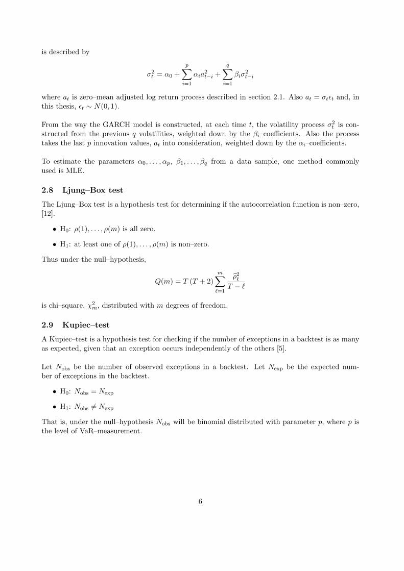
2.8 Ljung–Box test

The Ljung–Box test is a hypothesis test for determining if the autocorrelation function is non–zero,[12].

• H0: ρ(1), . . . , ρ(m) is all zero.

• H1: at least one of ρ(1), . . . , ρ(m) is non–zero.

Thus under the null–hypothesis,

Q(m) = T (T + 2)m∑`=1

ρ2`T − `

is chi–square, χ2m, distributed with m degrees of freedom.

2.9 Kupiec–test

A Kupiec–test is a hypothesis test for checking if the number of exceptions in a backtest is as manyas expected, given that an exception occurs independently of the others [5].

Let Nobs be the number of observed exceptions in a backtest. Let Nexp be the expected num-ber of exceptions in the backtest.

• H0: Nobs = Nexp

• H1: Nobs 6= Nexp

That is, under the null–hypothesis Nobs will be binomial distributed with parameter p, where p isthe level of VaR–measurement.

6

3 Resampling methods

The bootstrap method is a commonly used way of checking the distribution function of someestimator on a time series. Here we give a definition of the method and supply an exampel, withdependent data, where the standard method fails. We then continue to expand the method tobehave descent for dependent data.

3.1 The IID Bootstrap method

The main principle of the bootstrap method is resampling from a known data set, X1, X2, . . . , Xn,to give a distribution of the estimator θ. This is done in the IID Bootstrap–method by pickingn numbers from {1, . . . , n} with equal probability and with replacement. Call a number chosenthis way U to get a sequence Ui, i ∈ [1, n]. Then construct a resample by chosing n data points

XUi , i ∈ [1, n], call this series X1, . . . , Xn and then applying this resample to the estimator θ. By

repeating this process N times we get a series of estimations{θ(X1

j, . . . , Xn

j)}Nj=1

which can be

used to construct a distribution function, P(θ ≤ x

)of θ [1].

The IID Bootstrap–method is based on the idea that the data, X1, X2, . . . , Xn, only representsa single realisation of all possible combinations of that data. The distribution of the estimate θgiven by the IID Bootstrap method is hence an estimate of the distribution of θ if X1, X2, . . . , Xn

came from a common distribution function P (X ≤ x). This however requires the data to be inde-pendent. If the data is in fact dependent, the method fails to give a proper estimate, as seen infollowing example, modified from an article by Eola Investments , LLC [4].

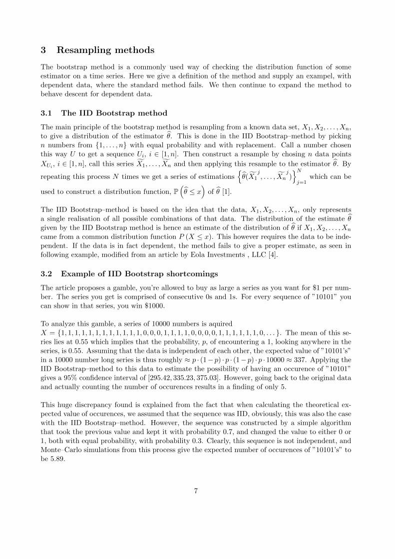
3.2 Example of IID Bootstrap shortcomings

The article proposes a gamble, you’re allowed to buy as large a series as you want for $1 per num-ber. The series you get is comprised of consecutive 0s and 1s. For every sequence of ”10101” youcan show in that series, you win $1000.

To analyze this gamble, a series of 10000 numbers is aquiredX = {1, 1, 1, 1, 1, 1, 1, 1, 1, 1, 1, 1, 0, 0, 0, 1, 1, 1, 1, 0, 0, 0, 0, 1, 1, 1, 1, 1, 1, 0, . . . }. The mean of this se-ries lies at 0.55 which implies that the probability, p, of encountering a 1, looking anywhere in theseries, is 0.55. Assuming that the data is independent of each other, the expected value of ”10101’s”in a 10000 number long series is thus roughly ≈ p · (1− p) · p · (1− p) · p · 10000 ≈ 337. Applying theIID Bootstrap–method to this data to estimate the possibility of having an occurence of ”10101”gives a 95% confidence interval of [295.42, 335.23, 375.03]. However, going back to the original dataand actually counting the number of occurences results in a finding of only 5.

This huge discrepancy found is explained from the fact that when calculating the theoretical ex-pected value of occurences, we assumed that the sequence was IID, obviously, this was also the casewith the IID Bootstrap–method. However, the sequence was constructed by a simple algorithmthat took the previous value and kept it with probability 0.7, and changed the value to either 0 or1, both with equal probability, with probability 0.3. Clearly, this sequence is not independent, andMonte–Carlo simulations from this process give the expected number of occurences of ”10101’s” tobe 5.89.

7

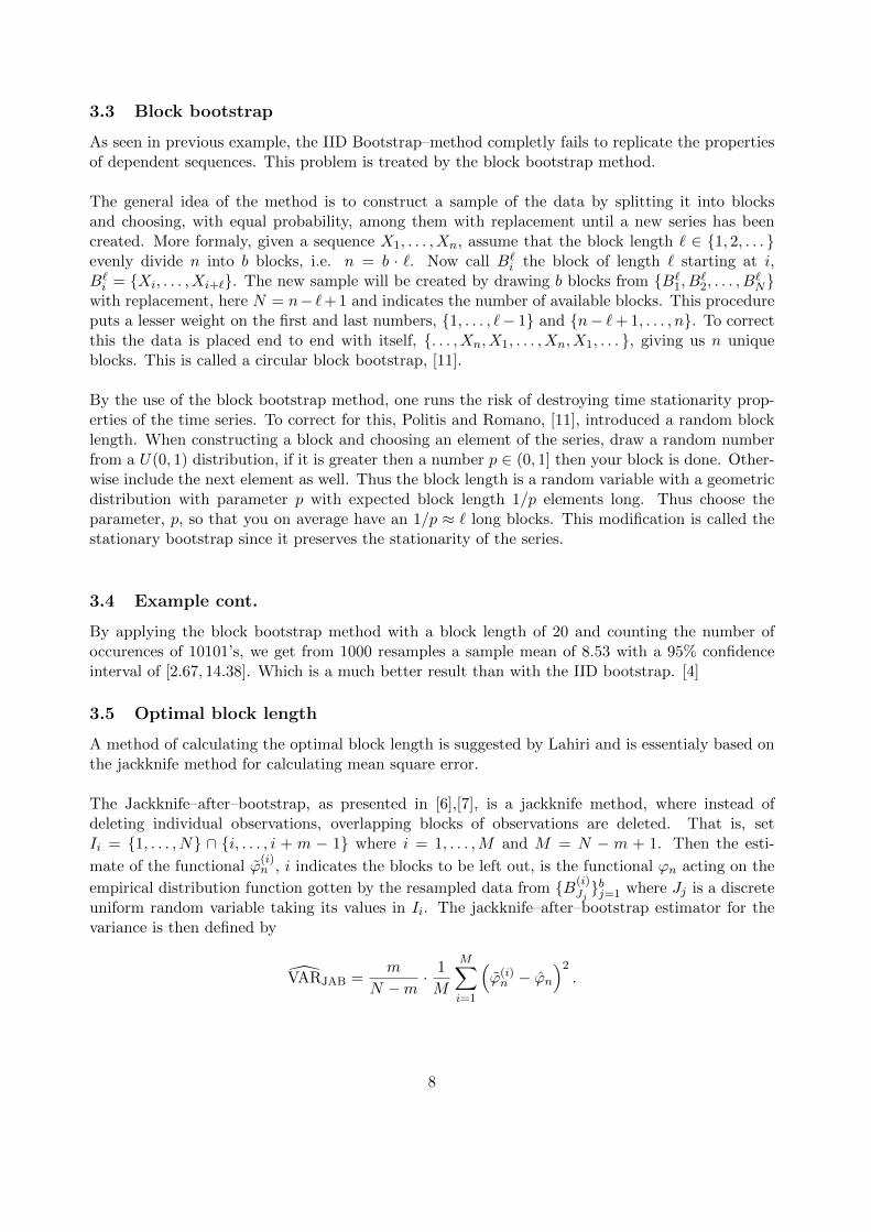
3.3 Block bootstrap

As seen in previous example, the IID Bootstrap–method completly fails to replicate the propertiesof dependent sequences. This problem is treated by the block bootstrap method.

The general idea of the method is to construct a sample of the data by splitting it into blocksand choosing, with equal probability, among them with replacement until a new series has beencreated. More formaly, given a sequence X1, . . . , Xn, assume that the block length ` ∈ {1, 2, . . . }evenly divide n into b blocks, i.e. n = b · `. Now call B`

i the block of length ` starting at i,B`i = {Xi, . . . , Xi+`}. The new sample will be created by drawing b blocks from {B`

1, B`2, . . . , B

`N}

with replacement, here N = n− `+ 1 and indicates the number of available blocks. This procedureputs a lesser weight on the first and last numbers, {1, . . . , `− 1} and {n− `+ 1, . . . , n}. To correctthis the data is placed end to end with itself, {. . . , Xn, X1, . . . , Xn, X1, . . . }, giving us n uniqueblocks. This is called a circular block bootstrap, [11].

By the use of the block bootstrap method, one runs the risk of destroying time stationarity prop-erties of the time series. To correct for this, Politis and Romano, [11], introduced a random blocklength. When constructing a block and choosing an element of the series, draw a random numberfrom a U(0, 1) distribution, if it is greater then a number p ∈ (0, 1] then your block is done. Other-wise include the next element as well. Thus the block length is a random variable with a geometricdistribution with parameter p with expected block length 1/p elements long. Thus choose theparameter, p, so that you on average have an 1/p ≈ ` long blocks. This modification is called thestationary bootstrap since it preserves the stationarity of the series.

3.4 Example cont.

By applying the block bootstrap method with a block length of 20 and counting the number ofoccurences of 10101’s, we get from 1000 resamples a sample mean of 8.53 with a 95% confidenceinterval of [2.67, 14.38]. Which is a much better result than with the IID bootstrap. [4]

3.5 Optimal block length

A method of calculating the optimal block length is suggested by Lahiri and is essentialy based onthe jackknife method for calculating mean square error.

The Jackknife–after–bootstrap, as presented in [6],[7], is a jackknife method, where instead ofdeleting individual observations, overlapping blocks of observations are deleted. That is, setIi = {1, . . . , N} ∩ {i, . . . , i + m − 1} where i = 1, . . . ,M and M = N − m + 1. Then the esti-

mate of the functional ϕ(i)n , i indicates the blocks to be left out, is the functional ϕn acting on the

empirical distribution function gotten by the resampled data from {B(i)Jj}bj=1 where Jj is a discrete

uniform random variable taking its values in Ii. The jackknife–after–bootstrap estimator for thevariance is then defined by

VARJAB =m

N −m· 1

M

M∑i=1

(ϕ(i)n − ϕn

)2.

8

Where ϕ(i)n = (Nϕn − (N −m)ϕ

(i)n )/m. The bias of ϕn is estimated by

Bn = 2`1 (ϕn(`1)− ϕn(2`1))

where `1 is the initial guess of blocklength.

By expansion of the MSE, under some constraints, an estimation of the optimal block lengthis gotten by

˜=

(B2n · n

VARJAB

) 14

.

The exponent 1/4 here comes from the fact that we are looking at one–sided distributions, see forexample [7] and [10].

Further on, a starting value of the block length, `1, and the block of blocks parameter m is sug-gested. A choice of `1 = n

14 and m = 0.1 · (n`21)

13 is said to be optimal, [7].

9

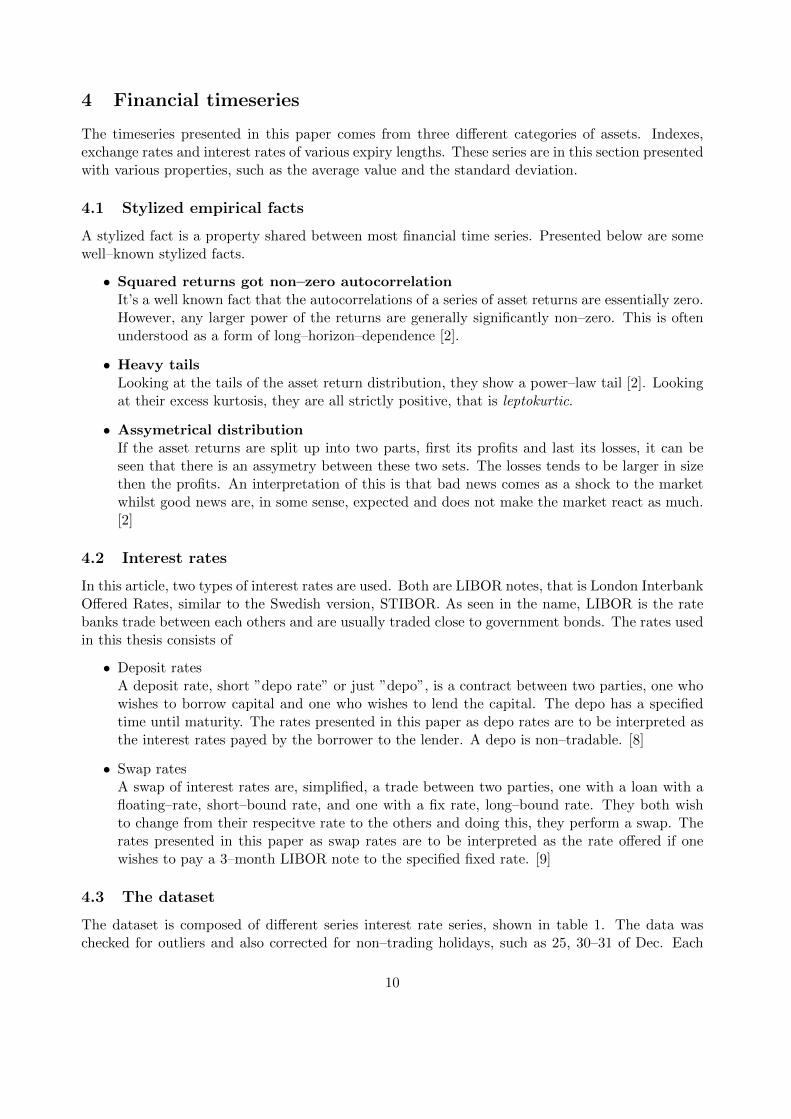
4 Financial timeseries

The timeseries presented in this paper comes from three different categories of assets. Indexes,exchange rates and interest rates of various expiry lengths. These series are in this section presentedwith various properties, such as the average value and the standard deviation.

4.1 Stylized empirical facts

A stylized fact is a property shared between most financial time series. Presented below are somewell–known stylized facts.

• Squared returns got non–zero autocorrelationIt’s a well known fact that the autocorrelations of a series of asset returns are essentially zero.However, any larger power of the returns are generally significantly non–zero. This is oftenunderstood as a form of long–horizon–dependence [2].

• Heavy tailsLooking at the tails of the asset return distribution, they show a power–law tail [2]. Lookingat their excess kurtosis, they are all strictly positive, that is leptokurtic.

• Assymetrical distributionIf the asset returns are split up into two parts, first its profits and last its losses, it can beseen that there is an assymetry between these two sets. The losses tends to be larger in sizethen the profits. An interpretation of this is that bad news comes as a shock to the marketwhilst good news are, in some sense, expected and does not make the market react as much.[2]

4.2 Interest rates

In this article, two types of interest rates are used. Both are LIBOR notes, that is London InterbankOffered Rates, similar to the Swedish version, STIBOR. As seen in the name, LIBOR is the ratebanks trade between each others and are usually traded close to government bonds. The rates usedin this thesis consists of

• Deposit ratesA deposit rate, short ”depo rate” or just ”depo”, is a contract between two parties, one whowishes to borrow capital and one who wishes to lend the capital. The depo has a specifiedtime until maturity. The rates presented in this paper as depo rates are to be interpreted asthe interest rates payed by the borrower to the lender. A depo is non–tradable. [8]

• Swap ratesA swap of interest rates are, simplified, a trade between two parties, one with a loan with afloating–rate, short–bound rate, and one with a fix rate, long–bound rate. They both wishto change from their respecitve rate to the others and doing this, they perform a swap. Therates presented in this paper as swap rates are to be interpreted as the rate offered if onewishes to pay a 3–month LIBOR note to the specified fixed rate. [9]

4.3 The dataset

The dataset is composed of different series interest rate series, shown in table 1. The data waschecked for outliers and also corrected for non–trading holidays, such as 25, 30–31 of Dec. Each

10

of these series span over the dates 2000-01-01 to 2011-01-01 if nothing else is specified. So calledHoliday effects are neglected in this thesis.

Name MaturityEUR LIBOR 3MEUR LIBOR 1YUSD LIBOR 3MUSD LIBOR 1Y

Table 1: Analyzed time series.

11

5 Implementation

The theory previously presented is used in computer programs, the code presented in appendix A.This section presents the algorithms and methods used to construct the tests.

5.1 Optimal block length

In calculations of the optimal block length by the VARJAB, Monte–Carlo–simulations are run toestimate value–at–risk for a time series. Doing so, many resamples are produced, but these arenot enough, subsampling through the jackknife method are also required. This is a very expensive,computation wise, procedure. However, through the use of following theorem a reuse of resamplesare allowed.

Theorem Let J1, . . . , Jb be iid discrete uniform random variables on {1, . . . , N} and let {Ji1, . . . , Jib}be iid discrete uniform random variables on Ii, see section 3.5, 1 ≤ i ≤M . Also, pi =

∑bj=1 1{Jj∈Ii}/b

Then P(J1 = j1, . . . , Jb = jb|pi = 1) = P(Ji1 = j1, . . . , Jib = jb).

That is, given that one resample misses the blocks indexed i, . . . , i + m − 1, the probability ofit having certain blocks is the same as it having the same blocks but not being able to choose fromthe missing blocks in the first place [7]. Thus the procedure of calculating the jackknife–after–bootstrap estimate och the variance is a matter of finding the resamples that already have a lackof the desired blocks.

First of, start by Monte–Carlo–simulating ϕn This is done by fixing a block length, `, and thensimulating K resamples, {kB∗1 , . . . , kB∗b }, k = 1, . . . ,K. These resamples are stored for future use.For each resample, take the 100(1−α)% worst multi–period event and call this your value–at–riskestimate. Finally take the sample mean of the estimates.

To measure VARJAB, ϕ(i)n is calculated by choosing the resamples, already calculated in the

Monte–Carlo–simulations, that lack blocks i, . . . , i + m − 1. That is choose the resamples where{kB∗1 , . . . , kB∗b } ∩ {Bi, . . . , Bi+m−1} = ∅. The suggested optimal block length is then gotten as insection 3.5.

5.2 VaR–estimaton by block bootstrap

To use the block bootstrap method to estimate the density function of the m day multiperiodreturns, m ≥ 1, from the daily return data {Xi}ni=1, we follow these simple instructions.

• Construct a set of blocks B` = {B`1, . . . , B

`n} where B`

i = {Xi, . . . , Xi+`}.

• Draw b discrete uniform random numbers from 1 to n, call them {Ui}bi=1.

• Choose b blocks from B` by taking the block with indexes Ui. That is, B`∗ = {B`

U1, . . . , B`

Ub} =

X∗ = {X∗1 , . . . , X∗n}.

• Compound the resample, {X∗1 + · · ·+Xm, . . . , Xn−m+1 + · · ·+X∗n}, m ≥ 1

• Sort X∗ by size, smallest first, and choose the nα first element, X∗(nα). Store this number.

• Repeat this procedure N times and after that take the sample mean of the observations. Thisis an estimate of the α–VaR.

12

5.3 VaR–estimation by stationary bootstrap

An algorithm for VaR estimation by the stationary bootstrap is presented with these step–by–stepinstructions.

Construct a set of numbers U = {U1, . . . , Un} by following these procedures. If at any time Ugot n elements, quit the algorithm.

• Set i to 1.

• Choose a number from a discrete uniform distribution over the numbers 1 to n. Store thisnumber as Ui.

• With probability p jump to the next step and with probability 1−p increase i by 1 and jumpto the previous step.

• Choose Ui+1 as Ui + 1, increase i by 1 and jump to the previous step.

Now construct a stationary bootstrap resample, X∗, by choosing the elements of X with indexes U .To get the m day VaR–estimate with level α, follow the procedures 4–5 from section 5.2. Repeatall of these procedures N times and after that, take the sample mean of these observations. Thisis the VaR–estimate.

5.4 Implementation of VaR backtest.

To construct a VaR backtest, a large historical data sample is needed. This is in practice a seriousproblem. When looking at the 99% level VaR for 10–days changes, one is essentially looking atthe worst event happening in 1000 days, i.e. roughly 4 years. To get a reasonable amount of datapoints for this risk measure in a back test many many years worth of data are needed.

There are also a problem with the choice of size of the data used for VaR estimation in thecalculations. Not enough data points and the model does not give an accurate estimate and toomany data points makes the risk measure to slow in capturing market changes. It is thus necessaryto make a compromise.

The construction of a backtest is a simple procedure but takes a considerable time to run. First of,split the data chosen for the backtest into two, not necessarily equal, parts. Think of the first partas the known history and consider the second part as if it had not already happened. The first partof the data is then used in the estimation of VaR, this estimate is then checked against the actualoutcome, from the second part of the data. Every time an actual outcome is worse than the VaRestimate, call this an exception, is counted and stored. Last, check if the number of exceptions issignificantly different from the α level suggested by the VaR model. If this is the case, the modelis not a good measure of VaR, at suggested significance level.

13

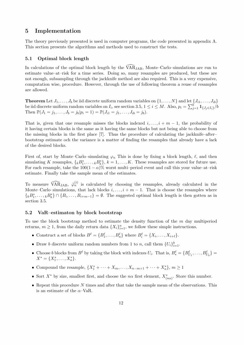
(a) Block length 1 (b) Block length 20 (c) Block length 40

Figure 1: Autocorrelation plots for resampled series (plus) with different block lengths and realdata (square).

6 Results

Now how well does these extended bootstrap versions replicate the properties of dependent timeseries? As seen in section 3.3, the block length is an unknown parameter and thus it might beinteresting to see how sensitive the distribution of returns estimates are for different block lengths.In this section, we will study the effects of an increasing block length on the tail of the distributionof varying multi–period returns. We will also perform backtests on time series to get a feel ifthese estimates are a good estimate of risk. Certain correctional techniques, such as weightingof more recent data and correlation with other time series, will be ignored mainly because of theassumptions that have to be done that risks to ”pollute” the data.

6.1 Choice of blocklength

Looking at the autocorrelation plots 1(a),1(b) and 1(c), there is a capture of autocorrelation up tothe lag equal to the block length in question. Thus, the VaR–measure seems to only care aboutcorrelation up to this point. Further on, looking at the sample variance for multi–period returns,figures 2,3,4, we see a clear deviation from a linear increase in the original sample. Also for theresampled data, the approximation of the variance for different multi–periods for the original seriesgets better as the block length increases.

As seen, there is a tendency to better and better describe the dependence structure the higherthe block length is and intuitively speaking, with a block length equal to the sample size, onewould expect to see the same autocorrelation structure as the original sample. The same reasoninggoes for the serial variance.

The empirical distribution function of the multi–period returns and the resampled data wascompared against each other through the K–S test, see figure 5. There is a clear trend in this datathat increasing block lengths up to the number of days in the multi–period returns lowers the K-Sdistance. As seen there is a local minimum when the block length equals the number of days inthe multi–period returns. The distribution fit is also illustrated in the QQ–plots shown in figures

14

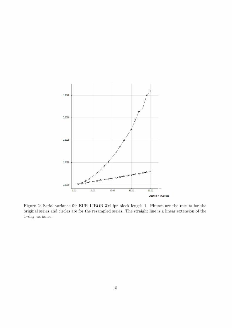
Figure 2: Serial variance for EUR LIBOR 3M fpr block length 1. Plusses are the results for theoriginal series and circles are for the resampled series. The straight line is a linear extension of the1–day variance.

15

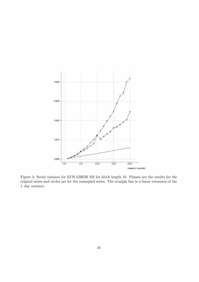
Figure 3: Serial variance for EUR LIBOR 3M for block length 10. Plusses are the results for theoriginal series and circles are for the resampled series. The straight line is a linear extension of the1–day variance.

16

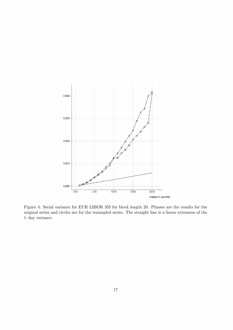
Figure 4: Serial variance for EUR LIBOR 3M for block length 20. Plusses are the results for theoriginal series and circles are for the resampled series. The straight line is a linear extension of the1–day variance.

17

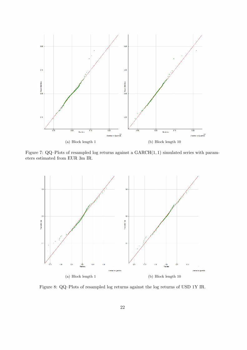
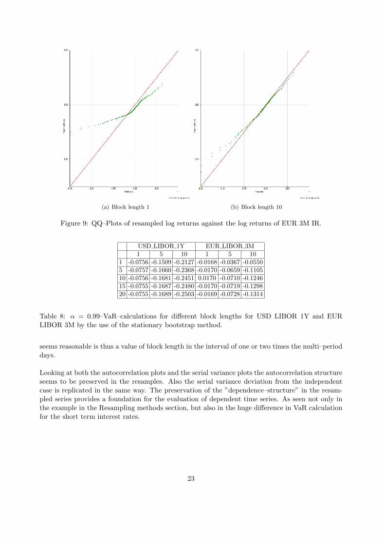
8 and 9.

Now shifting attention towards the tails of the distribution function of the multi–period returns,how do they behave as we increase the block length? In tables 5, 6, 7 and 8, the results of this testis presented. Looking at these tables, value–at–risk increases, in magnitude, quickly as the blocklength increases to the number of multi–period days in question and after this, reaching a plateau.This behaviour could be interpreted as the VaR–method requiring only the correlation structureup until the amount of multi–period days it is looking at.

These results would imply that one should choose a block length high enough to capture enoughof the autocorrelation structure and distribution function properties. However, since a large blocklength decreases the number of drawn blocks, the variance of the estimation would be expected toincrease, thus a method for calculating the optimal block length built on MSE minimization werealso considered.

The JAB method to estimate the optimal block length for different time series with differentmultiperiods and different levels of VaR. 100000 resamples were used in this process. The resultsare presented in tables 2 and 3 and shows similar results as the previous tests. As the multi–perioddays increases, the suggested block length increases as well at roughly the same size as the multi–period days.

SEK3M EUR3M USD1Y USD3M EUR1Y1 0.79 0.64 0.58 1.81 1.155 5.39 7.18 2.97 4.80 3.72

10 9.73 10.00 3.16 8.45 4.05

Table 2: Suggested block length by the JAB–method for different time series for various multi–period returns, α = 0.95.

SEK3M EUR3M USD1Y USD3M EUR1Y1 1.44 1.27 1.01 0.90 3.135 3.22 6.65 4.61 7.83 4.28

10 6.33 8.49 5.31 12.28 6.00

Table 3: Suggested block length by the JAB–method for different time series for various multi–period returns, α = 0.99.

6.2 Backtests

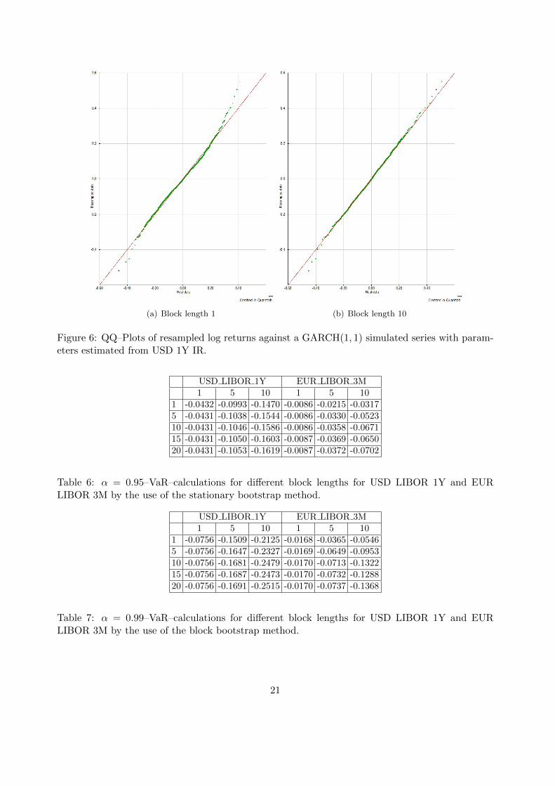
A GARCH(1, 1) process was used to create a large number of data. The parameters used were es-timated from the log returns of the 3 month EUR LIBOR note using a maximum likelihood basedsoftware. The initial volatility was estimated by the variance of the log returns of the time series.From these parameters, a new dataset was constructed by following the GARCH(1, 1) model andrecursively calculating the innovations at, as defined in section 2.7. The series produced was usedto check the fit of distributions by QQ–plots, as seen in figures 6 and 7.

18

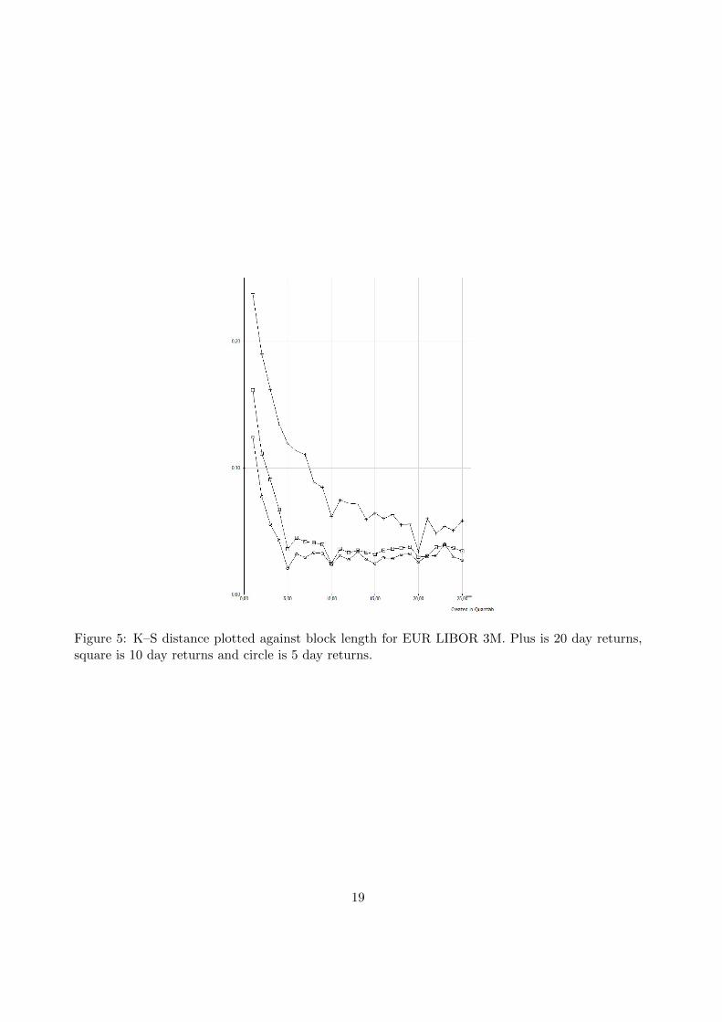
Figure 5: K–S distance plotted against block length for EUR LIBOR 3M. Plus is 20 day returns,square is 10 day returns and circle is 5 day returns.

19

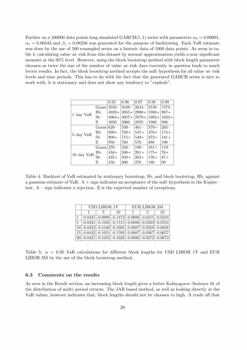
Further on a 100000 data points long simulated GARCH(1, 1) series with parameters α0 = 0.00001,α1 = 0.80443 and β1 = 0.08256 was generated for the purpose of backtesting. Each VaR estimatewas done by the use of 500 resampled series on a historic data of 1000 data points. As seem in ta-ble 4, calculating value–at–risk from this dataset by normal–approximation yields a non–significantmeasure at the 95% level. However, using the block bootstrap method with block length parameterchoosen as twice the size of the number of value–at–risk days currently in question leads to muchbetter results. In fact, the block bootstrap method accepts the null–hypothesis for all value–at–risklevels and time periods. This has to do with the fact that the generated GARCH series is nice towork with, it is stationary and does not show any tendency to ”explode”.

0.95 0.96 0.97 0.98 0.99

1–day VaR

Gauss 3550– 3108– 2644– 2138– 1573–Bb 4939+ 3955+ 2990+ 1988+ 987+Sb 4964+ 3957+ 2979+ 1992+ 1023+E 4950 3960 2970 1980 990

5–day VaR

Gauss 620– 530– 461– 379+ 265–Bb 939+ 728+ 547+ 370+ 174+Sb 908+ 715+ 549+ 372+ 181+E 950 760 570 380 190

10–day VaR

Gauss 276– 228– 199– 161+ 119–Bb 434+ 348+ 261+ 175+ 76+Sb 435+ 350+ 262+ 176+ 87+E 450 360 270 180 90

Table 4: Backtest of VaR estimated by stationary bootstrap, Sb, and block bootstrap, Bb, againsta gaussian estimate of VaR. A + sign indicates an acceptance of the null–hypothesis in the Kupiec–test. A – sign indicates a rejection. E is the expected number of exceptions.

USD LIBOR 1Y EUR LIBOR 3M1 5 10 1 5 10

1 -0.0431 -0.0995 -0.1472 -0.0086 -0.0215 -0.03165 -0.0431 -0.1035 -0.1515 -0.0086 -0.0333 -0.055410 -0.0432 -0.1046 -0.1605 -0.0087 -0.0358 -0.062615 -0.0432 -0.1051 -0.1593 -0.0087 -0.0367 -0.065720 -0.0431 -0.1053 -0.1628 -0.0086 -0.0372 -0.0673

Table 5: α = 0.95–VaR–calculations for different block lengths for USD LIBOR 1Y and EURLIBOR 3M by the use of the block bootstrap method.

6.3 Comments on the results

As seen in the Result section, an increasing block length gives a better Kolmogorov–Smirnov fit ofthe distribution of multi–period returns. The JAB based method, as well as looking directly at theVaR values, however indicates that, block lengths should not be choosen to high. A trade off that

20

(a) Block length 1 (b) Block length 10

Figure 6: QQ–Plots of resampled log returns against a GARCH(1, 1) simulated series with param-eters estimated from USD 1Y IR.


1 -0.0432 -0.0993 -0.1470 -0.0086 -0.0215 -0.03175 -0.0431 -0.1038 -0.1544 -0.0086 -0.0330 -0.052310 -0.0431 -0.1046 -0.1586 -0.0086 -0.0358 -0.067115 -0.0431 -0.1050 -0.1603 -0.0087 -0.0369 -0.065020 -0.0431 -0.1053 -0.1619 -0.0087 -0.0372 -0.0702

Table 6: α = 0.95–VaR–calculations for different block lengths for USD LIBOR 1Y and EURLIBOR 3M by the use of the stationary bootstrap method.


1 -0.0756 -0.1509 -0.2125 -0.0168 -0.0365 -0.05465 -0.0756 -0.1647 -0.2327 -0.0169 -0.0649 -0.095310 -0.0756 -0.1681 -0.2479 -0.0170 -0.0713 -0.132215 -0.0756 -0.1687 -0.2473 -0.0170 -0.0732 -0.128820 -0.0756 -0.1691 -0.2515 -0.0170 -0.0737 -0.1368

Table 7: α = 0.99–VaR–calculations for different block lengths for USD LIBOR 1Y and EURLIBOR 3M by the use of the block bootstrap method.

21


Figure 7: QQ–Plots of resampled log returns against a GARCH(1, 1) simulated series with param-eters estimated from EUR 3m IR.


Figure 8: QQ–Plots of resampled log returns against the log returns of USD 1Y IR.

22


Figure 9: QQ–Plots of resampled log returns against the log returns of EUR 3M IR.


1 -0.0756 -0.1509 -0.2127 -0.0168 -0.0367 -0.05505 -0.0757 -0.1660 -0.2368 -0.0170 -0.0659 -0.110510 -0.0756 -0.1681 -0.2451 0.0170 -0.0710 -0.124615 -0.0755 -0.1687 -0.2480 -0.0170 -0.0719 -0.129820 -0.0755 -0.1689 -0.2503 -0.0169 -0.0728 -0.1314

Table 8: α = 0.99–VaR–calculations for different block lengths for USD LIBOR 1Y and EURLIBOR 3M by the use of the stationary bootstrap method.

seems reasonable is thus a value of block length in the interval of one or two times the multi–perioddays.

Looking at both the autocorrelation plots and the serial variance plots the autocorrelation structureseems to be preserved in the resamples. Also the serial variance deviation from the independentcase is replicated in the same way. The preservation of the ”dependence–structure” in the resam-pled series provides a foundation for the evaluation of dependent time series. As seen not only inthe example in the Resampling methods section, but also in the huge difference in VaR calculationfor the short term interest rates.

23

References

[1] Patrik Albin. Lecture notes in the course ”stochastic data processing and simulation”. Avail-able at http://www.math.chalmers.se/Stat/Grundutb/CTH/tms150/1011, 2011–08–17.

[2] Rama Cont. Empirical properties of asset returns: stylized facts and statistical issues. Quan-titative Finance, 1:223–236, 2001.

[3] Bradley Efron. Bootstrap methods: Another look at the jackknife. The Annals of Statistics,7(1):1–26, 1979.

[4] LLC Eola Investments. Notes on the bootstrap mehod. Available at http://

eolainvestments.com/Documents/Notes%20on%20The%20Bootstrap%20Method.pdf, 2011–06–13.

[5] Paul H. Kupiec. Techniques for verifying the accuracy of risk measurement models. TheJournal of Derivatives, 3(2):73–84, 1995.

[6] S.N. Lahiri. On the jackknife after bootstrap method for dependent data and its consistencyproperties. Econometric Theory, 18:79–98, 2002.

[7] S.N. Lahiri. Resampling Methods for Dependent Data. Springer–Verlag New York, Inc, 2010.

[8] Johan A Lybeck and Gustaf Hagerud. Penningmarknadens Instrument. Raben & Sjogren,1988.

[9] Lionel Martellini, Philippe Priaulet, and Stephane Priaulet. Fixed–Income Securities. JohnWiley & Sons, Inc., 2003.

[10] Daniel J. Nordman. A note on the stationary bootstrap’s variance. The Annals of Statistics,37(1):359–370, 2009.

[11] Dimitris N. Politis and Joseph P. Romano. The stationary bootstrap. Technical Report 91–03,Purdue University, 1991.

[12] Ruey S. Tsay. Analysis of Financial Time Series. John Wiley & Sons, Inc., Hoboken, NewJersey, 3rd edition, 2010.

A C#–code

The programs used in calculations in this thesis are The basic building blocks are presented here.

class Norm

{

private WH2006 _myRand = new WH2006();

//Normal-dist r.v. generator using Box-Muller

public double Rnd(double mu, double sigma)

{

double chi = _myRand.NextDouble();

double eta = _myRand.NextDouble();

double z = mu + sigma * Math.Sqrt(-2 * Math.Log(chi)) * Math.Cos(2 * Math.PI * eta);

return z;

}

public static double N(double x)

{

const double b1 = 0.319381530;

const double b2 = -0.356563782;


const double b4 = -1.821255978;


const double p = 0.2316419;

const double c = 0.39894228;

if (x >= 0.0)

{

double t = 1.0 / (1.0 + p * x);

return (1.0 - c * Math.Exp(-x * x / 2.0) * t *

(t * (t * (t * (t * b5 + b4) + b3) + b2) + b1));

}

else

{

double t = 1.0 / (1.0 - p * x);

return (c * Math.Exp(-x * x / 2.0) * t *

(t * (t * (t * (t * b5 + b4) + b3) + b2) + b1));

}

}

public static double InvN(double alpha)

{

double eps = 0.00000001;

int counter = 0;

double guess = 10;

bool nonconv = true;

if (alpha < 0.5)

{

25

guess = -1.0*InvN(1 - alpha);

}

else

{

while(counter<100000 && nonconv )

{

double inv = N(guess);

if (Math.Abs(inv - alpha) > eps)

{

int sign = Math.Sign(alpha-inv);

guess = guess + sign*10.0/Math.Pow(2.0,counter+1);

counter++;

}

else

{

nonconv = false;

}

}

guess = nonconv ? -100000.0 : guess;

}

return guess;

}

}

class DataBase

{

//Static Instance Method

public static List<string> Name()

{

List<string> data = new List<string>();

SqlConnection myConnection = new SqlConnection("user id=’’;" +

"password=’’;server=tambora;" +

"Trusted_Connection=yes;" +

"database=arms_yahoo; " +

"connection timeout=30");

try

{

myConnection.Open();

}

catch (Exception e)

{

Console.WriteLine(e.ToString());

}

try

{

26

SqlDataReader myReader = null;

string sql_q =

"SELECT item FROM ahs_data_float WHERE item NOT LIKE ’%_OLD’ GROUP BY item ";

SqlCommand myCommand = new SqlCommand(sql_q, myConnection);

myReader = myCommand.ExecuteReader();

while (myReader.Read())

{

data.Add(myReader.GetString(0));

}

}

catch (Exception e)

{


}

try

{

myConnection.Close();

}

catch (Exception e)

{


}

return data;

}

//Instance Method

public List<double> Get(string series)

{

List<double> data = new List<double>();






try

{


}

catch (Exception e)

{


}

try

{


string sql_q =

"SELECT val FROM ahs_data_float WHERE item = @Param1 AND"

+"(quote_date BETWEEN ’2000-01-01’ AND ’2011-01-01’) ORDER BY quote_date";

27

SqlParameter myParam = new SqlParameter("@Param1", SqlDbType.VarChar);

myParam.Value = series;


myCommand.Parameters.Add(myParam);



{

data.Add(myReader.GetDouble(0));

}

}

catch (Exception e)

{


}

try

{


}

catch (Exception e)

{


}

return data;

}

public List<double> GetFull(string series)

{

List<double> data = new List<double>();






try

{


}

catch (Exception e)

{


}

try

{


// AND (quote_date BETWEEN ’2000-01-01’ AND ’2011-01-01’)

string sql_q =

"SELECT val FROM ahs_data_float WHERE item = @Param1 ORDER BY quote_date";

SqlParameter myParam = new SqlParameter("@Param1", SqlDbType.VarChar);

28

myParam.Value = series;


myCommand.Parameters.Add(myParam);



{

data.Add(myReader.GetDouble(0));

}

}

catch (Exception e)

{


}

try

{


}

catch (Exception e)

{


}

return data;

}

//Destructor

// ~DataBase()

// {

// Some resource cleanup routines.

// }

}

class Resampler

{

//Block length: 1 is 1 data point, 2 is 2 data points and so on..

private List<double> _data = new List<double>();

private int _blockLength = 0;

private int _lData = 0;

WH2006 _myRand;

public Resampler(int blockLength,List<double> data)

{

_blockLength = blockLength;

_data = data;

_lData = _data.Count();

_myRand = new WH2006();

}

public List<double> GetResample()

{

//Init. random nr.

29

//SystemCryptoRandomNumberGenerator myRand = new SystemCryptoRandomNumberGenerator();

List<double> resample = new List<double>();

//Draw a starting point in the data.

int m = _myRand.Next(_lData);

for(int i=0;i<_lData;i++)

{

//Generate either a random nr m: 0<=m<=_lData-1 or increase

//m by 1 depending on the block length.

m = ((i+1)%_blockLength != 0) ? m+1:_myRand.Next(_lData);

//Choose the cyclic (m%_ldata) element, 0<=m<=_ldata+_blockLength-1,

//to add to resample.

resample.Add(_data[m%_lData]);

}

return resample;

}

}

class Bb

{


private double _alpha;

private int _blockLength;

private int _varDays;

private int _lData;

public Bb(double alpha,List<double> data,int blockLength,int varDays)

{

_alpha = alpha;

_data = data;


_varDays = varDays;


}

private double LinInterpolVaR(List<double> sample)

{

sample.Sort();

int lSample = sample.Count();

double alphaInd = (1 - _alpha) * (lSample - 1);

double lower = Math.Floor(alphaInd);

double x = alphaInd - lower;

double upper = Math.Ceiling(alphaInd);

double uVal = sample[(int)upper];

double lVal = sample[(int)lower];

return lVal + x * (uVal - lVal);

}

private double VaR(List<double> sample)

30

{

sample.Sort();


int alphaInd = (int)Math.Floor((1 - _alpha) * (lSample - 1));

return sample[alphaInd];

}

private double Pfe(List<double> sample)

{

sample.Sort();


int alphaInd = (int)Math.Ceiling(_alpha * (lSample-1));


}

private List<double> CompData(List<double> sample)

{


List<double> compData = new List<double>();

int nl = lSample/_varDays;

for (int i = 0; i < lSample; i++)

{

if (i >= nl)

{

int k = i%nl;

int j = i/nl;

compData[k] += sample[k*_varDays+j];

}

else

{

compData.Add(sample[i*_varDays]);

}

}

return compData;

}

public double GetVaR(int numSim)

{

double varEst = 0.0;

Resampler myResampler = new Resampler(_blockLength, _data);

for (int i = 0; i < numSim; i++)

{

List<double> resample = myResampler.GetResample();

List<double> compData = CompData(resample);

varEst+=VaR(compData);

}

return varEst*1.0/numSim;

}

public double GetUpperVaR(int numSim, double confInv)

{

31

List<double> varEst = new List<double>();



{



varEst.Add(VaR(compData));

}

varEst.Sort();

int confInd = (int)Math.Ceiling(((numSim - 1) * confInv));

return varEst[confInd];

}

public double GetLowerVaR(int numSim, double confInv)

{

List<double> varEst = new List<double>();



{



varEst.Add(VaR(compData));

}

varEst.Sort();

int confInd = (int)((numSim - 1) * (1-confInv));

return varEst[confInd];

}

public double GetLinInterpolVaR(int numSim)

{

double varEst = 0.0;



{



varEst += LinInterpolVaR(compData);

}

return varEst * 1.0 / numSim;

}

public double GetPfe(int numSim)

{

double pfeEst = 0.0;



{


pfeEst += Pfe(CompData(resample));

}

32

return pfeEst * 1.0 / numSim;

}

}

class BackTest

{





private int _lData;

private int _numSim;

public BackTest(List<double> data,int varDays,int blockLenght,double alpha,int numSim)

{

_numSim = numSim;

_data = data;

_varDays = varDays;


_blockLength = blockLenght;

_alpha = alpha;

}

static double Variance(List<double> data)

{

double mean = data.Average();

int size = data.Count();

double var = 0.0;

for (int i = 0; i < size; i++)

{

var += Math.Pow(data[i] - mean, 2.0);

}

return var / (size - 1);

}


{



int nl = lSample / _varDays;


{

if (i >= nl)

{

int k = i % nl;

int j = i / nl;

compData[k] += sample[k * _varDays + j];

}

else

{

compData.Add(sample[i]);

33

}

}

return compData;

}

private static List<double> SubVector(List<double> data,

int indStart,int numberOfElements)

{

List<double> subVector = new List<double>();

for (int i = indStart; i < indStart+numberOfElements; i++)

{

subVector.Add(data[i]);

}

return subVector;

}


{

sample.Sort();




}

private double Pfe(List<double> sample)

{

sample.Sort();


int alphaInd = (int)Math.Ceiling(_alpha * (lSample - 1));


}

public int NoExceptions(int lHistoric)

{

int lFuture = _lData - lHistoric;

int noChecks = lFuture/_varDays;

int exceptions = 0;

for(int i=0;i<noChecks;i++)

{

List<double> sample = SubVector(_data, i*_varDays, lHistoric);

Bb myBb = new Bb(_alpha, sample, _blockLength, _varDays);

double varEst = myBb.GetVaR(_numSim);

double future = SubVector(_data,lHistoric+i*_varDays,_varDays).Sum();

if(future<varEst)

{

exceptions++;

}

}

return exceptions;

}

public int NoExceptionsPfe(int lHistoric)

34

{


int noChecks = lFuture / _varDays;

int exceptions = 0;

for (int i = 0; i < noChecks; i++)

{

List<double> sample = SubVector(_data, i * _varDays, lHistoric);


double pfeEst = myBb.GetPfe(_numSim);

double future = SubVector(_data, lHistoric + i * _varDays, _varDays).Sum();

if (future > pfeEst)

{

exceptions++;

}

}

return exceptions;

}

public int NoExceptionsConf(int lHistoric,double confLvl,string method)

{

if (method == "upper")

{



int exceptions = 0;


{



double varEst = myBb.GetUpperVaR(_numSim,confLvl);


if (future < varEst)

{

exceptions++;

}

}

return exceptions;

}

else

{



int exceptions = 0;


{



35

double varEst = myBb.GetLowerVaR(_numSim,confLvl);


if (future < varEst)

{

exceptions++;

}

}

return exceptions;

}

}

public int NoExceptionsPfeConf(int lHistoric, double confLvl, string method)

{



int exceptions = 0;


{



double pfeEst = myBb.GetPfe(_numSim);


if (future > pfeEst)

{

exceptions++;

}

}

return exceptions;

}

public int NoExceptionsGaussVaR(int lHistoric)

{


int noChecks = lFuture/_varDays;

int exceptions = 0;

double z = Norm.InvN((1-_alpha));

double sqrtVarDay = Math.Sqrt(_varDays);

for (int i = 0; i < noChecks - 1; i++)

{


double mu = sample.Average();

double s = Math.Sqrt(Variance(sample));

double var = sqrtVarDay * s * z;


if (future < var)

{

exceptions++;

}

36

}

return exceptions;

}

public int NoExceptionsGaussPfe(int lHistoric)

{



int exceptions = 0;

double z = Norm.InvN((_alpha));

double sqrtVarDay = Math.Sqrt(_varDays);


{


double mu = sample.Average();

double s = Math.Sqrt(Variance(sample));

double pfe = sqrtVarDay* s * z;


if (future > pfe)

{

exceptions++;

}

}

return exceptions;

}

public int NoExceptionsHistVaR(int lHistoric)

{


int exceptions = 0;


for (int i = 0; i < noChecks-1; i++)

{


double var = VaR(sample);


if (future < var)

{

exceptions++;

}

}

return exceptions;

}

public int NoExceptionsHistPfe(int lHistoric)

{


int exceptions = 0;



37

{


double pfe = Pfe(sample);


if (future > pfe)

{

exceptions++;

}

}

return exceptions;

}

}

class Blocks

{


private int _lData;


private List<List<double>> _blocks = new List<List<double>>();

public Blocks(List<double> data,int blockLength)

{

_data = data;



if (_blockLength < 1)

{

_blockLength = 1;

}

else if (_blockLength > _lData)

{

_blockLength = _lData;

}

}

public void CreateBlocks()

{

// Creates the matrix, _blocks, containing the blocks.

// this.Get(n) gets the n:th block.

for (int i = 0; i < _lData; i++)

{

List<double> blockTemp = new List<double>();

for (int j = 0; j < _blockLength; j++)

{

blockTemp.Add(_data[(i+j)%_lData]);

}

_blocks.Add(blockTemp);

}

38

}

public List<double> Get(int n)

{

// Gets the block of length blockLength starting at index n.

// Must run this.CreateBlocks() first.

return _blocks[n];

}

}

class Jab

{


private WH2006 _myRand = new WH2006();


private int _lData;

private int _noBlocks;

private int _numberOfSimulations;

private List<List<int>> _indexes = new List<List<int>>();

private Blocks _myBlock;


private int _blockOfBlocks;


public Jab(List<double> data, int blockLength,

int numberOfSimulations,double alpha,int blockOfBlocks,int varDays)

{

_data = data;


_blockLength = blockLength > 0 ? blockLength:1;

_noBlocks = _lData / _blockLength;

_numberOfSimulations = numberOfSimulations;

IndexCreator();

_myBlock = new Blocks(_data, _blockLength);

_myBlock.CreateBlocks();

_alpha = alpha;

_blockOfBlocks = blockOfBlocks;

_varDays = varDays;

}


{



int nl = lSample / _varDays;


{

if (i >= nl)

{

int k = i % nl;

int j = i / nl;

39

compData[k] += sample[k * _varDays + j];

}

else

{

compData.Add(sample[i * _varDays]);

}

}

return compData;

}

private void IndexCreator()

{

for (int i = 0; i < _numberOfSimulations; i++)

{

List<int> tempInd = new List<int>();

for (int j = 0; j < _noBlocks; j++)

{

tempInd.Add(_myRand.Next(_lData));

}

_indexes.Add(tempInd);

}

}

private List<double> Resampler(List<int> indexVector)

{

List<double> resampledData = new List<double>();

foreach (int ind in indexVector)

{

resampledData.AddRange(_myBlock.Get(ind));

}

return resampledData;

}


{

sample.Sort();




}

public double MonteCarlo()

{

double mc = 0.0;


{

mc += VaR(CompData(Resampler(_indexes[i])));

}

return mc/_numberOfSimulations;

}

private bool IsEmpty(int blockNr, int start)

40

{

List<int> setBlocks = new List<int>();

for (int i = start; i < start + _blockOfBlocks; i++)

{

setBlocks.Add(i);

}

IEnumerable<int> disjoint = _indexes[blockNr].Intersect(setBlocks);

int j = 0;

foreach (int d in disjoint)

{

j++;

}

return j==0?true:false;

}

public double Phi_i(int index)

{

int noSim = 0;

double var = 0.0;


{

if (IsEmpty(i, index))

{

noSim++;

var += VaR(CompData(Resampler(_indexes[i])));

}

}

return var/noSim;

}

public double Mse()

{

int M = _noBlocks - _blockOfBlocks+1;

int N = _lData - _blockLength + 1;

int n = _lData;

double mse = 0.0;

double phi = MonteCarlo();

for (int i = 0; i < M; i++)

{

double phi_i = Phi_i(i);

double temp = (phi *N - (N - _blockOfBlocks) * phi_i) / _blockOfBlocks;

mse += temp*temp;

}

return mse * (double)_blockOfBlocks / (M*(N - _blockOfBlocks));

}

}

41

Bootstrap of Dependent Data in Finance - Chalmerspalbin/BootstrapDependentAndreasSunesson.pdf ·...

Documents

Transcript of Bootstrap of Dependent Data in Finance - Chalmerspalbin/BootstrapDependentAndreasSunesson.pdf ·...