Boosting the Margin: A New Explanation for the …rob.schapire.net/papers/SchapireFrBaLe98.pdfA New...
30
The Annals of Statistics, 26(5):1651-1686, 1998. Boosting the Margin: A New Explanation for the Effectiveness of Voting Methods Robert E. Schapire AT&T Labs 180 Park Avenue, Room A279 Florham Park, NJ 07932-0971 USA [email protected] Yoav Freund AT&T Labs 180 Park Avenue, Room A205 Florham Park, NJ 07932-0971 USA [email protected] Peter Bartlett Dept. of Systems Engineering RSISE, Aust. National University Canberra, ACT 0200 Australia [email protected] Wee Sun Lee School of Electrical Engineering University College UNSW Australian Defence Force Academy Canberra ACT 2600 Australia [email protected] May 7, 1998 Abstract. One of the surprising recurring phenomena observed in experiments with boosting is that the test error of the generated classifier usually does not increase as its size becomes very large, and often is observed to decrease even after the training error reaches zero. In this paper, we show that this phenomenon is related to the distribution of margins of the training examples with respect to the generated voting classification rule, where the margin of an example is simply the difference between the number of correct votes and the maximum number of votes received by any incorrect label. We show that techniques used in the analysis of Vapnik’s support vector classifiers and of neural networks with small weights can be applied to voting methods to relate the margin distribution to the test error. We also show theoretically and experimentally that boosting is especially effective at increasing the margins of the training examples. Finally, we compare our explanation to those based on the bias-variance decomposition. 1 Introduction This paper is about methods for improving the performance of a learning algorithm, sometimes also called a prediction algorithm or classification method. Such an algorithm operates on a given set of instances (or cases) to produce a classifier, sometimes also called a classification rule or, in the machine-learning literature, a hypothesis. The goal of a learning algorithm is to find a classifier with low generalization or prediction error, i.e., a low misclassification rate on a separate test set. In recent years, there has been growing interest in learning algorithms which achieve high accuracy by voting the predictions of several classifiers. For example, several researchers have reported significant improvements in performance using voting methods with decision-tree learning algorithms such as C4.5 or CART as well as with neural networks [3, 6, 8, 12, 13, 16, 18, 29, 31, 37]. We refer to each of the classifiers that is combined in the vote as a base classifier and to the final voted classifier as the combined classifier. As examples of the effectiveness of these methods, consider the results of the following two experiments using the “letter” dataset. (All datasets are described in Appendix B.) In the first experiment, 1
Transcript of Boosting the Margin: A New Explanation for the …rob.schapire.net/papers/SchapireFrBaLe98.pdfA New...

The Annals of Statistics, 26(5):1651-1686, 1998.
Boosting the Margin:A New Explanation for the Effectiveness of Voting Methods
Robert E. SchapireAT&T Labs
180 Park Avenue, Room A279Florham Park, NJ 07932-0971 USA
Yoav FreundAT&T Labs
180 Park Avenue, Room A205Florham Park, NJ 07932-0971 USA
Peter BartlettDept. of Systems Engineering
RSISE, Aust. National UniversityCanberra, ACT 0200 Australia
Wee Sun LeeSchool of Electrical Engineering
University College UNSWAustralian Defence Force Academy
Canberra ACT 2600 [email protected]
May 7, 1998
Abstract. One of the surprising recurring phenomena observed in experiments with boosting is thatthe test error of the generated classifier usually does not increase as its size becomes very large, andoften is observed to decrease even after the training error reaches zero. In this paper, we show thatthis phenomenon is related to the distribution of margins of the training examples with respect to thegenerated voting classification rule, where the margin of an example is simply the difference betweenthe number of correct votes and the maximum number of votes received by any incorrect label. We showthat techniques used in the analysis of Vapnik’s support vector classifiers and of neural networks withsmall weights can be applied to voting methods to relate the margin distribution to the test error. Wealso show theoretically and experimentally that boosting is especially effective at increasing the marginsof the training examples. Finally, we compare our explanation to those based on the bias-variancedecomposition.
1 Introduction
This paper is about methods for improving the performance of a learning algorithm, sometimes alsocalled a prediction algorithm or classification method. Such an algorithm operates on a given setof instances (or cases) to produce a classifier, sometimes also called a classification rule or, in themachine-learning literature, a hypothesis. The goal of a learning algorithm is to find a classifier withlow generalization or prediction error, i.e., a low misclassification rate on a separate test set.
In recent years, there has been growing interest in learning algorithms which achieve high accuracyby voting the predictions of several classifiers. For example, several researchers have reported significantimprovements in performance using voting methods with decision-tree learning algorithms such as C4.5or CART as well as with neural networks [3, 6, 8, 12, 13, 16, 18, 29, 31, 37].
We refer to each of the classifiers that is combined in the vote as a base classifier and to the finalvoted classifier as the combined classifier.
As examples of the effectiveness of these methods, consider the results of the following twoexperiments using the “letter” dataset. (All datasets are described in Appendix B.) In the first experiment,
1

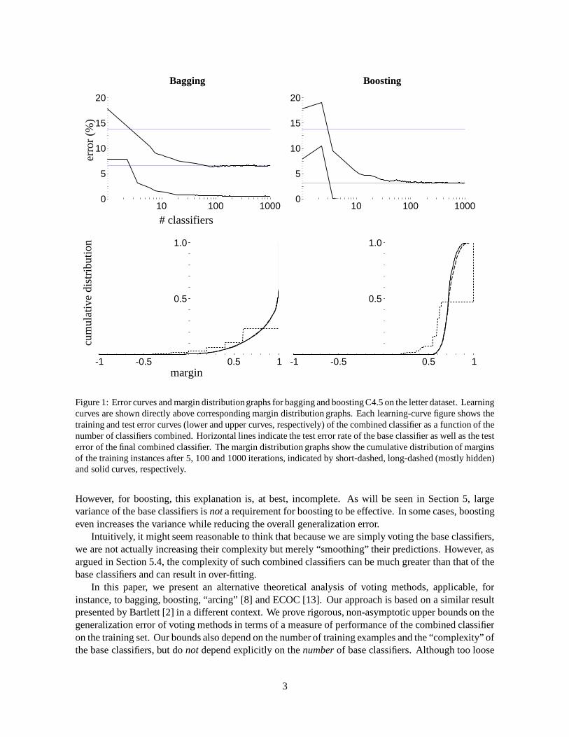
we used Breiman’s bagging method [6] on top of C4.5 [32], a decision-tree learning algorithm similarto CART [9]. That is, we reran C4.5 many times on random “bootstrap” subsamples and combined thecomputed trees using simple voting. In the top left of Figure 1, we have shown the training and test errorcurves (lower and upper curves, respectively) of the combined classifier as a function of the number oftrees combined. The test error of C4.5 on this dataset (run just once) is 13.8%. The test error of bagging1000 trees is 6.6%, a significant improvement. (Both of these error rates are indicated in the figure ashorizontal grid lines.)
In the second experiment, we used Freund and Schapire’s AdaBoost algorithm [20] on the samedataset, also using C4.5. This method is similar to bagging in that it reruns the base learning algorithmC4.5 many times and combines the computed trees using voting. However, the subsamples that are usedfor training each tree are chosen in a manner which concentrates on the “hardest” examples. (Detailsare given in Section 3.) The results of this experiment are shown in the top right of Figure 1. Note thatboosting drives the test error down even further to just 3.1%. Similar improvements in test error havebeen demonstrated on many other benchmark problems (see Figure 2).
These error curves reveal a remarkable phenomenon, first observed by Drucker and Cortes [16], andlater by Quinlan [31] and Breiman [8]. Ordinarily, as classifiers become more and more complex, weexpect their generalization error eventually to degrade. Yet these curves reveal that test error does notincrease for either method even after 1000 trees have been combined (by which point, the combinedclassifier involves more than two million decision-tree nodes). How can it be that such complexclassifiers have such low error rates? This seems especially surprising for boosting in which each newdecision tree is trained on an ever more specialized subsample of the training set.
Another apparent paradox is revealed in the error curve for AdaBoost. After just five trees havebeen combined, the training error of the combined classifier has already dropped to zero, but the testerror continues to drop1 from 8.4% on round 5 down to 3.1% on round 1000. Surely, a combinationof five trees is much simpler than a combination of 1000 trees, and both perform equally well on thetraining set (perfectly, in fact). So how can it be that the larger and more complex combined classifierperforms so much better on the test set?
The results of these experiments seem to contradict Occam’s razor, one of the fundamental principlesin the theory of machine learning. This principle states that in order to achieve good test error, theclassifier should be as simple as possible. By “simple,” we mean that the classifier is chosen froma restricted space of classifiers. When the space is finite, we use its cardinality as the measure ofcomplexity and when it is infinite we use the VC dimension [42] which is often closely related to thenumber of parameters that define the classifier. Typically, both in theory and in practice, the differencebetween the training error and the test error increases when the complexity of the classifier increases.
Indeed, such an analysis of boosting (which could also be applied to bagging) was carried out byFreund and Schapire [20] using the methods of Baum and Haussler [4]. This analysis predicts thatthe test error eventually will increase as the number of base classifiers combined increases. Such aprediction is clearly incorrect in the case of the experiments described above, as was pointed out byQuinlan [31] and Breiman [8]. The apparent contradiction is especially stark in the boosting experimentin which the test error continues to decrease even after the training error has reached zero.
Breiman [8] and others have proposed definitions of bias and variance for classification, and haveargued that voting methods work primarily by reducing the variance of a learning algorithm. Thisexplanation is useful for bagging in that bagging tends to be most effective when the variance is large.
1Even when the training error of the combined classifier reaches zero, AdaBoost continues to obtain new base classifiersby training the base learning algorithm on different subsamples of the data. Thus, the combined classifier continues to evolve,even after its training error reaches zero. See Section 3 for more detail.
2
Bagging Boostinger
ror
(%)
10 100 10000
5
10
15
20
10 100 10000
5
10
15
20
# classifiers
cum
ulat
ive
dist
ribu
tion
-1 -0.5 0.5 1
0.5
1.0
-1 -0.5 0.5 1
0.5
1.0
margin
Figure 1: Error curves and margin distributiongraphs for bagging and boosting C4.5 on the letter dataset. Learningcurves are shown directly above corresponding margin distribution graphs. Each learning-curve figure shows thetraining and test error curves (lower and upper curves, respectively) of the combined classifier as a function of thenumber of classifiers combined. Horizontal lines indicate the test error rate of the base classifier as well as the testerror of the final combined classifier. The margin distribution graphs show the cumulative distribution of marginsof the training instances after 5, 100 and 1000 iterations, indicated by short-dashed, long-dashed (mostly hidden)and solid curves, respectively.
However, for boosting, this explanation is, at best, incomplete. As will be seen in Section 5, largevariance of the base classifiers is not a requirement for boosting to be effective. In some cases, boostingeven increases the variance while reducing the overall generalization error.
Intuitively, it might seem reasonable to think that because we are simply voting the base classifiers,we are not actually increasing their complexity but merely “smoothing” their predictions. However, asargued in Section 5.4, the complexity of such combined classifiers can be much greater than that of thebase classifiers and can result in over-fitting.
In this paper, we present an alternative theoretical analysis of voting methods, applicable, forinstance, to bagging, boosting, “arcing” [8] and ECOC [13]. Our approach is based on a similar resultpresented by Bartlett [2] in a different context. We prove rigorous, non-asymptotic upper bounds on thegeneralization error of voting methods in terms of a measure of performance of the combined classifieron the training set. Our bounds also depend on the number of training examples and the “complexity” ofthe base classifiers, but do not depend explicitly on the number of base classifiers. Although too loose
3

0 5 10 15 20 25 30
bagging C4.5
0
5
10
15
20
25
30C
4.5
0 5 10 15 20 25 30
boosting C4.5
0
5
10
15
20
25
30
Figure 2: Comparison of C4.5 versus bagging C4.5 and boosting C4.5 on a set of 27 benchmark problems asreported by Freund and Schapire [18]. Each point in each scatter plot shows the test error rate of the two competingalgorithms on a single benchmark. The y-coordinate of each point gives the test error rate (in percent) of C4.5 onthe given benchmark, and the x-coordinate gives the error rate of bagging (left plot) or boosting (right plot). Allerror rates have been averaged over multiple runs.
to give practical quantitative predictions, our bounds do give a qualitative explanation of the shape ofthe observed learning curves, and our analysis may be helpful in understanding why these algorithmsfail or succeed, possibly leading to the design of even more effective voting methods.
The key idea of this analysis is the following. In order to analyze the generalization error, one shouldconsider more than just the training error, i.e., the number of incorrect classifications in the trainingset. One should also take into account the confidence of the classifications. Here, we use a measureof the classification confidence for which it is possible to prove that an improvement in this measureof confidence on the training set guarantees an improvement in the upper bound on the generalizationerror.
Consider a combined classifier whose prediction is the result of a vote (or a weighted vote) over a setof base classifiers. Suppose that the weights assigned to the different base classifiers are normalized sothat they sum to one. Fixing our attention on a particular example, we refer to the sum of the weights ofthe base classifiers that predict a particular label as the weight of that label. We define the classificationmargin for the example as the difference between the weight assigned to the correct label and themaximal weight assigned to any single incorrect label. It is easy to see that the margin is a number inthe range [�1; 1] and that an example is classified correctly if and only if its margin is positive. A largepositive margin can be interpreted as a “confident” correct classification.
Now consider the distribution of the margin over the whole set of training examples. To visualizethis distribution, we plot the fraction of examples whose margin is at most x as a function of x 2 [�1; 1].We refer to these graphs as margin distribution graphs. At the bottom of Figure 1, we show the margindistribution graphs that correspond to the experiments described above.
Our main observation is that both boosting and bagging tend to increase the margins associated with
4
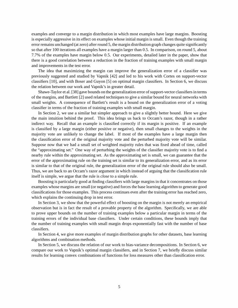
examples and converge to a margin distribution in which most examples have large margins. Boostingis especially aggressive in its effect on examples whose initial margin is small. Even though the trainingerror remains unchanged (at zero) after round 5, the margin distribution graph changes quite significantlyso that after 100 iterations all examples have a margin larger than 0.5. In comparison, on round 5, about7.7% of the examples have margin below 0:5. Our experiments, detailed later in the paper, show thatthere is a good correlation between a reduction in the fraction of training examples with small marginand improvements in the test error.
The idea that maximizing the margin can improve the generalization error of a classifier waspreviously suggested and studied by Vapnik [42] and led to his work with Cortes on support-vectorclassifiers [10], and with Boser and Guyon [5] on optimal margin classifiers. In Section 6, we discussthe relation between our work and Vapnik’s in greater detail.
Shawe-Taylor et al. [38] gave bounds on the generalization error of support-vector classifiers in termsof the margins, and Bartlett [2] used related techniques to give a similar bound for neural networks withsmall weights. A consequence of Bartlett’s result is a bound on the generalization error of a votingclassifier in terms of the fraction of training examples with small margin.
In Section 2, we use a similar but simpler approach to give a slightly better bound. Here we givethe main intuition behind the proof. This idea brings us back to Occam’s razor, though in a ratherindirect way. Recall that an example is classified correctly if its margin is positive. If an exampleis classified by a large margin (either positive or negative), then small changes to the weights in themajority vote are unlikely to change the label. If most of the examples have a large margin thenthe classification error of the original majority vote and the perturbed majority vote will be similar.Suppose now that we had a small set of weighted majority rules that was fixed ahead of time, calledthe “approximating set.” One way of perturbing the weights of the classifier majority vote is to find anearby rule within the approximating set. As the approximating set is small, we can guarantee that theerror of the approximating rule on the training set is similar to its generalization error, and as its erroris similar to that of the original rule, the generalization error of the original rule should also be small.Thus, we are back to an Occam’s razor argument in which instead of arguing that the classification ruleitself is simple, we argue that the rule is close to a simple rule.
Boosting is particularly good at finding classifiers with large margins in that it concentrates on thoseexamples whose margins are small (or negative) and forces the base learning algorithm to generate goodclassifications for those examples. This process continues even after the training error has reached zero,which explains the continuing drop in test error.
In Section 3, we show that the powerful effect of boosting on the margin is not merely an empiricalobservation but is in fact the result of a provable property of the algorithm. Specifically, we are ableto prove upper bounds on the number of training examples below a particular margin in terms of thetraining errors of the individual base classifiers. Under certain conditions, these bounds imply thatthe number of training examples with small margin drops exponentially fast with the number of baseclassifiers.
In Section 4, we give more examples of margin distribution graphs for other datasets, base learningalgorithms and combination methods.
In Section 5, we discuss the relation of our work to bias-variance decompositions. In Section 6, wecompare our work to Vapnik’s optimal margin classifiers, and in Section 7, we briefly discuss similarresults for learning convex combinations of functions for loss measures other than classification error.
5

2 Generalization Error as a Function of Margin Distributions
In this section, we prove that achieving a large margin on the training set results in an improved boundon the generalization error. This bound does not depend on the number of classifiers that are combinedin the vote. The approach we take is similar to that of Shawe-Taylor et al. [38] and Bartlett [2], butthe proof here is simpler and more direct. A slightly weaker version of Theorem 1 is a special case ofBartlett’s main result.
We give a proof for the special case in which there are just two possible labels f�1;+1g. InAppendix A, we examine the case of larger finite sets of labels.
Let H denote the space from which the base classifiers are chosen; for example, for C4.5 or CART,it is the space of decision trees of an appropriate size. A base classifier h 2 H is a mapping froman instance space X to f�1;+1g. We assume that examples are generated independently at randomaccording to some fixed but unknown distributionD over X � f�1;+1g. The training set is a list ofm pairs S = h(x1; y1); (x2; y2); : : : ; (xm; ym)i chosen according to D. We useP
(x;y)�D
[A] to denotethe probability of the event A when the example (x; y) is chosen according to D, and P
(x;y)�S
[A]to denote probability with respect to choosing an example uniformly at random from the training set.When clear from context, we abbreviate these by P
D
[A] and PS
[A]. We use ED
[A] and ES
[A] todenote expected value in a similar manner.
We define the convex hull C of H as the set of mappings that can be generated by taking a weightedaverage of classifiers from H:
C
:
=
8
<
:
f : x 7!X
h2H
a
h
h(x)
�
�
�
�
�
a
h
� 0;X
h
a
h
= 1
9
=
;
where it is understood that only finitely many a
h
’s may be nonzero.2 The majority vote rule that isassociated with f gives the wrong prediction on the example (x; y) only if yf(x) � 0. Also, the marginof an example (x; y) in this case is simply yf(x).
The following two theorems, the main results of this section, state that with high probability, thegeneralization error of any majority vote classifier can be bounded in terms of the number of trainingexamples with margin below a threshold �, plus an additional term which depends on the number oftraining examples, some “complexity” measure of H, and the threshold � (preventing us from choosing� too close to zero).
The first theorem applies to the case that the base classifier space H is finite, such as the set of alldecision trees of a given size over a set of discrete-valued features. In this case, our bound depends onlyon log jHj, which is roughly the description length of a classifier in H. This means that we can toleratevery large classifier classes.
If H is infinite—such as the class of decision trees over continuous features—the second theoremgives a bound in terms of the Vapnik-Chervonenkis dimension3 of H.
Note that the theorems apply to every majority vote classifier, regardless of how it is computed.Thus, the theorem applies to any voting method, including boosting, bagging, etc.
2A finite support is not a requirement for our proof but is sufficient for the application here which is to majority votes overa finite number of base classifiers.
3Recall that the VC-dimension is defined as follows: Let F be a family of functions f : X ! Y where jY j = 2.Then the VC-dimension of F is defined to be the largest number d such that there exists x1; : : : ; xd 2 X for whichjfhf(x1); : : : ; f(xd)i : f 2 Fgj = 2d. Thus, the VC-dimension is the cardinality of the largest subset S of the space X forwhich the set of restrictions to S of functions in F contains all functions from S to Y .
6

2.1 Finite base-classifier spaces
Theorem 1 Let D be a distribution over X � f�1; 1g, and let S be a sample of m examples chosenindependently at random according to D. Assume that the base-classifier space H is finite, and let� > 0. Then with probability at least 1� � over the random choice of the training set S, every weightedaverage function f 2 C satisfies the following bound for all � > 0:
PD
�
yf(x) � 0�
� PS
�
yf(x) � �
�
+O
1p
m
�
logm log jHj�
2 + log(1=�)�1=2
!
:
Proof: For the sake of the proof we define CN
to be the set of unweighted averages over N elementsfrom H:
C
N
:
=
(
f : x 7!1N
N
X
i=1
h
i
(x)
�
�
�
�
�
h
i
2 H
)
:
We allow the same h 2 H to appear multiple times in the sum. This set will play the role of theapproximating set in the proof.
Any majority vote classifier f 2 C can be associated with a distribution over H as defined by thecoefficients a
h
. By choosing N elements of H independently at random according to this distributionwe can generate an element of C
N
. Using such a construction we map each f 2 C to a distributionQover C
N
. That is, a function g 2 C
N
distributed according to Q is selected by choosing h1; : : : ; hN
independently at random according to the coefficients ah
and then defining g(x) = (1=N)
P
N
i=1 hi(x).Our goal is to upper bound the generalization error of f 2 C. For any g 2 C
N
and � > 0 we canseparate this probability into two terms:
P
D
�
yf(x) � 0�
� P
D
�
yg(x) � �=2�
+P
D
�
yg(x) > �=2; yf(x) � 0�
: (1)
This holds because, in general, for two events A and B,
P [A] = P [B \A] +Ph
B \A
i
� P [B] + Ph
B \A
i
: (2)
As Equation (1) holds for any g 2 CN
, we can take the expected value of the right hand side with respectto the distributionQ and get:
P
D
�
yf(x) � 0�
� P
D;g�Q
�
yg(x) � �=2�
+P
D;g�Q
�
yg(x) > �=2; yf(x) � 0�
= E
g�Q
�
P
D
�
yg(x) � �=2��
+E
D
�
P
g�Q
�
yg(x) > �=2; yf(x) � 0��
� E
g�Q
�
P
D
�
yg(x) � �=2��
+E
D
�
P
g�Q
�
yg(x) > �=2 j yf(x) � 0��
: (3)
We bound both terms in Equation (3) separately, starting with the second term. Consider a fixedexample (x; y) and take the probability inside the expectation with respect to the random choice of g.It is clear that f(x) = E
g�Q
�
g(x)
�
so the probability inside the expectation is equal to the probabilitythat the average over N random draws from a distribution over f�1;+1g is larger than its expectedvalue by more than �=2. The Chernoff bound yields
P
g�Q
�
yg(x) > �=2 j yf(x) � 0�
� e
�N�
2=8: (4)
To upper bound the first term in (3) we use the union bound. That is, the probability over the choiceof S that there exists any g 2 C
N
and � > 0 for which
P
D
�
yg(x) � �=2�
> P
S
�
yg(x) � �=2�
+ �
N
7
is at most (N + 1)jCN
je
�2m�
2N . The exponential term e
�2m�
2N comes from the Chernoff bound which
holds for any single choice of g and �. The term (N + 1)jCN
j is an upper bound on the number of suchchoices where we have used the fact that, because of the form of functions in C
N
, we need only considervalues of � of the form 2i=N for i = 0; : : : ; N . Note that jC
N
j � jHj
N .
Thus, if we set �N
=
q
(1=2m) ln((N + 1)jHjN=�N
), and take expectation with respect to Q, weget that, with probability at least 1� �
N
P
D;g�Q
�
yg(x) � �=2�
� P
S;g�Q
�
yg(x) � �=2�
+ �
N
(5)
for every choice of �, and every distributionQ.To finish the argument we relate the fraction of the training set on which yg(x) � �=2 to the fraction
on which yf(x) � �, which is the quantity that we measure. Using Equation (2) again, we have that
P
S;g�Q
�
yg(x) � �=2�
� P
S;g�Q
�
yf(x) � �
�
+P
S;g�Q
�
yg(x) � �=2; yf(x) > �
�
= P
S
�
yf(x) � �
�
+E
S
�
P
g�Q
�
yg(x) � �=2; yf(x) > �
��
� P
S
�
yf(x) � �
�
+E
S
�
P
g�Q
�
yg(x) � �=2 j yf(x) > �
��
: (6)
To bound the expression inside the expectation we use the Chernoff bound as we did for Equation (4)and get
P
g�Q
�
yg(x) � �=2 j yf(x) > �
�
� e
�N�
2=8: (7)
Let �N
= �=(N(N + 1)) so that the probability of failure for any N will be at mostP
N�1 �N = �.Then combining Equations (3), (4), (5), (6) and (7), we get that, with probability at least 1� �, for every� > 0 and every N � 1:
P
D
�
yf(x) � 0�
� P
S
�
yf(x) � �
�
+ 2e�N�
2=8
+
s
12m
ln�
N(N + 1)2jHj
N
�
�
: (8)
Finally, the statement of the theorem follows by setting N =
�
(4=�2) ln(m= ln jHj)
�
.
2.2 Discussion of the bound
Let us consider the quantitative predictions that can be made using Theorem 1. It is not hard to showthat if � > 0 and � > 0 are held fixed as m!1 the bound given in Equation (8) with the choice of Ngiven in the theorem converges to
P
D
�
yf(x) � 0�
� P
S
�
yf(x) � �
�
+
s
2 lnm ln jHjm�
2 + o
0
@
s
lnmm
1
A
: (9)
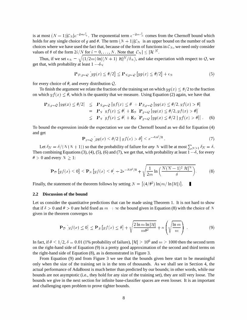
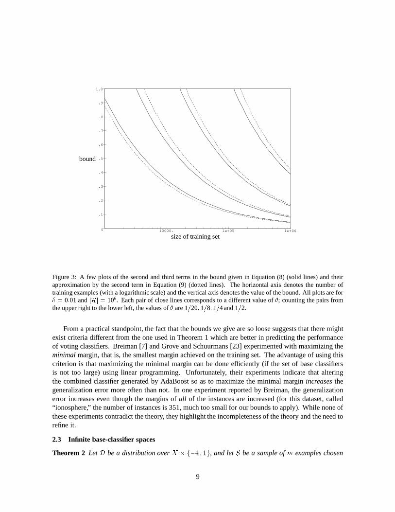
In fact, if � � 1=2, � = 0:01 (1% probability of failure), jHj � 106 and m � 1000 then the second termon the right-hand side of Equation (9) is a pretty good approximation of the second and third terms onthe right-hand side of Equation (8), as is demonstrated in Figure 3.
From Equation (9) and from Figure 3 we see that the bounds given here start to be meaningfulonly when the size of the training set is in the tens of thousands. As we shall see in Section 4, theactual performance of AdaBoost is much better than predicted by our bounds; in other words, while ourbounds are not asymptotic (i.e., they hold for any size of the training set), they are still very loose. Thebounds we give in the next section for infinite base-classifier spaces are even looser. It is an importantand challenging open problem to prove tighter bounds.
8
0
.1
.2
.3
.4
.5
.6
.7
.8
.9
1.0
bound
10000. 1e+05 1e+06
size of training set
Figure 3: A few plots of the second and third terms in the bound given in Equation (8) (solid lines) and theirapproximation by the second term in Equation (9) (dotted lines). The horizontal axis denotes the number oftraining examples (with a logarithmic scale) and the vertical axis denotes the value of the bound. All plots are for� = 0:01 and jHj = 106. Each pair of close lines corresponds to a different value of �; counting the pairs fromthe upper right to the lower left, the values of � are 1=20; 1=8; 1=4 and 1=2.
From a practical standpoint, the fact that the bounds we give are so loose suggests that there mightexist criteria different from the one used in Theorem 1 which are better in predicting the performanceof voting classifiers. Breiman [7] and Grove and Schuurmans [23] experimented with maximizing theminimal margin, that is, the smallest margin achieved on the training set. The advantage of using thiscriterion is that maximizing the minimal margin can be done efficiently (if the set of base classifiersis not too large) using linear programming. Unfortunately, their experiments indicate that alteringthe combined classifier generated by AdaBoost so as to maximize the minimal margin increases thegeneralization error more often than not. In one experiment reported by Breiman, the generalizationerror increases even though the margins of all of the instances are increased (for this dataset, called“ionosphere,” the number of instances is 351, much too small for our bounds to apply). While none ofthese experiments contradict the theory, they highlight the incompleteness of the theory and the need torefine it.
2.3 Infinite base-classifier spaces
Theorem 2 Let D be a distribution over X � f�1; 1g, and let S be a sample of m examples chosen
9
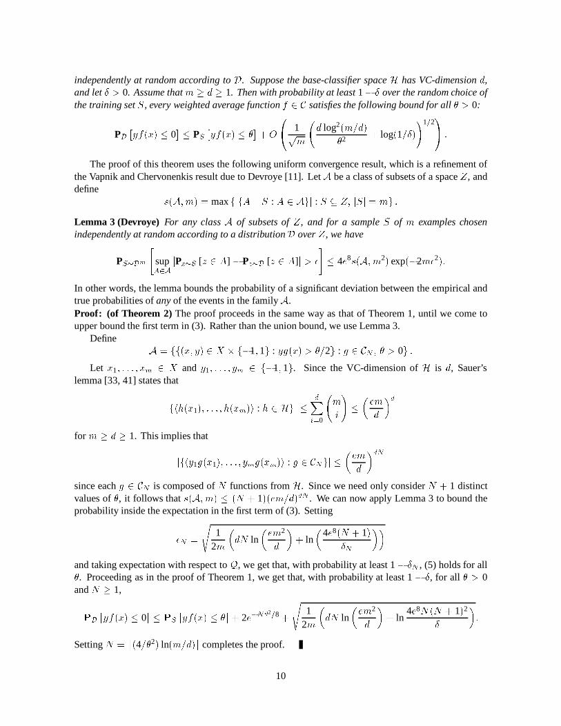
independently at random according to D. Suppose the base-classifier space H has VC-dimension d,and let � > 0. Assume that m � d � 1. Then with probability at least 1� � over the random choice ofthe training set S, every weighted average function f 2 C satisfies the following bound for all � > 0:
PD
�
yf(x) � 0�
� PS
�
yf(x) � �
�
+O
0
@
1p
m
d log2(m=d)
�
2 + log(1=�)
!1=21
A
:
The proof of this theorem uses the following uniform convergence result, which is a refinement ofthe Vapnik and Chervonenkis result due to Devroye [11]. Let A be a class of subsets of a space Z, anddefine
s(A; m) = max fjfA \ S : A 2 Agj : S � Z; jSj = mg :
Lemma 3 (Devroye) For any class A of subsets of Z, and for a sample S of m examples chosenindependently at random according to a distributionD over Z, we have
PS�D
m
"
supA2A
jPz�S
[z 2 A] � Pz�D
[z 2 A]j > �
#
� 4e8s(A; m
2) exp(�2m�
2):
In other words, the lemma bounds the probability of a significant deviation between the empirical andtrue probabilities of any of the events in the familyA.Proof: (of Theorem 2) The proof proceeds in the same way as that of Theorem 1, until we come toupper bound the first term in (3). Rather than the union bound, we use Lemma 3.
DefineA = ff(x; y) 2 X � f�1; 1g : yg(x) > �=2g : g 2 C
N
; � > 0g :
Let x1; : : : ; xm 2 X and y1; : : : ; ym 2 f�1; 1g. Since the VC-dimension of H is d, Sauer’slemma [33, 41] states that
jfhh(x1); : : : ; h(xm)i : h 2 Hgj �d
X
i=0
m
i
!
�
�
em
d
�
d
for m � d � 1. This implies that
jfhy1g(x1); : : : ; ymg(xm)i : g 2 CN
gj �
�
em
d
�
dN
since each g 2 C
N
is composed of N functions from H. Since we need only consider N + 1 distinctvalues of �, it follows that s(A; m) � (N + 1)(em=d)
dN . We can now apply Lemma 3 to bound theprobability inside the expectation in the first term of (3). Setting
�
N
=
s
12m
�
dN ln�
em
2
d
�
+ ln�
4e8(N + 1)�
N
��
and taking expectation with respect to Q, we get that, with probability at least 1� �
N
, (5) holds for all�. Proceeding as in the proof of Theorem 1, we get that, with probability at least 1 � �, for all � > 0and N � 1,
P
D
�
yf(x) � 0�
� P
S
�
yf(x) � �
�
+ 2e�N�
2=8
+
s
12m
�
dN ln�
em
2
d
�
+ ln4e8
N(N + 1)2
�
�
:
Setting N =
�
(4=�2) ln(m=d)
�
completes the proof.
10

2.4 Sketch of a more general approach
Instead of the proof above, we can use a more general approach which can also be applied to any classof real-valued functions. The use of an approximating class, such as C
N
in the proofs of Theorems 1and 2, is central to our approach. We refer to such an approximating class as a sloppy cover. Moreformally, for a class F of real-valued functions, a training set S of size m, and positive real numbers� and �, we say that a function class F̂ is an �-sloppy �-cover of F with respect to S if, for all f inF , there exists f̂ in F̂ with P
x�S
h
jf̂(x)� f(x)j > �
i
< �. Let N (F ; �; �;m) denote the maximum,over all training sets S of size m, of the size of the smallest �-sloppy �-cover of F with respect to S.Standard techniques yield the following theorem (the proof is essentially identical to that of Theorem 2in Bartlett [2]).
Theorem 4 Let F be a class of real-valued functions defined on the instance space X . Let D be adistribution over X � f�1; 1g, and let S be a sample of m examples chosen independently at randomaccording to D. Let � > 0 and let � > 0. Then the probability over the random choice of the trainingset S that there exists any function f 2 F for which
PD
�
yf(x) � 0�
> PS
�
yf(x) � �
�
+ �
is at most2N (F ; �=2; �=8; 2m) exp(��2
m=32):
Theorem 2 can now be proved by constructing a sloppy cover using the same probabilistic argumentas in the proof of Theorems 1 and 2, i.e., by choosing an element of C
N
randomly by sampling functionsfrom H. In addition, this result leads to a slight improvement (by log factors) of the main result ofBartlett [2], which gives bounds on generalization error for neural networks with real outputs in termsof the size of the network weights and the margin distribution.
3 The Effect of Boosting on Margin Distributions
We now give theoretical evidence that Freund and Schapire’s [20] AdaBoost algorithm is especiallysuited to the task of maximizing the number of training examples with large margin.
We briefly review their algorithm. We adopt the notation used in the previous section, and restrictour attention to the binary case.
Boosting works by sequentially rerunning a base learning algorithm, each time using a differentdistribution over training examples. That is, on each round t = 1; : : : ; T , a distributionD
t
is computedover the training examples, or, formally, over the set of indices f1; : : : ; mg. The goal of the base learningalgorithm then is to find a classifier h
t
with small error �t
= P
i�D
t
�
y
i
6= h
t
(x
i
)
�
. The distribution usedby AdaBoost is initially uniform (D1(i) = 1=m), and then is updated multiplicatively on each round:
D
t+1(i) =D
t
(i) exp(�yi
�
t
h
t
(x
i
))
Z
t
:
Here, �t
=
12 ln((1� �
t
)=�
t
) and Zt
is a normalization factor chosen so that Dt+1 sums to one. In our
case, Zt
can be computed exactly:
Z
t
=
m
X
i=1
D
t
(i) exp(�yi
�
t
h
t
(x
i
))
11
=
X
i:yi
=h
t
(x
i
)
D
t
(i)e
��
t
+
X
i:yi
6=h
t
(x
i
)
D
t
(i)e
�
t
= (1� �
t
)e
��
t
+ �
t
e
�
t
= 2q
�
t
(1� �
t
):
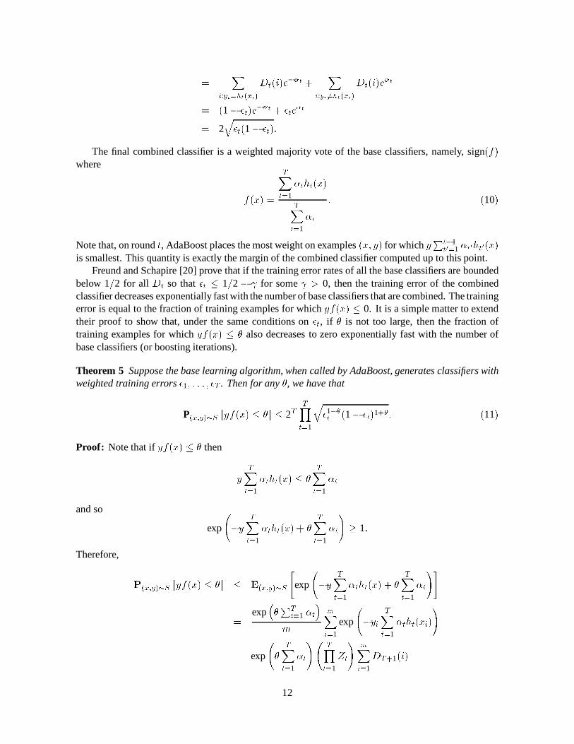
The final combined classifier is a weighted majority vote of the base classifiers, namely, sign(f)where
f(x) =
T
X
t=1
�
t
h
t
(x)
T
X
t=1
�
t
: (10)
Note that, on round t, AdaBoost places the most weight on examples (x; y) for which yP
t�1t
0
=1 �t0ht0(x)
is smallest. This quantity is exactly the margin of the combined classifier computed up to this point.Freund and Schapire [20] prove that if the training error rates of all the base classifiers are bounded
below 1=2 for all Dt
so that �t
� 1=2 � for some > 0, then the training error of the combinedclassifier decreases exponentially fast with the number of base classifiers that are combined. The trainingerror is equal to the fraction of training examples for which yf(x) � 0. It is a simple matter to extendtheir proof to show that, under the same conditions on �
t
, if � is not too large, then the fraction oftraining examples for which yf(x) � � also decreases to zero exponentially fast with the number ofbase classifiers (or boosting iterations).
Theorem 5 Suppose the base learning algorithm, when called by AdaBoost, generates classifiers withweighted training errors �1; : : : ; �T . Then for any �, we have that
P(x;y)�S
�
yf(x) � �
�
� 2TT
Y
t=1
q
�
1��t
(1� �
t
)
1+�: (11)
Proof: Note that if yf(x) � � then
y
T
X
t=1
�
t
h
t
(x) � �
T
X
t=1
�
t
and so
exp
�y
T
X
t=1
�
t
h
t
(x) + �
T
X
t=1
�
t
!
� 1:
Therefore,
P
(x;y)�S
�
yf(x) � �
�
� E
(x;y)�S
"
exp
�y
T
X
t=1
�
t
h
t
(x) + �
T
X
t=1
�
t
!#
=
exp�
�
P
T
t=1 �t
�
m
m
X
i=1
exp
�y
i
T
X
t=1
�
t
h
t
(x
i
)
!
= exp
�
T
X
t=1
�
t
!
T
Y
t=1
Z
t
!
m
X
i=1
D
T+1(i)
12

C4.5Boosting Bagging ECOC
letter
erro
r (%
)
10 100 100005
10152025303540
10 100 100005
10152025303540
10 100 100005
10152025303540
# classifiers
cum
ulat
ive
dist
ribu
tion
-1 -0.5 0.5 1
0.5
1.0
-1 -0.5 0.5 1
0.5
1.0
-1 -0.5 0.5 1
0.5
1.0
margin
satimage
erro
r (%
)
10 100 100005
10152025303540
10 100 100005
10152025303540
10 100 100005
10152025303540
# classifiers
cum
ulat
ive
dist
ribu
tion
-1 -0.5 0.5 1
0.5
1.0
-1 -0.5 0.5 1
0.5
1.0
-1 -0.5 0.5 1
0.5
1.0
margin
vehicle
erro
r (%
)
10 100 100005
10152025303540
10 100 100005
10152025303540
10 100 100005
10152025303540
# classifiers
cum
ulat
ive
dist
ribu
tion
-1 -0.5 0.5 1
0.5
1.0
-1 -0.5 0.5 1
0.5
1.0
-1 -0.5 0.5 1
0.5
1.0
margin
Figure 4: Error curves and margin distribution graphs for three voting methods (bagging, boosting and ECOC)using C4.5 as the base learning algorithm. Results are given for the letter, satimage and vehicle datasets. (Seecaption under Figure 1 for an explanation of these curves.)
13

decision stumpsBoosting Bagging ECOC
letter
erro
r (%
)
10 100 10000
20
40
60
80
100
10 100 10000
20
40
60
80
100
10 100 10000
20
40
60
80
100
# classifiers
cum
ulat
ive
dist
ribu
tion
-1 -0.5 0.5 1
0.5
1.0
-1 -0.5 0.5 1
0.5
1.0
-1 -0.5 0.5 1
0.5
1.0
margin
satimage
erro
r (%
)
10 100 10000
20
40
60
80
100
10 100 10000
20
40
60
80
100
10 100 10000
20
40
60
80
100
# classifiers
cum
ulat
ive
dist
ribu
tion
-1 -0.5 0.5 1
0.5
1.0
-1 -0.5 0.5 1
0.5
1.0
-1 -0.5 0.5 1
0.5
1.0
margin
vehicle
erro
r (%
)
10 100 10000
20
40
60
80
100
10 100 10000
20
40
60
80
100
10 100 10000
20
40
60
80
100
# classifiers
cum
ulat
ive
dist
ribu
tion
-1 -0.5 0.5 1
0.5
1.0
-1 -0.5 0.5 1
0.5
1.0
-1 -0.5 0.5 1
0.5
1.0
margin
Figure 5: Error curves and margin distribution graphs for three voting methods (bagging, boosting and ECOC)using decision stumps as the base learning algorithm. Results are given for the letter, satimage and vehicle datasets.(See caption under Figure 1 for an explanation of these curves.)
14

where the last equality follows from the definition of DT+1. Noting that
P
m
i=1 DT+1(i) = 1, andplugging in the values of �
t
and Zt
gives the theorem.
To understand the significance of the result, assume for a moment that, for all t, �t
� 1=2� forsome > 0. Since here we are considering only two-class prediction problems, a random predictionwill be correct exactly half of the time. Thus, the condition that �
t
� 1=2� for some small positive means that the predictions of the base classifiers are slightly better than random guessing. Given thisassumption, we can simplify the upper bound in Equation (11) to:
�
q
(1� 2 )1��(1 + 2 )1+�
�
T
:
If � < , it can be shown that the expression inside the parentheses is smaller than 1 so that theprobability that yf(x) � � decreases exponentially fast with T .4 In practice, �
t
increases as a functionof t, possibly even converging to 1=2. However, if this increase is sufficiently slow the bound ofTheorem 5 is still useful. Characterizing the conditions under which the increase is slow is an openproblem.
Although this theorem applies only to binary classification problems, Freund and Schapire [20] andothers [35, 36] give extensive treatment to the multiclass case (see also Section 4). All of their resultscan be extended to prove analogous theorems about margin distributions for this more general case.
4 More Margin Distribution Graphs
In this section, we describe experiments we conducted to produce a series of error curves and margindistribution graphs for a variety of datasets and learning methods.
Datasets. We used three benchmark datasets called “letter,” “satimage” and “vehicle.” Brief descrip-tions of these are given in Appendix B. Note that all three of these learning problems are multiclasswith 26, 6 and 4 classes, respectively.
Voting methods. In addition to bagging and boosting, we used a variant of Dietterich and Bakiri’s [13]method of error-correcting output codes (ECOC), which can be viewed as a voting method. Thisapproach was designed to handle multiclass problems using only a two-class learning algorithm. Briefly,it works as follows: As in bagging and boosting, a given base learning algorithm (which need onlybe designed for two-class problems) is rerun repeatedly. However, unlike bagging and boosting, theexamples are not reweighted or resampled. Instead, on each round, the labels assigned to each exampleare modified so as to create a new two-class labeling of the data which is induced by a simple mappingfrom the set of classes into f�1;+1g. The base learning algorithm is then trained using this relabeleddata, generating a base classifier.
The sequence of bit assignments for each of the individual labels can be viewed as a “code word.”A given test example is then classified by choosing the label whose associated code word is closest inHamming distance to the sequence of predictions generated by the base classifiers. This coding-theoreticinterpretation led Dietterich and Bakiri to the idea of choosing code words with strong error-correctingproperties so that they will be as far apart from one another as possible. However, in our experiments,rather than carefully constructing error-correcting codes, we simply used random output codes whichare highly likely to have similar properties.
4We can show that if is known in advance then an exponential decrease in the probability can be achieved (by a slightlydifferent boosting algorithm) for any � < 2 . However, we don’t know how to achieve this improvement when no nontriviallower bound on 1=2 � �
t
is known a priori.
15

The ECOC combination rule can also be viewed as a voting method: Each base classifier ht
, on agiven instance x, predicts a single bit h
t
(x) 2 f�1;+1g. We can interpret this bit as a single vote foreach of the labels which were mapped on round t to h
t
(x). The combined hypothesis then predicts withthe label receiving the most votes overall. Since ECOC is a voting method, we can measure marginsjust as we do for boosting and bagging.
As noted above, we used three multiclass learning problems in our experiments, whereas the versionof boosting given in Section 3 only handles two-class data. Freund and Schapire [20] describe astraightforward adaption of this algorithm to the multiclass case. The problem with this algorithm isthat it still requires that the accuracy of each base classifier exceed 1=2. For two-class problems, thisrequirement is about as minimal as can be hoped for since random guessing will achieve accuracy 1=2.However, for multiclass problems in which k > 2 labels are possible, accuracy 1=2 may be muchharder to achieve than the random-guessing accuracy rate of 1=k. For fairly powerful base learners,such as C4.5, this does not seem to be a problem. However, the accuracy 1=2 requirement can oftenbe difficult for less powerful base learning algorithms which may be unable to generate classifiers withsmall training errors.
Freund and Schapire [20] provide one solution to this problem by modifying the form of the baseclassifiers and refining the goal of the base learner. In this approach, rather than predicting a single classfor each example, the base classifier chooses a set of “plausible” labels for each example. For instance,in a character recognition task, the base classifier might predict that a particular example is either a “6,”“8” or “9,” rather than choosing just a single label. Such a base classifier is then evaluated using a“pseudoloss” measure which, for a given example, penalizes the base classifier (1) for failing to includethe correct label in the predicted plausible label set, and (2) for each incorrect label which is includedin the plausible set. The combined classifier, for a given example, then chooses the single label whichoccurs most frequently in the plausible label sets chosen by the base classifiers (possibly giving moreor less weight to some of the base classifiers). The exact form of the pseudoloss is under the control ofthe boosting algorithm, and the base learning algorithm must therefore be designed to handle changesin the form of the loss measure.
Base learning algorithms. In our experiments, for the base learning algorithm, we used C4.5. Wealso used a simple algorithm for finding the best single-node, binary-split decision tree (a decision“stump”). Since this latter algorithm is very weak, we used the “pseudoloss” versions of boosting andbagging, as described above. (See Freund and Schapire [20, 18] for details.)
Results. Figures 4 and 5 show error curves and margin distribution graphs for the three datasets, threevoting methods and two base learning algorithms. Note that each figure corresponds only to a singlerun of each algorithm.
As explained in the introduction, each of the learning curve figures shows the training error (bottom)and test error (top) curves. We have also indicated as horizontal grid lines the error rate of the baseclassifier when run just once, as well as the error rate of the combined classifier after 1000 iterations. Notethe log scale used in these figures. Margin distribution graphs are shown for 5, 100 and 1000 iterationsindicated by short-dashed, long-dashed (sometimes barely visible) and solid curves, respectively.
It is interesting that, across datasets, all of the learning algorithms tend to produce margin distributiongraphs of roughly the same character. As already noted, when used with C4.5, boosting is especiallyaggressive at increasing the margins of the examples, so much so that it is “willing” to suffer significantreductions in the margins of those examples that already have large margins. This can be seen inFigure 4, where we observe that the maximal margin in the final classifier is bounded well away from1. Contrast this with the margin distribution graphs after 1000 iterations of bagging in which as many
16
Kong & Dietterich [26] definitions Breiman [8] definitionsstumps C4.5 stumps C4.5
error pseudoloss error error pseudoloss errorname – boost bag boost bag – boost bag – boost bag boost bag – boost bagwaveform bias 26.0 3.8 22.8 0.8 11.9 1.5 0.5 1.4 19.2 2.6 15.7 0.5 7.9 0.9 0.3 1.4
var 5.6 2.8 4.1 3.8 8.6 14.9 3.7 5.2 12.5 4.0 11.2 4.1 12.5 15.5 3.9 5.2error 44.7 19.6 39.9 17.7 33.5 29.4 17.2 19.7 44.7 19.6 39.9 17.7 33.5 29.4 17.2 19.7
twonorm bias 2.5 0.6 2.0 0.5 0.2 0.5 1.3 0.3 1.1 0.3 0.1 0.3var 28.5 2.3 17.3 18.7 1.8 5.4 29.6 2.6 18.2 19.0 1.9 5.6error 33.3 5.3 21.7 21.6 4.4 8.3 33.3 5.3 21.7 21.6 4.4 8.3
threenorm bias 24.5 6.3 21.6 4.7 2.9 5.0 14.2 4.1 13.8 2.6 1.9 3.1var 6.9 5.1 4.8 16.7 5.2 6.8 17.2 7.3 12.6 18.8 6.3 8.6error 41.9 22.0 36.9 31.9 18.6 22.3 41.9 22.0 36.9 31.9 18.6 22.3
ringnorm bias 46.9 4.1 46.9 2.0 0.7 1.7 32.3 2.7 37.6 1.1 0.4 1.1var –7.9 6.6 –7.1 15.5 2.3 6.3 6.7 8.0 2.2 16.4 2.6 6.9error 40.6 12.2 41.4 19.0 4.5 9.5 40.6 12.2 41.4 19.0 4.5 9.5
Kong & bias 49.2 49.1 49.2 7.7 35.1 7.7 5.5 8.9 49.0 49.0 49.0 5.3 29.7 5.1 3.5 6.2Dietterich var 0.2 0.2 0.2 5.1 3.5 7.2 6.6 4.3 0.4 0.3 0.5 7.5 8.9 9.8 8.5 6.9
error 49.5 49.3 49.5 12.8 38.6 14.9 12.1 13.1 49.5 49.3 49.5 12.8 38.6 14.9 12.1 13.1
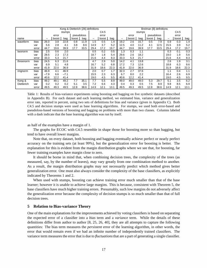
Table 1: Results of bias-variance experiments using boosting and bagging on five synthetic datasets (describedin Appendix B). For each dataset and each learning method, we estimated bias, variance and generalizationerror rate, reported in percent, using two sets of definitions for bias and variance (given in Appendix C). BothC4.5 and decision stumps were used as base learning algorithms. For stumps, we used both error-based andpseudoloss-based versions of boosting and bagging on problems with more than two classes. Columns labeledwith a dash indicate that the base learning algorithm was run by itself.
as half of the examples have a margin of 1.The graphs for ECOC with C4.5 resemble in shape those for boosting more so than bagging, but
tend to have overall lower margins.Note that, on every dataset, both boosting and bagging eventually achieve perfect or nearly perfect
accuracy on the training sets (at least 99%), but the generalization error for boosting is better. Theexplanation for this is evident from the margin distribution graphs where we see that, for boosting, farfewer training examples have margin close to zero.
It should be borne in mind that, when combining decision trees, the complexity of the trees (asmeasured, say, by the number of leaves), may vary greatly from one combination method to another.As a result, the margin distribution graphs may not necessarily predict which method gives bettergeneralization error. One must also always consider the complexity of the base classifiers, as explicitlyindicated by Theorems 1 and 2.
When used with stumps, boosting can achieve training error much smaller than that of the baselearner; however it is unable to achieve large margins. This is because, consistent with Theorem 5, thebase classifiers have much higher training errors. Presumably, such low margins do not adversely affectthe generalization error because the complexity of decision stumps is so much smaller than that of fulldecision trees.
5 Relation to Bias-variance Theory
One of the main explanations for the improvements achieved by voting classifiers is based on separatingthe expected error of a classifier into a bias term and a variance term. While the details of thesedefinitions differ from author to author [8, 25, 26, 40], they are all attempts to capture the followingquantities: The bias term measures the persistent error of the learning algorithm, in other words, theerror that would remain even if we had an infinite number of independently trained classifiers. Thevariance term measures the error that is due to fluctuations that are a part of generating a single classifier.
17

The idea is that by averaging over many classifiers one can reduce the variance term and in that wayreduce the expected error.
In this section, we discuss a few of the strengths and weaknesses of bias-variance theory as anexplanation for the performance of voting methods, especially boosting.
5.1 The bias-variance decomposition for classification.
The origins of bias-variance analysis are in quadratic regression. Averaging several independentlytrained regression functions will never increase the expected error. This encouraging fact is nicelyreflected in the bias-variance separation of the expected quadratic error. Both bias and variance arealways nonnegative and averaging decreases the variance term without changing the bias term.
One would naturally hope that this beautiful analysis would carry over from quadratic regression toclassification. Unfortunately, as has been observed before us, (see, for instance, Friedman [22]) takingthe majority vote over several classification rules can sometimes result in an increase in the expectedclassification error. This simple observation suggests that it may be inherently more difficult or evenimpossible to find a bias-variance decomposition for classification as natural and satisfying as in thequadratic regression case.
This difficulty is reflected in the myriad definitions that have been proposed for bias and variance [8,25, 26, 40]. Rather than discussing each one separately, for the remainder of this section, except wherenoted, we follow the definitions given by Kong and Dietterich [26], and referred to as “Definition 0” byBreiman [8]. (These definitions are given in Appendix C.)
5.2 Bagging and variance reduction.
The notion of variance certainly seems to be helpful in understanding bagging; empirically, baggingappears to be most effective for learning algorithms with large variance. In fact, under idealizedconditions, variance is by definition the amount of decrease in error effected by bagging a large numberof base classifiers. This ideal situation is one in which the bootstrap samples used in bagging faithfullyapproximate truly independent samples. However, this assumption can fail to hold in practice, in whichcase, bagging may not perform as well as expected, even when variance dominates the error of the baselearning algorithm.
This can happen even when the data distribution is very simple. As a somewhat contrived example,consider data generated according to the following distribution. The label y 2 f�1;+1g is chosenuniformly at random. The instance x 2 f�1;+1g7 is then chosen by picking each of the 7 bits to beequal to y with probability 0:9 and�y with probability 0:1. Thus, each coordinate ofx is an independentnoisy version of y. For our base learner, we use a learning algorithm which generates a classifier that isequal to the single coordinate of x which is the best predictor of y with respect to the training set. It isclear that each coordinate of x has the same probability of being chosen as the classifier on a randomtraining set, so the aggregate predictor over many independently trained samples is the unweightedmajority vote over the coordinates of x, which is also the Bayes optimal predictor in this case. Thus, thebias of our learning algorithm is exactly zero. The prediction error of the majority rule is roughly 0:3%,and so a variance of about 9:7% strongly dominates the expected error rate of 10%. In such a favorablecase, one would predict, according to the bias-variance explanation, that bagging could get close to theerror of the Bayes optimal predictor.
However, using a training set of 500 examples, the generalization error achieved by bagging is 5:6%after 200 iterations. (All results are averaged over many runs.) The reason for this poor performanceis that, in any particular random sample, some of the coordinates of x are slightly more correlated with
18
y and bagging tends to pick these coordinates much more often than the others. Thus, in this case, thebehavior of bagging is very different from its expected behavior on truly independent training sets.
Boosting, on the same data, achieved a test error of 0:6%.
5.3 Boosting and variance reduction.
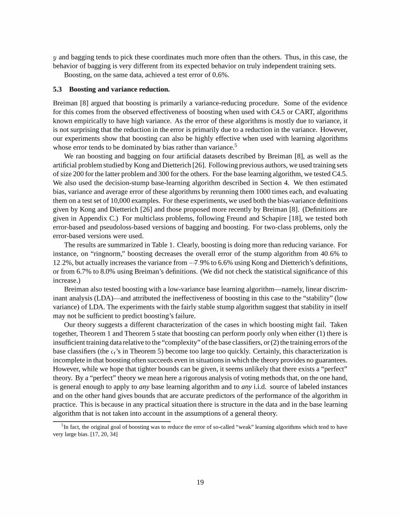
Breiman [8] argued that boosting is primarily a variance-reducing procedure. Some of the evidencefor this comes from the observed effectiveness of boosting when used with C4.5 or CART, algorithmsknown empirically to have high variance. As the error of these algorithms is mostly due to variance, itis not surprising that the reduction in the error is primarily due to a reduction in the variance. However,our experiments show that boosting can also be highly effective when used with learning algorithmswhose error tends to be dominated by bias rather than variance.5
We ran boosting and bagging on four artificial datasets described by Breiman [8], as well as theartificial problem studied by Kong and Dietterich [26]. Following previous authors, we used training setsof size 200 for the latter problem and 300 for the others. For the base learning algorithm, we tested C4.5.We also used the decision-stump base-learning algorithm described in Section 4. We then estimatedbias, variance and average error of these algorithms by rerunning them 1000 times each, and evaluatingthem on a test set of 10,000 examples. For these experiments, we used both the bias-variance definitionsgiven by Kong and Dietterich [26] and those proposed more recently by Breiman [8]. (Definitions aregiven in Appendix C.) For multiclass problems, following Freund and Schapire [18], we tested botherror-based and pseudoloss-based versions of bagging and boosting. For two-class problems, only theerror-based versions were used.
The results are summarized in Table 1. Clearly, boosting is doing more than reducing variance. Forinstance, on “ringnorm,” boosting decreases the overall error of the stump algorithm from 40:6% to12:2%, but actually increases the variance from�7:9% to 6.6% using Kong and Dietterich’s definitions,or from 6.7% to 8.0% using Breiman’s definitions. (We did not check the statistical significance of thisincrease.)
Breiman also tested boosting with a low-variance base learning algorithm—namely, linear discrim-inant analysis (LDA)—and attributed the ineffectiveness of boosting in this case to the “stability” (lowvariance) of LDA. The experiments with the fairly stable stump algorithm suggest that stability in itselfmay not be sufficient to predict boosting’s failure.
Our theory suggests a different characterization of the cases in which boosting might fail. Takentogether, Theorem 1 and Theorem 5 state that boosting can perform poorly only when either (1) there isinsufficient training data relative to the “complexity” of the base classifiers, or (2) the training errors of thebase classifiers (the �
t
’s in Theorem 5) become too large too quickly. Certainly, this characterization isincomplete in that boosting often succeeds even in situations in which the theory provides no guarantees.However, while we hope that tighter bounds can be given, it seems unlikely that there exists a “perfect”theory. By a “perfect” theory we mean here a rigorous analysis of voting methods that, on the one hand,is general enough to apply to any base learning algorithm and to any i.i.d. source of labeled instancesand on the other hand gives bounds that are accurate predictors of the performance of the algorithm inpractice. This is because in any practical situation there is structure in the data and in the base learningalgorithm that is not taken into account in the assumptions of a general theory.
5In fact, the original goal of boosting was to reduce the error of so-called “weak” learning algorithms which tend to havevery large bias. [17, 20, 34]
19

5.4 Why averaging can increase complexity
In this section, we challenge a common intuition which says that when one takes the majority voteover several base classifiers the generalization error of the resulting classifier is likely to be lower thanthe average generalization error of the base classifiers. In this view, voting is seen as a method for“smoothing” or “averaging” the classification rule. This intuition is sometimes based on the bias-variance analysis of regression described in the previous section. Also, to some, it seems to follow froma Bayesian point of view according to which integrating the classifications over the posterior is betterthan using any single classifier. If one feels comfortable with these intuitions, there seems to be littlepoint to most of the analysis given in this paper. It seems that because AdaBoost generates a majorityvote over several classifiers, its generalization error is, in general, likely to be better than the averagegeneralization error of the base classifiers. According to this point of view, the suggestion we make inthe introduction that the majority vote over many classifiers is more complex than any single classifierseems to be irrelevant and misled.
In this section, we describe a base learning algorithm which, when combined using AdaBoost, islikely to generate a majority vote over base classifiers whose training error goes to zero, while at thesame time the generalization error does not improve at all. In other words, it is a case in which votingresults in over-fitting. This is a case in which the intuition described above seems to break down, whilethe margin-based analysis developed in this paper gives the correct answer.
Suppose we use classifiers that are delta-functions, i.e., they predict +1 on a single point in the inputspace and �1 everywhere else, or vice versa (�1 on one point and +1 elsewhere). (If you dislike delta-functions, you can replace them with nicer functions. For example, if the input space isRn, use balls ofsufficiently small radius and make the prediction +1 or�1 inside, and�1 or +1, respectively, outside.)To this class of functions we add the constant functions that are �1 everywhere or +1 everywhere.
Now, for any training sample of size m we can easily construct a set of at most 2m functions fromour class such that the majority vote over these functions will always be correct. To do this, we associateone delta function with each training example; the delta function gives the correct value on the trainingexample and the opposite value everywhere else. Letting m
+
and m
�
denote the number of positiveand negative examples, we next add m
+
copies of the function which predicts +1 everywhere, and m�
copies of the function which predicts�1 everywhere. It can now be verified that the sum (majority vote)of all these functions will be positive on all of the positive examples in the training set, and negative onall the negative examples. In other words, we have constructed a combined classifier which exactly fitsthe training set.
Fitting the training set seems like a good thing; however, the very fact that we can easily fit such arule to any training set implies that we don’t expect the rule to be very good on independently drawnpoints outside of the training set. In other words, the complexity of these average rules is too large,relative to the size of the sample, to make them useful. Note that this complexity is the result ofaveraging. Each one of the delta rules is very simple (the VC-dimension of this class of functions isexactly 2), and indeed, if we found a single delta function (or constant function) that fit a large samplewe could, with high confidence, expect the rule to be correct on new randomly drawn examples.
How would boosting perform in this case? It can be shown using Theorem 5 (with � = 0) thatboosting would slowly but surely find a combination of the type described above having zero trainingerror but very bad generalization error. A margin-based analysis of this example shows that while allof the classifications are correct, they are correct only with a tiny margin of size O(1=m), and so wecannot expect the generalization error to be very good.
20

h
h(x)High dimensional spaceInput space R
θ−
+
− − −
−−
+++
++
−
−
−
−−
−
+++
+++
+
+−
α
Figure 6: The maximal margins classification method. In this example, the raw data point x is an element of R,but in that space the positive and negative examples are not linearly separable. The raw input is mapped to a pointin a high dimensional space (here R2) by a fixed nonlinear transformation ~
h. In the high dimensional space, theclasses are linearly separable. The vector ~� is chosen to maximize the minimal margin �. The circled instancesare the support vectors; Vapnik shows that ~� can always be written as a linear combination of the support vectors.
6 Relation to Vapnik’s Maximal Margin Classifiers
The use of the margins of real-valued classifiers to predict generalization error was previously studiedby Vapnik [42] in his work with Boser and Guyon [5] and Cortes [10] on optimal margin classifiers.
We start with a brief overview of optimal margin classifiers. One of the main ideas behind thismethod is that some nonlinear classifiers on a low dimensional space can be treated as linear classifiersover a high dimensional space. For example, consider the classifier that labels an instance x 2 R as+1 if 2x5
� 5x2+ x > 10 and �1 otherwise. This classifier can be seen as a linear classifier if we
represent each instance by the vector ~h(x) :
= (1; x; x2; x
3; x
4; x
5). If we set ~� = (�10; 1;�5; 0; 0; 2)
then the classification is +1 when ~� �
~
h(x) > 0 and �1 otherwise. In a typical case, the data consistsof about 10; 000 instances in R100 which are mapped into R1;000;000. Vapnik introduced the methodof kernels which provides an efficient way for calculating the predictions of linear classifiers in thehigh dimensional space. Using kernels, it is usually easy to find a linear classifier that separates thedata perfectly. In fact, it is likely that there are many perfect linear classifiers, many of which mighthave very poor generalization ability. In order to overcome this problem, the prescription suggested byVapnik is to find the classifier that maximizes the minimal margin. More precisely, suppose that thetraining sample S consists of pairs of the form (x; y) where x is the instance and y 2 f�1;+1g is itslabel. Assume that ~h(x) is some fixed nonlinear mapping of instances into Rn (where n is typicallyvery large). Then the maximal margin classifier is defined by the vector ~� which maximizes
min(x;y)2S
y(~� �
~
h(x))
jj~�jj2: (12)
Here, jj~�jj2 is the l2 or Euclidean norm of the vector ~�. A graphical sketch of the maximal marginmethod is given in Figure 6. For the analysis of this method, Vapnik assumes that all of the vectors ~h(x)are enclosed within a ball of radius R, i.e., they all are within Euclidean distance R from some fixedvector in Rn. Without loss of generality, we can assume that R = 1.
21

Vapnik [42] showed that the VC dimension of all linear classifiers with minimum margin at least � isupper bounded by 1=�2. This result implies bounds on the generalization error in terms of the expectedminimal margin on test points which do not depend on the dimension n of the space into which thedata are mapped. However, typically, the expected value of the minimal margin is not known. Shawe-Taylor et al. [38] used techniques from the theory of learning real-valued functions to give bounds ongeneralization error in terms of margins on the training examples. Shawe-Taylor et al. [39] also gaverelated results for arbitrary real classes.
Consider the relation between Equation (10) and the argument of the minimum in Equation (12). Wecan view the coefficients f�
t
g
T
t=1 as the coordinates of a vector ~� 2 RT and the predictions fht
(x)g
T
t=1
as the coordinates of the vector ~h(x) 2 f�1;+1gT . Then we can rewrite Equation (10) as
f(x) =
~� �
~
h(x)
k~�k1;
where jj~�jj1 =
P
T
t=1 j�tj is the l1 norm of ~�. In our analysis, we use the fact that all of the componentsof ~h(x) are in the range [�1;+1], or, in other words that the max or l
1
norm of ~h(x) is bounded by 1:k
~
h(x)k
1
= maxTt=1 jht(x)j � 1.
Viewed this way, the connection between maximal margin classifiers and boosting becomes clear.Both methods aim to find a linear combination in a high dimensional space which has a large margin onthe instances in the sample. The norms used to define the margin are different in the two cases and theprecise goal is also different—maximal margin classifiers aim to maximize the minimal margin whileboosting aims to minimize an exponential weighting of the examples as a function of their margins.Our interpretation for these differences is that boosting is more suited for the case when the mapping~
h maps x into a high dimensional space where all of the coordinates have a similar maximal range,such as f�1;+1g. On the other hand, the optimal margin method is suitable for cases in which theEuclidean norm of~h(x) is likely to be small, such as is the case when~h is an orthonormal transformationbetween inner-product spaces. Related to this, the optimal margin method uses quadratic programmingfor its optimization, whereas the boosting algorithm can be seen as a method for approximate linearprogramming [7, 19, 21, 23].
Both boosting and support vector machines aim to find a linear classifier in a very high dimensionalspace. However, computationally, they are very different: support vector machines use the method ofkernels to perform computations in the high dimensional space while boosting relies on a base learningalgorithm which explores the high dimensional space one coordinate at a time.
Vapnik [42] gave an alternative analysis of optimal margin classifiers, based on the number ofsupport vectors, i.e., the number of examples that define the final classifier. This analysis is preferableto the analysis that depends on the size of the margin when only a few of the training examples aresupport vectors. Previous work [17] has suggested that boosting also can be used as a method forselecting a small number of “informative” examples from the training set. Investigating the relevanceof this type of bound when applying boosting to real-world problems is an interesting open researchdirection.
7 Other loss functions
We describe briefly related work which has been done on loss functions other than the 0-1 loss.For quadratic loss, Jones [24] and Barron [1] have shown that functions in the convex hull of a class
H of real-valued functions can be approximated by a convex combination of N elements of H to anaccuracy of O(1=N) by iteratively adding the member of H which minimizes the residual error to theexisting convex combination. Lee, Bartlett and Williamson [27] extended this result to show that the
22
procedure will converge to the best approximation in the convex hull ofH even when the target functionis not in the convex hull ofH. Lee, Bartlett and Williamson [27, 28] also studied the generalization errorwhen this procedure is used for learning. In results analogous to those presented here, they showed thatthe generalization error can be bounded in terms of the sum of the absolute values of the output weights(when the members of H are normalized to have output values in the interval [�1; 1]), rather than interms of the number of components in the convex combination.
Similar work on iterative convex approximation in Lp
spaces was presented by Donahue et al. [14].To the best of our knowledge, similar iterative schemes for combining functions have not been studiedfor the log loss.
Extensions of boosting to solve regression problems have been suggested by Freund [17] and Freundand Schapire [20]. These extensions are yet to be tested in practice. Drucker [15] experimented with adifferent extension of boosting for regression and reported some encouraging results.
8 Open Problems
The methods in this paper allow us to upper bound the generalization error of a voted classifier basedon simple statistics which can be measured using the training data. These statistics are a function of theempirical distribution of the margins. While our bounds seem to explain the experiments qualitatively,their quantitative predictions are greatly over pessimistic. The challenge of coming up with betterbounds can be divided into two questions. First, can one give better bounds that are a function of theempirical margins distribution? Second, are there better bounds that are functions of other statistics?
A different approach to understanding the behavior of AdaBoost is to find functions of the trainingset which predict the generalization error well on all or most of the datasets encountered in practice.While this approach does not give one the satisfaction of a mathematical proof, it might yield goodresults in practice.
Acknowledgments
Many thanks to Leo Breiman for a poignant email exchange which challenged us to think harder aboutthese problems. Thanks also to all those who contributed to the datasets used in this paper, and to thethree anonymous reviewers for many helpful criticisms.
References
[1] Andrew R. Barron. Universal approximation bounds for superposition of a sigmoidal function.IEEE Transactions on Information Theory, 39(3):930–945, 1993.
[2] Peter L. Bartlett. The sample complexity of pattern classification with neural networks: the sizeof the weights is more important than the size of the network. IEEE Transactions on InformationTheory, 1998 (to appear).
[3] Eric Bauer and Ron Kohavi. An empirical comparison of voting classification algorithms: Bagging,boosting, and variants. Unpublished manuscript, 1997.
[4] Eric B. Baum and David Haussler. What size net gives valid generalization? Neural Computation,1(1):151–160, 1989.
[5] Bernhard E. Boser, Isabelle M. Guyon, and Vladimir N. Vapnik. A training algorithm for optimalmargin classifiers. In Proceedings of the Fifth Annual ACM Workshop on Computational LearningTheory, pages 144–152, 1992.
[6] Leo Breiman. Bagging predictors. Machine Learning, 24(2):123–140, 1996.[7] Leo Breiman. Prediction games and arcing classifiers. Technical Report 504, Statistics Department,
University of California at Berkeley, 1997.
23

[8] Leo Breiman. Arcing classifiers. Annals of Statistics, to appear.[9] Leo Breiman, Jerome H. Friedman, Richard A. Olshen, and Charles J. Stone. Classification and
Regression Trees. Wadsworth International Group, 1984.[10] Corinna Cortes and Vladimir Vapnik. Support-vector networks. Machine Learning, 20(3):273–
297, September 1995.[11] Luc Devroye. Bounds for the uniform deviation of empirical measures. Journal of Multivariate
Analysis, 12:72–79, 1982.[12] Thomas G. Dietterich. An experimental comparison of three methods for constructing ensembles
of decision trees: Bagging, boosting, and randomization. Unpublished manuscript, 1998.[13] Thomas G. Dietterich and Ghulum Bakiri. Solving multiclass learning problems via error-
correcting output codes. Journal of Artificial Intelligence Research, 2:263–286, January 1995.[14] M. J. Donahue, L. Gurvits, C. Darken, and E. Sontag. Rates of convex approximation in non-Hilbert
spaces. Constructive Approximation, 13:187–220, 1997.[15] Harris Drucker. Improving regressors using boosting techniques. In Machine Learning: Proceed-
ings of the Fourteenth International Conference, pages 107–115, 1997.[16] Harris Drucker and Corinna Cortes. Boosting decision trees. In Advances in Neural Information
Processing Systems 8, pages 479–485, 1996.[17] Yoav Freund. Boosting a weak learning algorithm by majority. Information and Computation,
121(2):256–285, 1995.[18] Yoav Freund and Robert E. Schapire. Experiments with a new boosting algorithm. In Machine
Learning: Proceedings of the Thirteenth International Conference, pages 148–156, 1996.[19] Yoav Freund and Robert E. Schapire. Game theory, on-line prediction and boosting. In Proceedings
of the Ninth Annual Conference on Computational Learning Theory, pages 325–332, 1996.[20] Yoav Freund and Robert E. Schapire. A decision-theoretic generalization of on-line learning and
an application to boosting. Journal of Computer and System Sciences, 55(1):119–139, August1997.
[21] Yoav Freund and Robert E. Schapire. Adaptive game playing using multiplicative weights. Gamesand Economic Behavior, (to appear).
[22] Jerome H. Friedman. On bias, variance, 0/1-loss, and the curse-of-dimensionality. Availableelectronically from http://stat.stanford.edu/�jhf.
[23] Adam J. Grove and Dale Schuurmans. Boosting in the limit: Maximizing the margin of learnedensembles. In Proceedings of the Fifteenth National Conference on Artificial Intelligence, 1998.
[24] Lee K. Jones. A simple lemma on greedy approximation in Hilbert space and convergence ratesfor projection pursuit regression and neural network training. Annals of Statistics, 20(1):608–613,1992.
[25] Ron Kohavi and David H. Wolpert. Bias plus variance decomposition for zero-one loss functions.In Machine Learning: Proceedings of the Thirteenth International Conference, pages 275–283,1996.
[26] Eun Bae Kong and Thomas G. Dietterich. Error-correcting output coding corrects bias andvariance. In Proceedings of the Twelfth International Conference on Machine Learning, pages313–321, 1995.
[27] Wee Sun Lee, Peter L. Bartlett, and Robert C. Williamson. Efficient agnostic learning of neuralnetworks with bounded fan-in. IEEE Transactions on Information Theory, 42(6):2118–2132,1996.
[28] Wee Sun Lee, Peter L. Bartlett, and Robert C. Williamson. The importance of convexity in learningwith squared loss. IEEE Transactions on Information Theory, to appear.
24

[29] Richard Maclin and David Opitz. An empirical evaluation of bagging and boosting. In Proceedingsof the Fourteenth National Conference on Artificial Intelligence, pages 546–551, 1997.
[30] C. J. Merz and P. M. Murphy. UCI repository of machine learning databases, 1998.http://www.ics.uci.edu/�mlearn/MLRepository.html.
[31] J. R. Quinlan. Bagging, boosting, and C4.5. In Proceedings of the Thirteenth National Conferenceon Artificial Intelligence, pages 725–730, 1996.
[32] J. Ross Quinlan. C4.5: Programs for Machine Learning. Morgan Kaufmann, 1993.[33] N. Sauer. On the density of families of sets. Journal of Combinatorial Theory Series A, 13:145–147,
1972.[34] Robert E. Schapire. The strength of weak learnability. Machine Learning, 5(2):197–227, 1990.[35] Robert E. Schapire. Using output codes to boost multiclass learning problems. In Machine
Learning: Proceedings of the Fourteenth International Conference, pages 313–321, 1997.[36] Robert E. Schapire and Yoram Singer. Improved boosting algorithms using confidence-rated
predictions. In Proceedings of the Eleventh Annual Conference on Computational LearningTheory, 1998.
[37] Holger Schwenk and Yoshua Bengio. Training methods for adaptive boosting of neural networksfor character recognition. In Advances in Neural Information Processing Systems 10, 1998.
[38] John Shawe-Taylor, Peter L. Bartlett, Robert C. Williamson, and Martin Anthony. A frameworkfor structural risk minimisation. In Proceedings of the Ninth Annual Conference on ComputationalLearning Theory, pages 68–76, 1996.
[39] John Shawe-Taylor, Peter L. Bartlett, Robert C. Williamson, and Martin Anthony. Structural riskminimization over data-dependent hierarchies. Technical Report NC-TR-96-053, Neurocolt, 1996.
[40] Robert Tibshirani. Bias, variance and prediction error for classification rules. Technical report,University of Toronto, November 1996.
[41] V. N. Vapnik and A. Ya. Chervonenkis. On the uniform convergence of relative frequencies ofevents to their probabilities. Theory of Probability and its applications, XVI(2):264–280, 1971.
[42] Vladimir N. Vapnik. The Nature of Statistical Learning Theory. Springer, 1995.
A Generalization Error for Multiclass Problems
In this appendix, we describe how Theorems 1 and 2 can be extended to multiclass problems.Suppose there are k classes, and define Y = f1; 2; : : : ; kg as the output space. We formally view
the base classifiers h 2 H as mappings from X�Y to f0; 1g, with the interpretation that if h(x; y) = 1then y is predicted by h to be a plausible label for x. This general form of classifier covers the forms ofbase classifiers used throughout this paper. For simple classifiers, like the decision trees computed byC4.5, only a single label is predicted so that, for each x, h(x; y) = 1 for exactly one label y. However,some of the other combination methods — such as pseudoloss-based boosting or bagging, as well asDietterich and Bakiri’s output-coding method — use base classifiers which vote for a set of plausiblelabels so that h(x; y) may be 1 for several labels y.
We define the convex hull C of H as
C
:
=
8
<
:
f : (x; y) 7!X
h2H
a
h
h(x; y)
�
�
�
�
�
a
h
� 0;X
h
a
h
= 1
9
=
;
;
so a classifier f in C predicts label y for input x if f(x; y) > maxy
0
6=y
f(x; y
0
) (and ties are brokenarbitrarily). We define the margin of an example (x; y) for such a function f as
margin(f; x; y) = f(x; y)�maxy
0
6=y
f(x; y
0
): (13)
25

Clearly, f gives the wrong prediction on (x; y) only if margin(f; x; y) � 0. With these definitions, wehave the following generalization of Theorems 1 and 2.
Theorem 6 Let D be a distribution over X � Y , and let S be a sample of m examples chosenindependently at random according to D. Assume that the base-classifier space H is finite, and let� > 0. Then with probability at least 1� � over the random choice of the training set S, every functionf 2 C satisfies the following bound for all � > 0:
PD
�
margin(f; x; y) � 0�
� PS
�
margin(f; x; y) � �
�
+O
1p
m
�
log(mk) log jHj�
2 + log(1=�)�1=2
!
:
More generally, for finite or infiniteHwith VC-dimensiond, the following bound holds as well, assumingthat m � d � 1:
PD
�
margin(f; x; y) � 0�
� PS
�
margin(f; x; y) � �
�
+O
0
@
1p
m
d log2(mk=d)
�
2 + log(1=�)
!1=21
A
:
Proof: The proof closely follows that of Theorem 1, so we only describe the differences. We firstconsider the case of finite H.
First, we define
C
N
:
=
(
f : (x; y) 7!1N
N
X
i=1
h
i
(x; y)
�
�
�
�
�
h
i
2 H
)
:
As in the proof of Theorem 1, for any f 2 C we choose an approximating function g 2 CN
accordingto the distributionQ, and we have
P
D
�
margin(f; x; y)� 0�
� E
g�Q
�
P
D
�
margin(g; x; y)� �=2��
+E
D
�
P
g�Q
�
margin(g; x; y)> �=2 j margin(f; x; y) � 0��
:
We bound the second term of the right hand side as follows: Fix f , x and y, and let y0 6= y achieve themaximum in Equation (13) so that
margin(f; x; y) = f(x; y)� f(x; y
0
):
Clearly, margin(g; x; y)� g(x; y)� g(x; y
0
) and
E
g�Q
�
g(x; y)� g(x; y
0
)
�
= f(x; y)� f(x; y
0
)
so
P
g�Q
�
margin(g; x; y)> �=2 j margin(f; x; y) � 0�
� P
g�Q
�
g(x; y)� g(x; y
0
) > �=2 j f(x; y)� f(x; y
0
) � 0�
� e
�N�
2=8
using the Chernoff bound.
26

Equations (5) and (6) follow exactly as in the proof of Theorem 1 with yf(x) and yg(x) replacedby margin(f; x; y) and margin(g; x; y). We can derive the analog of Equation (7) as follows:
P
g�Q
�
margin(g; x; y)� �=2 j margin(f; x; y) > �
�
= P
g�Q
�
9y
0
6= y : g(x; y)� g(x; y
0
) � �=2 j 8y0 6= y : f(x; y)� f(x; y
0
) > �
�
�
X
y
0
6=y
P
g�Q
�
g(x; y)� g(x; y
0
) � �=2 j f(x; y)� f(x; y
0
) > �
�
� (k� 1)e�N�
2=8:
Proceeding as in the proof of Theorem 1, we see that, with probability at least 1� �, for any � > 0and N � 1,
P
D
�
margin(f; x; y) � 0�
� P
S
�
margin(f; x; y) � �
�
+ ke
�N�
2=8
+
s
12m
ln�
N(N + 1)2jHj
N
�
�
:
Setting N =
�
(4=�2) ln(mk
2= ln jHj)
�
gives the result.For infinite H, we follow essentially the same modifications to the argument above as used in the
proof of Theorem 2. As before, to apply Lemma 3, we need to derive an upper bound on s(A; m) where
A = ff(x; y) 2 X � Y : margin(g; x; y)> �=2g : g 2 CN
; � > 0g :
Let x1; : : : ; xm 2 X and y1; : : : ; ym 2 Y . Then applying Sauer’s lemma to the set f(xi
; y) : 1 � i �
m; y 2 Y g gives
jfhh(x1; 1); : : : ; h(x1; k); : : : ; h(xm; 1); : : : ; h(xm
; k)i : h 2 Hgj �d
X
i=0
km
i
!
�
�
emk
d
�
d
:
This implies that
jfhg(x1; 1); : : : ; g(x1; k); : : : ; g(xm; 1); : : : ; g(xm
; k)i : g 2 CN
gj �
�
emk
d
�
dN
;
and hence
jf(margin(g; x1; y1); : : : ;margin(g; xm
; y
m
)) : g 2 CN
gj �
�
emk
d
�
dN
:
Thus, s(A; m) � (N + 1)(emk=d)
dN . Proceeding as before, we obtain the bound
P
D
�
margin(f; x; y) � 0�
� P
S
�
margin(f; x; y) � �
�
+ ke
�N�
2=8
+
s
12m
�
dN ln�
em
2k
d
�
+ ln4e8
N(N + 1)2
�
�
:
Setting N as above completes the proof.
B Brief Descriptions of Datasets
In this appendix, we briefly describe the datasets used in our experiments.
27

# examples # #name train test classes featuresvehicle 423 423 4 18satimage 4435 2000 6 36letter 16000 4000 26 16
Table 2: The three benchmark machine-learning problems used in the experiments.
B.1 Non-synthetic datasets
In Section 4, we conducted experiments on three non-synthetic datasets called “letter,” “satimage” and“vehicle.” All three are available from the repository at the University of California at Irvine [30].
Some of the basic characteristics of these datasets are given in Table 2. The letter and satimagedatasets came with their own test sets. For the vehicle dataset, we randomly selected half of the data tobe held out as a test set. All features are continuous (real-valued). None of these datasets have missingvalues.
The letter benchmark is a letter image recognition task. The dataset was created by David J. Slate.According to the documentation provided with this dataset, “The objective is to identify each of a largenumber of black-and-white rectangular pixel displays as one of the 26 capital letters in the Englishalphabet. The character images were based on 20 different fonts and each letter within these 20 fontswas randomly distorted to produce a file of 20,000 unique stimuli. Each stimulus was converted into 16primitive numerical attributes (statistical moments and edge counts) which were then scaled to fit intoa range of integer values from 0 through 15.”
The satimage dataset is the statlog version of a satellite image dataset. According to the docu-mentation, “This database consists of the multi-spectral values of pixels in 3 � 3 neighborhoods in asatellite image, and the classification associated with the central pixel in each neighborhood. The aimis to predict this classification, given the multi-spectral values... The original database was generatedfrom Landsat Multi-Spectral Scanner image data... purchased from NASA by the Australian Center forRemote Sensing, and used for research at The Center for Remote Sensing... The sample database wasgenerated taking a small section (82 rows and 100 columns) from the original data. The binary valueswere converted to their present ASCII form by Ashwin Srinivasan. The classification for each pixelwas performed on the basis of an actual site visit by Ms. Karen Hall, when working for Professor JohnA. Richards.... Conversion to 3� 3 neighborhoods and splitting into test and training sets was done byAlistair Sutherland....”
The purpose of the vehicle dataset, according to its documentation, is “to classify a given silhouetteas one of four types of vehicle, using a set of features extracted from the silhouette. The vehicle maybe viewed from one of many different angles... This dataset comes from the Turing Institute... The[extracted] features were a combination of scale independent features utilizing both classical momentsbased measures such as scaled variance, skewness and kurtosis about the major/minor axes and heuristicmeasures such as hollows, circularity, rectangularity and compactness. Four ‘Corgie’ model vehicleswere used for the experiment: a double decker bus, Chevrolet van, Saab 9000 and an Opel Manta 400....The images were acquired by a camera looking downwards at the model vehicle from a fixed angle ofelevation....”
28
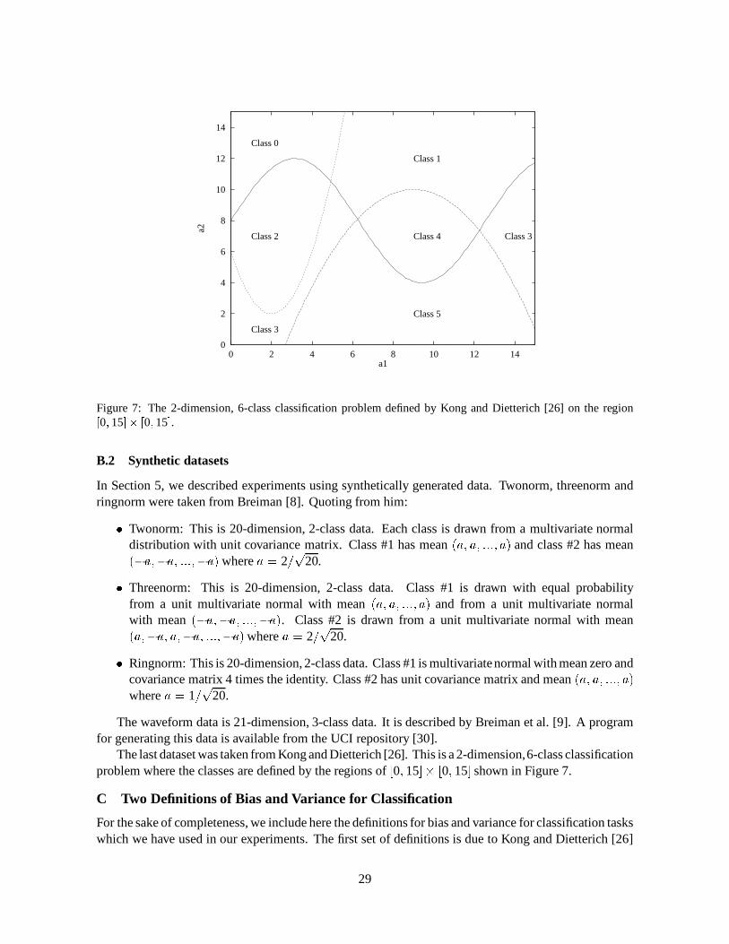
0
2
4
6
8
10
12
14
0 2 4 6 8 10 12 14
a2
a1
Class 0
Class 1
Class 2
Class 3
Class 3Class 4
Class 5
Figure 7: The 2-dimension, 6-class classification problem defined by Kong and Dietterich [26] on the region[0; 15]� [0; 15].
B.2 Synthetic datasets
In Section 5, we described experiments using synthetically generated data. Twonorm, threenorm andringnorm were taken from Breiman [8]. Quoting from him:
� Twonorm: This is 20-dimension, 2-class data. Each class is drawn from a multivariate normaldistribution with unit covariance matrix. Class #1 has mean (a; a; :::; a) and class #2 has mean(�a;�a; :::;�a) where a = 2=
p
20.
� Threenorm: This is 20-dimension, 2-class data. Class #1 is drawn with equal probabilityfrom a unit multivariate normal with mean (a; a; :::; a) and from a unit multivariate normalwith mean (�a;�a; :::;�a). Class #2 is drawn from a unit multivariate normal with mean(a;�a; a;�a; :::;�a)where a = 2=
p
20.
� Ringnorm: This is 20-dimension, 2-class data. Class #1 is multivariatenormal with mean zero andcovariance matrix 4 times the identity. Class #2 has unit covariance matrix and mean (a; a; :::; a)
where a = 1=p
20.
The waveform data is 21-dimension, 3-class data. It is described by Breiman et al. [9]. A programfor generating this data is available from the UCI repository [30].
The last dataset was taken from Kong and Dietterich [26]. This is a 2-dimension,6-class classificationproblem where the classes are defined by the regions of [0; 15]� [0; 15] shown in Figure 7.
C Two Definitions of Bias and Variance for Classification
For the sake of completeness, we include here the definitions for bias and variance for classification taskswhich we have used in our experiments. The first set of definitions is due to Kong and Dietterich [26]
29

and the second one is due to Breiman [8]. Assume that we have an infinite supply of independenttraining sets S of sizem. Each sampleS is drawn i.i.d. from a fixed distributionD over X�f1; : : : ; kgwhere k is the number of classes. Denote by C
S
the classifier that is generated by the base learningalgorithm given the sample S. Denote by C
A
the classification rule that results from running the baselearning algorithm on an infinite number of independent training sets and taking the plurality vote6 overthe resulting classifiers. Finally denote by C
� the Bayes optimal prediction rule for the distributionD. The prediction of a classifier C on an instance x 2 X is denoted C(x) and the expected error of aclassifier C is denoted
PE(C)
:
= P
(x;y)�D
�
C(x) 6= y
�
:
The definitions of Kong and Dietterich are:
Bias :
= PE(C
A
)� PE(C
�
) ;
Variance :
= E
S�D
m
�
PE(C
S
)
�
� PE(C
A
) :
Breiman defines a partition of the sample space into two sets. The “unbiased” set U consists of allx 2 X for which C
A
(x) = C
�
(x) and the “biased” set B is U ’s complement. Given these sets thedefinition of bias and variance are:
Bias :
= P
(x;y)�D
�
C
�
(x) = y; x 2 B
�
�E
S�D
m
h
P
(x;y)�D
�
C
S
(x) = y; x 2 B
�
i
;
Variance :
= P
(x;y)�D
�
C
�
(x) = y; x 2 U
�
� E
S�D
m
h
P
(x;y)�D
�
C
S
(x) = y; x 2 U
�
i
:
6The plurality vote outputs the class which receives the largest number of votes, breaking ties uniformly at random. Whenk = 2 the plurality vote is equal to the majority vote.
30


![Opinion Mining in a Telephone Survey Corpus Presenter: Shih-Hsiang Reference: [1]Robert E. Schapire and Yoram Singer. BoosTexter : A boosting-based system.](https://static.fdocuments.us/doc/165x107/551708aa55034603568b5238/opinion-mining-in-a-telephone-survey-corpus-presenter-shih-hsiang-reference-1robert-e-schapire-and-yoram-singer-boostexter-a-boosting-based-system.jpg)