Boosting Support Vector Machines

Elkin García, Fernando Lozano

Departamento de Ingeniería Eléctrica y ElectrónicaUniversidad de los Andes, Bogotá, Colombia.

{ elkin-ga, flozano } @ uniandes.edu.co

Abstract. This paper presents a classification algorithm based on Sup-port Vector Machines classifiers combined with Boosting techniques. Thisclassifier presents a better performance in training time, a similar gener-alization and a similar model complexity but the model representationis more compact.

1 Introduction

Support Vector Machines (SVM) have been applied successfully in many prob-lems in classification and regression [1]. It has been shown recently that for someof the kernel functions used in practice [2] SVMs are strong learners, in the sensethat they can achieve a generalization error arbitrarily close to the Bayes errorwith a sufficiently large training set.

The main disadvantage of using SVMs is that the running time of trainingalgorithms do not scale well with the size of the training set . If m is the size of thetraining set, training an SVM involves solving a quadratic program (QP) of sizem2, which takes O(m3) with a general purposed QP solver. Multiple researchershave proposed some methods that improve this running time to O(m2) [3,4,5,6].

On the other hand, boosting algorithms like Adaboost [7] find a good hypoth-esis combining appropriately hypothesis produced by a weak (or base) learner.Roughly, a weak learner is a learner that returns a hypothesis that outperformrandom guessing.

Using a classifier that is already strong (like SVM) as the base learner inAdaboost does not seem to offer significant advantages in terms of generalizationerror. In fact, Wickramaratna, Holden and Buxton have used SVM as the baseclassifier of Adaboost and have reported that the performance of the classifierdecreases as the number of rounds increases [8]. However, as we will show below,a weakened version of SVM can still be useful as a base classifier. As shownin [9] the size of the weights assigned by Adaboost to the weak SVMs, serve asan indication of which data points are likely to become support vectors in thefinal model, and hence can be useful in the implementation of editing algorithms.

This paper is organized as follows. Section 2 reviews basic concepts of clas-sification as well as the basics of Boosting algorithms and the SVM algorithm.In Section 3 we present the new algorithm Boosting Support Vector Machines(BSVM). Section 4 presents experiments using the new algorithm on real worlddata. Finally, section 5 presents the conclusions of this work.

2 Preliminaries

Let X be an input space, Y a space of labels and ∆ a distribution over XxY.Let S={〈xi, yi〉}m

i=1 be a set of labeled examples where each pair xi, yi is drawni.i.d. according to ∆. For a binary classification problem the space of labels isrestricted to Y = {−1,+1}.

A classification rule, also called hypothesis, is a function h : X 7→ Y. Thehypothesis assigns a label to elements of the input space. In the binary classi-fication problem the hypothesis is h : X 7→ [−1,+1], where the sign of h(x) isinterpreted as the predicted label of x and the magnitude |h(x)| is interpretedas the “confidence” in this prediction. Let H denote a class of hypothesis.

The performance of the hypothesis is evaluated using the generalization errorR and the empirical error Remp:

R(h) = P(x,y∼∆){sgn(h(x)) 6= y} (1)

Remp(h,S,D) =m∑

i=1

D(i)Jsign(h(xi)) 6= yiK (2)

Where D ∈ Rm is a discrete distribution over the set S and J·K is the indicatorfunction.

A learning algorithm is an efficient algorithm that takes as inputs a set Sof labeled examples and a discrete distribution D ∈ Rm over S and returnsa hypothesis h ∈ H. A combined classifier H(x) is a convex combination ofseverals hypothesis hi. This is

H(x) =T∑

i=1

αihi(x) (3)

Where αi ≥ 0 and∑T

i=1 αi = 1. Each hypothesis hi is a base classifier.

2.1 Boosting

Boosting algorithms improve the performance of a learning algorithm by com-bining several hypothesis in a proper manner. In particular, the Adaboost algo-rithm constructs a linear combination of hypothesis that are produced by callinga weak learner in a succession of rounds. At each iteration t, Adaboost makesa call to the weak learner Weak with input set S and distribution Dt and re-turns a hypothesis ht. The distribution Dt is updated so that the weights of theexamples that ht misclassifies are reduced and the weight of the examples thatht classifies correctly are increased. In this way, in the next iteration the weaklearner is forced to focus its attention in the examples that have been misclas-sified more often in previous rounds. Figure 1 shows this algorithm as it waspresented in [10].

Algorithm: Adaboost (S, D1, T,Weak)Input: S = {xi, yi}mi=1, D1, T , Weak(·, ·)Output: H(·)for t = 1 to T do

Obtain a weak hypothesis using Dt.ht ←Weak(S, Dt).Select αt ∈ R. Usually:

αt =1

2ln

(1−Remp(ht,S, Dt)

Remp(ht,S, Dt)

). (4)

Update:

Dt+1(i) =Dt(i)exp(−αtyiht(xi))

Zt. (5)

where Zt is a normalization factor so that Dt+1 will be a distribution.end

Return final hypothesis:

H(x) = sign

(T∑

t=1

αt∑t αt

ht(x)

). (6)

Fig. 1: Algoritmo Adaboost.

2.2 Support Vector Machines

The aim of Support Vector Machines in the binary classification problem is tofind the optimal separating hyperplane (this is the hyperplane that maximizesthe geometric margin) in a high dimensional feature space X ′. This space isrelated to the input space X by a nonlinear transformation Φ(x). The idea ofthis transformation is to project the data to a space where it is approximatelyseparable by a linear threshold function.

When the data is not linearly separable the problem of finding the linearthreshold function with the smallest classification error is NP-Hard [11]. Theidea in SVMs is to allow some of the examples to be misclassified while keepinga large margin in the remaining data.

Cortes and Vapnik [12, 13] suggest to solve the following optimization prob-lem. This formulation is known as C−SVM :

minw∈X ′,ξ∈Rm

b∈R

τ(w, ξ, ρ) =12‖w‖2

X ′ +C

m

m∑i=1

ξi

s.t. yi(〈w, Φ(xi)〉X ′ + b) ≥ 1− ξi

ξi ≥ 0 for i = 1, . . . ,m

(7)

where C > 0 is a constant that controls the “trade-off” between minimizingthe training error and maximizing the margin. A positive slack variable ξi > 0indicates a classification mistake. It is more convenient to look at this problemin its dual form:

minα∈Rm

f(α) =12αT Qα− eT α

s.t. yT α = 0

0 ≤ αi ≤C

mfor i = 1, . . . ,m

(8)

where Qij=yiyjk(xi, xj), k(xi, xj)=〈Φ(xi), Φ(xj)〉X ′ is a positive defined ker-nel and e is a vector of ones. The solution of this problem has the form:

hw,b(x) = sgn

(m∑

i=1

yiαik(x, xi) + b

)(9)

Note that in the solution in feature space X ′ the training examples appearonly through the kernel function. Data points for which αi 6= 0, are called supportvectors.

Schölkopf et. al. [14] propose a modification to the optimization problem (8).Here, the parameter C is replaced by the parameter ν ∈ (0, 1]. This new problemis known as ν-SVM

minw∈X ′,ξ∈Rm

ρ,b∈R

τ(w, ξ, ρ) =12‖w‖2

X ′ − νρ +1m

m∑i=1

ξi

s.t. yi(〈w, Φ(xi)〉X ′ + b) ≥ ρ− ξi

ξi ≥ 0 for i = 1, . . . ,mρ ≥ 0

(10)

In this optimization problem, a new parameter ρ controls the margin betweenthe classes. If ξ = 0 then the first restriction of (10) establishes a margin of2ρ/ ‖w‖. An advantage of this formulation is that ν is an upper bound of thetraining error and a lower bound of the number of support vectors if ρ > 0. Thedual problem of (10) is

minα∈Rm

f(α) =12αT Qα

s.t. yT α = 0

0 ≤ αi ≤1m

for i = 1, . . . ,m

eT α ≥ ν

(11)

Where Qij and e are the same as (8) and the final hypothesis is defined in(9).

Even for moderate values of m the quadratic programs (8) and (11) are noteasily solvable with generic QP solvers. Several methods have been proposedinstead.Chunking techniques proposed initially by Vapnik [3], are based in twoobservations: 1) Removing training examples with αi = 0 do not change thesolution of the QP problem. 2) A decomposition of the original problem (8)in smaller problems is easier and more efficient. Some of the algorithms basedon these observations are [4, 5]. Platt [6] proposes a technique called SecuentialMinimal Optimization (SMO) where the original problem is chunked in QPproblems of two variables, that have analytical solution.

Problem (11) includes an additional inequality constraint. Crisp and Burges[15] and Chang and Lin [16] have shown that eT α ≥ ν can be replaced byeT α = ν without changing the solution, and the techniques described beforecan be adapted.

Joachims [5] employs a combination of SMO with shrinking and cachingtechniques to solve (8) and (11), that results in a running time that is betweenquadratic and cubic ,depending on the peculiarities of the problem. The com-putational complexity is basically dominated by the number of kernel evalua-tions [17].

3 Boosting Support Vector Machines

The running time of training algorithms for SVMs can be reduced if only afew training examples are involved in the actual computations. This fact can beexploited by Adaboost if at each iteration most of the weight in the distributionpassed to the weak learner is assigned to a few data points.

The computation time can be reduced as follows. If the complexity of theoriginal training algorithm is bounded by Amx with A ∈ R then training with afraction νm is bounded by A(νm)x. Thus, training q hypothesis is bounded byAq(νm)x (assuming the overhead introduced by Adaboost is negligible). Thenif x > 1, 0 > ν > 1 and q ≤ 1/ν

Aq(νm)x ≤ A

ν(νm)x = Aνx−1mx ≤ Amx (12)

The complexity of this algorithm is still O(mx) but the constant is smaller.For this reason is useful to make a Boosting algorithm similar to Adaboost

using SVM as a weak learner. Then, it is necessary to modify the optimizationproblems (8) and (11) in therms of distributions and to guarantee that SVM isa weak learner.

3.1 Support Vector Machines for distributions

Let D be a discrete distribution over the set of labeled examples S={〈xi, yi〉}mi=1.

We want to incorporate this information in the optimization problem solved byC-SVM and ν-SVM.

A simple way of doing this is to use bootstrap samples of the original set drawnaccording to D [18]. A serious drawback of this method is that the matrix Q in(8) and (11) may become ill conditioned because examples with large weight inthe distribution may appear several times in a bootstrap sample.

A better option is to modify the original optimization problem to incorporatedirectly the distribution. We present two alternatives of solution. The first al-ternative is to penalize the slack variables ξi proportional to Di in the objectivefunction. The optimization problem in C-SVM becomes:

minw∈X ′,ξ∈Rm

b∈R

τ(w, ξ, ρ) =12‖w‖2

X ′ +C

m

m∑i=1

Diξi

s.t. yi(〈w, Φ(xi)〉X ′ + b) ≥ 1− ξi

ξi ≥ 0 for i = 1, . . . ,m

(13)

And the optimization problem in ν-SVM is:

minw∈X ′,ξ∈Rm

ρ,b∈R

τ(w, ξ, ρ) =12‖w‖2

X ′ − νρ +1m

m∑i=1

Diξi

s.t. yi(〈w, Φ(xi)〉X ′ + b) ≥ ρ− ξi

ξi ≥ 0 for i = 1, . . . ,m

ρ ≥ 0

(14)

The dual problems of (13) and (14) are respectively

minα∈Rm

f(α) =12αT Qα− eT α

s.t. yT α = 00 ≤ αi ≤ CDi for i = 1, . . . ,m

(15)

minα∈Rm

f(α) =12αT Qα

s.t. yT α = 00 ≤ αi ≤ Di for i = 1, . . . ,m

eT α ≥ ν

(16)

The second alternative is to include the distribution in the objetive functionbut also force examples with larger weights to have large margin. The modifiedC-SVM and ν-SVM formulations are:

minw∈X ′,ξ∈Rm

b∈R

τ(w, ξ, ρ) =12‖w‖2

X ′ +C

m

m∑i=1

Diξi

s.t. yi(〈w, Φ(xi)〉X ′ + b) ≥ mDi(1− ξi)ξi ≥ 0 for i = 1, . . . ,m

(17)

minw∈X ′,ξ∈Rm

ρ,b∈R

τ(w, ξ, ρ) =12‖w‖2

X ′ − νρ +1m

m∑i=1

Diξi

s.t. yi(〈w, Φ(xi)〉X ′ + b) ≥ mDi(ρ− ξi)ξi ≥ 0 for i = 1, . . . ,m

ρ ≥ 0

(18)

The dual problems of (17) and (18) are respectively:

minα∈Rm

f(α) =12αT Qα−mDT α

s.t. yT α = 0

0 ≤ αi ≤C

mfor i = 1, . . . ,m

(19)

minα∈Rm

f(α) =12αT Qα

s.t. yT α = 0

0 ≤ αi ≤1m

for i = 1, . . . ,m

mDT α ≥ ν

(20)

Where Qij=yiyjk(xi, xj) and D is the distribution vector.

3.2 Support Vector Machines like a Weak Learner

As mentioned before, a strong learner like SVM does not work well as the baselearner of Adaboost. However, a version of SVM that has been weakened can beuseful.

The idea is to discard a percentage µ of the examples in the original data set,and solve the optimization problem with a smaller training set. This will workas long as the training error on the whole data set remains under 50%. Thus,the idea is to discard the less representative examples in the data set, namelythe examples with small weight under the current distribution. Then, the subsetJ ⊆ S is defined by

∑j∈J Dj ≤ (1 − µ) where J has minimum cardinality.

Algorithm: WSVM(S,D,SV M ,kernel, C or ν, µ)Input: S = {xi, yi}mi=1, D, SV M(·, ·), kernel, C or ν, µOutput: h(·)Select J so that

∑j∈J Dj ≤ (1− µ) and J has minimum cardinality

Select S∗ = {〈xj , yj〉}J and D∗ = Dj

Obtain a weak hypothesis using D∗

h← SV M(S∗, D∗, kernel, C o ν) =

m∑i=1

yiβik(x, xi) + b

Fig. 2: Weakened SVM Algorithm.

Notice that as D becomes more askew in later rounds of Adaboost, more andmore data points are discarded, reducing dramatically the training time of thebase SVM learners. The new algorithm is presented in 2.

If we use an universal kernel (a kernel is universal if every set of points infeature space is separable using this kernel) we can obtains a bound on thepercentage of rejected data µ. This universal kernel is a strong learner withrespect to subset J . Then, we can obtain a classifier that has an error of at mostε (for small epsilon) and that in the worst case errs on all the elements of J ′ .Provided that SVM is a weak learner we have that (1− µ)ε + µ < 1/2 where

µ <1/2− ε

1− ε(21)

Thus, µ is close to 50%. However the bound is not tight because the elementsof J and J ′ are correlated and hence the classification rule obtained with Jdoes not have a large error on the set J ′ as long as the number of elements inJ is large enough. For this reason, µ is left as a parameter of the algorithm.Notice that an appropriate value for this parameter can be determined usingsome model selection strategy.

3.3 Boosting Support Vector Machines

The weakened SVM can be incorporated directly into Adaboost, obtaining acombined classifier of the form:

HT (x) = sgn

(T∑

i=1

αt∑t αt

sgn

(m∑

i=1

yiαik(x, xi) + b

))(22)

Notice however that 22 is not a hyperplane in feature space and that thecomplexity of the hypothesis HT (x) is larger than the complexity of the SVMin (9).

Algorithm: BSVM (S, D1, T, WSV M, µ, kernel, C or ν)

Input: S = {xi, yi}mi=1, D1, T , WSV M ,µ,kernel,C or νOutput: H(·)

H(x)←WSV M(S, D1, kernel, C or ν) =

m∑i=1

yiβ1,ik(x, xi) + b1

for t = 2 to T or stopping condition do

Dt =Dt−1(i)

(1−Remp(ht−1,S,Dt−1)

Remp(ht−1,S,Dt−1)

)− 12 ytht

Zt−1

Where Zt−1 is a nomalization factor so that Dt will be a distribution.

ht(x)←WSV M(S, Dt, kernel, C or ν) =

m∑i=1

yiβt,ik(x, xi) + bt

H(x, α) = αht(x) + (1− α)H(x)

Choose αt ∈ [0, 1] so that αt = arg min (Remp (H(α, x),S, D1))

H(x) = H(x, αt)

end

Return final hypothesis: H(x) = sgn (H(x))

Fig. 3: Algorithm BSVM.

For this reason, we modify the Adaboost algorithm shown in figure 1 so thatthe combined classifier has the form 9. This new algorithm that we will refer toas BSVM is detailed on figure 3.

Algorithm BSVM keeps the same general structure of Adaboost. The maindifference is that the final hypothesis is expressed as a hyperplane in featurespace. The computation of the coefficients αt of each hypothesis is also different:At each iteration, we compute the value of αt that minimizes the training errorover the convex combination of the current hypothesis ht(x) and the combinedhypothesis of the previous iteration H(x). This optimization problem can beeasily solved by numeric methods such as golden search or cubic interpolation.

The stopping condition of BSVM can be set so that the algorithms haltswhen it can no longer improve, i.e. when the error of the combined classifier cannot be decreased further. This can be accomplished by stopping when αt ≈ 0 orwhen Remp(H(x),S, D1) = 0.

From the generalization point of view it may be better to stop the algorithmwhen it starts over fitting the data. This can be done by checking the behavior ofthe empirical error on an independent cross validation set. Another alternative isto look at the slope of the training error and stop the algorithm when it becomes(approximately) flat. We can compute:

Remp.train[t− 1]−Remp.train[t]Remp.train[t− 1]

≤ f [t] (23)

where f [t] is non increasing.

4 Experiments

In this section, we present some experiments demonstrating the performance ofour algorithm on synthetic and real world data sets.

The data sets we utilize are the following:

– The MNIST data set of handwritten digits [19]. To restrict the problem tobinary classification, we consider the separation between digits 3 and 8. Thisis a relatively difficult task, with high dimensionality and moderately largenumber of examples.

– The synthetic data set Four-norm is a binary classification problem in 20dimensions. In this problem, examples from one class are drawn from oneof two normal distributions with equal probability. The normal distributionshave identity covariance matrix and means (a, a, ..., a) and (−a,−a, ...,−a).Similarly, examples from the second class are drawn from one of two normaldistributions with equal probability, identity covariance matrix and means(a,−a, ..., a,−a) and (−a, a, ...,−a, a). In this case we set a =

√2.

– Data sets Breast cancer, diabetes and australian from the UCI repository.[20].

For data sets that do not have test examples we set apart 10% of the datafor testing. In all experiments we utilize gaussian kernels k(xi, xj) = exp(−‖xi−xj‖2/σ). A summary of the data sets and the settings of the parameters of thegaussian kernel is shown in table 1.

Table 1: Data sets description

Database # Training # Testing Dimension σ

Elements Elements

MNIST 11982 1984 784 4M

Four norm 1000 10000 20 1k

Breast Cancer 615 68 9 100k

Diabetes 692 76 8 40

Australian 621 69 14 10

To train the SVM with distributions (i.e. solve problems (15) and (16)),we follow a strategy similar to the used by the SMO algorithm [6] and theimprovements suggested by others authors [17,16].

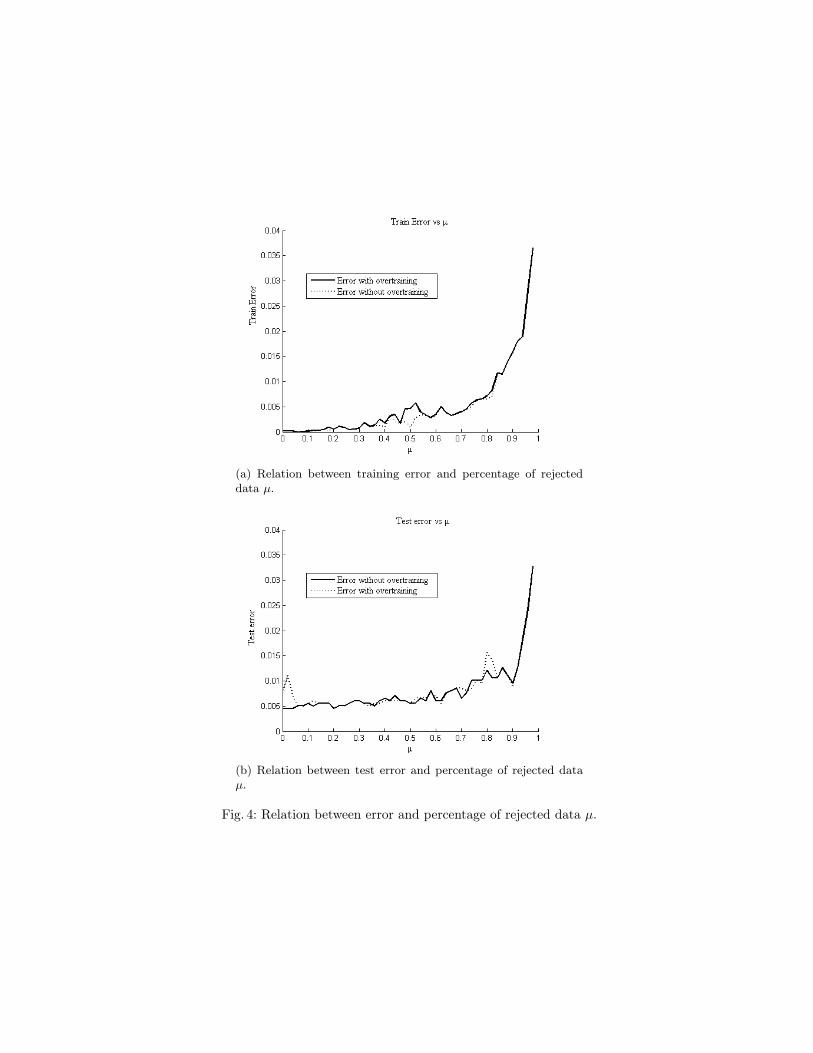
(a) Relation between training error and percentage of rejecteddata µ.

(b) Relation between test error and percentage of rejected dataµ.

Fig. 4: Relation between error and percentage of rejected data µ.

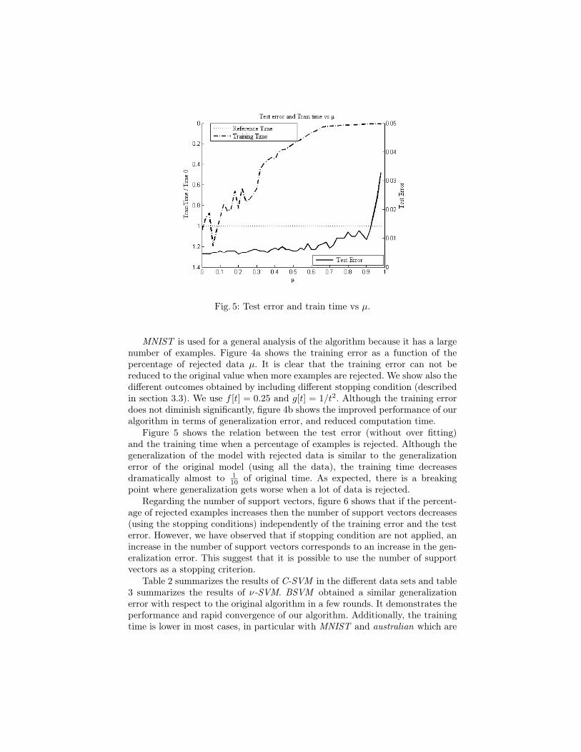
Fig. 5: Test error and train time vs µ.

MNIST is used for a general analysis of the algorithm because it has a largenumber of examples. Figure 4a shows the training error as a function of thepercentage of rejected data µ. It is clear that the training error can not bereduced to the original value when more examples are rejected. We show also thedifferent outcomes obtained by including different stopping condition (describedin section 3.3). We use f [t] = 0.25 and g[t] = 1/t2. Although the training errordoes not diminish significantly, figure 4b shows the improved performance of ouralgorithm in terms of generalization error, and reduced computation time.

Figure 5 shows the relation between the test error (without over fitting)and the training time when a percentage of examples is rejected. Although thegeneralization of the model with rejected data is similar to the generalizationerror of the original model (using all the data), the training time decreasesdramatically almost to 1

10 of original time. As expected, there is a breakingpoint where generalization gets worse when a lot of data is rejected.

Regarding the number of support vectors, figure 6 shows that if the percent-age of rejected examples increases then the number of support vectors decreases(using the stopping conditions) independently of the training error and the testerror. However, we have observed that if stopping condition are not applied, anincrease in the number of support vectors corresponds to an increase in the gen-eralization error. This suggest that it is possible to use the number of supportvectors as a stopping criterion.

Table 2 summarizes the results of C-SVM in the different data sets and table3 summarizes the results of ν-SVM. BSVM obtained a similar generalizationerror with respect to the original algorithm in a few rounds. It demonstrates theperformance and rapid convergence of our algorithm. Additionally, the trainingtime is lower in most cases, in particular with MNIST and australian which are

Fig. 6: Number of Support Vectors vs µ.

Table 2: Results of C-SVM

Database C Test Error µ # Test Error TimeBSVM

SVM (%) Iterations BSVM (%) /TimeSVM

MNIST 10 0.45 0.64 3 0.60 0.0762

Four norm 50 23.50 0.60 4 20.77 0.5212

200 19.68 0.60 4 18.48 0.5617

B. Cancer 100 0.00 0.7 3 0.00 0.9286

Diabetes 50 19.74 0.7 3 22.37 0.3636

Australian 100 18.84 0.7 3 15.94 0.135

Table 3: Results of ν-SVM

Database ν Test Error µ # Test Error TimeBSVM

SVM (%) Iterations BSVM (%) /TimeSVM

MNIST 0.15 4.83 0.60 3 4.54 0.6554

Four norm 0.3 21.05 0.60 4 26.06 0.8532

B. Cancer 0.4 1.47 0.80 3 0.00 1.52

Diabetes 0.2 26.32 0.80 3 26.32 1.13

Australian 0.4 15.94 0.80 3 13.04 0.76

large sets of high dimensionality. Finally, in general, algorithm C-BSVM is moreefficient than ν-BSVM.

Table 4: Number Support Vectors Comparison

Database C # S. Vectors # S. Vectors ν # S. Vectors # S. VectorsCSVM CBSVM ν SVM ν BSVM

MNIST 10 1417 1012 0.15 1817 1175

Four norm 200 688 454 0.3 340 395

Breast Cancer 100 78 46 0.4 216 58

Diabetes 50 327 147 0.2 121 50

Australian 100 202 104 0.4 245 93

The relation between the number of support vectors is shown in table 4.BSVM obtains a reduced number of support vectors while maintaining the samegeneralization error. There is a large reduction in no separable classes with largeBayes error, four-norm and diabetes are examples of this reduction.

5 Conclusions

The proposed algorithm BSVM combined efficiently SVM classifiers using Boost-ing techniques. This new algorithm does not increase the complexity of the finalhypothesis while decreasing the training time specially when the training set islarge or the dimensionality of the data is high.

The models produced by our algorithms are more compact because they haveless support vectors.

The proposed strategies for over fitting are effective because BSVM presentssimilar values of generalization with respect to the original implementation.

Problems for future research are finding tighter theoretical bounds on thepercentage of rejected examples and finding more exact stopping conditions.

References

1. Schölkopf, B., Smola, A.: Learning With Kernels. MIT Press, Cambridge, MA(2002)

2. Steinwart, I.: Sparness of support vector machines –some asymptotically sharpbounds. In Thrun, S., Saul, L., Schölkopf, B., eds.: Advances in Neural InformationProcessing Systems. Volume 16., Cambridge, MA, MIT Press (2004) 169–184

3. Vapnik, V.: Estimation of Dependences Based on Empirical Data [in Russian].Nauka, Moscow (1979) (English translation: Springer Verlag, New York, 1982).

4. Osuna, E., Freund, R., Girosi, F.: An improved training algorithm for supportvector machines. In Principe, J., Gile, L., Morgan, N., Wilson, E., eds.: NeuralNetworks for Signal Processing VII — Proceedings of the 1997 IEEE Workshop,New York, IEEE (1997) 276 – 285

5. Joachims, T.: Making large–scale SVM learning practical. In Schölkopf, B., Burges,C.J.C., Smola, A.J., eds.: Advances in Kernel Methods — Support Vector Learning,Cambridge, MA, MIT Press (1999) 169–184

6. Platt, J.: Fast training of support vector machines using sequential minimal opti-mization. In Schölkopf, B., Burges, C.J.C., Smola, A.J., eds.: Advances in KernelMethods — Support Vector Learning, Cambridge, MA, MIT Press (1999) 185–208

7. Freund, Y., Schapire, R.E.: A decision-theoretic generalization of on-line learningand an application to boosting. Journal of Computer and System Sciences 55(1997) 119–139

8. Wickramaratna, J., Holden, S., Buxton, B.: Performance degradation in boosting.In Kittler, J., Roli, F., eds.: Proceedings of the 2nd International Workshop onMultiple Classifier Systems MCS2001. Volume 2096 of LNCS. Springer (2001)11–21

9. Rangel, P., Lozano, F., García, E.: Boosting of support vector machines withapplication to editing. In: Proceedings of the 4nd International Conference ofMachine Learning and Applications ICMLA’05. Springer (2005)

10. Schapire, R.E., Singer, Y.: Improved boosting algorithms using confidence-ratedpredictions. Machine Learning 37 (1999) 297–336

11. Johnson, D., Preparata, F.: The densest hemisphere problem. Theorical ComputerScience (1978) 93–107

12. Cortes, C., Vapnik, V.: Support vector networks. Machine Learning 20 (1995)273 – 297

13. Vapnik, V.: Statistical Learning Theory. Wiley, New York (1998) forthcoming.14. Schölkopf, B., Smola, A., Williamson, R., Bartlett, P.: New support vector algo-

rithms. NeuroCOLT Technical Report NC-TR-98-031, Royal Holloway College,University of London, UK (1998)

15. Crisp, D.J., Burges, C.J.C.: A geometric interpretation of ν-svm classifiers. InSolla, S.A., Leen, T.K., Müller, K.R., eds.: NIPS, The MIT Press (1999) 244–250

16. Chang, C., Lin, C.: Training ν-support vector classifiers: Theory and algorithms.Neural Computation (2001) 2119–2147

17. Chang, C.C., Lin, C.J.: LIBSVM: a library for support vector machines. (2001)Software available at http://www.csie.ntu.edu.tw/~cjlin/libsvm.

18. Pavlov, D., Mao, J., Dom, D.: Scaling-up support vector machines using boostingalgorithm. 15th International Conference on Pattern Recognition 2 (2000) 219–222

19. LeCun, Y.: (MNIST handwritten digit database) Available ashttp://www.research.att.com/∼yann/ocr/mnist/.

20. D.J. Newman, S. Hettich, C.B., Merz, C.: UCI repository of machine learningdatabases (1998)