
Boolean Parametric Data Flow - Accueil - TEL
159
HAL Id: tel-01148698 https://tel.archives-ouvertes.fr/tel-01148698 Submitted on 5 May 2015 HAL is a multi-disciplinary open access archive for the deposit and dissemination of sci- entific research documents, whether they are pub- lished or not. The documents may come from teaching and research institutions in France or abroad, or from public or private research centers. L’archive ouverte pluridisciplinaire HAL, est destinée au dépôt et à la diffusion de documents scientifiques de niveau recherche, publiés ou non, émanant des établissements d’enseignement et de recherche français ou étrangers, des laboratoires publics ou privés. Boolean Parametric Data Flow Modeling - Analyses - Implementation Evangelos Bempelis To cite this version: Evangelos Bempelis. Boolean Parametric Data Flow Modeling - Analyses - Implementation. Other [cs.OH]. Université Grenoble Alpes, 2015. English. NNT : 2015GREAM007. tel-01148698
Transcript of Boolean Parametric Data Flow - Accueil - TEL

HAL Id: tel-01148698https://tel.archives-ouvertes.fr/tel-01148698
Submitted on 5 May 2015
HAL is a multi-disciplinary open accessarchive for the deposit and dissemination of sci-entific research documents, whether they are pub-lished or not. The documents may come fromteaching and research institutions in France orabroad, or from public or private research centers.
L’archive ouverte pluridisciplinaire HAL, estdestinée au dépôt et à la diffusion de documentsscientifiques de niveau recherche, publiés ou non,émanant des établissements d’enseignement et derecherche français ou étrangers, des laboratoirespublics ou privés.
Boolean Parametric Data Flow Modeling - Analyses -ImplementationEvangelos Bempelis
To cite this version:Evangelos Bempelis. Boolean Parametric Data Flow Modeling - Analyses - Implementation. Other[cs.OH]. Université Grenoble Alpes, 2015. English. �NNT : 2015GREAM007�. �tel-01148698�
THÈSEPour obtenir le grade de
DOCTEUR DE L’UNIVERSITÉ DE GRENOBLESpécialité : Informatique
Arrêté ministérial : 07 août 2006
Présentée par
Evangelos Bempelis
Thèse dirigée par Alain Giraultet codirigée par Pascal Fradet
préparée au sein INRIAet de École doctorale Mathématiques, Sciences et Technologies del’Information, Informatique
Modèle de calcul flot de donnéesavec Paramétrés Entiers et Boolé-ensModélisation ´ Analyses ´ Mise en œuvre
Thèse soutenue publiquement le 26-Fév-15,
devant le jury composé de :
Prof. Marc GeilenTechnical University of Eindhoven, Rapporteur
Dr. Robert De SimoneINRIA Sophia Antipolis, Rapporteur
Prof. Alix MunierUniversité de Paris 6, Examinatrice
Prof. Tanguy Risset (Président du jury)CITI, INSA Lyon, Examinateur
Arthur StoutchininSTMicroelectronics, Examinateur
Dr. Alain GiraultINRIA Grenoble, Directeur de thèse
Dr. Pascal FradetINRIA Grenoble, Co-Directeur de thèse


As you set out for Ithaka
hope the voyage is a long one,
full of adventure, full of discovery.
— C. P. Cavafy
A C K N O W L E D G M E N T S
When I started my PhD thesis, little did I know what it would be about. Thefinal destination was vague ideas and distant. However, during the last threeyears, this journey got me to visit many interesting places, both physically andintellectually. From the whole experience, this is what I treasure more. Thecompilation of experiences during the last years that changed me and mademe (I hope) a better person.
Looking back at these moments, I need to thank all the people that made mytrip through knowledge a little bit more comfortable, a little bit more enjoyableand a little bit easier. I will start from Ali-Erdem Ozcan, the man who initiatedthe collaboration between STMicroelectronics and INRIA and made my PhDposition a reality. Of course, I want to thank my managers in ST, that is BrunoLavigueur for his tireless guidance through all the technical issues I encoun-tered at ST and Arthur Stoutchninin for helping me during the final steps ofthe thesis.
My thesis advisors, Alain Girault and Pascal Fradet have been decisive fac-tors throughout the PhD. They seemed to complement each other making myjourney much easier. Alain for his insight, for providing a clean perspective ofthe work and for his support when things were looking grim. Pascal, for hisstrong character that lead to many discussions, sometimes on the verge of fight-ing, but always constructive enough to push the work further. He has the abilityto always challenge a statement which makes every bit of progress a slow butverified step.
Moreover, I want to thank all my colleagues. For the very nice working en-vironment they provided and the endless discussions that have been food forthought (or not) and a welcomed distraction from all the issues of the work.Hence, Dmitry, Gideon, Peter, Yoann, Adnan, Sophie, Xavier, Gregor, Jean-Bernard, thank you very much!
I would also like to thank my family, Ifigeneia, Charilaos and Vasilis for theirsupport, even remotely, these last years. They always have been on my side andshared both the good and the nice moments of my journey.
Finally, I want to thank my girlfriend, Stefania. She has bared with me thelast three years and traveled with me this journey. She carried much of theburden of my PhD being the recipient of much of my complaints and worries.Thank you very much for your support, without which my journey would bemuch more difficult.
Evangelos
iii


C O N T E N T S
1 introduction 3
1.1 Streaming Applications . . . . . . . . . . . . . . . . . . . . . . . . . . 3
1.2 Models of Computation . . . . . . . . . . . . . . . . . . . . . . . . . . 4
1.3 Streaming Application Development with Data Flow MoCs . . . . . . 5
1.4 Contributions . . . . . . . . . . . . . . . . . . . . . . . . . . . . . . . . 7
2 data flow models of computation 9
2.1 Parallel Models of Computation . . . . . . . . . . . . . . . . . . . . . 9
2.1.1 Petri Nets . . . . . . . . . . . . . . . . . . . . . . . . . . . . . . . . . 9
2.1.2 Process Networks . . . . . . . . . . . . . . . . . . . . . . . . . . . . . 10
2.1.3 Data Flow . . . . . . . . . . . . . . . . . . . . . . . . . . . . . . . . . 11
2.2 Synchronous Data Flow . . . . . . . . . . . . . . . . . . . . . . . . . . 12
2.2.1 Formal Definition . . . . . . . . . . . . . . . . . . . . . . . . . . . . . 13
2.2.2 Static Analyses . . . . . . . . . . . . . . . . . . . . . . . . . . . . . . 14
2.2.3 Special Cases of SDF Graphs . . . . . . . . . . . . . . . . . . . . . . . 16
2.3 Extensions of Synchronous Data Flow . . . . . . . . . . . . . . . . . . 18
2.3.1 Static Models . . . . . . . . . . . . . . . . . . . . . . . . . . . . . . . 18
2.3.2 Dynamic Topology Models . . . . . . . . . . . . . . . . . . . . . . . 19
2.3.3 Dynamic Rate Models . . . . . . . . . . . . . . . . . . . . . . . . . . 20
2.3.4 Model Comparison . . . . . . . . . . . . . . . . . . . . . . . . . . . . 25
2.4 Data Flow Application Implementation . . . . . . . . . . . . . . . . . 27
2.4.1 Mapping . . . . . . . . . . . . . . . . . . . . . . . . . . . . . . . . . . 27
2.4.2 Scheduling . . . . . . . . . . . . . . . . . . . . . . . . . . . . . . . . . 28
2.4.3 Scheduling Optimization Criteria . . . . . . . . . . . . . . . . . . . 30
2.4.4 Scheduling Synchronous Data Flow . . . . . . . . . . . . . . . . . . 35
2.4.5 Scheduling more Expressive Data Flow Graphs . . . . . . . . . . . 38
2.5 Summary . . . . . . . . . . . . . . . . . . . . . . . . . . . . . . . . . . . 40
3 boolean parametric data flow 43
3.1 Boolean Parametric Data Flow . . . . . . . . . . . . . . . . . . . . . . 43
3.1.1 Parametric rates . . . . . . . . . . . . . . . . . . . . . . . . . . . . . . 44
3.1.2 Boolean conditions . . . . . . . . . . . . . . . . . . . . . . . . . . . . 44
3.1.3 Formal definition . . . . . . . . . . . . . . . . . . . . . . . . . . . . . 44
3.1.4 Example . . . . . . . . . . . . . . . . . . . . . . . . . . . . . . . . . . 46
3.2 Static Analyses . . . . . . . . . . . . . . . . . . . . . . . . . . . . . . . 47
3.2.1 Rate Consistency . . . . . . . . . . . . . . . . . . . . . . . . . . . . . 47
3.2.2 Boundedness . . . . . . . . . . . . . . . . . . . . . . . . . . . . . . . 49
3.2.3 Liveness . . . . . . . . . . . . . . . . . . . . . . . . . . . . . . . . . . 54
3.3 Implementation of BPDF Applications . . . . . . . . . . . . . . . . . . 59
3.3.1 Actor Firing . . . . . . . . . . . . . . . . . . . . . . . . . . . . . . . . 59
3.3.2 Parameter Communication . . . . . . . . . . . . . . . . . . . . . . . 60
3.3.3 Scheduling . . . . . . . . . . . . . . . . . . . . . . . . . . . . . . . . . 62
3.3.4 BPDF Compositionality . . . . . . . . . . . . . . . . . . . . . . . . . . 65
3.4 Model Comparison . . . . . . . . . . . . . . . . . . . . . . . . . . . . . 67
3.4.1 Boolean Data Flow . . . . . . . . . . . . . . . . . . . . . . . . . . . . 67
v

vi contents
3.4.2 Schedulable Parametric Data Flow . . . . . . . . . . . . . . . . . . . 69
3.4.3 Scenario-Aware Data Flow . . . . . . . . . . . . . . . . . . . . . . . 69
3.4.4 Other Models of Computation . . . . . . . . . . . . . . . . . . . . . 70
3.5 Summary . . . . . . . . . . . . . . . . . . . . . . . . . . . . . . . . . . . 70
4 scheduling framework 73
4.1 Underlying Platform . . . . . . . . . . . . . . . . . . . . . . . . . . . . 73
4.1.1 Mapping . . . . . . . . . . . . . . . . . . . . . . . . . . . . . . . . . . 75
4.1.2 Scheduling . . . . . . . . . . . . . . . . . . . . . . . . . . . . . . . . . 75
4.2 Scheduling Framework . . . . . . . . . . . . . . . . . . . . . . . . . . . 76
4.3 Ordering Constraints . . . . . . . . . . . . . . . . . . . . . . . . . . . . 77
4.3.1 Application Constraints . . . . . . . . . . . . . . . . . . . . . . . . . 77
4.3.2 User Ordering Constraints . . . . . . . . . . . . . . . . . . . . . . . 78
4.3.3 Liveness Analysis . . . . . . . . . . . . . . . . . . . . . . . . . . . . . 79
4.3.4 Scheduler . . . . . . . . . . . . . . . . . . . . . . . . . . . . . . . . . 81
4.3.5 Constraint Simplification . . . . . . . . . . . . . . . . . . . . . . . . 83
4.4 Resource Constraints . . . . . . . . . . . . . . . . . . . . . . . . . . . . 89
4.4.1 Alternative Scheduler . . . . . . . . . . . . . . . . . . . . . . . . . . 90
4.4.2 Framework Extensions . . . . . . . . . . . . . . . . . . . . . . . . . . 93
4.5 Scheduling Experiments . . . . . . . . . . . . . . . . . . . . . . . . . . 95
4.5.1 Scheduler Overhead Evaluation . . . . . . . . . . . . . . . . . . . . 95
4.5.2 Use Case: VC-1 Decoder . . . . . . . . . . . . . . . . . . . . . . . . . 96
4.6 Summary . . . . . . . . . . . . . . . . . . . . . . . . . . . . . . . . . . . 101
5 throughput analysis 103
5.1 Throughput Calculation . . . . . . . . . . . . . . . . . . . . . . . . . . 104
5.1.1 Definitions . . . . . . . . . . . . . . . . . . . . . . . . . . . . . . . . . 104
5.1.2 Maximum Throughput Calculation . . . . . . . . . . . . . . . . . . 105
5.1.3 Throughput Calculation Example . . . . . . . . . . . . . . . . . . . 110
5.2 Throughput Calculation via Conversion to HSDF . . . . . . . . . . . . 112
5.2.1 Influence and Range . . . . . . . . . . . . . . . . . . . . . . . . . . . 114
5.3 Minimizing Buffer Sizes for Maximum Throughput . . . . . . . . . . 116
5.3.1 Parametric Approximation of Buffer Sizes . . . . . . . . . . . . . . 116
5.3.2 Exact Calculation of Buffer Sizes . . . . . . . . . . . . . . . . . . . . 120
5.4 Summary . . . . . . . . . . . . . . . . . . . . . . . . . . . . . . . . . . . 122
6 conclusions 123
6.1 Conclusions . . . . . . . . . . . . . . . . . . . . . . . . . . . . . . . . . 123
6.2 Future Work . . . . . . . . . . . . . . . . . . . . . . . . . . . . . . . . . 124
6.2.1 The BPDF Model of Computation . . . . . . . . . . . . . . . . . . . . 124
6.2.2 Scheduling Framework . . . . . . . . . . . . . . . . . . . . . . . . . 125
6.2.3 Parametric Throughput Analysis . . . . . . . . . . . . . . . . . . . . 126
i appendix 129
a appendix 131
a.1 Schedule streams . . . . . . . . . . . . . . . . . . . . . . . . . . . . . . 131
a.2 Vector Algebra . . . . . . . . . . . . . . . . . . . . . . . . . . . . . . . . 135
bibliography 139

A C R O N Y M S
DAG Directed Acyclic Graph
NoC Network-on-Chip
SWPE Software Processing Element
HWPE Hardware Processing Element
HWPU Hardware Processing Unit
UMA Uniform Memory Access
DMA Direct Memory Access
DSP Digital Signal Processing
FIFO First-In First-Out
HEVC High Efficiency Video Coding
VC-1 Video Codec - 1
DVFS Dynamic Voltage-Frequency Scaling
MoC Model of Computation
FSM Finite State Machine
KPN Kahn Process Network
WEG Weighted Event Graph
SDF Synchronous Data Flow
HSDF Homogeneous Synchronous Data Flow
CSDF Cyclo-Static Data Flow
BDF Boolean Data Flow
IDF Integer Data Flow
PSDF Parameterized Synchronous Data Flow
VRDF Variable Rate Data Flow
SADF Scenario-Aware Data Flow
SPDF Schedulable Parametric Data Flow
SSDF Scalable Synchronous Data Flow
SPDF Synchronous Piggybacked Data Flow
vii

viii acronyms
BDDF Bounded Dynamic Data Flow
CDDF Cyclo-Dynamic Data Flow
HDF Heterochronous Data Flow
MDSDF Multi-Dimensional Synchronous Data Flow
EIDF Enable Invoke Data Flow
CFDF Core Functional Data Flow
PiMM Parameterized and Interfaced Dataflow
FRDF Fractional Rate Data Flow
PEDF Predicated Execution Data Flow
DIF Dataflow Intechange Format
APGAN Acyclic Pairwise Grouping of Adjacent Nodes
RPMC Recursive Partitioning based on Minimum Cuts
DLS Dynamic Level Scheduling
HEFT Heterogeneous Earliest Finish-Time
MH Mapping Heuristic
LMT Levelized-Min Time
TDS Task Duplication based Scheduling
PSGA Problem-Space Genetic Algorithm
DSM Decision State Modeling
GST Generalized Schedule Tree
SST Scalable Schedule Tree
BPDF Boolean Paramatric Data Flow
PSLC Parametric SDF-like Liveness Checking
SMT Satisfiability Modulo Theories
ASAP As Soon As Possible
TNR Temporal Noise Reduction
QoS Quality of Service
GPU Graphical Processing Unit
MdC Modèles de Calcul

R É S U M É E N F R A N Ç A I S
Les applications de gestion de flux sont responsables de la majorité des cal-culs des systèmes embarqués (vidéo conférence, vision par ordinateur). Leursexigences de haute performance rendent leur mise en oeuvre parallèle néces-saire. Par conséquent, il est de plus en plus courant que les systèmes embar-qués modernes incluent des processeurs multi-coeurs qui permettent un paral-lélisme massif.
La mise en oeuvre des applications de gestion de flux sur des multi-coeurs estdifficile à cause de leur complexité, qui tend à augmenter, et de leurs exigencesstrictes à la fois qualitatives (robustesse, fiabilité) et quantitatives (débit, con-sommation d’énergie). Ceci est observé dans l’évolution de codecs vidéo qui necessent d’augmenter en complexité, tandis que leurs exigences de performancedemeurent les mêmes.
Les Modèles de Calcul (MdC) flot de données ont été développés pour fa-ciliter la conception de ces applications qui sont typiquement composées defiltres qui échangent des flux de données via des liens de communication. Cesmodèles fournissent une représentation intuitive des applications de gestion deflux, tout en exposant le parallélisme de tâches de l’application. En outre, ilsfournissent des analyses statiques pour la vivacité et l’exécution en memoirebornée. Cependant, les applications de gestion de flux modernes comportentdes filtres qui échangent des quantités de données variables, et des liens decommunication qui peuvent être activés / désactivés.
Dans cette thèse, nous présentons un nouveau MdC flot de données, leBoolean Paramatric Data Flow (BPDF), qui permet le paramétrage de la quan-tité de données échangées entre les filtres en utilisant des paramètres entierset l’activation et la désactivation de liens de communication en utilisant desparamètres booléens. De cette manière, BPDF est capable de exprimer des appli-cations plus complexes, comme les décodeurs vidéo modernes.
Malgré l’augmentation de l’expressivité, les applications BPDF restent sta-tiquement analysables pour la vivacité et l’execution en memoire bornée. Cepen-dant, l’expressivité accrue complique grandement la mise en oeuvre. Les para-mètres entiers entraînent des dépendances de données de type paramétriqueet les paramètres booléens peuvent désactiver des liens de communication etainsi éliminer des dépendances de données.
Pour cette raison, nous proposons un cadre d’ordonnancement qui produitdes ordonnancements de type “aussi tôt que possible” (ASAP) pour un place-ment statique donné. Il utilise des contraintes d’ordonnancement, soit issuesde l’application (dépendance de données) ou de l’utilisateur (optimisationsd’ordonnancement). Les contraintes sont analysées pour la vivacité et, si pos-sible, simplifiées. De cette façon, notre cadre permet une grande variété depolitiques d’ordonnancement, tout en garantissant la vivacité de l’application.
Enfin, le calcul du débit d’une application est important tant avant que pen-dant l’exécution. Il permet de vérifier que l’application satisfait ses exigences
1

2 résumé en français
de performance et il permet de prendre des décisions d’ordonnancement àl’exécution qui peuvent améliorer la performance ou la consommation d’énergie.
Nous traitons ce problème en trouvant des expressions paramétriques pourle débit maximum d’un sous-ensemble de BPDF. Enfin, nous proposons un algo-rithme qui calcule une taille des buffers suffisante pour que l’application BPDF
ait un débit maximum.

1I N T R O D U C T I O N
A Musico-Logical Offering,An Eternal Golden Braid
— D.R.Hofstadter
Multimedia applications are widely used in the modern world. Video con-ferencing with multiple participants and high quality movie playback, evenon mobile devices, are considered granted for modern users. Apart from ourdaily life, multimedia applications have changed our capabilities. Augmentedreality car head-up displays are becoming available, facilitating driving withlow visibility, while remote surgery allows doctors to perform surgeries overlong distances. For example the Lindbergh operation, where a team of Frenchsurgeons operated over a distance of 6.230 km, from New York to Strasbourg.Hence, it is not surprising that multimedia applications already accounted formore than 90% of the computing cycles of general purpose processors, back in1998 [39],[27],[106]. Because of their structure around the notion of “streams”,multimedia applications are also referred to as streaming applications.
1.1 streaming applications
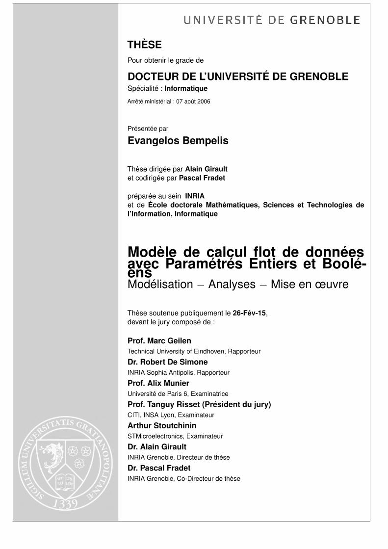
Streaming applications are characterized by large streams of data that are be-ing communicated between different computation nodes (often called actors orfilters). An example of a streaming application is shown in Figure 1. The appli-cation gets as input 3 streams (I1, I2, I3) and outputs 2 streams (O1, O2), theresult of processing of the input streams through 6 filters (F1, F2, F3, F4, F5, F6).Filter F6 has a backward connection to filter F1 forming an internal loop (feed-back).
It is evident that the requirements of streaming applications can widely vary.For applications that run on mobile devices, low power consumption is cru-cial to preserve battery life. On the contrary, medical applications need to bereliable and, in the case of remote surgery, with extremely low latency. A com-mon factor, though, is their high performance requirements, which makes theirparallel implementation a necessity.
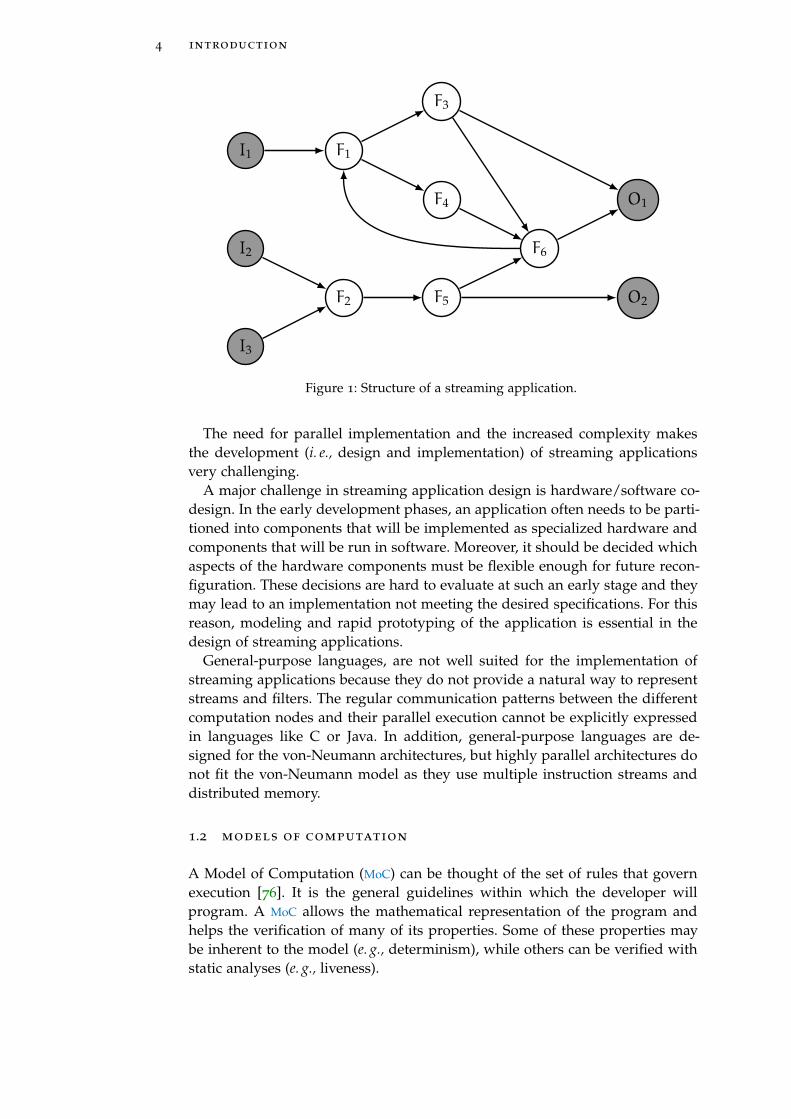
The complexity of streaming applications tends to increase, while their strictrequirements remain the same or even increase. An example is HEVC, the newestvideo coding standard, which increases the decoding complexity by 60% incomparison to its predecessor H.264 [119], while performance demands remainat the same level or even increase: for the same frame rate of 30 frames persecond and assuming their maximum resolution, 4K and 2K respectively (Fig-ure 2), the HEVC decoder needs to process 4 times the amount of data processedby H.264 in the same amount of time due to the increase in resolution.
3
4 introduction
I1
I2
I3
O1
O2
F1
F2
F3
F4
F5
F6
Figure 1: Structure of a streaming application.
The need for parallel implementation and the increased complexity makesthe development (i. e., design and implementation) of streaming applicationsvery challenging.
A major challenge in streaming application design is hardware/software co-design. In the early development phases, an application often needs to be parti-tioned into components that will be implemented as specialized hardware andcomponents that will be run in software. Moreover, it should be decided whichaspects of the hardware components must be flexible enough for future recon-figuration. These decisions are hard to evaluate at such an early stage and theymay lead to an implementation not meeting the desired specifications. For thisreason, modeling and rapid prototyping of the application is essential in thedesign of streaming applications.
General-purpose languages, are not well suited for the implementation ofstreaming applications because they do not provide a natural way to representstreams and filters. The regular communication patterns between the differentcomputation nodes and their parallel execution cannot be explicitly expressedin languages like C or Java. In addition, general-purpose languages are de-signed for the von-Neumann architectures, but highly parallel architectures donot fit the von-Neumann model as they use multiple instruction streams anddistributed memory.
1.2 models of computation
A Model of Computation (MoC) can be thought of the set of rules that governexecution [76]. It is the general guidelines within which the developer willprogram. A MoC allows the mathematical representation of the program andhelps the verification of many of its properties. Some of these properties maybe inherent to the model (e. g., determinism), while others can be verified withstatic analyses (e. g., liveness).
1.3 streaming application development with data flow MoCs 5
DVD
VCD
720p
1080p
4K
2K
Figure 2: Comparison of different video resolutions. All sizes are scaled to 16:9 ratio.
The need for rapid prototyping and deployment of massively parallel stream-ing applications has led to the development of several MoCs that facilitate designand parallel implementation. Such MoCs are meant to represent the applicationin an intuitive manner for the programmer while exposing its parallelism.
In contrast with sequential execution, where the von-Neumann model pre-vailed, in concurrent execution there still has not been a universally acceptedMoC. A plethora of MoCs that focus on parallelism has been developed, includ-ing Petri Nets [96], Kahn Process Networks [67], and Data Flow [35] and all itsvariants.
Parallelism-oriented MoCs are attractive for the prototyping of streaming ap-plications because they allow static analyses that verify various qualitative (live-ness, boundedness) and quantitative (throughput, power consumption) proper-ties of the application early in the design process. They also make parallel im-plementation easier because they provide an intuitive way to represent filtersand streams and allow the functional partitioning of an application exposingthe available parallelism and allowing modular design.
Data flow MoCs are of particular interest because they are extensively usedin industry. Lustre/Scade has been successfully used to implement flight con-trol system in Airbus planes [20] and the signaling system of the Hong-Kongsubway [82]. In addition, much of the development of data flow visual program-ming languages in the 80s was backed by industrial sources [66] resulting in thedevelopment of visual languages, such as LabView [65] which was successfullydeployed in industry, significantly reducing development time [5]. Moreover,the existence of a plethora of data flow based programming languages like Lu-cid [120], Lustre [24], Signal [9], Lucid Synchrone [25], StreamIt [117] etc., isanother indication of its widespread use.
1.3 streaming application development with data flow MoCs
Data Flow MoCs are well-suited to program streaming applications on many-core architectures. Models like Synchronous Data Flow (SDF) [78], have been

6 introduction
VariableLength
Decoding
MotionCompenation
FrameBuffer
IntraPrediction
InverseQuantization
InverseTranform + Loop
Filter
Video In
Video Out
Figure 3: General structure of a video decoder.
widely used to develop Digital Signal Processing (DSP) applications. Yet, manymodern streaming applications, such as high definition video codecs, show adynamic behavior that current MoCs cannot express.
Figure 3 shows the structure of a modern video decoder. The encoded videois first processed by the Variable Length Decoding filter, which, based on theencoding of the input, will send data to the Intra Prediction filter and to theMotion Compensation filter. As implied by its name, the amount of data sentto these filters is data-dependent. The data is processed in parallel in the twopipelines until the two streams are merged and are processed by the Loop Filter.
To capture this dynamic behavior, parametric dataflow MoCs have been in-troduced from the early 2000s, including PSDF [11], VRDF [122], SADF [116] andSPDF [43]. These models allow the amount of data exchanged between the filtersof an application to change at run-time according to the values of the manipu-lated data. This is achieved by using integer parameters.
However, not all parts of a video are encoded in the same way. For example,some frames may not use the Motion Compensation filter, or some blocks of thevideo may not be coded and may not need the inverse quantization or theinverse transform. To take advantage of this information, the topology of theapplication should be changed at run-time.
For this reason, data flow MoCs that allow the change of the graph topology atrun-time have been developed, including BDF [21] and IDF [22]. However, thesemodels lack analyzability. Moreover, current parametric data flow MoCs do notallow the topology of the application to change at run-time. Hence, there is aneed for a new data flow MoC that combines parametric exchange of data withdynamic topology changes.
Increasing the expressivity of a data flow model greatly complicates its de-ployment on a parallel architecture. Parametric exchange of data results in para-metric data dependencies, while dynamic topology changes remove and adddata dependencies at run-time. Many standard implementation techniques areincompatible with this behaviour and cannot be used. Furthermore, manualparallel implementations are hard to produce and can be error-prone.

1.4 contributions 7
Finally, static analyses of the application for properties, such as throughputand power consumption, are crucial to verify that the application meets its re-quirements. They help making design decisions early in the development pro-cess. Moreover, because of the dynamic behaviour of the application, quantitiessuch as throughput or power consumption can greatly vary at run-time. Theability to efficiently calculate the values of properties like throughput can leadto better implementations. However, existing approaches cannot be applied dueto the increased expressiveness of the MoC.
1.4 contributions
The main challenge in developing a data flow MoC lies in the trade-off betweenanalyzability and expressivity of the model. In this thesis, we propose a newdata flow MoC, the Boolean Paramatric Data Flow (BPDF) model [7], that combinesparametric data exchange between filters of the application with the ability ofdynamically changing the topology of the application. A distinguished prop-erty of BPDF is to provide static analyses for the deadlock-free and boundedexecution of the application, despite the increase in expressivity.
The increased expressivity of BPDF greatly complicates implementation. Weaddress this problem with the development of a scheduling framework for theproduction of parallel schedules for BPDF applications [8]. Our framework facil-itates the automatic production of complex parallel schedules, which are oftenhard to produce and error-prone, while preserving the boundedness and live-ness properties of the application.
Finally, we approach the problem of throughput calculation for BPDF applica-tions by finding parametric throughput expressions for the maximum through-put of a subset of BPDF graphs. An algorithm is proposed to calculate sufficientbuffer sizes for the application to operate at its maximum throughput.
The thesis is structured as follows: In Chapter 2, the current state-of-the-artdata flow MoCs are presented. Moreover, the current methods of their imple-mentation on many-core architectures are discussed. Our data flow MoC, BPDF,along with its static analyses are described in Chapter 3. Chapter 4 containsour scheduling framework and its evaluation with a modern video decoder,VC-1, expressed using BPDF. In Chapter 5, we propose a parametric throughputanalysis for BPDF. We use the analysis to express parametrically the through-put of the VC-1 decoder. Finally, the thesis is summarized in Chapter 6, wherecontributions and future work perspectives are discussed.


2D ATA F L O W M O D E L S O F C O M P U TAT I O N
Last night what we talked aboutIt made so much senseBut now the haze has ascendedIt don’t make no sense anymore
— Arctic Monkeys
Modeling is essential during development as it allows the analysis and studyof a system to be done indirectly on a model of the system rather than directlyon the system itself. Computational systems are modeled with Models of Com-putation (MoCs). These are mathematical formalisms that can be used to expresssystems.
A system captured using a MoC can be analyzed and have various properties,both qualitative (e. g., reliability) and quantitative (e. g., performance) verified.Then, the model can be used to generate code that preserves these propertieswhich in turn can be compiled into software or synthesized into hardware.This way, many aspects of the system can be explored rapidly before the actualdevelopment takes place. Moreover, specifications of the system can be verifiedand, as the human factor is limited, the procedure is less error-prone. Hence, asystem can be developed and evaluated faster, cheaper and safer.
2.1 parallel models of computation
There are many MoCs developed over the years, each one focusing on differentaspects of the system under development. For example, Finite State Machines(FSMs) focus on sequential execution and are widely used to design controlsystems while discrete event models focus on timing. In this thesis, our goal isto facilitate the development of parallel embedded systems, therefore we focuson MoCs that expose parallelism such as Petri Nets, Process Networks and DataFlow.
2.1.1 Petri Nets
Petri Nets first appeared in Carl Adam Petri dissertation “Kommunikation mit
Automaten” [Communication with automata] [96] in 1962. Petri focused on for-malizing the communication of asynchronous components of a computer sys-tem. His work drew a lot of attention and was further developed by Holt et
al. in the final report of the Information Systems Theory Project [61] in 1968.Petri Nets have been developed since, a few books summing up the advancesin the field being: Peterson’s “Petri Net Theory and the Modeling of Systems” [95]in 1981, Brams’ “Réseaux de Petri: Théorie et pratique” [19] in 1983 and Desel andEsparza’s “Free Choice Petri Nets” [36] in 1995.
9

10 data flow models of computation
p1
p2t1 t2
(a) Initial marking.
p1
p2t1 t2
(b) After t1 fires.
Figure 4: A Petri Net example.
A Petri Net is composed by two components, a net and a marking. The net isa directed bipartite multi-graph that consists of two types of nodes: places andtransitions. Places are drawn as circles and represent memory, transitions aredrawn as rectangles and represent computation units. Edges connect transitionswith places and vice versa but nodes of the same type cannot be connected. Themarking indicates the data stored currently on each place, shown as black dotsinside the places.
Each transition has a set of incoming edges connecting the transition with aset of input places. Similarly, each transition is connected with a set of output
edges with its outgoing edges. If all the input places of a transition have enoughdata the transition is called enabled. An enabled transition needs to have at leastone data token stored in its input places for each of its incoming edges.
A Petri Net executes by firing enabled transitions. First the transition con-sumes data tokens from all its input places, on token for each of the connectingedges. Then, it computes and produces one token for each outgoing edge whichis then stored in the corresponding connected place.
An example of a Petri Net is shown in Figure 4. It is composed by two tran-sitions (t1, t2) and two places (p1,p2) where p1 has one token initially storedin it. In the example of Figure 4, transition t1 has enough tokens to fire. Afterits firing, place p1 is left with no tokens but place p2 has 2 new tokens, one foreach outgoing edge of t1. Now t2 has enough tokens to fire, and so on.
Petri Net models can be used to prove system properties such as mutual ex-clusion (e. g., two transitions cannot fire in parallel), liveness (absence of dead-lock) and safety (that the system cannot reach a particular state). In Figure 4
one can easily show that t1 and t2 are mutually exclusive and that the graphwill not deadlock. However, the execution of a Petri Net is non-deterministic:when multiple processes are enabled any one may fire.
2.1.2 Process Networks
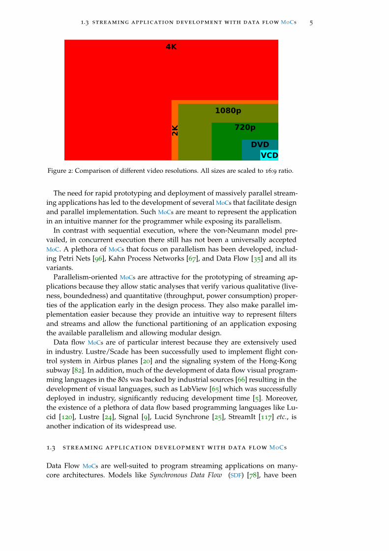
Process networks, or Kahn Process Networks (KPNs), were introduced by GillesKahn in 1974 [67]. A KPN is composed of a set of processes, interconnected withcommunication links (channels) (Figure 5). Communication links are unidirec-tional and the only way processes communicate with each other. Each processmay either be executing or may be blocked, waiting for data on one of its incom-
2.1 parallel models of computation 11
g
h0 h1
f
T1 T2
X
Y Z
Figure 5: An example of a process network with processes g,h0,h1, f and channelsT1, T2, Y,Z,X. Figure reproduced from [67].
ing communication links. A process cannot check a whether a communicationlink is empty or not. Once a process finishes execution, it produces tokens onone or many of its outgoing communication links. There is no blocking mech-anism that prohibits a process to write. Each communication link has a type(e. g., integer, boolean float etc.). The sequence of data elements on a link, calledits history, is a complete partial order.
KPNs can be formulated with a system of equations where processes are func-tions and communication links are variables. This set is reduced to a singlefixed point equation X = f(X). As the functions are continuous over completepartial orders, the equation has a unique least fixed point [67]. In this way KPNs
are deterministic: the least fixed point which depends on the histories of thecommunication links is unique therefore, the histories produced on each com-munication link are independent of the execution order of the processes. Usingthe fixed point, a KPN can be analyzed for functional verification (e. g., that theprogram will produce the desired output). Moreover, a KPN is terminating ornon-terminating depending on whether its fixed point contains finite or infinitehistories.
Although fixed point analysis gives the length of the histories of the com-munication links, it does not reason on the accumulation of data tokens whichdepends on the execution order. A KPN is strictly bounded if the accumulationof tokens on all its communication links is bounded by b for all possible exe-cution orders. A KPN can be transformed so that it is strictly bounded. To doso, feedback links are added for each communication link with b initial tokens.However, the feedback links may introduce a deadlock transforming a non-terminating program into a terminating one. Boundedness of KPNs is discussedin Parks’ thesis [93] and extended in [47].
2.1.3 Data Flow
The Data flow MoC first appeared in 1974, in a paper by Jack B. Dennis [35].The initial goal of data flow was to lift some limitations of Petri Nets and in-crease their expressiveness. Dennis’ data flow is expressive enough to expressthe source program while exposing the available parallelism.
In Dennis’ data flow, applications are expressed as directed graphs. Nodes,called actors, are function units and edges are communication links. Actors canexecute or fire once they have enough tokens on their input links, as in Petri

12 data flow models of computation
A B C3
1
2 1 3
2
actoredge
port rate
initial tokens
Figure 6: A simple SDF graph.
Nets. However, in contrast with Petri Nets, Dennis’ data flow takes into accountthe value of the data on the links. So, more specialized actors are introducedto express if-then-else structures, boolean operations, splitting and mergingof data and more. Dennis’ data flow model is very expressive though and haslimited analyzability. Hence, subsequent data flow models aimed at limiting ex-pressiveness and increasing analyzability. The most influential is SynchronousData Flow introduced in 1987 by Lee and Messerschmitt [78].
Dennis’ Data flow shares the same conceptual basis with Petri Nets but wherePetri Nets focuses on the modeling part, data flow takes a step further andallows reasoning on the type and the value of the data communicated as well asthe amount [42], a feature that was abstracted in later data flow MoCs. Moreover,data flow execution is deterministic whereas Petri Net execution is not.
In comparison with KPNs, a major difference is that processes in KPNs canbe executing by consuming data from just a subset of their inputs. In contrast,actors in data flow require data on all of their inputs. Moreover, later data flowMoCs provide analysis for properties like liveness and boundedness matchingthe analyzability of Petri Nets.
The deterministic behaviour and analyzability of data flow MoCs makes themattractive for use in streaming application development. This is also shown bythe industrial success of data flow as discussed in Section 1.2. In this thesis, wefocus on data flow MoCs, which are presented in detail in the next section.
2.2 synchronous data flow
In this section, we present Synchronous Data Flow (SDF) that makes the basisfor most of the later data flow MoCs [78]. SDF was introduced in 1987, for theimplementation of DSP applications on parallel architectures. SDF is well suitedfor DSP because of the ease of expression of such applications using the model.
In SDF, as in Dennis’ data flow, a program is expressed as a directed graph,where nodes (actors) are functional units. Edges are communication links con-necting actors implemented by First-In First-Out (FIFO) queues. The connectionof an actor with an edge is called a port. Each edge is characterized by a pro-duction (resp. consumption) rate indicating the amount of data produced (resp.
consumed) on (resp. from) the edge after the firing of the corresponding actor.As these rates also characterize the respective port, we often refer to them asport rates.

2.2 synchronous data flow 13
An SDF graph executes by firing its actors. The firing of an SDF actor has threesteps:
a. Consumption of data tokens from all its incoming edges (inputs).b. Execution of its internal, side-effect free functionc. Production of data tokens to all its outgoing edges (outputs).The number of tokens consumed or produced on an edge is defined by its
rate. An actor can fire only when all of its input edges have enough tokens(i. e., at least the number specified by each rate), in this way its execution is in-
dependent of the order the actor reads its ports. Such an actor is called fireable oreligible to fire. In SDF, all rates are constant integers, therefore known at compiletime.
2.2.1 Formal Definition
Formally, an SDF graph is defined as a 5-tuple (G, lnk, init,prd, cns) where:• G is a directed connected multigraph (A, E) (i. e., there can be more than
one edge connecting a pair of actors.) with A a set of actors, and E a setof directed edges.
• lnk : E Ñ A ˆ A associates each edge with the pair of actors that itconnects.
• init : EÑ N associates each edge with a number of initial tokens.• prd : EÑ N
˚ associates each edge with a production rate.• cns : EÑ N
˚ associates each edge with a consumption rate.For example, the simple SDF graph in Figure 6, is composed of three actors,
A = tA, B, Cu and three edges, E = tĎAB, ĎBC, ĚCAu. For convenience through-out the thesis we use the notation e = ĎXY where X and Y represent the pro-ducer and consumer of the edge. The lnk function for edge ĎAB is defined aslnk(ĎAB) = (A,B) and similarly for the rest of the edges. The init functionreturns 0 for all edges except for init(ĚCA) = 2. Finally, the prd and cns func-tions return the production and consumption rates, for example prd(ĎAB) = 3,cns(ĎAB) = 2, prd(ĎBC) = 1, cns(ĎBC) = 3, prd(ĚCA) = 2 and cns(ĚCA) = 1.
An SDF graph is characterized by its topology matrix (Γ), which is similar tothe incidence matrix from graph theory. The topology matrix has its columnsassigned to the nodes of the graph, and its rows to the edges. Each entry (i, j)of the matrix corresponds to the amount of data produced on edge i fromnode j, i. e., the corresponding port rate. Consumption of data is representedby a negative value and the absence of a link is represented by 0. If multipleedges connect two actors, the sum of the production/consumption rates is usedinstead. The topology matrix for the graph in Figure 6 is:
A B C
AB 3 -2 0
BC 0 1 -3
CA -1 0 2
The state (S) of an SDF graph is a vector indicating the number of tokensstored on each edge of the graph at a given instant. Every time an actor fires,

14 data flow models of computation
A
B
C
1
1
1
1
2
1
Figure 7: An inconsistent SDF graph.
it produces and consumes tokens altering the state of the graph. For instance,the initial state of the SDF graph in Figure 6 is Sinit = [0 0 2]. After actor A firesonce, the state of the graph becomes S 1 = [3 0 1].
2.2.2 Static Analyses
A key property of SDF is that it can be statically analyzed for consistency, bound-
edness and liveness. Analyses of these properties are formally presented in [48].These properties are crucial for embedded systems. Consistency ensures that
the graph is valid, i. e., there are no incompatible rates on the graph, openingthe way to the analyses of boundedness and liveness. Boundedness ensures that anapplication operates within bounded memory. With a known memory bound,the designer can ensure that the system has sufficient memory and allocate itstatically at the beginning of the execution of the application, greatly improvingperformance. Finally, liveness ensures the continuous operation of a system,which is generally desirable and essential for critical systems.
Consistency
To present rate consistency, we take the example of an inconsistent graph inFigure 7. As shown in the Figure 7, For each firing of actor A, actor B is enabledonce and can produce 2 tokens on ĎBC. However, actor C is also enabled onlyonce, and cannot consume both tokens that B produces. As a result, tokens willaccumulate on edge ĎBC and the graph is inconsistent. An SDF graph is consistent
if there is a set of firings that returns the graph back to its initial state. Indeed,a repetition of such a set never leads to an accumulation of tokens on any edgeand the graph is consistent.
We call such a set of firings an iteration of the graph, that is a non-empty setof actor firings that return the graph back to its initial state.
An iteration of the graph can be found by solving the so-called system of
balance equations. To return to the initial state the total production of tokens oneach edge should be to equal the corresponding consumption. Formally:
@e = ĎAB P E, D #A, #B, #A ¨ prd(e) = #B ¨ cns(e) (1)
where #A and #B are called solutions of actors A and B, respectively. They indi-cate the number of times each actor fires during the iteration.

2.2 synchronous data flow 15
We get one such Eq. (1) for each edge of the graph, ending up with a set ofbalance equations, which forms a linear system. The system can be expressedmore compactly using the topology matrix:
Γ ¨ r = 0 (2)
where r is the vector with the actor solutions. The minimum non-trivial integersolution of the system (Eq. (2)) is called the repetition vector and indicates theminimum number of times each actor needs to fire for the graph to return to itsinitial state, the minimum iteration. Although an iteration can be any multiple ofthe minimum iteration, from now on we use iteration to denote the minimumiteration, unless noted otherwise. If the system has no solution, the graph is saidto be inconsistent as it never returns to its initial state. Hence, we can formallydefine consistency:
Definition 1 (Consistency). An SDF graph is consistent iff its system of balance
equations has a non-trivial solution.
For the SDF graph in Figure 6, the balance equation for, say, the edge ĎAB is#A ¨ 3 = #B ¨ 2. The system of balance equations, using Eq. (2) is:
3 ´2 0
0 1 ´3
´1 0 2
¨
#A
#B
#C
= 0
The minimum solution is r = [2 3 1], also written r = [A2 B3 C] for betterreadability. The graph in Figure 6 is consistent, that is, there is a set of firingsthat returns the graph back to its initial state.
Boundedness
An SDF graph is bounded if it can execute in finite memory. A consistent SDF
graph is inherently bounded. By definition, there is no accumulation of tokenson any edge of the graph hence, the graph operates in bounded memory. There-fore, checking an SDF graph for boundedness, amounts to check consistency bysolving the system of balance equations. Formally:
Definition 2 (Boundedness). An SDF graph is bounded iff its system of balance
equations has a non-trivial solution.
An efficient algorithm to compute the repetition vector is presented in [6]with linear time complexity (Θ(|E|+ |A|)) in the number of actors and the num-ber of edges. The algorithm first randomly sets the solution of an actor to 1 and,as the graph is connected, it finds a solution for each actor, if it exists. Then, thealgorithm normalizes the solution to be the minimum integer solution. If thealgorithm successfully returns a repetition vector, the graph is consistent andbounded.
16 data flow models of computation
Liveness
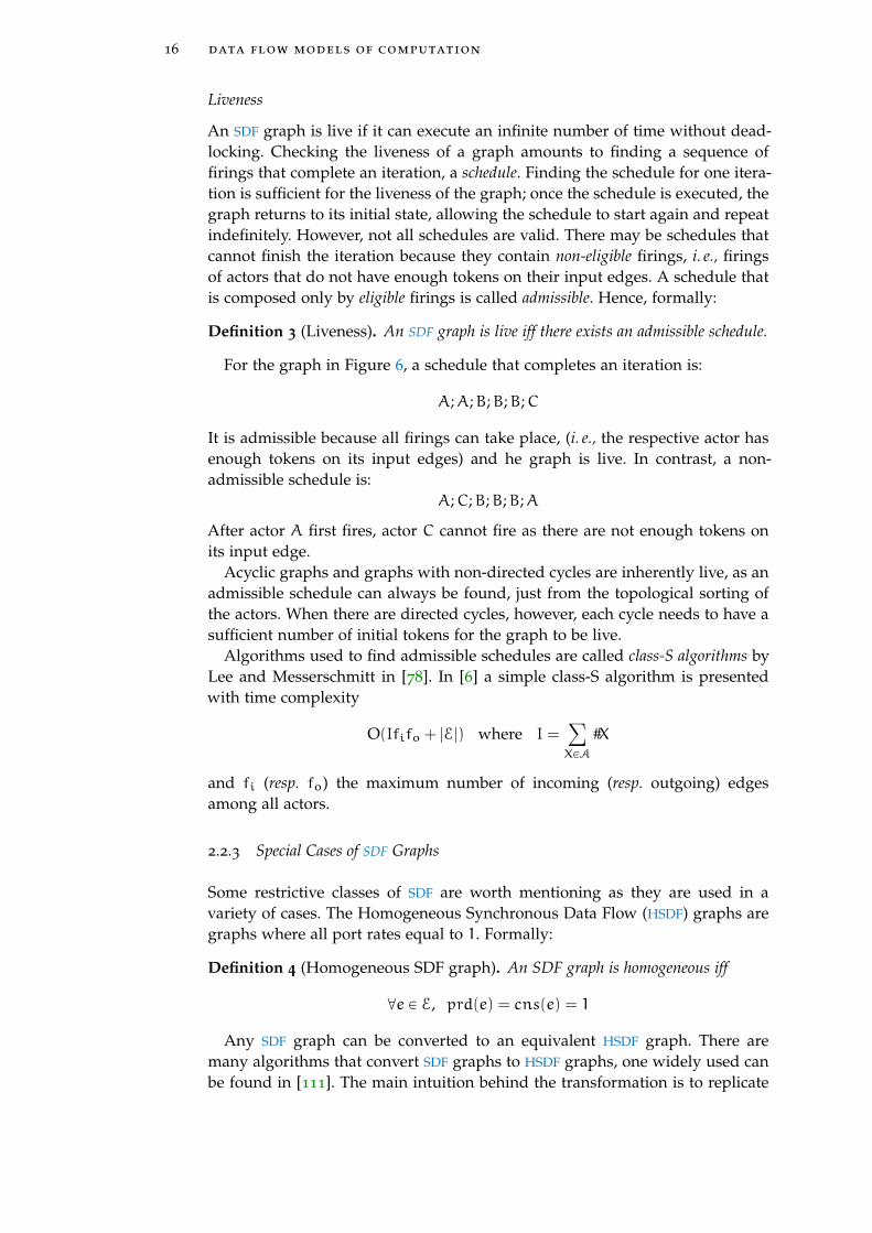
An SDF graph is live if it can execute an infinite number of time without dead-locking. Checking the liveness of a graph amounts to finding a sequence offirings that complete an iteration, a schedule. Finding the schedule for one itera-tion is sufficient for the liveness of the graph; once the schedule is executed, thegraph returns to its initial state, allowing the schedule to start again and repeatindefinitely. However, not all schedules are valid. There may be schedules thatcannot finish the iteration because they contain non-eligible firings, i. e., firingsof actors that do not have enough tokens on their input edges. A schedule thatis composed only by eligible firings is called admissible. Hence, formally:
Definition 3 (Liveness). An SDF graph is live iff there exists an admissible schedule.
For the graph in Figure 6, a schedule that completes an iteration is:
A;A;B;B;B;C
It is admissible because all firings can take place, (i. e., the respective actor hasenough tokens on its input edges) and he graph is live. In contrast, a non-admissible schedule is:
A;C;B;B;B;A
After actor A first fires, actor C cannot fire as there are not enough tokens onits input edge.
Acyclic graphs and graphs with non-directed cycles are inherently live, as anadmissible schedule can always be found, just from the topological sorting ofthe actors. When there are directed cycles, however, each cycle needs to have asufficient number of initial tokens for the graph to be live.
Algorithms used to find admissible schedules are called class-S algorithms byLee and Messerschmitt in [78]. In [6] a simple class-S algorithm is presentedwith time complexity
O(Ififo + |E|) where I =ÿ
XPA
#X
and fi (resp. fo) the maximum number of incoming (resp. outgoing) edgesamong all actors.
2.2.3 Special Cases of SDF Graphs
Some restrictive classes of SDF are worth mentioning as they are used in avariety of cases. The Homogeneous Synchronous Data Flow (HSDF) graphs aregraphs where all port rates equal to 1. Formally:
Definition 4 (Homogeneous SDF graph). An SDF graph is homogeneous iff
@e P E, prd(e) = cns(e) = 1
Any SDF graph can be converted to an equivalent HSDF graph. There aremany algorithms that convert SDF graphs to HSDF graphs, one widely used canbe found in [111]. The main intuition behind the transformation is to replicate

2.2 synchronous data flow 17
A1
A2
B1
B2
B3
C1
(a) HSDF graph.
A B C
6
3
3
2 2 6
6
(b) Normalized SDF graph.
Figure 8: The HSDF and the normalized SDF graphs of the graph in Figure 6.
each actor as many times as its solution and connect the new actors accordingto the rates of the original SDF. The resulting graph may have an exponentialincrease in size.
The resulting HSDF graph from the SDF graph in Figure 6 is shown in Fig-ure 8a. Each actor in HSDF graph corresponds to a firing in the iteration of thecorresponding actor. So, for actor A that needs to be fired twice (r = [A2 B3 C]),the HSDF has two actors (A1,A2). The edges are produces accordingly: the firstfiring of A produces 2 tokens for the first firing of B, hence the two edges be-tween A1 and B1 in the HSDF, and one token for its second firing, shown withĞA1B2.
HSDF representation is useful because it exposes all the available task paral-lelism. It has been successfully used to produce parallel schedules of SDF graphsand evaluate its throughput (see Section 2.4.3).
Another convenient class of SDF graphs is uniform or normalized SDF graphs.An SDF graph is normalized if all the ports of any given actor have the samerate. Any SDF graphs can be transformed to an equivalent normalized SDF graph.Two SDF graphs are equivalent if any schedule that is admissible for one is alsoadmissible for the other.
A simple transformation is the replacement of the rates of the ports of eachactor #A with
lcmNPA#N#A
The initial tokens should be adjusted accordingly to trigger the same number offirings of the consumer. The method is presented in detail in [86] for Weighted

18 data flow models of computation
A B(3,0,0) (1,2)
Figure 9: A CSDF graph.
Event Graphs (WEGs) which are equivalent to SDF graphs [107]. The normalizedSDF of the graph in Figure 6 is shown in Figure 8b.
2.3 extensions of synchronous data flow
This section describes the more prominent of the extensions of SDF, startingwith MoCs that are fully defined at compile-time like Cyclo-Static Data Flow [15](Section 2.3.1).
We classify the more expressive models in two categories: the ones that al-low the graph to change topology at run-time (dynamic topology models, Sec-tion 2.3.2) and the ones that allow the amount of data exchanged between actorsto change at run-time (dynamic data rate models, Section 2.3.3).
Dynamic topology models like BDF [23] and its natural expansion IDF [22]introduce specialized actors that can change the topology of the graph at run-time using boolean or integer parameters, respectively.
Dynamic data rate models use integer parameters to parameterize the amountof data communicated between the actors of a graph. Some of these models arePSDF [11], VRDF [122], SADF [116] and SPDF [43].
Many models presented below, allow actors to change their internal function-ality at run-time. In this thesis, we disregard any dynamic change of the graphthat does not affect its data flow analyses If it does not affect any of the subse-quent analyses of the model and one can safely ignore it when it comes to themodeling of the application. In the SDF MoC for example, one can assume thatthe internal functionality of the actors change at run-time. If the rates of eachport remain the same the boundedness and liveness analyses remain valid.
2.3.1 Static Models
In this section, we present Cyclo-Static Data Flow (CSDF) that extends the baseSDF model but is still fully defined statically at compile-time. CSDF was intro-duced in 1995 by Bilsen et al. [15]. It targets applications that have predictableperiodic behaviour, known at compile time. CSDF uses a series of rates that shiftcyclically instead of a single fixed rate as in SDF. This way the production andconsumption rates of an edge may change periodically. A rate can have a zerovalue, as long as the sum of the rates in a series is strictly positive.
A sample CSDF graph is shown in Figure 9. The edge ĎAB has two sets of ratesinstead of two fixed rates. Each time an actor fires, all its port rates shift to thenext value in the series. For the graph in Figure 9, the first time actor A fires, itproduces 3 tokens and the next two, 0 tokens. On the fourth firing, the rate willshift cyclically back to 3.
In [15], a consistency analysis for CSDF is given. CSDF graphs can alwaysbe translated in HSDF graphs indicating that CSDF is not more expressive than

2.3 extensions of synchronous data flow 19
SWIT
CH
FT
b
(a) SWITCH actor.
FT
SEL
EC
T
b
(b) SELECT actor.
Figure 10: BDF special actors
SDF. However, such a conversion is not always practical because it requires acombinatorial explosion of the number of actors in the resulting HSDF.
2.3.2 Dynamic Topology Models
In this section, we present two models that focus on altering the graph topol-ogy at run-time, Boolean Data Flow (BDF) and Integer Data Flow (IDF). JosephT. Buck introduced BDF in his thesis [21] as an extension of SDF that providesif-then-else functionality. BDF uses two special actors, a SWITCH and a SE-LECT actor (Figure 10). SWITCH has a single data input and two data outputs,whereas SELECT is the opposite with two data inputs and one data output.Both actors have a boolean control input that receives boolean tokens. Depend-ing on the value of the boolean tokens, SWITCH (resp. SELECT) selects theoutput (resp. input) port that is activated.
A BDF graph is analyzed like an SDF graph except for the SWITCH (resp.
SELECT) actors whose output (resp. input) ports use rates depending on theproportion of true tokens on their input boolean streams which can also beseen as the probability of a boolean token to be true. A SWITCH actor with aproportion of p true tokens in its boolean stream, will produce after n firingsn ¨ p tokens on its true output and n ¨ (1´ p) tokens on its false output. ASELECT actor will consume tokens in a similar manner.
In this way, for each separate boolean stream bi, we get a probabilistic rate pi,forming a vector ~p. The balance equations of a BDF graph include such proba-bilistic values. For the graph in Figure 11, with p1 the proportion of true tokenfor boolean stream b1 and p2 for b2, respectively, we get that a non-trivial so-lution does not exist, unless p1 = p2. BDF describes the graphs which havenon-trivial solutions for all values of ~p as strongly consistent. On the contrary,graphs that are consistent only for specific values of ~p are called weakly consis-
tent. Weakly consistent graphs cannot have guarantees (e. g., liveness, bound-edness) on their execution as it depends on the values of the tokens on theboolean steams.
BDF greatly increases SDF expressiveness. In fact, it is shown in [21] that BDF
is Turing complete and that the decision of whether a BDF application operateswithin bounded memory is undecidable as it equates to the halting problem.
BDF was extended by IDF [22]. IDF replaces BDF boolean streams with integerstreams, allowing SWITCH and SELECT actors to select one port over many,instead of just two as in BDF.

20 data flow models of computation
A
SWIT
CH
FT
FT
SEL
EC
T
B
C
D
b1 b2
2 1
1
1
1
1
1
1
1
1
1 2
Figure 11: A BDF graph.
2.3.3 Dynamic Rate Models
This section presents models that may change port rates dynamically at run-time, altering the amount of data exchanged between actors at run-time.
Parametric Synchronous Data Flow
Parameterized Synchronous Data Flow (PSDF) [11] introduces a set of parame-ters in the actor definition of SDF. These parameters may control the internalfunctionality of the actors but may also affect the data flow behaviour of thegraph as they can be used in the definition of port rates.
The PSDF MoC is organized in an hierarchical manner: each PSDF actor, unlessit is primitive, is itself a PSDF graph, a component. Each component consists ofthree subgraphs, the main data flow subgraph (body) that implements the mainfunctionality, and two auxiliary subgraphs (init and subinit), which change theparameters of the body. The links between the subgraphs of a component andits parent component can be either standard data flow links or links propagat-ing parameter values, called initflow.
The subinit subgraph changes parameters affecting only the internal function-ality of the actors in the body of the component. It can have both data flow in-puts and initflow inputs. In this way the parameters set by the subinit graph canbe data dependent and change values within the iteration of the component.
The init subgraph changes parameters that also affect data flow behaviour,such as port rates. The init graph can only have initflow inputs and its execu-tion is not data-dependent. When the parent component invokes a child, firstthe init is fired once to set its parameters and then the iteration of the subinit
and body graphs takes place. PSDF restricts the execution of the init graph likethat, to ensure that the interface between the parent component and the childremains consistent throughout an iteration of the child. In this way, PSDF re-stricts changes of parametric port rates between iterations of a component. Bothinit and subinit outputs are initflow, carrying parameter values and not part ofthe main data flow.
In Figure 12 a PSDF component is shown. The component has two sets of dataflow inputs, one to connected to the subinit graph and one to the body. There isalso an initflow carrying parameter values from the parent component. In thisexample, the body has three functions and function f2 is configured with twoparameters g and p. g changes the functionality of f1 while p sets its output rate.

2.3 extensions of synchronous data flow 21
initsubinit
body
init
set psubinit
set g
f1 f2(g) f3p
initflow
Figure 12: A PSDF component.
When the component is fired, first the init graph is fired and it sets parameterp and potentially other parameters. Finally, the rest of the graph executes as inthe SDF model, with subinit fired first to set the value for g. Within the iterationsubinit may fire multiple times to change the value of g but init fires only once.
PSDF is analyzed in the same fashion as SDF, but every possible configurationof its subgraphs needs to be taken into account. A configuration of a componentis a possible assignment of all its parameters. Once all the parameters havetaken values, the graph is reduced to an SDF graph, and all SDF analyses can beused.
Each hierarchical component is analyzed separately. A PSDF graph is con-sistent if of its components are consistent. If all possible configurations of acomponent are consistent, then the component is said to be locally synchronous,if all of them are inconsistent, the component is called locally asynchronous andin all other cases, partially locally synchronous. The exact methodology of analyz-ing a PSDF graph is not described in [11], however, an informal set of conditionsis given
a. All PSDF graphs (init,subinit,body) must be locally synchronous.b. Both init and subinit graphs need to produce exactly one token on each of
their outputs, every time they complete an iteration.c. The data flow inputs of subinit must not depend on a parameter.d. Both the inputs and the outputs of the body must not depend on a param-
eter.PSDF has been successfully used to parameterize existing DSP models. It has
been proposed as a meta-modeling technique to be used on top of various dataflow MoCs besides SDF (e. g., CSDF). However, its practical parametrization of theSDF model is not formalized enough to provide strong guarantees (bounded-ness, liveness). Moreover, the addition of the auxiliary graphs (init and subinit)increases the design complexity and makes it less intuitive. It is not clear, forinstance, when a value of a parameter is set and how often it changes.

22 data flow models of computation
A B C DTGp p
1[p] 1[p]q q
1[q] 1[q]1 1 11
Figure 13: Example of a VRDF task graph.
Variable Rate Data Flow
Variable Rate Data Flow (VRDF) [122] adds parametric rates to the original SDF
model. VRDF focuses on data flow graphs that derive from task graphs, whichare Directed Acyclic Graphs (DAGs). The VRDF graph that results from a taskgraph, also models the sizes of the buffers on the edges, resulting in a stronglyconnected graph.
VRDF restricts the usage of parametric rates either on a single actor or inpairs. When in pairs, for each actor with an output port with a parametric rate,there must be another actor with an input port with a matching parametric rate.These actor pairs must be well-parenthesized: If there is a pair using parameterp, then another pair using parameter q can be nested within the actors of thefirst pair but cannot interleave (Figure 13).
VRDF allows a parameter to take a zero value, disabling the production (resp.
consumption) of tokens on (resp. from) an edge. This is a similar behaviourwith BDF when a false boolean value deactivates the port of a SWITCH orSELECT actor. However, VRDF avoid the unboundedness problem that arises inBDF because of its requirement of parameters used in pairs as described earlier.This restriction guarantees that a consistent VRDF graph is also bounded. Tocheck the consistency of a VRDF graph, its system of balance equations of thegraph can be solved symbolically, producing a parameterized repetition vector.Parameter values propagate through extra edges between the two actors of thepair. These edges have production and consumption rates of 1 and have zeroinitial tokens.
Figure 13 gives an example of a VRDF task graph. Actors A and D use theparameterized rate p on their output and input ports respectively. Another pairof actors is nested between them, actors B and C using parameter q. Two edges(ĚAD, ĎBC) propagate the parametric values with production and consumptionrates of 1. A task graph, TG, is located between the the actors B and C. Solvingthe balance equations of the graph, we find that actors A and D have solutionsof 1, actors B and C parametric solution of p while TG has a parametric solutionequal to pq.
VRDF proposes a clean solution to increase the expressiveness of SDF withparametric rates. However, it imposes many restrictions; task graphs should beacyclic and the parametric ports come only in matching pairs.
Scenario-Aware Data Flow
Scenario-Aware Data Flow (SADF) [116] is a modification of the original SDF
model inspired by the concept of system scenarios [52]. SADF introduces a spe-cial type of actors, called detectors, and enables the use of parameters as port

2.3 extensions of synchronous data flow 23
A B C
DD1
10
3
2
2
a
a
b c
2 d
ep
q
r
Rate s1 s2a 2 1b 3 2c 1 1d 2 1e 3 1p 1 2q 3 4r 2 4
Figure 14: An SADF graph with its scenarios.
rates. Detectors, detect the current scenario the application operates in andchange the port rates of the graph accordingly.
Each detector controls a set of actors. These sets do not overlap, that is eachactor is controlled by a single detector. The detectors are connected to each actorwith a control link, a data flow edge which always has a consumption rate of1. When a detector fires, it consumes tokens from its input edges and selects ascenario. Based on the detected scenario, the detector sets its output rates thatare parameterized and produces control tokens on all output edges. When anactor fires, it first reads a token from the control link that configures the valuesof its parameters, and then waits to have sufficient tokens on its input edges.
The set of possible scenarios is finite and known at compile time. A scenariois defined by a set of values, one for each parameterized rate. A production(resp. consumption) rate of any edge can take a zero value if and only if thecorresponding consumption (resp. production) rate takes also a zero value inthe same scenario configuration.
An example of an SADF graph is given in Figure 14. For better readabilityrates of 1 are omitted. The graph is composed by 1 detector and 4 actors. ActorsB, C and D are controlled by the detector via the control links shown withdashed lines. Actor A is not controlled by any detector which means that italways operates in the same scenario – all its port rates are static. The possiblescenarios the detector may select are s1 and s2 (see Figure 14). Parametric ratesp,q and r are the production rates of the detector on the control links for eachscenario.
When the graph executes, the detector fires first choosing a scenario, say s1.The detector will produce one control token to B, three tokens to D and twotokens to C (because of the values of p,q and r in scenario s1). These tokens setthe parameters for each actor according to the scenario. For example, actor B
will execute with a = 2 and b = 3. When the control tokens are consumed, theactors wait for the detector to produce new control tokens for the next scenario.
As all scenarios are known at compile time, SADF is analyzed by analyzing allpossible SDF graphs that result from each scenario. SADF requires the solutionsof the detectors to be 1 for all scenario configurations. Hence, the detectorscannot change parameter values within an iteration. This restriction is true forthe strongly consistent SADF, for which analyses for boundedness and livenessare provided in [116]. Weakly consistent SADF graphs may support changing of

24 data flow models of computation
Aset p[1]
Bset q[p]
C2p 1 q pq
2 1
↑
↑
↓
↑
1 2p p 1
1
1 2
1 2
1 1 1 1 1 1 1
Figure 15: An SPDF graph with its parameter propagation network.
rates and topology within an iteration, but in general they are not statically ana-lyzable. When referring to the SADF model, we will always refer to the stronglyconsistent version of the model.
SADF resembles CSDF in the sense that it uses a fixed set of possible rateson each port. However, it does not impose their ordering at compile time. Incontrast with other models that use parametric rates, SADF does not require aparametric analysis as all configurations can be analyzed separately as in SDF
at compile time but this approach may be costly when the number of scenariosis large.
Schedulable Parametric Data Flow
Schedulable Parametric Data Flow (SPDF) [43] is a data flow MoC that was devel-oped to deal with dynamic applications where the rates of an actor may changewithin an iteration of the graph.
SPDF uses symbolic rates which can be products of positive integers or sym-bolic variables (parameters). The variable values are set by actors of the graphcalled modifiers. Actors that have parameters on their port rates or at their solu-tions are called users of the parameter. The parameter values are produced bythe modifiers and propagate towards all the users through an auxiliary networkof upsamplers and downsamplers.
Modifiers and users have writing and reading periods respectively. These indi-cate the number of times an actor should fire before producing / consuming anew value for a parametric rate. The writing periods are defined by an annota-tion under each modifier of the form set param[period]. The reading periodsare calculated by analyzing the graph.
Not all writing periods are acceptable. Some may cause inconsistencies andSPDF introduces safety criteria and analyses to check whether an SPDF graphsatisfies them. These analyses rely on the notion of regions formed by the usersof each parameter. SPDF demands that for a parameter to have a safe writingperiod, the subgraph defined by its region needs to complete its local iterationbefore the parameter changes value. The parameter regions may overlap, aslong as all criteria are satisfied. This is called the period safety criterion. There isalso another safety criterion but we will not go into more details here.

2.3 extensions of synchronous data flow 25
model
dynamic rates dynamic topologystatic
analysesbetween
iterations
within
iteration
between
iterations
within
iteration
sdf ˝ ˝ ˝ ˝ ‚
csdf ˝ ˝ ˝ ˝ ‚
bdf ˝ ˝ ‚ ‚ ˝
idf ˝ ˝ ‚ ‚ ˝
psdf ‚ ‚ ˝ ˝ ‚
vrdf ‚ ˝ ‚ ˝ ‚
sadf ‚ ˝ ‚ ˝ ‚
spdf ‚ ‚ ˝ ˝ ‚
Table 1: Comparison table of expressiveness and analyzability of data flow models
A sample SPDF graph is shown in Figure 15. The graph has two parameters,p and q. The modifier of p is actor A with writing period 1 and the modifierof q is actor B with writing period of p. In gray is shown the auxiliary networkfor parameter communication that propagate the parameter values. The regionof parameter p is tA, B, Cu and that of q is tB, Cu.
SPDF graphs can be statically analyzed to ensure their boundedness and live-ness. These analyses rely on the symbolic solution of the balance equations andthe satisfaction of safety criteria mentioned above. Moreover, for liveness, SPDF
checks the liveness of all directed cycles and demands that there is a directedpath from each modifier to all the users.
Compared to other parametric models, SPDF provides the maximum flexibil-ity as far as the changing of the parameter values are concerned. However, thisincreased expressivity makes scheduling SPDF applications very challenging be-cause the data dependencies are parametric and can change any time duringexecution; in contrast with other parametric models where a schedule can befound at the beginning of an iteration, in SPDF graphs parameters may changewithin the iteration, demanding a constant reevaluation of the schedule.
2.3.4 Model Comparison
To sum up, we provide Table 1 comparing the dynamic features of the modelsmentioned in the previous sections. The SDF and CSDF MoCs offer no dynamismat all. Although CSDF seemingly change both rates and topology within itsiteration, its translation to an HSDF graph indicates that it is not more expressivethat SDF.
The BDF and IDF MoCs allow the topology graph to change, however, they donot allow changes in the rates of the graph. Moreover, they lack static analysesfor boundedness and liveness.
The PSDF MoC, provides dynamic rates that may change within an iteration,i. e., a child component can change its internal rates many times during theiteration of the parent. Yet, PSDF does not provide dynamic topology and itsanalyses are not well-defined.

26 data flow models of computation
The VRDF MoC as well as the SADF MoC provide both dynamic rates anddynamic topology, however, only in-between iterations. Both have other lim-itations not captured by the table, like the restriction of the VRDF model ondynamic rates coming in matching pairs and the requirement of SADF for allscenarios to be known and analyzed at compile time.
Finally, the SPDF MoC supports rate changing in-between and within an iter-ation but not support any topology change. SPDF is analyzable but due to itscomplexity it is difficult to schedule efficiently.
Other Dataflow Models
There are many other data flow models of lesser importance. For completeness,we mention some of the more notable ones:‚ Scalable Synchronous Data Flow (SSDF) [105] adds a factor n on all the
graph rates, allowing the graph to “scale” each time it starts an iteration. Inthis way, SSDF aims to increase the efficiency of SDF by letting actors firing onlarger amounts of data.‚ Synchronous Piggybacked Data Flow (SPDF) [92] goal is to allow global
state updates without side effects. It introduces global states that allow thecontrolled, synchronous update of local states of actors throughout the graph.‚ Bounded Dynamic Data Flow (BDDF) [85] was inspired by SSDF. BDDF deals
with the limitations of SSDF like the absence of data-dependent rates or ratesthat vary in a periodic manner. BDDF allows dynamic rates as long as theamount of tokens that may accumulate on any edge is guaranteed to be boundedat compile time.‚ Cyclo-Dynamic Data Flow (CDDF) [121] extends the set of rates of the orig-
inal CSDF model to have variable lengths and variable rates each time they aretriggered.‚ DF* [29] extends the basic SDF model with data-dependent control of the
graph and non-deterministic behaviour.‚Heterochronous Data Flow (HDF) [53] enhances the SDF model by adding an
internal FSM to each actor that allow them to change port rates after each firing.HDF was developed in an effort to combine different MoCs in a single design.‚ Multi-Dimensional Synchronous Data Flow (MDSDF) [88] changes SDF rates
to have matrix dimensions, so that instead of producing and consuming tokens,actors produce and consume matrices of tokens. Such an extension makes thedevelopment of image processing application more intuitive.‚ Enable Invoke Data Flow (EIDF) [99], [101] adds a set of modes to each actor
that may change non-deterministically each time the actor is invoked. EIDF aimsto facilitate rapid prototyping of applications.‚ Core Functional Data Flow (CFDF) [99], [101] is a subset of EIDF where the
changing between actor modes is deterministic.‚ Parameterized and Interfaced Dataflow (PiMM) [37] is a parameterized data
flow model that focuses on hierarchical composition of applications. PiMM ex-tends the previous work on interface-based hierarchy of the SDF MoC [97]. It canbe seen as an evolution of the PSDF MoC.

2.4 data flow application implementation 27
scheduling
mapping ordering timing
fully dynamic run-time run-time run-time
static-assignment compile-time run-time run-time
self-timed compile-time compile-time run-time
fully static compile-time compile-time compile-time
Table 2: Mapping and scheduling taxonomy
This list of data flow models remains non-exhaustive but the models we havedescribed in this section illustrate the basic principles and motivation behinddata flow models.
2.4 data flow application implementation
Once a data flow application is developed, it consists of a set of tasks that havedata dependencies and other precedence constraints with each other. It is usu-ally represented by task graphs. Task graphs are Directed Acyclic Graphs (DAGs)where each node is a task and each edge a data dependency. The implementa-tion of such an application consists of two steps: mapping and scheduling. Sche-duling is further divided into ordering and timing. The terminology for thesesteps varies a lot in literature, e. g., sometimes mapping is called assignment.Also the whole implementation procedure is often referred to as scheduling.
Depending on when each step takes place, we get the scheduling taxonomyof Lee and Ha in [77] presented in Table 2. The order that these steps take placeis not definitive: Mapping may or may not precede scheduling. In many casesthese steps interleave to achieve optimal results.
2.4.1 Mapping
Mapping is the allocation of tasks in space. It assigns tasks to hardware elements,like processors or other specialized processing units. Mapping deals with theoptimization of the utilization of the processing elements and their communi-cation network which includes load balancing of tasks among processing el-ements, minimization of the interprocessor communication, completion timeoptimization, etc...
Load balancing aims at distributing evenly the tasks on the available process-ing elements. After load balancing takes place, if the processing elements arenot utilized at 100%, the voltage and frequency of the processing elements canbe adjusted to slow their operation and reduce their power consumption. In-
terprocessor communication needs to be taken into account as it may be very ex-pensive both time-wise and power-wise to move large amounts of data from aprocessor to another. Completion time optimization is important when it comes toheterogeneous architectures as many tasks of an application can be significantlysped up if they are allocated in the correct processing element.

28 data flow models of computation
Mapping can be seen as a bin packing problem which is known to be NP-
Complete [44]. There are many heuristics in the literature for mapping taskgraphs, some of them are First-Fit Decreasing, Next-Fit Decreasing, Best-FitDecreasing and Worst-Fit decreasing [60] typically used for tight fit in low pro-cessor availability, and First-Come First-Serve mainly used when the availableprocessors are abundant.
In the following, we consider a static mapping where each actor is mappedto a separate processing element. The motivation behind this decision is that, instreaming applications with computation intensive actors, it is a usual practiceto implement actors in hardware or use dedicated processors for a single actor.
2.4.2 Scheduling
Scheduling is the allocation of tasks in time. It consists of two steps: ordering andtiming. Ordering defines the execution order of the tasks. Timing assigns aninteger value to each task indicating the exact time at which the task will startits execution. Scheduling mainly deals with the optimization of the applicationperformance and memory utilization. It focuses on optimizing the performanceof the application (i. e., maximizing throughput and minimizing latency) as wellas its memory footprint (i. e., minimizing code size and the memory used fordata).
Parametric data flow actors usually have data-dependent execution time andhence static timing is not an option. Hence, based on the taxonomy of Table 2,we focus on self-timed scheduling.
Scheduling, just like mapping, is known to be NP-Complete [44]. There aremany scheduling techniques used in task graphs, reused from classical job-shop scheduling [26]. These techniques can also be used for SDF graphs, oncethe graph is converted into a DAG [79].
To convert an SDF graph into a DAG, first the graph is transformed into ahomogeneous SDF graph, so that each firing of an actor is also a task, andremove the edges with initial tokens. The liveness property of the original graphensures that the resulting task graph is acyclic. The technique is described indetail in [79].
Task Scheduling heuristics
Task scheduling heuristics are classified in various categories such as list sche-duling algorithms, clustering algorithms, guided random search methods andtask duplication algorithms. Here, we mention some of the heuristics developedover time.‚ List Scheduling Heuristics assign priorities to tasks based on which tasks are
ordered in a list. Some representative list scheduling algorithms are DynamicLevel Scheduling (DLS) [110], Heterogeneous Earliest Finish-Time (HEFT) [118]Mapping Heuristic (MH) [40] and Levelized-Min Time (LMT) [64].‚ Clustering Heuristics try to place heavily communicating tasks on the same
processing element, trading-off parallelism with interprocessor communication.Sample heuristics are presented in [18] and in [17].

2.4 data flow application implementation 29
‚ Task Duplication Heuristics try to utilize processor idle time to duplicate tasksand reduce the waiting time of the precedent tasks. A representative heuristicis Task Duplication based Scheduling (TDS) [103].‚ Guided Random Search Heuristics are mostly genetic algorithms used for task
mapping and scheduling. Examples are Push-Pull [71] and Problem-Space Ge-netic Algorithm (PSGA) [38].
However, these approaches are not applicable in more expressive data flowMoCs where the number of firings can be parametric.
Data Flow Scheduling
Throughout this thesis we represent schedules with strings showing the firingsof the actors. We use ‘;’ for sequential execution, ‘}’ for parallel execution, super-scripts for repetition and parenthesis for nested loops over a smaller schedule.For instance, the sequential schedule
(A3; B2)4; C2
fires actor A three times followed by actor B two times. This execution is re-peated four times before actor C is fired twice.
Sequential data flow schedules can be regarded as infinite loops over a seriesof firings completing an iteration. They are also referred to as looped schedules.So, once the previous schedule fires C twice, it starts over and repeats indef-initely. In the above schedule, each actor appears, lexically, only once. Such aschedule is called Single Appearance Schedule. Single appearance schedules areinteresting because they minimize the schedule code size (see Section 2.4.3).
Parallel scheduling of data flow graphs, involves the transformation of thegraph into its homogeneous counterpart (HSDF graph) [79]. In this way theavailable parallelism is exposed and popular techniques from task schedulingcan be used.
Consider, for example, the simple SDF graph in Figure 6, and a platform of2 processing elements (P1, P2). The equivalent HSDF graph is shown in Fig-ure 8a. Let us recall that the repetition vector of the graph is r = [A2 B3 C] andhence the set of tasks are tA1, A2, B1, B2 ,B3, C1u. For a mapping, wherefirings tA1, B1, B2, C1u are mapped on processor P1 and firings tA2, B3u onP2, we can get a self-timed parallel schedule taking into account precedenceconstraints. So, the ordering for processor P1 is (A1, B1, B2, C1) while forP2 it is (A2, B3). The precedence constraints of tasks in different processorsare B2 ą A2 , C1 ą B3. The mapping and ordering of the tasks is shown inFigure 16.
The execution on processor P1 proceeds as follows: At time instant t1 theprocessor starts execution with A1. Once A1 is finished it continues with B1.At time instant t3 the execution of B2 starts once both B1 and A2 have finishedexecution. Similarly, C1 starts executing at time instant t4. If the timing of eachtask was known, a fully static schedule would be possible.
The above schedule fires each actor as soon as it is available and is calledan As Soon As Possible (ASAP) schedule. ASAP schedules are known to providemaximal throughput [111].

30 data flow models of computation
P2 A2 B3
P1 A1 B1 B2 C1
t1 t2 t3 t4 t5
Figure 16: Mapping and ordering of the graph in Figure 6 on processors P1 and P2.
Generally, the scheduling of a data flow graph focuses on the firings of oneiteration, which is then repeated periodically. Sometimes the repetition vector ismultiplied by a factor u, the unfolding factor. In parallel schedules, this allowsthe concurrent execution of firings belonging in different iterations, enablingthe exploitation of pipelining. This gain in parallelism comes at the price of amore costly in computation and/or larger in code size schedule.
We classify the self-timed schedules of data flow graphs in three categoriesdepending on the kind of ordering decisions that take place at run-time: static,quasi-static and dynamic. A schedule is static if all ordering decisions are taken atcompile-time. A schedule is quasi-static if the only decisions taken at run-timeare decisions that depend on parameter values1. A schedule is dynamic if it isneither static nor quasi-static.
Typically, static schedules consist of series of firings and for-loops with staticboundaries. Quasi-static schedules consist of firings, for-loops with static orparametric boundaries, and if-then-else structures with conditions on param-eter values. Dynamic schedules may include computation taking into accountexternal factors and variables such as power consumption to manipulate theschedule at run-time.
The term quasi-static has taken various definitions in the literature as is pre-sented in the following sections. Our definition is compatible with most existingdefinitions. The general intuition behind the term, however, remains the same,it is a distinct class of schedules standing between purely static and dynamicschedules.
In general, static and quasi-static schedules are preferred as they often offerbetter performance due to lower scheduling overhead. However, a dynamicschedule may prove more flexible and in certain cases more efficient. Finally,there is a trade-off between the code size of the schedule and its dynamicity; astatic schedule often occupies more memory than a dynamic one as it keeps allthe precomputed information stored, instead of computing it at run-time.
2.4.3 Scheduling Optimization Criteria
Scheduling juggles with the optimization of many different, and often conflict-ing, criteria. These mainly concern the memory usage (code and buffer size) andthe performance of the application (latency, throughput).
1 In this way, quasi-static schedules make sense only for parameterized data flow MoCs.

2.4 data flow application implementation 31
A B C3 2 3 1
Figure 17: An SDF graph.
Throughput indicates the performance of an application. It is a very importantfactor, mainly in real-time applications that demand a minimum throughput tobe sustained. In some cases maintaining sufficient throughput can be crucial.Latency is a metric that measures the response time of an application. It is im-portant in applications like video conferencing, telephony and on-line gameswhere it needs to be kept to a minimum. Code size refers to the length of thecode implementing the schedule. In embedded systems memory can be sparseand minimizing the size of the schedule is sometimes crucial. Similarly, memory
used for data needs to be optimized.These criteria can be analyzed at compile-time for SDF graphs and help take
scheduling decisions. Below we discuss the underlying trades-offs betweenthese criteria when scheduling data flow graphs.
Code size
Code size affects other criteria as removing part of the schedule code will mostcertainly come in conflict with the optimization of some other aspect of theschedule.
We give below a simple example showing the trade-off between code sizeand buffer size of an SDF graph. Consider the graph in Figure 17. The repetitionvector is r = [A2 B3 C9]. One possible schedule is:
A2; B3; C9
This schedule has each actor appearing only once and is called single appearance
schedule. In this way, the code size of the schedule is minimized. However, thebuffer size needed to store data on the graph is 6 tokens on edge ĎAB andanother 9 tokens on edge ĎBC. A different schedule could be
A; B; C3; A; B; C3; B; C3
This schedule needs a buffer size of 4 tokens on edge ĎAB and a size of 3 tokenson edge ĎBC a total size of 7 tokens, a significant reduction on the 15 tokensneeded by the previous schedule. However, the code size of the schedule isnow 8 actor instances compared to the 3 instances of hte single appearanceschedule. A compromise can be found by factoring out common factors on theoriginal single appearance schedule. Factoring out 3 from actors B and C yields:
A; (B; C3)3
This schedule needs a buffer size of 6 tokens on edge ĎAB and 3 tokens on ĎBCwhile keeping the code size of the schedule the same. This trade-off is exploredin detail by Bhattacharyya and Lee in [12] and [13].

32 data flow models of computation
Buffer Size
The memory usage of the graph needs to be optimized, i. e., the buffers on theedges of the graph need to be minimized. The minimization of buffer sizes is aproblem that has two different instances, depending on whether the implemen-tation relies on a single shared memory or individual buffers.
If the edge buffers are implemented as a single shared memory, then the totalmemory usage of the graph must be minimized. This is similar to the registerallocation problem. An approach using model-checking is presented in [57].
A BτrA rB
Figure 18: A generic SDF edge with production rate rA, consumption rate rB and τ
initial tokens.
When it comes to using individual buffer between actors, then the problemis significantly different. In [6] it is proved that for any schedule, the minimumbuffer size (β) of an edge ĎAB as in Figure 18 is
β =
#rA + rB ´ g+ τ mod g if 0 ď τ ď rA + rB ´ g
τ otherwise(3)
where g = gcd(rA, rB), the greatest common divisor of the two rates. If thebuffer size is less, then there is no admissible schedule for the graph and thegraph is not live. The buffer size can be modeled with a backward edge, ĎBA,with init(ĎBA) = β´ τ as shown in Figure 19.
A B
τ
β−τ
rA rB
rA rB
Figure 19: An SDF edge with a finite buffer of size β.
However, using the minimum buffer size has an impact on throughput asit prohibits the parallel execution of the two actors sharing the edge with theminimum buffer. Therefore, there is a trade-off between the buffer size andthroughput as there is a trade-off, between buffer size and code size.
Latency
For data flow graphs, it is defined as the time delay between the beginningof the first firing of an iteration and the end of the last firing completing thesame iteration as illustrated in Figure 20. Latency is the delay between theinstance an input is taken, that is the start of an iteration of the graph, and thecorresponding output is produced.
A technique that finds schedules minimizing latency for SDF graphs is pre-sented in [50]. The technique creates a latency graph by adding one source andone sink actor on the graph. Latency is then computed based on the slowest

2.4 data flow application implementation 33
P3 A1 A2 A3 A1 A2 A3 A1 A2 A3 A1 A2 A3 · · ·
P2 B1 B1 B1 B1 · · ·
P1 C1 C2 C1 C2 C1 C2
Period
Latency
t
Figure 20: A pipelined schedule on three processors, showing the difference betweenlatency and period.
path between the two actors. The authors study the trade-off between through-put and latency showing that minimizing latency does not necessarily maxi-mize throughput and vice-versa. Moreover, the schedule minimizing latencymay not be a single appearance schedule, suggesting a trade-off between la-tency and code size.
Throughput
Throughput measures the amount of data produced per time unit. In data flow,this corresponds to the number of iterations per time unit. At first sight, it seemsthat throughput is very similar to latency. However, they are quite differentand often antagonistic. This becomes more apparent in Figure 20 where thepipelined execution of an SDF graph is considered. Throughput is the rate atwhich outputs are produced. So, if we define the period of one iteration to bethe delay between the production of two consecutive outputs, the throughputof the graph (TG) can be computed with:
TG =1
period(4)
When a data flow application is deployed on multiple processors, the through-put of an iteration can be increased arbitrarily, if the graph has no directed cy-cles, by replicating actor instances in different processors and executing themin parallel. When cycles are present, they impose a lower bound on throughputbeyond which there is no gain in performance no matter how many processorsare added.
This bound is called the iteration bound. Such a bound was first exploredin [104] and the term iteration bound for data flow applications was introducedin [91]. A parallel schedule that achieves an iteration period equal to the itera-tion bound is said to be rate-optimal. Therefore a rate-optimal schedule operatesat maximum throughput.
In SDF applications, one way to compute throughput is to convert the graphto the equivalent HSDF graph and to find the cycle with the maximum cycle mean
– the critical cycle [111]. Intuitively, the cycle with the maximum cycle mean isthe one that imposes the cyclic dependency that results in the iteration bound

34 data flow models of computation
of the graph. The cycle mean of a cycle is the sum of the execution times of theactors on the cycle, over the sum of the initial tokens on the edges of the cycle.
An algorithm calculating the MCM of a graph in O(|A||E|) time, is givenin [69]. Dasdan and Gupta [34] developed two algorithms based on a techniquethat unfolds the graph up to |A| number of times. The algorithms computethe MCM in O(|AU|+ |EU|) and Θ(|A|2 + |EU|) time respectively, where AU
and EU the are actors and the edges of the unfolded graph. However, sincethe conversion to HSDF may greatly increase the size of the graph, sometimesexponentially, this approach is not always practical.
An alternative conversion to HSDF method is proposed by Geilen [45]. Theproposed conversion produces a reduced HSDF graph (i. e., it has less actorsthan the one produced with the original algorithm). The new HSDF graph is notfunctionally equivalent to the original SDF as the approach does not aim to theexpansion of one actor per instance, but rather to a graph that has the samethroughput and latency as the original graph.
Another throughput calculation is proposed in [49], where the execution statespace of the original graph is explored until a state is visited twice. This cyclein the state space means that the execution has finished the initial transitionalbehaviour, the prologue, and reached a periodic behaviour, the steady-state. Theduration of such a period can be used to calculate throughput.
The method is formulated using (max,+) algebra [46]. A matrix GM keepsthe time delay between the production of a token in the current iteration andthe production of the equivalent token in the next iteration, characterizing thebehaviour of the graph in time. To calculate the values of the matrix, a symbolicexecution of one iteration of the graph takes place. Then, it is shown that theeigenvalue of the GM matrix corresponds to the MCM of the graph giving thethroughput value.
This new approach performs better than many algorithms that compute theMCM of HSDF graphs [49]. Another benefit of the (max,+) approach is thatit can deal with graphs demonstrating more dynamism. For instance, the tech-nique has been applied to SDF graphs with actors with parametric executiontimes in [51] and to the more expressive SADF model [32].
Throughput is antagonistic with buffer sizes. As mentioned earlier, buffersizes can be modeled as backward edges forming directed cycles. These cyclesmay impose a lower iteration bound than the iteration bound of the graph withunlimited buffer sizes, further restricting throughput. Throughput increases asbuffer sizes increase, up to an upper bound defined by the iteration bound.
Power consumption
When throughput constraints are satisfied, actors that operate faster than neededcan be slowed down to achieve a reduction in power and energy consump-tion. The most commonly used technique is Dynamic Voltage-Frequency Scal-ing (DVFS). By scaling the voltage and the frequency of a processing element,one can increase (resp. decrease) its execution speed while increasing (resp. re-ducing) its energy and power consumption.
Typically, this scaling happens in discrete pairs of Voltage-Frequency. The ad-justments of the scale can happen in various ways. They can be regular (interval-

2.4 data flow application implementation 35
based changes), they can be fixed at compile-time or event based. In the last case,the decisions are taken at run-time. Indicative control parameters that are usedto select a pair on the Voltage-Frequency scale are buffer occupancy (typicallybased on cache misses when it comes to processors) and worst-case execution
times (typically calculated at compile-time) [56]. Both metrics are indirect linksto the throughput of the application which is why the efficient calculation ofthe throughout of the application at run-time is very beneficial: it allows thescheduler to make decisions on which Voltage-Frequency pair to use for eachelement in order to minimize the energy consumption, while satisfying thethroughput constraints.
Energy-aware task scheduling has been extensively explored ([125], [56], [108],[81], [84], [74]). The typical procedure for throughput constrained applications,like real-time applications, starts with the scheduling of the tasks using EarliestDeadline First and then scaling down Voltage-Frequency on each processor toreclaim slack, a procedure called SimpleVS.
DVFS is explored for the SADF MoC, in [33]. The authors present a methodto reduce power consumption in SADF graphs. The approach starts by usingminimum frequency at the beginning of each scenario and then iteratively (ifthe iteration will not meet the deadline), changes the frequency of the criticalpath, until the throughput constraint is met.
Other Criteria
Other criteria have been considered as well. For example, Sriram and Bhat-tacharyya [111] optimize parallel SDF schedules by minimizing the synchro-nization points between processors. Also, when it comes to DVFS, lowering thefrequency increases the chances of an error. So, reliability is another “criterion”that can be optimized as shown in [1] for simple data flow graphs.
2.4.4 Scheduling Synchronous Data Flow
In the above, data flow graphs are first converted into HSDF graphs and thenscheduled reusing standard task graph scheduling techniques. However, con-verting a data flow application into an HSDF graph is not always practical andwhen it comes to more expressive models it is not even feasible.
In the SDF case, the conversion can end up in an exponential growth in thenumber of actors. This issue is addressed in [98] with a technique called clus-
tering that prevents actor explosion. The problem becomes even more evidentin CSDF applications. In the original CSDF paper [15], a scheduling techniquethat avoids the conversion to HSDF is presented. Another approach [94], usesclustering to convert the CSDF graph into a SDF graph. In both cases, some of thepotential parallelism expressed in the original CSDF graph cannot be exploited.
Various intermediate representations have been assumed to facilitate the sche-duling of SDF graphs. In [2], an interprocessor communication graph and a syn-chronization graph are used to model the self-timed execution of SDF graphs.These graphs are produced based on the mapping and ordering of the tasks.Damavandpeyma et al. [31] propose a method called Decision State Model-ing (DSM). The method models a given mapping and ordering by adding aux-

36 data flow models of computation
A
B
C
D3
1
2 2
4 2
6
1
(a) Initial SDF graph.
A
B
Z1
3
1
22
412
(b) After clustering actors C and D intoZ1.
A Z2
3
1
12
4
(c) After clustering actors Z1 and B intoZ2.
Z3
(d) After clustering actors Z2 and A intoZ3.
Figure 21: Clustering technique applied on a simple SDF graph. Eventually, the graphis clustered into a single actor
iliary actors and edges based on the decision state space of the given schedule(i. e., a state space modeling all the possible transitions between the states of theprocessors based on the given ordering). The resulting graph is significantlysmaller than those resulting from the conversion to HSDF.
Clustering is a standard scheduling technique for SDF graphs. The main prin-ciple is the replacement of a set of actors with a single actor. When the singleactor is fired, a local schedule executes, firing the clustered actors. Clusteringis usually applied iteratively until the whole graph is clustered into a singleactor. It is easy to produce the schedule of the graph afterwards, by iterativelyreplacing the execution of each actor with the execution of its clustered actors.
A simple clustering example is shown in Figure 21. The repetition vector ofthe graph is r = [A4 B6 C D2]. Initially, the actors C and D are clustered into Z1.The consumption rates of the incoming edges of Z1 are adjusted accordingly:
cns(ĚBZ1) = cns(ĚBD)ˆ #D/gcd(#C, #D) = 12
andcns(ĘAZ1) = cns(ĚAC)ˆ #C/gcd(#C, #D) = 4
The local schedule of the two clustered actors is easy found to be C;D2. Then,Z1 is clustered with B in actor Z2. Similarly, we find cns(ĘAZ2) = 12 andcns(ĘAZ2
1) = 4. The schedule of the clustered actors is B6;Z1. Finally, the two
remaining actors, A and Z2, are clustered into a single actor, Z3. The sched-ule of the clustered actors is A4;Z2. The schedule of the graph is defined byreplacing iteratively the schedules of the clusters:
Z3 Ñ A4;Z2 Ñ A4;B6;Z1 Ñ A4;B6;C;D2

2.4 data flow application implementation 37
which corresponds to a single appearance schedule.Not all sets of actors are safe to a cluster. For instance, in the second cluster-
ing step of the previous example, actors A and Z1 cannot be clustered, sincethe resulting graph would have a directed cycle that did not exist before (seeFigure 22). This artificial cycle creates a deadlock, prohibiting the constructionof an admissible schedule. The potential creation of directed cycles is the mainweakness of the clustering technique as there are graphs that cannot be clus-tered.
Z2 B12
12
4
4
Figure 22: An invalid clustering of the graph in Figure 21a that leads to the creation ofa directed cycle, making it impossible to find an admissible schedule.
Bhattacharyya describes a bottom-up approach in [14] called Acyclic Pairwise
Grouping of Adjacent Nodes (APGAN). APGAN iteratively clusters pairs of adja-cent actors until the whole graph is clustered into a single actor, similar to theclustering example we demonstrated earlier. The approach produces single ap-pearance schedules that are optimal as far as the buffer sizes are concerned,when the graph contains no initial tokens.
A different, top-down, approach is presented in [89], called Recursive Parti-tioning based on Minimum Cuts (RPMC). RPMC iteratively partitions the graphinto two subgraphs GL and GR with a schedule S
gL
L ;SgR
R where SL is the sched-ule of GL and
gL = gcdt#A|A P ALu
The algorithm continues until each subgraph is composed of a single actor.In [14], it is shown that the two approaches complement each other in the sensethat APGAN performs better with SDF with regular structures and RPMC withSDF with more irregularities.
Falk et al. [41] assume graphs consisting of both CSDF and SDF actors. Then,actors are clustered and FSMs are used to express the quasi-static schedule ofeach cluster, greatly improving performance over a dynamic implementation.
In [16], a method that produces K-periodic schedules for SDF is presented.The schedule is called K-periodic as there is a vector K that keeps the periodof execution of each actor. The paper indicates how K-periodic schedules thatachieve maximum throughput can be produced for SDF graphs. The benefit ofK-periodic schedules is that, in contrast with other approaches there is no needfor a prologue in the schedule.
Govindarajan et al. [55] present a method that minimizes the buffer require-ments while keeping the rate-optimal (i. e., maximum throughput) executionusing linear programming. Stuijk et al. [114] explores the trade-off for CSDF
graphs.

38 data flow models of computation
1
3 q
pA
B C
D
E
F
Figure 23: GST of sequential schedule (A; (B;C)p;D)3;E; Fq.
2.4.5 Scheduling more Expressive Data Flow Graphs
When it comes to graphs of more expressive MoCs, conversion to HSDF is notavailable at compile-time and it is too expensive to be used at run-time. Thatis either because of the parametric nature of the repetition vector or becauseof the dynamic topology changes. For this reason, production of schedules formore expressive MoCs is of particular interest.
Dynamic Port Rates
Lee and Ha [75][58], introduced scheduling techniques for data-dependent dataflow graphs. More specifically, they coin the term quasi-static to refer to a sched-ule statically produced at compile-time where the only computations left atrun-time are the absolutely necessary ones, i. e., a loop based on the value of aparameter unknown at compile-time. This was the prelude to what later wouldbe the basis for scheduling parameterized graphs; quasi-static scheduling isused in [10] to schedule PSDF graphs. This time the term is specified as param-
eterized looped schedules, and Bhattacharya describes a clustering technique forscheduling PSDF graphs.
In [73], Ming-Yung Ko et al. introduce a representation of sequential sched-ules called Generalized Schedule Tree (GST). These trees have leafs as actor fir-ings while parent nodes indicate the iteration count of its children. For instance,the sequential schedule
(A; (B;C)p;D)3;E; Fq
can be expressed with the GST of Figure 23.Plishker et al. [100] introduces an approach to reuse the APGAN algorithm
in more dynamic data flow graphs, producing schedules represented by GSTs.Kee et al. [70] apply the generalized schedule trees technique to optimize buffersizes of PSDF graphs.
GSTs are expanded into Scalable Schedule Trees (SSTs) in [109]. SSTs allownodes to have dynamic iteration count as well as the guarded execution of theleaves where the actor firing corresponding to the leaf can be skipped if thereare insufficient data on the actor inputs. Finally, SST features arrayed children
nodes where the children of a node are executed based on a pattern. They are

2.4 data flow application implementation 39
A B C3 1 2 4
(a) SDF graph
1 2 3 4 5 6 7 8 9 10 11 12 13 14 15 16
Slot 1 Slot 2 Slot 3 Slot 4 Slot 5 Slot 6 Slot 7 Slot 8
A A A
B B B B B B B
C C C C
(b) Slotted ASAP schedule
Figure 24: An SDF graph and its respective ASAP slotted schedule.
used to express parameterized schedules in [124]. However, SSTs as well as GSTs
are limited to sequential schedules.Apart from code and buffer size, throughput for parameterized MoCs is ex-
plored as well. In [122], minimum buffer sizes for VRDF graphs with throughputconstraints are computed.
Dynamic Topology
When it comes to dynamic topology, Buck [21] explores the generation ofbounded length sequential schedules for BDF graphs. He proposes a cluster-ing technique that achieves such schedules, However, because of the nature ofBDF, the resulting schedules may not strictly implement one iteration of thegraph and boundedness is not always guaranteed.
Parallel scheduling of BDF graphs is also addressed by Ha and Lee [58]. Theypreserve the boundary of each iteration whatever the boolean values, allowingstatic timing to be used. This is achieved by adding slack in the relevant partsof the schedule.
Ko et al. considers graphs with dynamic topology [72], and proposes a methodto produce multiple sequential schedules at compile-time that are then used atrun-time according to the current graph topology. The approach aims at thereduction of the code size schedule and the buffer sizes considering both singleand multiple appearance schedules.
Slotted Scheduling
A special type of parallel scheduling is blocked or slotted scheduling [58]. Slottedscheduling is a technique where the schedule is expressed by a sequence ofslots. In each schedule slot, a set of actors fire in parallel. A slot cannot startits execution before all the actors from the previous slot have completed theirfiring.
Slotted scheduling is sometimes preferred, as it makes it easier to expressparallel schedules. Without slots, the synchronization between processors haveto be explicitly expressed. This synchronization heavily depends on the param-eter values in graphs with parametric rates. Slotted scheduling simplifies theexpression of quasi-static schedules.

40 data flow models of computation
The main drawback of slotted scheduling is that, due to the hard synchro-nization between slots, slack may be introduced. For this reason, the main goalof slotted scheduling is to group actor firings with similar durations in the sameslot. Techniques like retiming [83], move the graph initial tokens changing thegraph data dependencies, and loop winding [54], a pipelining technique sim-ilar to functional pipelining [63], can be used to reduce the introduced slack.Moreover, the slotted schedule itself can group actors with similar executiontimes in the same slot to further reduce the slack.
Throughout the thesis, we present slotted schedules in two ways: as a set ofslot sequences for each actor, or as a single schedule stream.
Slot sequences are sequences of events that indicate whether an actor fires (F)or remains idle (E) during a slot. The events are separated by the ‘;’ operatorthat indicates sequencial execution. Indexes are used to indicate repetition ofthe same event. We use parenthesis to group parts of the sequence that mayiterate. For the slotted schedule in Figure 24b, the slot sequences of the actorsare:
A : F2
B : E;F6
C : E3; (F;E)2;F
Schedule streams are produced by merging the slot sequence of each actor to-gether, executing in parallel the events from each slot sequence in a single slot.Parallel execution is indicated with the ‘}’ operator. The merging procedureis described in detail in Appendix A.1. The merging of the schedule streamsabove yields:
A; (A}B); (B; (B}C))2;B;C;
Assuming that the timing of the actors is known, e. g., tA = 2, tB = 1 andtC = 3 time units, we get the slotted schedule shown visually in Figure 24b.We see that when actors B and C are grouped together, actor B is delayed untilthe firing of actor C is completed. For instance, it would be better to trigger the4th firing of B right after its 3rd firing in the 4th slot instead of firing it in aseparate slot, but this is not allowed by the slotted model. In this way, whenactor B is grouped in the same slot with actor C, it stands idle until the slot isfinished, introducing slack in the schedule.
2.5 summary
In this chapter, the current state-of-the-art of Models of Computation that fo-cus on parallelism was presented. Two main steps of system design have beendiscussed: modeling and implementation.
Data flow modeling has been a natural choice for the development of highlyparallel streaming applications. The intuitive design and the exposure of the un-derlying parallelism makes data flow a very attractive solution. Moreover, dataflow MoCs provide compile-time analyses for both qualitative and quantitativeproperties of the system. In this way, the development procedure becomes fasterand less error-prone, resulting in more reliable and high quality products.

2.5 summary 41
Still, new data flow MoCs are needed as current applications get more com-plex and demand increased expressiveness. Proper combination of both topo-logical and data rate dynamism has not yet been achieved in any of the existingmodels. These features are desirable in modern streaming applications that pro-cess encoded data. Based on the encoding, the amount of data as well as theparts of the application that process it may vary, as discussed in Section 1.3.
Implementation on many-core platforms is very challenging as there aremany different conflicting parameters to take into account. Many task sche-duling heuristics have been developed, and although they can be reused in lessexpressive models like SDF, they quickly become obsolete when more expres-sive models are employed. New techniques have been developed to scheduleparametric data flow graphs. However, they are limited to sequential schedules.Parallel scheduling of parametric MoCs is crucial for their efficient implementa-tion on many-core platforms.
Finally, various optimization criteria were presented. It is evident that through-put plays a prominent role in the development of an application. Most stream-ing applications have real-time constraints that are reflected on throughput con-straints. To satisfy these constraints, appropriate buffer sizes need to be selectedand power consumption needs to be fine tuned.
However, when it comes to parametric MoCs, throughput calculation at compile-time is not available since it depends on the parameters which are data-dependent.There have been some efforts to compute the throughput of more expressiveMoCs like SADF but when it comes to parametric MoCs throughput computationis still lacking.
In the following, we present a new data flow MoC that provides both topo-logical and data rate dynamism at run-time based on a combination of bothinteger and boolean parameters. The aim of the model is to increase the expres-siveness of previous MoCs, so that streaming applications, like video decoders,can be modeled more efficiently. The new MoC preserves all the static analysesthat make data flow modeling so attractive. Our new data flow MoC, BooleanParamatric Data Flow (BPDF), is presented in Chapter 3.
Furthermore, we propose a scheduling framework that can schedule dataflow MoCs on many-core platforms. The framework relies on scheduling con-straints that can derive either from the application or the designer. The con-straints are analyzed parametrically and a schedule is produced at compile-time when possible. When not, a dynamic scheduler is employed. The frame-work is presented in detail and applied to BPDF in Chapter 4.
Finally, the thesis addresses the problem of parametric throughput calcula-tion. A method of calculating throughput for MoCs with parametric rates ispresented in Chapter 5.

3B O O L E A N PA R A M E T R I C D ATA F L O W
Everything flows
— Heraclitus
Data flow Models of Computation (MoCs) are well-suited to develop stream-ing applications on many-cores. They allow the parallel development of indi-vidual parts of an application and their reuse in future applications. Data flowMoCs expose the task parallelism of the application, which is essential for an effi-cient deployment on many-core platforms.
Another feature that makes data flow modeling attractive is its static ana-
lyzability. Data flow programs can be analyzed to provide guarantees on theirexecution at compile-time. Properties like liveness and bounded execution canbe ensured. It is easy to write deadlocking applications, so liveness is impor-tant to guarantee continuous execution. Boundedness is crucial for embeddedplatforms which often have limited memory available. Knowing the amount ofmemory needed by an application at compile-time, allows its static allocation,leading to more efficient implementations.
Many streaming applications have a dynamic behavior. In order to capturethem efficiently, two main features of the underlying MoC are needed: dynamic
reconfiguration of the application topology and dynamic rates at which the vari-ous components of the application exchange data when executing.
Still, MoCs that combine both kinds of dynamic behaviour are lacking eitherin expressiveness or analyzability. To overcome this shortcoming, we propose anew MoC, called Boolean Paramatric Data Flow (BPDF), which combines integerparameters (to express dynamic rates) and boolean parameters (to express theactivation and deactivation of communication channels). Integer parameterscan change between each iteration while boolean parameters can even changewithin an iteration.
When expressiveness increases, analyzability is usually compromised. Themajor challenge with such dynamic MoCs is to guarantee liveness and bound-edness. For BPDF, we provide static analyses which ensure statically these prop-erties.
The chapter is organized as follows: In Section 3.1 we present the syntax andinformal semantics of BPDF. In Section 3.2, the static analyses are described.Then, in Section 3.3, some implementation details and subtleties raised by thedynamic features are discussed. Finally, Section 3.4 contains a comparison ofBPDF with other parametric MoCs.
3.1 boolean parametric data flow
BPDF extends SDF by allowing rates to be parametric and edges to be annotatedwith boolean conditions. This way BPDF combines dynamic port rates with dy-
43

44 boolean parametric data flow
namic graph topology. Unlike other models, BPDF strictly separates the role ofrates, which are directly linked with the graph iteration, from the role of theboolean conditions, which are linked with disabling edges and changing thegraph topology. This is achieved by restricting the integer rates of the ports tonon-zero values.
3.1.1 Parametric rates
BPDF port rates are products of positive integers or symbolic variables. They aredefined by the grammar:
R ::= k | p | R1 ¨R2
where k P N˚ and p P Pi, with Pi denoting the set of symbolic variables
standing for integer parameters.Although it is not needed for the analysis of the model, a maximal value for
each integer parameter must be specified for implementation purposes (e. g., as-signing sufficient buffer sizes). We will denote the maximum of a parameter p
as pmax. Therefore, any given parameter p varies in the interval [1..pmax].Unlike the rates of SDF graphs that are fixed at compile time, the paramet-
ric rates of a BPDF graph can change between iterations. The mechanism thatchange the integer values must guarantee that all values are set at the beginningof each iteration. The choice of such a mechanism is implementation dependentand does not interact with the analyses or compilation process.
3.1.2 Boolean conditions
Each BPDF edge is annotated by a boolean condition which deactivates the edgewhen it evaluates to false. These boolean expressions are defined by the gram-mar:
B ::= tt | ff | b | B | B1 ^B2 | B1 _B2
where tt is true, ff is false and b belongs to Pb, denoting the set of symbolicvariables standing for boolean parameters.
Each boolean parameter is modified by a single actor called its modifier. InBPDF, a modifier may change a boolean parameter within a graph iteration,using the annotation “b@π” where b is the boolean parameter to be set andπ is the period at which the boolean changes value. The period of a booleanparameter b is the exact (possibly symbolic) number of firings of its modifierbetween two successive changes. Once a new value is produced it propagatesto all the actors that need it, as discussed in Section 3.3.2.
3.1.3 Formal definition
Formally, a BPDF graph is defined as a 10-tuple:
(G,Pi,Pb, lnk, init,prd, cns,β,M,πw)
where:
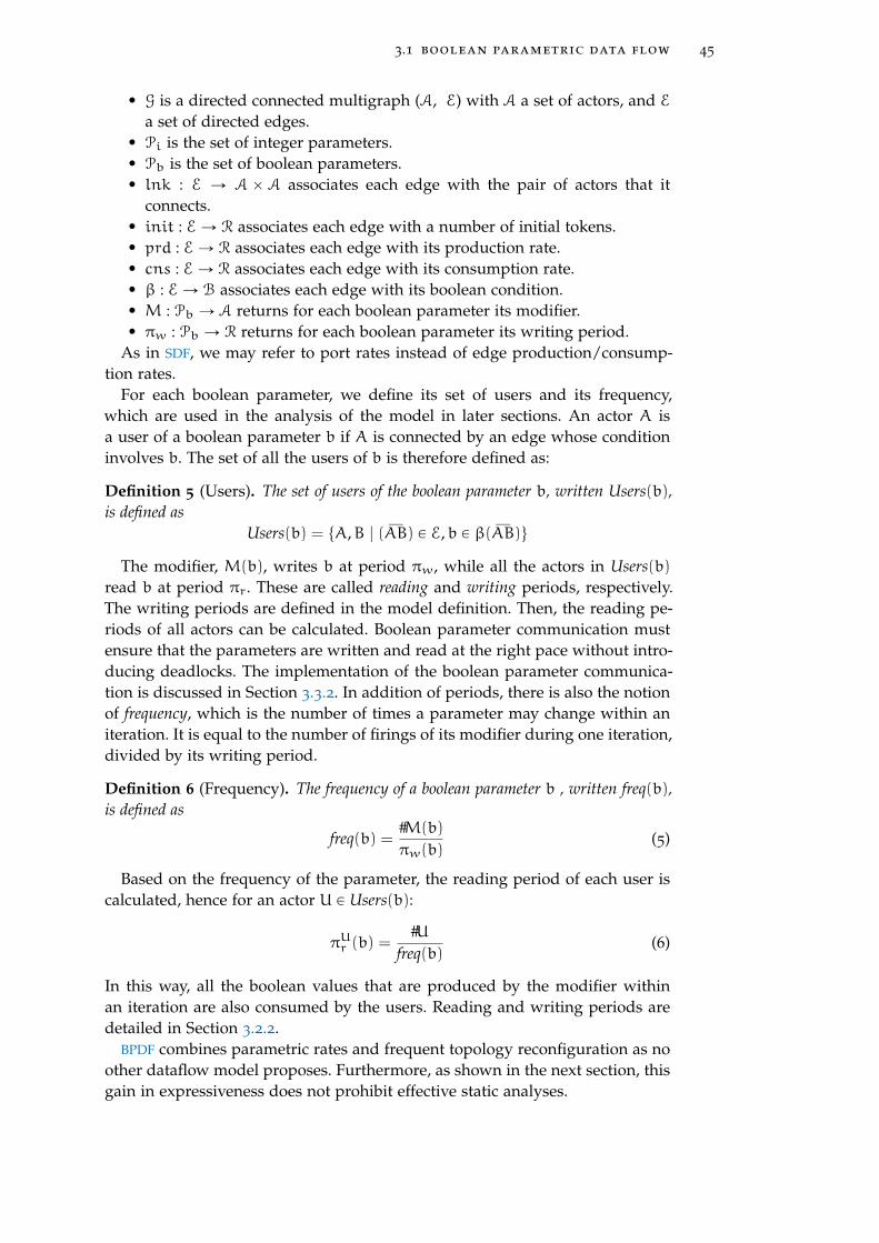
3.1 boolean parametric data flow 45
• G is a directed connected multigraph (A, E) with A a set of actors, and E
a set of directed edges.• Pi is the set of integer parameters.• Pb is the set of boolean parameters.• lnk : E Ñ A ˆ A associates each edge with the pair of actors that it
connects.• init : EÑ R associates each edge with a number of initial tokens.• prd : EÑ R associates each edge with its production rate.• cns : EÑ R associates each edge with its consumption rate.• β : EÑ B associates each edge with its boolean condition.• M : Pb Ñ A returns for each boolean parameter its modifier.• πw : Pb Ñ R returns for each boolean parameter its writing period.
As in SDF, we may refer to port rates instead of edge production/consump-tion rates.
For each boolean parameter, we define its set of users and its frequency,which are used in the analysis of the model in later sections. An actor A isa user of a boolean parameter b if A is connected by an edge whose conditioninvolves b. The set of all the users of b is therefore defined as:
Definition 5 (Users). The set of users of the boolean parameter b, written Users(b),
is defined as
Users(b) = tA,B | (ĎAB) P E,b P β(ĎAB)u
The modifier, M(b), writes b at period πw, while all the actors in Users(b)
read b at period πr. These are called reading and writing periods, respectively.The writing periods are defined in the model definition. Then, the reading pe-riods of all actors can be calculated. Boolean parameter communication mustensure that the parameters are written and read at the right pace without intro-ducing deadlocks. The implementation of the boolean parameter communica-tion is discussed in Section 3.3.2. In addition of periods, there is also the notionof frequency, which is the number of times a parameter may change within aniteration. It is equal to the number of firings of its modifier during one iteration,divided by its writing period.
Definition 6 (Frequency). The frequency of a boolean parameter b , written freq(b),
is defined as
freq(b) =#M(b)
πw(b)(5)
Based on the frequency of the parameter, the reading period of each user iscalculated, hence for an actor U P Users(b):
πUr (b) =
#Ufreq(b)
(6)
In this way, all the boolean values that are produced by the modifier withinan iteration are also consumed by the users. Reading and writing periods aredetailed in Section 3.2.2.
BPDF combines parametric rates and frequent topology reconfiguration as noother dataflow model proposes. Furthermore, as shown in the next section, thisgain in expressiveness does not prohibit effective static analyses.

46 boolean parametric data flow
A B
C
D
Ep
2 2
b
¬b
b
b@2
Figure 25: An example of a BPDF graph with an integer parameter p and boolean pa-rameter b
3.1.4 Example
Figure 25 shows a simple BPDF graph. Omitted rates and conditions are equalto 1 and tt respectively. The graph uses one parametric rate (prd(ĎAB) = p)
and a single boolean parameter, b appearing in the conditions of edges ĎBC,ĚBD and ĎCE. The modifier of b is actor B, (M(b) = B), with writing period of2, (πw(b) = 2), annotated underneath the actor with b@2. Finally, Users(b) =tB, C, D, Eu.
The repetition vector is [A2, B2p, Cp, D2p, E2p], which is computed witha symbolic variant of the classical SDF algorithm (see Section 3.2.1). With thesolution of the modifier (B) known, we can compute the frequency of booleanparameter b using Eq. (5):
freq(b) = #B/πw(b) = 2p/2 = p
which indicates that parameter b may take p different values within an itera-tion.
The conditional edges are active only when their condition (here b or b) istt. When an actor fires, it first evaluates the condition of its edges. Hence, ifthe actor is a modifier it sets all boolean values. Then, it consumes tokens onlyfrom the incoming edges with a boolean condition that evaluates to tt. Then,the actor executes its internal function and produces tokens on its outgoingedges that have a boolean condition that evaluates to tt.
This implies that a completely disconnected actor, i. e., whose edges all eval-uate to ff, still fires but does not read or write on any edge. Such a firingmay be seen as dummy firing. The propagation of boolean values still takesplace through auxiliary ports as described in Section 3.3.2. Hence, the actor cancontinue firing without consuming or producing tokens until one of booleanparameter changes and sets one of the edge conditions to tt.
With that in mind, a sample execution of the graph assuming p is set to 10
is the following: A fires and produces p = 10 tokens on edge ĎAB. Then B fires

3.2 static analyses 47
and sets the value of boolean parameter b. If b is set to tt, B does not producetokens on edge ĚBD. The reading period of D is (Eq. (6)):
πDr (b) =
#Dfreqb
=2p
p= 2
Hence, D will fire twice without consuming tokens and then will wait for thenext boolean value. B will fire a second time without changing the value of benabling C to fire once. Finally, E will consume the tokens produced by C andD.
If b is set to ff, C is disconnected and it will fire once without producingor consuming tokens before waiting for the next boolean value (πC
r (b) = 1). Dand E will fire as expected. This continues until each actor has fired a numberof times equal to its repetition count (as in SDF).
In the above, we see that BPDF execution is determinate. The output of thegraph in Figure 25 is independent of the order of execution of the enabledactors.
3.2 static analyses
Static analyses of an application are very important for embedded systems. Itprovides guarantees, and helps the development of efficient and robust appli-cations. As in SDF and some other data flow models, BPDF can be staticallyanalyzed. In this section we present how a BPDF application can be checked forconsistency, boundedness and liveness.
3.2.1 Rate Consistency
Like in SDF, rate consistency in BPDF is checked by solving a system of balanceequations. The difficulty in BPDF is that there are parametric rates and therefore,a unique integer solution cannot be found. For this, the balance equations aresolved symbolically instead, and in general, the resulting repetition vector issymbolic.
However, a BPDF graph with n boolean parameters may have up to 2n con-figurations, each one with a different system of equations, leading to multiplerepetition vectors. Furthermore, the configuration of a BPDF graph may changewithin an iteration. There is the possibility that the graph changes to a con-figuration with a different repetition vector than the previous configuration,making reasoning about an iteration very difficult.
For this reason, when checking BPDF consistency, the boolean parameters arenot taken into account. This enforces the system to be rate consistent for all pos-sible configurations of the graph. Indeed, if the system is rate consistent whenall edges are present (enabled), then it is also consistent when one or severaledges are removed (disabled). This reflects to the system of balance equationsas well because, when removing edges, the resulting system of equations willbe a subset of the original system of equations of the fully connected graph(i. e., graph with all edges active regardless the boolean values). The solution ofthe superset of equations will also be a solution of all subsets corresponding

48 boolean parametric data flow
to different configurations of the graph. In this way, the graph uses the samerepetition vector for all possible configurations.
The algorithm used to solve the system of balance equations is a general-ized version of the one used for SDF graphs in [6], using symbolic operationsinstead of integer operations. The algorithm randomly chooses one actor, setsits solution to 1, and recursively solves all other actors, according to the bal-ance equations. A normalization step is needed to yield the minimum positivesymbolic integer solution.
Checking rate consistency of all edges maybe considered too strict becauseit does not take into account the fact that some edges may not be active atthe same time (e. g., two edges annotated by b and b). On the other hand, itsimplifies the understanding and implementation since a graph has a unique(although parametric) iteration vector.
Assuming the graph in Figure 25, we arbitrarily set #B = 1. Then, due to thebalance equations we find
p ¨ #A = #B
2 ¨ #C = #B
#D = #B
#E = #D
,////.
////-
ñ
#A = 1p
#B = 1
#C = 12
#D = 1
#E = 1
To normalize we multiply all solutions with the least common multiple ofthe denominators, here we get lcm = 2p. The resulting repetition vector istherefore:
[A2 B2p Cp D2p E2p]
If the undirected version of the BPDF graph is acyclic, a solution to the balanceequations always exists. When the BPDF graph contains an undirected cycle, thegraph may be rate inconsistent. There is, however, a necessary and sufficientcondition for the existence of solutions. Each undirected cycle
X1,X2, . . . ,Xn,X1
should satisfy the following condition:
(Cycle condition) p1 ¨ p2 . . . ¨ pn = q1 ¨ q2 . . . ¨ qn (7)
where pi and qj denote respectively, the production and consumption rates ofedge (Xi,Xj). This condition enforces that the product of “output” rates of acycle should be equal to the product of “input” rates of this cycle.
Property 1 (Consistency). A BPDF graph is rate consistent iff all its undirected cycles
satisfy the cycle condition (Eq. (7)).
Proof. To prove Property 1, we consider a cycle
X1p1 q2
X2p2
. . .qn
Xnpn q1
X1
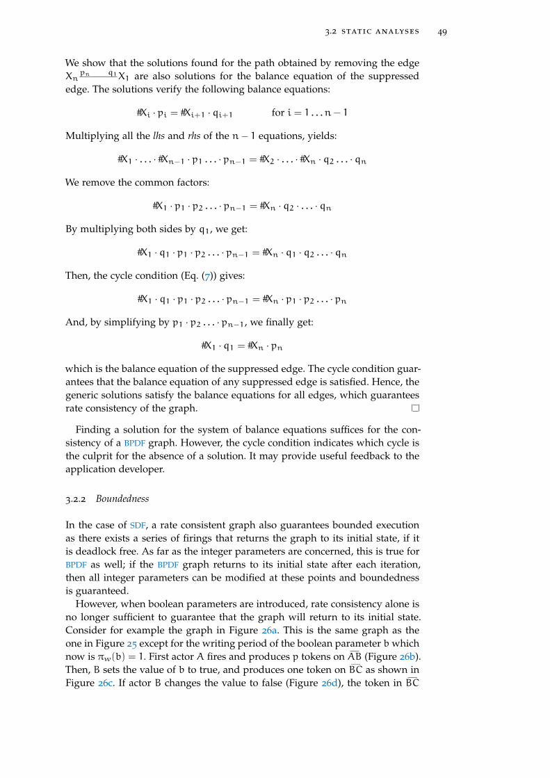
3.2 static analyses 49
We show that the solutions found for the path obtained by removing the edgeXn
pn q1X1 are also solutions for the balance equation of the suppressededge. The solutions verify the following balance equations:
#Xi ¨ pi = #Xi+1 ¨ qi+1 for i = 1 . . . n´ 1
Multiplying all the lhs and rhs of the n´ 1 equations, yields:
#X1 ¨ . . . ¨ #Xn´1 ¨ p1 . . . ¨ pn´1 = #X2 ¨ . . . ¨ #Xn ¨ q2 . . . ¨ qn
We remove the common factors:
#X1 ¨ p1 ¨ p2 . . . ¨ pn´1 = #Xn ¨ q2 ¨ . . . ¨ qn
By multiplying both sides by q1, we get:
#X1 ¨ q1 ¨ p1 ¨ p2 . . . ¨ pn´1 = #Xn ¨ q1 ¨ q2 . . . ¨ qn
Then, the cycle condition (Eq. (7)) gives:
#X1 ¨ q1 ¨ p1 ¨ p2 . . . ¨ pn´1 = #Xn ¨ p1 ¨ p2 . . . ¨ pn
And, by simplifying by p1 ¨ p2 . . . ¨ pn´1, we finally get:
#X1 ¨ q1 = #Xn ¨ pn
which is the balance equation of the suppressed edge. The cycle condition guar-antees that the balance equation of any suppressed edge is satisfied. Hence, thegeneric solutions satisfy the balance equations for all edges, which guaranteesrate consistency of the graph.
Finding a solution for the system of balance equations suffices for the con-sistency of a BPDF graph. However, the cycle condition indicates which cycle isthe culprit for the absence of a solution. It may provide useful feedback to theapplication developer.
3.2.2 Boundedness
In the case of SDF, a rate consistent graph also guarantees bounded executionas there exists a series of firings that returns the graph to its initial state, if itis deadlock free. As far as the integer parameters are concerned, this is true forBPDF as well; if the BPDF graph returns to its initial state after each iteration,then all integer parameters can be modified at these points and boundednessis guaranteed.
However, when boolean parameters are introduced, rate consistency alone isno longer sufficient to guarantee that the graph will return to its initial state.Consider for example the graph in Figure 26a. This is the same graph as theone in Figure 25 except for the writing period of the boolean parameter b whichnow is πw(b) = 1. First actor A fires and produces p tokens on ĎAB (Figure 26b).Then, B sets the value of b to true, and produces one token on ĎBC as shown inFigure 26c. If actor B changes the value to false (Figure 26d), the token in ĎBC
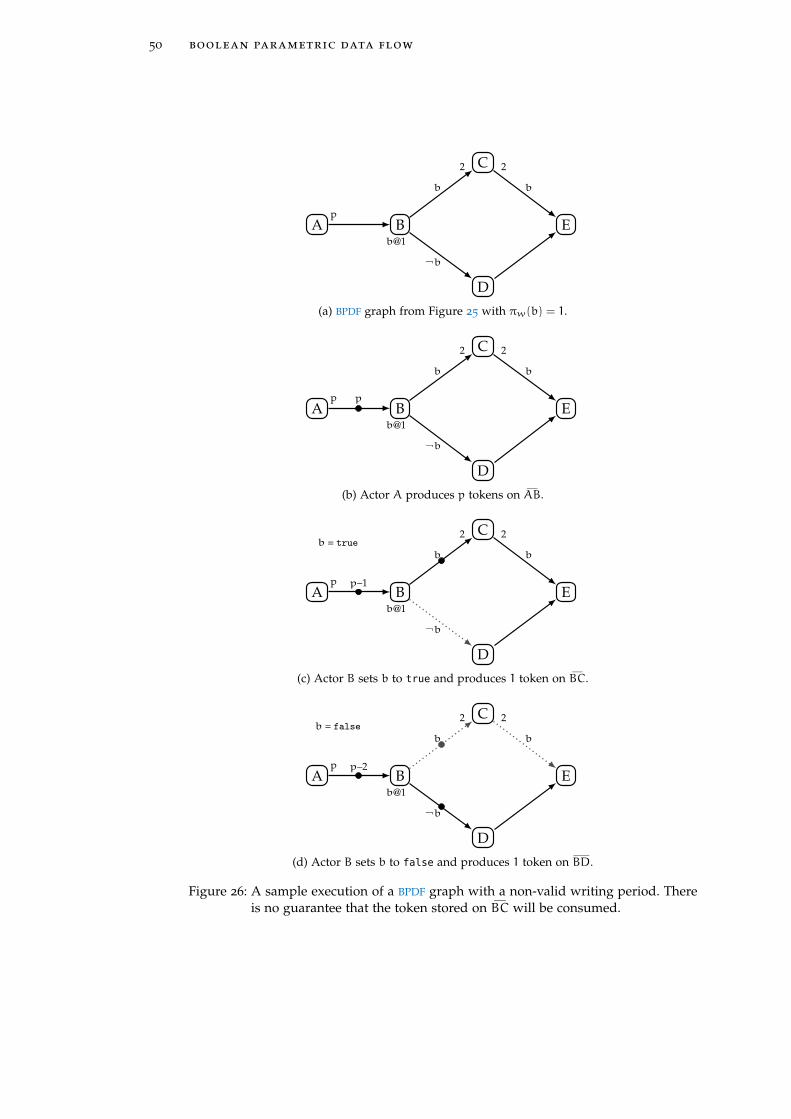
50 boolean parametric data flow
A B
C
D
Ep
2 2
b
¬b
b
b@1
(a) BPDF graph from Figure 25 with πw(b) = 1.
A B
C
D
Ep
2 2
b
¬b
b
b@1
p
(b) Actor A produces p tokens on ĎAB.
A B
C
D
Ep
2 2
b
¬b
b
b@1
p–1
b = true
(c) Actor B sets b to true and produces 1 token on ĎBC.
A B
C
D
Ep
2 2
b
¬b
b
b@1
p–2
b = false
(d) Actor B sets b to false and produces 1 token on ĚBD.
Figure 26: A sample execution of a BPDF graph with a non-valid writing period. Thereis no guarantee that the token stored on ĎBC will be consumed.

3.2 static analyses 51
will not be consumed by actor C and there is no guarantee that b will take asecond true value. With one token stored on ĎBC the graph is unable to returnto its initial state and its iteration is compromised. Boundedness and livenessare no longer guaranteed.
It is clear that not all periods are safe and their consistency must be checked.The criterion ensuring that parameter modification periods are safe relies onthe notions of regions and local iterations.
Definition 7 (Region). The region of a boolean parameter b, noted R(b), is defined as:
R(b) = M(b)YUsers(b)
The region of a boolean parameter is the set containing its modifier and allits users. For example, the region of b in Figure 25 (same as in Figure 26a) isR(b) = tB, C, D, Eu.
Definition 8 (Local solutions). The local solution of an actor Xi in a subset of actors
L = tX1, . . . ,Xnu, written #LXi, is defined as:
#LXi =#Xi
gcd(#X1, . . . , #Xn)
The solutions of the system of balance equations are called global solutions
because they define the number of firings for the iteration of the whole graph.Given a subset of actors in a graph, we can extract a subgraph and accordinglya new, smaller system of balance equations. By solving this system, a poten-tially different solution is found for each actor, indicating the number of firingsneeded for the subgraph to return to its initial state. These solutions are calledlocal solutions and they denote a nested iteration. We call the iteration of the sub-graph a local iteration to differentiate it from the iteration of the graph calledglobal iteration.
Definition 9 (Period Safety). A BPDF graph is period safe if and only if for each
boolean parameter b P Pb and each actor X P R(b),
Dk P N˚, #X = k ¨ freq(b)
The factor k is the reading (or writing) period of b for X.
Intuitively, the period safety criterion states that a parameter can be modifiedat most once per local iteration of its region. For the graph in Figure 25, b
can be changed after each iteration of the subgraph formed by the actors inR(b) = tB,C,D,Eu. We find that the iteration of the subgraph is (B2 C D2 E2),hence b can change after every 2 firings of B. This formalizes why the writingperiod of 2 in Figure 25 is safe and why the period of 1 in Figure 26a is not.
Another way to obtain the local iteration of a region is by factorizing theglobal solutions of the actors in the region of the boolean parameter by theirgreatest common divisor. Here, the global iteration is A2 B2p Cp D2p E2p. Thegreatest common divisor of the solutions of the actors in R(b) is p. Factorizingby p yields A2 (B2 C D2 E2)p, giving us the local iteration in the parenthesis.Therefore, actor B can write a new boolean value every 2 firings, while actorsC,D,E read a new value after 1, 2, and 2 firings, respectively.

52 boolean parametric data flow
However, local iterations can only be defined when the number of firings ofeach actor in the region of a parameter b is a multiple of the frequency of b.This property is called period safety.
Period safety ensures that, during a local iteration of a region of a givenboolean parameter, the number of tokens produced on any edge of this regionequals the number of tokens consumed from this edge. It is ensured by a simplesyntactic check on BPDF graphs.
In Figure 25, R(b) = tB,C,D,Eu, freq(b) = #M(b)/πw(b) = p, and the rep-etition vector is [A2 B2p Cp D2p E2p]. Each solution of the actors of R(b) isa multiple of the frequency p. The annotation b@2 of B is thus period safe. Incontrast, the graph in Figure 26a uses a writing period πw(b) = 1. This gives anew frequency of freq(b) = #M(b)/πw(b) = 2p. However, the solution of actorC is not a multiple of freq(b) so, πw(b) = 1 is not a safe period.
Property 2 (Boundedness). A rate consistent and period safe BPDF graph returns to
its initial state at the end of its iteration.
Proof. To prove Property 2, we consider an arbitrary edge (Figure 27), and showthat, during an iteration, X produces the same number of tokens that Y con-sumes. In this way, the edge returns to its initial state after an iteration. Whenall edges return to their initial state, so does the graph.
X Yx yf(b1,b2, · · · ,bn)
Figure 27: An arbitrary BPDF edge.
The condition f(b1, ¨ ¨ ¨ ,bn) is a boolean condition depending on n booleanparameters b1,b2, ...,bn. Due to period safety, for each bi P tb1, ¨ ¨ ¨ ,bnu wehave:
Dki, ℓi P N˚, #X = ki ¨ freq(bi) and #Y = ℓi ¨ freq(bi) (8)
By rate consistency, we also have
#X ¨ x = #Y ¨ y
Therefore, for each bi P tb1, ¨ ¨ ¨ ,bnu:
ki ¨ x = ℓi ¨ y (9)
When actor X (resp. Y) is fired, it produces x (resp. consumes y) tokens iff(b1, ¨ ¨ ¨ ,bn) and 0 otherwise. We write that X produces prod(b1, ¨ ¨ ¨ ,bn) andY consumes cons(b1, ¨ ¨ ¨ ,bn) with
prod(b1, ¨ ¨ ¨ ,bn) = if f(b1, ¨ ¨ ¨ ,bn) then x else 0
cons(b1, ¨ ¨ ¨ ,bn) = if f(b1, ¨ ¨ ¨ ,bn) then y else 0
During an iteration, there will be freq(bi) (potentially different) values of booleanbi. We note these values as the vector ~bi. Let Ò be the upsampling operator onvectors defined as
[x1, . . . , xn] Ò k = [x1, ¨ ¨ ¨ , x1loooomoooonk
, ¨ ¨ ¨ , xn, ¨ ¨ ¨ , xnlooooomooooonk
]
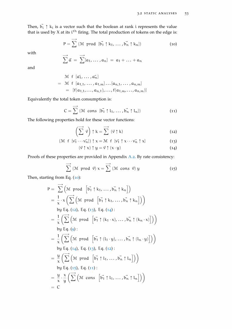
3.2 static analyses 53
Then, ~bi Ò ki is a vector such that the boolean at rank i represents the valuethat is used by X at its ith firing. The total production of tokens on the edge is:
P =
−Ñÿ(M prod [ ~b1 Ò k1, . . . , ~bn Ò kn]) (10)
with−Ñÿ
~a =
−Ñÿ[a1, . . . ,an] = a1 + . . . + an
and
M f [ ~a1, . . . , ~an]
= M f [a1,1, . . . ,a1,m] . . . [an,1, . . . ,an,m]
= [f(a1,1, . . . ,an,1), . . . , f(a1,m, . . . ,an,m)]
Equivalently the total token consumption is:
C =
−Ñÿ(M cons [ ~b1 Ò l1, . . . , ~bn Ò ln]) (11)
The following properties hold for these vector functions:(
−Ñÿ~v
)
Ò k =
−Ñÿ(~v Ò k) (12)
(M f [ ~v1 ¨ ¨ ¨ ~vn]) Ò x = M f [ ~v1 Ò x ¨ ¨ ¨ ~vn Ò x] (13)
(~v Ò x) Ò y = ~v Ò (x ¨ y) (14)
Proofs of these properties are provided in Appendix A.2. By rate consistency:
−Ñÿ(M prod ~v) x =
−Ñÿ(M cons ~v) y (15)
Then, starting from Eq. (10):
P =
−Ñÿ (
M prod[
~b1 Ò k1, . . . , ~bn Ò kn
])
=1
x¨ x
(
−Ñÿ (
M prod[
~b1 Ò k1, . . . , ~bn Ò kn
])
)
by Eq. (12), Eq. (13), Eq. (14) :
=1
x
(
−Ñÿ (
M prod[
~b1 Ò (k1 ¨ x), . . . , ~bn Ò (kn ¨ x)])
)
by Eq. (9) :
=1
x
(
−Ñÿ (
M prod[
~b1 Ò (l1 ¨ y), . . . , ~bn Ò (ln ¨ y)])
)
by Eq. (14), Eq. (13), Eq. (12) :
=y
x
(
−Ñÿ (
M prod[
~b1 Ò l1, . . . , ~bn Ò ln
])
)
by Eq. (15), Eq. (11) :
=y
x¨x
y
(
−Ñÿ (
M cons[
~b1 Ò l1, . . . , ~bn Ò ln
])
)
= C

54 boolean parametric data flow
Therefore, for any edge and any successive boolean values, the number of pro-duced tokens is equal the number of consumed tokens in an iteration. Hence,all edges return to their initial state after one iteration and therefore, so doesthe graph.
Rate consistency and period safety are crucial to ensure this property. How-ever, we assume that actors can be fired in the right order to respect dataflowand parameter communication constraints. This holds only when the graph islive and the next section shows how liveness is checked.
3.2.3 Liveness
In SDF, checking liveness is performed by finding a schedule for a basic iteration.Since each actor must be fired a fixed number of times in each iteration, thiscan be done by an exhaustive search. A class of algorithms that finds schedulesfor SDF is class-S algorithms discussed in Section 2.2.2. The situation is morecomplex in BPDF for two reasons:
• First, boolean parameters have to be communicated within the iteration,from modifiers to users. This introduces new constraints between firingsof modifiers and users which may introduce deadlocks.
• Second, actors may have to be fired a parametric number of times duringan iteration. Finding a schedule may, in general, involve some inductivereasoning.
Boolean Parameter Communication
Boolean parameter communication is implemented by adding new edges to theoriginal BPDF graph. For each parameter boolean b, we add between its modifierM = M(b) and each user U P Users(b), an edge e = ĚMU, with prd(e) = u andcns(e) = m, with u and m being the local solutions of U and M in the regionof b:
u = #R(b)U and m = #R(b)M
In other words, M and U occur as (. . . Mm . . . Uu . . .) in the local iteration cor-responding to the region of b. It is easy to see that the solutions of the balanceequations of the original graph are also valid for these new edges. During alocal iteration, M will produce m ¨ u copies of the value of b, which will all beread by U during this local iteration. The sample BPDF graph from Figure 25
with its additional boolean propagation edges is shown in Figure 28. In Sec-tion 3.3.2 we present a refinement of this implementation, which sends onlyone copy for each new boolean value.
This implementation allows modifiers to change the value of a boolean pa-rameter even when the previously sent value has not been read. In this context,the effect of boolean parameters might be better described as disabling portsinstead of edges. Indeed, at a given instant the input and output ports of anedge may be in a different state (i. e., one enabled and one disabled).
For example, in Figure 28, actor B may fire all 2p firings and produce allp boolean values for parameter b on the boolean propagation edges, beforeactors C,D and E start executing. When these actors execute they will enable

3.2 static analyses 55
A B
C
D
Ep
2 2
b
¬b
b
b@2
2
Figure 28: BPDF graph with its boolean propagation edges (dashed edges).
and disable their input ports depending on the boolean value that they readfrom their boolean propagation edges. The safety period criterion guaranteeseach actor will use the correct boolean values and the all tokens produced willalso be consumed.
The BPDF MoC ensures that the same number of tokens will be produced andconsumed on each edge during an iteration (see Property 2).
The newly added communication edges may introduce new cycles in thegraph, and subsequently deadlocks. As a consequence, liveness analysis mustbe performed on the BPDF graph augmented with all its communication edges.The augmented graph includes all possible constraints. Therefore, if it is live,all resulting subgraphs with less edges (and thus less constraints) are live aswell.
Acyclic Graphs and Saturated Edges
Acyclic BPDF graphs are always live. In such case, the topological order of theDAG defines a single appearance schedule [6]. The graph in Figure 28 is acyclicand we easily find the schedule
A2;B2p;Cp;D2p;E2p
which shows that the graph is live.Moreover, graphs where each cycle has at least one saturated edge is live. An
edge is said to be saturated if it contains enough initial tokens for its consumerX to fire #X times. Since this edge has at least the total number of tokens con-sumed by X in a complete iteration, it does not introduce any constraints andcan be ignored. If each cycle has a saturated edge, then the graph can be con-sidered as acyclic (by removing this saturated edge) and therefore live. Thesingle appearance schedule corresponding to the topological order of the DAG
obtained by removing all the saturated edges is also a schedule for the originalgraph.

56 boolean parametric data flow
A B C2p
p
(a)
A B C2p
p
(b)
A B Cb
¬bb@1
(c)
Figure 29: Various cases of live BPDF graphs.
Parametric SDF-like Liveness Checking
When there are cycles without any saturated edge, we adapt the approach takenin SDF. Checking the liveness of cyclic SDF graphs is done by computing aniteration by abstract execution. Since the total number of firings is fixed, allpossible orderings of firings can be tested. We adapt this approach to BPDF by
• ignoring booleans (all edges are assumed to be always enabled);• testing only schedules where each s consecutive firings of an actor A
represents an integer fractional of its solution, i. e., Dk P N˚, #A = k ¨ s
Ignoring boolean conditions is safe since it maximizes constraints. If a sched-ule is found by assuming that all conditional edges are enabled, it will also bevalid if some of these edges are disabled. In this way, a global schedule is found,admissible for all possible configurations of the graph.
By considering only occurrences of the form As with #A = k ¨ s, we boundthe number of such occurrences. For instance, if #A = α ¨ p, then at most α
occurrences will be considered in the abstract execution. In other words, if anactor needs to be fired a parametric number of times, only parametric numberof firings will be considered. With this constraint, the liveness algorithm ofSDF can be reused. We refer to this algorithm as Parametric SDF-like LivenessChecking (PSLC).
The PSLC algorithm is shown in Alg. 1. It is composed by a while loop overthe firings in the repetition vector and a for loop over the set of actors. Eachtime the algorithm checks whether an actor has firings left, if it does, the al-gorithm tries to fire it. If the firings left are parametric the algorithm tries tofire the actor a parametric number of times. If the actor can fire the requirednumber of firings it is added to the schedule and both the graph status and therepetition vector are updated. The algorithm continues till a repetition vectorworth of firings are scheduled or if no firing was added to the schedule afterthe end of the for-loop. This indicates that there is a deadlock.
For instance, the graph in Figure 29a has a repetition vector of [A B2p C2p].The sole cycle C = tB, Cu of the graph has no saturated edges; to be saturatedthe edge ĎCB would need 2p tokens instead of only p tokens. Still, the PSLC
algorithm finds the schedule A; (Bp;Cp)2 and this graph is live.Yet, there are cycles for which this approach is not sufficient. There are
graphs where actors with parametric solutions need to be considered in non-parametric occurrences. Consider, for example, the graph of Figure 29b. Its
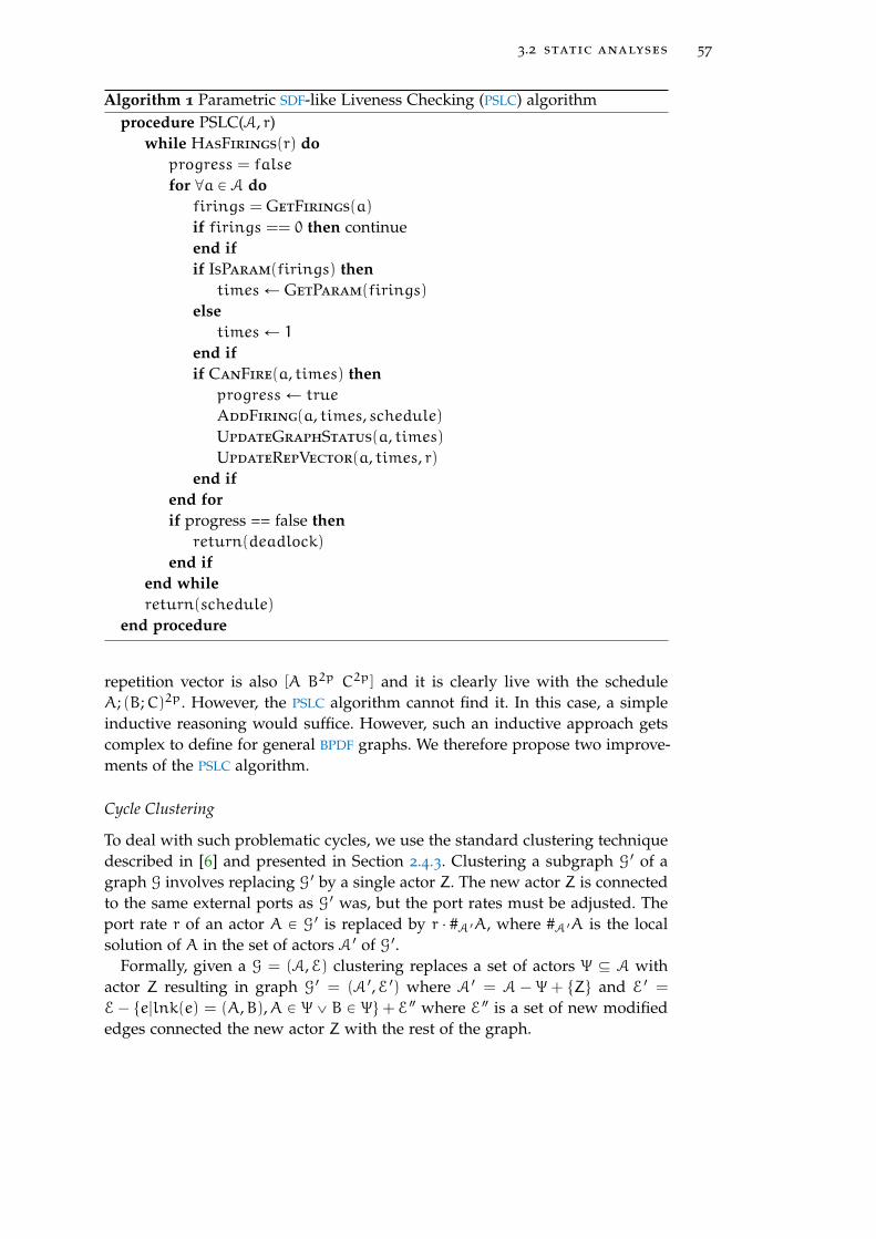
3.2 static analyses 57
Algorithm 1 Parametric SDF-like Liveness Checking (PSLC) algorithmprocedure PSLC(A, r)
while HasFirings(r) do
progress = false
for @a P A do
firings = GetFirings(a)
if firings == 0 then continueend if
if IsParam(firings) then
timesÐ GetParam(firings)
else
timesÐ 1
end if
if CanFire(a, times) then
progressÐ true
AddFiring(a, times, schedule)UpdateGraphStatus(a, times)
UpdateRepVector(a, times, r)end if
end for
if progress == false then
return(deadlock)
end if
end while
return(schedule)
end procedure
repetition vector is also [A B2p C2p] and it is clearly live with the scheduleA; (B;C)2p. However, the PSLC algorithm cannot find it. In this case, a simpleinductive reasoning would suffice. However, such an inductive approach getscomplex to define for general BPDF graphs. We therefore propose two improve-ments of the PSLC algorithm.
Cycle Clustering
To deal with such problematic cycles, we use the standard clustering techniquedescribed in [6] and presented in Section 2.4.3. Clustering a subgraph G 1 of agraph G involves replacing G 1 by a single actor Z. The new actor Z is connectedto the same external ports as G 1 was, but the port rates must be adjusted. Theport rate r of an actor A P G 1 is replaced by r ¨ #A 1A, where #A 1A is the localsolution of A in the set of actors A 1 of G 1.
Formally, given a G = (A,E) clustering replaces a set of actors Ψ Ď A withactor Z resulting in graph G 1 = (A 1,E 1) where A 1 = A ´ Ψ + tZu and E 1 =
E´ te|lnk(e) = (A,B),A P Ψ_ B P Ψu+ E2 where E2 is a set of new modifiededges connected the new actor Z with the rest of the graph.

58 boolean parametric data flow
So, for each e = ĎAB P E with A P Ψ and B R Ψ we get an edge e 1 = ĎZB withthe same initial tokens and consumption rate but with
prd(e 1) = prd(e)ˆ #A/#ΨA
with #ΨA = #A/gcd(t#X|X P Ψu). Similarly, we get edges with Z as consumer.for each e = ĎAB P E with A R Ψ and B P Ψ we get an edge e 1 = ĎAZ with thesame initial token and production rate but with
cns(e 1) = cns(e)ˆ #B/#ΨB
In general, clustering arbitrary subgraphs may introduce cycles. Here, by clus-tering only cycles, we avoid introducing new ones.
For each cycle C = X1, . . . ,Xn, our PSLC algorithm finds a local schedule.If the fraction of the total number of firings of each actor over its number offirings in this local schedule is parametric, the cycle is clustered into a newactor Z. The rate r of each port of an actor Xi connected to the rest of the graphis replaced by r ¨ #CXi. It follows that a firing of Z corresponds to the firingsXk1
1 , . . . ,Xknn with ki = #CXi.
For instance, the local schedule for the cycle of the graph of Figure 29b isB;C. The fraction of the total number of firings over the number of firings inthe local schedule is parametric for each actor (2p1 = 2p in both cases). Thecycle is clustered into a new actor Z to get the new graph in Figure 30.
A Z2p
b@1
Figure 30: Actors B and C from Figure 29b clustered into actor Z.
The PSLC algorithm now finds the schedule A;Z2p which corresponds toA; (B;C)2p for the original graph, which is therefore correctly found to be live.
False Cycles
A final refinement is needed to take into account false cycles. For instance, theprevious algorithm would fail to find a schedule for the cycle in Figure 29csince it does not have any initial tokens. However, it is clear that one of its twoedges is always disabled; in other words, this cycle is false. We also deal withthis issue by using clustering.
False cycles are detected using a truth table for all the conditions of the cy-cle or using an SMT solver. If, for each combination of values of the booleanparameters, at least one condition is false, then the cycle is false. The subgraphforming cycle C can be clustered, as for each set of values of the boolean pa-rameters, a – potentially different – schedule can always be found because in allcases the subgraph is acyclic (one edge of the cycle is always disabled). Firingthe resulting actor corresponds to executing a different schedule depending onthe boolean conditions. However, in all cases, the local schedule fires the actorsthe same number of times (i. e., each actor Xi is fired #CXi times).

3.3 implementation of BPDF applications 59
The false cycle of Figure 29c can be clustered into a new actor Z. A firing of Zcorresponds to the schedule if b = tt B;C else C;B. The global schedule A;Z2p
corresponds to the schedule
A; (if b then B;C else C;B)2p
To summarize, liveness checking proceeds by adding to the graph all the re-quired boolean parameter communication edges, by suppressing the saturatededges, by detecting and clustering all false cycles, by clustering all true cycleswhose local schedule does not fire actors a fractional part of their global solu-tions, and finally by finding a schedule using the PSLC algorithm. If the last stepsucceeds, a sequential schedule has been found and the graph is live.
The above analysis is incomplete and there are live BPDF graphs that will berejected, but it is sufficient in practice1. Note that the above analysis does nottry to estimate the minimal number of initial tokens for the graph to be live.The goal of the analysis is only to verify that the graph is live, given an amountof initial tokens.
3.3 implementation of BPDF applications
In this section, we deal with the subtleties that occur when it comes to theimplementation of a BPDF application. Namely, we deal with the boolean pa-rameters communication, the detailed firing of the actors and the scheduling ofthe application graph.
3.3.1 Actor Firing
In SDF and static MoCs, an actor fires as follows: once all its input edges of anactor have enough tokens, the actor reads the data, executes an internal functionand then produces tokens on all its output edges.
In BPDF, the execution of an actor is similar but the boolean parameters needto be taken into account. Some incoming edges may be disabled, enabling theactor to fire even though those edges have insufficient data. So, before readingdata, an actor needs to evaluate the boolean conditions associated with its in-coming edges. Similarly, the actor needs to evaluate the boolean conditions ofits outgoing edges to produce data only on the enabled ones.
The propagation of the boolean values and their periodic production/con-sumption must be handled automatically to guarantee that the implementationrespects the model, eliminating the error-prone human factor. Moreover, in thisway the programmer does not need to take care of such tedious work.
For this reason, each BPDF actor uses a wrapper that deals with the booleanparameters. This wrapper implements the reading and writing (in the case ofmodifiers) of boolean parameters from and to the boolean propagation edges.Generally, the firing of a BPDF actor consists of the following steps:
a. Set boolean values. (Modifiers only)b. (Wrapper) Read values from boolean propagation edges.c. (Wrapper) Read data from active incoming edges.
1 In fact, we have not encountered such a graph yet.

60 boolean parametric data flow
d. Execute internal function.e. (Wrapper) Produce data on active output edges.f. (Wrapper) Produce values on boolean propagation edges.
In this implementation, the modifier is unable to produce data dependentvalues for its boolean parameters. Instead, the boolean parameters can be dataindependent or depend on previous input values of the modifier. This is a sig-nificant drawback because it is more practical for many applications to useboolean parameters based on the data of the current firing. An alternative se-quence (Figure 31) can be used to remedy this problem:
a. (Wrapper) Read values from boolean propagation edges.b. (Wrapper) Read data from active incoming edges.c. Execute internal function.d. Set boolean values. (Modifiers only)e. (Wrapper) Produce data on active output edges.f. (Wrapper) Produce values on boolean propagation edges.
For example actor X in Figure 32, is the user of boolean parameter b1 andthe modifier of boolean parameter b2. Every time the actor fires, it first reads avalue for b1. If f(b1) = tt, it reads r tokens from the edge ĎRX. Then, it executesits internal function and produces a value for the boolean parameter b2. Ifg(b1,b2) = tt, it produces w tokens on the edge ĚXM. Finally, it produces #LMcopies of the value of b2 on the boolean propagation edge ĚXM.
With such an implementation, boolean parameters can take values depen-dent on input data of the current firing. However, a modifier cannot have anincoming edge with a condition that contains boolean parameters it modifies.The reason is that the values of the boolean parameters are produced after read-ing data from the input edges which may lead to the actor reading data froman edge that would otherwise be disabled.
Both implementations do not affect the analyses of the model and can beused. In our case, as we aim for data dependent parameters, we assume thatmodifiers do not change boolean parameters that appear in the boolean condi-tions of their input edges.
3.3.2 Parameter Communication
Since integer parameters can change their values only between iterations, theircommunication is naturally synchronized by them and can be centralized. Hence,we focus here on boolean parameter communication, which requires synchro-nization between the firings of modifiers and users.
In Section 3.2.2, we implemented this synchronization by connecting eachmodifier - user (M ´ U) pair with an edge e = ĚMU with prd(e) = u andcns(e) = m, where u and m are the periods of reading (by U) and writing (byM) of the boolean parameter.
With this pure data flow implementation, if u ă m, then each user U mustwait for several firings of M before it can read the parameter and fire itself. Thisis more constrained than needed because the user could read the new value ofa parameter just after the first firing of its modifier. We therefore propose a lessconstrained and more efficient implementation.
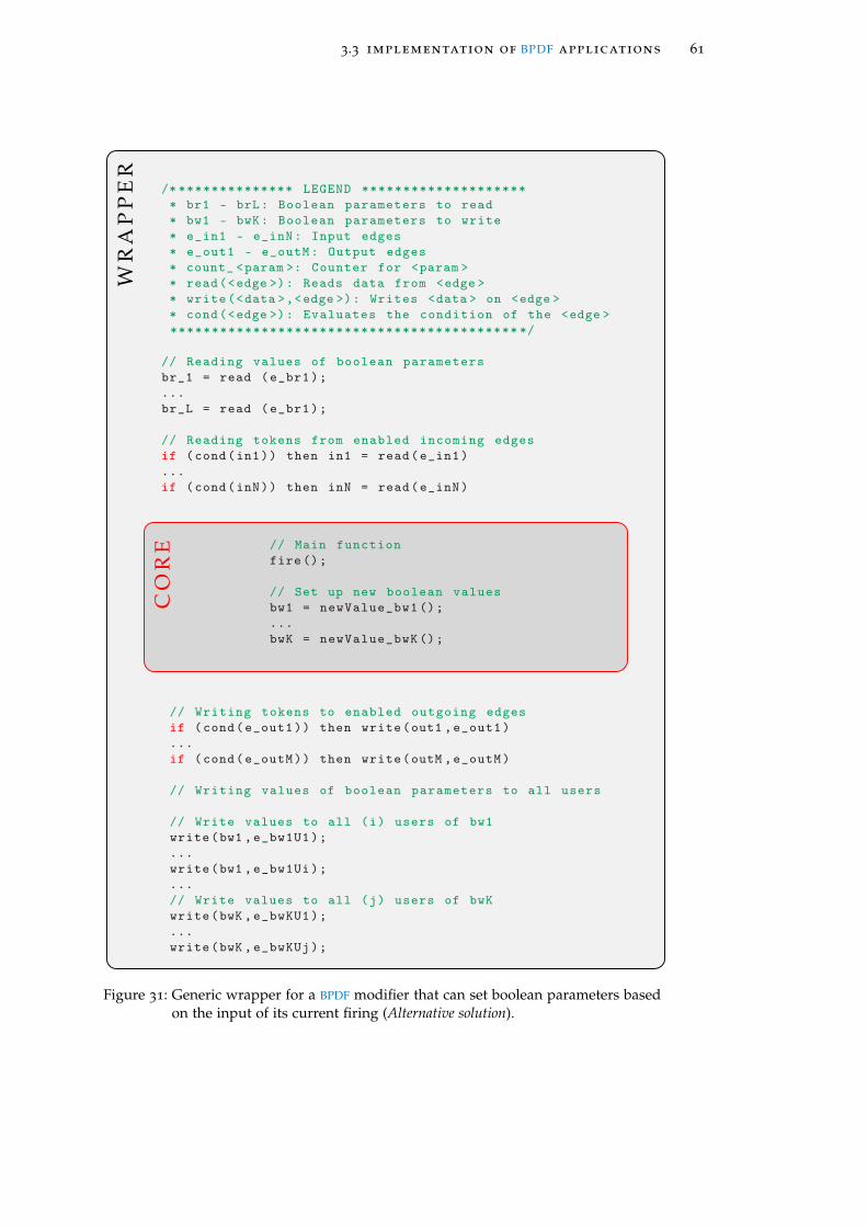
3.3 implementation of BPDF applications 61
CO
RE
WR
AP
PE
R
/* ************** LEGEND ********************
* br1 - brL: Boolean parameters to read
* bw1 - bwK: Boolean parameters to write
* e_in1 - e_inN: Input edges
* e_out1 - e_outM: Output edges
* count_ <param >: Counter for <param >
* read(<edge >): Reads data from <edge >
* write(<data >,<edge >): Writes <data > on <edge >
* cond(<edge >): Evaluates the condition of the <edge >
****************************************** */
// Reading values of boolean parameters
br_1 = read (e_br1);
...
br_L = read (e_br1);
// Reading tokens from enabled incoming edges
if (cond(in1)) then in1 = read(e_in1)
...
if (cond(inN)) then inN = read(e_inN)
// Main function
fire();
// Set up new boolean values
bw1 = newValue_bw1 ();
...
bwK = newValue_bwK ();
// Writing tokens to enabled outgoing edges
if (cond(e_out1)) then write(out1 ,e_out1)
...
if (cond(e_outM)) then write(outM ,e_outM)
// Writing values of boolean parameters to all users
// Write values to all (i) users of bw1
write(bw1 ,e_bw1U1);
...
write(bw1 ,e_bw1Ui);
...
// Write values to all (j) users of bwK
write(bwK ,e_bwKU1);
...
write(bwK ,e_bwKUj);
Figure 31: Generic wrapper for a BPDF modifier that can set boolean parameters basedon the input of its current firing (Alternative solution).

62 boolean parametric data flow
R X Mx r w yf(b1) g(b1,b2)
b1@π1 b2@π2#X #R
#M #R
#LM #LX
Figure 32: A BPDF graph expanded with its boolean propagation edges.
Consider the graph in Figure 32. Actor X is the modifier of b2 and a user of b1;it reads and writes tokens to and from conditional edges with a reading periodπr for b1, and a writing period πw for b2. The code in Listing 1 implementsone firing of X.
First, actor X must read the value of parameter b1 every πr = #X/freq(b1)
firings (the period safety ensures that this number is an integer). Countercount_b1 implements this periodic reading. If the input edge ĎRX is active,i. e., f(b1) = tt, then X consumes r tokens. Then, the actor executes its inter-nal function fire().
Actor X is also the modifier of b2, so it must send a new value to each user ofb2 every πw firings. Counter count_b2 keeps track of the writing period. Theedge between X and user M is denoted by e_b2M. Finally, if g(b1,b2) = tt, thenX produces w tokens on edge ĚXW.
Code wrappers implementing this periodic behaviour of reading and writ-ing boolean parameters can easily be produced automatically as shown in thegeneric wrapper in Figure 33. Their role is to synchronize the firings of modi-fiers and users for parameter communication. A user will be blocked waitingfor the modifier to produce the new boolean value that it needs. Thus, if a com-pletely disconnected actor can fire without constraint, it will eventually have towait in order to read (or write) a new boolean value.
Actually, this implementation can be described in a dataflow-like manner byadding edges between modifiers and users of the form
M U1
πw(b)1
πr(b)
where πr(b) denotes the reading period of b by U and a fractional rate, ab ,
means “produce/consume a tokens each b firings”. This representation is re-lated to an extension of SDF: the Fractional Rate Data Flow (FRDF) model [90].
3.3.3 Scheduling
In Section 3.2.3, we described a way to find sequential schedules for BPDF ap-plications. However, our objective is to use BPDF to implement streaming ap-plications on many-cores with highly parallel schedules. In such cases, it is

3.3 implementation of BPDF applications 63
CO
RE
WR
AP
PE
R/* ************** LEGEND ********************
* br1 - brL: Boolean parameters to read
* bw1 - bwK: Boolean parameters to write
* e_in1 - e_inN: Input edges
* e_out1 - e_outM: Output edges
* count_ <param >: Counter for <param >
* read(<edge >): Reads data from <edge >
* write(<data >,<edge >): Writes <data > on <edge >
* cond(<edge >): Evaluates the condition of the <edge >
****************************************** */
// Reading parameters values at the right periods
if (count_br1 == 0) then br_1 = read(e_br1);
...
if (count_brL == 0) then br_L = read(e_brL);
// Reading tokens from enabled incoming edges
if (cond(in1)) then in1 = read(e_in1)
...
if (cond(inN)) then inN = read(e_inN)
// Main function
fire();
// Set up new boolean values
bw1 = newValue_bw1 ();
...
bwK = newValue_bwK ();
// Writing tokens to enabled outgoing edges
if (cond(e_out1)) then write(out1 ,e_out1)
...
if (cond(e_outM)) then write(outM ,e_outM)
// Writing parameter values at the right periods
if (count_bw1 =0) then {
// Write values to all (i) users of bw1
write_p(bw1 ,e_bw1U1);
...
write_p(bw1 ,e_bw1Ui);
}
...
if (count_bwK =0) then {}
// Write values to all (j) users of bwK
write_p(bk ,e_bwKU1);
...
write_p(bk ,e_bwKUj);
}
/* Increment the counters modulo the
writing and reading periods */
count_bw1 = (count_bw1 +1) % pw_bw1;
...
count_bwK = (count_bwk +1) % pw_bwK;
count_br1 = (count_br1 +1) % (#X / freq(br1));
...
count_brL = (count_brL +1) % (#X / freq(brL));
Figure 33: Generic wrapper for a BPDF actor using periodic reading and writing ofparameters.
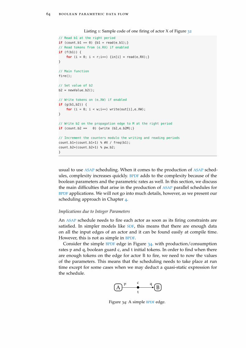
64 boolean parametric data flow
Listing 1: Sample code of one firing of actor X of Figure 32
// Read b1 at the right period
if (count_b1 == 0) {b1 = read(e_b1);}
// Read tokens from (e_RX) if enabled
if (f(b1)) {
for (i = 0; i < r;i++) {in[i] = read(e_RX);}
}
// Main function
fire();
// Set value of b2
b2 = newValue_b2();
// Write tokens on (e_XW) if enabled
if (g(b1,b2)) {
for (i = 0; i < w;i++) write(out[i],e_XW);
}
// Write b2 on the propagation edge to M at the right period
if (count_b2 == 0) {write (b2,e_b2M);}
// Increment the counters modulo the writing and reading periods
count_b1=(count_b1+1) % #X / freq(b1);
count_b2=(count_b2+1) % pw_b2;
}
usual to use ASAP scheduling. When it comes to the production of ASAP sched-ules, complexity increases quickly. BPDF adds to the complexity because of theboolean parameters and the parametric rates as well. In this section, we discussthe main difficulties that arise in the production of ASAP parallel schedules forBPDF applications. We will not go into much details, however, as we present ourscheduling approach in Chapter 4.
Implications due to Integer Parameters
An ASAP schedule needs to fire each actor as soon as its firing constraints aresatisfied. In simpler models like SDF, this means that there are enough dataon all the input edges of an actor and it can be found easily at compile time.However, this is not as simple in BPDF.
Consider the simple BPDF edge in Figure 34. with production/consumptionrates p and q, boolean guard c, and t initial tokens. In order to find when thereare enough tokens on the edge for actor B to fire, we need to now the valuesof the parameters. This means that the scheduling needs to take place at runtime except for some cases when we may deduct a quasi-static expression forthe schedule.
A Bp qc
t
Figure 34: A simple BPDF edge.

3.3 implementation of BPDF applications 65
However, the generation and analysis of a task graph of a given SDF graphcannot be afforded at run-time. For this reason, in Chapter 4, we introduce ascheduling framework that handles the generation of such a schedule in anefficient way.
Implications due to Boolean Parameters
Boolean parameters affect the scheduling procedure in two ways: first, they adddata dependencies due to the parameter communication edges, and secondlythey remove data dependencies at run-time based on the values of the booleanparameters.
In the case of the parameter communication edges, they can readily be dealtwith as edges of the graph that introduce additional data dependencies. How-ever, if the refined edges (Section 3.3.2) are used, the constraints need to berefined as well.
When an edge is deactivated, the scheduler should take it into account as itmay remove a data dependency, thereby allowing the consumer to fire earlier.Moreover, an actor may get completely disconnected and still fire. A firing withno input may be totally acceptable by the main functionality of the actor, andso it fires normally. However, for some actors it may not make sense to executewithout input. In these cases, the actor performs a dummy firing, i. e., a firingwithout calling its internal function, just to keep synchronized with the rest ofthe BPDF graph. These firings just adjust the internal counters of the actor.
3.3.4 BPDF Compositionality
So far, we have considered BPDF graphs that are flat, i. e., each actor is a primitivefunctional unit. However, one of the benefits of data flow models is modular-ity and the ability of developing complex applications from the compositionof multiple simple ones. Using composites has many benefits in applicationsdevelopment. It allows the separate development of parts of the applicationfrom different teams, the reusability of previously developed modules, and thescalability of the applications (by dealing with several smaller ones instead ofa single large application).
In such a setting, a graph may have actors that themselves are graphs. Suchactors are called composites. MoCs like PSDF [11], PiMM [37] and interfaced SDF [97]focus on such hierarchical compositions of applications.
In this section, we discuss the subtleties that arise when BPDF graphs are usedhierarchically. Each graph in a lower hierarchical level should have an interfacewith the higher hierarchical level, i. e., edges that connect the actors of the graphwith the ports of the composite actor. Such an actor is shown in Figure 35. Thecomposite has two inputs, connected to actors A and B with rates p and 2, andone output from actor D with rate of 1. We refer to these actors as interface actors
and the edges as interface edges. The rates of the interface of the composite arecomputed based on the rates of the interface actors and their solution in thecomposite. For an actor A with solution #A and port rate rA, we get the raterCA of the composite using:
rCA = #A ¨ rA (16)

66 boolean parametric data flow
A
B
C Dp p
b
¬b
b@1
p
2
1
r = [ABp Cp D]
M2 · #B
p · #A
#D
Figure 35: A BPDF composite.
In this way, one firing of the composite actor corresponds to the execution ofone iteration of the graph within the composite. In Figure 36a the compositeactor M is used in a BPDF graph. The equivalent flattened version of the graphis shown in Figure 36b.
An issue that arises in this scheme, is the usage of integer parameters. Ifthe interface actors have parametric solutions, then parent and child shouldshare these integer parameters. This limits the child to change these integervalues between iterations of the parent graph. However, if the interface of thechild has only fixed rates, or there are integer parameters that do not appear inthe solutions of the interface actors, then these integer parameters of the childcan change their values between iterations of the child graph, i. e., potentiallymultiple times within the iteration of the parent. As a consequence, such anhierarchical BPDF graph cannot be flattened into a BPDF graph.
Boolean parameters need to be considered too. Boolean parameters modifiedby an actor in the parent graph, can be safely used in the edges of the child astheir values will remain fixed during the iteration of the child. In this way, theywill have a frequency of 1 and all reading periods will equal the solution of theactor, satisfying the safety period. However, the definition of the region of theboolean parameters needs to be modified to include composite actors whosegraph include users of the boolean parameter.
It is best to prohibit modifiers of boolean parameters of the parent graph to beactors within a composite. Although the composite may act as a modifier for theparent, there may be cases that the modifier within the composite changes theboolean parameter multiple times during an execution of the composite whichraises the question of which value will be used in the parent. For this, booleanparameters should be limited on one hierarchical level at a time or ensure thata modifier in a lower level produces unique values. However, propagation of

3.4 model comparison 67
K
LM N
2p
p
q
q
(a) Composite actor M inside its top-levelBPDF graph.
A
B
C D
K
L Np p
2
pq q
b
¬b
b@1
M
(b) Equivalent BPDF graph without composites.
Figure 36: An hierarchical BPDF graph and its flattened equivalent.
boolean values across different levels of the hierarchy complicates the designand should be avoided.
3.4 model comparison
BPDF is a MoC that combines dynamic rates with dynamic topology. There areother models that have at least one of these two features as well. The main differ-ence between these MoCs is the trade-off between expressivity and analyzability.In this section we compare BPDF with models that have similar expressivity.
3.4.1 Boolean Data Flow
We single out the BDF MoC [21] from other MoCs because, despite its lack ofdynamic rates – all rates in BDF are fixed, it is the only model that focusesdirectly on dynamic topology. So, we will compare only this aspect with BPDF.
BDF uses two special actors that have as input a stream of boolean values. Thefirst one is the SWITCH actor which has one data input and two data outputsas well as a boolean input stream. Depending on the incoming boolean value,SWITCH activates the appropriate output. The second actor is called SELECTand has two data inputs and one data output and a boolean input stream. Theboolean value selects which input is active in this case.
BDF is shown to be Turing Complete in [21]. The problem arises in the bound-edness analysis of BDF. There can be cases where it is undecidable whether agraph is operating within bounded memory or not. Buck in his thesis [21] de-tails how a Universal Turing Machine can be built using BDF actors. Here, wegive an intuitive example that illustrates the problem. The graph in Figure 37

68 boolean parametric data flow
A
SWIT
CH
FT
FT
SEL
EC
T
B
C
D
b1 b2
1 1
1
1
1
1
1
1
1
1
1 1
Figure 37: A BDF graph that may operate in unbounded memory.
A
B
C
D1
1 1
1
1
1 1
1
b1
¬b1
b2
¬b2
b1@1b2@1
Figure 38: A BPDF graph similar to the BDF graph in Figure 37.
uses two different boolean streams to control the inputs and outputs of theSWITCH and SELECT actors respectively. Thus, assuming that the stream b1 isalways true, and the stream b2 is always false, it is easy to observe that therewill be an accumulation of tokens on the output of actor B. In order to guar-antee boundedness, one needs to show the equivalence of the two streams aproblem that Buck shows to be undecidable [21].
In some cases Buck provides a clustering technique to find a bounded sched-ule but the graph iteration is sacrificed. For example, the graph in Figure 39.The SWITCH actor provides tokens to actors B and C depending on the valuesof the boolean stream b. Actor B needs two tokens to fire. Assuming that b takesa tt value, allowing SWITCH to produce a token for actor B, and then takesff values producing tokens to actor C, there is no guarantee that the booleanstream will take a second tt value so that the token stored on the input edge ofB will be consumed. This means that there is no guarantee that the graph willever return to its initial state.
When it comes to BPDF, both these issues are dealt with thanks to the safety
period criterion and the fact that disconnected actors still fire without producingor consuming data. Safety period restricts BPDF expressivity so that it remainsanalyzable. Let us consider two examples of how BPDF would capture similarfunctionality as the two problematic BDF graphs.
In Figure 38 the two different boolean parameters, even if they are stuck at op-posite values, do not cause unboundedness. This is because actors B and C willproduce tokens regardless of the boolean value (i. e., even when disconnected),eventually enabling actor D to fire.
Finally, in 3Figure 40, the safety period criterion forces the boolean parameterto change value every two firings of actor A. This way if there is a tt value, it

3.4 model comparison 69
will last for two firings of A that will produce two tokens for actor B to fire.As a result, when the boolean parameter changes value, the input edge of B
returns back to its initial state preserving the iteration of the graph.
3.4.2 Schedulable Parametric Data Flow
Just like BDF, SPDF [43] focuses only on one aspect of dynamism, namely theparametric rates. The model does not support dynamic topology and we com-pare SPDF with BPDF only as far as the parametric rates are concerned.
SPDF uses the notion of regions, just like in the case of BPDF, to calculatechanging periods of integer parameters within an iteration. Changing integerparameters within an iteration adds a lot to the expressiveness of the modelbut also greatly increases its scheduling complexity. BPDF, on the other hand,allows integer parameters to change only between iterations. This way all ratesare known at the beginning of an iteration, reducing the scheduling complexity.
SPDF may potentially be combined with BPDF into a single MoC where both in-teger and boolean parameters change within an iteration. The resulting modelwill be very difficult to schedule apart from simple sequential and trivial paral-lel schedules.
3.4.3 Scenario-Aware Data Flow
Another model that stands out is SADF [116]. SADF uses special actors, called de-tectors, to change the rates of part of the graph. SADF allows dynamic topologyby allowing production and consumption rates of zero. Each different configu-ration is called a scenario.
In SADF, the set of possible scenarios that the graph may operate in needsto be defined. To capture a BPDF graph in SADF, all possible configurations ofthe graph need to be expressed and stored at compile time. In many cases thisis impractical, as the number of possible configurations of even a small BPDF
graph using a couple of parameters can be prohibitive.On the contrary, the enumeration of the scenarios in SADF has some advan-
tages. BPDF demands a graph to be consistent when all of its edges are active.In many cases, however, there are guards that use opposite boolean values andthe relevant edges are never active simultaneously. BPDF does not support analternative analysis where the graph is partially consistent, depending on the
A
SWIT
CH
FT
B
C
b
2 1
1
1
2
1
Figure 39: A BDF graph with problematic iteration.

70 boolean parametric data flow
A
B
C
1
2
1
1
b1
¬b1
b1@2
Figure 40: A BPDF graph similar to the BDF graph in Figure 39. The safety criterionguarantees that the graph will always return to its initial state.
values of the boolean parameters. The main reason behind this decision is tokeep the analysis of the graph independent of the values of the parameterswhich may lead to an explosion of different cases to verify.
SADF, on the other hand, renders such analysis feasible, by taking individualscenarios. Instead of analyzing the application for all possible values of theparameters, SADF focuses only in the much smaller subset of the values of thescenarios. In this sense, there may be SADF graphs that cannot be captured inBPDF, because they will be found to be inconsistent.
3.4.4 Other Models of Computation
There are other MoCs that combine dynamic rates and topology of lesser im-portance. As already mentioned in Chapter 2 models like CSDF and VRDF allowrates to take zero values effectively deactivating the port. However, in the caseof CSDF the sequence of change of the rates – and consecutively the activationand deactivation of the ports, is determined at compile time. VRDF allows onlyparameters that come in matching pairs, that is if there is a parametric produc-tion rate on a path, there must be the equivalent consumption rate on the samepath. Moreover, VRDF is limited to acyclic graphs only.
3.5 summary
In this chapter, we presented the BPDF MoC. The goal of this MoC is to providethe increased expressiveness needed for the efficient implementation of mod-ern streaming applications while still providing static analyses for consistency,boundedness and liveness.
BPDF accomplishes this by introducing integer and boolean parameters thatallow dynamic production and consumption rates on the edges of the graphsand dynamic topology changes. Integer parameters are changing once per it-eration, allowing a symbolic solution of the balance equations to be foundand most of the existing SDF techniques to be adapted to handle parameters.Boolean parameters are allowed to change periodically within an iteration ofthe graph by special actors called modifiers. BPDF introduces a supplementarycriterion, namely the period safety criterion, that ensures bounded and liveoperation of the graph regardless of the values of the boolean parameters.

3.5 summary 71
BPDF provides analyses for consistency, boundedness and liveness that areindependent of specific values of both the integer and the boolean parameters.For this reason, the model imposes additional constraints on the graph thatcould be otherwise lifted, like the demand of consistency on the graph whenall its edges are enabled.
We analyzed the subtleties that arise in the implementation of the model. Theimplementation choices, however, do not affect its static analyzes. Such choicesare, for example, the actions that compose the firing of a BPDF actor or the exactimplementation of the propagation of the boolean parameters.
Moreover, we saw that, due to the extra expressiveness, BPDF increases thecomplexity of the scheduling of the model. Dynamic rates change the numberof times that each actor should fire and dynamic topology may enable actorsearlier. Disconnected actors may fire, at least conceptually, without any inputsor outputs, to keep track with the advancement of the iteration. All these factorsneed to be taken into account by a scheduler to lessen overhead. We detail thescheduling of BPDF applications in Chapter 4.
Finally, we compared BPDF to other data flow MoCs of similar expressiveness.Compared to BDF that focuses on the boolean, and SPDF that focuses on the in-teger parameters, BPDF finds a trade-off between the two, where both types ofparameters are restricted on how often they can change values. This restrictionmakes BPDF analyzable and schedulable. A similar model, SADF, provides analternative solution useful in specific applications that cannot be captured byBPDF due to its restrictive consistency criteria. On the other hand, BPDF is prefer-able to SADF in applications where the large number of parameter combinationsprohibits the use of the latter. One can say that the two models complementeach other.


4S C H E D U L I N G F R A M E W O R K
It’s who I am and what I feelMy life is automaticUp in the air, it’s what I breatheand it is never static
— Amaranthe
The development of more expressive data flow models enables more complexapplications, such as video decoders, to be captured, but considerably increasesthe complexity of scheduling. As discussed in Chapter 3, parametric rates anddynamic topology both add challenges when it comes to parallel scheduling.Such dynamism prohibits the reuse of existing techniques; a DAG cannot be de-rived because of the parametric number of firings and the conditional connec-tions between them. In addition, manual production of such schedules wouldbe time consuming and error-prone.
This chapter describes a scheduling framework that allows the automatic pro-duction of parallel schedules for the deployment of BPDF applications on many-core platforms. The framework relies on the extraction of parametric schedulingconstraints from the application. To allow optimization and manual manipula-tion of the schedule, the framework also allows the user to add constraints thataffect the ordering and the parallel execution of the actors. These constraints areanalyzed to preserve the boundedness and liveness guarantees of the applica-tion. The resulting set of scheduling constraints is used to produce the parallelschedule.
The chapter starts with the overview of the underlying platform along withits mapping and scheduling assumptions in Section 4.1. Then, the proposedframework is presented in Section 4.2. Finally, the experimental evaluation ofthe framework is presented and discussed in Section 4.5.
4.1 underlying platform
BPDF is designed with streaming applications, like video decoders, in mind.Such applications are composed of computationally intensive functions andvery often have time restrictions. For example, a video needs to be decoded ata certain frame rate (i. e., 24 frames per second) to maintain an acceptable QoS.To meet such requirements, streaming applications are typically developed inspecialized hardware, sometimes with a software layer that allows the partialconfiguration of each hardware component.
We target the Sthorm many-core platform [87], formerly known as P2012.Developed by STMicroelectronics, Sthorm is a representative of a modernmany-core platform.
73

74 scheduling framework
STHORM C L U S T E R
H W P E # 1
HW
PU
HW
PU
HW
PU
· · ·
H W P E # 2
HW
PU
HW
PU
HW
PU
· · · · · · · · · · · · · · ·
H W P E # P
HW
PU
HW
PU
HW
PU
· · ·
C L U S T E R C T R L
D M A C H A N N E L # 0
D M A C H A N N E L # 1
C L U S T E R C T R L
I N T E R C O N N E C T
STXP70
E N C O R E C L U S T E R
ME
MO
RY
BA
NK
#1
ME
MO
RY
BA
NK
#2
ME
MO
RY
BA
NK
#3
· · ·
ME
MO
RY
BA
NK
#3
2
STXP70#1
STXP70#2 · · ·
STXP70#16
L O C A L I N T E R C O N N E C T ( S T R E A M F L O W )G
LO
BA
LIN
TE
RC
ON
NE
CT
INT
ER
FA
CE
EN
CO
RE
INT
ER
FA
CE
S T R E A M I N G I N T E R F A C E
C O M M C O M M C O M M
L O G A R I T H M I C I N T E R C O N N E C T
Figure 41: Architecture of a cluster of the Sthorm platform.
Sthorm is composed by up to 32 clusters interconnected by a global asyn-chronous NoC. Each cluster is composed by by a Cluster Controller, a multi-core computing engine called ENCore, and may optionally have a number ofspecialized Hardware Processing Elements (HWPEs).
The Cluster Controller manages the intra- and inter-cluster communication.It has a Global Interconnect Interface to access the Global NoC, a communicationinterface with the ENCore engine and a Streaming Interface with the HWPEs. Italso has a DMA module, allowing efficient communication of the ENCore engineand the HWPEs with each other and the global interconnect.
The ENCore engine can have up to 16 Software Processing Elements (SWPEs),which are general-purpose STxP70-V4 32-bit RISC processors. The STxP70-V4
processors use a centralized shared memory (UMA architecture) composed bymultiple banks that allow simultaneous access from all processors.
The HWPEs are further partitioned in Hardware Processing Units (HWPUs)that share the communication interface of the hosting HWPEs. The architectureof the Sthorm cluster is shown in Figure 41.
Sthorm includes a native programming model, Predicated Execution DataFlow (PEDF), that simplifies the parallel implementation of streaming applica-tions. PEDF uses filters to implement applications. A filter can be:
• A primitive filter is a filter that applies a well defined function to a set ofinput data in order to produce a set of output data. It is implemented asa hardware or software processing element and is the building block ofPEDF model.

4.1 underlying platform 75
• A module is a composite filter. A module can contain one or more prim-itive filters or modules. Modules allow the development of applicationshierarchically, facilitating the design.
• A controller which schedules the firing of the filters in a module and con-trols the configuration parameters for each filter. Each module contains itsown controller. If a module is fired, its controller is activated and executesits internal schedule, which fires the filters of the module.
4.1.1 Mapping
The scheduling framework focuses on the production of parallel schedulesgiven a static mapping and does not deal with mapping decisions.
In our implementation, a BPDF graph is implemented in PEDF using a singlemodule, hence the hierarchical composition of modules is not used. This is be-cause we assume BPDF graphs that do not use hierarchy. We discussed BPDF
compositionality in Section 3.3.4. Such an hierarchical model can take advan-tage of PEDF modules where each module is a BPDF graph.
The module contains one PEDF primitive filter for each BPDF actor, whichcorresponds to a separate (hardware or software) processing element. Integerparameter and boolean parameters communication takes place through the con-troller of the module by changing corresponding configuration parameters ofeach filter. The controller also controls the execution of the application.
This is a simple yet realistic mapping scheme. Although, in this mappingscheme, each actor is mapped on a separate processing element, the frame-work can handle any other kind of static assignment, where actors may shareresources as discussed in Section 4.4.2.
4.1.2 Scheduling
The goal of our scheduling framework is the generation of the controller thatcontrols the schedule of each BPDF actor. The PEDF model uses slotted scheduling
(Section 2.4.5) to schedule the firing of the filters. At the beginning of a slot,the controller selects several filters to be fired and their execution takes placeconcurrently. When these executions are completed, the next slot may start. Thecontroller may compute the composition of the next slot while the filters of thecurrent slot execute, therefore the hardware pipeline is not slowed down.
We produce slotted schedules that can be directly implemented using thismodel. Such a framework can also be used by other state-of-the-art many-coreplatforms. For instance, modern GPUs support a similar execution model. Inmainstream GPU programming models, such as CUDA [28] and OpenCL [112],the host processor, equivalent to the controller of Sthorm, creates a task group,loads it on the GPU, and gets the results when all tasks have finished theirexecution. In parallel with the execution of the task group, the host processormay determine tasks to be executed next.
Although it relies on the Sthorm platform, our scheduling framework can beeasily adapted to produce non-slotted schedules, as discussed in Section 4.4.1.

76 scheduling framework
B P D F
A P P L I C AT I O N
U S E R - D E F I N E D
C O N S T R A I N T S
O R D E R I N G
C O N S T R A I N T S
R E S O U R C E
C O N S T R A I N T S
S I M P L I F I C AT I O N
& L I V E N E S S
E VA L U AT E
O R D E R I N GF I LT E R I N G
A S A P
S C H E D U L E
Scheduler
Figure 42: Our Scheduling Framework.
4.2 scheduling framework
The goal of our framework is to produce ASAP parallel schedules. ASAP sche-duling is chosen because it is considered to be the best strategy when timinginformation about the execution of the actors is unknown [111]. Unknown tim-ing is typical for BPDF applications where the execution time of the actors mayvary a lot, based on the values of the integer and boolean parameters.
Our framework also aims to be flexible and expressive in order to supporta multitude of platforms and different optimization criteria. Our frameworkuses a fixed scheduling algorithm (here ASAP) and allows the schedule to bemanipulated by adding new scheduling constraints that affect the ordering andthe parallel execution of the actors.
An overview of the framework is shown in Figure 42. The framework receivesthe BPDF application along with an optional set of user-defined constraints.From these, a set of ordering constraints and a set of resource constraints areproduced. The resulting ordering constraints (i. e., those extracted from the BPDF
graph and those added by the user) are checked for liveness and, if possible,simplified. Then, the ASAP scheduler produces the ASAP parallel schedule meet-ing the constraints one slot at a time. Each slot is produced in two stages; firstthe ordering constraints are evaluated to produce a set of fireable actors, then,the set of fireable actors is filtered, according to the resource constraints, to pro-duce a subset of fireable actors that will eventually fire in the slot. The schedulercontinues until the iteration is completed.
Scheduling constraints derive both from the application and express the de-pendencies of the dataflow graph, or from the user expressing platform speci-ficities (e. g., resource limitations), or optimizing some criteria (e. g., power con-sumption, buffer sizes). They can be of two distinct types: Ordering constraints
that restrict individual actor firings, and resource constraints that control parallelexecution (e. g., limiting the level of parallelism). Application constraints canonly be ordering constraints. User constraints can be both resource and order-ing constraints. They are defined by the programmer for a specific application
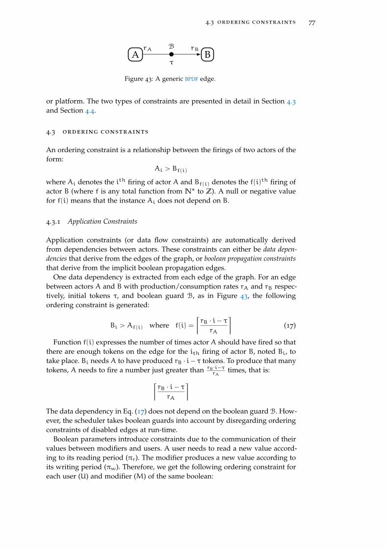
4.3 ordering constraints 77
A BrA rBB
τ
Figure 43: A generic BPDF edge.
or platform. The two types of constraints are presented in detail in Section 4.3and Section 4.4.
4.3 ordering constraints
An ordering constraint is a relationship between the firings of two actors of theform:
Ai ą Bf(i)
where Ai denotes the ith firing of actor A and Bf(i) denotes the f(i)th firing ofactor B (where f is any total function from N
˚ to Z). A null or negative valuefor f(i) means that the instance Ai does not depend on B.
4.3.1 Application Constraints
Application constraints (or data flow constraints) are automatically derivedfrom dependencies between actors. These constraints can either be data depen-
dencies that derive from the edges of the graph, or boolean propagation constraints
that derive from the implicit boolean propagation edges.One data dependency is extracted from each edge of the graph. For an edge
between actors A and B with production/consumption rates rA and rB respec-tively, initial tokens τ, and boolean guard B, as in Figure 43, the followingordering constraint is generated:
Bi ą Af(i) where f(i) =
RrB ¨ i´ τ
rA
V(17)
Function f(i) expresses the number of times actor A should have fired so thatthere are enough tokens on the edge for the ith firing of actor B, noted Bi, totake place. Bi needs A to have produced rB ¨ i´ τ tokens. To produce that manytokens, A needs to fire a number just greater than rB¨i´τ
rAtimes, that is:
RrB ¨ i´ τ
rA
V
The data dependency in Eq. (17) does not depend on the boolean guard B. How-ever, the scheduler takes boolean guards into account by disregarding orderingconstraints of disabled edges at run-time.
Boolean parameters introduce constraints due to the communication of theirvalues between modifiers and users. A user needs to read a new value accord-ing to its reading period (πr). The modifier produces a new value according toits writing period (πw). Therefore, we get the following ordering constraint foreach user (U) and modifier (M) of the same boolean:

78 scheduling framework
Ui ąMf(i) where f(i) = πw ¨
Zi´ 1
πr
^+ 1 (18)
Function f(i) expresses the number of times that the modifier should fireto produce the value of the boolean parameter used by the user on its ith
firing (Ui). Actor U reads a new boolean value every πr firings, so Ui will needthe kth value of the boolean parameter to fire, where k is
k =X(i´ 1)/πr
\+ 1 (19)
The modifier produces a value every πw firings, hence the kth boolean value isproduced on its mth firing, where m is.
m = πw ¨ (k´ 1) + 1 (20)
Therefore, we replace k in Eq. (20) by the required value of Eq. (19), yielding:
πw ¨
(Zi´ 1
πr
^+ 1´ 1
)
+ 1 = πw ¨
Zi´ 1
πr
^+ 1
which indicates the number of times the modifier needs to have fired to producethe needed value. The constraint restricts the user to wait for the productionof a boolean value but does not restrict the modifier. Indeed, the modifier mayproduce a new boolean value (or all the boolean values) before the user hasfinished using the previous one. The user will use the new values later, basedon its reading period, when they are needed.
It is worth to note here that this is the weakest constraint that the booleanpropagation imposes on the user of a parameter. As discussed in Section 3.3.2,the actual implementation may impose stronger constraints. If the propagationof the boolean values is implemented with simple data flow edges, as suggestedin Section 3.2.3, then the boolean propagation constraints can be derived as datadependencies from the additional edges.
Finally, as we consider each actor executing on a single processing element(hardware or software), we have the implicit self-constraint for each actor X:
Xi ą Xi´1 (21)
which expresses the fact that there can not be multiple instances of an actor ex-ecuting in parallel and that the firings of the same actor take place in sequence.
The self dependency expressed in Eq. (21) is derived from the given map-ping decision that requires each actor on a different processing element. InSection 4.4.2, we demonstrate how alternative static mapping schemes, usingdata parallelism, can be expressed.
4.3.2 User Ordering Constraints
Additional user ordering constraints can be used to optimize various criteria(e. g., power consumption, buffer size). Here we give a few examples of userconstraints that achieve various improvements.
Consider again the generic BPDF graph of Figure 43. For simplicity and with-out loss of generality, we consider the rates rA and rB to be co-primes. Hence,

4.3 ordering constraints 79
the repetition vector of the graph is [ArB BrA ] and A will fire rB times withoutany constraints. Since A fires rB times consecutively, if B does not consumeenough tokens, there will be an accumulation of tokens on the FIFO buffer fromA to B.
If the programmer wants to restrict this FIFO buffer to be of a certain size,say k tokens, the execution of A needs to be regulated so that it fires only whenthere is enough space left on the edge buffer. Adding the following backwardsconstraint from B to A:
Ai ą Bf(i) where f(i) =
RrA ¨ i´ k+ τ
rB
V(22)
enforces the buffer size to be at most k.Typically, in data flow graphs a buffer constraint of k tokens is modeled by
adding a backward edge from B to A with k´ t initial tokens, so that the totalnumber of tokens on the AB cycle will be k. Extracting the data dependencyfrom such an edge, gives the constraint expressed in Eq. (22).
Additional user-defined constraints may introduce a deadlock if they arenot compatible with the data dependency constraints extracted from the BPDF
application. For instance, in the previous example, it should be checked that kis large enough so that A can trigger all rA firings of B. This verification step isdone using a deadlock detection algorithm presented in Section 4.3.3.
4.3.3 Liveness Analysis
Inconsiderate user-defined constraints must be checked statically for liveness.A set of ordering constraints may introduce deadlock when they imply (bytransitivity) a constraint of the form:
(Ai ą Aj)^ (i ď j) (23)
which requires that the ith firing of an actor A must take place after the jthfiring where j is the same or a future firing (j ě i). All cyclic constraints froman actor to itself must be checked. The complexity of liveness analysis is linearto the number of cyclic constraints. To ensure liveness, it must be shown thateach cycle of the form:
Ai ą Bf1(i) ą . . . ą Cfn(i) ą Afn+1(i)
that is to sayAi ą Af1(...(fn(fn+1(i)))...)
satisfiesi ą f1(. . . (fn(fn+1(i))) . . .) (24)
We consider all ordering constraints to detect such cycles. Typically, the ex-pression f1(. . . (fn(fn+1(i))) . . .) contains parameters and ceiling functions. Ingeneral, only an upper bound can be computed. Parameters are replaced bytheir maximum or minimum values and ceilings
Pab
Tby a
b + 1 or ab ´ 1 depend-
ing on their sign and position. The expression f1(. . . (fn(fn+1(i))) . . .) is thensimplified to get an upper bound. If the condition in Eq. (24) is true for all cycles,

80 scheduling framework
then the liveness of the schedule is guaranteed. Otherwise, since we have com-puted an over-approximation, we cannot guarantee that the set of constraints isnot live but we still reject the graph.
Consider, for instance, the simple BPDF graph in Figure 44.
A Bp q
Figure 44: A simple BPDF graph.
The data dependency we obtain from the edge is:
Bi ą Af(i) with f(i) =
Rq ¨ i
p
V
When the user wants to limit the edge buffer to k tokens, she introduces thefollowing constraint:
Ai ą Bg(i) with g(i) =
Rp ¨ i´ k
q
V
Together they form a cyclic constraint:
Ai ą Af(g(i))
In practice, such a limit (k) as well as the maximum values of parameters (pmax,qmax) are actual integers. Here, we illustrate the verification process using sym-bolic values. Based on Eq. (24), to ensure liveness we must verify that:
i ą f(g(i)) ô i ą
Rq¨rp¨i´k
q sp
V
ð i ąq¨(p¨i´k
q +1)
p + 1
ô i ą i+ q´kp + 1
ô k ą p+ q
ð k ą pmax + qmax
So, if the limit placed on the buffer size k is greater than pmax + qmax, a liveschedule is ensured. This is only a sufficient condition, because of the approxi-mation incurred by removing the ceiling functions.
In general, if there exists a cycle that does not satisfy Eq. (24), then the in-volved user constraints are rejected. Actually, this cycle condition can be re-laxed by taking boolean guards into account. The scheduler takes into accountthe boolean values, hence if two constraints of a cycle depend on on contradic-tory boolean guards, then the cycle is live as it cannot be formed.
Consider the simple BPDF graph in Figure 45. The graph contains a false cycleC = tA,Bu. As discussed already in Section 3.2.3, such cycles do not introducea deadlock because they are never formed at run-time. However, the cycle hastwo ordering constraints:
Ai ą Bi and Bi ą Ai

4.3 ordering constraints 81
that form the cyclic dependency:
Ai ą Bi ą Ai
which obviously does not satisfy the criterion in Eq. (24).Checking for false cycles in the cycles formed by scheduling constraints is not
the same as in the liveness analysis because instead of actors we have instancesof actors. Hence, one should take into account the reading periods of the actors,to make sure that the involved instances use the same boolean value of thecontradicting parameter.
4.3.4 Scheduler
For a set of constraints, the goal is to find the actors that will fire in each slot or,equivalently, to find the slot at which each firing takes place. The assignmentof a slot to each firing must be a valid solution to the set of constraints.
A function that assigns the firings of an actor to slots is called a firing function.For the firings of actor A, Ai, we get the firing function Φ(Ai) : F(Ai) Ñ L,where F(Ai) is the set of firings of actor A and L is the set of the schedule slots.
As we want to get the ASAP schedule meeting the constraints, each firing Ai
should be scheduled at the earliest slot possible, that is the first slot after all theactor instances Ai depends on, have fired. A firing Ai, with a set of constraintsC(Ai), depends on a set of firings F(Ai) that derive from C(Ai). If C(Ai) is:
C(Ai) = Ai ą B1f1(i), Ai ą B2f2(i), . . . ,Ai ą Bnfn(i)
(
then we get the set of firings:
F(Ai) = B1f1(i), B2f2(i), . . . ,Bnfn(i)
(
Therefore, the firing function for Ai is:
Φ(Ai) =
$&
%
maxkP[1,n]
(
Φ(
Bkfk(i)
))
+ 1 if i ą 0
0 if i ď 0
(25)
Ordering constraints may be deactivated depending on boolean conditions.The firing function takes into account these conditions as well. So, if F(Ai)
depends on n boolean conditions (L1,L2, . . . ,Ln) the firing function given inEq. (25) becomes:
Φ(Ai) =
$&
%
maxkP[1,n]
(
Lk ? Φ(
Bkfk(i)
)
: 0)
+ 1 if i ą 0
0 if i ď 0
(26)
M A B
b
¬bb@1
Figure 45: A BPDF graph with a false cycle.

82 scheduling framework
where Lk ? Φ(
Bkfk(i)
)
: 0 means that if condition Lk is true, then the firingfunction of Bkfk(i) is considered normally and if it is false 0 is used instead.
For readability, we suppress the 0 part and write: Lk ? Φ(
Bkfk(i)
)
instead.Moreover, we will define firing functions using only the part where i ą 0.
As all actors have the implicit self-constraint of Eq. (21) in their set of con-straints, their previous firing is in the set of firings (Ai´1 P F(Ai)). For thisreason, all firing functions are strictly monotonic, that is:
Φ(Ai) ą Φ(Ai´1) (27)
For example, consider an actor A with ordering constraints
Ai ą Bf(i) and Ai ą Cg(i)
with constraint Ai ą Bf(i) depending on boolean parameter b, and the self-constraint Ai ą Ai´1, has
F(Ai) = tBf(i),Cg(i),Ai´1u
and will have the firing function:
Φ(Ai) = max(
Φ(
b ? Bf(i)
)
, Φ(
Cg(i)
)
, Φ (Ai´1))
+ 1 if i ą 0
A scheduler is used to execute the graph (Alg. 2). It takes as input the repe-tition vector (R) and the set of actors (A) along with their firing functions (Φ).Moreover, the scheduler gets the reading and writing periods of the actors (Π).
The scheduler uses a status vector (Vs) that keeps track of the number oftimes an actor has fired, a next slot vector (Vn) that indicates the slot numberthat the next firing of an actor will take place, and a fire vector (Vf) that indicatesthe actors that fire in the current slot. The current slot number is kept in thevariable ℓ.
The scheduler is an infinite loop that schedules one iteration at a time. At thebeginning of an iteration, the Vs vector and the current slot number ℓ are initial-ized respectively to ~0 and 0. Then, the scheduler reads the current values of theinteger parameters (I) and evaluates the repetition vector, the firing functions,and the writing and reading periods.
The core of the scheduler is a for-loop over the set of actors, which selectsthe eligible actors for the current slot. Before entering the loop, the current slotnumber is increased by 1 and Vf is initialized to ~0. The for-loop first updatesthe next slot (Vn) value of each actor using its firing function, then checkswhether the actor is eligible to fire in the current slot. If the actor A is eligibleand still has firings left for the current iteration (i. e., Vs[A] ă R[A]), it is markedto be fired in the firing vector (Vf[A] = 1) and its status Vs[A] value is increasedby 1.
Firing functions depend on their previous values as well as on values of otherfiring functions. For this reason, the computed values of each firing function arekept in memory to avoid re-computation.
If a firing generates a new boolean value, the values of the boolean parame-ters (B) are updated. These are kept in lists (one list for each parameter) whichare initially empty. The boolean values are needed for the evaluation of the

4.3 ordering constraints 83
Algorithm 2 ASAP Scheduler that uses firing functionsprocedure scheduler(R,A, Φ, Π)
while true do
Vs = ~0
ℓ = 0
I = get int values()
R = evaluate(R, I)Φ = evaluate(Φ, I)Π = evaluate(Π, I)while Vs ‰ R do
ℓ = ℓ+ 1
Vf = ~0
for @X P A do
Vn[X] = Φ(X, Vs[X] + 1, B)
if Vn[X] == ℓ^ Vs[X] ă R[X] then
Vf[X] = 1
Vs[X] = Vs[X] + 1
if newbool() then
B = get bool values()
end if
end if
end for
fire(Vf)
end while
end while
end procedure
firing functions. The reading periods are used to get the correct value of theboolean parameter from the corresponding list. For a firing Ai using boolean b,with writing period πA
r (b), the kth value of boolean parameter is used, where:
k =
Ri
πAr (b)
V
Once the for-loop is finished, the firing vector is issued to fire. The for-loop isnested within a while-loop over the iteration of the graph. The outer loop endsonce the status vector equals the repetition vector of the graph. Liveness anal-ysis guarantees that at least one firing will take place every time the for-loop
executes and that the while-loop will end.
4.3.5 Constraint Simplification
Once the constraints are verified to preserve liveness, they are simplified. Thesimplification step consists of two parts:
• Constraint trimming, where redundant constraints are removed.• Constraint resolution, where constraints are resolved into slot sequences
at compile time if possible.

84 scheduling framework
Constraint Trimming
Constraint trimming checks the firing functions (Φ) in the max function ofEq. (25) and removes the firing functions that can be compared at compile time.For each pair of firings‚ When the firing functions to be compared are of the same actor, because
of the monotonicity of the firing function (Eq. (27)), we only need to comparetheir indexes.
For an actor A with
Φ(Ai) = max(
Φ(Bf1(i)),Φ(Bf2(i)), . . .)
+ 1
if f1(i) ą f2(i), then Φ(Bf2(i)) is suppressed.‚ When the firing functions are of different actors, then comparison may be
possible by transitivity through a third firing function.For an actor A with
Φ(Ai) = max(
Φ(Bf(i)),Φ(Cg(i), . . .))
+ 1
and a firing function of C depending on B:
Φ(Ci) = Φ(Bk(i)) + 1
ñΦ(Cg(i)) = Φ(Bk(g(i))) + 1
if k(g(i)) ě f(i) then Φ(Bf(i)) is suppressed from Φ(Ai).When constraint trimming takes place, the boolean parameters should be
taken into account. When a constraint Φ(Bj) suppresses constraint Φ(Ck) in fir-ing function Φ(Ai), it should be checked whether the constraint Φ(Bj) dependson a boolean parameter. Trimming can not take place when constraint Φ(Bj)
can be suppressed due to boolean parameters because then constraint Φ(Ck) isno longer redundant.
Constraint Resolution
In some cases, we can solve the firing functions of each or some of the actors, atcompile time. Solving a firing function means to define it in terms of a simplenon recursive function of its index and other firing functions that are alreadysolved. Such definitions derive inductively from Eq. (25) when the max functioncan be evaluated at compile time. The evaluation of the max function is possiblein many cases. Here, we provide a non-exhaustive list of the more prominentcases:‚ For source actors, the max function of the firing function contains only the
previous firing of the actor:
Φ(Ai) = Φ(Ai´1) + 1
It is easy to show that the firing function of such actors is the identity function:
Φ(Ai) = i (28)
‚ When the actor depends on a single firing that has already been defined asa constant:
Φ(Ai) = max (c,Φ(Ai´1)) + 1

4.3 ordering constraints 85
then the firing function can be simplified into:
Φ(Ai) = i+ c (29)
‚ Another interesting case is the simple data dependency between a consumerand a producer when the firing function of the producer is already solved.Consider an edge as the one in Figure 44 (p. 80). The data dependency betweenthe two actors is Bi ą Af(i), where f(i) =
Pqip
T. Based on Eq. (25), the firing
function of B is:
Φ(Bi) = max(
Φ(
Arqip s
)
,Φ(Bi´1))
+ 1
We show that the firing function in this case is:
Φ(Bi) =
$’’&
’’%
Φ(
Arqip s
)
+ 1 if q ą p
Φ(A1) + i if q ď p
(30)
Proof. By induction. For the case where q ą p, the expression holds for i = 1:
Φ(B1) = max(
Φ(
Arqp s
)
,Φ(B0))
+ 1 = Φ(
Arqp s
)
+ 1
Assuming that
Φ(Bn) = Φ(
Arqnp s
)
+ 1
we show that
Φ(Bn+1) = Φ
(
AQq(n+1)
p
U)
+ 1
Indeed,
Φ(Bn+1) = max(
Φ
(
AQq(n+1)
p
U)
,Φ (Bn)
)
+ 1
= max(
Φ
(
AQq(n+1)
p
U)
,Φ(
Arqnp +1s
)
)
+ 1
Furthermore:
q ě p ñ
Rqn+ q
p
Vě
Rqn+ p
p
V=
Rqn
p
V+ 1
and since all firing functions are strictly monotonic (Eq. (27)), this yields:
Φ
(
AQq(n+1)
p
U)
ě Φ(
Arqnp s+1
)
Hence,
Φ(Bn+1) = Φ
(
AQq(n+1)
p
U)
+ 1
The case q ď p is proved in a similar way.

86 scheduling framework
With the above simplification cases, we end up with a variety of differentdefinitions of the firing functions.
In the particular case of SDF, they can be defined using only indexes. In thiscase, one can compute the schedule slots for each actor A by evaluating thefiring function for i P [1..#A]. In this way, static slot sequences can be producedfor each actor.
Firing function definitions may also include integer parameters as is the caseof Eq. (30). In this case, we may be able to produce parameterized slot sequencesfor each actor and produce a single schedule stream using the procedure inAppendix A.1.
To illustrate the various cases, we consider again the simple graph in Fig-ure 44 (p. 80). Actor A is a source actor and its firing function is (Eq. (28)):
Φ(Ai) = i with i P [1,q]
which corresponds to the slot sequence Fq, meaning that A fires for q consec-utive slots. For actor B we distinguish the following cases:case q ď p : Using Eq. (30) we get
Φ(Bi) = i + 1 with i P [1 , p]
Hence, the sequence of slots of actor B is EFp meaning that B is idleduring the first slot and then fires at each slot. The execution will proceedas follows: A fires in the first slot and for each subsequent slot, A will firein parallel with B until it has fired a total of #A = q times. This totalsto q´ 1 firings of B so there remains to fire B another p´ (q´ 1) times.Hence, the two slot sequences can be combined in a slotted schedule (seeAppendix A.1 for an algorithm that merges such expressions):
A; (A}B)q´1;Bp´q+1
case q ą p : Two sub-cases must be considered:sub-case q = k ¨ p : If q is a multiple of p, using Eq. (30) with q ą p:
Φ(Bi) =
Rqi
p
V+ 1 =
Rkpi
p
V+ 1 = ki + 1 with i P [1 , p]
Each firing of B occurs after k firings of A and the corresponding slotsequence is E(Ek´1F)p. The two slot sequences can be combined ina slotted schedule:
A; (Ak´1; (B}A))p´1;Ak´1;B
sub-case q = k ¨ p + r with 0 ă r ă p : In this case, Eq. (30) yields:
Φ(Bi) =
Rqi
p
V+ 1 with i P [1 , p]
The slot sequence of B cannot be expressed as before because theceiling in the firing function cannot be resolved and needs to becomputed at run-time.

4.3 ordering constraints 87
A B C2p 3 2
3pb
b@2
Figure 46: A BPDF graph whose constraints can be solved symbolically.
In the last case, the firing functions could not be expressed as a slotted sched-ule. Still avoiding the evaluation of the set of constraints at run-time and using afixed firing function instead is a large improvement. One can observe that evenwhen the relation between the parameters is unknown, with a single conditionat runtime we can effectively use simplified results. This makes the schedulefaster, as we reduce the calculations done at run-time, but may increase theschedule code size. So, we have a trade-off between performance and memory.
The above cases are just a small sample of the possible firing functions thatcan be solved at compile time. Other cases and simplifications are presentedin [30].
Simplification Example
Consider the graph in Figure 46, whose iteration is [A B2p C3p] and whosedataflow constraints are:
Bi ą Ar i2p s, i P [1, #B]
Cj ą Br 2j3 s, Cj ą Ar j
3p s, j P [1, #C]
plus the implicit Xi ą Xi´1 for all actors. Moreover, actor C, as a user of theboolean parameter b, is constrained by (from Eq. (18)):
Cj ą B2t j´1
3 u+1ñ Cj ą B
2r j3 s´1
because of the floor property:
Y nm
]=
Rn´m+ 1
m
V=
Rn+ 1
m
V´ 1
This transformation is useful because all the constraints involve only ceilingfunctions.
We notice that although actor C has two constraints from actor B that seemredundant, they are not trimmed because, as explained in the previous section,the prevailing constraint is depending on the boolean parameter b.
Actor A is a source actor and from Eq. (28), we have:
Φ(Ai) = i with i = 1 (#A = 1)
So, we schedule A1 in the first slot (Φ(A1) = 1) and the slot sequence of actorA is F.
The constraint for actor B becomes Bi ą A1, i P [1, #B], hence:
Φ(Bi) = max (Φ(A1),Φ(Bi´1)) + 1 = max (1,Φ(Bi´1)) + 1

88 scheduling framework
Actor B is depending on a constant firing so, from Eq. (29), we have:
Φ(Bi) = i+ 1, with i P [1, 2p]
and the slot sequence of B is EF2p. Finally, the three constraints on actor C
yield the following firing function:
Φ(Ci) = max(
Φ(A1),b?Φ(
Br 2i3 s
)
,Φ(
B2r i3 s´1
)
,Φ(Ci´1))
+ 1
= max
(
1,b?(R
2i
3
V+ 1
)
, 2Ri
3
V,Φ(Ci´1)
)
+ 1, i P [1 . . . 3p]
‚ When b is tt,P2i3
T+ 1 is not suppressed, and since:
@i,R2i
3
V+ 1 ą 2
Ri
3
Vą 1
we get:
Φ(Ci) = max
(R2i
3
V+ 1,Φ(Ci´1)
)
+ 1, i P [1, 3p]
where we have the case of a firing function depending on single data depen-dency. Hence, from Eq. (30) we get:
Φ(Ci) =
R2i+ 3
3
V+ i = i+ 2, i P [1, 3p]
‚ When b is ff, the firing function becomes:
Φ(Ci) = max
(
2
Ri
3
V,Φ(Ci´1)
)
+ 1, i P [1, 3p]
Again, we have the form of a single data dependency and, from Eq. (30), weget:
Φ(Ci) = 2
R1
3
V+ i = i+ 2, i P [1, 3p]
We notice that in both cases, the solution for actor C is:
Φ(Ci) = i+ 2, i P [1, 3p]
As a result, the value of the boolean parameter does not influence the solution.The slot sequence of actor C is E2F3p. Having found the slot sequences of allactors:
A :F
B :EF2p
C :E2F
3p
we can merge them into a single schedule stream using the procedure presentedin Appendix A.1:
A;B; (B}C)2p´1;Cp+1
4.4 resource constraints 89
4.4 resource constraints
Resource constraints are used to regulate the parallel execution of actors. Suchconstraints can be used to limit the degree of parallelism or to enforce mutualexclusion between (groups of) actors. They can be seen as filter functions ap-plied to the set of fireable actors S and returning a subset T of S. Any suchfunction f must satisfy the two following conditions:
@S, f(S) = T ñ T Ď S (31)
@S, f(S) = T ñ T ‰ H (32)
The condition in Eq. (31) ensures that the function is safe (only firable actors canbe selected), while the condition in Eq. (32) ensures that it preserves liveness(at least one actor is selected to be fired).
Many languages can be used to express such constraints. Since they are func-tions over finite domains, one may even consider expressing them exhaustivelyas tables. Here, we use rewrite rules on sets inspired from the Gamma formal-ism [3]. The general form of a resource constraint is:
replace SA by SB if condition (33)
where SA and SB are nonempty sets of enabled actors such that SB Ď SA. Itcan be read as “replace SA by SB if condition is true”. When the condition isalways true it can be omitted. For example, the rule
replace A, B by A (34)
can be read as “if the actors A and B are fireable, then replace them by A
(i. e., remove B)”. It prevents actors A and B from being fired in the same slotand gives priority to A.
Rewrite rules can use pattern variables to match arbitrary actors. For instance,the rule
replace w, x,y, z by w, x,y (35)
can be read as “select four arbitrary fireable actors and suppress one of them”.It limits the level of parallelism to 3 actors. Indeed, rewriting rules apply untilno match can be found. Therefore, Rule (35) above applies as long as there aremore than three firable actors.
Rules can also depend on a condition. For instance, assuming that the twopredicates short and long denote whether an actor takes a short or long time toexecute, the rule
replace x, y by x if short(x)^ long(y) (36)
prevents short and long actors from being fired within the same slot (priorityis given to short ones). This rule may improve the overall computation time.Indeed, if S is a “short” actor while L1 and L2 are two “long” actors such thatS and L1 are fireable at the same slot and firing S enables L2, then it is better tofire first S alone and then L1 and L2 in parallel. The effect of the constraint inthis case is shown in Figure 47, where Figure 47a is the slotted schedule beforeapplying Rule (36) and Figure 47b after.

90 scheduling framework
1 2 3 4 5 6 7
L1 L1
L2 L2
S S
(a) Initial schedule.
1 2 3 4 5 6 7
L1 L1
L2 L2
S S
(b) Schedule after rule is applied.
Figure 47: Possible effect of the resource constraint. (Rule (36))
In a similar manner we can limit the power consumption during a slot. As-suming two predicates that classify actors into high (H) or low (L) power con-sumers, we can limit power consumption by firing at most one H actor eitheralone or along with at most one L actor. The following set of rules implementssuch a limitation:
replace x, y by x if H(x)^H(y)
replace x, y, z by x, y if H(x)^ L(y)^ L(z)(37)
Several rules can also be combined in sequence or in parallel. The semanticsof parallel composition enforces that rules applied in parallel act on disjointsets of actors. For example, the sequential combination of Rule (36) followedby Rule (35) limits the possible parallel firings to one actor, two short actors,or two long actors. The application of Rule (35) followed by Rule (36) imposethe same limitation but the results will differ as Rule (36) followed by Rule (35)gives priority to short actors.
It is very easy to check that such rules preserve boundedness and liveness. Itis sufficient to check that each rule obeys the conditions in Eq. (31) and Eq. (32).
Resource constraints have to be applied dynamically. They can either be re-solved by an iterative application of the rules until no rule can be applied,or they can be statically compiled, considering all sets of fireable actors, intoconstant time selection operations. The two approaches trade-off run-time per-formance with memory usage.
4.4.1 Alternative Scheduler
When only ordering constraints are used, we can define the firing function ofeach actor as described in Section 4.3.4, potentially simplify (Section 4.3.5) them,and use the scheduler in Alg. 2. However, resource constants dynamically shiftfirings in later slots, effectively changing the firing functions of the actors at run-time. For this reason we propose an alternative scheduler that handles directlyactor constraints.
This alternative scheduler takes as input the repetition vector (R), the set ofactors (A), the ordering and the resource constraints (C,G), and the reading andwriting periods of the actors (Π). It evaluates the constraints and produces aslotted schedule (Figure 48). The scheduler stops when an iteration is finishedand is reset to begin the next iteration.

4.4 resource constraints 91
CONSTRAINTFILTERING
EVALUATEORDERING FILTERING
C B, Π A,R G
C′,Vs Vf
V ′
f
Figure 48: Scheduler overview of the calculation of the actors in a slot.
Similar to the previous scheduler, the alternative scheduler is an infinite loopscheduling one iteration at a time. It uses two auxiliary vectors: the firing vector
(Vf) and the status vector (Vs). Vf indicates the fireable actors of each slot. Vs
keeps track of the number of times each actors has fired. It is reset to 0 at thebeginning of each iteration. At the beginning of an iteration, the scheduler getsthe values of the integer parameters (I) and evaluates the repetition vector andthe ordering constraints.
The core of the scheduler is a while-loop over the iteration of the graph. Eachexecution of the loop schedules one slot. At the beginning of the loop, the firingvector is set to 0, and the values of the boolean parameters are updated. Theboolean values are kept in lists, one list for each boolean parameter. Each timethe procedure get bool values is called, the scheduler checks whether therehas been a new boolean value generated by a modifier, and if so, it adds thevalue in the corresponding list. These lists are needed because different actorsmay be using different values of the same boolean parameter, depending ontheir reading periods and the number of times they have been fired within theiteration.
Once the boolean values are updated, the loop executes three functions: con-straint filtering that filters ordering constraints based on the current booleanvalues, evaluate ordering that evaluates the ordering constraints and pro-duces a set of firables actors, and finally filtering that filters the set of fireableactors to a subset based on the resource constraints.
constraint filtering takes as input the set of ordering constraints (C), thevalues of the boolean parameters (B) and the reading and writing periods (Π).For each constraint deriving from an edge of the graph, the function evaluatesthe corresponding boolean condition and, if the guard is false, removes theconstraint from the set of ordering constraints. The procedure returns a reducedset of ordering constraints (C 1). The boolean values used for each constraint arebased on the read and write periods of the constrained actor. For a constraintAi ą Bf(i) depending on boolean parameter b, with read period πA
r (b), the kth
value of b will be used, where k is:
k =
Ri
πAr (b)
V
evaluate ordering takes as input the reduced set of constraints C 1 producedby constraint filtering, the status vector Vs, the set of actors A, and therepetition vector R. The procedure returns the fireable vector Vf that flags thefireable actors for the next slot.

92 scheduling framework
Algorithm 3 ASAP scheduler that handles constraints directlyprocedure scheduler(R,A,C,G,Π)
while true do
Vs = ~0
I = get int values()
R = evaluate(R, I)C = evaluate(C, I)while Vs ‰ R do
B = get bool values()
C 1 = constraint filtering(C,B,Π)Vf = evaluate ordering(C 1,Vs,A,R)Vf = filtering(Vf,G)Vs = Vs + Vf
fire(Vf)
end while
end while
end procedure
This procedure is shown in Alg. 4. We denote C(X) the set of constraints im-posed on X (i. e., all constraints of the form Xi ą . . .). The procedure initializesthe firing vector to 0 and iterates over the set of actors. If all the constraintsimposed on an actor are satisfied and the actor has firings left then it is flaggedas eligible to fire in the firing vector.
eval evaluates the constraints of an actor C(X) according to the current statusvector (Vs). More precisely, for each constraint
Xi ą Yf(i)
eval simply checks whether:
f(Vs[X] + 1) ď Vs[Y]
which corresponds to the satisfaction of the data dependency. Indeed, Vs[X] + 1
is the index of the next firing of X and f(Vs[X] + 1) indicates the number offirings that actor Y should have achieved before the Vs(X) + 1th instance of Xis fireable. If the current number of firings of Y (i. e., Vs[Y]) is greater than thenumber of firings of Y needed for the next firing of X (i. e., f(Vs[X] + 1)) thenthe constraint
Xi ą Yf(i) with i = Vs[X] + 1
is satisfied. If all the constraints in C(X) are satisfied, then eval returns true andX is eligible to be fired in the current slot. Otherwise, it returns false and X willnot be fired.
Apart from the ordering constraints, the repetition vector is also checked,(Vs[X] ă R[X]), to determine whether the actor needs to be fired again in thecurrent iteration or has finished its execution. If both conditions are satisfied,Vf[X] is set to 1. After all actors have been considered, the fireable vector isproduced. Since each actor is selected as soon as its constraints are met, theprocedure produces an ASAP schedule w.r.t. the given constraints.

4.4 resource constraints 93
Algorithm 4 Evaluation of ordering constraintsprocedure evaluate ordering(R,C,A,Vs)
Vf = ~0
for @X P A do
if eval(C(X),Vs)^ Vs[X] ă R[X] then
Vf[X] = 1
end if
end for
return(Vf)
end procedure
Finally, filtering takes as input the firing vector along with the resourceconstraint matrix G. filtering is just a lookup procedure that finds Vf in theconstraint table and returns the entry of the table for that vector, so we donot provide its pseudo code. The procedure returns the reduced firing vectorcontaining the actors to be fired in the next slot.
At the end of while-loop, the status vector Vs is updated based on the actorsflagged in the firing vector. Finally, the firing vector is issued to fire. Concurrentto the execution of the actors, the scheduler computes the firing vector for thenext slot. The scheduler is summarized in Alg. 3.
Liveness analysis of the ordering constraints (Section 4.3.3) and the livenesscondition of resource constraints (Eq. (32)) guarantee that evaluate ordering
and filtering procedures will issue at least one actor to fire in each slot, aslong as the the repetition vector is not reached. Hence, the inner loop alwaysterminates when the iteration of the graph is complete.
4.4.2 Framework Extensions
The proposed framework imposes constraints on the execution of the applica-tion, sometimes leading to inefficient implementations. This is because of theslotted execution, which introduces slack, (see Figure 47a) and the hard syn-chronization of the application at the completion of each iteration.
In this section we discuss how the framework can be extended with pipelined
and non-slotted execution, to produce more efficient schedules.
Pipelined Execution
One could argue that more parallelism can be achieved if we allowed the sched-uler to span over multiple iterations. Although this is more efficient, withoutthe synchronization at the end of an iteration, fast executing producers willoverflow the buffers on the edges if the consumers are slower. In other words,the dataflow analysis will no longer guarantee the boundedness of the applica-tion.
For the propagation of the integer parameters, the scheduler would keeptrack the value each actor uses and calculate constraints accordingly, in a simi-lar way that the scheduler takes into account boolean parameters. This wouldensure that each actor uses the correct value of the parameter even if it lags

94 scheduling framework
behind. To ensure boundedness, a buffer constraint for each edge would beadded to prevent any token accumulation on the edges.
Non-Slotted Execution
The slotted scheduling model may introduce a lot of slack in the producedschedule because of the explicit synchronization after every slot. This is inher-ent to the model but can be mitigated using constraints to group actors withsimilar timings in slots (see Section 4.5.2).
The slotted model was prescribed by our target platform but we should pointout that our framework can also be used to produce non-slotted schedules. Inour context, where each actor is implemented by a separate processing element,the ASAP non-slotted schedule is optimal w.r.t. to time and constraints.
A non-slotted scheduler needs to fire new actors at the moment they becomeavailable. To do so, the evaluation of ordering constraints and the filtering pro-cess need to be adjusted.
For the ordering constraints, the scheduler main-loop must update the statusvector each time an actor ends its firing (instead of at the end of each slot). Thescheduler re-evaluates constraints each time an actor ends, finds new enabledactors and fires them.
Moreover, an extra vector recording the active (i. e., currently executing) ac-tors is needed. It is used to prevent active actors from being considered duringconstraint evaluation. This vector is also used for the evaluation of resourceconstraints which now apply on the enabled and the active actors.
This scheduler may introduce extra overhead at run-time depending on theimplementation. However, it is possible to pre-compute the actors to be fired,so that the overhead is kept to a minimum or is completely overlaid by theexecution of the actors as is the case of the slotted execution.
Alternative Mapping
Our framework does not focus on mapping the actor firing on processing ele-ments. So far, we have assumed a simple scheme with each actor mapped to aseparate processing element. To take into account the mapping restrictions wehave introduced for each actor an ordering constraint of the form:
Xi ą Xi´1, i P [1, #X]
Our scheduling framework can take into account different static mappings byadding the corresponding constraints in the framework. For example, an actorthat may have instances executing in parallel on more than one processingelements can be modeled with a self edge with a number of initial tokens equalto the number of actor instances that can fire in parallel:
Xn
which in turn introduces the ordering constraint:
Xi ą Xi´n, i P [1, #X]

4.5 scheduling experiments 95
SRC
NOISE
SPAY
tempY
tempUV
MOTIONDETECTION
FADING DST
D
D
D
D
b
c2c2
c2
c2c2
c2
c2
c2
c2
c2
c1
c1
c1
c1
c1 c1
b@1f1@1f2@1
c1 = ¬b∧ f1
c2 = ¬b∧ f2
Figure 49: BPDF graph for TNR.
When multiple actors share a processing element, then filtering constraints canbe used to express their mutual exclusion. For instance, Rule (34) can be usedwhen actors A and B share the same processor. Rule (34) gives priority to ac-tor A. A fairer sharing of the processor could be to use two resource constraintsthat alternate the priority with conditions:
replace A, B by A if (VS[A] + VS[B])%2 == 1
replace A, B by B if (VS[A] + VS[B])%2 == 0
where VS[A] is the value of the status vector for actor A indicating the numberof times A has fired. The sum VS[A] + VS[B] is the total number of times bothactors have fired. In this way, the priority between the two actors alternatesafter either actor fires.
4.5 scheduling experiments
In this section we evaluate the capabilities of our scheduling framework withexperiments. The first experiment aims at estimating the scheduler overheadusing a Temporal Noise Reduction (TNR) algorithm as a use-case. The secondexperiment shows how constraints can be used to manipulate the scheduleusing the VC-1 video decoder [68] as a use-case.
4.5.1 Scheduler Overhead Evaluation
TNR is an algorithm applied after the video decoding process to reduce thenoise of each frame. We implemented TNR using the transaction level SystemCmodel of the Sthorm platform, which gives accurate performance results. Theapplication was captured as a BPDF graph and the scheduling framework wasused to schedule it. The BPDF graph of TNR processes one frame per iteration.STMicroelectronics TLM simulator was used to simulate the execution of the

96 scheduling framework
application on the platform and to measure the performance of each actor andeach different schedule configuration. Table 3 shows the average cycles used bythe processor that schedules the graph to process one frame.
We consider three different cases: the original manual implementation ofthe scheduler for TNR in STMicroelectronics (Manual Schedule), our schedulerwithout any simplification of constraints (General Scheduler) and our BPDF quasi-static schedule produced after simplification of constraints (Generated Schedule).For comparison, column 2 shows the corresponding performance of the fastestactor of TNR (i. e., the delay actors D).
We can see that the general scheduler is much slower than the original man-ual schedule (more than three times more costly in cycles). Once the constraintsare simplified though, the scheduler is reduced to a quasi-static schedule com-parable with the manual schedule.
Even in the case of the general scheduler, however, the scheduler does not in-troduce overhead, since even the fastest actor of the application is considerablyslower than the scheduler. Since the scheduler runs in parallel with such coarsegrain actors, the application performance remains unaffected. In fact the sched-uler could afford taking another 1.000.000 cycles before affecting performance.In that context, a general scheduler is realistic and allows the use of additionalconstraints to optimize various criteria.
4.5.2 Use Case: VC-1 Decoder
The VC-1 decoder [68] is a good example of a demanding codec. Its resem-blance with the more recent and widely used H.264 [80] as well as with futuregeneration codecs like HEVC [115], makes it especially relevant. The BPDF imple-mentation of VC-1 is shown in Figure 50.
The decoder is composed of two main pipelines, the inter and the intra. Theinter pipeline is composed of actor MC (Motion Compensation), while the in-tra pipeline is composed of actors MBB (MacroBlock to Block), INTRA (Intraprediction), and IQIT (Inverse Quantization and Inverse Transform). These twopaths are combined and produce the final decoded slice in the LOOP (Loopfilter). Actors SMB (Slice to MacroBlock) and MBB (MacroBlock to Block) areauxiliary actors that are used as modifiers of the boolean parameters. For easierreference, each actor is assigned a letter (shown in parenthesis).
The inter pipeline reconstructs data based on motion between different frames.For this, it fetches data from previous or future frames and, based on motionvectors, compensates the motion for the current macroblock. The intra pipelinereconstructs the data that depends on macroblocks in the neighborhood of thedecoding macroblock. The intra prediction actor calculates coefficients based
fastest actor
performance
general
scheduler
generated
schedule
manual
schedule
cycles/frame
2.140.000 1.100.000 360.000 340.000
Table 3: Schedule overhead for different schedules of TNR.

4.5 scheduling experiments 97
INTE
R-PIP
ELINE
INTRA-PIPELINE
VLD (A)SMB (B)
MBB (C)MC (D) INTRA (E)
IQIT (F)LOOP (G)
pqq
q
q
q
q
q
q
q
b
b
¬a
a
a
a
b@1
a@q
Figure 50: BPDF graph for VC-1 decoder.
on this information, IQIT applies inverse transformations to complete the de-coding of the data. Finally, the residues of both pipelines are combined andsmoothed in the loop filter.
The decoder makes use of two integers and two boolean parameters. Theinteger parameters are: p, which denotes the slice size in macroblocks, and q,which denotes the macroblock size in blocks. Each iteration of the graph pro-cesses a single slice. The boolean parameters capture whether a block is usingintra (a) or inter (b) information. With these two boolean parameters, threepossible modes of operation can be distinguished:
a^ b : Intra only
a^ b : Inter only
a^ b : Intra and Inter
In the Intra only case, the value of the current block depends only on thevalues of the surrounding blocks. The inter pipeline is disabled. In the Inter
only case, the value of the current block depends on the value of another blockfrom a previous frame, as defined with a motion vector. Only the inter pipelineis used. Finally, in the Intra and Inter case, both pipelines are used. Note that thecase where both boolean parameters are false is not functionally possible andit does not make sense as it means that there is no encoding at all. If it happensthough, both pipelines are disabled and the data simply passes through to theloop filter.
By solving the balance equations, we get the repetition vector:
[A Bp Cpq Dp Epq Fpq Gp]

98 scheduling framework
actorexecution time
(cycles/firing)asap sequences
vld(a) 7400 F
smb(b) 10 EFp
mbb(c) 10 E2Fpq
mc(d) 1937 E2Fp
intra(e) 288 E3Fpq
iqit(f) 365 E3RF(pq)
loop(g) 4074 E3RG(p)
Table 4: ASAP sequences of VC-1 decoder.
The graph is first scheduled with no additional constraints, as explained in theprevious section.
The resulting schedule cannot be expressed as a single sequence using thenotation introduced in Section 4.4.1. It is possible though to express the sched-ule using individual execution slot sequences for each actor, as shown in thethird column of Table 4. Each one represents the sequence of slots of the iter-ation where either the actor is fired (written F) or it remains idle (written E).The possible idle slots after the last firing of actors are omitted.
In the case of actors IQIT(F) and LOOP(G), the schedule depends on theboolean value of a and shows an increased dynamicity. To express the sequenceof firings, we use recursive functions. The function RF for F is defined as:
RF(n) = a ? E Fn : Fq RF(n´ q)
The sequence associated to F is E3RF(pq). It means that F remains idle in thefirst 3 slots, and then if a is tt, it waits one more slot and fires consecutivelythe remaining fires of the iteration. If a is ff, F fires q times in consecutive slotsand then checks again the value of a by calling RF with appropriately reducednumber of firings.
The recursive function RG for G is defined as:
RG(n) = a ? Eq+1F Rtt(n´ 1) : Eq´1F Rff(n´ 1)
with:
Rtt(n) = a ? Eq´1F Rtt(n´ 1) : Eq´3F Rff(n´ 1)
Rff(n) = a ? Eq+1F Rtt(n´ 1) : Eq´1F Rff(n´ 1)
The execution sequence of G is a more complex one, as it depends not only onthe boolean values but also on their sequence. We consider the slot at whichC is fired and sets the first value for boolean parameter a. If a is ff, the intrapipeline is bypassed and G should only wait q´ 1 firings of C i. e., q´ 1 slots,
4.5 scheduling experiments 99
indicated by the else part of function RG. If a is tt, G needs to wait two moreslots because of the intra pipeline (the then part of RG). For the subsequentvalues of a, we have the following cases:‚ If a keeps the same value, the firings of G are q ´ 1 slots apart, either
waiting for C or for F. This is shown in the then (resp. else) part of function Rtt
(resp. Rff).‚ a switches from tt to ff: In this case, the G waits two less slots (i. e., q-3)
because of the absence of the intra pipeline dependency (else part of Rtt).‚ a switches from ff to tt: In this case, the G waits two more slots (i. e., q+1)
because of the addition of the intra pipeline dependency (then part of Rff).The complete schedule is the parallel combination of all schedule streams of
Table 4. It exhibits a high level of parallelism and a sample execution (producedmanually) starts with:
A;B; (B}C}D); (B}C}D}E); (B}C}D}E}F); . . .
The produced schedule has a maximum span of pq+ 5 slots in the worst case,where all values of a is tt. It has a minimum span of pq+ 3 slots in the corre-sponding best case where all values of a is ff.
By adding user-constraints, we can modify the ASAP schedule to improve itor to satisfy some given criteria. In the following, examples of ordering andresource constraints that improve performance are given. For our experiments,we reused the VC-1 performance on Sthorm based on the implementation pre-sented in [4]. The execution time of each actor firing is shown in the secondcolumn of Table 4 (number of cycles).
To evaluate the performance of each schedule of the decoder, we developeda simulator in Java that takes as input a BPDF graph as well as a set of userconstraints and simulates the slotted execution of the application based on thegiven execution times. When the experiments of VC-1 took place, the Sthorm
platform and its simulation environment were no longer available to have amore accurate performance evaluation. In the following, the overhead due tothe scheduler is not taken into account as it is considered negligible.
Improving Buffer Size
In the VC-1 implementation, the inter-prediction path processes one macroblockat a time whereas the intra-prediction path processes one block at a time. Con-sequently, actors in the intra-prediction are fired a total number of pq times,whereas D fires only p times. This results into actor D firing in the early slotsand producing a lot of tokens on the edge ĚDG. However, actor G cannot con-sume these tokens because the intra-prediction pipeline does not keep up andeventually blocks the actor from firing.
In particular, D will finish its iteration in the first p + 2 slots producing atotal of pq tokens. In the meanwhile, the F actor will fire at most p+ 1 timesenabling G only
Yp+1q
]times, leading to a consumption of at most p+ 1 tokens
from edge ĚDG. Therefore, there is an accumulation of pq´ (p+ 1) tokens onĚDG that could be avoided.
We can limit the buffer size of the edge ĚDG and prevent the accumulation ofdata in the inter-prediction path by using the buffer size restricting constraint.

100 scheduling framework
In this way, we delay the inter-prediction path by constraining the actor D towait until G has consumed q tokens. From Eq. (22) we get:
Di ą Grq¨i´qq s ñ Di ą Gi´1
This constraint adds idle intervals of q´ 1 slots between any two consecutivefirings of D. This redistribution of the firings of D has the additional benefitof a more evenly distributed power consumption, and subsequently a smallertemperature.
Although the schedule span of actor D increases, we observed only a slightincrease of 2% to the total schedule time, so the total schedule span effectivelyremains the same. This significant change on the graph schedule is achievedby adding a single constraint. It demonstrates the flexibility of our schedulingframework.
Reducing Slack in Slots
When slotted scheduling is used, the goal is to minimize the introduced slackbecause of the synchronization after each slot. For this reason, we try to clustertogether the more cycle-demanding actors. In Table 4, we notice that, apart fromactor A that fires only once, the most costly actors are D and G. An obviousoptimization is to fire them in the same slots.
We can use a resource constraint to achieve this goal. By looking at the actorschedule streams of Table 4, we see that all firings of D, after the first one, arefired in parallel with E. The following constraint can be used:
replace D, E by E if fireable(G)
This constraint suppresses D when G is not present, effectively clustering thetwo actors together. The resource constraint:
replace D, by H if fireable(G)
is a more straightforward way to achieve clustering, but it returns an emptyset and therefore is an invalid constraint because it may cause a deadlock(e. g., when the only fireable actor is D). The clustering of the two actor leads toan improvement of 15% in the total schedule time.
The resource constraint examples in Section 4.4 can be used in VC-1 as well.With precise information about actors (that we do not currently have), totalpower consumption could be better controlled, e. g., bounded by a specifiedlimit. Further experimentation is needed to demonstrate the way VC-1 schedulecan be altered and optimized using these constraints, however the platform isnot available to us yet.
Non-Slotted Execution
In Section 4.4.1, we presented a way to adjust the framework to support non-slotted execution. A non-slotted schedule is optimal w.r.t. timing in our context.When VC-1 is scheduled in a non-slotted manner, the total execution time isreduced by 40% from the slotted schedule without any optimization, which isa 30% improvement to the optimized slotted schedule of the previous section.

4.6 summary 101
4.6 summary
The complexity of BPDF graphs raises the need for automated ways to produceefficient parallel schedules. For this reason, we introduce a scheduling frame-work that shifts the design focus from the production of a functional and correctschedule to the optimization of the schedule. The framework facilitates the au-tomatic production of complex schedules that can be as efficient as the manualones, which are often hard to produce and error-prone.
The framework specifies and implements bounded, live, and highly paral-lel schedules for BPDF graphs. Scheduling is made flexible by the use of userconstraints that allow the framework to adapt to new execution platforms, to ex-press optimizations and to regulate parallel firings. Static checks can ensure thatconstraints preserve the existence of bounded and live schedules. Although,only BPDF was considered, the framework can be adapted to schedule otherdata flow models as long as their data flow constraints can be expressed in theproposed constraint language.
The assumed slotted scheduling model introduces a lot slack in the resultingschedule. However, it facilitates the expression and production of quasi-staticparallel schedules. In any case, although the framework was designed withslotted scheduling in mind, it can easily be used for non-slotted scheduling,thereby producing potentially more efficient schedules.
An aspect that has been ignored is mapping. The framework has been de-veloped with demanding hardware actors in mind, so each functional actor inthe BPDF application corresponds to a distinct processing element. We showthat the framework can handle different static mapping schemes but still theapproach does not focus on taking mapping decisions.
The scheduling framework focuses on the back-end of the scheduling pro-cedure. Its main foal is not to produce optimal quasi-static schedules but topropose a flexible and correct by construction approach that can easily expressdifferent schedules and scheduling strategies. It allows the user to optimizethe schedule at a higher level and avoid dealing with tedious implementationdetails of parallel schedules. The framework can then be used to explore the var-ious scheduling possibilities and to optimize the schedule w.r.t. various criteria(such as latency, throughput, power consumption etc.).


5T H R O U G H P U T A N A LY S I S
I’m never gonna let you winNo I will not surrender,Even if I start to fallI swear to you I’ll rise again
— Black Veil Brides
In this chapter, we focus on the parametric throughput calculation for theBPDF MoC. Throughput is a very important property of an application, especiallywhen it comes to streaming. Many applications have explicit design specifica-tions that impose strict throughput bounds at which the application must becapable to operate. Such constraints are needed to achieve real-time behaviourand an acceptable QoS. Data flow computing makes no exception and hence,there have been many studies on throughput calculation and optimization, asdiscussed in Section 2.4.3.
Previous work on computation of throughput for data flow does not coverthe more expressive models. When it comes to a parametric model like BPDF,the existing techniques do not suffice neither to calculate nor to optimize thethroughput of an application.
Knowing the throughput of a data flow graph can be beneficial both at com-pile time and at run-time:‚ At compile time, the developer of the application can find and optimize the
actors responsible for the bottleneck of the application. Moreover, throughput isheavily affected by the buffer sizes used and the number of initial tokens placedon directed cycles. Throughput analysis at compile time allows the developer totune both buffer sizes and initial tokens, to meet the application requirements.‚ At run-time, one can take decisions based on the calculated value. Once
throughput is calculated, existing techniques can be reused to optimize variouscriteria of the application. For example, if the execution is slow, more process-ing elements may be allocated to increase the parallelism, or the frequencyof the processing elements can be adjusted to meet the throughput require-ments. On the contrary, if the application performance exceeds the throughputrequirements, then power consumption can be lowered by slowing down actors(e. g., by decreasing their operating voltage and frequency).
The challenge of computing the throughput for BPDF graphs is to find a para-
metric expression of the throughput at compile-time. This expression can thenbe evaluated efficiently at run-time. However, finding such an expression isdifficult. Here, we focus on finding an expression for the maximum achievable
throughput of a BPDF graph. Maximum throughput is of particular interest asit is the throughput the graph operates in when ASAP scheduling is used. Wedescribe the evaluation of parametric expression of maximum throughput inSection 5.1.
103

104 throughput analysis
However, the throughput is affected by the buffer sizes of the edges of thegraph. For the graph to achieve maximum throughput, we need to ensure thatthe buffer sizes suffice. In Section 5.2 we revisit the throughput calculationtechnique for SDF graphs using a conversion of the graph to HSDF and discusssome properties of the HSDF that results from a directed cycle of two actors. Weuse these properties in Section 5.3 to calculate the sufficient buffer sizes thatguarantee that the BPDF graph will not be slowed down and that it will operateat its maximum throughput.
We limit our approach to acyclic BPDF graphs. The current work is still inprogress. It is the first steps towards a more complete approach for parametricthroughout calculation.
5.1 throughput calculation
To calculate throughput, we assume an ASAP parallel pipelined execution of thegraph. We are interested in the throughput the graph achieves once it enters thesteady state, as the initial phase (typically referred to as the prologue) lasts a verysmall amount of time compared to the total operation time of the application.
We assume, as before, that each actor is executed in a different processingelement and that the concurrent execution of different firings of the same actoris not allowed. We first define the terminology and the notation that is usedthroughout the chapter.
5.1.1 Definitions
As already mentioned in Section 2.4.3, throughput indicates the performanceof an application. In data flow, this corresponds to the number of completediterations per time unit. It is also interesting to evaluate the throughput of eachindividual actor. This way a bottleneck can be found and the application can befurther optimized.
Definition 10 (Actual actor throughput). Actual actor throughput (TA) is defined
as the number of firings the actor completes per time unit in a given execution.
Factors that limit throughput (i. e., throughput constraints) are the executiontime of the actors, the data dependencies between actors, the buffer sizes of thegraph edges and, finally, the directed cycles. As we assume only graphs with-out cycles, we focus on the first three factors. In the following, we distinguishthroughput values depending on the throughput constraints taken into accountfor their calculation.
As actors cannot have multiple instances executing in parallel, for any givenactor, there is an upper bound on the throughput the actor can achieve. Thislimit corresponds to the unconstrained execution of the actor, the only limitingfactor being its execution time. It equates to the execution of the actor withoutany slack (the actor never stays idle between firings).
Definition 11 (Theoretical throughput upper bound). The theoretical throughput
upper bound (TUA) of an actor A with execution time tA is the throughput A can
achieve when executing without any constraints. It is defined as:

5.1 throughput calculation 105
A BτrA rB
(a) Initial edge.
A B
τ
β−τ
rA rB
rA rB
(b) Edge with modeled bufferof size β.
A B
τ
β−τ
rA rB
rA rB
(c) Edge with self-loops modeling map-ping dependencies.
Figure 51: Edge ĎAB with the buffer size (β) modeled as a backward edge (51b) and themapping dependencies as self loops (51c).
TUA=
1
tA(38)
Finally, the maximum achievable throughput (or maximum throughput) ofan actor is the throughput the actor achieves when the graph dependencies aretaken into account. Buffers are considered to have sufficient capacity so thatthey do not to impose any constraint on the throughput of the graph.
Definition 12 (Maximum throughput). The maximum throughput (TMA) of an
actor A is the throughput it achieves when graph dependencies are taken into account.
The calculation of maximum throughput does not need the actual buffer sizes.If the buffer sizes are not sufficient, then the graph (and its actors) operate at athroughput strictly lower than the maximum throughput.
5.1.2 Maximum Throughput Calculation
We model finite buffers using backward edges as discussed in Section 2.4.3. Foreach edge ĎAB of the graph, we add a backward edge ĎBA, as shown in Figure 51,with initial tokens:
init(ĎBA) = β´ init(ĎAB)
where β is the buffer size. In this way, the graph with the additional edges isalways strongly connected.
For a strongly connected graph, boundedness means that the rate of dataproduced should equal the rate of data consumed on each edge. So, for theedge in Figure 51, considering that the execution times of actors A and B aretA and tB respectively, we get the equation:
TA ¨ rA = TB ¨ rB (39)
If data is produced faster than it is consumed, there will be saturation of thebackward edge and the producer will be slowed down to achieve equilibrium.

106 throughput analysis
If data is consumed faster than it is produced, then an empty buffer on the edgewill slow down the consumer to achieve equilibrium. In the steady state, thisequilibrium has taken place and for each edge of the graph we get the balanceequation (Eq. (39)).
The system of equations that results from this equilibrium is the same as thestandard system of balance equations, but the unknown values are the max-imum throughput values of each actor instead of the repetition counts. Thismeans that a vector containing the throughput values of the actors of the graph,is also a solution of the system of balance equations. As a consequence, the ra-tio between the throughput values of two actors should be equal to the ratio oftheir solutions:
TA
TB=
#A#B
Moreover, throughput constraints need to be taken into account. For maximumthroughput, throughput constraints are only the upper bounds of each actorand the data dependencies of the graph. The latter are captured with the bal-ance equations, the former are expressed as extra constraints on the solution ofthe system. For a graph G(A,E) we get the following system to solve:
TA ¨ rA = TB ¨ rB ,@ ĎAB P E
TA ď TUA,@ A P A
(40)
Unlike the original balance equations that seek the minimum integer solution,in this case we want the maximum solution that satisfy all constraints. Graphconsistency guarantees that such a solution exists.
Intuitively, the solution of the system will have at least one actor operating atits upper bound. This actor will be the slowest actor imposing its constraint toall the others. With this in mind, we solve the system of throughput equationsas follows:
1. Select one of the actors that take the longest time to complete an iteration (i. e., the
slowest actor). For a graph G = (A,E) we get actor X such that:
tX ¨ #X ě tZ ¨ #Z,@ Z P A (41)
where tZ is the execution time of actor Z and #Z its solution.2. Set throughput of X to its upper bound throughput. Here, we get:
TX = TUX=
1
tX
When the graph reaches maximum performance, the slowest actor needsto operate without any slack. If the slowest actor has slack, it can be spedup and subsequently the whole graph can operate at a higher throughput.
3. Find the throughput values of the rest of the actors, based on the balance equa-
tions. For any two actors X, Y we get:
#XTX
=#YTY
(42)
because both the repetition vector and the throughput values are solutionsof the same linear system.

5.1 throughput calculation 107
We now show that the solution found with the above steps satisfies thethroughput constraints and that it is indeed the maximum solution that sat-isfies the constraints (i. e., there is no greater solution).
Constraint satisfaction. For actor X, we get TX = 1tX
so the solution of X satisfiesits throughput constraint (TX ď TUX
). For any other actor Y with execution timetY , it is easy to show that:
TY ď TUY@Y P A´ tXu
whereTY =
1
tX¨
#Y#X
and TUY=
1
tY(43)
Indeed, from Eq. (41), we get:
tX ¨ #X ě tY ¨ #Y ñ1
#X ¨ tXď
1
#Y ¨ tYñ
#Y#X ¨ tX
ď1
tY
(by Eq. (43)) ñ TY ď TUY
Maximum solution. By definition, the slowest actor X has the maximum possiblesolution, TX = 1
tX. We need to prove that all other actors also get the maximum
possible solution that satisfies the constraints. For this, we assume that thereexists an actor Y that has a solution T 1
Y ą TY = #YtX¨#X .
Any actor K sharing an edge with Y will have a solution of:
T 1K ¨ rK = T 1
Y ¨ rY (44)
but the previous solution of K, computed with Eq. (42) was:
TK ¨ rK = TY ¨ rY ă T 1Y ¨ rY = T 1
K ¨ rK ñ
T 1K ą TK
The above equation shows that an actor K sharing an edge with Y, is suchthat T 1
K ą TK. Since the graph is connected, X will also share an edge with anactor with a bigger solution. But X cannot have a bigger solution because itssolution is already the maximum. So, Y cannot have a solution T 1
Y ą TY .
Parametric Rates
We assume that integer parameters do not change values frequently so that thegraph eventually enters steady-state. Moreover, when parametric rates (simi-larly parametric times) are considered, comparisons between the tZ ¨ #Z expres-sions may be parametric. Hence, evaluating the slowest actor is not alwayspossible. To select one of the actors, we need to assume different cases based onthe values of the parameters. For each quantity that is not comparable with theothers, a different case is assumed. In the worst case, where all actors have in-comparable expressions, we end up with |A| different cases, each one markinga different actor as the slowest one.
An algorithm that generates the different cases and their conditions is shownin Alg. 5. The algorithm takes as input the set of actors (A), along with the

108 throughput analysis
Algorithm 5 Algorithm generating all possible cases of the slowest actor alongwith the corresponding conditions for each case.
procedure GenerateCases(A,R, t)for @X P A do
for @Y P AztXu do
c = compare(t[X] ¨ R[X], t[Y] ¨ R[Y])if c == ‘incomparable 1 then
continue
else if c == ‘lesser 1 then
A = A´ tXu
break
else if c == ‘greater 1 then
A = A´ tYu
end if
end for
end for
for @X P A do
for @Y P AztXu do
cond[X].add(t[X] ¨ R[X] ě t[Y] ¨ R[Y])
end for
end for
return(cond)end procedure
repetition vector (R) and the vector of their execution times (t). The algorithmis consists of two pairs of nested for-loops. In the first pair of loops, all thecomparable actors are removed from the actor set. In the second pair, onlythe incomparable actors remain, and for each actor X a set of conditions isgenerated such that:
tX ¨ #X ě tY ¨ #Y, @Y P AztXu
Each symbolic expression has a numeric part (N) and a symbolic part (S).Hence, the previous inequality will be of the form:
N1 ¨ S1 ě N2 ¨ S2
and the generated symbolic condition will be:
S 11
S 12
ě
RN2
N1
V
where S 11, S 1
2 are S1, S2 without their common factors.
Boolean Parameters
In the above calculation, the boolean values of the BPDF graph are not takeninto account. The throughput calculation is done on the fully connected graph,leading to a possible underestimation of the actual throughput.

5.1 throughput calculation 109
This is because removing edges from the graph reduces the scheduling con-straints and may only result in actors executing earlier than in the fully con-nected graph case. Moreover, in the case an actor gets disconnected and is firedconceptually so that it keeps track of the boolean values, its execution timeis considerably smaller than its regular execution time. For this reason, whenboolean parameters are taken into account, throughput can only improve.
One can try to calculate throughput more accurately by adding boolean pa-rameters in the throughput expressions. However, as boolean parameters maychange multiple times inside the iteration, the schedule shape may greatly varyand it is no longer possible to argue that the graph is in steady-state.
Graph Throughput
The graph throughput, TG, is the number of graph iterations that are completedper time unit. It can be calculated by selecting any actor, A, and dividing itsthroughput by its solution:
TG =TA
#A(45)
In this way, we can get up to |A| parametric expressions of the maximumthroughput of the graph.
The maximum throughput is also the actual throughput when the graph ful-fills the maximum throughput prerequisites. We need to ensure that all buffersizes of the graph suffice for maximum throughput (Section 5.3).
Throughput Underestimation
If the integer parameters change values frequently and steady-state executioncannot be assumed, one can safely underestimate the throughput by assuminga non-pipelined slotted execution. In this case, the schedule streams computedin Chapter 4 can be used to find the maximum span (s) of the schedule in slots(Section 4.5.2). Then a safe underestimation of the execution time of an iterationis the product of the number of slots times the longest execution time:
ttotal = s ¨maxXPG
tX
This is a gross underestimation, which can be further refined. In the case wherethe slot sequences of each actor are known, they can be combined in a singleschedule stream using the method described in Appendix A.1. The period of asingle iteration can then be evaluated by adding the maximum execution timeof each slot times its index k. Hence, the total execution time of one iteration is:
ttotal =ÿ
ℓPL
k ¨maxXPℓtX
where ℓ is a slot and L is the set of slots. For example, for the slotted schedule:
A2; (A}B)p;Cq;
The total execution time then is:
ttotal = 2 ¨ tA + p ¨max(tA, tB) + q ¨ tC

110 throughput analysis
p q X TA TB TC TD TE TF TG
p = 1q ą 20 f 1
365¨pq1
365¨q1
3651
365¨q1
3651
3651
365¨q
q ă 21 a 17400
p7400
pq7400
p7400
pq7400
pq7400
p7400
p ą 1q ă 12 g 1
4074¨p1
4074q
40741
4074q
4074q
40741
4074
q ą 11 f 1365¨pq
1365¨q
1365
1365¨q
1365
1365
1365¨q
Table 5: Parametric throughput values for the VC-1 Decoder.
In all cases, the throughput of the application is calculated with:
TG =1
ttotal
5.1.3 Throughput Calculation Example
Let us demonstrate the approach using the VC-1 decoder from Figure 50. Table 4
gives the execution time of each actor. With a repetition vector of
[A Bp Cpq Dp Epq Fpq Gp]
For each actor, we get the total execution time it needs for one iteration (tN ¨ #N):
tA ¨ #A = 7400 ¨ 1
tB ¨ #B = 10 ¨ p
tC ¨ #C = 10 ¨ pq
tD ¨ #D = 1937 ¨ p
tE ¨ #E = 288 ¨ pq
tF ¨ #F = 365 ¨ pq
tG ¨ #G = 4074 ¨ p
When evaluating the expressions to find the slowest actor X (first part ofalgorithm in Alg. 5), we end up with three actors (A, F and G) that cannot becompared with each other. Actors E,C,D,B are discarded because:
tF ¨ #F ą tE ¨ #E ą tC ¨ #C and tG ¨ #G ą tD ¨ #D ą tB ¨ #B
We obtain three different cases, each one for a separate actor, and a set of con-ditions on the parameters for each actor (the conditions of each case have beenfurther simplified for a more readable result):case X = A if (p = 1 ^ q ă 21) Indeed:
tA ¨ #A ą tG ¨ #G ô 7400 ą 4074 ¨ p ô p ă 1.81 ô p = 1 (46)
tA ¨ #A ą tF ¨ #F ô 7400 ą 365 ¨ pq(46)ô q ă 20.3 ô q ă 21
since p,q P N˚. Then we set TA = 1
7400 , and compute the rest of the actorthroughput values with Eq. (42):

5.1 throughput calculation 111
A-F A-G
G-F
A-F
0 1.81 pmax
q
11.1
qmax
p
A
F
G
(a) Continuous throughput regions.
0 1 pmax
q
11
20
qmax
p
A
A
A
A
A
A
A
A
A
A
A
A
A
A
A
A
A
A
A
A
F
F
F
F
F
F
F
F
F
F
F
F
F
F
F
F
F
F
F
F
F
F
F
F
F
F
F
F
F
F
F
F
F
F
F
F
F
F
F
F
F
F
F
F
F
F
F
F
F
F
F
F
F
F
F
F
F
F
F
F
F
F
F
F
F
F
F
F
F
F
F
F
F
F
F
F
F
F
F
F
F
F
F
F
F
F
F
F
F
F
F
F
F
F
F
F
F
F
F
F
F
F
F
F
F
F
F
F
F
F
F
F
F
F
F
F
F
F
F
F
F
F
F
F
F
F
F
F
F
F
F
F
F
F
F
F
F
F
F
F
F
F
F
F
F
F
F
F
F
F
F
F
F
F
F
F
F
F
F
F
F
F
F
F
F
F
F
F
F
F
F
F
F
F
F
F
F
F
F
F
F
F
F
F
F
F
F
F
F
F
F
F
F
F
F
F
F
F
F
F
F
F
F
F
F
F
F
F
F
F
F
F
F
F
F
F
F
F
F
F
F
F
F
F
F
F
F
F
F
F
F
F
F
F
F
F
F
F
F
F
F
F
F
F
F
F
F
F
F
F
F
F
F
F
F
F
F
F
F
F
F
F
F
F
F
F
F
F
F
F
F
F
F
F
F
F
F
F
F
F
F
F
F
F
F
F
F
F
F
F
F
F
F
F
F
F
F
F
F
F
F
F
F
F
F
F
F
F
F
F
F
F
F
F
F
F
F
F
F
F
F
F
F
F
F
F
F
F
F
F
F
F
F
F
F
F
F
F
F
F
F
F
F
F
F
F
F
F
F
F
F
F
F
F
F
F
F
F
F
F
F
F
F
F
F
F
F
F
F
F
F
F
F
F
F
F
F
F
F
F
F
F
F
F
F
F
F
F
F
F
F
F
F
F
F
F
F
F
F
F
F
F
F
F
F
F
F
F
F
F
F
F
F
F
F
F
F
F
F
F
F
F
F
F
F
F
F
F
F
F
F
F
F
F
F
F
F
F
F
F
F
F
F
F
F
F
F
F
F
F
F
F
F
F
F
F
F
F
F
F
F
F
F
F
F
F
F
F
F
F
F
F
F
F
F
F
F
F
F
F
F
F
F
F
F
F
F
F
F
F
F
F
F
F
F
F
F
F
F
F
F
F
F
F
F
F
F
F
F
F
F
F
F
G
G
G
G
G
G
G
G
G
G
G
G
G
G
G
G
G
G
G
G
G
G
G
G
G
G
G
G
G
G
G
G
G
G
G
G
G
G
G
G
G
G
G
G
G
G
G
G
G
G
G
G
G
G
G
G
G
G
G
G
G
G
G
G
G
G
G
G
G
G
G
G
G
G
G
G
G
G
G
G
G
G
G
G
G
G
G
G
G
G
G
G
G
G
G
G
G
G
G
G
G
G
G
G
G
G
G
G
G
G
G
G
G
G
G
G
G
G
G
G
G
G
G
G
G
G
G
G
G
G
G
G
G
G
G
G
G
G
G
G
G
G
G
G
G
G
G
G
G
G
G
G
G
G
G
G
G
G
G
G
G
G
G
G
G
G
G
G
G
G
G
G
G
G
G
G
G
G
G
G
G
G
G
G
G
G
G
G
G
G
G
G
G
G
G
G
G
G
G
G
G
G
G
G
G
G
G
G
G
G
G
G
G
G
G
G
G
G
G
G
G
G
G
G
G
G
G
G
G
G
G
G
G
G
G
G
G
G
G
G
G
G
G
G
G
G
G
G
G
G
G
G
G
G
G
G
G
G
G
G
G
G
G
G
G
G
G
G
G
G
G
G
G
G
G
G
G
G
G
G
G
G
G
G
G
G
G
G
G
G
G
G
G
G
G
G
G
G
G
G
G
G
G
G
G
G
G
G
(b) Discretized throughput regions.
Figure 52: VC-1 throughput regions for different pair of values of parameters p,q.

112 throughput analysis
TB = 17400 ¨
p1 = p
7400
TC = 17400 ¨
pq1 = pq
7400
TD = 17400 ¨
p1 = p
7400
TE = 17400 ¨
pq1 = pq
7400
TF = 17400 ¨
pq1 = pq
7400
TG = 17400 ¨
p1 = p
7400
case X = G if (p ą 1 ^ q ă 12) :
#G ¨ tG ą #A ¨ tA ô 4074 ¨ p ą 7400 ô p ą 1
#G ¨ tG ą #F ¨ tF ô 4074 ¨ p ą 365 ¨ pq ô q ă 11.1 ô q ă 12
since p,q P N˚. We find the throughput of the graph the graph as before
by setting TG = 14074 and the throughput of the rest of the actors using
Eq. (42). The solutions are summarized in Table 5.case X = F if (p = 1 ^ q ą 20) _ (p ą 1 ^ q ą 11) :
#F ¨ tF ą #G ¨ tG ô 365 ¨ pq ą 4074 ¨ p ô q ą 11
#F ¨ tF ą #A ¨ tA ô 365 ¨ pq ą 7400 ô pq ą 20.2 ô pq ą 20
since p,q P N˚. Hence, we get:
(p = 1^q ą 20)_ (p ą 1^q ą 11)
We find the throughput of the graph by setting TF = 1365 and the through-
put of the rest of the actors using Eq. (42). The solutions are summarizedin Table 5.
In this way, the parameter space is partitioned in different regions as shownin Figure 52a. The figure shows the three boundaries that separate the parame-ter space into different regions, where the slowest actor differs. The boundariesare the following:
A´ F tA ¨ #A = tF ¨ #Fô q = 20.3p
A´G tA ¨ #A = tG ¨ #Gô p = 1.81
G´ F tG ¨ #G = tF ¨ #Fô q = 11.1
The figure also shows the pairs of p ´ q values (black dots). Because theparameters are integer, the regions are discretized resulting in the Figure 52b.
When the parameters change values at run-time, throughput can be re-evaluatedquickly by finding the region the graph operates in and then solving the corre-sponding parametric expressions of Table 5.
5.2 throughput calculation via conversion to HSDF
An acyclic BPDF graph achieves maximum throughput only if throughput is notconstrained by the edge buffer sizes. Each time the parameters (both integerand boolean) of a BPDF graph take new values, they instantiate an SDF graph.
To study the requirements of buffer sizes for maximum throughput, we firstlook how throughput is calculated for SDF graphs by converting them to HSDF

5.2 throughput calculation via conversion to HSDF 113
graphs. Then we focus on the HSDF graph of the cycle that models buffer size inFigure 51. We find the properties the graph should have to achieve maximumthroughput. We use these properties in Section 5.3 to calculate sufficient buffersizes for BPDF graphs.
One way to compute throughput is to convert the graph to the equivalentHSDF graph and find the cycle with the maximum cycle mean (MCM) – thecritical cycle [111]. For a cycle C, with actors tA1,A2, ¨ ¨ ¨ ,Anu and tAi
the exe-cution time of actor Ai, we get the cycle mean as the ratio of its total executiontime (i. e., the sum of execution times of its actors) over its total delay (i. e., thesum of the initial tokens on its edges):
CM(C) =execTime(C)
delay(C)(47)
where
execTime =
nÿ
i=1
tAiand delay = init(ĞAnA1) +
n´1ÿ
j=1
init( ĞAjAj+1)
The MCM of a graph G is the MCM of all its cycles. Formally:
MCM(G) = maxCPG
CM(C) (48)
Once the MCM has been found, the graph throughput TG is:
TG =1
MCM(G)(49)
There are plenty of algorithms for finding the critical cycle, as discussed in Sec-tion 2.4.3, but in the case of cycles like the one in Figure 51, the structure ofthe resulting HSDF graph is very specific. The resulting generic HSDF graph (Fig-ure 53) is composed of two main chains of actors: The one on the left consistsof #A instances of actor A, and the one on the right consists of #B instancesof actor B. Each of these chains has a cyclic loop back to its first actor due tothe self loops added in Figure 51c. Self loops have been added to each actor ofthe edge to indicate the restriction that multiple instances of the actor cannotexecute concurrently. In the following we assume that tA ¨ #A ě tB ¨ #B, withoutloss of generality.
There are edges from the instances of actor A to those of actor B dependingon the rates of the actors. These edges will have tokens on them depending onthe number of initial tokens of the edge (τ). Similarly, there will be backwardedges from instances of B to those of A. Some of these edges may have initialtokens depending on the buffer size (β).
When the buffer size is increased, more tokens appear on the backward linksfrom instances of B to instances of A. Finally, maximum throughput is achievedwhen the MCM corresponds to the cycle formed by the actors of instances ofA, (A1,A2, . . . ,A#A). Indeed, when the buffer size increases, the cycle mean ofall cycles decrease in value except for the two cycles caused by the self loops.We assumed that #A ¨ tA ě #B ¨ tB, so when the cycle formed by the instances ofactor A has the MCM, maximum throughput is achieved since the MCM canno longer decrease by increasing the buffer size.

114 throughput analysis
A1
A2
A#A
B1
B2
B#B
Figure 53: Generic structure of the HSDF graph resulting from the actor pair in Figure 51.
The buffer size beyond which the throughput of the graph remains unaf-fected is the minimum buffer size needed for the graph to achieve maximumthroughput.
5.2.1 Influence and Range
In the next section, we estimate the minimum buffer sizes using two notions,namely influence and range, describing the dependencies of actors in the genericHSDF graph of Figure 53. We introduce these notions here.
To define influence and range we take the dependency graph that derivesfrom the generic HSDF graph. The dependency graph spans infinitely and hasno directed cycles (Figure 54). This alters the throughput analysis of the HSDF
graph. The MCM corresponds to the cycle that needs the longest sequentialexecution between iterations. A cycle from actor Ai back to Ai in the genericHSDF graph corresponds to a path from Ai to Ai+#A in the dependency graph.This way, we shift the focus from trying to find cycles to finding the longest
path from an instance of A in the first iteration to the corresponding instanceof A in the next iteration. This path is the critical path of the graph, which alsocorresponds to the longest sequential execution between iterations.
The advantage of focusing on paths in the dependency graph instead of cy-cles in the HSDF graph is that it is easier to express buffer sizes parametricallyas shown in the next section.
The dependency graph has a very distinctive structure of alternating columnsof actor instances. We can represent the graph by two columns, each one corre-sponding to each actor, interconnected. We introduce two concepts concerningan actor instance on a particular column: influence and range.

5.2 throughput calculation via conversion to HSDF 115
A1
A2
A#A
B1
B2
B#B
A ′
1
A ′
2
A ′
#A
B ′
1
B ′
2
B ′
#B
Figure 54: Unfolded graph resulting from the HSDF graph in Figure 53, the initial tokenshave been removed.
Definition 13 (Influence). For an instance Ai of actor A preceding actor B, we call
influence of Ai, denoted I(Ai), the earliest instance Bj of actor B, that depends on Ai
(i. e., the edge ĘAiBj in the dependency graph exists but the edge ĞAiBk´1 does not).
The influence of an instance Ai can be computed based on the rates and theinitial tokens of the edge on the original SDF graph:
I(Ai) = Bj with j =
ZrA(i´ 1) + τ
rB
^+ 1 (50)
This expression is very similar to the application constraints in Section 4.3.1.The floor gives the last instance of B that is fireable after Ai´1 fires, that isthe last instance of B that does not depend on Ai. By adding 1 we get the firstinstance of B that depends on Ai.
The importance of influence is that, as actor instances are connected vertically,when jumping between different columns the earliest available instance shouldbe selected to get the longest path.
Before jumping to the next column however, the longest path within the cur-rent column must be traversed. To find this distance, the notion of range isused.
Definition 14. The range of an instance Ai with influence Bk, is the number of con-
secutive instances of A following Ai, that have the same influence.
The range is computed with:
R(Ai) =
SrB ´
(
rA(i´ 1) + τ)
mod rB)
rA
W
(51)
Intuitively, the range expresses the number of firings of A needed for Bk tofire. The modulo in the numerator indicates the tokens provided to Bk by Ai´1.It is subtracted from rB to give the remaining tokens needed for Bk to fire.

116 throughput analysis
Finally, the ceiling gives the additional firings of A needed to get enough tokens,
including Ai. Because x mod y = x´ yYxy
], we can rewrite Eq. (51) as:
R(Ai) =
»
———
rB ´(
rA(i´ 1) + τ)
+ rB
YrA(i´1)+τ
rB
]
rA
fi
ffiffiffiñ
R(Ai) =
RrB
rA´ (i´ 1)´
τ
rA+
rB
rA(j´ 1)
Vñ
R(Ai) =
RrB
rA¨ j´
τ
rA
V´ (i´ 1) (52)
where j is the index from I(Ai) = Bj. We use this expression to find the criticalpath that corresponds to the throughput of the graph of actors A and B (Fig-ure 51b). Starting from the first instance of A and traversing the column of A,we check if there is a costlier path (i. e., a path with larger cumulative executiontime) through the instances of B. Earlier, we assumed that #A ¨ tA ě #B ¨ tB. Ifthis is not the case, the approach can be adapted by traversing the instances ofB instead of A.
For an instance Ai with I(Ai) = Bk, the path through the instances of B startsat Bk with I(Bk) = Am and returns back to A at Am. Hence, the two competingpaths that lead to instance Am are the direct path from Ai to Am which costs:
PA = (m´ i) ¨ tA
and the path through B which costs:
PB = R(Ai) ¨ tA + R(Bk) ¨ tB
For each instance of Ai, a maximum cost from Ai to Ai+#A is found. Finally,the critical path is the path with the maximum cost among these paths.
In the next section, we use influence and range to find the buffer size neededso that there is no costlier path going through the instances of actor B andhence, the graph operates at its maximum throughput.
5.3 minimizing buffer sizes for maximum throughput
For an acyclic BPDF graph to achieve maximum throughput, its edges need tohave sufficient buffer sizes. In this section, we calculate the minimum buffersizes that guarantee maximum throughput.
5.3.1 Parametric Approximation of Buffer Sizes
We model the constraints imposed by finite buffer sizes by adding backwardedges with β´ τ initial tokens where β is the size of the corresponding buffer.So, for an edge ĎAB, we get the cycle shown in Figure 51b. We consider tA andtB to denote the execution times of actors A and B respectively, and we assumethat:
tA ¨ #A ě tB ¨ #B

5.3 minimizing buffer sizes for maximum throughput 117
An
A(n+R(n)−1)
Am
Bk
B(k+R(k)−1)
Figure 55: The two competing paths in the HSDF graph.
Without loss of generality, we assume that rA and rB are co-primes so that#A = rB and #B = rA. When they are not, the solutions are divided by thegcd(rA, rB).
To achieve maximum throughput, we want the critical path found in Sec-tion 5.2.1 to consist only of instances of actor A, the slowest actor. Hence, wewant all the paths going through B to cost less than the direct path through in-stances of A. Figure 55 shows the two competing paths. The dotted (blue) pathis the direct path through A, while the dashed (red) path uses instances of B.The path from An to A(n+R(Ai)´1) is common to both paths, so we can discardit in the comparison. Note that the index has R(Ai)´ 1 because the range alsocounts instance An.
The dashed path is the longest path that uses instances of B to reach Am.That is because it starts from Bk, the first instance of B accessible from Ai
(I(Ai) = Bk) and ends at the latest instance of B that is connected with Am.It starts with a firing of A to change to instance Bk, the first instance of B
depending on An, where k (Eq. (50)) is:
k =
ZrA(n´ 1) + τ
rB
^+ 1 (53)
Then the path continues with R(Bk) instances of B before reaching instance Am,the earliest instance of actor A depending on Bk. So, by Eq. (50):
m =
ZrB(k´ 1) + (β´ τ)
rA
^+ 1 (54)
where β is the buffer size to find. Therefore, the total cost of the dashed path isone firing of A and R(Bk) firings of B:
tA + tB ¨ (R(Bk))

118 throughput analysis
The total cost of the dotted path is m´n´R(An) firings of A to reach instanceAm:
tA(m´n´ R(An) + 1)
As we want the dotted path to always be more expensive than the dashed onewe get the following inequality:
tA(m´n´ R(An) + 1) ě tA + tB ¨ (R(Bk)) ô
tA(m´n´ R(An)) ě tB ¨ (R(Bk)) (55)
The inequality should hold for all instances of A, hence @n P [1, #A]. It is difficultto get an exact value because of the nested floors and ceilings, so we aim at anover-approximation. Replacing the range using Eq. (52) we get:
(Eq. (55))ô
tA
(
m´n´
(RrB
rA¨ k´
τ
rA
V´ (n´ 1)
))
ě tB
(RrA
rB¨m´
β´ τ
rB
V´ (m´ 1)
)
ô tA
(
m´
RrB
rA¨ k´
τ
rA
V+ 1
)
ě tB
(RrA
rB¨m´
β´ τ
rB
V´m+ 1
)
ô tA ¨m´ tA
RrB
rA¨ k´
τ
rA
V+ tA ě tB
RrA
rB¨m´
β´ τ
rB
V´ tB ¨m+ tB
ô tA ¨m+ tB ¨m´ tB
RrA
rB¨m´
β´ τ
rB
Vě tB + tA
RrB
rA¨ k´
τ
rA
V´ tA (56)
Over-approximating the ceilings (minimizing the left side and maximizing theright) by rxs ď x+ 1 yields:
(Eq. (56))ð tA ¨m+ tB ¨m´ tB
(
rA
rB¨m´
β´ τ
rB+ 1
)
ě tB + tA
(
rB
rA¨ k´
τ
rA+ 1
)
´ tA
ô tA ¨m+ tB ¨m´ tB ¨rA
rB¨m+ tB ¨
β´ τ
rB´ tB ě tB + tA ¨
rB
rA¨ k´ tA ¨
τ
rA
ô (tA + tB ´ tB ¨rA
rB) ¨m+ tB ¨
β´ τ
rB´ tB ě tB + tA ¨
rB
rA¨ k´ tA ¨
τ
rA(57)
Minimizing the floor in m (Eq. (54)) using txu ě x´ 1 we get:
mmin =rB(k´ 1) + (β´ τ)
rA
Replacing m with mmin on the left side of Eq. (57) gives:
(tA + tB ´ tB ¨rA
rB) ¨m+ tB ¨
β´ τ
rB´ tB
= (tA + tB ´ tB ¨rA
rB) ¨
rB(k´ 1) + (β´ τ)
rA+ tB ¨
β´ τ
rB´ tB
= (tA + tB) ¨rB(k´ 1) + (β´ τ)
rA´ tB ¨ (k´ 1)´ tB ¨
β´ τ
rB+ tB ¨
β´ τ
rB
= (tA + tB) ¨
(
rB(k´ 1)
rA+
β´ τ
rA
)
´ tB ¨ (k´ 1) (58)

5.3 minimizing buffer sizes for maximum throughput 119
Hence:
(Eq. (57)), (Eq. (58))ñ
(tA + tB) ¨
(
rB(k´ 1)
rA+
β´ τ
rA
)
´ tB ¨ (k´ 1) ě tB + tA ¨rB
rA¨ k´ tA ¨
τ
rA(59)
Minimizing the floor in k (Eq. (53)) using txu ě x´ 1 and similarly maximizingusing txu ď x gives:
kmin =rA(n´ 1) + τ
rBand kmax =
rA(n´ 1) + τ
rB+ 1
Replacing k in Eq. (59) with kmin and kmax accordingly (i. e., minimizing theleft part and maximizing the right part) gives:
(Eq. (59))ð (tA + tB) ¨
(
rB(kmin ´ 1)
rA+
β´ τ
rA
)
´ tB ¨ (kmax ´ 1)
ě tB + tA ¨rB
rA¨ kmax ´ tA ¨
τ
rA
ô (tA + tB) ¨
(
rB
rA¨
(
rA(n´ 1) + τ
rB´ 1
)
+β´ τ
rA
)
´ tB ¨rA(n´ 1) + τ
rB
ě tB + tA ¨rB
rA¨
(
rA(n´ 1) + τ
rB+ 1
)
´ tA ¨τ
rA
ô (tA + tB) ¨
(
n´ 1+τ
rA´
rB
rA+
β
rA´
τ
rA
)
´ tB ¨rA(n´ 1) + τ
rB
ě tB + tA ¨ (n´ 1) + tA ¨τ
rA+ tA ¨
rB
rA´ tA ¨
τ
rA
ô tA ¨ (n´ 1)´ tA ¨rB
rA+ tA ¨
β
rA+ tB ¨ (n´ 1)´ tB ¨
rB
rA+ tB ¨
β
rA
ě tB + tA ¨ (n´ 1) + tA ¨rB
rA+ tB ¨
rA(n´ 1) + τ
rB
ô β ¨tA + tB
rAě tB ´ tB ¨ (n´ 1) + tB ¨
rB
rA+ 2 ¨ tA ¨
rB
rA+ tB ¨
rA(n´ 1) + τ
rB(60)
With nmax = #A = rB and nmin = 1 we get:
(Eq. (60))ð β ¨tA + tB
rAě tB ¨ (2´nmax) + tB ¨
rB
rA
+ 2 ¨ tA ¨rB
rA+ tB ¨
rA(nmin ´ 1) + τ
rB
ô β ¨tA + tB
rAě 2 ¨ tB ´ tB ¨ rB + (tA + tB) ¨
rB
rA+ tA ¨
rB
rA+ tB ¨
τ
rB
ô β ě2 ¨ tB ¨ rAtA + tB
´tB ¨ rA ¨ rBtA + tB
+ rB +tA ¨ rBtA + tB
+tB ¨ rA ¨ τ
rB ¨ (tA + tB)(61)
tA ¨ rB is the total time A needs to finish an iteration and similarly tB ¨ rA is thetotal time needed by B. To simplify the expression we set:
σX =tX ¨ #XřZPe tZ
120 throughput analysis
where e is the given edge and we get:
(Eq. (61))ô β ě 2 ¨ σB ´ rB ¨ σB + rB + σA + σB ¨τ
rB
ô β ě σB
(
2+τ
rB´ rB
)
+ rB + σA (62)
Experiments show that doubling the minimum buffer size required for liveness(Eq. (3)):
βmin =
#rA + rB ´ g+ τ mod g if 0 ď τ ď rA + rB ´ g
τ otherwise
suffices for maximum throughput. Here, the buffer size is over-approximatedwith the benefit that it can be expressed parametrically. The over-approximationof Eq. (62) can be adapted accordingly when B is the slowest actor. In this case,the direct path would consist of instances of actor B and the alternative path ofinstances of A.
5.3.2 Exact Calculation of Buffer Sizes
Instead of over-approximating, we can calculate the exact buffer size that suf-fices for maximum throughput. The algorithm in Alg. 6 calculates the exactbuffer size for an edge with fixed rates (SDF). For parametric rates (BPDF), an ex-haustive search for all possible parametric values of the rates of an edge couldbe used to find the worst case and to evaluate the exact buffer size needed.
The algorithm takes as input a pair of actors along with their maximumthroughput from Section 5.1.2. Actors are modeled with a structure that con-tains four fields: execution time, port rate, remaining time and active. The first twoare the classical fields that define the actor. The last two are auxiliary fieldsused by the algorithm:‚ remaining time keeps the time units left for the current firing to finish.‚ active is a boolean value indicating whether the actor is currently executingor not.
For a given edge ĎAB, the algorithm FindMinBuffer initializes the buffer sizeof the connecting edge to the middle point between the over-approximation(Eq. (62)) and the minimum buffer size for liveness (Eq. (3)):
βinit =
Rβover +βmin
2
V
Then it checks whether the slowest actor stays idle while the other actor is active(i. e., whether there is slack or not) using the HasSlack (Alg. 7) procedure. Whilethe slack is non-zero, the buffer is increased to the middle value between theprevious value and the over-approximation. When the slack is zero, the bufferdecreases until it reaches a non-zero value, thereby resulting in the minimumbuffer size with zero slack.
HasSlack takes as input a pair of actors and the buffer size of their connect-ing edge, and simulates the execution of the pair. The buffer size is modeledwith a backward edge as in Figure 51. In the following, actor A is assumed to

5.3 minimizing buffer sizes for maximum throughput 121
Algorithm 6 Algorithm finding the minimum buffer size for maximumthroughput
procedure FindMinBuffer(A,B)
β =Qβover+βmin
2
U
while HasSlack(A,B,β) do
β =Qβover+β
2
U
end while
while HasSlack(A,B,β) do
β = β´ 1
end while
β = β+ 1
return(β)end procedure
be the slowest (tA ¨ #A ě tB ¨ #B). HasSlack uses a set of simple functions tosimulate their execution:HasFinished(X,A) is a function that checks whether actor A has finished X
number of firings. X is a large multiple of the solution of the actor, guar-anteeing that the simulation lasts until the execution of the graph hasentered steady state.
CanFire(A) checks whether actor A can fire. If the buffer contains enoughtokens and the actor is not active, it returns true.
Fire(A) sets the active field of actor A to true and its remaining time equalto its execution time. Then it updates the status of its input buffer byremoving the consumed tokens.
IsActive(A) returns the value of the active field of actor A.AdvanceTime advances time to the next termination of an actor. It decreases
the remaining time of each active actor by the equivalent amount of time.If the remaining time reaches zero, the actor finishes execution, it pro-duces tokens on its output edge, and its active field is set to false.
HasSlack simulates until the slowest actor (here A) reaches the desired num-ber of firings of until A has slack. The simulation advances from the terminationof a firing to the next termination using the AdvanceTime function. Each timethe algorithm checks whether any actor is eligible to fire and sets him to fire.If the slowest actor is idle while the other actor is active, then the algorithmreturns true because the slowest actor has slack in its execution.
This approach returns the exact buffer size needed for maximum through-put execution of a single SDF edge. However, the approach does not take intoaccount the fact that some actors will not operate at their maximum through-put value based on the given edge because they may be further restricted byanother edge. In other words, the algorithm finds local solutions but not globalsolutions for the minimization of the buffers of a whole SDF graph.
Another drawback of the algorithmic solution is that it cannot handle inte-ger parameters. For BPDF, one should first find the worst combination of ratesbetween the two actors, an analysis that is beyond the scope of this work.

122 throughput analysis
Algorithm 7 Algorithm finding whether the slowest actor has slack in its oper-ation
procedure HasSlack(A,B,β)while HasFinished(A) do
if CanFire(A) then
Fire(A)
end if
if CanFire(B) then
Fire(B)
end if
if IsActive(B)^ IsActive(A) then
return(true)end if
AdvanceTime()
end while
return(false)end procedure
5.4 summary
In this chapter, the problem of throughput calculation of parametric data flowgraphs was discussed. Throughput calculation is important as throughput val-ues can be taken into account to improve the design at compile time and opti-mize the execution at run-time.
Most throughput calculation techniques are limited to SDF graphs or consideronly the worst case throughput. We focused on calculating throughput para-metrically, so that it can be easily reevaluated at run-time based on changes ofparameter values.
Finding a parametric expression for throughput is not an easy task. Hence,our proposal focuses on the parametric expression of the maximum achievablethroughput which is easier to express. However, maximum throughput maynot be achieved due to too small buffers or directed cycles with not enoughtokens.
In Section 5.3, we explored the buffer requirements for maximum throughput.We proposed two ways to calculate sufficient buffer sizes, one parametric over-approximation and one algorithmic approach that finds the exact buffer sizesbut cannot be applied to edges with parameters belonging to large intervals.
Our approach is limited to graph without cycles. To extend the approachto cyclic graphs, the cycle requirements for sufficient initial tokens need to bedefined. This problem is similar to the buffer size problem, as buffer sizes aremodeled as cycles of size 2.
Finally, we do not take into account the impact of the boolean parameterson throughput. Indeed, boolean parameters can impact the performance of agraph by disabling parts of it. However, this behaviour greatly complicatesthroughput calculation. The fully connected graph gives always a safe under-estimation of the actual throughput value of any BPDF graph.

6C O N C L U S I O N S
Aggressively we all defend the rolewe playRegrettably time’s come to send youon your way
— The Killers
6.1 conclusions
We developed BPDF, a novel parametric data flow Model of Computation (MoC)that allows changing the port rates and the topology of a graph at run-time. De-spite the increase in expressiveness, BPDF remains statically analyzable. In thisway, qualitative properties of an application, such as bounded and deadlock-free execution can be verified at compile-time. We believe that BPDF finds abalance point between expressiveness, analyzability and schedulability. It is ex-pressive enough to efficiently capture modern streaming applications, whileproviding static analyses and moderate schedulability.
BPDF uses a combination of integer and boolean parameters that makes itsparallel scheduling challenging. In Chapter 4, we developed a scheduling frame-work that facilitates parallel scheduling of BPDF applications. The frameworktakes as input a set of constraints which are then compiled into a parallel sched-ule or processed by a scheduler at run-time. Constraints are data dependenciesderiving from the topology of the BPDF graph, but can also be user constraintsthat are used to restrict the buffer sizes on the graph edges or the level ofparallelism achieved by the application.
We have proposed static analyses to guarantee that the set of constraintspreserve the liveness and boundedness of the application. Constraints can beused to explore various scheduling possibilities and to optimize the schedulew.r.t. various criteria. Our framework does not aim at producing an optimalquasi-static schedule but at providing a flexible and correct-by-construction ap-proach that can easily express different schedule policies.
Finally, the parametric expression of the throughput of a BPDF graph is impor-tant, both at compile-time and at run-time, because it helps taking design andscheduling decisions to optimize an application. In Chapter 5, we focused onthe parametric expression of the maximum throughput for acyclic BPDF graphsas well as buffer size requirements that guarantee that the graph will operateat maximum throughput at run-time. Our approach on parametric throughputcalculation is limited to a small subset of BPDF graphs but this is just a first steptowards a more complete calculation procedure.
123

124 conclusions
A B Cp 1 1 p
(a) A BPDF graph with data duplication onedge ĎBC.
A B Cp 1
1p 1
(b) Equivalent BPDF graph with fractionalrates to suppress data duplication.
Figure 56: Actor B needs to produce a single token. In Figure 56a, the token is dupli-cated p times because of consistency.
6.2 future work
The development of the BPDF MoC along with the scheduling framework andthe parametric throughput analysis can be further extended for applicationsand implementations that do not fit our current assumptions.
6.2.1 The BPDF Model of Computation
BPDF can be extended in many ways. Allowing integer parameters to changevalues within an iteration is a feature that can be used in many applications.Currently, such functionality can be achieved with composite BPDF actors asdiscussed in Section 3.3.4. BPDF can benefit from other models, such as SPDF,which allows such changes. However, this extension significantly increases thescheduling complexity, so changing periods should be further restricted in com-parison with SPDF.
Another extension would allow port rates to be fractional (already used inparameter propagation edges, see Section 3.3.2) and/or polynomial. Fractionalrates can be used to avoid duplication of the same value, as is the case with theboolean values of BPDF. Moreover, it provides a more intuitive representation ofsome applications. An example is given in Figure 56. Actor B needs to produceonly a single token on edge ĎBC. However, for the graph to be consistent, B firesp times producing p tokens (Figure 56a). Data duplication can be avoided witha fractional rate of 1
p (Figure 56b). In this way, B fires p times but produces onlya single token on edge ĎBC.
Polynomial rates are implicitly used in BPDF when a multi-rate graph is used,as shown in Figure 57a. When the multiple edges are reduced to one (Fig-
A B2p
2
p
1
(a) A BPDF multi-graph.
A B(2p+ 2) (p+ 1)
(b) Equivalent BPDF graph with themultiple edges reduced to one.
A B1 (p+ 1)
(c) Graph not supported byBPDF.
Figure 57: BPDF graphs with polynomial rates.

6.2 future work 125
A B C6
6
2
3
2
3
3
2
b
¬b
b
¬bb@1
Figure 58: A BPDF graph that could be consistent with multiple repetition vectors.
ure 57b), the graph has parametric rates. However, graphs like the on in Fig-ure 57c are not supported by the model. They are useful though, in many appli-cations, where the first token contains some configuration information whichis followed by p tokens containing data.
Static analyses of BPDF do not take into account boolean values to avoid theexplosion of different combinations that occur. The model can be adjusted tosupport such analyses. In this way, BPDF graphs that would otherwise be re-jected as inconsistent can be taken into account. Such a graph is shown inFigure 58. The graph is inconsistent because of the BC cycle. However, if theboolean parameters are taken into account, one can end up with two differentrepetition vectors based on the value of the boolean parameter b:
r =
#[A B3 C2] b = tt
[A B2 C3] b = ff
Using repetition vectors based on the values of the boolean parameters raises alot of problems though. If a repetition vector depends on a boolean parameterthat changes values within an iteration, then the vector can change values inthe middle of an iteration, greatly complicating analyses and scheduling. Sucha functionality can be achieved with the use of sub-repetition vectors that cor-respond to the boolean periods.
Finally, BPDF has been implemented as a standalone model in Java. Such animplementation makes comparison with other existing data flow MoCs difficult.BPDF needs to be integrated in larger frameworks such as Ptolemy [102] andits extensions PeaCE [59] and Open RVC-CAL [123] as well as SDF3 [113] andDataflow Intechange Format (DIF) [62], to make such a comparison possible.
6.2.2 Scheduling Framework
In Section 4.4.2, we mentioned some possible extensions of the schedulingframework. More precisely, we discussed how to pipeline execution by addingbuffer constraints on all edges and disregarding the repetition vector, and hownon-slotted execution can be achieved by adapting the scheduler to fire actorsevery time an actor finishes execution. Moreover, we briefly discussed how al-ternative static mapping schemes can be taken into account with the additionof corresponding ordering and resource constraints. However, we were not ableto implement this kind of functionality and to compare the schedules producedby our framework with schedules produced by different approaches.
The framework can be further extended to allow dynamic addition and re-moval of constraints at run-time. Dynamic addition of ordering constraints

126 conclusions
should guarantee liveness. If all the possible constraints are known at compile-time, then our current analysis suffices to guarantee liveness. However, thismay be a gross over-approximation. The analysis can be more precise if onlythe possible combinations of constraints are taken into account; the cost of eval-uating all the possible combinations can be high but since it is done off-line ithardly matters.
Resource constraints always guarantee liveness by construction but, to avoiddynamic evaluation, the static compilation of the constraints, discussed in Sec-tion 4.4, needs to take into account the different possible sets of resource con-straints that may occur at run-time.
This dynamic behaviour can be used for dynamic mapping: changing map-ping scheme can take place by removing the constraints of the previous map-ping scheme and adding the corresponding constraints for the new one. Be-cause the set of constraints for each mapping do not overlap, using our live-ness analysis on each different set suffices to guarantee liveness. Resource con-straints can be optimized in a similar manner, by providing a different lookuptable for each different set of resource constraints. In this way, the frameworkcan support a wider implementation range that combines both mapping andscheduling.
6.2.3 Parametric Throughput Analysis
Our parametric throughput analysis in Chapter 5 focuses only on the maxi-mum achievable throughput for BPDF graphs. However, it needs to be checkedthat the graph will operate at its maximum throughput. Hence, we provided amethod to calculate buffer sizes in the case of acyclic graphs.
When it comes to BPDF graphs with directed cycles, it should also be checkedwhether there are enough initial tokens on a cycle to achieve maximum through-put. An approximation can be made though, by clustering the actors of a cycleuntil the cycle is composed of 2 actors and our algorithm for computing thebuffer sizes can be used. In general, the number of initial tokens of an applica-tion cannot be changed because this affects also the functionality of the applica-tion. Nevertheless, such an analysis can be useful to recognize bottlenecks andpossibly alter the port rates or the timing of the actors in the cycle.
The initial ambition behind our throughput calculation approach was to for-mulate a set of throughput constraints based on the edges of the graph, whichwould then be taken into account to solve the system of balance equationsand to find parametric throughput expressions for the actual throughput of thegraph. For the calculation of maximum throughput, for example, we consideredonly the throughput constraints imposed by the timing of the actors.
Another formulation could take into account the limitations on throughputof an actor due to the buffer sizes of its edges. Experiments show that sucha formulation can be possible for acyclic graphs. In the general case, though,it may not be possible to find a formulation of throughput constraints thatreduces throughput calculation to a linear system.
Another limitation of our approach is the requirement that the graph en-ters steady state execution. If the integer parameters change values often, then
6.2 future work 127
our approach may over-approximate the throughput of the application. To dealwith the transient phase, one can under-estimate throughput and graduallyimprove the estimation using an unfolding factor u. Every time the integer pa-rameters change, u is set to 1 and each iteration that the parameters remainthe same, u increases. The throughput value used is the throughput of the non-pipelined execution of one iteration with an unfolding factor u. Finally, after u
has reached a value high enough to assume steady state execution, our methodcan be used.
In Section 5.1.2, we briefly discussed the effect of boolean parameters onthroughput. In our analyses, we consider the BPDF graph with all its edges acti-vated. A better approximation could be made, if the matrix holding the through-put values (see Table 5), apart from the conditions on the integer parametersalso has conditions on the boolean values. Care should be taken though, be-cause the constant change of boolean parameters within the iteration meansthat the initial assumption of the graph entering steady state execution nolonger holds.
Moreover, when calculating buffer sizes, we always compute the buffer sizethat guarantees maximum throughput for each edge, effectively over-estimatingthe buffer size needed. This is because the algorithm we use does not take intoaccount the fact that most actors (apart from the slowest ones) will not operateat their theoretical upper bound but rather at a lower value. Calculating theexact buffer size for BPDF is a challenging problem yet to be solved.
Once a parametric expression for throughput is known, it can be used at run-time to optimize the power consumption of the application. There are manyways to reduce power consumption using DVFS as briefly discussed in Sec-tion 2.4.3. In our approach, the scheduler could lower the Voltage-Frequencyscale of each hardware processing element stopping just before the applicationfails to meet its QoS requirements, effectively reducing the power consumptionof each actor.
Data flow MoCs have great potential to shape the way we develop systems.They enable modular design and static analyses, in the design phase, and codegeneration and automation in the implementation phase. The resulting systemsare developed faster and cheaper and at the same time they are more reliableand maintainable. In this way, not only more complex designs can be conceivedby experienced developers, but also development is made accessible to lessknowledgeable ones. Hence, more ideas are likely to come to fruition.


Part I
A P P E N D I X

AA P P E N D I X
a.1 schedule streams
The schedule stream of an actor is a sequence of events where the actor is eitheridle (E) or firing (F). The events are separated with the ‘;’ operator that indicatessequential execution. Consecutive events of the same type are clustered togetherusing indexes. The execution advances from the left to the right of the stream.For example, stream S1:
S1 = E;F;F;F;E;E;F
is written:S1 = E;F3;E2;F
For each schedule stream, a vector with its indexes indicates the steps at whichthe stream change from E to F and vice-versa. This vector (V) is called the step
vector. For stream S1 this vector is
V1 = [1 3 2 1]
Similarly, an event vector (E) is a vector with just the events of a schedulestream:
E1 = [E F E F]
The merging of multiple schedule streams into a composite schedule stream pro-duces also a sequence of events, where an event can be: idle (E), firing of anactor (X1) or parallel firing of multiple actors, indicated by the ‘}’ operator(X1}X2} . . . }Xn).
The main intuition behind the merging of multiple actor streams into a com-posite stream is the traversal of all the streams one step (σ) at a time, and theaddition of the parallel execution of all the events across the multiple streamsas a single event on the composite stream that repeats σ times. The step σ needsto be the minimum step till the next event change in across all streams:
σ = minVX[1], @X P A
However, integer parameters appear in the step vectors and finding the mini-mum step is not possible if the indexes are incomparable. In this case, all possi-ble cases are considered and multiple composite streams are produced, one foreach case.
The algorithm Alg. 9 is a recursive procedure that takes a set of actor stepvectors (V) along with the corresponding set of event vectors (E), a compositestream (S), a set of conditions (C) and the actor set (A) and produces set ofcomposite streams (Σ) advancing the given stream by one step. Each differentcomposite stream is linked with a set of conditions on the integer parameters(C).
131

132 appendix
Algorithm 8 Algorithm returning the set of actors with incomparable stepsprocedure findmin(V ,A,C)
Ar = A
for X P Ar do
for Y P A 1, X ‰ Y do
if VX[1] ě VY [1] then
Ar = Ar ´ tXu
break
end if
if VX[1] ă VY [1] then
Ar = Ar ´ tYu
end if
end for
end for
return(Ar)
end procedure
procedure update vectors(X)shift left(V 1
X)
shift left(E 1X)
if V 1X ==H then
A 1 = A´ tXu
V 1 = V 1 ´ tVXu
E 1 = E 1 ´ tEXu
end if
end procedure
First, Σ is set to H. Then, findmin returns the actor with the minimum stepor a set of incomparable actors. findmin gets the set of step vectors, the actorset and the set of current conditions on the integer parameters. It is composedof two nested for-loops which compare the first entry in the step vector ofeach actor. The comparable actors with larger steps are removed from the actorset. In the comparison, the current conditions are taken into account. Finally, thereduced actor set with the actor with the smaller step or the set of incomparableactors is returned.
streammerge proceeds with a for-loop over the reduced set of actors (Ar).For each incomparable actor X, a different step will be used and a different com-posite stream will be generated. In each case, all sets (V ,E,S,C,A) are copiedto (V 1,E 1,S 1,C 1,A 1) to be altered separately. Then, σ is calculated as VX[1] andevent e, to be placed in the composite stream, is initialized to EX[1].
update vectors is a function that updates the vectors of an actor. In partic-ular, VX and EX are updated by shifting all values to the left and removingthe first value. If VX become empty, the actor (X) and its corresponding vectors(VX,EX) are removed from the relevant sets.
A nested for-loop is used to advance the step vectors of all the other actorsand add their corresponding events to event e. Moreover, the set of conditions

A.1 schedule streams 133
Algorithm 9 Algorithm merging a set of actor schedule streams into a compos-ite schedule streams
procedure stream merge(V ,E,S,C,A)Σ =H
Ar = findmin(V ,A,C)for X P Ar do
V 1 = V
E 1 = E
S 1 = S
C 1 = C
A 1 = A
σ = V 1X[1]
e = E 1X[1]
update vectors(X)
for Y P A, Y ‰ X do
C 1 = C 1 + (σ ď V 1Y [1])
V 1Y [1] = V 1
Y [1]´ σ
e = e}E 1Y [1]
if V 1Y [1] == 0 then
update vectors(Y)
end if
end for
e = eσ
S 1 = S 1 + E
if A 1 ‰ H then
Σ = Σ+ stream merge(V 1,E 1,S 1,C 1,A 1)
else
Σ = Σ+ (S 1,C 1)
end if
end for
return(Σ)end procedure
needed for σ to be the smaller step is generated and added to the set of condi-tions.
After the loop, e is repeated σ times and added to the composite stream.If the actor set is not empty, streammerge is called again with the updatedsets (V 1,E 1,S 1,C 1,A 1). Else the current stream is added to the set of compositestreams (Σ) along with its conditions. Finally, the algorithm returns the set ofcomposite streams, each one related with a set of conditions.

134 appendix
Merging example
Consider the set of schedule streams:
SA = F2;E2;Fp
SB = E5;Fq;
SC = E3;Fp;E;Fp
with
VA = [2 2 p] EA = [F E F]
VB = [5 q] EB = [E F]
VC = [3 p 1 p] EC = [E F E F]
stream merge will start with V = [VA VB VC], E = [EA EB EC], S =H, C =H
and A = [A B C]. In the first run, findmin will return actor A because all thefirst entries in V are comparable. The composite stream will be updated withthe parallel execution of all events (here only A fires):
S = F2A
also written as:S = A2
and all vectors will be updated:
VA = [2 p] EA = [E F]
VB = [3 q] EB = [E F]
VC = [1 p 1 p] EC = [E F E F]
The procedure will call it self with the updated sets. This time actor C returnsand the step is 1. All actors are idle, hence:
S = A2;E
and
VA = [1 p] EA = [E F]
VB = [2 q] EB = [E F]
VC = [p 1 p] EC = [F E F]
Next, findmin will return both A and C which are incomparable. Actor B isremoved because of A. The algorithm will split the streams in two based onwhether 1 ď p or p ď 1 1. In both cases, the composite stream will be:
S = A2;E;C
but the vectors will differ: for p ą 1 they are:
VA = [p] EA = [F]
VB = [1 q] EB = [E F]
VC = [p´ 1 1 p] EC = [F E F]
1 In the case of equality any stream will do so we do not differentiate.

A.2 vector algebra 135
but for p ď 1 we get:
VA = [p] EA = [F]
VB = [1 q] EB = [E F]
VC = [1 p] EC = [E F]
Both cases will call stream merge with different sets. Assuming the case wherep ď 1, in the next run findmin will return A and stream S will advance as:
S = A2;E;C;A
with vectors:
VA = [] EA = []
VB = [q] EB = [F]
VC = [p] EC = [F]
As VA = H, A is removed. In the next iteration, findmin return both B andC as incomparable. In the first case, the condition q ď p is generated and thestream advances as follows:
S = A2;E;C;A; (B}C)q
with vectors:
VB = [] EB = []
VC = [p´ q] EC = [F]
In the opposite case we get the condition p ď q and the streams:
S = A2;E;C;A; (B}C)p
with vectors:
VB = [q´ p] EB = [F]
VC = [] EC = []
Finally, in both cases the last actor with the rest of his firing is added and weget:
S = A2;E;C;A; (B}C)q;Bq´p p ď q^ p ď 1
S = A2;E;C;A; (B}C)p;Bp´q q ď p^ p ď 1
The algorithm proceeds in a similar manner for the case 1 ď p.
a.2 vector algebra
Consider vector ~b = [x1, x2, . . . , xn] with size |~b| = n. We define the up-samplingoperator Ò as follows:
~b Ò α = [x1, . . . , x1loooomoooonα
, . . . , xn, . . . , xnlooooomooooonα
]

136 appendix
Hence, the size of the up-sampled vector is:
|~b Ò α| = |~b| ¨α
Moreover, we define the vector sum−Ñÿ
, the sum of all the values within avector:
−Ñÿ~b =
|~b|ÿ
i=1
xi
Naturally, as the up-sampling operator duplicates the values of the vector weget:
−Ñÿ(~b Ò α) = α ¨
−Ñÿ~b
Consider a function f(x1, x2, . . . , xm) with m arguments. We define mappingfunction M, a function that gets m vectors of size n and calls function f, n timesas follows:
M f[
~b1, ~b2, . . . , ~bm
]
=[
f(b1[1],b2[1], . . . ,bm[1]),
f(b1[2],b2[2], . . . ,bm[2]),
. . . ,f(b1[n],b2[n], . . . ,bm[n])]
Property 3. The mapping of m vectors ( ~b1, ~b2, . . . , ~bm) of size n, up-sampled by α,
on a function f equals to the mapping of the vectors on f upsampled by α.
M f[
~b1 Ò α, ~b2 Ò α, . . . , ~bm Ò α]
=(
M f[
~b1, ~b2, . . . , ~bm
])
Ò α (63)
Proof. To prove Property 3, we separately calculate the left hand side and theright hand side of Eq. (63). For the lhs we get:
M f[
~b1 Ò α, ~b2 Ò α, . . . , ~bm Ò α]
= M f[
b1[1], . . . ,b1[1]loooooooomoooooooonα
,b1[2], . . . ,b1[2]loooooooomoooooooonα
, . . . ,b1[n], . . . ,b1[n]looooooooomooooooooonα
,
. . . ,bm[1], . . . ,bm[1]loooooooooomoooooooooonα
,bm[2], . . . ,bm[2]loooooooooomoooooooooonα
, . . . ,bm[n], . . . ,bm[n]loooooooooomoooooooooonα
]
=[
f (b1[1],b2[1], . . . bm[1]) , . . . , f (b1[1],b2[1], . . . bm[1])looooooooooooooooooooooooooooooooooooomooooooooooooooooooooooooooooooooooooonα
f (b1[2],b2[2], . . . bm[2]) , . . . , f (b1[2],b2[2], . . . bm[2])looooooooooooooooooooooooooooooooooooomooooooooooooooooooooooooooooooooooooonα
,
. . . , f (b1[n],b2[n], . . . bm[n]) , . . . , f (b1[n],b2[n], . . . bm[n])looooooooooooooooooooooooooooooooooooooomooooooooooooooooooooooooooooooooooooooonα
]
(64)

A.2 vector algebra 137
Then for the rhs we get:(
M f[
~b1, ~b2, . . . , ~bm
])
Ò α
=[
f (b1[1],b2[1], . . . ,bm[1]) ,
f (b1[2],b2[2], . . . ,bm[2]) ,
. . . ,f (b1[n],b2[n], . . . ,bm[n])]
Ò α
=[
f(b1[1],b2[1], . . . bm[1]), . . . , f(b1[1],b2[1], . . . bm[1])loooooooooooooooooooooooooooooooooooomoooooooooooooooooooooooooooooooooooonα
,
f(b1[2],b2[2], . . . bm[2]), . . . , f(b1[2],b2[2], . . . bm[2])loooooooooooooooooooooooooooooooooooomoooooooooooooooooooooooooooooooooooonα
,
. . . , f(b1[n],b2[n], . . . bm[n]), . . . , f(b1[n],b2[n], . . . bm[n])loooooooooooooooooooooooooooooooooooooomoooooooooooooooooooooooooooooooooooooonα
]
(65)
From Eq. (64) and Eq. (65), we see that the sides of Eq. (63) are equal.
As the two vectors are equal their vector sums are also equal therefore:
−Ñÿ (
M f[
~b1 Ò α, ~b2 Ò α, . . . , ~bm Ò α])
=
−Ñÿ (
M f[
~b1, ~b2, . . . , ~bm
])
Ò α
(66)
Property 4. A vector upsampled by a product equals to the consecutive upsampling of
the vector by each product factor:
~x Ò (a1 ¨ a2 ¨ . . . ¨ an) = (. . . ((~x Ò a1) Ò a2) . . . Ò an) (67)
Proof. By induction. Considering vector ~x = [x1, x2, ¨ ¨ ¨ xm], we first show thatthe property holds for n = 2. Then, assuming that the property holds for n´ 1,we prove that it holds for n. Hemce, for n = 2 we get:
(~x Ò a1) Ò a2 = ~x Ò (a1 ¨ a2) (68)
Proof for n = 2:
~x Ò a1 =[
x1, x1, . . . , x1looooooomooooooona1
, x2, x2, . . . , x2looooooomooooooona1
, . . . , xm, xm, . . . , xmlooooooooomooooooooona1
]
(~x Ò a1) Ò a2 =[
x1, x1, . . . , x1looooooomooooooona1
, x1, x1, . . . , x1looooooomooooooona1
, . . . , x1, x1, . . . , x1looooooomooooooona1loooooooooooooooooooooooooooooooomoooooooooooooooooooooooooooooooon
a2
, . . . ,
xm, xm, . . . , xmlooooooooomooooooooona1
, xm, xm, . . . , xmlooooooooomooooooooona1
, . . . , xm, xm, . . . , xmlooooooooomooooooooona1looooooooooooooooooooooooooooooooooooomooooooooooooooooooooooooooooooooooooon
a2
]
=[
x1, x1, . . . , x1looooooomooooooona1¨a2
x2, x2, . . . , x2looooooomooooooona1¨a2
. . . , xm, xm, . . . , xmlooooooooomooooooooona1¨a2
]
= ~x Ò (a1 ¨ a2)

138 appendix
Now, assuming that Eq. (67) holds for n´ 1, that is
~x Ò (a1 ¨ a2 ¨ . . . ¨ an´1) = (. . . ((~x Ò a1) Ò a2) . . . Ò an´1) (69)
we show that it holds for n. Starting from the rhs:
(. . . ((~x Ò a1) Ò a2) . . . Ò an)
= (. . . (((~x Ò a1) Ò a2) . . . Ò an´1) Ò an)
(by Eq. (69)) = (~x Ò (a1 ¨ a2 ¨ . . . ¨ an´1)) Ò an
=[
x1, x1, . . . , x1looooooomooooooona1¨a2¨ ... ¨an´1
, x1, x1, . . . , x1looooooomooooooona1¨a2¨ ... ¨an´1
, . . . , x1, x1, . . . , x1looooooomooooooona1¨a2¨ ... ¨an´1loooooooooooooooooooooooooooooooomoooooooooooooooooooooooooooooooon
an
, . . . ,
xm, xm, . . . , xmlooooooooomooooooooona1¨a2¨ ... ¨an´1
, xm, xm, . . . , xmlooooooooomooooooooona1¨a2¨ ... ¨an´1
, . . . , xm, xm, . . . , xmlooooooooomooooooooona1¨a2¨ ... ¨an´1looooooooooooooooooooooooooooooooooooomooooooooooooooooooooooooooooooooooooon
an
]
=[
x1, x1, . . . , x1looooooomooooooona1¨a2¨ ... ¨an
, x2, x2, . . . , x2looooooomooooooona1¨a2¨ ... ¨an
, . . . , xm, xm, . . . , xmlooooooooomooooooooona1¨a2¨ ... ¨an
]
= ~x Ò (a1 ¨ a2 ¨ . . . ¨ an) (70)
which proves Property 4.
Finally, as the two vectors are equal, their vector sums are also equal:
−Ñÿ(
~x Ò (a1 ¨ a2 ¨ ¨ ¨ ¨ ¨ an))
=
−Ñÿ(
(. . . ((~x Ò a1) Ò a2) . . . Ò an))
(71)

B I B L I O G R A P H Y
[1] Ismail Assayad, Alain Girault, and Hamoudi Kalla. Tradeoff explorationbetween reliability, power consumption, and execution time. In Pro-
ceedings of the 30th International Conference on Computer Safety, Reliability,
and Security (SAFECOMP), pages 437–451, Naples, Italy, 2011. Springer-Verlag. ISBN 978-3-642-24269-4. URL http://dl.acm.org/citation.cfm?
id=2041619.2041662.
[2] Neal Bambha. Intermediate representations for design automation ofmultiprocessor DSP systems. In Design Automation for Embedded Systems,pages 307–323. Kluwer Academic Publishers, 2002.
[3] Jean-Pierre Banâtre and Daniel Le Métayer. Programming by multisettransformation. Communications of ACM, 36(1):98–111, 1993.
[4] Massimo Bariani, Paolo Lambruschini, and Marco Raggio. VC-1 de-coder on STMicroelectronics P2012 architecture. In Proceedings of 8th
Annual Interantional Workshop ‘STreaming Day’, September 2010. doi:http://stday2010.uniud.it/stday2010/stday_2010.html.
[5] Ed Baroth and Chris Hartsough. Visual object-oriented programming.chapter Visual Programming in the Real World, pages 21–42. ManningPublications Co., Greenwich, CT, USA, 1995. ISBN 0-13-172397-9. URLhttp://dl.acm.org/citation.cfm?id=213388.213393.
[6] Shuvra S. Battacharyya, Edward A. Lee, and Praveen K. Murthy. Software
Synthesis from Dataflow Graphs. Kluwer Academic Publishers, Norwell,MA, USA, 1996. ISBN 0792397223.
[7] Vagelis Bebelis, Pascal Fradet, Alain Girault, and Bruno Lavigueur. BPDF:A statically analyzable dataflow model with integer and boolean param-eters. In Proceedings of the International Conference on Embedded Software
(EMSOFT), pages 1–10, Sept 2013. doi: 10.1109/EMSOFT.2013.6658581.
[8] Vagelis Bebelis, Pascal Fradet, and Alain Girault. A framework to sched-ule parametric dataflow applications on many-core platforms. In Proceed-
ings of the 2014 SIGPLAN/SIGBED Conference on Languages, Compilers and
Tools for Embedded Systems, pages 125–134, Edinburgh, United Kingdom,2014. ACM. ISBN 978-1-4503-2877-7. doi: 10.1145/2597809.2597819. URLhttp://doi.acm.org/10.1145/2597809.2597819.
[9] Albert Benveniste, Patricia Bournai, Thierry Gautier, Michel Le Borgne,Paul Le Guernic, and Hervé Marchand. The SIGNAL declarative syn-chronous language: controller synthesis and systems/architecture design.In Proceedings of the 40th IEEE Conference on Decision and Control, volume 4,pages 3284–3289 vol.4, 2001. doi: 10.1109/.2001.980328.
139

140 bibliography
[10] Bishnupriya Bhattacharya and Shuvra S. Bhattacharyya. Quasi-staticscheduling of reconfigurable dataflow graphs for DSP systems. In Pro-
ceedings of the 11th IEEE International Workshop on Rapid System Prototyping
(RSP), pages 84–, Washington, DC, USA, 2000. IEEE Computer Society.ISBN 0-7695-0668-2. URL http://dl.acm.org/citation.cfm?id=827261.
828219.
[11] Bishnupriya Bhattacharya and Shuvra S. Bhattacharyya. Parameter-ized dataflow modeling for DSP systems. IEEE Transactions on Sig-
nal Processing, 49(10):2408–2421, October 2001. ISSN 1053-587X. doi:10.1109/78.950795. URL http://dx.doi.org/10.1109/78.950795.
[12] Shuvra S. Bhattacharyya and Edward A. Lee. Scheduling synchronousdataflow graphs for efficient looping. Journal of VLSI Signal Processing
Systems, 6(3):271–288, December 1993. ISSN 0922-5773. doi: 10.1007/BF01608539. URL http://dx.doi.org/10.1007/BF01608539.
[13] Shuvra S. Bhattacharyya and Edward A. Lee. Looped schedules fordataflow descriptions of multirate signal processing algorithms. Formal
Methods System Design, 5(3):183–205, December 1994. ISSN 0925-9856. doi:10.1007/BF01383830. URL http://dx.doi.org/10.1007/BF01383830.
[14] Shuvra S. Bhattacharyya, Praveen K. Murthy, and Edward A. Lee. AP-GAN and RPMC: Complementary heuristics for translating DSP blockdiagrams into efficient software implementations. Design Automation for
Embedded Systems, 2(1):33–60, 1997. ISSN 0929-5585. doi: 10.1023/A:1008806425898. URL http://dx.doi.org/10.1023/A%3A1008806425898.
[15] Greet Bilsen, Marc Engels, Rudy Lauwereins, and J.A. Peperstraete.Cyclo-static data flow. In IEEE International Conference on Acoustics, Speech,
and Signal Processing (ICASSP), volume 5, pages 3255–3258 vol.5, May1995. doi: 10.1109/ICASSP.1995.479579.
[16] Bruno Bodin, Alix Munier Kordon, and Benoît Dupont de Dinechin. K-periodic schedules for evaluating the maximum throughput of a syn-chronous dataflow graph. In International Conference on Embedded Com-
puter Systems: Architectures, Modeling, and Simulation (SAMOS), pages 152–159, 2012.
[17] Cristina Boeres, Jose Viterbo Filho, and Vinod E.F. Rebello. A cluster-based strategy for scheduling task on heterogeneous processors. In16th Symposium on Computer Architecture and High Performance Computing
(SBAC-PAD), pages 214–221, October 2004. doi: 10.1109/SBAC-PAD.2004.1.
[18] Nicholas S. Bowen, Christos N. Nikolaou, and Arif Ghafoor. On theassignment problem of arbitrary process systems to heterogeneous dis-tributed computer systems. IEEE Transactions on Computers, 41(3):257–273, March 1992. ISSN 0018-9340. doi: 10.1109/12.127439. URL http:
//dx.doi.org/10.1109/12.127439.

bibliography 141
[19] G.W. Brams. Réseaux de Petri: Théorie et pratique. Number v.1 in Réseauxde Petri. Masson, 1983.
[20] D. Brière, D. Ribot, D. Pilaud, and J.-L. Camus. Methods and specifica-tions tools for Airbus on-board systems. In Avionics Conference and Exhibi-
tion, London, UK, December 1994. ERA Technology.
[21] Joseph T. Buck. Scheduling Dynamic Dataflow Graphs with Bounded Memory
Using the Token Flow Model. PhD thesis, EECS Department, University ofCalifornia, Berkeley, 1993. URL http://www.eecs.berkeley.edu/Pubs/
TechRpts/1993/2429.html.
[22] Joseph T. Buck. Static scheduling and code generation from dynamicdataflow graphs with integer-valued control streams. In Conference Record
of the Twenty-Eighth Asilomar Conference on Signals, Systems and Computers,volume 1, pages 508–513 vol.1, October 1994. doi: 10.1109/ACSSC.1994.471505.
[23] Joseph T. Buck and Edward A. Lee. Scheduling dynamic dataflow graphswith bounded memory using the token flow model. In IEEE International
Conference on Acoustics, Speech, and Signal Processing (ICASSP), volume 1,pages 429–432 vol.1, April 1993. doi: 10.1109/ICASSP.1993.319147.
[24] Paul Caspi, Daniel Pilaud, Nicolas Halbwachs, and John A. Plaice. Lus-tre: A declarative language for real-time programming. In Proceedings of
the 14th ACM SIGACT-SIGPLAN Symposium on Principles of Programming
Languages, pages 178–188, Munich, West Germany, 1987. ACM. ISBN0-89791-215-2. doi: 10.1145/41625.41641. URL http://doi.acm.org/10.
1145/41625.41641.
[25] Paul Caspi, Grégoire Hamon, and Marc Pouzet. Lucid synchrone: unlangage pour la programmation des systèmes réactifs. In Systèmes temps
réel. Lavoisier, 2007.
[26] Edward G. Coffman. Computer and Job Shop Scheduling Theory. Wiley, NewYork, 1976.
[27] Thomas M. Conte, Pradeep K. Dubey, Matthew D. Jennings, Ruby B. Lee,Alex Peleg, Salliah Rathnam, Mike Schlansker, Peter Song, and AndrewWolfe. Challenges to combining general-purpose and multimedia pro-cessors. Computer, 30(12):33–37, December 1997. ISSN 0018-9162. doi:10.1109/2.642799. URL http://dx.doi.org/10.1109/2.642799.
[28] NVIDIA Corporation. NVIDIA CUDA C Programming Guide. NVIDIACorporation, 4.1 edition, April 2012.
[29] Nathalie Cossement, Rudy Lauwereins, and Francky Catthoor. DF*: Anextension of synchronous dataflow with data - dependency and non-determinism. In Forum on Design Languages, September 2000.
[30] Khann Huu The Dam. Scheduling of parametric dataflow applicationson many-core systems. Master’s thesis, Université Joseph Fourier, June2013.

142 bibliography
[31] Morteza Damavandpeyma, Sander Stuijk, Twan Basten, Marc Geilen,and Henk Corporaal. Modeling static-order schedules in synchronousdataflow graphs. In Proceedings of the Conference on Design, Automation
Test in Europe (DATE), pages 775–780, 2012.
[32] Morteza Damavandpeyma, Sander Stuijk, Marc Geilen, Twan Basten,and Henk Corporaal. Parametric throughput analysis of scenario-awaredataflow graphs. In IEEE International Conference on Computer Design
(ICCD), pages 219–226, 2012.
[33] Morteza Damavandpeyma, Sander Stuijk, Twan Basten, Marc Geilen,and Henk Corporaal. Throughput-constrained DVFS for scenario-awaredataflow graphs. In IEEE Real-Time and Embedded Technology and Applica-
tions Symposium, pages 175–184, 2013.
[34] Ali Dasdan and Rajesh K. Gupta. Faster maximum and minimum meancycle algorithms for system- performance analysis. IEEE Transactions on
Computer-Aided Design of Integrated Circuits and Systems, 17(10):889–899,October 1998. ISSN 0278-0070. doi: 10.1109/43.728912.
[35] Jack B. Dennis. First version of a data flow procedure language. In Pro-
gramming Symposium, Proceedings Colloque Sur La Programmation, pages362–376, London, UK, UK, 1974. Springer-Verlag. ISBN 3-540-06859-7.URL http://dl.acm.org/citation.cfm?id=647323.721501.
[36] Jörg Desel and Javier Esparza. Free Choice Petri Nets. Cambridge Univer-sity Press, New York, NY, USA, 1995. ISBN 0-521-46519-2.
[37] Karol Desnos, Maxime Pelcat, Jean-François Nezan, Shuvra S. Bhat-tacharyya, and Slaheddine Aridhi. PiMM: parameterized and interfaceddataflow meta-model for MPSoCs runtime reconfiguration. In Interna-
tional Conference on Embedded Computer Systems: Architectures, Modeling,
and Simulation (SAMOS), pages 41–48, Agios Konstantinos, Samos Is-land, Greece, July 2013. doi: 10.1109/SAMOS.2013.6621104. URL http:
//dx.doi.org/10.1109/SAMOS.2013.6621104.
[38] Muhammad K. Dhodhi, Imtiaz Ahmad, Anwar Yatama, and Ishfaq Ah-mad. An integrated technique for task matching and scheduling ontodistributed heterogeneous computing systems. Journal of Parallel Dis-
tributed Computing, 62(9):1338–1361, September 2002. ISSN 0743-7315. doi:10.1006/jpdc.2002.1850. URL http://dx.doi.org/10.1006/jpdc.2002.
1850.
[39] Keith Diefendorff and Pradeep K. Dubey. How multimedia workloadswill change processor design. Computer, 30(9):43–45, September 1997.ISSN 0018-9162. doi: 10.1109/2.612247. URL http://dx.doi.org/10.
1109/2.612247.
[40] Hesham El-Rewini and Ted G. Lewis. Scheduling parallel program tasksonto arbitrary target machines. Journal on Parallel Distributed Comput-
ing, 9(2):138–153, June 1990. ISSN 0743-7315. doi: 10.1016/0743-7315(90)90042-N. URL http://dx.doi.org/10.1016/0743-7315(90)90042-N.

bibliography 143
[41] Joachim Falk, Joachim Keinert, Christian Haubelt, Jürgen Teich, and Shu-vra S. Bhattacharyya. A generalized static data flow clustering algorithmfor MPSoC scheduling of multimedia applications. In Proceedings of the
8th ACM International Conference on Embedded Software (EMSOFT), pages189–198, Atlanta, GA, USA, 2008. ACM. ISBN 978-1-60558-468-3. doi:10.1145/1450058.1450084. URL http://doi.acm.org/10.1145/1450058.
1450084.
[42] Robert E. Filman and Daniel P. Friedman. Coordinated Computing: Tools
and Techniques for Distributed Software. McGraw-Hill, Inc., New York, NY,USA, 1984. ISBN 0-07-022439-0.
[43] Pascal Fradet, Alain Girault, and Peter Poplavkoy. SPDF: A schedula-ble parametric data-flow MoC. In Proceedings of the Conference on Design,
Automation Test in Europe (DATE), pages 769–774, 2012.
[44] Michael R. Garey and David S. Johnson. Computers and Intractability; A
Guide to the Theory of NP-Completeness. W. H. Freeman & Co., New York,NY, USA, 1990. ISBN 0716710455.
[45] Marc Geilen. Reduction techniques for synchronous dataflow graphs. InDesign Automation Conference, pages 911–916, 2009.
[46] Marc Geilen. Synchronous dataflow scenarios. ACM Transactions on
Embedded Computing Systems, 10(2):16:1–16:31, January 2011. ISSN 1539-9087. doi: 10.1145/1880050.1880052. URL http://doi.acm.org/10.1145/
1880050.1880052.
[47] Marc Geilen and Twan Basten. Requirements on the execution of kahnprocess networks. In Proceedings of the 12th European Symposium on Pro-
gramming, ESOP, pages 319–334. Springer Verlag, 2003.
[48] Amir Hossein Ghamarian, Marc Geilen, Twan Basten, Bart D. Theelen,Mohammad Reza Mousavi, and Sander Stuijk. Liveness and bounded-ness of synchronous data flow graphs. In FMCAD, pages 68–75, 2006.
[49] Amir Hossein Ghamarian, Marc Geilen, Sander Stuijk, Twan Basten,Bart D. Theelen, Mohammad Reza Mousavi, A.J.M. Moonen, and MarcoBekooij. Throughput analysis of synchronous data flow graphs. In ACSD,pages 25–36, 2006.
[50] Amir Hossein Ghamarian, Sander Stuijk, Twan Basten, Marc Geilen, andBart D. Theelen. Latency minimization for synchronous data flow graphs.In Euromicro DSD, pages 189–196, 2007.
[51] Amir Hossein Ghamarian, Marc Geilen, Twan Basten, and Sander Stuijk.Parametric throughput analysis of synchronous data flow graphs. In Pro-
ceedings of the Conference on Design, Automation and Test in Europe (DATE),pages 116–121, Munich, Germany, 2008. ACM. ISBN 978-3-9810801-3-1. doi: 10.1145/1403375.1403407. URL http://doi.acm.org/10.1145/
1403375.1403407.
144 bibliography
[52] Stefan Valentin Gheorghita, Martin Palkovic, Juan Hamers, Arnout Van-decappelle, Stelios Mamagkakis, Twan Basten, Lieven Eeckhout, HenkCorporaal, Francky Catthoor, Frederik Vandeputte, and Koen De Boss-chere. System-scenario-based design of dynamic embedded systems.ACM Transactions on Design Automation of Electronic Systems, 14(1), 2009.
[53] Alain Girault, Bilung Lee, and Edward A. Lee. Hierarchical finitestate machines with multiple concurrency models. IEEE Transactions
on Computer-Aided Design of Integrated Circuits and Systems, 18(6):742–760,1999.
[54] E. Girczyc. Loop winding - a data flow approach to functional pipelining.In International Symposium of Circuits and Systems, 1987.
[55] Ramaswamy Govindarajan, Guang R. Gao, and Palash Desai. Minimiz-ing buffer requirements under rate-optimal schedule in regular dataflownetworks. Journal of VLSI Signal Processing Systems, 31(3):207–229, July2002. ISSN 0922-5773. doi: 10.1023/A:1015452903532. URL http://dx.
doi.org/10.1023/A:1015452903532.
[56] Philippe Grosse, Yves Durand, and Paul Feautrier. Methods for poweroptimization in SoC-based data flow systems. ACM Transactions on Design
Automation of Electronic Systems, 14(3), 2009.
[57] Nan Guan, Zonghua Gu, Wang Yi, and Ge Yu. Improving scalabilityof model-checking for minimizing buffer requirements of synchronousdataflow graphs. In Proceedings of the 2009 Asia and South Pacific Design
Automation Conference (ASP-DAC), pages 715–720, Yokohama, Japan, 2009.IEEE Press. ISBN 978-1-4244-2748-2. URL http://dl.acm.org/citation.
cfm?id=1509633.1509795.
[58] Soonhoi Ha and Edward A. Lee. Compile-time scheduling and assign-ment of data-flow program graphs with data-dependent iteration. IEEE
Transactions on Computers, 40(11):1225–1238, November 1991. ISSN 0018-9340. doi: 10.1109/12.102826.
[59] Soonhoi Ha, Sungchan Kim, Choonseung Lee, Youngmin Yi, SeongnamKwon, and Young-Pyo Joo. PeaCE: A hardware-software codesign en-vironment for multimedia embedded systems. ACM Transactions Design
Automation of Electronic Systems, 12(3):24:1–24:25, May 2008. ISSN 1084-4309. doi: 10.1145/1255456.1255461. URL http://doi.acm.org/10.1145/
1255456.1255461.
[60] Dorit S. Hochbaum, editor. Approximation Algorithms for NP-hard Problems.PWS Publishing Co., Boston, MA, USA, 1997. ISBN 0-534-94968-1.
[61] Anatol W. Holt, H. Saint, R. Shapiro, and Stephen Warshall. Final reporton the information systems theory project. Technical Report RADC-TR-68-305, Griffiss Air Force Base, New York, 1968.
[62] Chia-Jui Hsu, Ming-Yung Ko, and Shuvra S. Bhattacharyya. Softwaresynthesis from the dataflow interchange format. In Proceedings of the

bibliography 145
2005 Workshop on Software and Compilers for Embedded Systems, SCOPES ’05,pages 37–49, Dallas, Texas, 2005. ACM. ISBN 1-59593-207-0. doi: 10.1145/1140389.1140394. URL http://doi.acm.org/10.1145/1140389.1140394.
[63] Cheng-Tsung Hwang, Yu-Chin Hsu, and Youn-Long Lin. Schedulingfor functional pipelining and loop winding. In Proceedings of the 28th
ACM/IEEE Design Automation Conference (DAC), pages 764–769, San Fran-cisco, California, USA, 1991. ACM. ISBN 0-89791-395-7. doi: 10.1145/127601.127766. URL http://doi.acm.org/10.1145/127601.127766.
[64] Michael A. Iverson, Füsun Özgüner, and Gregory J. Follen. Parallelizingexisting applications in a distributed heterogeneous environment. In 4th
Heterogeneous Computing Workshop (HCW), pages 93–100, 1995.
[65] Gary W. Johnson. LabVIEW Graphical Programming. McGraw-Hill, Inc.,New York, NY, USA, 4th edition, 2006. ISBN 0071451463.
[66] Wesley M. Johnston, J. R. Paul Hanna, and Richard J. Millar. Advancesin dataflow programming languages. ACM Computing Surveys, 36(1):1–34, March 2004. ISSN 0360-0300. doi: 10.1145/1013208.1013209. URLhttp://doi.acm.org/10.1145/1013208.1013209.
[67] Gilles Kahn. The semantics of simple language for parallel programming.In IFIP Congress, pages 471–475, 1974.
[68] Hari Kalva and Jae-Beom Lee. The VC-1 video coding standard. IEEE
MultiMedia, 14(4):88–91, October 2007. ISSN 1070-986X. doi: 10.1109/MMUL.2007.86. URL http://dx.doi.org/10.1109/MMUL.2007.86.
[69] Richard M. Karp. A characterization of the minimum cycle mean in adigraph. Discrete Mathematics, 23(3):309 – 311, 1978. ISSN 0012-365X.doi: http://dx.doi.org/10.1016/0012-365X(78)90011-0. URL http://www.
sciencedirect.com/science/article/pii/0012365X78900110.
[70] Hojin Kee, Chung-Ching Shen, Shuvra S. Bhattacharyya, Ian C. Wong,Yong Rao, and Jacob Kornerup. Mapping parameterized cyclo-staticdataflow graphs onto configurable hardware. Signal Processing Systems,66(3):285–301, 2012.
[71] Sang Cheol Kim and Sunggu Lee. Push-pull: guided search DAG sche-duling for heterogeneous clusters. In International Conference on Parallel
Processing (ICPP), pages 603–610, June 2005. doi: 10.1109/ICPP.2005.66.
[72] Dong-Ik Ko and Shuvra S. Bhattacharyya. Dynamic configuration ofdataflow graph topology for DSP system design. In IEEE International
Conference on Acoustics, Speech, and Signal Processing (ICASSP), pages 69–72, 2005.
[73] Ming-Yung Ko, Claudiu Zissulescu, Sebastian Puthenpurayil, Shuvra S.Bhattacharyya, Bart Kienhuis, and Ed F. Deprettere. Parameterizedlooped schedules for compact representation of execution sequencesin dsp hardware and software implementation. IEEE Transactions on

146 bibliography
Signal Processing, 55(6):3126–3138, June 2007. ISSN 1053-587X. doi:10.1109/TSP.2007.893964.
[74] Fanxin Kong, Wang Yi, and Qingxu Deng. Energy-efficient scheduling ofreal-time tasks on cluster-based multicores. In Proceedings of the Conference
on Design Automation Test in Europe (DATE), pages 1135–1140, 2011.
[75] Edward A. Lee. Recurrences, iteration, and conditionals in staticallyscheduled block diagrams languages. In VLSI Signal Processing III, chap-ter 31, pages 330–340. IEEE Press, 1988.
[76] Edward A. Lee. Embedded software. In Advances in Computers, volume 56,London, 2002. Academic Press.
[77] Edward A. Lee and Soonhoi Ha. Scheduling strategies for multipro-cessor real-time DSP. In IEEE Global Telecommunications Conference and
Exhibition (GLOBECOM), pages 1279–1283 vol.2, November 1989. doi:10.1109/GLOCOM.1989.64160.
[78] Edward A. Lee and David G. Messerschmitt. Synchronous data flow.Proceedings of the IEEE, 75(9):1235–1245, September 1987. ISSN 0018-9219.doi: 10.1109/PROC.1987.13876.
[79] Edward A. Lee and David G. Messerschmitt. Static scheduling of syn-chronous data flow programs for digital signal processing. IEEE Trans-
actions on Computers, 36(1):24–35, January 1987. ISSN 0018-9340. doi:10.1109/TC.1987.5009446. URL http://dx.doi.org/10.1109/TC.1987.
5009446.
[80] Jae-Beom Lee and Hari Kalva. The VC-1 and H.264 Video Compression
Standards for Broadband Video Services. Springer, 2008.
[81] Wan Yeon Lee. Energy-saving DVFS scheduling of multiple periodic real-time tasks on multi-core processors. In Distributed Simulation and Real-
Time Applications (DS-RT), pages 216–223, 2009.
[82] G. LeGoff. Using synchronous languages for interlocking. In International
Conference on Computer Application in Transportation Systems, 1996.
[83] Charles E. Leiserson and James B. Saxe. Retiming synchronous circuitry.Algorithmica, 6(1):5–35, 1991.
[84] Junyang Lu and Yao Guo. Energy-aware fixed-priority multi-core schedu-ling for real-time systems. In Real-Time Computing Systems and Applications
(RTCSA), pages 277–281, 2011.
[85] S. Ritz M. Pankert, O. Mauss and Heinrich Meyr. Dynamic data flowand control flow in high level DSP code synthesis. In IEEE International
Conference on Acoustics, Speech and Signal Processing (ICASSP), pages II.449–II.452, Adelaide, South Australia, April 1994. IEEE.

bibliography 147
[86] Olivier Marchetti and Alix Munier-Kordon. A sufficient condition forthe liveness of weighted event graphs. European Journal of Operational Re-
search, 197(2):532 – 540, 2009. ISSN 0377-2217. doi: http://dx.doi.org/10.1016/j.ejor.2008.07.037. URL http://www.sciencedirect.com/science/
article/pii/S0377221708005900.
[87] Diego Melpignano, Luca Benini, Eric Flamand, Bruno Jego, Thierry Lep-ley, Germain Haugou, Fabien Clermidy, and Denis Dutoit. Platform 2012,a many-core computing accelerator for embedded SoCs: Performanceevaluation of visual analytics applications. In Proceedings of the 49th An-
nual Design Automation Conference (DAC), pages 1137–1142, San Francisco,California, 2012. ACM. ISBN 978-1-4503-1199-1. doi: 10.1145/2228360.2228568. URL http://doi.acm.org/10.1145/2228360.2228568.
[88] Praveen K. Murthy and Edward A. Lee. Multidimensional synchronousdataflow. IEEE Transactions on Signal Processing, 50(8):2064–2079, August2002. ISSN 1053-587X. doi: 10.1109/TSP.2002.800830.
[89] Praveen K. Murthy, Shuvra S. Bhattacharyya, and Edward A. Lee. Com-bined code and data minimization for synchronous dataflow programs.Memorandum UCB/ERL M94/93, University of California at Berkeley,Electronics Research Laboratory, November 1994. URL http://ptolemy.
eecs.berkeley.edu/papers/jointCodeDataMinimize/.
[90] Hyunok Oh and Soonhoi Ha. Fractional rate dataflow model and efficientcode synthesis for multimedia applications. In Proceedings of the Joint
Conference on Languages, Compilers and Tools for Embedded Systems (LCTES),pages 12–17, Berlin, Germany, 2002. ACM. ISBN 1-58113-527-0. doi: 10.1145/513829.513834. URL http://doi.acm.org/10.1145/513829.513834.
[91] Keshab K. Parhi and David G. Messerschmitt. Rate-optimal fully-staticmultiprocessor scheduling of data-flow signal processing programs. InIEEE International Symposium on Circuits and Systems, pages 1923–1928
vol.3, May 1989. doi: 10.1109/ISCAS.1989.100746.
[92] Chanik Park, Jaewoong Chung, and Soonhoi Ha. Extended synchronousdataflow for efficient DSP system prototyping. In Proceedings of IEEE
International Workshop on Rapid System Prototyping (RSP), pages 196–201,July 1999. doi: 10.1109/IWRSP.1999.779053.
[93] Thomas M. Parks. Bounded Scheduling of Process Networks. PhD thesis,EECS Department, University of California, Berkeley, 1995. URL http:
//www.eecs.berkeley.edu/Pubs/TechRpts/1995/2926.html.
[94] Thomas M. Parks, José Luis Pino, and Edward A. Lee. A comparison ofsynchronous and cycle-static dataflow. In Conference Record of the Twenty-
Ninth Asilomar Conference on Signals, Systems and Computers, volume 1,pages 204–210 vol.1, October 1995. doi: 10.1109/ACSSC.1995.540541.
[95] James Lyle Peterson. Petri Net Theory and the Modeling of Systems. PrenticeHall PTR, Upper Saddle River, NJ, USA, 1981. ISBN 0136619835.
148 bibliography
[96] Carl Adam Petri. Kommunikation mit Automaten. PhD thesis, UniversitätHamburg, 1962.
[97] Jonathan Piat, Shuvra S. Bhattacharyya, and Mickaël Raulet. Interface-based hierarchy for synchronous data-flow graphs. In Proceedings of
the IEEE Workshop on Signal Processing Systems (SiPS), pages 145–150,Tampere, Finland, October 2009. doi: 10.1109/SIPS.2009.5336240. URLhttp://dx.doi.org/10.1109/SIPS.2009.5336240.
[98] José Luis Pino, Shuvra S. Bhattacharyya, and Edward A. Lee. A hi-erarchical multiprocessor scheduling system for DSP applications. InConference Record of the Twenty-Ninth Asilomar Conference on Signals, Sys-
tems and Computers, volume 1, pages 122–126 vol.1, October 1995. doi:10.1109/ACSSC.1995.540525.
[99] William Plishker, Nimish Sane, Mary Kiemb, Kapil Anand, and Shuvra S.Bhattacharyya. Functional DIF for rapid prototyping. In Proceedings of
IEEE International Workshop on Rapid System Prototyping (RPS), pages 17–23, 2008.
[100] William Plishker, Nimish Sane, and Shuvra S. Bhattacharyya. A general-ized scheduling approach for dynamic dataflow applications. In Proceed-
ings of the Conference on Design, Automation Test in Europe (DATE), pages111–116, April 2009. doi: 10.1109/DATE.2009.5090642.
[101] William Plishker, Nimish Sane, Mary Kiemb, and Shuvra S. Bhat-tacharyya. Heterogeneous design in functional DIF. Transactions on
HiPEAC, 4:391–408, 2011.
[102] Claudius Ptolemaeus. System Design, Modeling, and Simulation using
Ptolemy II. Ptolemy.org, 2014. URL http://ptolemy.org/books/Systems.
[103] Samantha Ranaweera and Dharma P. Agrawal. A task duplication basedscheduling algorithm for heterogeneous systems. In Proceedings of 14th
International Parallel and Distributed Processing Symposium (IPDPS), pages445–450, Cancun, Mexico, May 2000. doi: 10.1109/IPDPS.2000.846020.
[104] Raymond Reiter. Scheduling parallel computations. Journal of ACM, 15
(4):590–599, October 1968. ISSN 0004-5411. doi: 10.1145/321479.321485.URL http://doi.acm.org/10.1145/321479.321485.
[105] Sebastian Ritz, Matthias Pankert, and Heinrich Meyr. High level softwaresynthesis for signal processing systems. In Proceedings of the International
Conference on Application Specific Array Processors, pages 679–693, August1992. doi: 10.1109/ASAP.1992.218536.
[106] Scott Rixner, William J. Dally, Ujval J. Kapasi, Brucek Khailany, AbelardoLópez-Lagunas, Peter R. Mattson, and John D. Owens. A bandwidth-efficient architecture for media processing. In Proceedings of the 31st An-
nual ACM/IEEE International Symposium on Microarchitecture, pages 3–13,Dallas, Texas, USA, 1998. IEEE Computer Society Press. ISBN 1-58113-016-3. URL http://dl.acm.org/citation.cfm?id=290940.290946.

bibliography 149
[107] Yves Robert and Frederic Vivien. Introduction to Scheduling. CRCPress, Inc., Boca Raton, FL, USA, 1st edition, 2009. ISBN 1420072730,9781420072730.
[108] Euiseong Seo, Jinkyu Jeong, Seon-Yeong Park, and Joonwon Lee. En-ergy efficient scheduling of real-time tasks on multicore processors. IEEE
Transactions on Parallel Distributed Systems, 19(11):1540–1552, 2008.
[109] Chung-Ching Shen, Shenpei Wu, Nimish Sane, Hsiang-Huang Wu,William Plishker, and Shuvra S. Bhattacharyya. Design and synthesisfor multimedia systems using the targeted dataflow interchange format.IEEE Transactions on Multimedia, 14(3-1):630–640, 2012.
[110] Gilbert C. Sih and Edward A. Lee. A compile-time scheduling heuris-tic for interconnection-constrained heterogeneous processor architectures.IEEE Transactions on Parallel Distributed Systems, 4(2):175–187, 1993.
[111] Sundararajan Sriram and Shuvra S. Bhattacharyya. Embedded Multiproces-
sors: Scheduling and Synchronization. Marcel Dekker, Inc., New York, NY,USA, 1st edition, 2000. ISBN 0824793188.
[112] John E. Stone, David Gohara, and Guochun Shi. OpenCL: a parallel pro-gramming standard for heterogeneous computing systems. IEEE Design
& Test, 12(3):66–73, May 2010. ISSN 0740-7475. doi: 10.1109/MCSE.2010.69. URL http://dx.doi.org/10.1109/MCSE.2010.69.
[113] Sander Stuijk, Marc Geilen, and Twan Basten. SDF3: SDF for free.In Sixth International Conference on Application of Concurrency to Sys-
tem Design (ACSD), pages 276–278, Turku, Finland, June 2006. doi:10.1109/ACSD.2006.23. URL http://doi.ieeecomputersociety.org/10.
1109/ACSD.2006.23.
[114] Sander Stuijk, Marc Geilen, and Twan Basten. Throughput-bufferingtrade-off exploration for cyclo-static and synchronous dataflow graphs.IEEE Transactions on Computers, 57(10):1331–1345, October 2008. ISSN0018-9340. doi: 10.1109/TC.2008.58. URL http://dx.doi.org/10.1109/
TC.2008.58.
[115] Gary J. Sullivan, Jens-Rainer Ohm, Woo-Jin Han, and Thomas Wiegand.Overview of the high efficiency video coding (HEVC) standard. IEEE
Transactions on Circuits and Systems for Video Technology, 22(12):1649–1668,December 2012. ISSN 1051-8215. doi: 10.1109/TCSVT.2012.2221191.
[116] Bart D. Theelen, Marc Geilen, Twan Basten, Jeroen Voeten, Stefan ValentinGheorghita, and Sander Stuijk. A scenario-aware data flow model forcombined long-run average and worst-case performance analysis. InMEMOCODE, pages 185–194, 2006.
[117] William Thies, Michal Karczmarek, and Saman P. Amarasinghe. StreamIt:a language for streaming applications. In Proceedings of the 11th Inter-
national Conference on Compiler Construction, pages 179–196, London, UK,

150 bibliography
UK, 2002. Springer-Verlag. ISBN 3-540-43369-4. URL http://dl.acm.org/
citation.cfm?id=647478.727935.
[118] Haluk Topcuoglu, Salim Hariri, and Min-You Wu. Performance-effectiveand low-complexity task scheduling for heterogeneous computing. IEEE
Transactions Parallel Distributed Systems, 13(3):260–274, 2002.
[119] Marko Viitanen, Jarno Vanne, Timo D. Hamalainen, Moncef Gabbouj, andJani Lainema. Complexity analysis of next-generation HEVC decoder. InIEEE International Symposium on Circuits and Systems (ISCAS), pages 882–885, May 2012. doi: 10.1109/ISCAS.2012.6272182.
[120] William W. Wadge and Edward A. Ashcroft. LUCID, the Dataflow Program-
ming Language. Academic Press Professional, Inc., San Diego, CA, USA,1985. ISBN 0-12-729650-6.
[121] Piet Wauters, Marc Engels, Rudy Lauwereins, and J.A. Peperstraete.Cyclo-dynamic dataflow. In Proceedings of the Fourth Euromicro Workshop
on Parallel and Distributed Processing (PDP), pages 319–326, January 1996.doi: 10.1109/EMPDP.1996.500603.
[122] Maarten Wiggers, Marco Bekooij, and Gerard J. M. Smit. Buffer capac-ity computation for throughput constrained streaming applications withdata-dependent inter-task communication. In IEEE Real-Time and Embed-
ded Technology and Applications Symposium, pages 183–194, 2008.
[123] Matthieu Wipliez, Ghislain Roquier, and Jean-François Nezan. Soft-ware code generation for the RVC-CAL language. Journal of Sig-
nal Processing Systems, 63(2):203–213, May 2011. ISSN 1939-8018.doi: 10.1007/s11265-009-0390-z. URL http://dx.doi.org/10.1007/
s11265-009-0390-z.
[124] Shenpei Wu, Chung-Ching Shen, Nimish Sane, Kelly Davis, and Shuvra S.Bhattacharyya. Parameterized scheduling for signal processing systemsusing topological patterns. In IEEE International Conference on Acoustics,
Speech and Signal Processing (ICASSP), pages 1561–1564, March 2012. doi:10.1109/ICASSP.2012.6288190.
[125] Xiaodong Wu, Yuan Lin, Jian-Jun Han, and Jean-Luc Gaudiot. Energy-efficient scheduling of real-time periodic tasks in multicore systems. InNetwork and Parallel Computing (NPC), pages 344–357, 2010.