Bone Quantitative Ultrasound

Pascal Laugier • Guillaume HaıatEditors

Bone Quantitative Ultrasound

ABC

EditorsPascal LaugierUniversite Pierre et Marie CurieCNRSLaboratoire d’Imagerie Parametrique15, rue de L’Ecole de Medecine75006 ParisFrancepascal.laugier@upmc.fr

Guillaume HaıatCNRSB2OA UMR 705210, avenue de Verdun75010 ParisFranceguillaume.haiat@univ-paris-est.fr

ISBN 978-94-007-0016-1 e-ISBN 978-94-007-0017-8DOI 10.1007/978-94-007-0017-8Springer Dordrecht Heidelberg London New York

c© Springer Science+Business Media B.V. 2011No part of this work may be reproduced, stored in a retrieval system, or transmitted in any form or byany means, electronic, mechanical, photocopying, microfilming, recording or otherwise, without writtenpermission from the Publisher, with the exception of any material supplied specifically for the purposeof being entered and executed on a computer system, for exclusive use by the purchaser of the work.

Printed on acid-free paper

Springer is part of Springer Science+Business Media (www.springer.com)

Contents

Introduction . . . . . . . . . . . . . . . . . . . . . . . . . . . . . . . . . . . . . . . . . . . . . . . . . . . . . . . . . . . . . . . . . . . . . . . . viiPascal Laugier and Guillaume Haıat

1 Bone Overview . . . . . . . . . . . . . . . . . . . . . . . . . . . . . . . . . . . . . . . . . . . . . . . . . . . . . . . . . . . . . . . . 1David Mitton, Christian Roux, and Pascal Laugier

2 Introduction to the Physics of Ultrasound . . . . . . . . . . . . . . . . . . . . . . . . . . . . . . . . . 29Pascal Laugier and Guillaume Haıat

3 Quantitative Ultrasound Instrumentation for Bone In VivoCharacterization . . . . . . . . . . . . . . . . . . . . . . . . . . . . . . . . . . . . . . . . . . . . . . . . . . . . . . . . . . . . . . 47Pascal Laugier

4 Clinical Applications . . . . . . . . . . . . . . . . . . . . . . . . . . . . . . . . . . . . . . . . . . . . . . . . . . . . . . . . . 73Reinhard Barkmann and Claus-C. Gluer

5 Poromechanical Models . . . . . . . . . . . . . . . . . . . . . . . . . . . . . . . . . . . . . . . . . . . . . . . . . . . . . . 83Michal Pakula, Mariusz Kaczmarek, and Frederic Padilla

6 Scattering by Trabecular Bone . . . . . . . . . . . . . . . . . . . . . . . . . . . . . . . . . . . . . . . . . . . . . .123Frederic Padilla and Keith Wear

7 Guided Waves in Cortical Bone . . . . . . . . . . . . . . . . . . . . . . . . . . . . . . . . . . . . . . . . . . . . .147Maryline Talmant, Josquin Foiret, and Jean-Gabriel Minonzio

8 Numerical Methods for Ultrasonic Bone Characterization . . . . . . . . . . . . . .181Emmanuel Bossy and Quentin Grimal

9 Homogenization Theories and Inverse Problems . . . . . . . . . . . . . . . . . . . . . . . . .229Robert P. Gilbert, Ana Vasilic, and Sandra Ilic

v

vi Contents

10 Linear Acoustics of Trabecular Bone . . . . . . . . . . . . . . . . . . . . . . . . . . . . . . . . . . . . . .265Janne P. Karjalainen, Ossi Riekkinen, Juha Toyras,and Jukka S. Jurvelin

11 The Fast and Slow Wave Propagation in Cancellous Bone:Experiments and Simulations . . . . . . . . . . . . . . . . . . . . . . . . . . . . . . . . . . . . . . . . . . . . . . .291Atsushi Hosokawa, Yoshiki Nagatani, and Mami Matsukawa

12 Phase Velocity of Cancellous Bone: Negative DispersionArising from Fast and Slow Waves, Interference,Diffraction, and Phase Cancellation at PiezoelectricReceiving Elements . . . . . . . . . . . . . . . . . . . . . . . . . . . . . . . . . . . . . . . . . . . . . . . . . . . . . . . . . . .319Christian C. Anderson, Adam Q. Bauer, Karen R. Marutyan,Mark R. Holland, Michal Pakula, G. Larry Bretthorst,Pascal Laugier, and James G. Miller

13 Linear Ultrasonic Properties of Cortical Bone: In VitroStudies . . . . . . . . . . . . . . . . . . . . . . . . . . . . . . . . . . . . . . . . . . . . . . . . . . . . . . . . . . . . . . . . . . . . . . . . .331Guillaume Haıat

14 Ultrasonic Monitoring of Fracture Healing . . . . . . . . . . . . . . . . . . . . . . . . . . . . . . .361Vasilios C. Protopappas, Maria G. Vavva,Konstantinos N. Malizos, Demos Polyzos,and Dimitrios I. Fotiadis

15 Nonlinear Acoustics for Non-invasive Assessment of BoneMicro-damage . . . . . . . . . . . . . . . . . . . . . . . . . . . . . . . . . . . . . . . . . . . . . . . . . . . . . . . . . . . . . . . . .381Marie Muller and Guillaume Renaud

16 Microscopic Elastic Properties . . . . . . . . . . . . . . . . . . . . . . . . . . . . . . . . . . . . . . . . . . . . . .409Kay Raum

17 Ultrasonic Computed Tomography . . . . . . . . . . . . . . . . . . . . . . . . . . . . . . . . . . . . . . . . .441Philippe Lasaygues, Regine Guillermin,and Jean-Pierre Lefebvre

Index . . . . . . . . . . . . . . . . . . . . . . . . . . . . . . . . . . . . . . . . . . . . . . . . . . . . . . . . . . . . . . . . . . . . . . . . . . . . . . . . .461

Introduction

Pascal Laugier and Guillaume Haıat

Ask yourself what makes the strength of a building such as the Eiffel tower, i.e., itsability to withstand bending and shearing forces of the wind. The quantity of scrapused to build it? The intrinsic strength of each iron beam? The structure (i.e., size,shape, orientation of the beams, overall shape of the building)? All these factorscontribute to the strength would answer the engineer. The Eiffel tower was surpris-ingly inspired by the work in early 1850s of the anatomist Hermann von Meyer onthe anatomy of the femur (thighbone). Like engineers who control the integrity andthe strength of buildings (towers, bridges), physicians scrutinize the strength of ourbones, specifically to detect fragile bones and identify subjects at fracture risk andin need for treatment.

Fragile bones are commonly, but not exclusively, encountered in a disease calledosteoporosis characterized by a decrease in bone mass and structural and materialdeterioration of bone, leading to increased susceptibility to fractures. Osteoporosisis most common in women after menopause, but may also develop in men, and mayoccur in anyone in the presence of particular hormonal disorders and other chronicdiseases or as a result of medications. Osteoporosis may significantly affect lifeexpectancy and quality of life. Osteoporosis is a major public health threat with ex-tremely high costs to health care systems. Approximately one in two women and onein four men over age 50 will have an osteoporosis related fracture in their remaininglifetime. The costs measure in billions of dollars annually and these numbers areexpected to increase, with as many as 6.3 million hip fractures predicted annually,around the world, by 2050. Clinicians and researchers alike are emphasizing theimportance of early detection of osteoporosis and fracture prevention.

Today, X-ray measured bone mass serves as a surrogate for bone fragility, butfails to take into account other important aspects like material strength or mi-crostructure. Mechanical waves such as ultrasound are intrinsically suited to probe

P. Laugier (�)Universite Pierre et Marie Curie, CNRS, Laboratoire d’Imagerie Parametrique,15, rue de L’Ecole de Medecine, 75006 Paris, Francee-mail: pascal.laugier@upmc.fr

G. HaıatCNRS, B2OA UMR 7052, 10, avenue de Verdun, 75010 Paris, Francee-mail: guillaume.haiat@univ-paris-est.fr

vii

viii P. Laugier and G. Haıat

mechanical properties and may perhaps have the best chances of all modalities toyield non-invasively an improved estimation of bone fragility combined with advan-tages like lack of ionizing radiation and cost-effectiveness.

Although the clinical potential of ultrasound for the investigation of bone fragilitywas recognized as early as in the 1950s where an ultrasound method was describedfor monitoring fracture healing [1], ultrasound was used episodically to investigatebone properties until the 1990s. The reason why ultrasound techniques were notused before this date was because of immature technology and poor understand-ing of the interaction mechanisms between ultrasound and bone. In 1984, ChrisLangton et al. took a step forward by discovering that the transmission of ultrasoundthrough the heel could discriminate osteoporotic from non-osteoporotic women [2].He demonstrated that the heel of osteoporotic patients could transmit ultrasoundwaves with less attenuation than that of age-matched normal subjects. Since thenmany advances have been achieved and a variety of different sophisticated tech-nologies capable of measuring different skeletal sites such as the heel, fingers, wrist,leg or hip have been introduced and evaluated. The evidence that ultrasound is avalid (radiation free and inexpensive) method for fracture risk assessment is firstclass. Several devices received FDA approval that further opened the door to clin-ical acceptance and use. Bone ultrasound technology, termed QUS (QuantitativeUltrasound), gained a place in the armamentarium of modalities used to assess theskeleton.

While the concept of measuring attenuation and velocity of ultrasound in bonehas changed little since its inception, technology has evolved. Quantitative ultra-sound imaging of the skeleton was first applied to image the heel [3]. Technologicaladvances have provided clinicians with smaller, lighter, and portable equipmentsuch as an inexpensive device operated with four AAA batteries [4].

An important limitation of QUS today is their limited access to peripheral skele-tal sites only. One of the most significant recent technological advances is the newQUS scanner developed for direct assessment of skeletal properties at the proxi-mal femur (hip) [5]. For X-ray based techniques, measurements directly at the mainosteoporotic fracture sites have proved to be superior to measurements in the pe-ripheral skeleton. It is reasonable to also expect better hip fracture risk predictionfor QUS assessment at the proximal femur compared to the heel. However, the com-plexity of the anatomy and the presence of soft tissues make measurements at thissite quite challenging.

More recently, the emphasis of innovative QUS basic research has shifted to-wards cortical long bone measurements, such as the tibia (leg) or the radius (fore-arm). Like tube or pipelines inspected by non destructive ultrasonic testing methods,long bones can be probed by ultrasound waves produced in response to an impact(the ultrasound impulse) transmitted by a source to the bone through soft tissues.Interestingly, long bones support the propagation of different kind of waves, suchas surface or guided waves, which contain relevant information on micro-structuraland material properties. Judicious choice of propagation modes over a suitable fre-quency range can be achieved and subsequent measurements of their velocities canreflect distinct aspects of bone quality [6], hoping that they would appropriately

Introduction ix

reflect the bone quality status at the main fracture sites (e.g., hip or spine) and itschanges associated with disease or treatment.

QUS techniques could find widespread clinical use to predict bone fragility notonly in osteoporotic patients, but also in a wider context of bone diseases in female,male and pediatric populations. For example, preliminary studies suggest that thistechnique may be a useful method of assessing changes in bone health in preterminfants for whom X-ray technologies are unsuitable. An ultrasound wearable systemfor remote monitoring of the healing process in fractured long bones has also beenreported [7].

QUS techniques and implementations have been introduced into clinical practicedespite the fact that the interpretation of QUS data is hampered by the structuralcomplexity of bone. Interaction mechanisms between ultrasound and bone are stillpoorly understood. Modeling can be seen as a major need in order to drive futureexperiments, to optimize measurements, to integrate multiscale knowledge, and torelate QUS variables to relevant bone biomechanical properties. Ultrasound propa-gation through bone is complex. It may involve different wave types, each with itsown propagation characteristics. An accurate interpretation of ultrasound measure-ment results requires first a detailed understanding of ultrasound propagation withclear identification of the different waves and their exact propagation paths. Thecomplex and multiscale nature of bone significantly complicates the task of solvingequations, though.

Recently developed computer simulation tools offer a fertile alternative to in-tractable theoretical formulations. Computer simulation will likely have its greatestimpact by allowing the researcher to visualize the propagation of ultrasound throughthe complex three-dimensional bone structures and by providing insight into theinteraction mechanisms between ultrasound and bone. Simulators and computersmay well become the primary tool for investigators to answer questions such as:how is the wave transmitted through the bone, what is the path followed by thewave? How does it interact with bone? What kind of wave is propagating? Com-puter simulations have been applied to the problem of transmission through piecesof spongy bone (such as that found in the femur at the hip), and along or across longcortical bones such as the radius [8–10]. In every case, the computer simulationsprovided valuable insight into the properties (e.g., nature and pathway) of the prop-agating waves. Computer simulation therefore resembles experiments in a virtuallaboratory with independent control over each bone parameter. Virtual scenariosof osteoporosis for instance can be easily implemented and used to form a com-prehensive understanding of bone ultrasonic properties and their relation to bonebiomechanical competence [11], help validate or refute theoretical approaches, andprobe new experimental configurations.

Although the methodology for assessing bone properties using ultrasound ismuch less developed to date than with X-rays, the potential of ultrasound extendsfar beyond the currently available techniques and is largely unexploited. Many newareas of investigation are in preliminary stages, though. Most active research iscarried out in QUS to develop new measurement modes, access to the central skele-ton (hip), exploit multiple propagation modes or extend the frequency range of the

x P. Laugier and G. Haıat

measurements. All these new developments should result in new QUS variables andsystems able to provide information on material or structural properties other thandensity and ultimately on osteoporotic fracture risk.

Quantitative ultrasound (QUS) of bone is a relatively recent research field. Theresearch community is steadily growing, with interdisciplinary branches in acous-tics, medical imaging, biomechanics, biomedical engineering, applied mathematics,bone biology and clinical sciences, resulting in significant achievements in newultrasound technologies to measure bone and develop models to elucidate the in-teraction and the propagation of ultrasonic waves in complex bone structures. Thepresent book will offer the most recent experimental results and theoretical conceptsdeveloped so far and would be intended for researchers, graduate or undergraduatestudents, engineers and clinicians who are involved in the field.

The first chapter is intended for readers who do not have a background in bonebiomechanics. It gives a description of bone, highlighting the complex and hierar-chical structure of bone, pointing to bone properties that determine bone strength.Then basic definitions and concepts of biomechanics are given. The clinical con-text (osteoporosis) in which quantitative ultrasound (QUS) has been developed isdescribed. The first chapter can be skipped by readers who have a good knowledgeof bone biomechanics. The second chapter offers an ultrasound overview whichis intended for readers who do not have a background in the physics of ultrasoundand may be skipped by those readers who already have a good knowledge of ultra-sound wave propagation. Basic definitions of acoustics and equations of ultrasoundwave propagation in homogeneous media are given. The third chapter is devoted tothe generic measurement and signal processing methods implemented in bone clin-ical ultrasound devices. The section describes the devices, their practical use andclinical performance measures. The potential of QUS for a clinical application inosteoporosis management, the status today and its future perspectives are describedin Chap. 4.

Chapters 4 to 9 cover the physical principles of ultrasound propagation in het-erogeneous media such as bone and the interaction between an ultrasound wave andbone structures. Our goal is to give the reader an extensive view of the interactionmechanisms as an aid to understand the QUS potential and the types of variablesthat can be determined by QUS in order to characterize bone strength. The prop-agation of sound in bone, bone marrow and surrounding soft tissue is still subjectof intensive research and a unique conclusive theory does not exists yet. Ultrasonicwave propagation in cancellous bone and cortical bone obeys different theories. Forexample, the Biot theory modeling bone as a poroelastic medium and the theory ofscattering have been extensively used to describe wave propagation in cancellousbone, whereas propagation in cortical bone falls in the scope of guided waves the-ories. In these chapters, we intend to present in details the models that are used tosolve the direct problem and strategies that are currently developed to solve the in-verse problem. These developments will include analytical theories (Biot theory ofporoelasticity, theory of scattering, guided wave theory) and numerical approachesthat have grown exponentially in recent years. We assume that the reader is familiarwith the theory of elastic wave propagation in homogeneous media as well as with

Introduction xi

the underlying physical concepts of elastic wave interaction with heterogeneousmedia. This part of the book covers many advanced physical and mathematical con-cepts used to model ultrasound propagation in bone. Also, in order to differentiatethe numerous variables used in ultrasound measurements it is important to betterunderstand the complexity of the underlying physical concepts.

Chapters 10 to 14 review research findings of in vitro and in vivo ultrasoundstudies of bone and highlights some useful concepts that may lead to a better in-sight into the relationships between characteristics of ultrasound propagation andbone properties. This part of the book refers as much as possible to the theoreticaldevelopments presented in Chaps. 4–9. Clinically available QUS techniques relyon the quantitative measurement of linear acoustic parameters. Therefore much ofthe discussion is dedicated to these parameters (e.g., attenuation, speed of sound,backscatter coefficient) and to their relationship to bone mechanical and structuralproperties. The goal is to highlight the foundations for the clinical use of QUS tech-nologies for fracture risk prediction and bone status assessment. Chapter 14 presentsthe state of the art and provides an extensive review of studies in the literature deal-ing with bone healing monitoring by ultrasonic means.

Intensive research is ongoing in many different areas of applications of ul-trasound to characterize bone. The three last chapters (15 to 17) cover thesecutting-edge researches (non-linear ultrasonics, ultrasound tomography, and acous-tic microscopy) although they are still at an early development stage. The goal is togive a flavour of new areas of investigation that are currently investigated with theaim of measuring a variety of material and structural properties at several descriptivelevels of bone structure from the tissue to the organ level.

References

1. I. M. Siegel, G. T. Anast, and T. Fields, “The determination of fracture healing by measurementof sound velocity across the fracture site,” Surg Gynecol Obstet 107, 327–332 (1958).

2. C. M. Langton, S. B. Palmer, and S. W. Porter, “The measurement of broadband ultrasonicattenuation in cancellous bone,” Eng Med 13, 89–91 (1984).

3. P. Laugier, B. Fournier, and G. Berger, “Ultrasound parametric imaging of the calcaneus:in vivo results with a new device,” Calcif Tissue Int 58, 326–331 (1996).

4. J. J. Kaufman, G. Luoc, D. Conroyd, W. A. Johnsone, R. L. Altmane, and R. S. Siffert, “Newultrasound system for bone assessment,” presented at Medical Imaging, San Diego (2004).

5. R. Barkmann, S. Dencks, P. Laugier, F. Padilla, K. Brixen, J. Ryg, A. Seekamp, L. Mahlke,A. Bremer, M. Heller, and C. C. Gluer, “Femur ultrasound (FemUS) – first clinical resultson hip fracture discrimination and estimation of femoral BMD,” Osteoporos Int 21, 969–976(2010).

6. A. Tatarinov, N. Sarvazyan, and A. Sarvazyan, “Use of multiple acoustic wave modes forassessment of long bones: model study,” Ultrasonics 43, 672–680 (2005).

7. V. C. Protopappas, D. A. Baga, D. I. Fotiadis, A. C. Likas, A. A. Papachristos, andK. N. Malizos, “An ultrasound wearable system for the monitoring and acceleration of frac-ture healing in long bones,” IEEE Trans Biomed Eng 52, 1597–1608 (2005).

8. E. Bossy, F. Padilla, F. Peyrin, and P. Laugier, “Three-dimensional simulation of ultrasoundpropagation through trabecular bone structures measured by synchrotron microtomography,”Phys Med Biol 50, 545–556 (2005).

xii P. Laugier and G. Haıat

9. E. Bossy, M. Talmant, and P. Laugier, “Three-dimensional simulations of ultrasonic axial trans-mission velocity measurement on cortical bone models,” J Acoust Soc Am 115, 2314–2324(2004).

10. J. Grondin, Q. Grimal, K. Engelke, and P. Laugier, “Potential of QUS to assess cortical bonegeometry at the hip: a model based study,” Ultrasound Med Biol 36, 656–666 (2010).

11. G. Haıat, F. Padilla, F. Peyrin, and P. Laugier, “Variation of ultrasonic parameters withmicrostructure and material properties of trabecular bone: a 3D model simulation,” J BoneMiner Res 22, 665–674 (2007).

Chapter 1Bone Overview

David Mitton, Christian Roux, and Pascal Laugier

Abstract This chapter is intended for readers who do not have a background inbone biomechanics. It gives a description of bone, highlighting its complex and hier-archical structure, starting at the macroscopic scale from an entire bone, such as thefemur, down to the nanoscopic scale and its basic components: the collagen fibersand the mineral crystals. Then, some definitions and concepts of biomechanics aregiven in relation to the hierarchical structure of bone. The goal is to define the mainparameters that can be used to assess bone mechanical competence. Some mechani-cal features are accessible using the quantitative ultrasound (QUS) technologies thatare presented in subsequent chapters. Finally, the clinical context in which QUS hasbeen developed is described. Diagnosis and follow-up of osteoporosis is a majorpublic health problem in which QUS can play a role.

Keywords Anisotropy · Biomechanics · Bone mineral density · Bulk modulus· Canaliculi · Cancellous bone · Collagen fibers · Cortical bone · Damage · Densito-metry · Density · Diagnosis · Elastic coefficient · Elasticity · Failure load · Fatigue· Fracture risk · Haversian canal · Isotropy · Lamellae · Microarchitecture · Micro-cracks · Crystals · Multi-scale · Osteoblasts · Osteoclasts · Osteocytes · Osteon· Osteoporosis · Poisson’s coefficient · Porosity · Rigidity · Shear modulus· Strain · Strength · Stress · Toughness · Trabeculae · Viscoelasticity · Young’smodulus

D. Mitton (�)Universite Lyon 1, F-69622, Lyon, France; INRETS, UMR T9406, LBMCe-mail: david.mitton@inrets.fr

C. RouxUniversite Paris-Descartes, Faculte de Medecine, Hopital Cochin, Paris, Francee-mail: christian.roux@cch.ap-hop-paris.fr

P. LaugierUniversite Pierre et Marie Curie, CNRS, Laboratoire d’Imagerie Parametrique,15, rue de L’Ecole de Medecine, 75006 Paris, Francee-mail: pascal.laugier@upmc.fr

P. Laugier and G. Haıat (eds.), Bone Quantitative Ultrasound,DOI 10.1007/978-94-007-0017-8 1, c© Springer Science+Business Media B.V. 2011

1

2 D. Mitton et al.

1.1 Introduction

This chapter gives an overview of the basic knowledge necessary to study bonebiomechanics. First of all, we shall describe the different types of bone tissue and thehierarchical structure of bone that is extending over multiple scales. This structuralorganisation will serve as a link to introduce the different biomechanical parameters,such as elasticity, strength and toughness. These are standard parameters to estimatebone structural or material properties. They are useful to assess the mechanical com-petence of bone considered as a structure (e.g., a whole femur) or as a material (e.g.,a cylindrical specimen of cortical bone). Bone quantitative ultrasound has been de-veloped in the context of osteoporosis. The main features of this disease and thediagnosis needs will be discussed to provide the reader with a better knowledge ofbone properties that are of particular interest in this pathology. More specifically, thetarget of any diagnostic tool is the accurate prediction of fracture risk. Fracture riskis related to various factors such as (i) bone strength which is related to the intrinsiccomponents (collagen fibers, bone crystals and cells activity) and to the hierarchicalorganisation of bone, and (ii) bone loading which depends on body weight, musclesactivity and risk of fall.

1.2 Bone Description

1.2.1 What Is Bone?

Bone has three main functions: (1) sustaining loads from external actions (gravity)or from muscular insertion (movement), (2) a metabolic activity and (3) a protectionrole of vital organs (this is for example the case of the thorax and the skull). As bonestrength in vivo assessment is the main topic of this book, we focus in the followingon bone mechanical behaviour.

Bone is a living material. Bone evolves during life according to different fac-tors having an effect on bone physiology or biology (physical activities, nutrition,hormones and medications). Bones adapt their shape and structure to their envi-ronment and especially to their mechanical environment. One illustration of boneadaptation is the bone loss occurring during exposure to microgravity [1]. This ef-fect was observed for the astronauts in human space flights. The measurement sitesin the load-bearing lower skeleton showed higher losses than the spine and arms [2].The opposite effect could be observed in case of intensive physical activity. For ex-ample, an in vivo experiment was performed on dog to induce locally mechanicalloading using a hydraulic bone chamber [3]. The authors found a 600% increase inthe Young’s modulus (see definition in Sect. 1.3) of the loaded bone tissue. Theseexamples illustrate the bone adaptation to mechanical loading. This was conceptu-alized by Wolff’s law in 1892 [4] stating that mechanical stress was responsible fordetermining the architecture of bone. These adaptations of bone to the mechanical

1 Bone Overview 3

Fig. 1.1 Multilevel organization of cortical bone. Form left to right: mid-diaphysis of a femur;cross section at the mid-diaphysis illustrating the outer cortical shell and the inner cancellousbone compartment at the periphery of the medullary canal; scanning acoustic microscopy of cor-tical bone showing the osteons, haversian canals and osteocytes lacunae (black dots), scales areindicative

environment can be easily observed for other biological tissues. For example, theeffect of physical activity is faster and more visible on the muscular tissue.

Bone is composed of two main components:

– Cortical (or compact) bone that composes the external envelope of all bones (longbones such as femur or tibia, short bones such as vertebra or calcaneus and flatbones such as the skull). Cortical bone presents a dense structure of low porosity(typical porosity is of a few % to 15%) that seems compact at the macroscopiclevel.

– Cancellous (or trabecular) bone found in the inner parts of bones. Cancellousbone looks like a highly porous sponge with a three-dimensional (3-D) struc-ture made of connected plates and/or rods, called trabeculae. In vivo the cavitiesformed by the trabeculae network are filled with bone marrow. These two bonetypes are illustrated by Figs. 1.1 and 1.2.

1.2.2 Multi-scale Description

Bone is a hierarchical structure that extends over several organization levels. Thishierarchical structure results in the exceptional mechanical competence of bone.Bone is a composite material containing about 70% mineral (hydroxyapatite), 22%proteins (type I collagen) and 8% water by weight [5]. Bone organisation dependson different levels, leading to a hierarchical structure (Fig. 1.3).

4 D. Mitton et al.

Fig. 1.2 Defatted cancellous bone specimens. (a) Half femoral head showing the macroscopicarchitecture of cancellous bone, (b) scanning electron microscopy images of vertebral cancellousbone specimen illustrating rod and plate connective elements

Cancellous bone

LamellaCortical bone

Osteon Haversiancanal

10-500 μm

Microstructure Nanostructure

Sub-nanostructureMacrostructure

3-7 μm

0.5 μm

BoneCrystals

Collagenmolecule

Collagenfibril

Collagenfiber

Sub-microstructure

1 nm

Fig. 1.3 Hierarchical structural organisation of bone (Reprinted from [6], copyright 1998, withpermission from Elsevier)

As shown in Fig. 1.3 bone organisation is complex and depends on the analysedlevel.

Starting at the nanoscale with basic constituents (collagen and hydroxyapatite),bone is made of collagen molecules which are organised in fibrils. Fibrils are them-selves arranged in fibers. The crystals, aligned with the fibers, are located in theinterfibrillar spaces. Mineralized fibers are aligned to form bone lamellae of typical

1 Bone Overview 5

thickness of a few micrometers. The orientation of the fibers depends on the lamellaeand may change within lamellar sublayers. This organisation was described as thetwisted plywood structure [7].

The osteon constitutes the bone structural unit (BSU) in cortical bone. An osteonis a cylindrical structure (100–300μm in diameter) [8] consisting of several concen-tric lamellae surrounding a Haversian canal. The Haversian canals encompass theblood vessels and nerves. The interstitial tissue which is between osteons representsthe remnants of osteons after remodeling. It can be identified as irregular lamel-lar structures that lack a central Haversian canal. At the periphery of each osteon,and separating it from adjacent osteons or from interstitial tissue, is a cement linewhich is less mineralized and rich in proteoglycans. In cancellous bone, trabeculaeof thickness around 100μm are composed of aligned bone packets.

This hierarchical structure of bone also includes porosity at various scales. Forcortical bone the largest porosity is due to resorption cavities and Haversian canals(20–100 μm indiameter). A smaller scale porosity is related the Volkmann canals(network connecting the Haversian canals and perpendicular to them) and to theosteocytes lacunae and canaliculi of a few μm to less than 1μm in diameter.

1.2.3 Bone Remodelling

The bone evolution over time is due to its cells activity. In addition to the tissuematrix (collagen fibers and bone crystals) bone contains various types of cell: os-teoblasts, osteoclasts and osteocytes. Remodelling is the replacement of old bonetissue by new bone tissue. Remodelling occurs in childhood to insure bone growthand bone shaping, in the adult skeleton to maintain bone mass, to adapt the skeletonto the loads or to repair microcracks. Bone remodelling is also involved in frac-ture healing. Bone cells act successively during the remodelling process. First ofall the osteoclasts remove old bone (resorption). Then the osteoblats add new bone(remodelling). After mineralization osteoblasts become osteocytes and remain inthe mineralised bone matrix. The new bone tissue which is not mineralized at thebeginning of the remodelling process is called osteoid. For cortical bone the remod-elling process occurs along tunnels and creates osteons. For cancellous bone theremodelling process takes place at the surface of the trabeculae. A comprehensivedescription of the resorption/remodelling process can be found in the referencedpapers [9, 10].

Even if the exact mechanism inducing bone remodelling is not perfectly knownat the present time, it is hypothesized that osteocytes and canaliculi act as mecano-transducers to activate bone remodelling.

Two types of bone can be identified according to the pattern of collagen formingthe osteoid: woven bone is characterized by an irregular apposition of collagen fibresand lamellar bone is characterized by a regular parallel alignment of collagen intolamellae sublayers. Woven bone appears when osteoblasts produce osteoid rapidly.

6 D. Mitton et al.

In adults, woven bone is formed during fracture healing. Following a fracture,woven bone is remodelled and lamellar bone is deposited. Normally all bone inhealthy mature human adults is lamellar bone.

1.3 Bone Biomechanics

This section will define the various parameters used to assess the mechanical com-petence of bone from the organ level to the microscopic scale. In addition to themacroscopic and microscopic levels described in Fig. 1.1, the mesoscopic level willbe introduced for the study of bone biomechanics. The mesoscopic level corre-sponds to the millimetric scale (e.g. calibrated specimens of few millimetres foreach dimension). To describe bone mechanical competence various terms must bedefined. They are sometimes not properly used. For example, strength is differentfrom elasticity. To better explain such mechanical characteristics, the hierarchicalstructure of bone will be taken as a guideline.

From a mechanical point of view, a distinction is usually made between struc-tural and material properties. As an example, the Eiffel Tower is a structure, thesteel composing the tower is a material. The same distinction can be done in bonebiomechanics. The femur is a structure. Its mechanical competence is influenced byits shape and size. At the macroscopic level, cortical or cancellous bone can be seenas materials composing the femur. Parameters independent of the geometry (shapeand size) can be assessed using calibrated specimens. At the mesoscopic level can-cellous bone is a structure composed of trabecular tissue (material).

The analysis of the biomechanical properties will be conducted according to thedifferent scales.

1.3.1 Rigidity and Failure Load at the Macroscopic Level

Let us consider the upper extremity of the femur loaded in a single stance phaseconfiguration. This configuration mimicks the monopodal loading. This loadingcondition can be reproduced ex vivo on a testing machine. From this specific ex-periment, the load applied to simulate a single stance phase configuration and thecorresponding displacement can be measured. The load-displacement curve is plot-ted from such measurements (Fig. 1.4). The rigidity (R) can be assessed from thelinear part of the curve:

R =FΔl

in N/mm (1.1)

F is the load (in N) and Δl the displacement (in mm).The rigidity assesses the capability of the bone to withstand a loading. The rigid-

ity evaluates the elasticity of a complex shape (such as an entire bone or a portionof bone, in this example the proximal femur).

1 Bone Overview 7

F

R

Fult

Δl

Fig. 1.4 Load-displacement curve, ultimate load (Fult) and rigidity (R)

Table 1.1 Rigidity and ultimate load of different human bones

Rigidity Ultimate load (N)Mean (SD) {Range} Mean (SD) {Range}

Femur

Single stance phase loading – 5568 (1597) [12],{4937–16948} [13],9039 (3412)a [14]

Lateral loading – 4000 {1100–8700} [15],2586 (1146)a [14]

Vertebra

Compression – {2602–5802} [16]Anterior bending 3109 (1234) (N/m) [17] {630–2970} [18],

2098 (815) [17]

Radius (Distal third diaphysis)

Compression – 12946 (3644) [19]aData obtained on 40 paired femurs

The ultimate response of the structure is defined by the ultimate load (failureload) which corresponds to the maximum of the load-displacement curve (Fig. 1.4).These parameters depend on the geometry of the bone. The bigger the bone is thehigher the rigidity and the failure load are.

In daily life, the loads applied on the skeleton are not only compressive loads.Bending or torsion can also be observed. Most of the time, these loadings arecombined. However, to evaluate the rigidity and ultimate load of a specific entirebone, biomechanical experiments are performed either in compression, in tension,in bending or in torsion. At the macroscopic level on entire bone (such as the femur)bending and torsion experiments will give global response in terms of rigidity andultimate load.

Table 1.1 shows the variability of the data that were obtained on different anatom-ical sites at the level of the organ (proximal femur, vertebra, distal third of theradius). Among several factors of variability, the data are influenced by the age of thesubject. As an example the mean femoral strength in lateral loading configuration is7200±1090 N for young subjects (33 years old in average) and 3440±1330 N forelderly subjects (74 years old in average) [11].

8 D. Mitton et al.

1.3.2 Elasticity, Strength and Damage at the Mesoscopic Level

To evaluate the mechanical response of bone at the mesoscopic level, it is necessaryto define calibrated specimens (parallelepiped, cubic or cylindrical). Thus the pa-rameters issued from such an approach are independent of the geometry of thesample (size and shape) in contrast to the mechanical properties assessed on wholebone. To keep the example of the femur, the cortical or cancellous bone speci-mens can be cut from the femur. Experiments performed on such specimens lead tothe derivation of mechanical properties. The following relationships can be appliedassuming homogeneity and linear elasticity. The homogeneity is a valid assump-tion when considering the bone tissue at the mesoscopic level. In the specificcase of cancellous bone it is necessary to have sample of at least 5 mm in eachdimension [20].

1.3.2.1 Stress

The stress (σ) is assessed from the measurement of the load (F) applied to a givenarea (A) (Fig. 1.5):

σ =FA

in MPa (N/mm2) (1.2)

1.3.2.2 Strain

The strain (ε) can be computed from the ratio of the measured displacement (Δl)and the initial specimen length (lo) (Fig. 1.6). This definition is only valid for smallstrains (under 5%) [8]. This limit is compatible with the values measured on bone.

ε =Δllo

(1.3)

From such parameters, it is possible to plot the stress-strain curve (e.g. in the longi-tudinal axis of a long bone) (Fig. 1.7).

F

F

A

Fig. 1.5 Schematic representation of a specimen subjected to a tension load (F) on an area (A)

1 Bone Overview 9

lo

Δl

F

F

Fig. 1.6 Schematic representation of the displacement (Δl) under a tension load (F) for a specimenof initial length (lo)

σy

ε

σ

ε

σ

σy

σult

W

Fig. 1.7 Stress-strain curves. On the left the curve represents the elastic behavior up to the yieldstress (σy) (the double arrow represents the loading and unloading). On the right is a typical stress-strain curve extending above the ultimate stress (σult) the area under the curve represent the energyuntil failure (W)

1.3.2.3 Elasticity

If the material after loading returns to the initial position (Fig. 1.7, left), the materialpresents an elastic behaviour. The yield point corresponds to the end of the elasticdomain and is defined by the yield stress (σy).

The material elasticity is defined by the Young’s modulus or modulus of elasticity(E) which can be assessed as the slope of the linear part of the stress-strain curve.

E =σε

in MPa (N/mm2) (1.4)

1.3.2.4 Poisson’s Coefficient

When a specimen is submitted to a uniaxial loading (compression or tension) itrespectively expands or shrinks in the orthogonal directions (Fig. 1.8). The Poisson’sratio (ν) is defined by Eq. 1.5.

10 D. Mitton et al.

ΔlL

ΔlT

F

F

Fig. 1.8 Schematic representation of the displacements along two orthogonal directions (ΔlT :transverse displacement, ΔlL: longitudinal displacement) for a specimen submitted to tensile test

P

P

P

P

P

P

Fig. 1.9 Illustration of uniform compression

ν = −ΔlTl0T

ΔlLl0L

= −εT

εL(1.5)

1.3.2.5 Bulk Modulus

The bulk modulus (K) of an isotropic material (see the isotropy-anisotropy para-graph for definition) measures its resistance to uniform compression (i.e., uniformload applied in all directions) (Fig. 1.9).

K = −V∂P∂V

in MPa (1.6)

where P is pressure, V is volume, and ∂P∂V denotes the partial derivative of pressure

with respect to volume.The bulk modulus is linked to the Young’s modulus (E) and the Poisson’s ratio

(ν) by the following relationship [21]:

K =E

3(1−2ν)in MPa (1.7)

1 Bone Overview 11

τ

τ

γ

Fig. 1.10 Representation of the shear deformation of a cubic specimen submitted to shearstress (τ)

1.3.2.6 Shear Modulus

The shear modulus (G) is defined as the ratio of the shear stress (τ) and the shearstrain (γ) (Fig. 1.10). γ is equivalent to the tangent of the angle in the hypothesis ofsmall displacements.

G =τγ

in MPa (1.8)

The shear modulus is related to the Young’s modulus and the Poisson’s ratio [21]:

G =E

2(1 +ν)in MPa (1.9)

1.3.2.7 Isotropy – Anisotropy

Isotropy is the property of being directionally independent. A material is anisotropicwhen its mechanical properties vary according to the direction of analysis. In firstapproximation, cortical and cancellous bones can be considered orthotropic, whichmeans that the properties differ according to orthogonal directions.

Several factors contribute to the mechanical anisotropy of bone. These includethe orientation of the BSU and of the Haversian porous network, the orientationof the lamellae and the alignment of collagen fibers and hydroxyapatite crystals.In hierarchical structures like bone, the anisotropy depends on the observationallevel.

1.3.2.8 Elastic Coefficients

The mechanical response of an anisotropic material depends on the direction ofloading. The previous relationships regarding elasticity were given for one direction.By generalization, the linear elastic constitutive law becomes:

Cij =σi

ε jin MPa (1.10)

C is the stiffness tensor and Cij are the elastic coefficients.

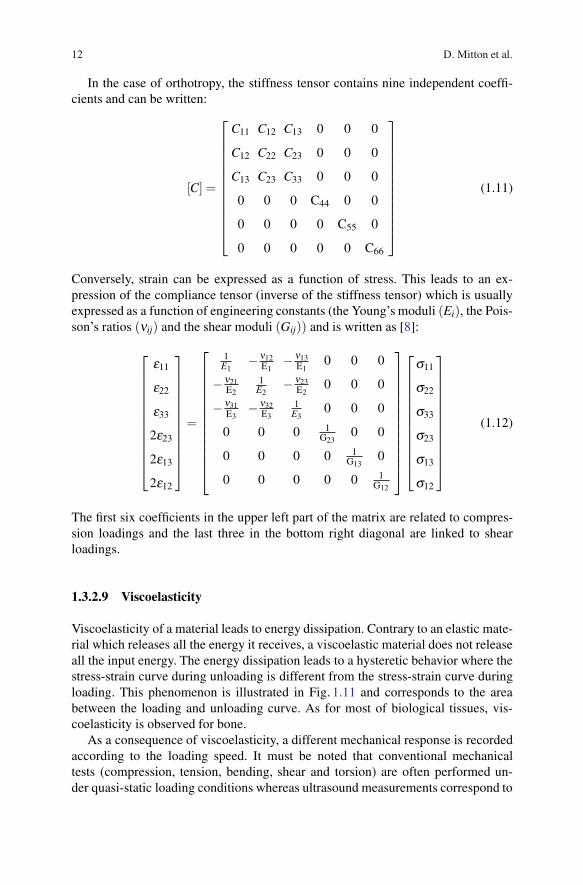
12 D. Mitton et al.

In the case of orthotropy, the stiffness tensor contains nine independent coeffi-cients and can be written:

[C] =

⎡⎢⎢⎢⎢⎢⎢⎢⎢⎢⎢⎢⎣

C11 C12 C13 0 0 0

C12 C22 C23 0 0 0

C13 C23 C33 0 0 0

0 0 0 C44 0 0

0 0 0 0 C55 0

0 0 0 0 0 C66

⎤⎥⎥⎥⎥⎥⎥⎥⎥⎥⎥⎥⎦

(1.11)

Conversely, strain can be expressed as a function of stress. This leads to an ex-pression of the compliance tensor (inverse of the stiffness tensor) which is usuallyexpressed as a function of engineering constants (the Young’s moduli (Ei), the Pois-son’s ratios (νij) and the shear moduli (Gij)) and is written as [8]:

⎡⎢⎢⎢⎢⎢⎢⎢⎢⎢⎢⎢⎣

ε11

ε22

ε33

2ε23

2ε13

2ε12

⎤⎥⎥⎥⎥⎥⎥⎥⎥⎥⎥⎥⎦

=

⎡⎢⎢⎢⎢⎢⎢⎢⎢⎢⎢⎢⎢⎣

1E1

− ν12E1

− ν13E1

0 0 0

− ν21E2

1E2

− ν23E2

0 0 0

− ν31E3

− ν32E3

1E3

0 0 0

0 0 0 1G23

0 0

0 0 0 0 1G13

0

0 0 0 0 0 1G12

⎤⎥⎥⎥⎥⎥⎥⎥⎥⎥⎥⎥⎥⎦

⎡⎢⎢⎢⎢⎢⎢⎢⎢⎢⎢⎢⎣

σ11

σ22

σ33

σ23

σ13

σ12

⎤⎥⎥⎥⎥⎥⎥⎥⎥⎥⎥⎥⎦

(1.12)

The first six coefficients in the upper left part of the matrix are related to compres-sion loadings and the last three in the bottom right diagonal are linked to shearloadings.

1.3.2.9 Viscoelasticity

Viscoelasticity of a material leads to energy dissipation. Contrary to an elastic mate-rial which releases all the energy it receives, a viscoelastic material does not releaseall the input energy. The energy dissipation leads to a hysteretic behavior where thestress-strain curve during unloading is different from the stress-strain curve duringloading. This phenomenon is illustrated in Fig. 1.11 and corresponds to the areabetween the loading and unloading curve. As for most of biological tissues, vis-coelasticity is observed for bone.

As a consequence of viscoelasticity, a different mechanical response is recordedaccording to the loading speed. It must be noted that conventional mechanicaltests (compression, tension, bending, shear and torsion) are often performed un-der quasi-static loading conditions whereas ultrasound measurements correspond to

1 Bone Overview 13

σ

ε

Fig. 1.11 Loading-unloading cycle (hysteresis loop) of the stress-strain curve, below the yieldstress. The area between the two curves represents the dissipative energy

Fig. 1.12 Scanning electron microscopy images of loaded trabeculae, (a) microcrack, (b) brokentrabecula

dynamic mechanical testing with high strain rate. This difference is important whencomparing the data obtained by both methods.

1.3.2.10 Strength

The strength of a material is its ability to withstand an applied stress without failure.The ultimate stress gives a quantification of the ultimate strength.

1.3.2.11 Damage

Damage is a degradation of the material. Figure 1.12 shows microcracks and fail-ure of two different loaded bone trabeculae (see Chap. 15 for details on the use ofultrasound to investigate damage in bone tissue).

14 D. Mitton et al.

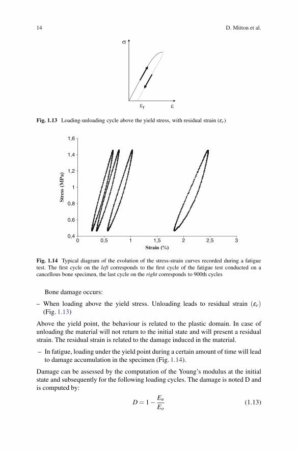
σ

εεr

Fig. 1.13 Loading-unloading cycle above the yield stress, with residual strain (εr)

0,4

0,6

0,8

1

1,2

1,4

1,6

0 0,5 1 1,5 2 2,5 3Strain (%)

Str

ess

(MP

a)

Fig. 1.14 Typical diagram of the evolution of the stress-strain curves recorded during a fatiguetest. The first cycle on the left corresponds to the first cycle of the fatigue test conducted on acancellous bone specimen, the last cycle on the right corresponds to 900th cycles

Bone damage occurs:

– When loading above the yield stress. Unloading leads to residual strain (εr)(Fig. 1.13)

Above the yield point, the behaviour is related to the plastic domain. In case ofunloading the material will not return to the initial state and will present a residualstrain. The residual strain is related to the damage induced in the material.

– In fatigue, loading under the yield point during a certain amount of time will leadto damage accumulation in the specimen (Fig. 1.14).

Damage can be assessed by the computation of the Young’s modulus at the initialstate and subsequently for the following loading cycles. The damage is noted D andis computed by:

D = 1− En

Eo(1.13)

1 Bone Overview 15

where E0 is the Young’s modulus at the initial step and En is the Young’s modulusfor the current loading cycle.

1.3.2.12 Toughness

The toughness of a material is the capability of bone tissue to absorb energy duringthe failure process. It can be assessed from the computation of the energy until fail-ure which is the area under the stress-strain curve up to failure (Fig. 1.7). Fracturemechanics approaches are usually employed. Two parameters are commonly usedfor assessing fracture toughness: critical stress intensity factor (Kc in MPa.

√m) and

critical strain energy release rate (Gc in J.m−2), respectively. The former charac-terizes the stress intensity around the crack tip, whereas the latter is related to thesurface energy of the newly formed crack surfaces [22].

Orders of magnitude of the main parameters that can be assessed for both cor-tical and cancellous bones at the mesoscopic level are presented in Table 1.2. Thelarge variability is due to differences in measurement protocols and to intra or inter-subject variability.

Table 1.2 Mechanical properties of human bone at the mesoscopic level (cortical and cancellousbone)

Cortical boneMean (SD) {Range}

Cancellous boneMean (SD) {Range}

ElasticityYoung’s modulus

(longitudinal, EL)(MPa)

Femoral diaphysis: 14300(400) in tension, 11800(360) in compression [23]17400b [8]

Vertebra: 138 (83)a

Femoral head: 417(85) [24]

Young’s modulus(transverse, ET)(MPa)

9600b [8] Vertebra {16–100}a

Poisson’s coefficient (ν) Femur: 0.22–0.42 [25] Proximal femur: 0.3 [26]Shear modulus (G)

(MPa)3510b [8] Femoral head:

{100–500} [27]

StrengthUltimate stress (MPa) Femoral diaphysis: 53.8 (20.3)

in tension, 106.4 (29.4) incompression [23]

Vertebra: 1.6 (0.9)a

Femoral head: 9.6(2.4) [24]

ToughnessCritical stress intensity

factor (Kc)(MPa.

√m)

Humeral diaphysis: 2.06(0.2) [28]

Femoral head:{0.1–1} [29]

a Mitton, unpublished datab Anatomical site non defined

16 D. Mitton et al.

1.3.3 Elasticity at the Microscopic Level

Young’s modulus can also be assessed at a microscopic level. Apart from acousticmicroscopy that will be detailed in Chap. 16, bone tissue micro-elastic propertiescan be assessed with three methods: (1) traditional mechanical testing (compression,tension and three or four-point bending), (2) micro-computed tomography (μCT)image-based finite-element models and (3) nanoindentation.

1. Traditional mechanical testing already mentioned at the macro- or mesoscopicscales have been adapted to test small specimens. More details can be foundin the references [8, 30]. At the microscopic scale, the difficulties are related tothe small size of the samples that can be prepared from human bones (corticalthickness at some anatomical sites is less than 1 mm and trabeculae thickness isaround 100μm).

2. To overcome these limits the Young’s modulus of bone tissues (cortical andtrabecular) can be assessed by an inverse method using micro finite element mod-elling and biomechanical experiments. Such method is based on imaging such ashigh resolution computed tomography [31–33]. The tissue Young’s modulus isobtained by an optimization routine that matches both the experimental and sim-ulated displacement of the specimen for a given load.

3. Nanoindentation uses a diamond indenter to load and unload a material. TheYoung’s modulus can be derived from the unloading curve [34] (Fig. 1.15).

Table 1.3 shows the variability of the Young’s modulus according the anatomicalsite, the measuring methods. Nanoindentation can assess the spatial heterogeneityof the elastic properties for osteons (22.5± 1.3GPa) and for interstitial lamellae(25.8±0.7) [34] or within lamellae [35].

1.3.4 Synthesis

It is important to note that a large number of investigators have reported a stronglinear relationship between the Young’s modulus and the ultimate compressive

Young’s modulus

Load

Displacement

Fig. 1.15 Typical load-displacement curve for a nanoindention test. The Young’s modulus isderived from the slope of the upper portion of the unloading curve

1 Bone Overview 17

Table 1.3 Elastic properties of human bone tissue at the microscopiclevel (cortical and cancellous tissues)

Values in GPa, mean (SD) {Range}Young’s modulus Cortical tissue Cancellous tissue

Tensile test (tibia) 18.6 (3.5) [36] 10.4 (3.5) [36]Three-point bending

(iliac crest)4.89 [37] 3.81 [37]

Three-point bending(tibia)

5.44 (1.25) [38] 4.59 (1.60) [38]

μCT image-based finiteelement models(proximal tibia)

– {2.23–10.1} [31]

μCT image-based finiteelement models(vertebra)

– 5.7 (1.6) [39]

CT image-based finiteelement models(98 μm pixel size)(radius)

16 (1.8) [19] –

Nanoindentation(femur)

20.02 (0.27) [40] 18.14 (1.7) (distalepiphysis) [40]25.0 (4.3) [41]

6.9 (4.3) (neck) [41]

μCT: micro computed tomography

strength [24, 42]. Moreover, there is also an extremely tight correlation betweenthe Young’s modulus and the bending strength [43]. Thus, Young’s modulus can beused as a surrogate for bone strength. The measurement of the ultrasound propaga-tion velocity (see Chap. 13) that is directly related to the bone stiffness (or to theYoung’s modulus) can also be used as a surrogate measurement for bone strength.

The orders of magnitude of the main mechanical parameters are summarizedin Tables 1.1–1.3. The important variability is due to various factors, includingintra and inter-subjects differences, skeletal sites and experimental protocols.In particular, the macro or mesoscopic mechanical properties (ultimate strength,toughness, fatigue strength) of cancellous and cortical bones decrease with age[44–46]. These modifications are related to an increased porosity and cancellousbone micro-architecture degradation. At the microscopic level the elastic proper-ties are not affected by aging [47]. However collagen crosslinking, collagen fibersorientation, their interaction with bone crystals and water content are modified byaging and are correlated with toughness reduction for cortical bone [22, 48].

To summarise, the influences of the bone composition and structure on its me-chanical properties are the following [49]:

1. The porosity modifies Young’s modulus independently of density2. Microcracks weaken cortical bone tissue and contribute to increased susceptibil-

ity to fracture3. The collagen fibrils provide tensile strength and toughness4. The crystalline structure provides compressive strength and brittleness

18 D. Mitton et al.

1.4 Densitometric and Morphological Parameters

The main densitometric and morphological parameters affecting the mechanicalcompetence of bone are listed Table 1.4. The preferred techniques to measure thesecharacteristics are indicated below.

At the macroscopic scale, the quantitative analysis includes the assessment ofbone mineral density and morphology:

– Bone mineral density (BMD) corresponds to the density of the mineral phase ofthe bone. This density can be measured with X-ray absorptiometry techniques.The mineral phase alone contributes to the images. Because the amount of min-eral is normalized by the total area or total volume occupied by the bone, BMDdoes not represent the true density but rather is an apparent density. BMD can beassessed in vivo using imaging techniques such as:

• Dual X-ray absorptiometry (DXA): DXA is the gold standard method in clin-ics for densitometry measurements. A DXA image is a 2D projection ofthe segment of interest (Fig. 1.16) where both cancellous and cortical boneare superimposed. Thus the density is obtained in g/cm2 and refers to arealbone mineral density (BMDa) [50].

• X-ray quantitative computed tomography (QCT): a certain number ofcross-sections of the anatomical site are reconstructed from QCT acquisi-tions. Volumetric density (g/cm3) (BMD) is derived from volumetric (orthree-dimensional, 3-D) measurements performed using QCT, enabling dif-ferentiation between cortical and cancellous bone densities.

Extensive details on the techniques and the parameters that can be derived fromsuch methods can be found in the International Commission on Radiation Units andMeasurements (ICRU) bone densitometry report [50].

Table 1.4 Main bone structural features determining bone strength,according to physical scale (From [67])

Scale (m) Bone characteristics

>10−2 MacrostructureBone densitiesWhole bone morphology (size and shape)

10−2–10−3 Mesoscopic scale (apparent and real densities)10−6–10−3 Microstructure (porosity, cortical thickness, trabecular

number and spacing, structural anisotropy)10−9–10−6 Sub-microstructure (microcracks)

Nanostructure (collagen fibers)<10−9 Sub-nanostructure (hydroxyapatite crystals)

1 Bone Overview 19

Fig. 1.16 Dual-X-ray Absorptiometry (DXA) images and areas of interest for bone mineraldensity measurement (a) hip and (b) lumbar spine

Fig. 1.17 Example of femoral geometric features derived from 3-D model issued from biplanarradiography (a) neck shaft angle and (b) the femoral neck axis length

– Geometric features (e.g. in the case of the proximal femur: neck shaft angle,femoral neck axis length, cortical thickness of the femoral neck) (Fig. 1.17) canbe derived either using plain radiographic or DXA projection images with po-tential bias due to projection, or in 3-D using biplanar radiography [51, 52] orcomputed tomography [53].

At the mesoscopic scale, bone density can be measured in small bone specimens ofa few millimetres in each dimension by weighting the specimens and by dividing