
Bonds and FX - Booth School of...
59
Bonds and FX Fama-Bliss, Asset Pricing 1. Preview: The basic picture is still “1/p forecasts excess returns” (If you’re not familiar with yields etc., read discrete time bonds chapter) 2. Expectations hypothesis: 1) y (N) t = E t P N−1 j=0 y (1) t+j (+rp, constant over time) 2) f N−1→N t = E t (y (1) t+N−1 ) (+rp, constant over time) 3) y (1) t = E t r N→N−1 t+1 .(+rp, constant over time) You can see a rough truth in the data. But you can also see “sluggish adjustment” which is the core of the predictability result. 1. Facts 1960 1970 1980 1990 2000 2010 5 10 15 Yields of 1-5 year zeros and fed funds 1960 1970 1980 1990 2000 2010 -2 -1 0 1 2 Yield spreads y (n) -y (1) 150
Transcript of Bonds and FX - Booth School of...

Bonds and FX
Fama-Bliss, Asset Pricing
1. Preview: The basic picture is still “1/p forecasts excess returns” (If you’re not familiarwith yields etc., read discrete time bonds chapter)
2. Expectations hypothesis:
1) y(N)t = Et
PN−1j=0 y
(1)t+j (+rp, constant over time)
2) fN−1→Nt = Et(y
(1)t+N−1) (+rp, constant over time)
3) y(1)t = EtrN→N−1t+1 .(+rp, constant over time)
You can see a rough truth in the data. But you can also see “sluggish adjustment” which isthe core of the predictability result.
1. Facts
1960 1970 1980 1990 2000 2010
5
10
15
Yields of 1−5 year zeros and fed funds
1960 1970 1980 1990 2000 2010
−2
−1
0
1
2
Yield spreads y(n)−y(1)
150

1960 1970 1980 1990 2000 2010
2
4
6
8
10
12
14
16
1−5 year forwards
1960 1970 1980 1990 2000 2010
−4
−2
0
2
4
forward spreads f(n)−y(1)
(a) The dominant movement is “level shift” — all yields up and down together.
(b) The yield curve does change shape. Sometimes rising, sometimes falling. This isthe “slope” factor. There is a business cycle pattern: inverted at peaks, rising attroughs.
(c) The pattern since 1987 has been remarkably stable. Poeple who think in termsof monetary policy see a new “stable” regime here.
(d) When the yield/forward curve is upward sloping, interest rates subsequently rise;when yield curve is inverted, interest rates do subsequently fall. The EH looksfairly reasonable.
(e) In 03-04, EH forecast big increases in rates. In 04 and 05 the 1 year rate did rise!Actually 1 year rates rose more than forecast. 5 year rate is dead on the forecast.
151

1 2 3 4 50
1
2
3
4
5yields and forwards
12/03
12/04
12/05
maturity in years
perc
ent
Solid = forward curve. Dash = yield curve.
(f) Risk premium on average? Table 20.8 Update
Interest rate data 1964:01-2008:12Maturity n 1 2 3 4 5E£y(n)
¤6.16 6.37 6.54 6.68 6.76
E£y(n) − y(1)
¤0 0.21 0.38 0.51 0.59
E£r(n) − y(1)
¤0 0.46 0.80 1.38 1.05
σ£r(n) − y(n)
¤0 1.87 3.42 4.73 5.79
“Sharpe” 0 0.25 0.23 0.22 0.18
There does seem to be a small average risk premium for long term bonds. Butit seems small on average. The expectations hypothesis usually means “plus aconstant risk premium” and this is that constant risk premium.
(g) Compare Sharpe to 0.5 of the market portfolio. Long term bonds are way insidethe mean-variance frontier, and β ≈ 0. This makes it a bit of a puzzle why peoplehold them. Actually long-term bonds are the “safe” asset for long term investors,and this is a warning about one-period mean-variance thinking.
(h) Warning: it’s easy to find huge sharpe ratios and “arbitrage” in the term struc-ture; very similar securities with slightly different prices. On/off the run spreads,liquidity spreads, corporate spreads. A bit of a warning, these are a) hard totrade b) hide earthquake risk. Here we’re looking at the basic term spread intreasuries. This may be a pretty boring part! I’ll review these aspects at the end.
152

2. Expectations failures—Fama Bliss. (Updated 1964-2008), table 20.9 update
rx(n)t+1 = y
(1)t+n−1 − y
(1)t =
a+ b³f(n)t − y
(1)t
´+ εt+1 a+ b
³f(n)t − y
(1)t
´+ εt+1
n b σ(b) R2 a b σ(b) R2
2 0.83 0.27 0.12 0.17 0.27 0.013 1.12 0.36 0.13 0.47 0.31 0.044 1.34 0.45 0.14 0.75 0.23 0.125 1.02 0.52 0.06 0.87 0.16 0.16
forecasting one year returns forecasting one year rateson n-year bonds n years from now
3. Wake up. This is the central table.
(a) Left hand panel: “Expected returns on all bonds should be the same” → Run astandard regression to see if anything forecasts the difference in return. Run
r(n)t+1 − y
(1)t = a+ bXt + εt+1
We should see b = 0.
1. Over one year, expected excess returns move one for one with f − s spread!(Should be zero.) The “fallacy of yield” turns out to be correct (at a one yearhorizon).
2. How do we reconcile this with the first table? Long bonds don’t earn muchmore on average. But there are times when long bonds expect to earn more,and other times when they expect to earn less. f − s is sometimes positive,sometimes negative.
(b) Right hand panel, row 1.
1. If f (1→2) is 1% higher than y(1), we should see y(1)t+1 rise 1% higher. We shouldsee b = 1. Instead, we see b = 0! A forward rate 1% higher than the spot rateshould mean the spot rate rises. Instead, it means that the 2 year bond earns1% more over the next year on average.
(c) Right hand panel, higher rows
1. At longer horizons, f − y spread does start to forecast n year changes inyields. (Correspondingly, it ceases to forecast n year returns — not shown.)
2. Once again, expectations does seem to work “in the long run.”
(d) 0.83 + 0.17 = 1 is not by chance. Mechanically, the two coefficients in the firstrow add up. If f − y does not forecast ∆y, it must forecast returns. See the plotof bonds over time for intuition. If we move the p(1)t+1 up we increase expectedreturns r(2)t+1 and decrease the future yield y
(1)t+1.
(e) Note: higher rows do not add up to 1. Why? There are “complementary” regres-sions that add up to 1, I just didn’t show them.
153

Time
PriceHigher 1 year
rate in year 1-2
= lower return of 2 year bond in 0- 1
Time
=Higher 1 yearrate in 3-4
Lower return of 4 year bond from 0-3
Time
Lower return of 4 year bond from 0-1
= Higher 3 yearrate in 1-4
‘safe’ 1 year return
(f) The algebra: As we did before, start with an identity (exact this time)³r(2)t+1 − y
(1)t
´+³y(1)t+1 − y
(1)t
´= f
(2)t − y
(1)t
Proof: Note that the forward-spot spread equals the change in yield plus the excessreturn on the two year bond.
f(1→2)t − y
(1)t = p
(1)t − p
(2)t + p
(1)t
=³p(1)t+1 − p
(2)t + p
(1)t
´+³−p(1)t+1 + p
(1)t
´=
³r(2)t+1 − y
(1)t
´+³y(1)t+1 − y
(1)t
´Hence, when we project down on to f (2) − y(1), and inventing some notation,
b(2)r + b(1)y = 1
In this precise way, a forward rate higher than the spot rate must imply a highreturn on two year bonds or an increase in the on year rate.
(g) Notice how this is all so much like our dividend yield friends, D/P: (If p.dvaries) ∆d should be forecastable so that R not. Fact: ∆d is not forecastable, soR is. Here, (if the yield curve varies) ∆y should be forecastable so r not. Fact:
154

∆y is not forecastable, so r is. We also split variation in the dividend yiled to twoterms by identity and deduced that two regression coefficients must add up,
pt − dt =∞Xj=1
ρj−1 (∆dt+j − rt+j)
blrr − blrd = 1
Here too we had a “complementary regressions” this is just like the D column ofreturn forecasts.
4. Q: Why do we run y(1)t+1 − y
(1)t on f
(2)t − y
(1)t ? The EH says f
(1→2)t = Et
hy(1)t+1
i, so why
not run y(1)t+1 on f
(1→2)t ?
A: That’s valid but not as strong a test. An analogy: Tempt+1 = 0 + 1×Tempt + εt+1works pretty well, so just reporting Tempt makes you look like a good forecaster!But this won’t work for (Tempt+1−Tempt). Being able to forecast changes is a morepowerful test than being able to forecast levels of a slow-moving series like temp, oryield. In short, there’s nothing wrong with doing it with levels, but differences is amore powerful test.
5. Interpretation.
(a) This is like D/P that forecasts returns, not dividend growth. (f − y forecastsreturns, not yield growth.) Variation in D/P must be due to returns of dividendgrowth. (f − y must either forecast yield changes or returns.) Surprise in bothcases: it’s due to returns.
(b) “Sluggish adjustment.” For stocks on D/P; bonds on F-S and exchange rates ondomestic-foreign interest rate, an expected offsetting adjustment doesn’t happen.
1. Stocks: P/D high? D should rise. It doesn’t. “Buy yield” (“value”).2. Bonds: f − y high? y should rise. It doesn’t (at least for a few years). “Buyyield”
If the current yield curve is as plotted in the left hand panel, the right handpanel gives the forecast of future one year interest rates. This is based on the
155

right hand panel of the above table. The dashed line in the right hand panelgives the forecast from the expectations hypothesis, in which case forwardrates today are the forecast of future spot rates.
(c) There are big risk premia and they vary over time. There are times when youexpect much better returns on long term bonds, and other times when you expectmuch better returns on short term bonds. (An upward sloping yield curve resultsin rising rates, but not soon enough — you earn the yield in the meantime). Whenare these times? Look at the plot! High expected returns in recessions (level reces-sions, not growth rate recessions) Interpretation: Business cycle related variationin risk, expected returns. (γ varies over time). Who wants to hold long-termbonds in the bottom of a recession?
6. ADDITIONS/PROBLEM SETS.
(a) Note Fama Bliss with coefficient = 1 is NOT consistent, since if you iterate youdon’t get one year regresisons.
(b) Note the one factor Vasicek does not produce Fama Bliss coefficient.
(c) Result. FB coefficients should be less than one.
Cochrane-Piazzesi 1
Let’s move the question.
Now, let’s ask the question, “what best forecasts returns?” Let’s put all available forwardson the right hand side, not just the maturity-matched pair.
It was right for FF not to do this. Their question was “does the forward spread forecast∆y?”“What causes variation in the right hand side?” (Fama regressions are really about this — whydoes D/P, f-s move?) Also, we’re not really asking, “is the expectations hypothesis right?”That was FB’s motivation. We’re asking, “given it’s wrong, what’s the best characterizationof bond expected returns?”
Motivation 2. (More important) Now we have many right and left hand variables. We needto look for common factors.
r1t+1 = a+ bx1t + ε1t+1r2t+1 = a+ bx2t + ε2t+1
x = f − s for fama bliss, dp vs. f − s looking across stocks and bonds.
a) Does x1 enter equation 2?
b) Maybe
r1t+1 = a+ bx1t + cx2t + ε1t+1r2t+1 = a+ 2bx2t + 2cx
2t + ε2t+1
If so the expected returns are perfectly correlated.
156

What is the factor structure in expected returns?
We want to ask this question across all asset classes. Asking across bond maturities is thestart.
Cochrane-Piazzesi update
Bottom line
1. Forecast 1 year treasury bond returns, over 1 year rate, using all forwards:
rx(n)t+1 = an + β0nft + ε
(n)t+1
2. R2 up to 44%, up from Fama-Bliss / Campbell Shiller 15%
3. A single “factor” γ0f forecasts bonds of all maturities. High expected returns in “badtimes.”
4. A tent-shaped factor is correlated with slope but is not slope. Improvement comesbecause it tells you when to bail out — when rates will rise in an upward-slope envi-ronment
Basic regression
1 2 3 4 5
−2
0
2
4
Unrestricted
5432
1 2 3 4 5
−2
0
2
4
Restricted
5432
rx(n)t+1 = an + b1y
(1)t + b2f
(2)t + ...+ b5f
(5)t + ε
(n)t+1
157
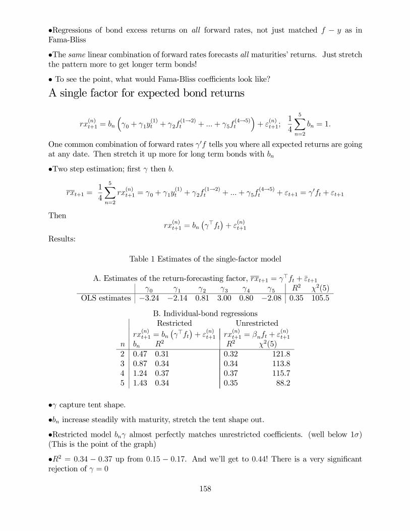
•Regressions of bond excess returns on all forward rates, not just matched f − y as inFama-Bliss
•The same linear combination of forward rates forecasts all maturities’ returns. Just stretchthe pattern more to get longer term bonds!
• To see the point, what would Fama-Bliss coefficients look like?
A single factor for expected bond returns
rx(n)t+1 = bn
³γ0 + γ1y
(1)t + γ2f
(1→2)t + ...+ γ5f
(4→5)t
´+ ε
(n)t+1;
1
4
5Xn=2
bn = 1.
One common combination of forward rates γ0f tells you where all expected returns are goingat any date. Then stretch it up more for long term bonds with bn
•Two step estimation; first γ then b.
rxt+1 =1
4
5Xn=2
rx(n)t+1 = γ0 + γ1y
(1)t + γ2f
(1→2)t + ...+ γ5f
(4→5)t + εt+1 = γ0ft + εt+1
Thenrx
(n)t+1 = bn
¡γ>ft
¢+ ε
(n)t+1
Results:
Table 1 Estimates of the single-factor model
A. Estimates of the return-forecasting factor, rxt+1 = γ>ft + ε̄t+1γ0 γ1 γ2 γ3 γ4 γ5 R2 χ2(5)
OLS estimates −3.24 −2.14 0.81 3.00 0.80 −2.08 0.35 105.5
B. Individual-bond regressionsRestricted Unrestricted
rx(n)t+1 = bn
¡γ>ft
¢+ ε
(n)t+1 rx
(n)t+1 = βnft + ε
(n)t+1
n bn R2 R2 χ2(5)2 0.47 0.31 0.32 121.83 0.87 0.34 0.34 113.84 1.24 0.37 0.37 115.75 1.43 0.34 0.35 88.2
•γ capture tent shape.
•bn increase steadily with maturity, stretch the tent shape out.
•Restricted model bnγ almost perfectly matches unrestricted coefficients. (well below 1σ)(This is the point of the graph)
•R2 = 0.34 − 0.37 up from 0.15 − 0.17. And we’ll get to 0.44! There is a very significantrejection of γ = 0
158

•R2 almost unaffected by the single-factor restriction. The restriction looks good in thegraph.
•See paper version of table 1 for standard errors, joint tests including small sample, unitroots, etc. Bottom line: highly significant; EH is rejected, improvement on FB/3 factormodels is significant.
More lags
1 2 3 4 5−3
−2
−1
0
1
2
3
4
Maturity
Coe
ffici
ent
i=0i=1i=2i=3
rx(n)t+1 = an + b0nft−i + ε
(n)t+1
•More lags are significant, with the same pattern.
•Checking individual lags reassures us it’s not just measurement error, i.e.
pt+1 − pt = a+ bpt + εt+1
if pt is measured with error, you’ll see something. But
pt+1 − pt = a+ bpt−1/12 + εt+1
fixes this problem.
•The pattern suggests moving averages
rxt+1 = a+ γ0 (ft + ft−1 + ft−2 + ...) εt+1
k 1 2 3 4 6R2 0.35 0.41 0.43 0.44 0.43
159

•Interpretation: Yields at t should should carry all information about the future. If the lagsenter, there must be a little measurement error. f change slowly over time, so ft−1/12 isinformative about the true ft. Moving averages are a good way to enhance a slow-moving“signal” buried in high-frequency “noise”.
Stock Return Forecasts
Table 3. Forecasts of excess stock returns (VWNYSE)
rxt+1 = a+ bxt + εt+1
γ>f (t) D/P (t) y(5) − y(1) (t) R2
1.73 (2.20) 0.073.56 (1.80) 3.29 (1.48) 0.08
1.87 (2.38) −0.58 (−0.20) 0.071.49 (2.17) 2.64 (1.39) 0.10
MA γ>f 2.11 (3.39) 0.12MA γ>f 2.23 (3.86) 1.95 (1.02) −1.41 (−0.63) 0.15
• The 5 year bond had b = 1.43. Thus, 1.73− 2.11 is what you expect for a perpetuity.
• It does better than D/P and term spread: Drives out spread; It survives with D/P
• A common term risk premium in stocks, bonds! Reassurance on fads & measurementerrors
• Need to follow up — do impulse responses like I did for cay
History
1965 1970 1975 1980 1985 1990 1995 20000
5
10
−5
0
5
−5
0
5
0
5
Fama−Bliss
γ ′ f
Ex−post returns
Yields
160

• Is it real or just a few data points? What is the story?
•Consistent in many episodes
•γ0f and slope are correlated. Many episodes are interpreted the same way.
•γ0f improvement in many episodes. γ0f says get out in 1984, 1987, 1994, 2004. What’s thesignal?
1 2 3 4 5
2
4
6
8
10
12
14
Dec 1981
Apr 1983
Aug 1985
Apr 1992
Aug 1993Feb 2002Dec 2003
Maturity
For
war
d ra
te (
%)
•Green: CP say buy. Red: FB say buy, CP say don’t.
•Tent-shaped coefficients interact with tent-shaped forward curve to produce the signal.
•CP: in the past, tent-shape often came with upward slope. Others saw upward slope,thought that was the signal. But an upward slope without a tent does not work. The tentis the real signal.
Real time
161

1970 1975 1980 1985 1990 1995 2000
0
5,−5
0
5
10
Full sample
Real time
Regression forecasts γ̂>ft. “Real-time” re-estimates the regression at each t from 1965 to t.(Note: Just because we don’t have data before 1964 doesn’t mean people don’t know what’sgoing on. Out of sample is not crucial, but it is interesting.)
Macro
1965 1970 1975 1980 1985 1990 1995 2000
Return forecastUnemployment
•Is it real, a time-varying risk premium? Or is it some new psychological “effect,” an unex-ploited profit opportunity?
162

• Here, γ0f is correlated with business cycles, and lower frequency. (Level, not growth.)Suggests a “business cycle related risk premium.”
• Also significant that the same signal predicts all bonds, and predicts stocks. If “overlooked”it is common to a lot of markets!
Yield curve factor models.The usual approach: By eigevalue decomposition/factor analysis reduce the yield curve to“level” “slope” and “curvature” factors which explain 99.9% of yield curve variance.
lt = q0lyt; st = q0syt; ct = q0cyt
yt = qllt + qsst + qcct (+εt)
Theorem,QΛQ0 = cov(yty
0t)
the columns of Q provide these numbers.
In this approach, we usually find that st forecasts returns (Fama-Bliss slopes) but with about15% R2
Similar structures come from affine models, which we’ll look at in a bit.
How does the CP γ0ft = γ∗0yt compare to this approach?
1 2 3 4 5−10
−5
0
5
10
15A. Expected return factor γ*
Yield maturity1 2 3 4 5
−0.5
0
0.5level
slope
curvature
B. Yield factors
Yield maturity
1 2 3 4 5−10
−5
0
5
10
15
level, slope,& curve
level & slope
C. Return Predictions
Yield maturity1 2 3 4 5
−2
0
2
4D. Forward rate forecasts
Forward rate maturity
• Top left: γ expressed as an operator for yields not forwards. (Not so pretty, eh?)
163

• Top right: q expressed as a function of yields — how to form factors from yields, andhow yield load on factors.
• Bottom left: what function of level, slope and curve best forecasts returns?
rxt+1 = a+ b(lt) + c(st) + d(ct) + εt+1
Then unwind the factors to find the overall function of yields that best forecasts returns.
Lesson.
1. First smooth, then forecast can throw out the baby with the bathwater. This con-tradicts the usual practice (Stock and Watson) to first find principal components thenforecast. But there was no theory that usual practice was right; maybe the parts thatforecast do not explain much contemporaneous variance.
2. “Maximize variance of yields, returns, etc.” is not “maximize variance of expectedreturns”
3. Expected returns are (nearly) “unspanned state variables” a big new issue in termstructure models.
Failures and spread trades
•What this is about (so far): when, overall is there a risk premium (high expected returns)in long term vs. short term bonds. “Trade” is just betting on long vs. short maturity,“betting on interest rate movements.”
•What this is not about (so far). Much fixed income “arbitrage” involves relative pricing,small deviations from the yield curve. “Trade” might be short 30 year, long 29.5 year.
A hint of spread trades
If the one-factor model is exactly right, then deviations from the single-factor model shouldnot be predictable.
rx(2)t+1 − b2rxt+1 = a(2) + 00ft + εt+1 = a(2) + 00yt + εt+1
(Why?
rx(2)t+1 = α(2) + b2 (γ
0ft) + ε(2)t+1
rxt+1 = α+ γ0ft + ε(2)t+1
multiply the second by b2 and subtract.)
164

Table 7. Forecasting the failures of the single-factor modelA. Coefficients and t-statistics
Right hand variableLeft hand var. const. y
(1)t y
(2)t y
(3)t y
(4)t y
(5)t
rx(2)t+1 − b2rxt+1 −0.11 −0.20 0.80 −0.30 −0.66 0.40
(t-stat) (−0.75) (−1.43) (2.19) (−0.90) (−1.94) (1.68)rx
(3)t+1 − b3rxt+1 0.14 0.23 −1.28 2.36 −1.01 −0.30
(t-stat) (1.62) (2.22) (−5.29) (11.24) (−4.97) (−2.26)rx
(4)t+1 − b4rxt+1 0.21 0.20 −0.06 −1.18 1.84 −0.82
(t-stat) (2.33) (2.39) (−0.33) (−8.45) (9.13) (−5.48)rx
(5)t+1 − b5rxt+1 −0.24 −0.23 0.55 −0.88 −0.17 0.72
(t-stat) (−1.14) (−1.06) (1.14) (−2.01) (−0.42) (2.61)
B. Regression statisticsLeft hand var. R2 χ2(5) σ(γ̃>y) σ(lhs) σ(b(n)γ>y) σ(rx
(n)t+1)
rx(2)t+1 − b2rxt+1 0.15 41 0.17 0.43 1.12 1.93
rx(3)t+1 − b3rxt+1 0.37 151 0.21 0.34 2.09 3.53
rx(4)t+1 − b4rxt+1 0.33 193 0.18 0.30 2.98 4.90
rx(5)t+1 − b5rxt+1 0.12 32 0.21 0.61 3.45 6.00
•This is statistically significant, and this is why GMM rejects the single factor model.
• Pattern: if y(n) is a little out of line with the others (low price), then r(n) is good relativeto all the others.
• No common factor. Bond-specific mean-reversion.
•This is tiny. 17-21 bp, compare to 200-600 bp returns.
•The single-factor γ0f accounts for all the economically important variation in expectedreturns
• But the left hand side is tiny too, so tiny/tiny = good R2
• Tiny isn’t so tiny if you leverage up like crazy!
• But... measurement error looks the same.
Measurement error, φ12 problems, etc.
(See paper.)
Latest data, and treasury curves during the crash
See overheads. This is a real problem. The Fama Bliss data extraction method no longerworks. We need to go back to basic treasury data and do it right.
165

Affine models, background for CP II
Statistical factor model approach
Produces "factor model."
The yield curve is crying for factor structure
1960 1970 1980 1990 2000 2010
5
10
15
Yields of 1−5 year zeros and fed funds
1960 1970 1980 1990 2000 2010
−2
−1
0
1
2
Yield spreads y(n)−y(1)
• Technique: eigenvalue decomposition
Σ = cov(y)
QΛQ0 = Σ;Λ diagonal, Q0Q = QQ0 = I
yt = Qxt; cov(xx0) = Λ→ cov(yy0) = QΛQ0 = Σ
Thus, we get a factor model. The underlying factors x are uncorrelated, ordered byvariance.
1. Λ give us the variances of the "factors"
2. Columns of Q tell us how y loads on x movements, if “factor ‘1 moves” how much doy move. x = Q0yt (cov(x, x0) = Q0ΣQ = Q0QΛQ0Q = Λ)
3. Colums of Q tell us how x is formed from each y, how to construct each factor.
4. (Note “Rotation, identification” There are many different ways to write y = Ax; E(xx0) =D. For example, changing to z1t = x1t/σ1 + x2t/σ2; z2t = x1t/σ1 − x2t/σ2 preserves
166

cov(z1, z2) = 0. The eigenvalue decomposition solves
max var(q0y) s.t. q0q = 1
max var(q20y) s.t. q02q2 = 1, q02q1 = 0
...
Note: identification will be poor if the variance is about the same; small differences inthe sample will produce q that jump between one and the other factor. Often you wantto identify in other ways than by variance ordering, i.e. to get interpretable shapes ofthe loadings. For example, if you do this to the FF 25 portfolios, you get two factors,each of which is a mixture of smb and hml, and nearly the same variance. Rotating tosmb and hml gives a more pleasing structure.)
5. (Note: Unit variance factors
yt = QΛ1/2xt; cov(xtx0t) = I
xt = Λ−12Q0y
Loadings QΛ1/2 are smaller for smaller factors. This is a nice way to show the relativeimportance as well as the shapes of the factors, and not have your readers spend toomuch time interpreting the 5th factor.)
6. λi/P
λi = “fraction of variance explained by ith factor”
• Result, applied to FB yield data
Sigma = cov(100*yields);[Q,L] = eig(Sigma);disp(diag(L)’.^0.5);%(my names)2-5 zigzag curve slope level
0.06 0.07 0.10 0.58 5.80disp(Q)
0.06 0.15 -0.47 -0.74 0.46-0.35 -0.55 0.56 -0.21 0.460.70 0.32 0.44 0.12 0.45-0.59 0.57 -0.03 0.36 0.440.19 -0.49 -0.52 0.51 0.43
loads = Q*L^0.5;plot(loads)plot(Q)
167

1 2 3 4 5−0.5
0
0.5
1
1.5
2
2.5
3loadings with σ = 1
levelslopecurvezigzag2−5
1 2 3 4 5−1
−0.5
0
0.5
1loadings
levelslopecurvezigzag2−5
• “Factor models” come from dropping the small eigenvalues. Then a larger number ofseries are, exactly, driven by a smaller number of factors.
• For example, what if we drop 4 and 5?⎡⎢⎢⎢⎢⎢⎣y(1)t
y(2)t
y(3)t
y(4)t
y(5)t
⎤⎥⎥⎥⎥⎥⎦ ≈ q1 × levelt + q2 × slopet + q3 × curvet
168

1955 1960 1965 1970 1975 1980 1985 1990 1995 2000 2005 20100
0.1
actual yields
1955 1960 1965 1970 1975 1980 1985 1990 1995 2000 2005 20100
0.1
level only
1955 1960 1965 1970 1975 1980 1985 1990 1995 2000 2005 20100
0.1
level and slope
1955 1960 1965 1970 1975 1980 1985 1990 1995 2000 2005 20100
0.1
level, slope and curve
2000 2001 2002 2003 2004 2005 2006 20070.01
0.02
0.03
0.04
0.05
0.06
0.07levels only
169

2000 2001 2002 2003 2004 2005 2006 20070.01
0.02
0.03
0.04
0.05
0.06
0.07level and slope
2000 2001 2002 2003 2004 2005 2006 20070.01
0.02
0.03
0.04
0.05
0.06
0.07level slope and curve
Movements in yields can be captured very well by movements in the first two - threefactors alone. But not exactly!
• Dropping factors II. Note that the factors are uncorrelated with each other. cov(xx0) =Λ. Thus, the left out factors are uncorrelated with the factors you keep in.
y(n)t ≈ q
(n)1 × levelt + q
(n)2 × slopet + q
(n)3 × curvet + (left outt)
170

Therefore, this is a regression equation! This is a way of finding a regression modellike FF3F when you don’t know what to use on the right hand side.
• Notice the analogy to FF3F: three factors (market, hml, smb) account for almost allreturn variation (R2 above 90%). The factors are constructed as weighted combinationsof the same securities.
Motivation for term structure models
1. Let’s simplify for a bit to an exact factor model,
y(n)t ≈ q
(n)1 × levelt + q
(n)2 × slopet + q
(n)3 × curvet
It suggests a simple description of the yield curve, boil it all down to
Xt =£lt st ct
¤0Xt+1 = μ+ ΦXt + εt+1
yt(N × 1) = q(N × 3)Xt(3× 1)
2. But
(a) Can you extend this to other maturities, not included? Since there are 3 factors,spanned, there is only one arbitrage-free extension. Can you extend to options —which must also be a function of X?
(b) The point of most affine models: Like Black and Scholes, find an arbitrage-freeinterpolation and extension. For B-S, it was (stock, bond -> option) For us, itis from a few bonds to all maturities, and then to term structure options, whosevalue only depends on the current yield curve and can be replicated by dynamictrading of bonds.
(c) Note: if all you care about is running an arbitrage-free curve through today’s bonds(and options) you don’t care about risk premia. You don’t care about the realmeasure; do everything under risk neutral measure. But then ignore forecasting.Real vs. risk neutral measure only matters if you care about forecasting.
Term structure models
Note to self: Needs a consistent notation once and for all with my model with piazzesi. Userisk neutral notation for expectations model.
Macro approach
P(N)t = Et
µβN
u0(ct+N ,mt+N)
u0(ct)
171

1. Just test
2. Model
Xt =
⎡⎣ ctx2tx3t
⎤⎦ ;Xt+1 = ΦXt + εt+1;
compute P (N)t ?
(a) Won’t be equal to exact P (N)t
(b) Agents see more than we do, maybe P (N)t should be in X?
3. Useful for “deep explanation,” but there are other uses...This is more than we need forthe “arbitrage-free extension” project.
Expectations hypothesis model
This is the simplest “model” to illustrate the logic. The ingredients are a) short rate processb) expectations to get other prices
y(1)t+1 − δ = φ(y
(1)t − δ) + εt+1
f(2)t = Et(y
(1)t+1) = δ + φ(y
(1)t − δ)
f(3)t = Et(y
(1)t+2) = δ + φ2(y
(1)t − δ)
f(N)t = Et(y
(1)t+N−1) = δ + φN−1(y
(1)t − δ)
(And yields,...)
y(2)t =
1
2
hEt(y
(1)t+1) + y
(1)t
i=
1
2
hδ + φ(y
(1)t − δ) + y
(1)t
iy(2)t − δ =
1 + φ
2
³y(1)t − δ
´...
y(N)t − δ =
1 + φ+ φ2 + ..
N
³y(1)t − δ
´=
1− φN
N(1− φ)
³y(1)t − δ
´Result:
1. Different shapes of the term structure, upward and downward sloping. Up when shortrates expected to rise.
2. More complex shapes? Move past AR(1)!
172

3. A “one factor model” of the yield curve. We obviously could generalize to “multifactor”with a more complex time-series process.∙
x1tx2t
¸= Xt
Xt = ΦXt−1 + εt
y(1)t = δ0 + δ01Xt
4. No average slope — E(y(i)) all the same. Well, we imposed expectations!
5. “Arbitrage?” We’re almost there. If the expectations model were the risk neutrallimit, then we could appeal to the risk neutral density theorem and claim these arearbitrage-free prices under the risk neutral density. Alas, they’re not..
Discrete-time single-factor Vasicek
Here: A standard “single factor model” — “discrete-time Vasicek.” The end result:³y(1)t+1 − δ
´= φ
³y(1)t − δ
´+ vt+1.
f(2)t = δ + φ
³y(1)t − δ
´−∙1
2+ λ
¸σ2ε
f(3)t = δ + φ2
³y(1)t − δ
´−∙1
2(1 + φ)2 + λ(1 + φ)
¸σ2ε
....
y(2)t = δ +
(1 + φ)
2
³y(1)t − δ
´− 12
µ1
2+ λ
¶σ2ε
y(3)t = δ +
(1 + φ+ φ2)
3
³y(1)t − δ
´− 13
½1
2
£1 + (1 + φ)2
¤+ λ [1 + (1 + φ)]
¾σ2ε
....
Intuition for now: the first equation tells you where interest rates are going over time. Thesecond and third sets of equations tell you where each forward rate is at any date, dependingonly on where the short rate is on that date; a single factor model.
Derivation:
• Suppose m follows the time series model.
xt+1 − δ = φ (xt − δ) + εt+1
mt+1 = lnMt+1 = −1
2λ2σ2ε − xt − λεt+1
This is just a model for m, with a convenient “state variable” xt. Intuition: xt shiftsthe mean of lnmt+1 around. If you remember that Rf = 1/E(m), you can see that
173

specifying a model for the mean of m is the key to thinking about interest rates. The1/2σ2 term just shifts the mean of lnmt down, and offsets a 1/2σ2 term which willpop up later. To be specific, ε and v are iid Normal with σ2ε, σ
2v, σεv. δ, ρ, λ are free
parameters; we’ll pick these to make the model fit as well as possible.
• An interpretation:
xt+1 − δ = φ (xt − δ) + εt+1
∆ct+1 =1
γ
µ−δ + xt +
1
2λ2σ2ε + λεt+1
¶→ −δ − γ∆ct+1 = −xt −
1
2λ2σ2ε − λεt+1
“suppose consumption growth followed this ARMA (1,1) process, but we didn’t observeconsumption growth. Like all finance (CAPM etc) ultimately we’re abstracting awaythe connection to macro. Obviously, if we want to “explain” asset prices, we need toput back in tne connection to macro!
• Bond prices.P(n)t = Et (Mt+1Mt+2....Mt+n)
This is easier to do recursively,
P(0)t = 1
P(n)t = Et
³mt+1P
(n−1)t+1
´.
• Here we go.P(1)t = Et (Mt+1) = Ete
mt+1
P(1)t = e−
12λ2σ2ε−xt+ 1
2λ2σ2ε = e−xt
p(1)t = lnEt (mt+1) = −xty(1)t = xt
Now you see why I set up the problem with the 1/2λ2σ2ε to begin with! The one yearinterest rate “reveals the latent state variable x t”
• I could have written the model as
y(1)t+1 − δ = φ
³y(1)t − δ
´+ εt+1
mt+1 = −y(1)t −1
2λ2σ2ε − λεt+1
“a short rate process plus a market price of risk.” Then, by taking − lnEt (Mt+1) Iwould have checked that the y(1)t the model produces is the same y(1)t I started with.Take your pick. Which is more confusing: a) starting with an xt you “can’t see” andthen showing that it turns out to be y(1)t ? b) starting with an assumed y
(1)t process and
then showing that it’s in fact the one period rate, that the model is “self-consistent”(in the language of CP appendix.)
174

• On to the next price.
P(2)t = Et
³mt+1P
(1)t+1
´= Et
³emt+1+p
(1)t+1
´= Et
³e−
12λ2σ2ε−xt−λεt+1−xt+1
´P(2)t = Et
³e−
12λ2σ2ε−xt−λεt+1−δ−φ(xt−δ)−εt+1
´P(2)t = Et
³e−2δ−(1+φ)(xt−δ)−
12λ2σ2ε−(1+λ)εt+1
´p(2)t = −2δ − (1 + φ) (xt − δ)− 1
2λ2σ2ε +
1
2(1 + λ)2σ2ε
p(2)t = −2δ − (1 + φ) (xt − δ) + (
1
2+ λ)σ2ε
• From prices, we find yields and forwards,
y(2)t = δ +
(1 + φ)
2(xt − δ)− 1
2
µ1
2+ λ
¶σ2ε
f(2)t = p
(1)t − p
(2)t
= −δ − (xt − δ) + 2δ + (1 + φ) (xt − δ)− (12+ λ)σ2ε
= δ + φ (xt − δ)− (12+ λ)σ2ε
• Now the rest of the maturities. You can “solve the discount rate forward and integrate”p(3)t = logEt (Mt+1Mt+2Mt+3)
p(3)t = logEte
− 12λ2σ2ε−xt−λεt+1− 1
2λ2σ2ε−xt+1−λεt+2− 1
2λ2σ2ε−xt+2−λεt+3
= logEte−3δ− 3
2λ2σ2ε−(1+φ+φ2)(xt−δ)−λεt+1−λεt+2−λεt+3−(1+φ)εt+1−εt+2
This will work after much algebra
• Instead, let’s do it recursively “derive a differential equation for price as a function ofstate variables.” Guess
P(n)t = An −Bn (xt − δ)
thenP(n)t = Et
³Mt+1P
(n−1)t+1
´(Not in lecture:
An −Bn (xt − δ) = logEt
µexp
µ−12λ2σ2ε − xt − λεt+1
¶exp (An−1 −Bn−1 (xt+1 − δ))
¶= logEt
µexp
µ−12λ2σ2ε − xt − λεt+1 +An−1 −Bn−1φ (xt − δ)−Bn−1εt+1
¶¶= logEt
µexp
µ−δ +An−1 − (1 +Bn−1φ) (xt − δ)− 1
2λ2σ2ε − λεt+1 −Bn−1εt+1
¶An −Bn (xt − δ) = −δ +An−1 − (1 +Bn−1φ) (xt − δ) +
µBn−1λ+
1
2B2n−1
¶σ2ε
175

The constant and the term multiplying xt must separately be equal. Thus,
Bn = 1 +Bn−1φ
An = −δ +An−1 +
µBn−1λ+
1
2B2n−1
¶σ2ε
We have “transformed the solution of a stochastic differential equation plus integral tothe solution of an ordinary differential equqation.
• That’s easy to solve
B0 = 0
B1 = 1
B2 = 1 + φ
B3 = 1 + φ+ φ2
Bn =n−1Xj=0
φj =1− φn
1− φ
A0 = 0
A1 = −δ
A2 = −2δ +µλ+
1
2
¶σ2ε
A3 = −3δ +∙(1 + φ)λ+
1
2(1 + φ)2
¸σ2ε
A4 = −4δ +∙¡1 + φ+ φ2
¢λ+
1
2
¡1 + φ+ φ2
¢2¸σ2ε
You see the pattern from here
• Yields, forwards, returns, etc. follow. y(n)t = −1/n× p(n)t . Forwards are even simpler,
f(n)t = p
(n−1)t − p
(n)t
= (An−1 −An)− (Bn−1 −Bn) (xt − δ)
= −δ +µBn−1λ+
1
2B2n−1
¶σ2ε + φn−1 (xt − δ)
• Result: ³y(1)t+1 − δ
´= φ
³y(1)t − δ
´+ εt+1.
f(2)t = δ + φ
³y(1)t − δ
´− (12+ λ)σ2ε
f(3)t = δ + φ2
³y(1)t − δ
´−∙1
2(1 + φ)2 + λ(1 + φ)
¸σ2ε
f(4)t = δ + φ3
³y(1)t − δ
´−∙1
2
¡1 + φ+ φ2
¢2+ λ(1 + φ+ φ2)
¸σ2ε
...
176

y(2)t = δ +
(1 + φ)
2
³y(1)t − δ
´− 12
µ1
2+ λ
¶σ2ε
y(3)t = δ +
(1 + φ+ φ2)
3
³y(1)t − δ
´− 13
½1
2
£1 + (1 + φ)2
¤+ λ [1 + (1 + φ)]
¾σ2ε
...
1. Just like EH but we now see a now a risk premium emerge!
2. Shapes: A steady decline from σ2 terms, (risk premim) + exponential decay fromy(1) −E(y(1)). (expectations hypothesis)
3. “Short rate process” plus “one factor model.” All yields move in lockstep indexedby y(1)t (or any other yield). The shape is tied to the level. It looks like “you canprice other bonds by arbitrage” but that is only because we restrict our modelto have one factor. “Arbitrage free” pricing in the term structure always comesdown to the assumption that there is a perfect factor structure
4. y(1) is also sufficient to forecast all yields.
5. The risk premium comes from cov(m, y(1)) = λσ2ε “market price of interest raterisk”. If there were a security whose payoff were εt+1 its price would be driven bycov(m, εt+1).
6. The premium can go either way depending on the sign of λ. My guess: lowery(1)t+1means higher m (bad state) means + (m = ..−ε) sign and negative premium.This is a typical result. The real term structure ought to slope down, as long termbonds are safer for long-term investors. However, as long as we separate marketprices of risk from consumption and interest data (as we did with the CAPM!)we can incorporate an upward sloping yield curve with λ < 0
7. The risk premium is constant over time though — as we’ll see not in data.
8. “Risk neutrality” λ = 0 does not mean “expectations” since there is another term.This is Another force for typical downward slope. However, it’s quantitatively verysmall, since σε ≈ 0.01
9. Another way to see risk premia is to look at returns,
r(n)t+1 = p
(n−1)t+1 − p
(n)t = (An−1 −An)−Bn−1 (xt+1 − δ) +Bn (xt − δ)
= δ −µBn−1λ+
1
2B2n−1
¶σ2ε −Bn−1 (xt+1 − δ) +Bn (xt − δ)
Expected returns
Etr(n)t+1 = δ −
µBn−1λ+
1
2B2n−1
¶σ2ε + (Bn −Bn−1φ) (xt − δ)
Etr(n)t+1 = δ −
µBn−1λ+
1
2B2n−1
¶σ2ε + (xt − δ)
Etrx(n)t+1 = −
µBn−1λ+
1
2B2n−1
¶σ2ε
You see the expected returns differ by maturity, but the risk premium is constantover time — not what Fama-Bliss find.
177

10. The limiting yield and forward rate are constants. There is no true “level” shift.We’ll see this is quite general — “level shifts” imply an arbitrage opportunity atthe long end of the yield curve.
11. Yields can be negative — they are normally distributed here. M > 0 means P > 0not P < 1. The CIR model fixes this up.
12. As a reminder, ³y(1)t+1 − δ
´= φ
³y(1)t − δ
´+ εt+1.
f(2)t = δ + φ
³y(1)t − δ
´− (12+ λ)σ2ε
Now, suppose you write a new model with³y(1)t+1 − δ∗
´= φ
³y(1)t − δ∗
´+ εt+1.
with a new and different mean,
δ∗ = δ − σ2ε1− φ
λ
and then you set λ = 0. You’d get
f(2)t =
µδ − σ2ε
1− φλ
¶+ φ
µy(1)t −
µδ − σ2ε
1− φλ
¶¶−µ1
2
¶σ2ε
f(2)t = δ + φ
³y(1)t − δ
´− σ2ε1− φ
λ+ φσ2ε1− φ
λ−µ1
2
¶σ2ε
f(2)t = δ + φ
³y(1)t − δ
´− 1− φ
1− φσ2ελ−
µ1
2
¶σ2ε
f(2)t = δ + φ
³y(1)t − δ
´−µ1
2+ λ
¶σ2ε
the same thing! “Transform to risk-neutral probabilities which alter the drift,then use risk-neutral valuation formula” We can write the whold model this way.
f(2)t = δ∗ + φ
³y(1)t − δ∗
´− (12)σ2ε
f(3)t = δ∗ + φ2
³y(1)t − δ∗
´−∙1
2(1 + φ)2
¸σ2ε
f(4)t = δ∗ + φ3
³y(1)t − δ∗
´−∙1
2
¡1 + φ+ φ2
¢2¸σ2ε
Advantage: prettier formula. Disadvantage: can’t describe real dynamics — don’tfit the first equation by running a regression of y(1)t+1 on y
(1)t
• Let’s see an example.
178

1. I chose some parameters to fit the FB zero coupon bond data. I ran a regressionof y(1)t+1 on y
(1)t to get ρ; I took the variance of errors from that regression to get
σε; I took the mean δ = E³y(1)t
´. Finally, I picked the market price of risk λ to
fit the average 5 year forward spread:
f(5)t = δ + φ4
³y(1)t − δ
´−∙1
2
¡1 + φ+ φ2 + φ3
¢2+ λ(1 + φ+ φ2 + φ3)
¸σ2ε
λ = −E³f(5)t
´− δ
(1 + φ+ φ2 + φ3)σ2ε− 12
¡1 + φ+ φ2 + φ3
¢2. I plot y(n)t for a bunch of y(1)t . The dashed lines in the right hand graph give theexpectations hypothesis terms from above, so you can see the distortion from riskaversion λ and the Jensen’s inequatlity σ2ε term.
0 2 4 6 8 100
0.02
0.04
0.06
0.08
0.1
maturity
perc
ent
forwards, λ = −13.2, ρ = 0.84, 100 x σ = 1.58
0 2 4 6 8 100
0.02
0.04
0.06
0.08
0.1
maturity
perc
ent
forwards and expectations
0 2 4 6 8 100
0.02
0.04
0.06
0.08
0.1
maturity
perc
ent
yields
0 2 4 6 8 100
0.02
0.04
0.06
0.08
0.1
maturity
perc
ent
yields and expectations
Cool! This captures some basic patterns; yields are upward sloping when lower,downward sloping when higher. The substantial risk premium I estimated tomatch the average upward slope does introduce a substantial deviation of themodel from expectations at the long end.
3. Note already: the parameters φ, λ can be chosen to match the cross section ofyields — the shapes of these curves — or the time series — the AR(1) coefficient ofthe short rate and the expected bond returns. These do not necessarily give thesame answer, a sign of model misspecification.
4. Take the history of y(1)t . Find the model-implied y(n)t : compare with data.
179

1955 1960 1965 1970 1975 1980 1985 1990 1995 2000 2005 20100
5
10
15
yiel
ds
Simulation of Vasicek yield model
1955 1960 1965 1970 1975 1980 1985 1990 1995 2000 2005 20100
5
10
15
yiel
ds
1−5 year zero coupon yields
5. You can see a decent fit — upwward sloping yields when the interest rate is low.But you can see yields are going up to a constant long-term value, rather thansome sort of “local mean. This is clearer if we plot spreads,
1955 1960 1965 1970 1975 1980 1985 1990 1995 2000 2005 2010
−2
−1.5
−1
−0.5
0
0.5
1
1.5
Simulation of Vasicek yield spreads
yiel
d sp
read
1955 1960 1965 1970 1975 1980 1985 1990 1995 2000 2005 2010
−2
−1
0
1
2
yiel
d sp
read
1−5 year zero coupon yield spreads
180

Answer: we need a two-factor model....
Cochrane-Piazzesi 2
1. Our original motivation: How do you forecast rates? How much of f(n)t is Ety
(1)t+n−1?
(We were tasked with, examine the “conundrum,” a period in which long term forward rateswere anomalous. Task: Understand rates in 2005. Why were long term rates not rising whenshort term rates rose? Greenspan, “Conundrum” that risk premia seemed to be falling. Us:you must be kidding that you can measure risk premia so well! But let’s try. It seems sosimple — use all rates to forecast Ety
(1)t+n−1, then the residual isk the risk premium)
1990 1991 1992 1993 1994 1995 19962
4
6
8
10
1051ff
2000 2001 2002 2003 2004 2005 20060
2
4
6
8
1051ff
Forward rates in two recessions. The federal funds rate, 1-5, 10 and 15 year forward ratesare plotted. Federal funds, 1, 5 and 10 year forwards are emphasized. The vertical lines in
the lower panel highlight specific dates that we analyze more closely below.
Or is it so easy? VARs leave huge uncertainty about Ety(1)t+5. In addition to wide standard
errors, there is a lot of specification uncertainty. Interest rates have a root close to one, and0.98 vs. 0.99 makes a huge difference. The graph: Ety
(1)t+j based on a VAR using 5 yields at
each date. Top:ft+1 = μ+ Φft + εt+1.
Bottom:∆f
(n)t+1 = μn +
Xm
φn,m
³f(m)t − y
(1)t
´+ ε
(n)t+1
181

1975 1980 1985 1990 1995 2000 20050
5
10
15
VAR in levels
1975 1980 1985 1990 1995 2000 20050
5
10
15
VAR in differences
1. Can we use the structure of a term structure model to learn about the time series fromthe cross section?
(a) Well, f (n)t = E∗(y(1)t+n) but obviously (!) we can’t learn about E without saying
something about risk premiums. Most basically ptu0(ct) =
Pstates πsβu
0(cs)xs;probability and marginal utility always enter jointly.
(b) But we just learned a lot about risk premiums! Can this inform the effort?
2. “Affine model with risk premium.” Another objective: learn about longer-run dynamicsthan the one-year regressions in CP1.
(a) What’s Etr(n)t+2?
(b) Get back to “implications for prices”, feed risk premia through some sort of presentvalue model
3. This is not the usual point of affine model. Usually the point is just to fit the crosssection. In particular, to price an extra security in terms of given securities. (As Blackscholes prices an option in terms of stocks and bonds.) Many authors of affine modelslose sight of this.
4. (Digression: affine models are just waking up to the fact that it is very hard to hedgebond options with bonds. This is the heart of the “unspanned stochastic volatility”
182

message. JC suggestion: well, then you should be hedging one bond option with otherbond options, not with treasuries! A suggestion: create something like affine modelsthat span through a basis set of simple bond options. These will reveal volatility muchbetter than bond prices.)
5. (Note: Point to second to last graph of Dec 30 2007. All yield curve models havetrouble with data below a year. Plug piazzesi’s thesis.)
2. Affine model summary
Xt =£xt levelt slopet curvet
¤0.
Xt+1 = μ+ φXt + vt+1; E¡vt+1v
0t+1
¢= V,
Mt+1 = exp
µ−δ0 − δ01Xt −
1
2λ0tV λt − λ0tvt+1
¶λt = λ0 + λ1Xt.
(A bit of why; we need σt(M) to generate Et(Re)/σt(R
e) that varies over time )
p(n)t = logEt (Mt+n)
Here we gop(1)t = e−δ0−δ
01Xt
y(1)t = δ0 + δ01Xt
This identifies δ0 and δ1. (You can also take the short rate as a factor in X, which makesthe model simpler. We chose not to)
p(2)t = logEt
³e−δ0−δ
01Xt− 1
2λ0tV λt−λ0tvt+1e−δ0−δ
01(μ+φXt+vt+1)
´= logEt
³e−2δ0−δ
01μ−δ01(I+φ)Xt− 1
2λ0tV λt−(λ0t+δ01)vt+1
´= −2δ0 − δ01μ− δ01 (I + φ)Xt + δ01V δ1 − 2δ01V λt= −2δ0 − δ01μ− δ01 (I + φ)Xt +
1
2δ01V δ1 − δ01V (λ0 + λ1Xt)
= (·)− δ01 (I + φ)Xt − δ01V λ01Xt
f(2)t = p
(1)t − p
(2)t = −δ0 − δ01Xt − [(·)− δ01 (I + φ)Xt − δ01V λ1Xt]
= (·) + δ01 (φ− V λ1)Xt
....
f(n)t = ..+ δ01φ
∗(n−1)Xt
φ∗ ≡ φ− V λ1
183

(Note that since f is a linear function of X and X is an AR(1), this model is homoskedasticfor yields and returns. It’s interesting to add conditional variance. However, conditionalvariances in the data are not nearly so simple as the CIR model (variance rises with the levelof rates) predicts; variance is also pretty clearly not well spanned by current yields. If youforecast r2t+1 with past yields and with lagged r2t the latter enter. This is the “unspannedstochastic volatility” observation. In my view, understanding volatility is as ripe for pluckingas understanding means was for Piazzesi and I. Start by forecasting r2t+1 with all f , What’sthe factor structure? Then see if r2t enters.... A lot of regressions and plots could get pastthe mess of the big ML crowd just as our regressions did)
3. We find φ∗
From the cross section (nonlinear regression) Note OLS (f (n)t = ..+ b0nXt) is as good as youcan get.
minPT
t=1
PNn=1
nf(n)t −
h(·) + φ∗(n−1)Xt
io2interpret as measurement errors. Note the model
predicts exact factor structure, so it’s easy to “reject.”
This uses no “time-series information,” there is no (zt+1 − awt)2 (z,w stand for anything) in
this.
In our case, the factors X are “observable.” However, you can also think of them as “latent.”Then, for any guess of φ∗ you use the first N f (n) to back out the X, then use the remainingf (n) to assess the fit of that φ∗ (Of course you do this more intelligently, i.e. for any φ∗ usethe first four degrees of freedom of f (n).)
0 5 10 15 20−0.02
−0.015
−0.01
−0.005
0
0.005
0.01
0.015
Maturity
Loading Bf on x
Risk−neutral modelf on X regression
0 5 10 15 200
0.05
0.1
0.15
0.2
0.25
0.3
0.35Level
Maturity
0 5 10 15 20−0.8
−0.6
−0.4
−0.2
0
0.2
0.4
0.6Slope
Maturity0 5 10 15 20
−0.6
−0.4
−0.2
0
0.2
0.4curve
Maturity
Affine model loadings, Bf in f (n) = Af +Bf 0Xt. The line gives the loadings of the affinemodel, found by searching over parameters δ0, δ1, μ∗, φ
∗. The circles give regressioncoefficients of forward rates on the factors.
184

4. To φ, forecasting? Alas, knowing φ∗ tells you nothing about φ.
Theorem: ∀φ∗, φ,∃λ1 : φ∗ ≡ φ− V λ1
Proof:λ1 = V −1 (φ− φ∗)
Interpretation: The cross section says nothing about the time series without restrictions onmarket prices of risk. ( “A New Perspective on Gaussian DTSMs’ Scott Joslin , Kenneth J.Singleton and Haoxiang Zhu”)
5. But we know a lot about λ from CP1!
Data: Et
³rx
(n)t+1
´= bn (γ
0ft) = bnxt
Model: Et (rxt+1) = (·) + cov(rxt+1, v0t+1) (λ0 + λ1Xt)
(Why? Mt+1 = exp¡−δ0 − δ01Xt − 1
2λ0tV λt − λ0tvt+1
¢1 = Et(MR) = Et
he−δ0−δ
01Xt− 1
2λ0tV λt−λ0tvt+1ert+1
i...)
λ1 columns: how does the risk premium vary over time — which state variables tell you thatEtrxt+1 is higher at time t than it was at time t-1?
λ1Rows: expected returns depend on covariance of returns with what factor?
• The lesson of CP1 is that all variation through time in market prices of risk is carriedby xt
λt = (λ0 + λ1Xt) =
⎡⎢⎢⎢⎣λ(x)0
λ(level)0
λ(slope)0
λ(curve)0
⎤⎥⎥⎥⎦+⎡⎢⎢⎢⎣
λ(x,x)1 0 0 0
λ(l,x)1 0 0 0
λ(s,x)1 0 0 0
λ(c,x)1 0 0 0
⎤⎥⎥⎥⎦⎡⎢⎢⎣
xtleveltslopetcurvet
⎤⎥⎥⎦• So, what covariances to ER line up with?
Et
³rx
(n)t+1
´= (·) + cov(rx
(n)t+1, v
0t+1) (λ0 + λ1Xt)
bnxt = cov(rx(n)t+1, v
xt+1)λ
(x,x)1 xt + cov(rx
(n)t+1, v
lt+1)λ
(l,x)1 xt + ...
bn = cov(rx(n)t+1, v
xt+1)λ
(x,x)1 + cov(rx
(n)t+1, v
lt+1)λ
(l,x)1 + ...
bn become the “expected returns” to match. (we’re matching not “expected returns”but expected returns conditional on X, i.e. x) The right hand side is a multiple-betamodel, with λ as market prices of risk. We want to run a multiple “cross-sectional”regression of bn on cov(rx(n), vi) and see which covariances line up with the expectedreturns. This is just like Fama - French who look at which betas (h, say) line up withexpected returns.
• Visually, you want to know which linear combination of the colored lines add up to theblack squares. It’s all the green line!
185

2 3 4 5 6 7 8 9 10 11 12 13 14 15
qr
cov(r,x)
cov(r,level)
cov(r,slope)cov(r,curve)
Maturity, years
Loading qr of expected excess returns on the return-forecasting factor xt, covariance ofreturns with factor shocks, and fitted values. The fitted value is the OLS cross-sectionalregression of qr on cov(r, vlevel), the dashed line nearly colinear with qr. The covariance
lines are rescaled to fit on the graph.
1. Market prices of risk correspond entirely to covariance with the level shock.
2. Details: Black squares: bn in this notation, qr in paper notation. These rise nearlyliterally, which is a finding from CP1. If expected returns on bonds rise (all at thesame time, a one factor model), then long maturity expected returns rise more.
3. Colored lines: these are cov(r,v) for various shocks. For example, if all yields rise bythe same amount, then p(n) = ny(n) mean prices of long term bonds decline more, andex-post returns rise more. The green line thus makes sense. The other lines are curvedbecause non-parallel shifts in y(n) imply different patterns of r(n) across maturities.
4. It didn’t have to come out this way. Even if there is a single-factor model (γ0f) it couldhave come out that all maturities expected returns rise by the same amount (1%) whenthe factor moves. Then the black squares would have been flat. Or they could havehad a curved pattern.
5. You can estimate λ1 with a “cross-sectional regression. In the graph, zeros on allcovariances and a single estimated λ on level is plotted as a purple line. Look carefully.(This is the crucial piece of information, and ML will basically focus on this. Note thatyou have to impose it — we tried running the actual regression and it blows up sincethere are multiple right hand variables all of which should have zero coefficients.)
186

6. Uncertainty about market prices of risk is down to one number!
λt =
⎡⎢⎢⎣0λ0l00
⎤⎥⎥⎦+⎡⎢⎢⎣0 0 0 0λ1l 0 0 00 0 0 00 0 0 0
⎤⎥⎥⎦⎡⎢⎢⎣
xtleveltslopetcurvet
⎤⎥⎥⎦
6. Summary
a) Find φ∗ to match the cross section f(n)t = φ∗(n−1)Xt.
b) use a cross sectional regression of bn on cov(rx(n), level) to estimate λ1l
c) φ ≡ φ∗ + V λ1
d) Xt+1 = μ+ φXt + vt+1 so we can forecast anything we want.
7. Transition Matrix Estimates
x level slope curveRisk-neutral: φ∗
x 0.35 -0.02 -1.05 8.19level 0.03 0.98 -0.21 -0.22slope 0.00 -0.02 0.76 0.77curve 0.00 -0.01 0.02 0.70
Actual: φx 0.61 -0.02 -1.05 8.19level -0.09 0.98 -0.21 -0.22slope -0.00 -0.02 0.76 0.77curve 0.00 -0.01 0.02 0.70
• The risk-neutral φ∗ from the cross-section = a lot of information about the true φ!
• All but first column of φ are unchanged.⎡⎢⎢⎣v11 v12 v13 v14v21 v22 v23 v24v31 v32 v33 v34v41 v42 v43 v44
⎤⎥⎥⎦⎡⎢⎢⎣0 0 0 0λ1l 0 0 00 0 0 00 0 0 0
⎤⎥⎥⎦ =⎡⎢⎢⎣
v12λl 0 0 0v22λl 0 0 0v32λl 0 0 0v42λl 0 0 0
⎤⎥⎥⎦• 0.98 does not change! Near unit-root estimation problems are solved. The root isidentified from the cross section. (and λ=0 restrictions)
• True dynamics φ : x is not an AR(1). Slopet, curvet → xt+1. (Top right row.)
187

1. We can expect future risk premium without current risk premiums. There is aterm-structure of risk premiums. If the current yield is above expected futureshort rates, that could reflect returns that are expected to be high in the futureeven though they are not high now.
y(n)t = Et
hy(1)t + y
(1)t+2 + ..+ y
(1)t+n−1
i+ rpy
(n)t
rpy(n)t =
1
n
hEt
³rx
(n)t+1
´+Et
³rx
(n−1)t+2
´+ . . .+Et
³rx
(2)t+n−1
´i2. What about Et(rx
(n)) for longer horizons? For example, the two year return willcombine Etrx
(n)t+1 and EtEt+1r
(n−1)t+2 . What does that look like? A: it is not xt = γ0ft
. Since xt+1 is forecast by lt, st, ct, then Etrx(n−1)t+2 will depend on lt, st, ct as well
as xt (Conversely, when we look at shorter horizons, we should not expect xt toforecast one-month returns.) x t is only the return-forecasting factor at an annualhorizon.
• Plots
0 2 4 6 8 10−0.4
−0.2
0
0.2
0.4
0.6
Years
Per
cent
Resp. to x shock −− Return−forecast
xlevelslopecurve
0 2 4 6 8 10−0.5
0
0.5
1
1.5Resp. to level shock
Years
Per
cent
0 2 4 6 8 10−0.2
0
0.2
0.4
0.6
0.8
1
1.2Resp. to slope shock
Years
Per
cent
0 2 4 6 8 10−8
−6
−4
−2
0
2
4
6Resp. to curve shock
Years
Per
cent
1. Top left: xt does have an AR(1) element. When xt moves, there isn’t muchresponse of the other factors (ok, a bit of level), and a nice decay. If that’s allthere were, then life would be so simple. But it’s not...
2. Bottom left. When slope rises today, with no movement in xt, then xt risestomorrow. Thus a high slope at t will imply a high xt+1 and a high rxt+2. Again,x is “the” return forecast factor only at one specific horizon.
3. Top right. Level movements seem to have no effect on risk premiums at anyhorizon. It’s interesting that covariance with level risk generates all risk premiums,but a shift in the level of interest rates does not affect expected returns. (If you
188

understand that statement, you really understand the difference between columnsand rows of λ, and the difference between cov(Etrxt+1) and cov(rxt+1)!)
• Plot 2
0 2 4 6 8 10−0.1
0
0.1
0.2
0.3
0.4Resp. to x shock −− Return−forecast
Time and maturity, yearsP
erce
nt
Current forwardsExpected yieldEr factor x
0 2 4 6 8 10−0.2
−0.1
0
0.1
0.2
0.3
0.4
0.5Resp. to level shock
Time and maturity, years
Per
cent
0 2 4 6 8 10−0.8
−0.6
−0.4
−0.2
0
0.2
0.4
0.6Resp. to slope shock
Time and maturity, years
Per
cent
0 2 4 6 8 10−2
−1
0
1
2
3
4Resp. to curve shock
Time and maturity, years
Per
cent
Here, you’re looking instead at how a shock at t impacts xt+j (the blue line here isthe same as the red line in the last plot — time to change color) along with how thatshock changes the forward curve at time t (red) and the path of expected future oneyear rates Ety
(1)t+n (black dash). The red line plots current forwards as a function of
maturity, and expected x and y(1) as a function of time.
1. Top left: An x shock doesn’t do much at all to the forward curve (red). Now youknow why it’s “nearly unspanned.” It does move the risk premium, and hence theexpected one year rate line. So a shock to x changes (reflects changes in) expectedone year rates, a rise in the risk premium. Since the dynamic pattern is an AR(1),the spread just widens and then sits.
2. A level shock is (red), well, a level shock. It has almost no effect on x, and hencealmost no effect on risk premiums. There is a little divergence out in the farnumber of years.
3. A slope shock moves forwards in a, well, slope-shaped pattern (red). Since it setsoff an expectation of future risk premiums, there is a divergence between forwardsand expected yields in the out years only.
7. Decompositions
Well, what’s the answer anyway? When we see f (n)t move over time, what does that implyabout risk premiums and what does it imply about expected future rates?
189

1975 1980 1985 1990 1995 2000 20050
2
4
6
8
10
12
14
16
18
205 year forward decomposition, Risk−neutral model
1−Yr Yield5−Yr fwd
Expected Y(1)
Turn off all frisk premiums The forward rate is exactly the same as the expected 5 year rate.Note the historical pattern, 5 year forwards just glide over the valleys.
1975 1980 1985 1990 1995 2000 20050
2
4
6
8
10
12
14
16
18
205 year forward decomposition, Return−forecast model
1−Yr Yield5−Yr fwd
Expected Y(1)
When we turn on the risk premium, we get a different picture. In the beginnings of recessions,people seemed to think the interest rate decline might last a long time. Hence, if forwardrates are not declining this must reflect a large risk premium. Two effects are offsetting —current short rates decline, the risk premium rises, so long rates do not move much. In the
190

middle of the recession, people get the signal it will end this time — we’re not doing Japan1990 or US 1930-1940 again. Then expected one year rates rise, the risk premium declines.
A last data plea
A last plea to think about data more seriously. There’s a lot in this graph, but all I wantto say now is to compare the GSW forwards 12 31 2001 and the Fama Bliss forwards. TheGSW interpolated data miss the “tent shape” that is so crucial to Fama Bliss. What doesthe real “forward curve” look like? Time to stop this business of ad-hoc filtering to zerosbefore starting! This is easy for the estimation stage. An affine model can price couponbonds, so just pick parameters to make the actual and predicted price of coupon bondsequal. The hard part is, how do you extract right hand variable information (γ0ft) from thefull spectrum of coupon bond prices?
0 5 10 15−2
0
2
4
6
Per
cent
FB fwd
E(rx(10))/2
Fwds
Ey(1)
1231 2001
0 5 10 15−2
0
2
4
6
Per
cent
E(rx(10))/2
Fwds
Ey(1)
1231 2003
0 5 10 15−2
0
2
4
6
Per
cent
331 2006
2000 2002 2004 20060
2
4
6
810 yr fwd history
5
Ey(1)t+9
f(10)
y(1)t
“Term structure model” in general
Ingredients:
1) Write a time series model for the discount factor in discrete or continuous time.
Xt+1 = μ+ φXt + εt+1
Mt+1 = F (Xt)
191

Xt may be “observable” or “latent,” (which just means we will be able to invert and findthem from factors.)
2a) Solve M forward, Mt,t+n =Mt+1Mt+2...Mt+n. Then
P(n)t = Et [Mt,t+n]
2b) Solve differential / difference equation, i.e. solve P (n)t “backward” from P
(0)t = 1,
P(n)t = Et
hMt,t+1P
(n−1)t+1
iResult: P (n)
t = function of state variables that drive M .
This is easiest for logs. Translation from levels to logs: either continuous time or lognormaldistributions.
Next steps
• “Unspanned stochastic volatility” and other state variables. (Duffee)
• Liquidity and other spreads (Krishnamurthy, Longstaff, etc.)
• Supply effects (Krishnamurthy and Vissing-Jorgenson; “Understadnding Policy”)
• Corporate spreads — basic regressions still open!
192

FX
• We’re going to review the current state of FX work. In my opinion it’s a good bitbehind the stock and bond work above, which means low-hanging fruit for you toapply the same ideas. (Note Lustig et. al. as a “low hanging fruit” example.”)
• The basic idea: Suppose the UK interest rate = 5%, US interest rate = 2%. Shouldyou invest in UK? The naive view: Yes, you’ll make 3% more. The traditional view:No, the pound will depreciate 3% (on average) The fact: The pound seems to go up!As with D/P the adjustment goes the “wrong way.”
• Evidence: Typically country by country time series regressions, following Fama’s orig-inal in 1981.
$ Returnit+1 = ai + bi(ift − idt ) + εt+1
b ≥ 1. Small R2.
• This is the basis for the “carry trade,” borrow in low interest rate countries and lendin high interest rate countries. (Note the analogy to “ride the yield curve” also calleda “carry trade,” “borrow in low interest rate maturities and lend in high maturities.I long for a unifying view!)
• Variations: You can do this for two common choices of right hand variables, forward-spot spread or interest differential, and you can do this for two choices of left handvariable, exchange rate or excess return. As usual, everything is related by identities.The identies (or arbitrage) say that two ways of getting money to the same place givethe same result.
it*it
st
st+1
ft
Figure 9:
1. “Covered interest parity” and a right hand variable identity.
ft − st = i∗t − it
i.e. going around the box gets zero
it + ft − i∗t − st = 0
Thus, regressions with ft− st on the right are the same as regressions with i∗t − it.
193

2. Left hand hand variable identity: You can look at exchange rate changes (∆s) orexpected returns. By an identity,
rxt+1 = i∗t − it −∆st+1
Thus, if you regress on either right hand variable,
br + bs = 0
Either exchange rates are predictable or excess returns are predictable.
• Like bonds the first question was “does expectations work?” Is ft = Et (st+1)? Famafigured out to do this by a) running st+1 on ft b) much better, running st+1 − st onft− st as a much more powerful test c) once you see that isn’t working, it’s interestingto note rxt+1 on ft− st d) I like expressing it in terms of i∗t − it which is more intuitiveto me than forward rates.
• The cp “common factor” investigation has not been done, “covariance with what” isonly beginning, the present value relation hasn’t been done, etc.
• Fact 1: Expectations is about right in levels (433). (Just as the yield curve is prettyflat on average)
• Fact 2: We whould see bs = +1 in regressions. In fact: it’s negative. Some numbers.From Asset Pricing
An update from Burnside et al.
194

195

• Can we see it in a graph just like we did for bonds?
196

1975 1980 1985 1990 1995 2000 2005
−4
−2
0
2
4
6
8
UK − US TB
1975 1980 1985 1990 1995 2000 2005
1.2
1.4
1.6
1.8
2
2.2
2.4
$ / Lb
1. Higher interest rates are associated with stronger exchange. $/LB goes up whenUK rate goes up. There is something to the standard story!
2. If you invest in higher UK rates, you make money until pound weakens, until$/UK goes down.
3. A higher exchange rate goes on for many years at a time. These are 3 monthrates. You see the same “sluggish adjustment” as in yields.
• Comments:
1. “Carry trade” by i∗−i > 0 and i∗−i > E (i∗ − i) are very different! (See hoizontallines in the graph). The right hand variable is very slow moving.
2. The R2 is low (monthly data). It’s economically large: All interest differential(and more?) is expected return, none expected depreciation ( ≤ 1 year). Again,read the regression as “what is the information in the price” not “how do I startmy hedge fund?”
3. NB though, many hedge funds do essentially this. As in CP1 they usually trade“enhanced carry,” they have some idea of “when to get out.” They also formportfolios (something like Σ−1(i− i∗))
4. Economics? Low interest rate episodes are recessions, so this has the usual businesscycle pattern. When the US risk premium is high, so is the premium for holdingcurrency risk.
5. Wait, that was too quick.
(a) Why does cov(u0(cust+1),eurot+1/$t+1?) (And the opposite for the Euro in-vestor.) Models have some work to do.
197

(b) If so, we should not have separate regressors i∗ − i for each country, thereshould be a common factor (maybe 1
N
Pj i∗j−it) that forecasts all currencies.
Do like CP1 for currencies? It hasn’t been done yet really.(c) If so, i∗ − i should forecast stock and bond returns, as γ0f forecasts stock
returns. And DP should forecast bond and FX returns. and γ0f should fore-cast FX...Or there should be a reduced factor structure in which a commoncomponent of i∗− i , DP, γ; f , forecasts a common component of all returns.
6. ai is important.
$ Returnit+1 = ai + bi(iit − iust ) + εit+1; t = 1, 2, ...T
There are “country dummies” in the regression. If you leave out ai you get Turkeyor Brazil — perpetually high i∗−i (40%) matched by 40% inflation and devaluation.The fact is “more than usual” interest differential corresponds to a high return.Does this matter? Does slow moving right hand variable mean the ai estimatebiases bi up? If there is a unit root in inflation, maybe the ai is meaningless, thereis no “usual” differential. Paper topic!
7. The graph suggests “expectations works” in longer run regressions. I’m not awareof papers that do the right hand panel of the Fama-Bliss table well to documentthis well. (more low hanging fruit.)
8. What about the “present value identity?” Does this link to longer—term regres-sions? Here is a stab at the question.
rxt+1 = i∗t − it − st+1 + st
st = (it − i∗t ) + rxt+1 + st+1
st = Et
∞Xj=0
£¡it+j − i∗t+j
¢+ rxt+j+1
¤+Etst+j
This isn’t much help, I’m not getting any discounting and nominal exchange ratescan go anywhere. But how about real exchange rates? Let πt = inflation, so realexchange rate change is
srt+1 − srt = st+1 − st −¡π∗t+1 − πt+1
¢.
Then,
rxt+1 = i∗t − it −¡srt+1 − srt +
¡π∗t+1 − πt+1
¢¢rxt+1 = (i∗t − it)−
¡π∗t+1 − πt+1
¢−¡srt+1 − srt
¢rxt+1 = (r∗t − rt)−
¡srt+1 − srt
¢where r = ex-post real rates.
srt = (rt − r∗t ) + rxt+1 + srt+1
srt = Et
∞Xj=0
£¡rt+j − r∗t+j
¢+ rxt+j+1
¤+Ets
rt+j
So, if the expected real exchange rate must approach one in the long run, thecurrent real exchange rate must be matched by real interest differentials or excessreturns. I wonder which it is....
198

9. Big crashes — the “peso problem” was invented precisely for this regression! Manygovernments do “soft interventions” leading to big left tails and long samples thatdon’t include the left tails.
10. Strategies that involve small constant gain and occasional big crashes are ubiqui-tous in hedge funds etc. Dynamic trading can synthesize options. Earth quakeinsurance. Put options. This is very hard to tell by statistical measures.
11. The last two comments motivate Jurek, Burnside Eichenbaum Rebelo “crash neu-tral” currency trades.
Jurek
(April 2009 draft) Good: Updates, it investigates the “peso problem,” and the claim thatUIP was profitable even if you bought crash insurance against peso problems. It extendpricing questions to currency options. I like to read a recent paper for the latest data, andsom reassurance on the “state of the art,” so if you do better than this you’re doing betterthan a big literature.
Bad: In many ways it’s an example of “how not to write a paper.” It’s a train of thoughtand travelogue of experiments. Table IX is the paper. If the data kill you in revision, youhave to rewrite the paper, not treat it as an “update.” Writing papers is the art of throwingthings out.
1. Table 1: The standard regressions. Note the much better performance in the laterpriod. Note the small R2.
2. Table II “carry trade” portfolio returns. At least it’s good to look at some portfoliosacross currencies rather than currency by currency regressions. The basic portfolio oneis just long/short depending on the sign of i− i∗, ignoring the amount. SPR is propor-tional to the amount of i− i∗. (Why not a real portfolio, Σ−1μ = Σ−1 (a+ b (i− i∗))?)Note the high Sharpe ratios. Note that Portfolio returns can look good with low R2,like momentum! Portfolios are a way to look at E(Re)/σ(Re) not var(bxt)/var(Re),and the former is more interesting.
3. “Carry” = average interest differential. This is large — warning! This suggests thatthere is one data point! How much of these “profits” are just sitting in one currencythrough the whole sample = 1 data point? See Figure 3
4. Figure 1: returns are scaled to same volatility. Note the big crash! Is it over?
5. Crash-neutral construction. P. 12 bottom use out of the money puts, but scale upthe portfolio so at the money it has the same sensitivity to exchange rate variations.See Figure 5. Thus, “simultaneously decreasing exposure to depreciations of the highinterest rate currency and increasing exposure to its appreications” (p 12)
6. Table VII crash-neutral trades for portfolios through 2007. Note the decline in mean.relative to T II. But there is not so much decline in Sharpe ratios. Jurek: “declines
199

represent 30-40% of the return to the unhedged strategy.” This is where people gotthe idea that the carry trade worked even if you buy peso-problem protection. (Notea similar story. Before October 1987, out of the money equity put options were cheap.After that date, they rose a lot and have stayed high ever since!)
7. Figure 8 the crash-neutral trades in the crash. Why did even crash protected decline?I thought they were crash protected? The price of put option protection shot up in thelast few months.
8. Table 8 The quarterly protection seems to be doing better, echoing my story aboutFigure 8. But are you allowed to search ex-post over the protection horizon?
9. Conclusion: a muddle. Is anything left of crash-protected returns?
Lustig, Roussanov, and Verdelhan
• Read Up through p. 15 only (April 2009).
• Big picture. Rather than run regressions, sort in to portfolios and look at means; theneigenvalue decompose the portfolio covariance matrix. “Do like Fama-French” (and abit “like Cochrane Piazzesi”) for FX rather than regressions.
• It makes the connection between regression and Fama-French procedures. It startssome extendedmusing for me on “how should we characterizeEtRt+1 and covt (Rt+1, ft+1)?
• Table 1. Average returns in portfolios sorted on the basis of ft − st = i∗ − i acrosscountries.
1. Where are the standard errors?
2. Please put t subscripts (∆st+1, rxt+1 but f − st)!
3. The Point: high f−s correspond to positive appreciation, not negative, and henceto positive excess returns.
4. It’s nice to put bid-ask spreads in.
5. High-low portfolios: we really want to know whether E(R) is different acrossportfolios, and this is a simple way to do it. (More thoughts coming on thisbelow.)
• Table 2: Principal components of protfolios.
1. No surprise “$ moves” is the first component.
2. The second component is “slope” and third is “curve”.
• Table 3: FF style portfolios HML and EW market. This is a cross sectional regressionof ER = βλ with prespecified factors.
1. Betas panel II: Market betas are all about 1 and hml betas rise. We knew thisfrom the covariance matrix
200

2. It’s not a tautology. The high interest rate countries will all fall or rise together.It didn’t have to happen
3. Factor risk premiums. Of course, we account for cross sectional variation with abig λ onHML. You see the pattern that ER is higher in the high f−s portfolios,and the betas are high there as well.
• Table 5. This is better. It uses the first two principal components as factors. d is thefirst component, c is the second.
• UIP risk premium is earned for covariance with the “slope” factor.
• Is this different from Cochrane Piazzesi who find covariance with the “level” factor?No, because CP are examining bonds, and here they’re examining portfolios. CP model
Etrx(n)t+1 = bnxt
Thus, when xt is positive, CP will put long bonds in portfolio 1 and short bonds inportoflio 5. However, when xt is negative, CP will put short bonds in portoflio 1 andlong bonds in portfolio 5. Covariance of bond returns with a level shock to yields isnot the same thing as covariance of portfolio returns (which change composition) witha level shock to those portfolio returns. I suspect if we do the LRV procedure on CPbond data we would get exactly LRV’s results. And vice versa? A good problem set/paper question!
• Preview on portfolios and time series regressions:
1. Now, rthink about what they’re doing — relation between portfolio sorts and re-gressions.
2. Asset pricing is in the end about Et(Reit+1) = covt
¡Ret+1, ft+1
¢λt. Re
t+1 = a +bxt+εt+1 tells you about E(Re
t+1|xt), and forming portfolios based on xt also tellsyou E(Rt+1|xt). It’s really a non-parametric forecasting regression with a ratherinefficient kernel!
3. Similarly, the FF procedure amounts to covt¡Ret+1, ft+1
¢λt = cov
¡Ret+1, ft+1|xt
¢λ.
FF portfolios are a brilliant way to reduce a time-varying conditional problem toan unconditional problem.
4. Of course, we’ve done this many times before, i.e. 0 = Et(mt+1Ret+1); 0 =
E(mt+1Ret+1 ⊗ zt) = E(mt+1
£Ret+1 ⊗ zt
¤)
5. Basically, but the details really matter. Is time series or cross sectional variationmore important? Is the value of xt or the portfolio rank more important?
Closing FX/predictability thoughts
• A common pattern across all assets:
1. Dividend yield forecasts stock returns
201

2. Long yield - short yield forecasts long-short bond returns
3. Foreign - domestic yield forecasts foreign - domestic returns
4. (Cross section — B/M forecasts returns. In this case, both returns and earnings)
• More facts in common with stocks, bonds
1. “Follow yield,” “All price variation = Expected returns”
2. “Missing adjustment” (short run, i.e. ≤ 1 year)3. Expected returns are high in “Bad times”, P/D is low, Rf is low relative to Rf∗,and Rf is low relative to ylong.
4. Is there a “single recession related factor?” Rf , term spread, bond forecast factoralso forecast stock excess returns. Do they forecast fx? does i− i∗ forecast stockreturns? Etc.
• More puzzles in international finance
1. News–flow and price correlations
2. Fact: Net order flow is associated with price changes. (“order flow” not “trades”)
3. Don’t jump to: Any order causes price changes. (Brandt and Kavaiecz comingup)
Brandt, Cochrane, Santaclara
Puzzles
in international finance pretty much define the field.
1. UIP (Just studied): i∗− i seems to imply appreciation, not depreciation, at least for awhile, and corresponding profits.
202

2. The volatility of exchange rates; correlation of real/nominal exchange rates.
σ
µln
et+1et
¶= 15%
This is not matched 1-1 by inflation, so real exchange rates vary a lot.
(a) (Mussa) Real relative prices across borders change when exchange rates change,suggesting “sticky” nominal prices.
(b) When countries move from floating to fixed, relative prices across countries (sausagein Munich/Pizza in rome) become more stable, and relative prices of trade-ables/nontradeables (Pizza in Rome/Oil in Rome) become more stable. Stockprices are a relative price too — installed vs. uninstalled capital. This is moredramatic.
(c) Put bluntly, why did this happen? (See pound plot)
Figure 10:
3. Savings = investment and poor risk sharing across countries. One is about allocationacross time, the other about allocation across states.
(a) Permanent income logic means that temporary high income should be exportedand then returned later. Also good news about future output (China opening)should lead to a consumption boom and huge imports of capital. Instead, Chinafinances investment from domestic savings and exported the whole time. (Thisis an open economy facing world interest rates. If the whole world sees a boom,interest rates rise.) (“Feldstein-Horioka puzzle”)
(b) Complete markets, Pareto-Optimum means
maxEhλ1X
βtu(c1t) + λ2X
βtu(c2t)is.t. c1t + c2t = Ct
λ1βtu0(c1t) = λ2β
tu0(c2t)
βu0(c1t)
u0(c1t−1)= β
u0(c2t)
u0(c2t−1)µc1tc1t−1
¶−γ=
µc2tc2t−1
¶−γ203

In fact, cor(∆ci,∆cj) is small (numbers follow). Worse, consumption correlationsare less than output correlations.
(c) In both cases, I find it hilarous that as the world starts to look more like ourmodels, people think this is a problem. “Global imbalances” is the buzzword forthe idea that we need to slow down trade surpluses and deficits. Mortgage backedsecurities did a great job of sharing risk around the world.
4. “Home bias” in portfolios. US people hold mostly US equities, UK people hold moreUK equities and so forth. This is only a puzzle however relative to a world capmmodel,in which the investor has no job, cares equally about consumption from all countries,etc. There are lots of easy reasons it’s optimal for portfolios to focus on your owncountry, as in my Earth vs. Mars example.
5. Currency crashes, panics, etc. (Much silliniess; “contagion” “capital flight.” etc.)
6. International is RIPE for work, as witnessed by Lustig et al and this paper. Simplemodels are making big progress.
This paper preview:
• We can connect domestic and foreign discount factors by a simple change of units.
Mft+1 = Md
t+1
St+1St
utilst+1Eurot+1
=utilst+1$t+1
$t+1/Et+1
$t/Et
mft+1 = md
t+1 + lnSt+1St
Equivalently,
1 = E(Mdt+1Rt+1)
= E(Mdt+1
St+1St
StSt+1
Rt+1)
= E(Mft+1R
ft+1)
where Rf = any return (domestic or foreign) expressed in foreign currency. This iscool! Exchange rates let you see mrs, directly, ex post! Well, they let you see differencesin mrs, but that’s something.
• Important — distinguish the “discount factor for returns expressed in domestic cur-rency” from “discount factor that only prices domestic returns.” The latter makes nosense unless markets are segmented somehow. All we’re doing here is saying that wecan find a discount factor that predicts a given set of returns converted to Euros froma discount factor that prices the same returns expressed in dollars. (Which is, whenyou see it, rather trivial.) We are not constructing a discount factor that prices Eurostocks from a discount factor that (only) prices dollar stocks.
204

• You can do the same thing with real vs. nominal discount factors. Just mulitply anddivide by π.
• Now,
lnSt+1St
= mft+1 −md
t+1
σ2 (st+1 − st) = σ2³mf
t+1
´+ σ2
¡md
t+1
¢− 2ρσ(m)σ(m)
• What does it take to fit the facts?
σ (∆st+1) = 15%
1. Asset pricing, “risk sharing is better than you think.” From asset markets, E(Re)
σ(Re)<≈
σ(m) we need at least σ(m) = 50%. Since σ(m) is much bigger than σ(e) weneed a lot of positive corrleation.
0.152 = 2× 0.502 − 2× ρ× 0.502
0.0225 = 0.50 (1− ρ)
0.045 = (1− ρ)
ρ = 0.955
“Risk sharing is better than you think” meaning marginal utility growth is verycorrelated across countires.
2. Asset pricing, “or exchange rates are too smooth.” Imposing ρ = 0,
σ(∆st+1) =√2σ(m) = 1.41× 0.5 = 0.71
We should see 70% variation in exchange rates!
3. Consumption. If we use consumption data, ∆c, small risk aversion γ, and ρ = 0as suggested by the data, no matter what we do with ρ on the right hand sideσ(m) is just not enough to add up to the observed σ(∆s). σ(m) = γσ(∆c).
0.152 = 2× γ × σ2(∆c)− 2ρ× γ × σ2(∆c)
= 2× γ × σ2(∆c)× (1− ρ)0.15√2
= 0.106 = γσ(∆c)(1− ρ)
This isn’t as bad as the equity premium (that’s the whole point), where we neededγσ(∆c) = 0.5. It’s still not easy. With ρ = 0 and σ(∆c) = 0.01 we need γ = 10.σ(∆c) = 2% gets us down to γ = 5. And surely there’s some positive correlation.In sum, you can see that models (especially models with risk sharing) have troubleproducing enough exchage rate movement.
The paper details:
205

• We compute a “risk sharing index”
1− σ2(lnmf − lnmd)
σ2(lnmf) + σ2(md)= 1− σ2(ln et+1/et)
σ2(lnmf) + σ2(md)
Why? lnmf = 2 lnmd also violates risk sharing, but correlation is one.
• Procedure: Just like Hansen-Jagannathan. Find the minimum variance discount factorsm to price both domestic and foreign assets, expressed in dollars, and vice versa. Weuse continuous time so we can do logs vs. levels ("E(log) = log(E) theorem" is true incontinuous time, with 1/2σ2 terms)
• Continuous time
Λd = eΛf
d lnΛd = d ln e+ d lnΛf
dS
S= (r + μ) dt− σdB
dΛ
Λ= −rdt− μ0Σ−1σdB
d lnΛ
Λ= −
∙r +
1
2μ0Σ−1μ
¸dt− μ0Σ−1σdB
σ2µd lnΛ
Λ
¶= μ0Σ−1μ
so the regular calculation works in logs in continuous time. Table 2,3 gives the basiccalculation.
Strongly recommended reading:
• The introduction on transport costs (Earth vs. Mars) and incomplete markets, and“reconciliation” p. 692 i.e. apples and oranges.
• Earth vs. Mars: Just read 673. Better in print. Suppose there are complete financialassets and communication but no goods may flow. If mars gets a good shock, marsstock goes up. The exchange rate must go down. mf and md must be uncorrelated inthe end. Knowing this, there is no advantage to Mars stock in the first place, so yourportfolio should be completely home biased. Complete financial assets do not imply"perfect risk sharing" nor constant exchange rates, nor absence of home bias. Money,capital can’t “flow”. International is about transport costs, not markets. (Example,crashes “investors pulled capital out.” They can’t They can sell to locals at a cheapprice; trade claim on US govt for claim to factory, but it needs a ship to remove capital.)
• Incomplete markets. Now mi = m∗ + εi again.
206

1. Reminder: Risk sharing in incomplete markets:
p = E(mix) = E£proj
¡mi|x
¢x¤= E(m∗x),
mi = m∗ + εi
we should “use asset markets to share as much as possible.”
2. It is not true that md = mf +∆s for arbitrary m pairs. It is true that for any md
that prices assets expressed in dollars, we can construct an mf that prices assetsexpressed in Euros. Again, this is just a change of units. But that discount factormay not equal foreign consumption growth. It is true that m∗d = m∗f + ∆s.Thus minimum-variance discount factors in the payoff space do obey the identity.In this sense, what we are learning is “do transport costs mean that we are notable to use asset markets to share as many risks as possible?”
• The paper also asks if incomplete markets are quantitatively plausible. σ(m) rises asm becomes less correlated, so incomplete markets makes the equity premium puzzlethat much worse (as in the “correlation puzzle” refinement of Hansen-Jagannathanthat lower correlation of m with r implies a higher σ(m) bound).
• How much international finance uses vs. does not use complete markets?? Be verycareful here. if
e = md −mf
and thene = γ∆cdt+1 − γ∆cft+1
you are assuming complete markets. If
e = proj(∆c|assets)− proj(∆cf |assets)
then you’re not.
Misconceptions:
1. Each investor is allowed to invest in all assets — the HJ, minimum variance discountfactor for all assets as viewed by each investor. Our equation only applies as a changeof units. These are NOT the minimum variance discount factor for domestic assetsand the minimum discount factor for foreign assets. Why not? You can compute suchquantities, but they are not connected by the exchange rate.
The paper does nothing about “what if there are asset market frictions so you can’ttrade each other’s assets?” We allow markets to be incomplete, but once D can buythem, so can F. Would it be interesting to give the countries fundamentally differentspaces, or (the same thing) prices that are different by shadow costs or transactionscosts as well as by exchange rates? Yes, but we didn’t do it.
207

2. The “discount factor” is not the “optimal portfolio” the “market portfolio”, or a port-folio anyone actually holds. The correlation of discount factors means nothing aboutcorrelation of portfolios. For example, if our income shocks are the same, we can havevery correlated discount factors, very correlated m∗ but utterly different portfolios.
3. The correlation of stock markets, which underlie the usual “benefits of internationaldiversification,” is not really in the calculation at all. (Technically, it is reflected in theΣ part of μ0Σ−1μ, but higher asset correlation does not imply higher discount factorcorrelation.) Again, we allow trade in both assets by both investors.
4. Converesly, the discount factor is not a portfolio that anyone holds, so highly correlateddiscount factors do not mean portfolios are highly correlated. Thus, also, home biasdoes not contradict our calculations.
208