8

Luca Pieroni Department of Economics Finance and Statistics

No. 2010-4113 December 2010

ISE

R W

orking Paper S

eriesw

ww

.iser.essex.ac.uk

Body weight and socio-economic determinants: quantile estimations from the British HouseholdPanel Survey

Luca Salmasi Department of Economics

University of Perugia

University of Verona

Non-technical summary

In this work we examine the possible causes of obesity in UK. In the past years

the percentrage of obese people in the UK has increased considerably, from 15% in

1993 to 24% in 2007. The increase in weight can be associated with the increase

of certain types of diseases, like heart attack, high blood pressure, diabetes type II

and some types of cancer. We choose to analyse UK, even if this problem concerns

many other European countries, because the growth rate of overweight was fastest

in the UK.

In our work we examine how different factors, like the increasing availability of fast

food and take away restaurants, the price of take away food and snacks, the price of

fruits and vegetables, physical activity habits and cigarettes consumption may have

determined the epidemic increase of the body weight. Because these effects could

be different for people with different weight levels, we employ a method of analysis

that is able to distinguish the effects for the different weight levels.

The results of our analysis are used to determine how different health behaviours

may affect people’s body weight, and to give an estimate of possible effects of policy

interventions such as a ”fat tax” on unhealthy food or a ”thin subsidy” on healthy

food. We find that in presence of a 20% cut to the price of fruits and vegetables an

obese man could expect a weight reduction of 0.33 kg per year, while for an obese

woman this reduction would be of approximately 0.5 kg per year.

We also find a negative relationship between cigarettes consumption and body

weight, which can be related to a change in ex-smokers’ metabolic rates. How-

ever, our findings suggest that, while stopping to smoke leads to a moderate weight

gain among normal weight adults, the effects on obese men are quite small and

zero for women. From a policy perspective, the decrease in cigarettes consumption

associated with the recent anti-smoking policies in the UK and generally favoured

by society, should not lead to an important increase in obesity.

i

Body weight and socio-economic determinants:

quantile estimations from the British Household Panel Survey

Pieroni L.*, Salmasi L.**

*University of Perugia (Italy) and University of the West of England (UK)

**University of Verona (Italy)

Corresponding author: Pieroni L., Department of Economics, Finance and Statistics,

Via Pascoli 20, 06123 Perugia, Italy. E-mail: lpieroni@unipg.it

Abstract

This work examines the socio-economic determinants of body weight in UK by means

of two recent waves from the British Household Panel Survey. Our results support some

findings in the literature, but also point to new conclusions and show that quantile regression

estimates are quite different from OLS ones. Among obese people, our results reveal that

they are less so as male that do not spend extra-time at work or female increasing physical

activity. Furthermore, smoking cessation may lead to moderate effects on weight increases

only for underweight or normal-weight subjects but are not significant for obese ones.

Keywords: Body Mass Index, Overweight and Obesity, Quantile regression, Elasticity

JEL classification: I10, I12, I18

Acknowledgements

“This paper was partly based on work carried out during a visiting of Luca Salmasi to the

European Centre for Analisys in the Social Sciences (ECASS) at the Institute for Social and

Economic Research, University of Essex and supported by the Access to Research

Infrastractures action under the EU Improving Human Potential Programme.”

Data from the British Household Panel Survey (BHPS) and the Expenditure Food Survey

(EFS) were supplied by the UK Data Archive. Neither the original collectors of the data nor

the archive bear any responsibility for the analysis or interpretations presented here.

ii

1 Introduction

Empirical studies of the causes and effects of overweight and obesity have proliferated

in the last decade (see Ball and Crawford, 2005, for an extensive survey). These

studies have used the body mass index (BMI) as a widely available self-reporting

measure of body weight. A consensus is slowly emerging on this topic although

a number of aspects remain unresolved. For instance, surveys of the literature

are beginning to highlight the importance of the socio-economic determinants of

overweight across a large group of measures, but the role of some variables (e.g.,

relative prices of food) remains unclear (Rosin, 2008). Two key reasons for the

lack of greater consensus of the obesity epidemic are the inability to measure the

unknown genetic causes associated with individual body weight, and the difficulty

of quantifying imbalances in energy intake and expenditure, the nature of these

imbalances, and their social, cultural and environmental determinants. In addition,

the obesity level is an important issue from a policy perspective. Actually, while

obesity control has become an increasingly urgent public health priority for national

governments and international organisations, the effectiveness of some preventive

efforts of these policies, based on taxation or subsidies, is not yet completely clear1.

This paper examines whether economic and social determinants significantly af-

fect body weight in the United Kingdom. The obesity issue in the UK motivates our

analysis because, among western European countries, it records the highest levels of

obese and overweight people and, to the best of our knowledge, no other works have

investigated the socio-economic determinants responsible for the increase in obesity

among adults.

This evidence leads to an important policy question. Are there differing deter-

minants of obesity in highly overweight individuals compared with lower BMI ones?

If the answer to this question were affirmative, our findings would have significant

implications for overweight control policy-making. That is, identification of some

key causes of obesity could then be qualified in terms of their sensitivity to obesity

levels.

Our research is related to a number of empirical papers testing overweight as the

result of several socio-economic changes which have altered people’s lifestyle choices.

In particular, the framework of our work is close to that of Chou et al. (2004) and

Rashad et al. (2006) who examined the consequences of changes in relative prices

1For a recent systematic review of the effect of fiscal policies on obesity, see Thow et al. (2010).

1

and in the density of different types of restaurants on obesity, as well as the influence

of cigarette consumption. Like Gruber and Frakes (2006) and Fang et al. (2009),

we emphasise the role of smoking consumption changes in affecting body weight

by exploiting the estimates of the entire BMI distribution in shedding light on its

ambiguous aggregate effect. We also refer to the cumulative effects of technological

changes, which demonstrate shifts over time in employment from agricultural and

manufacturing to services and sedentary jobs, but which are also responsible for

reductions in calorie expenditure in housework and for the lower cost of calories due

to innovations in agriculture (Philipson and Posner, 1999; Lakdawalla and Philipson,

2009).

We contribute to this debate by focusing on estimates of the entire distribution of

BMI, because it is probable that individuals respond differently to the factors which

lead to obesity. From an econometric point of view, we use quantile regressions

to determine whether the existing level of obesity affects how the determinants of

overweight come into play. We proceed with this econometric technique, keeping

our work close in spirit to that of other papers in the literature on obesity, including

works by Kamhon and Wei-Der (2004), Quintana-Domeque (2005), Classen (2005),

Atella et al. (2008) and Auld and Powell (2009).

Our results regarding the significant socio-economic determinants of body weight

are supported by findings in this literature; others reveal sensitivity to BMI distribu-

tion. In some cases, quantile regression results are quite different from ordinary least

squares (OLS) results, suggesting that some of the obesity control policies, which

are based on OLS results, should be reconsidered with respect to the ‘’distance”

between overweight and normal or underweight individuals. Our findings are also

generally consistent for differences by gender estimates.

The rest of the paper is structured as follows. Section 2 discusses the background

of our analysis, and section 3 describes the data used and presents the theoreti-

cal assumption under which estimates should be carried out. Section 4 specifies

the empirical model to test which socio-economic determinants affect body weight.

Sections 5 and 6 present OLS and quantile regression results and discuss some im-

portant policy implications according to estimated elasticities. Section 7 provides

some concluding remarks.

2

2 Background: body weight and socio-economic variables

In the last few decades, obesity has become an important risk factor for a number

of severe and chronic diseases which constitute the main causes of death, including

heart disease, stroke, and some types of cancer. It also contributes to other serious

life-shortening conditions such as Type 2 diabetes. Data from the United States

show that the prevalence of overweight and obesity began to increase around the

mid-1980s and has continued to increase dramatically. The increase in obesity in

the UK is similar to that of the United States although it starts from a lower

level (Brunello et al., 2009). A health report by the European Communities (2005)

emphasises the fact that the percentages of obese and overweight adults are very

different among European countries. The United Kingdom, Germany and Hungary

are the countries with the highest percentages of obese people, and Norway, Italy

and Austria are those with the lowest. An interesting research question is therefore:

why is obesity much higher in the UK than in other European countries, and which -

if they are significant - are the socio-economic causes that contribute to determining

this result?

Figure 1 shows the trends of obesity in aggregate for all adult men and women,

and indicates that obesity has constantly risen over the last fifteen years (15% since

1993), with similar trends for both men and women. This persistent growth suggests

that, at least, some causes may have become structural in determining obesity in

the UK.

Figure 1: Percentage of obesity in UK by gender: 1993 - 2007

3

The consequences of adult overweight are also growing in the UK. The National

Audit Office (NAO, 1998) stresses that 6% of total deaths in the UK can be asso-

ciated with obesity, and increased to 6.8% in a few years according to a research

conducted by a House of Commons Select Committee (2004). In addition, the

number of Finished Consultant Episodes (FCEs), providing a primary diagnoses of

obesity, has increased consistently from 1996 to 2006. As a consequence, the burden

associated with obesity on the National Health Service (NHS) was estimated to have

increased between 1998-2006 from 1.5% to 2.6% of total health expenditure. More

recently, estimates by the Government Office for Science (2007) forecast that the

NHS cost attributable to the obesity epidemic may rise to 5.3 billion sterling by

20252.

In contrast with the data reported for the United States and Italy, the increase in

body weight in the UK does not seem to be associated with a significantly increasing

pattern in calorie consumption3. Figure 2 shows the per capita calorie consumption,

subdivided for home and eating out on an annual basis from 1995 to 2007. These

patterns are stable over that period, showing a slight decrease in the last period

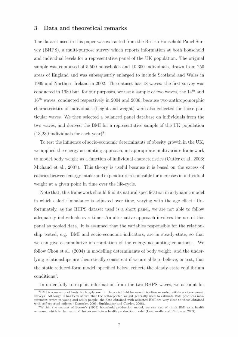
of the sample. In Figure 3 is shown the path of food prices with respect to the

aggregate price index: changes in relative food prices have decreased constantly

each year by 1%, making food (calorie) consumption potentially more convenient.

This is in line with the findings of Lakdawalla and Philipson (2009) in the United

States who, while reporting a reduction in the price of food, also noted that the

market demand for food did not seem to increase4. However, the determinants of

obesity may not affect individuals equally.

This argumentation is partly supported by addictive behaviour in gaining calo-

ries, which, summarises the effects of different (hidden) individual determinant be-

haviours (Cawley, 1999). That is, overweight individuals may ‘’feed on themselves”,

so as obesity issues tend to become more entrenched in already obese individuals5.

This implies that an increase in the relative demand for food by overweight people,

but not necessarily an increase in aggregate food demand, may explain why obesity

is increasing.

As will be argued below, if we rely on the energy accounting framework, in which

2These estimates are discussed in the report ”Tackling Obesities: Future Choices”, 2007.3Bleich et al. (2007) and Pieroni et al. (2010), respectively.4Using historical data Costa and Steckel (1997) show frequently coinciding declines in calories and prices, and

growth in weight. For example, the increasingly larger portions at fastfood outlets and restaurants should also beinterpreted as responses to the growing food supply and consistent with the prediction of falling relative food prices.

5Blanchflower et al. (2009) provide cross-sectional evidence for Germany that overweight perceptions and dietingare influenced by a person’s relative BMI.

4

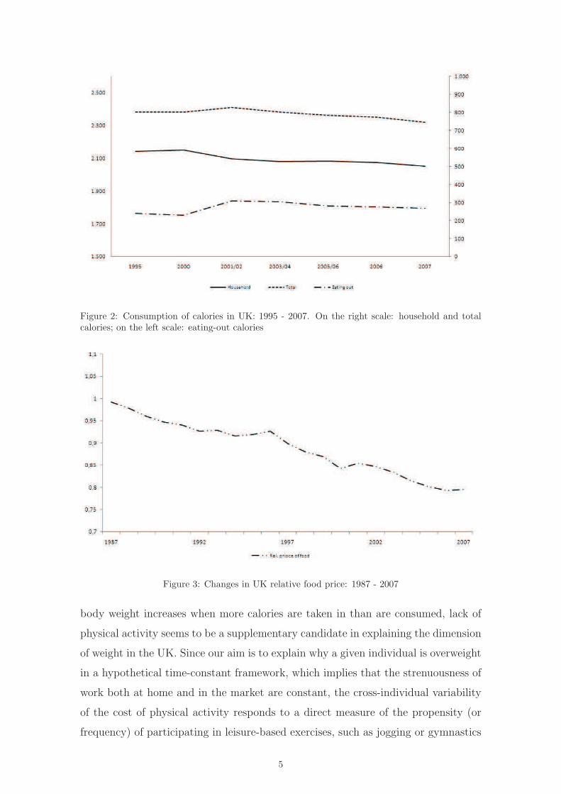
Figure 2: Consumption of calories in UK: 1995 - 2007. On the right scale: household and totalcalories; on the left scale: eating-out calories

Figure 3: Changes in UK relative food price: 1987 - 2007

body weight increases when more calories are taken in than are consumed, lack of

physical activity seems to be a supplementary candidate in explaining the dimension

of weight in the UK. Since our aim is to explain why a given individual is overweight

in a hypothetical time-constant framework, which implies that the strenuousness of

work both at home and in the market are constant, the cross-individual variability

of the cost of physical activity responds to a direct measure of the propensity (or

frequency) of participating in leisure-based exercises, such as jogging or gymnastics

5

or, more in general, of substituting extra hours of work with an increase in physical

exercise.

If we look at the UK, the percentages of both men and women undertaking

physical exercise has increased constantly and considerably over the last ten years6,

but even in 2007, one-third of the population had not kept up with the Government

guidelines for physical exercise. Also in this context, the different roles played by

men and women in the family and society seems to be a constraint for physical

exercise and to affect gender body weight non-equally. The main reasons for not

taking exercise, as they emerged from the survey, were work commitments and lack

of leisure time for men, and exactly the opposite for women (NHS, 2009).

Another explanation for increasing body weight was given by Chou et al. (2004),

who argued that it was the result of several economic changes which have modi-

fied people’s lifestyle choices. In particular, the main changes proposed to affect

weight are: i) changes in relative prices, favouring meals in fast-food and full-service

restaurants, had important effects on overweight; ii) the increasing female work

participation rate, which has reduced the amount of time spent on housework and

cooking meals with basic ingredients, has determined growing weight, even when

the relative prices of eating at home have declined. This theoretical framework as-

sumed that traditional meals are less dense in calories, and that the demand for

convenience foods and unhealthy fast food was a response to the increasing value of

women’s household time; iii) increases in the relative price of cigarettes - as well as

the effects of legislation (clean indoor air laws), which have reduced smoking - may

have contributed to increasing average weight, because smokers may have higher

metabolic rates than non-smokers7.

However, although it could be argued that the rising cost of time based on female

labour force participation and the link with food prices and weight may not be a

current viable option when measured in terms of time correlations (Goldin and

Katz, 2002), there are fundamental reasons (see later) for expecting body fat to be

sensitive to these socio-economic circumstances in the UK. We will return to this

discussion by presenting an identifying extension of body weight determinants in a

more general, although static, framework than that of Chou et al. (2004).

6From 32% in 1997 to 40% in 2007 for men and from 17% to 21% for women.7In the medical literature (Grunberg, 1985; Klesges et al., 1989; French and Jeffery, 1995), changes in dietary

intake, physical activity and metabolic rate are some of the proposed mechanism through which body weight isaffected by smoking.

6

3 Data and theoretical remarks

The dataset used in this paper was extracted from the British Household Panel Sur-

vey (BHPS), a multi-purpose survey which reports information at both household

and individual levels for a representative panel of the UK population. The original

sample was composed of 5,500 households and 10,300 individuals, drawn from 250

areas of England and was subsequently enlarged to include Scotland and Wales in

1999 and Northern Ireland in 2002. The dataset has 18 waves: the first survey was

conducted in 1980 but, for our purposes, we use a sample of two waves, the 14th and

16th waves, conducted respectively in 2004 and 2006, because two anthropomorphic

characteristics of individuals (height and weight) were also collected for those par-

ticular waves. We then selected a balanced panel database on individuals from the

two waves, and derived the BMI for a representative sample of the UK population

(13,230 individuals for each year)8.

To test the influence of socio-economic determinants of obesity growth in the UK,

we applied the energy accounting approach, an appropriate multivariate framework

to model body weight as a function of individual characteristics (Cutler et al. 2003;

Michaud et al., 2007). This theory is useful because it is based on the excess of

calories between energy intake and expenditure responsible for increases in individual

weight at a given point in time over the life-cycle.

Note that, this framework should find its natural specification in a dynamic model

in which calorie imbalance is adjusted over time, varying with the age effect. Un-

fortunately, as the BHPS dataset used is a short panel, we are not able to follow

adequately individuals over time. An alternative approach involves the use of this

panel as pooled data. It is assumed that the variables responsible for the relation-

ship tested, e.g. BMI and socio-economic indicators, are in steady-state, so that

we can give a cumulative interpretation of the energy-accounting equations . We

follow Chou et al. (2004) in modelling determinants of body weight, and the under-

lying relationships are theoretically consistent if we are able to believe, or test, that

the static reduced-form model, specified below, reflects the steady-state equilibrium

conditions9.

In order fully to exploit information from the two BHPS waves, we account for

8BMI is a measure of body fat largely used in the social field because it is often recorded within socio-economicsurveys. Although it has been shown that the self-reported weight generally used to estimate BMI produces mea-surement errors in young and adult people, the data obtained with adjusted BMI are very close to those obtainedwith self-reported indexes (Zagorsky, 2005; Burkhauser and Cawley, 2006).

9Within the context of Becker’s (1965) household production model, we can also of think BMI as a healthoutcome, which is the result of choices made in a health production model (Lakdawalla and Philipson, 2009).

7

short cyclical effects on variables by including a time dummy variable. Its inclusions

is useful in identifying the unobserved time heterogeneity of individuals born in

different periods. This implies that the error terms from both periods are constants

and have the usual assumption for the estimates.

There should be another source of misspecification linked with the steady state

BMI’s respondents. This issue is associated with the heterogeneous responses of in-

dividuals on health behaviours, and in particular, on the choice of the optimal weight

over the life-cycle to the long-term imbalances in energy intake and expenditure. By

including the age variable (or its polynomial specification) in a reduced form of the

model, we could therefore be able to control for the body weight response of a spe-

cific age but anyone ensures that this behaviour will be stable for some time except

for older people that are known to be unaffected by past and current shocks. These

effects - if empirically important - may affect the error structure of the reduced-form

model10.

A relevant sensitivity analysis to verify the equilibrium assumption for our data

is, therefore, to compare the estimated parameters of the benchmark model with

those obtained from a sub-sample which is assumed to be less age-sensitive. The

cumulative interpretation of the energy-accounting equations is consistent with the

view that body weight has stabilized in the older population examined (e.g. in those

over 50). If negligible differences are found between BMI estimates obtained from

the full sample and those from older people, then this should mean that the results

of the complete sample have a high degree of external validity in explaining the

determinants of obesity in the UK.

4 The empirical model

Chou et al. (2004) list a number of hypotheses which link socio-economic determi-

nants to body weight. Referring to their discussion and the literature they cite, we

postulate that the following equation holds:

BMIi,j = f (Si,j, Zj , Di,j , Rj) (1)

where Si,j denotes individual-level influences on body weight, Zj the influences of

regional variables, Di,j is a vector of socio-economic and demographic variables which

10As a by-product, the age variable can correct biases in self-reported measures of BMI, which tends to increasewith age, particularly for height (Burkhauser and Cawley, 2006).

8

control for body weight, and Rj the influence of specific macro-regional variables.

The vector of individual variables Si,j contains as covariates the number of

cigarettes smoked per day and whether or not the mother works. Although an

inverse relationship between smoking and body weight has been documented in the

clinical and economic literature, the effect of cigarette smoking on obesity remains

inconclusive. Focusing on the economic literature, Chou et al. (2004), Rashad and

Grossman (2004) and Baum (2009) have found that the decline in smoking rate by

higher taxes or prices are associated with higher rates of obesity. Consistent with

this finding, Flegal (2007) suggests that a decline in smoking increases obesity but

these effects are estimated to be small. In contrast, Gruber and Frakes (2006) have

found an opposite effect of smoking taxes on obesity using the same data. The evi-

dence of this unexpected relationship was further supported by Cawley et al. (2004)

when females groups were investigated. In addition, Nonnemaker et al. (2009) found

no evidence between higher smoking taxes and obesity rates. With respect to this

literature, the use of the observed consumption, instead of cigarette taxes or prices

in assessing directly its effect on individual weight, may avoid issues associated with

endogeneity. As discussed by Gruber and Frakes (2006), cigarette prices or taxes

are generally recorded at regional or state level, so changes may also be driven by

other market factors which affect both the rates of smoking and eating.

It has been widely argued that increased body weight is a response to expanded

labour market opportunities for women which, by increasing the value of household

time, have also increased the demand for prepared food. Although several studies

have rejected this hypothesis (Cutler et al, 2003; Loureiro and Nayga, 2004), changes

in the relative prices of prepared meals under increasing demand may indirectly

be responsible for increased body weight. Consumption of meals cooked at home

requires time to be spent on them, although there is a positive externality effect

obtained by eating less energy-dense food. Hence, the full price of a meal at home

should reflect the value of the time used to cook it, as well as the monetary price of

the food eaten. Under the hypothesis that, in a post-modern society, the ‘’shadow”

marginal cost of an hour spent cooking at home is greater than the opportunity cost

of an hour at work, the demand for prepared food increases as women, particularly

mothers, tend to participate in work. Thus, average body weight is expected to

increase as the female work participation rate rises.

In his economic analysis of obesity, Philipson (2001) also emphasises the role

9

of innovations which economise on time previously allocated to the non-market

sector. One such innovation, largely tested as a determinant in the obesity literature,

concerns the growing availability of fast food and full-service restaurants. The spread

of fast food is linked with an increase in less expensive food because, the greater

food supply reduces the price of fast food with respect to other foods. In addition,

the content of this food, more energy-dense, may corroborate the hypothesis of

increases in body weight (Schlosser, 2001; Drewnowski, 2003). With respect to

Auld and Powell (2009) and Chou et al. (2004), our data do not use separately

the prices of fast food at UK regional level to test the hypothesis that reductions

in fast-food restaurant prices induce a substitution towards food consumption with

higher calories. In the same way, we maintain the argument by including an index

measuring the price of fruit and vegetables at regional level as a proxy behaviour

of less energy-dense food, i.e. more healthy food, so that we can examine whether

price increases have significant effects on BMI growth. In these and all subsequent

models, we also include the regional price of take-away meals and snacks as a control

variable in Zj. Meeting household needs and work constraints, the great increase

in take-away meals (and snacks) in the UK may have increased the proportion

of energy-dense food in the diet and, on average, overweight. As argued in this

literature, we are interested in testing this hypothesis in women11.

In addition, the level of overweight has been found to be linked with the great

increase in the per capita number of restaurants and fast-food outlets (see also

Rashad et al., 2006). It is known from studies in the United States that such outlets

are located in areas where consumers put a relatively high price on their time. But

this evidence seems to be also confirmed in specific groups of society and by gender.

Currie et al. (2010) have found that, among pregnant women, the residence distance

from fast food restaurants reduce the probability of gaining weight over 20 Kg. In

our empirical analysis, we include the density of restaurant food supply, assumed to

be positively correlated with the higher marginal cost of time for lunch or breaks

while the likely non-linear influence in increasing body weight is captured by the

square of the same variable.

Table 1 lists all demographic variables Di,j as well as the variables included in

the estimates. BMI is assumed to depend on (non-linear) age, race, marital status,

11The literature on food energy density did not confirm the concept that a decrease in the price of energy-densefood tends to increase total calorie consumption at aggregate level: if energy-dense foods become relatively cheaper,we may observe offsetting decreases in the consumption of less dense foods, so that total calories would change oreven decrease (Auld and Powell, 2009).

10

education, and income. Because this weight indicator is essentially used to measure

obesity, individuals of a certain age, income or education may be at higher risk of

being overweight. Schroeter et al. (2008) found that income changes in cross-country

analyses could lead to weight gains, except in cases when all foods were inferior

goods. However, the relationship between within-country income and weight may

differ given the narrow and small cross-country variability of strenuousness level at

work. As argued by Lakdawalla and Philipson (2009), increases in income raise

weight in underweight people, but further increases may actually reduce weight in

obese people. This mechanism is based on the optimal individual BMI which, in

our specification, produces a positive marginal utility of BMI (BMI>0) if changes in

income affect underweight people, and negative (BMI<0) if they affect overweight

people. An inverted U-shaped relationship between income and weight thus emerges.

However, the magnitude of the income effect may be overestimated, due to reverse

causality from obesity to income, i.e., endogeneity. Higher body weight may, indeed,

lead to lower wages, due to effects on productivity or employment discrimination

(Cawley, 2004). Weight and income may also be negatively correlated because of

unobservable personal characteristics, such as self-discipline or impulsivity (Cutler

et al., 2003).

It is clear that densities of food supply and food prices are generally identified by

variations due to supply, rather than demand side-shocks. In our specification, we

reduce the dependence of prices and densities of food supply on demand side-shocks

at regional level by comprising three regional dummy variables, including the effect

of living in London, Yorkshire and the Humber and Scotland. These three regions

are peculiar because, according to ‘’Statistics on Obesity, Physical Activity and

Diet: England, February 2009”, published by the NHS, and ‘’Obesity in Scotland:

an epidemiology briefing”, by the Scottish Public Health Observatory, inner and

outer London are the areas with the lowest levels of obesity in the UK, while those

of Yorkshire and the Humber and Scotland are the highest. In Scotland this result is

true, especially for older women. However, excluding the possibility that the specific

regional variables which we consider are correlated with genetic determinants, we

examine therefore the socio-economic determinants of obesity in the UK net of the

fact that regression disturbance terms may affect estimates.

In the following, we complement an empirical hypothesis with the suggestions of

Lakdawalla and Philipson (2009) to explain why a given individual may be over-

11

Table 1: Data definitions and sources

Variable Definition Source

Job hours Number of hours normally worked per week, BHPS

including overtime

Phys Activity Dummy variable equal to one if respondents make BHPS

physical activity at least once a week

Strenuousness Dummy variable that measures the strenousness of work in which BHPS

respondents’ are involved

PriceF&V Price of fruits and vegetables ONS

PriceTA Price of take away and snacks ONS

Rest/FF Density of restaurants and fast food ONS

Rest/FF2 Squared density of and restaurants and fast food ONS

N Cigarettes Number of cigarettes usually smoked per day BHPS

Work Mother Dummy equal to one if the respondents’ household mother BHPS

is involved in a full time job

Black Dummy equal to one if respondents’ ethnicity is black BHPS

Age Respondents’ age BHPS

Age2 Respondents’ squared age BHPS

Net Income Net household income BHPS

Net Income2 Squared net household income BHPS

Couple Dummy equal to one if respondents’ marital status is couple BHPS

Married Dummy equal to one if respondents’ marital status is married BHPS

Divorced Dummy equal to one if respondents’ marital status is divorced BHPS

Separated Dummy equal to one if respondents’ marital status is separated BHPS

Widowed Dummy equal to one if respondents’ marital status is widowed BHPS

Degree Dummy equal to one if respondents’ education is degree BHPS

Diploma Dummy equal to one if respondents’ education is diploma BHPS

Alevel Dummy equal to one if respondents’ education is Alevel BHPS

Olevel Dummy equal to one if respondents’ education is Olevel BHPS

Note: Data retrieved from British Household Panel Survey (BHPS) and Office for National Statistics (ONS)

weight. We assume that workers who spend more extra hours at their jobs are more

likely to be overweight than those who do normal job hours, because they have

less leisure to devote to leisure activities which, on average, are more physically

demanding. This hypothesis is largely explained by the increases in sedentary job

in post-modern society.

As a strenuous job is assumed to be weak and constant in developed countries and

within specific jobs, we specify and estimate a model that includes as explanatory

variable the number of hours normally worked per week (including overtime) and

12

evaluate whether it causes a rise in body weight.

In Section 2, we showed that the main reasons for not exercising were not only

given as extra work commitments, but also as a lack of leisure time, and that the

latter was mainly suggested by women. We directly proxy physical activity by a

dummy which takes value 1 when an individual exercises at least once a week and

0 otherwise, and verify the heterogeneous influence on body weight by estimating

separate gender models. The (negative) dimension of the estimated coefficient of

individual physical activity on weight indicates how the cost of physical activity

rises. Formally, these specifications are given as:

BMIi,j,k = f (Wi,j,k, Ti,j,k, Dj,k, Rj,k) (1)

where Wi,j,k is a partitioned vector which contains the number of hours worked in

a normal week (including overtime) and the frequency of physical activity; k = 1, 2

are the equations for these separate indicators. Ti,j,k is a dummy variable that

assumes value 1 if the type of work is physically demanding, and Di,k and Ri,k are

vectors of already described variables. Lastly, in view of the heterogeneous gender

behaviour shown above, we also estimate the influence of these equations by gender.

In order to obtain a proper reduced form, we include equation (1) in (2). Thus,

BMIi,j,k = f(Wi,j,k, Ti,j,k, Dj,k, Rj,k

)(2)

where Wi,j,k also includes Si,j,k and Zj,k for the k = 1, 2 equations in vector Wi,j,k,

the vector of variables in (1). In the next section, we explain the use of a quantile

regression framework to allow for the different effect of the same covariate at the

lower tail of BMI individual distribution (underweight) and the upper one (obese).

5 Preliminary results and methods

Figure 4 shows the estimates of Epanechnikov kernel density functions for BMI

distribution conditional on some covariate distributions below and above the median

of our sample, and by gender. As a first result, we examine whether the underlying

assumption for error terms of OLS regression is normally distributed in the covariates

of interest.

Although the empirical conditional distributions for any panel in the figures are

not very far from Gaussian distributions, they do not appear to meet the theoretical

13

0.0

5.1

Kern

el D

ensity E

stim

ate

15 20 25 30 35 40bmi

High price of fruits and vegetables

Low price of fruits and vegetables

kernel = epanechnikov, bandwidth = .84

Male

0.0

2.0

4.0

6.0

8.1

Kern

el D

ensity E

stim

ate

15 20 25 30 35 40bmi

High price of fruits and vegetables

Low price of fruits and vegetables

kernel = epanechnikov, bandwidth = .93

Female

0.0

2.0

4.0

6.0

8.1

Kern

el D

ensity E

stim

ate

15 20 25 30 35 40bmi

High number of job hours

Low number of job hours

kernel = epanechnikov, bandwidth = .61

Male

0.0

2.0

4.0

6.0

8.1

Kern

el D

ensity E

stim

ate

15 20 25 30 35 40bmi

High number of job hours

Low number of job hours

kernel = epanechnikov, bandwidth = .72

Female

0.0

5.1

Kern

el D

ensity E

stim

ate

15 20 25 30 35 40bmi

Physical activity never

Physical activity at least once a week

kernel = epanechnikov, bandwidth = .86

Male

0.0

2.0

4.0

6.0

8.1

Kern

el D

ensity E

stim

ate

15 20 25 30 35 40bmi

Physical activity never

Physical activity at least once a week

kernel = epanechnikov, bandwidth = .93

Female

0.0

2.0

4.0

6.0

8.1

Kern

el D

ensity E

stim

ate

15 20 25 30 35 40bmi

High density of Rest./FF

Low density of Rest./FF

kernel = epanechnikov, bandwidth = .77

Male

0.0

2.0

4.0

6.0

8.1

Kern

el D

ensity E

stim

ate

15 20 25 30 35 40bmi

High density of Rest./FF

Low density of Rest./FF

kernel = epanechnikov, bandwidth = .86

Female

0.0

2.0

4.0

6.0

8.1

Kern

el D

ensity E

stim

ate

15 20 25 30 35 40bmi

Non−smokers

Heavy smokers

kernel = epanechnikov, bandwidth = .55

Male

0.0

2.0

4.0

6.0

8.1

Kern

el D

ensity E

stim

ate

15 20 25 30 35 40bmi

Non−smokers

Heavy smokers

kernel = epanechnikov, bandwidth = .65

Female

Figure 4: Kernel density estimates of BMI by gender

features required by BMI distributions and are skewed.

Table 2 characterises these kernel density estimates of conditional distributions

for BMI means and medians and measures the share of obese people at the threshold

14

(i.e., BMI ≥ 30). For the price of fruit and vegetables, note that the mean for men

living in an area with high prices is 1.59% higher than for those living in an area with

lower prices. The situation is similar for women or when the median is taken into

account. In line with our expectations, the proportion of obese people is estimated

to be 17% of the distribution with respect to people living in areas with higher-priced

fruit and vegetables, and 14% for lower-priced ones, respectively.

Table 2: Means and medians of BMI and share of obese people according to different values oftesting variables

Male Female Total Male Female Total

Variable Mean Median Mean Median Mean Median BMI ≥ 30 BMI ≥ 30 BMI ≥ 30

High price of fruits & vegetables 26.41 26.15 25.54 24.85 25.93 25.54 17.51 16.94 17.27

Low price of fruits & vegetables 25.99 25.63 25.32 24.79 25.64 25.17 14.34 16.52 15.49

High number of job hours 26.42 26.11 25.46 24.62 26.02 25.54 17.38 16.19 16.88

Low number of job hours 26.02 25.63 25.61 24.94 25.76 25.23 15.72 13.69 14.73

Physical activity at least once a week 25.99 25.63 25.16 24.47 25.56 25.11 14.49 14.2 14.34

Physical activity never 26.85 26.52 26.63 26.17 26.72 26.31 22.19 24.98 23.84

High density of Restaurants and fast food 26.61 26.35 25.71 25.16 26.11 25.63 18.86 17.42 18.06

Low density of Restaurants and fast food 26.07 25.68 25.14 24.29 25.57 25.03 17.39 15.14 16.19

High number of cigarettes 25.79 26.11 25.65 25.04 25.73 25.61 17.65 17.83 17.75

Low number of cigarettes 26.46 25.38 25.73 24.85 26.07 25.12 15.08 19.89 17.41

Notes: The share of obese people has been obtained as 1 − F (BMI < 30), where the probability of BMI lower thanthe obesity threshold has been calculated from the cumulative kernel density function of BMI conditioned to testingvariables.

Men working more than 30 hours a week (part-time work threshold) are more

likely to have an average BMI higher than those working 30 hours or less (1.51% and

1.84% for the median). Instead, women do not reveal strong differences in the means

and medians of empirical distributions. If we look at the share of obese adults, it

is easy to note the fall (about 2%) for both men and women working less than 30

hours.

When we look at the variable which records physical activity habits, we observe

huge differences between the BMI means and medians of people exercising at least

once a week and those who never take any physical exercise: 3.31% for the mean

and 3.47% for the median of men and 5.84% for the mean and 6.95% for the median

of women. The quota of estimated obese people for both men and women, is the 8%

higher in the case of nophysical exercise, and this result is largely consistent with

our expectations.

Lower densities of restaurants and fast-food outlets are associated with decreased

BMI means and medians in people resident in such areas. However, the magnitude

of the effects on BMI of the density of restaurants is not as large as expected. Con-

sistently, the shares of obese people living in areas with lower densities of restaurants

and fast-food shops decrease by 1% and 2% for men and women, respectively.

In order to understand the different impact of cigarette consumption on BMI,

15

we functionally split our sample between ”non-smokers”, and ”heavy smokers”12

adults. Kernel densities, plotted by gender, show that the mean and median BMI of

”heavy smokers” are smaller than those of ”non-smokers”. Moreover, the percentage

of obese ”heavy smokers” is smaller than that of obese ”non-smokers”, for men,

although this relation is not supported by the graph for women. Although based on

a descriptive approach, the impact of cigarette consumption seems to be significant

on underweight and normal weight women, progressively falling in influence when

we consider overweight and obese women.

As BMI distributions vary according to the values of the explanatory variables, we

propose a quantile regression approach to estimate the relationship between socio-

economic determinants and BMI. The main empirical advantage is that the flexibility

in estimating parameters at different distribution quantiles does not require any

assumptions regarding error term distribution (Koenker and Bassett, 1978; Koenker

and Hallock, 2001). In addition, some proxies for the socio-economic determinants

which potentially affect body weight are obtained at regional level. The use of

quantile regressions at least avoids including the hypothesis that individuals living

in the same region are subject to similar macro-economic shocks, because there is

no reason to expect that changes in BMI would be equal across individuals.

With this technique, we can carefully examine the determinants of BMI through-

out the conditional distribution, with particular focus on people with the highest

and lowest BMI levels, which are arguably of the greatest interest. We follow the

quantile regression formulation developed by Koenker and Bassett (1978), which

yields parameter estimates at multiple points in the conditional distribution of the

dependent variable13. One particular regression quantile is the solution to

minβ∈RK

∑

i∈{BMIi≥x′β}

θ∣∣∣BMIi − x

′

β∣∣∣+

∑

i∈{BMIi≤x′β}

(1− θ)∣∣∣BMIi − x

′

β∣∣∣

(3)

where θ ∈ (0, 1). The estimates are obtained by minimising the weighted sum

of absolute deviations, obtaining the nth quantile by appropriately weighting the

residuals. The conditional quantile of BMIi, given the vector of explanatory x, is

QBMI (θ|x) = x′

βθ (4)

12”Heavy smokers” are adults smoking more than 20 cigarettes per day.13A helpful introduction to quantile regression appears in Koenker and Hallock (2001). Applications of this

method are increasingly common see for example Hartog et al (2001) and Gorg and Strobl (2002).

16

This formulation is analogous to OLS, E(BMI|x) = x′

β, although OLS slope

parameters are estimated only at the mean of the conditional distribution of the

dependent variable. In summary, the model in equation (5) explains BMI as the

vector of the covariates, with the inclusion of a year dummy variable to remove the

short trends in weight outcomes and covariates and to what extent parameters βθ

change as we move across quantiles. We can then calculate the elasticities to analyse

the policy implications of socio-economic determinants on body weight from the

parameter estimates for each model.

6 Estimates and discussion

Table 3 lists the values of the test of equality across quantiles for the covariates

included in equation (5), separately for the equation which includes job hours (here-

after, model (1)) and physical activities (model (2)). This test is valid if, at least,

one estimated percentile coefficient has a different effect with respect to the others.

For the equations for women, we find larger differences in quantile estimates (e.g.,

physical activity habits, strenuousness of job, price of fruit and vegetables, density of

restaurants and fast-food shops and its square, number of cigarettes smoked, black

ethnicity, net income and net income squared, age and age squared, marital status,

and education). For men, these differences in covariates are less marked (effects are

significant for: physical activity habits, age and age squared, marital status and

education). Thus, we proceed to estimate models by quantile regressions, and use

OLS estimates to compare results.

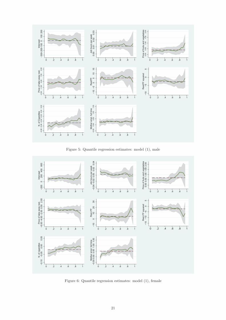
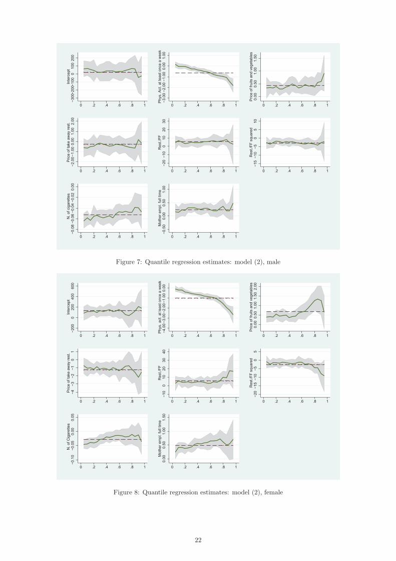
Tables 4 and 5 list the BMI estimates of models (1) and (2) for selected quantiles

between the 10th and 90th of the distribution. The parameter estimates of quantile

regressions by gender are also shown in Figures 5-814.

Irrespective of the model used, the estimated parameters of the (socio-demographic)

control covariates are generally of the expected signs. Black respondents have a

higher BMI than white respondents and, mostly for women, the coefficients vary

across quantiles. Higher education is associated with a lower BMI. In addition, in-

come effects are not significant for UK male respondents but are negative for female

ones, for both OLS and quantile regressions after the median of the BMI distribu-

14We report the empirical BMI distribution which corresponds to some points of quantile estimates. The 10th

percentile of BMI distribution corresponds to a BMI of 20.65 Kg/m2 for men and 20.72 Kg/m2 for women, the25th to 22.62 Kg/m2 for men and 23 Kg/m2 for women, the 50th to 25.23 Kg/m2 for men and 25.62 Kg/m2 forwomen, the 75th to 28.48 Kg/m2 for men and 28.81 for women, and the 90th to 31.95 Kg/m2 for men and 32.50Kg/m2 for women.

17

Table 3: Test for equality of coefficients across quantiles

Models

(1) (2)

Variable M F M F

Job hours 0.28 1.54 - -

(0.889) (0.188) - -

Phys Act - - 28.59 17.28

- - (0.000) (0.000)

Strenuousness 1.74 1.48 1.91 2.04

(0.138) (0.204) (0.107) (0.086)

PriceF&V 0.45 1.95 0.51 2.46

(0.774) (0.099) (0.729) (0.043)

PriceTA 0.22 0.69 0.61 0.83

(0.924) (0.597) (0.663) (0.507)

Rest/FF 0.94 3.26 0.81 1.71

(0.442) (0.011) (0.517) (0.145)

Rest/FF2 1.07 3.87 1.01 2.79

(0.369) (0.004) (0.411) (0.024)

N Cigarettes 1.28 5.61 0.61 4.75

(0.275) (0.002) (0.662) (0.000)

Work Mother 0.29 2.14 0.82 1.07

(0.886) (0.073) (0.513) (0.369)

Black 1.04 3.47 0.18 2.71

(0.384) (0.007) (0.951) (0.029)

Age 12.17 21.03 12.34 11.93

(0.000) (0.000) (0.000) (0.000)

Age2 14.37 18.72 17.38 12.41

(0.000) (0.000) (0.000) (0.000)

Net Income 0.65 4.06 0.36 3.88

(0.627) (0.002) (0.839) (0.003)

Net Income2 0.03 2.41 0.28 2.49

(0.999) (0.047) (0.888) (0.041)

Couple 0.65 0.591 1.01 0.23

(0.627) (0.672) (0.408) (0.922)

Married 2.42 0.91 1.82 0.28

(0.046) (0.463) (0.125) (0.891)

Divorced 1.84 3.14 3.18 3.53

(0.118) (0.014) (0.012) (0.007)

Separated 1‘.14 1.11 1.22 1.23

(0.335) (0.355) (0.301) (0.296)

Widowed 2.27 2.8 3.27 1.06

(0.059) (0.024) (0.010) (0.376)

Degree 3.81 4.55 7.66 3.81

(0.004) (0.001) (0.000) (0.007)

Diploma 3.95 7.51 4.19 1.91

(0.003) (0.000) (0.002) (0.105)

Alevel 4.09 2.05 7.68 2.03

(0.002) (0.085) (0.000) (0.087)

Olevel 8.64 1.82 8.59 3.53

(0.000) (0.122) (0.000) (0.007)

Note: p-values are shown in brackets and significant levels are reportedwith the following notation:Model (1) includes in the vector of the explanatory variables job hourswhile model (2) uses physical activity.

tion, but with very different effects. Married respondents have a BMI similar to

that of couples, but greater than divorced, separated or widowed people.

18

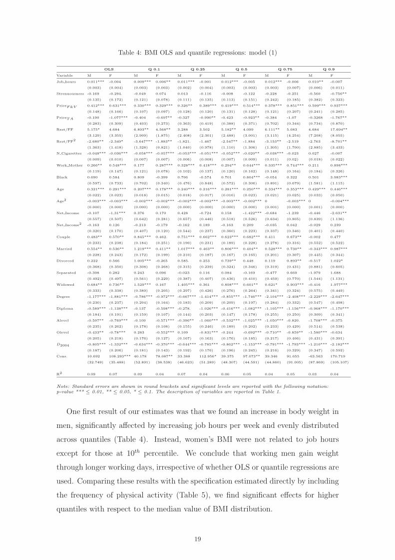
Table 4: BMI OLS and quantile regressions: model (1)

OLS Q 0.1 Q 0.25 Q 0.5 Q 0.75 Q 0.9

Variable M F M F M F M F M F M F

Job hours 0.011*** -0.004 0.009*** 0.006** 0.011*** -0.001 0.012*** -0.005 0.012*** -0.006 0.010** -0.007

(0.003) (0.004) (0.003) (0.003) (0.002) (0.004) (0.003) (0.003) (0.003) (0.007) (0.006) (0.011)

Strenuousness -0.169 -0.294. -0.049 0.074 0.013 -0.116 -0.008 -0.122 -0.228 -0.251 -0.560 -0.756**

(0.135) (0.172) (0.121) (0.078) (0.111) (0.135) (0.113) (0.151) (0.242) (0.185) (0.382) (0.323)

PriceF&V 0.412*** 0.631*** 0.330*** 0.329*** 0.326** 0.389*** 0.419*** 0.514*** 0.378*** 0.851*** 0.599*** 0.937***

(0.148) (0.166) (0.107) (0.097) (0.128) (0.120) (0.131) (0.128) (0.121) (0.207) (0.241) (0.285)

PriceTA -0.190 -1.077*** -0.404 -0.697** -0.327 -0.990** -0.423 -0.923** -0.384 -1.07 -0.3268 -1.767**

(0.283) (0.309) (0.403) (0.273) (0.363) (0.419) (0.388) (0.371) (0.702) (0.344) (0.734) (0.870)

Rest/FF 5.175* 4.684 6.893** 4.568** 3.288 3.502 5.182** 4.099 6.111** 5.083 4.684 17.694**

(3.129) (3.355) (2.909) (1.875) (2.408) (2.301) (2.488) (3.001) (3.115) (4.254) (7.208) (8.055)

Rest/FF2 -2.680** -2.349* -3.647*** -1.883** -1.821. -1.467 -2.547** -1.884 -3.153** -2.519 -2.763 -8.701**

(1.363) (1.418) (1.328) (0.821) (1.040) (0.978) (1.110) (1.306) (1.305) (1.700) (2.885) (3.433)

N Cigarettes -0.048*** -0.036*** -0.058*** -0.057*** -0.053*** -0.051*** -0.052*** -0.020** -0.038*** -0.023 0.027 -0.007

(0.009) (0.010) (0.007) (0.007) (0.006) (0.008) (0.007) (0.009) (0.011) (0.02) (0.018) (0.022)

Work Mother 0.266** 0.548*** 0.177 0.287*** 0.328*** 0.418*** 0.294** 0.644*** 0.335*** 0.744*** 0.211 0.898***

(0.119) (0.147) (0.121) (0.078) (0.102) (0.137) (0.120) (0.162) (0.148) (0.164) (0.184) (0.326)

Black 0.690 0.584 0.809 -0.399 0.706 -0.574 0.701 0.804*** -0.054 0.322 0.501 3.983***

(0.597) (0.733) (0.702) (0.340) (0.476) (0.848) (0.572) (0.306) (0.891) (0.679) (1.581) (1.115)

Age 0.321*** 0.291*** 0.207*** 0.178*** 0.240*** 0.216*** 0.281*** 0.250*** 0.334*** 0.353*** 0.429*** 0.446***

(0.022) (0.023) (0.018) (0.015) (0.018) (0.017) (0.016) (0.023) (0.021) (0.025) (0.033) (0.050)

Age2 -0.003*** -0.003*** -0.002*** -0.002*** -0.002*** -0.002*** -0.003*** -0.002*** 0 -0.003*** 0 -0.004***

(0.000) (0.000) (0.000) (0.000) (0.000) (0.000) (0.000) (0.000) (0.001) (0.000) (0.001) (0.000)

Net Income -0.107 -1.31*** 0.376 0.170 0.428 -0.724 0.158 -1.422*** -0.684 -1.239 -0.446 -2.631**

(0.557) (0.507) (0.642) (0.281) (0.657) (0.446) (0.518) (0.526) (0.634) (0.805) (0.839) (1.136)

Net Income2 -0.163 0.126 -0.213 -0.179 -0.162 0.189 -0.163 0.209 -0.035 0.042 -0.029 0.239

(0.320) (0.170) (0.407) (0.120) (0.544) (0.237) (0.360) (0.223) (0.337) (0.346) (0.401) (0.440)

Couple 0.483** 0.570** 0.845*** 0.462. 0.751*** 0.662*** 0.623*** 0.682*** 0.411 0.673** -0.002 0.477

(0.233) (0.238) (0.184) (0.251) (0.190) (0.231) (0.189) (0.228) (0.278) (0.316) (0.552) (0.522)

Married 0.554** 0.536** 1.219*** 0.411** 1.017*** 0.463** 0.806*** 0.404** 0.528*** 0.730** -0.343*** 0.987***

(0.228) (0.243) (0.172) (0.199) (0.210) (0.187) (0.167) (0.165) (0.201) (0.307) (0.445) (0.344)

Divorced 0.222 0.566 1.005*** -0.265 0.585. 0.253 0.739** 0.448 0.119 0.893** -0.517 1.022*

(0.368) (0.350) (0.308) (0.268) (0.315) (0.239) (0.324) (0.346) (0.319) (0.431) (0.881) (0.605)

Separated -0.398 0.282 0.243 0.096 -0.023 0.116 0.084 -0.169 -0.477 0.669 -1.979 1.688

(0.492) (0.497) (0.561) (0.229) (0.387) (0.407) (0.436) (0.410) (0.459) (0.770) (1.544) (1.131)

Widowed 0.684** 0.736** 1.529*** 0.167 1.405*** 0.361 0.898*** 0.601** 0.621* 0.903*** -0.416 1.977***

(0.333) (0.338) (0.389) (0.205) (0.297) (0.426) (0.276) (0.264) (0.341) (0.324) (0.575) (0.449)

Degree -1.177*** -1.881*** -0.786*** -0.972*** -0.667*** -1.414*** -0.855*** -1.746*** -2.104*** -2.408*** -2.229*** -2.647***

(0.230) (0.237) (0.204) (0.164) (0.183) (0.209) (0.209) (0.197) (0.284) (0.332) (0.547) (0.498)

Diploma -0.589*** -1.138*** -0.137 -0.598*** -0.278. -1.026*** -0.416*** -1.082*** -1.105*** -1.156*** -0.968*** -1.170***

(0.184) (0.191) (0.159) (0.107) (0.144) (0.203) (0.147) (0.178) (0.255) (0.250) (0.309) (0.341)

Alevel -0.597** -0.769*** -0.100 -0.571*** -0.396** -1.060*** -0.532*** -1.025*** -1.050*** -0.820. -1.708*** -0.375

(0.235) (0.262) (0.178) (0.108) (0.155) (0.246) (0.189) (0.202) (0.233) (0.429) (0.514) (0.538)

Olevel -0.433** -0.78*** 0.283 -0.552*** 0.109 -0.831*** -0.244 -0.692*** -0.710** -0.859** -1.580*** -0.634

(0.205) (0.218) (0.176) (0.127) (0.167) (0.163) (0.176) (0.185) (0.217) (0.406) (0.431) (0.391)

D2004 -0.805*** -1.332*** -0.634*** -0.370*** -0.644*** -0.785*** -0.862*** -1.153*** -0.791*** -1.793*** -1.210*** -2.182***

(0.187) (0.206) (0.181) (0.143) (0.192) (0.176) (0.196) (0.245) (0.216) (0.329) (0.347) (0.592)

Cons. 10.692 108.293*** 40.178 78.087** 33.388 112.956* 39.375 97.073** 39.346 91.655 -63.563 170.719

(32.749) (35.488) (52.891) (38.538) (46.623) (51.289) (48.307) (44.591) (44.860) (91.005) (87.869) (105.107)

R2 0.09 0.07 0.09 0.04 0.07 0.04 0.06 0.05 0.04 0.05 0.03 0.04

Note: Standard errors are shown in round brackets and significant levels are reported with the following notation:p-value *** ≤ 0.01, ** ≤ 0.05, * ≤ 0.1. The description of variables are reported in Table 1.

One first result of our estimates was that we found an increase in body weight in

men, significantly affected by increasing job hours per week and evenly distributed

across quantiles (Table 4). Instead, women’s BMI were not related to job hours

except for those at 10th percentile. We conclude that working men gain weight

through longer working days, irrespective of whether OLS or quantile regressions are

used. Comparing these results with the specification estimated directly by including

the frequency of physical activity (Table 5), we find significant effects for higher

quantiles with respect to the median value of BMI distribution.

19

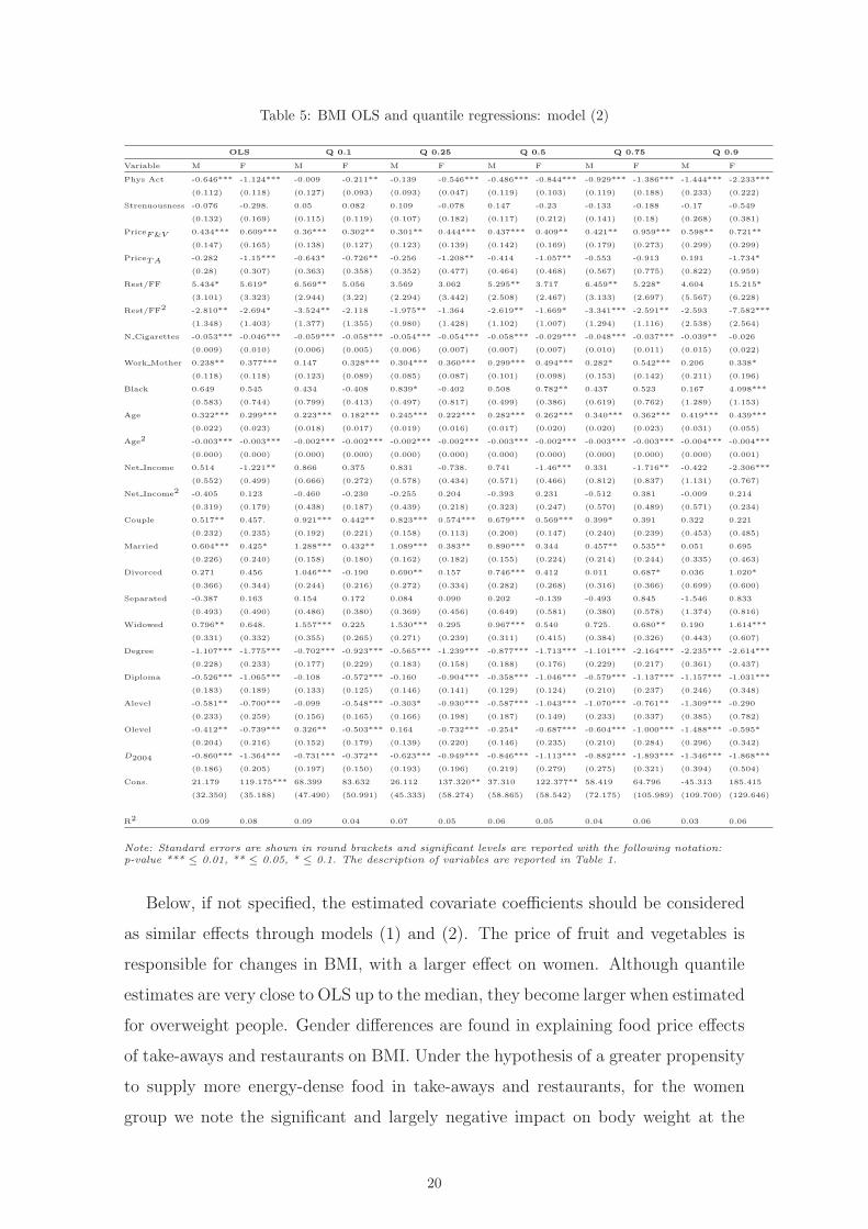
Table 5: BMI OLS and quantile regressions: model (2)

OLS Q 0.1 Q 0.25 Q 0.5 Q 0.75 Q 0.9

Variable M F M F M F M F M F M F

Phys Act -0.646*** -1.124*** -0.009 -0.211** -0.139 -0.546*** -0.486*** -0.844*** -0.929*** -1.386*** -1.444*** -2.233***

(0.112) (0.118) (0.127) (0.093) (0.093) (0.047) (0.119) (0.103) (0.119) (0.188) (0.233) (0.222)

Strenuousness -0.076 -0.298. 0.05 0.082 0.109 -0.078 0.147 -0.23 -0.133 -0.188 -0.17 -0.549

(0.132) (0.169) (0.115) (0.119) (0.107) (0.182) (0.117) (0.212) (0.141) (0.18) (0.268) (0.381)

PriceF&V 0.434*** 0.609*** 0.36*** 0.302** 0.301** 0.444*** 0.437*** 0.409** 0.421** 0.959*** 0.598** 0.721**

(0.147) (0.165) (0.138) (0.127) (0.123) (0.139) (0.142) (0.169) (0.179) (0.273) (0.299) (0.299)

PriceTA -0.282 -1.15*** -0.643* -0.726** -0.256 -1.208** -0.414 -1.057** -0.553 -0.913 0.191 -1.734*

(0.28) (0.307) (0.363) (0.358) (0.352) (0.477) (0.464) (0.468) (0.567) (0.775) (0.822) (0.959)

Rest/FF 5.434* 5.619* 6.569** 5.056 3.569 3.062 5.295** 3.717 6.459** 5.228* 4.604 15.215*

(3.101) (3.323) (2.944) (3.22) (2.294) (3.442) (2.508) (2.467) (3.133) (2.697) (5.567) (6.228)

Rest/FF2 -2.810** -2.694* -3.524** -2.118 -1.975** -1.364 -2.619** -1.669* -3.341*** -2.591** -2.593 -7.582***

(1.348) (1.403) (1.377) (1.355) (0.980) (1.428) (1.102) (1.007) (1.294) (1.116) (2.538) (2.564)

N Cigarettes -0.053*** -0.046*** -0.059*** -0.058*** -0.054*** -0.054*** -0.058*** -0.029*** -0.048*** -0.037*** -0.039** -0.026

(0.009) (0.010) (0.006) (0.005) (0.006) (0.007) (0.007) (0.007) (0.010) (0.011) (0.015) (0.022)

Work Mother 0.238** 0.377*** 0.147 0.328*** 0.304*** 0.360*** 0.299*** 0.494*** 0.282* 0.542*** 0.206 0.338*

(0.118) (0.118) (0.123) (0.089) (0.085) (0.087) (0.101) (0.098) (0.153) (0.142) (0.211) (0.196)

Black 0.649 0.545 0.434 -0.408 0.839* -0.402 0.508 0.782** 0.437 0.523 0.167 4.098***

(0.583) (0.744) (0.799) (0.413) (0.497) (0.817) (0.499) (0.386) (0.619) (0.762) (1.289) (1.153)

Age 0.322*** 0.299*** 0.223*** 0.182*** 0.245*** 0.222*** 0.282*** 0.262*** 0.340*** 0.362*** 0.419*** 0.439***

(0.022) (0.023) (0.018) (0.017) (0.019) (0.016) (0.017) (0.020) (0.020) (0.023) (0.031) (0.055)

Age2 -0.003*** -0.003*** -0.002*** -0.002*** -0.002*** -0.002*** -0.003*** -0.002*** -0.003*** -0.003*** -0.004*** -0.004***

(0.000) (0.000) (0.000) (0.000) (0.000) (0.000) (0.000) (0.000) (0.000) (0.000) (0.000) (0.001)

Net Income 0.514 -1.221** 0.866 0.375 0.831 -0.738. 0.741 -1.46*** 0.331 -1.716** -0.422 -2.306***

(0.552) (0.499) (0.666) (0.272) (0.578) (0.434) (0.571) (0.466) (0.812) (0.837) (1.131) (0.767)

Net Income2 -0.405 0.123 -0.460 -0.230 -0.255 0.204 -0.393 0.231 -0.512 0.381 -0.009 0.214

(0.319) (0.179) (0.438) (0.187) (0.439) (0.218) (0.323) (0.247) (0.570) (0.489) (0.571) (0.234)

Couple 0.517** 0.457. 0.921*** 0.442** 0.823*** 0.574*** 0.679*** 0.569*** 0.399* 0.391 0.322 0.221

(0.232) (0.235) (0.192) (0.221) (0.158) (0.113) (0.200) (0.147) (0.240) (0.239) (0.453) (0.485)

Married 0.604*** 0.425* 1.288*** 0.432** 1.089*** 0.383** 0.890*** 0.344 0.457** 0.535** 0.051 0.695

(0.226) (0.240) (0.158) (0.180) (0.162) (0.182) (0.155) (0.224) (0.214) (0.244) (0.335) (0.463)

Divorced 0.271 0.456 1.046*** -0.190 0.690** 0.157 0.746*** 0.412 0.011 0.687* 0.036 1.020*

(0.366) (0.344) (0.244) (0.216) (0.272) (0.334) (0.282) (0.268) (0.316) (0.366) (0.699) (0.600)

Separated -0.387 0.163 0.154 0.172 0.084 0.090 0.202 -0.139 -0.493 0.845 -1.546 0.833

(0.493) (0.490) (0.486) (0.380) (0.369) (0.456) (0.649) (0.581) (0.380) (0.578) (1.374) (0.816)

Widowed 0.796** 0.648. 1.557*** 0.225 1.530*** 0.295 0.967*** 0.540 0.725. 0.680** 0.190 1.614***

(0.331) (0.332) (0.355) (0.265) (0.271) (0.239) (0.311) (0.415) (0.384) (0.326) (0.443) (0.607)

Degree -1.107*** -1.775*** -0.702*** -0.923*** -0.565*** -1.239*** -0.877*** -1.713*** -1.101*** -2.164*** -2.235*** -2.614***

(0.228) (0.233) (0.177) (0.229) (0.183) (0.158) (0.188) (0.176) (0.229) (0.217) (0.361) (0.437)

Diploma -0.526*** -1.065*** -0.108 -0.572*** -0.160 -0.904*** -0.358*** -1.046*** -0.579*** -1.137*** -1.157*** -1.031***

(0.183) (0.189) (0.133) (0.125) (0.146) (0.141) (0.129) (0.124) (0.210) (0.237) (0.246) (0.348)

Alevel -0.581** -0.700*** -0.099 -0.548*** -0.303* -0.930*** -0.587*** -1.043*** -1.070*** -0.761** -1.309*** -0.290

(0.233) (0.259) (0.156) (0.165) (0.166) (0.198) (0.187) (0.149) (0.233) (0.337) (0.385) (0.782)

Olevel -0.412** -0.739*** 0.326** -0.503*** 0.164 -0.732*** -0.254* -0.687*** -0.604*** -1.000*** -1.488*** -0.595*

(0.204) (0.216) (0.152) (0.179) (0.139) (0.220) (0.146) (0.235) (0.210) (0.284) (0.296) (0.342)

D2004 -0.860*** -1.364*** -0.731*** -0.372** -0.623*** -0.949*** -0.846*** -1.113*** -0.882*** -1.893*** -1.346*** -1.868***

(0.186) (0.205) (0.197) (0.150) (0.193) (0.196) (0.219) (0.279) (0.275) (0.321) (0.394) (0.504)

Cons. 21.179 119.175*** 68.399 83.632 26.112 137.320** 37.310 122.377** 58.419 64.796 -45.313 185.415

(32.350) (35.188) (47.490) (50.991) (45.333) (58.274) (58.865) (58.542) (72.175) (105.989) (109.700) (129.646)

R2 0.09 0.08 0.09 0.04 0.07 0.05 0.06 0.05 0.04 0.06 0.03 0.06

Note: Standard errors are shown in round brackets and significant levels are reported with the following notation:p-value *** ≤ 0.01, ** ≤ 0.05, * ≤ 0.1. The description of variables are reported in Table 1.

Below, if not specified, the estimated covariate coefficients should be considered

as similar effects through models (1) and (2). The price of fruit and vegetables is

responsible for changes in BMI, with a larger effect on women. Although quantile

estimates are very close to OLS up to the median, they become larger when estimated

for overweight people. Gender differences are found in explaining food price effects

of take-aways and restaurants on BMI. Under the hypothesis of a greater propensity

to supply more energy-dense food in take-aways and restaurants, for the women

group we note the significant and largely negative impact on body weight at the

20

−3

00−

20

0−1

00

01

00

20

0In

terc

ep

t

0 .2 .4 .6 .8 1

0.0

00

.01

0.0

20

.03

Jo

b h

ou

rs p

er

we

ek

0 .2 .4 .6 .8 1

0.0

00

.50

1.0

01

.50

2.0

0

Price

of

fru

its a

nd

ve

ge

tab

les

0 .2 .4 .6 .8 1

−2

.00

−1

.00

0.0

01

.00

2.0

0

Price

of

take

aw

ay r

est.

0 .2 .4 .6 .8 1

−1

0−

50

51

01

5R

est/

FF

.

0 .2 .4 .6 .8 1

−1

0−

50

5R

est/

FF

sq

ua

red

0 .2 .4 .6 .8 1

−0

.08

−0

.06

−0

.04

−0

.02

0.0

00

.02

N.

of

Cig

are

tte

s

0 .2 .4 .6 .8 1

−0

.50

0.0

00

.50

1.0

01

.50

Mo

the

r e

mp

l. f

ull

tim

e

0 .2 .4 .6 .8 1

Figure 5: Quantile regression estimates: model (1), male

−2

00

02

00

40

06

00

Inte

rce

pt

0 .2 .4 .6 .8 1

−0

.04

−0

.02

0.0

00

.02

0.0

4Jo

b h

ou

rs p

er

we

ek

0 .2 .4 .6 .8 1

0.0

00

.50

1.0

01

.50

2.0

0P

rice

of

fru

its a

nd

ve

ge

tab

les

0 .2 .4 .6 .8 1

−6

.00

−4

.00

−2

.00

0.0

02

.00

Price

of

take

aw

ay r

est.

0 .2 .4 .6 .8 1

−1

00

10

20

30

Re

st.

/FF

0 .2 .4 .6 .8 1

−1

5−

10

−5

05

Re

st.

/FF

sq

ua

red

0 .2 .4 .6 .8 1

−0

.10

−0

.05

0.0

00

.05

N.

of

cig

are

tte

s

0 .2 .4 .6 .8 1

−0

.50

0.0

00

.50

1.0

01

.50

Mo

the

r e

mp

l. f

ull

tim

e

0 .2 .4 .6 .8 1

Figure 6: Quantile regression estimates: model (1), female

21

−3

00−

20

0−1

00

01

00

20

0In

terc

ep

t

0 .2 .4 .6 .8 1

−3

.00

−2

.00

−1

.00

0.0

01

.00

Ph

ys.

Act.

at

lea

st

on

ce

a w

ee

k

0 .2 .4 .6 .8 1

0.0

00

.50

1.0

01

.50

Price

of

fru

its a

nd

ve

ge

tab

les

0 .2 .4 .6 .8 1

−2

.00

−1

.00

0.0

01

.00

2.0

0P

rice

of

take

aw

ay r

est.

0 .2 .4 .6 .8 1

−2

0−

10

01

02

03

0R

est.

/FF

0 .2 .4 .6 .8 1

−1

5−

10

−5

05

10

Re

st.

/FF

sq

ua

red

0 .2 .4 .6 .8 1

−0

.08

−0

.06

−0

.04

−0

.02

0.0

0N

. o

f cig

are

tte

s

0 .2 .4 .6 .8 1

−0

.50

0.0

00

.50

1.0

0M

oth

er

em

pl. f

ull

tim

e

0 .2 .4 .6 .8 1

Figure 7: Quantile regression estimates: model (2), male

−2

00

02

00

40

06

00

Inte

rce

pt

0 .2 .4 .6 .8 1

−4

.00

−3

.00

−2

.00

−1

.00

0.0

0P

hys.

act.

at

lea

st

on

ce

a w

ee

k

0 .2 .4 .6 .8 1

0.0

00

.50

1.0

01

.50

2.0

0P

rice

of

fru

its a

nd

ve

ge

tab

les

0 .2 .4 .6 .8 1

−4

−3

−2

−1

01

Price

of

take

aw

ay r

est.

0 .2 .4 .6 .8 1

−1

00

10

20

30

40

Re

st.

/FF

0 .2 .4 .6 .8 1

−2

0−

15

−1

0−

50

5R

est.

/FF

sq

ua

red

0 .2 .4 .6 .8 1

−0

.10

−0

.05

0.0

00

.05

N.

of

Cig

are

tte

s

0 .2 .4 .6 .8 1

0.0

00

.50

1.0

01

.50

Mo

the

r e

mp

l. f

ull

tim

e

0 .2 .4 .6 .8 1

Figure 8: Quantile regression estimates: model (2), female

22

90th percentile. The dimension of these effects is also confirmed by including the

presence in the household of a working mother.

The density of full-service and fast-food restaurants is significant for some quan-

tiles of the samples analysed. Their growing availability positively affects men’s

BMI, with positive and significant coefficients in the 10th, 50th and 90th quantiles,

and is barely significant for the OLS model. The coefficient is almost the same across

quantiles, except for the 90th percentile, where its measure is three times larger than

that of OLS. Apart from the 90th quantile parameter, none of the others is significant

for women. These estimates are consistent with the results obtained by Chou et al.

(2004). The density of restaurants and fast-food shops induces an increase in the

BMI in men who spend more time at work while, on average, it is less responsible

for increased BMI in women. This result is contradicted by the estimates at the 90th

quantile, where the values for overweight women become statistically significant.

In line with the explanation for men, the effect of the spread of restaurants and

fast-food outlets on high BMI seems to depend positively on extra time worked,

stimulating a demand for outside food, mainly fast-food, which increases calorie in-

take15. Lastly, also in the UK a negative association between cigarette consumption

and BMI is empirically confirmed, and this is true for each estimated quantile except

the most extreme deciles. Policy-makers should note that the significance of OLS

estimates is due to the contributions up to the 75th percentile, although this effect

on BMI is lower in women (see parameters of Table 5)16.

As discussed in section 3, we estimate quantile regressions for the subsample of

people aged over 50, assumed to be stable to long-term imbalances in energy intake

and expenditure. The results are listed in Appendixes A and B. With respect to the

estimates for the complete sample showed in Table 4 and 5, we do not find remark-

able differences in the coefficients of covariates affecting weight distribution. Only

for several central quantiles, we denote slightly larger difference of the estimated pa-

rameters of age covariate between two samples. This implies that we cannot reject a

BMI’s steady-state condition and consistently estimate the behaviour of UK adults

using the complete sample17.

Table 6 lists the estimated BMI effects of a 1% increase in the covariates de-15Although data are not reported, the dataset does show a positive relationship between extra job hours and

larger share of women’s BMI. This additional analysis is available from the authors upon request.16In the specification of model 1, the contribution to the aggregate impact of cigarettes on BMI is also significant

at the 75th percentile for women.17We also performed estimations that included higher polynomial orders of age covariate. The estimates were

close to those reported in Table 4 and 5 and Appendix A and B, that included the covariate age and age squared.

23

scribed above. As previously stated, health policies based on OLS results would not

efficiently measure their influence on overweight and policy suggestions. For exam-

ple, if we focus on the price of fruit and vegetables, we note low estimated elasticity

from OLS for men and women, but it becomes larger in quantile regressions when

we consider women located beyond the 75th percentile. The Table shows that most

of these effects are quite minor, and often fail to be large or precisely measured

enough to achieve statistical significance. The results thus indicate that changes in

the price of fruit and vegetables affect each quantile of the BMI distribution with

moderate effects for overweight people. Restaurant and fast-food densities have a

significant effect on weight for men and women over the 50th percentile. As expected,

the number of cigarettes has a significant negative effect on body weight for much

of the empirical distribution.

Table 6: BMI effect of a 1% increase of selected variables: model(1)

OLS Q 0.1 Q 0.25 Q 0.5 Q 0.75 Q 0.9

Variable M F M F M F M F M F M F

Job hours (x100) 0.042*** -0.016 0.039*** 0.031* 0.045*** -0.001 0.048*** -0.02 0.041*** -0.022 0.035** -0.022

(0.012) (0.021) (0.011) (0.017) (0.009) (0.017) (0.01) (0.018) (0.012) (0.024) (0.014) (0.034)

PriceF&V 0.016*** 0.024*** 0.015** 0.016*** 0.014*** 0.017*** 0.016*** 0.021*** 0.013*** 0.03*** 0.019*** 0.029***

(0.006) (0.006) (0.006) (0.005) (0.005) (0.006) (0.005) (0.006) (0.005) (0.005) (0.007) (0.011)

PriceTA -0.007 -0.042*** -0.019 -0.034 -0.014 -0.044*** -0.016 -0.037** -0.013 -0.038** 0.01 -0.055

(0.011) (0.012) (0.02) (0.023) (0.012) (0.016) (0.014) (0.015) (0.016) (0.019) (0.026) (0.039)

Rest/FF 0.196* 0.181 0.317** 0.223** 0.14 0.156 0.201*** 0.164 0.214* 0.179* 0.149 0.547***

(0.119) (0.13) (0.154) (0.108) (0.104) (0.101) (0.071) (0.103) (0.119) (0.106) (0.182) (0.196)

N Cigarettes -0.002*** -0.001*** -0.003*** -0.003*** -0.002*** -0.002*** -0.002*** -0.001** -0.001*** -0.001** -0.001* 0.000

(0.000) (0.000) (0.000) (0.000) (0.000) (0.000) (0.000) (0.000) (0.000) (0.000) (0.001) (0.000)

Net Income -0.004 -0.051*** 0.017 0.008 0.018 -0.032** 0.006 -0.057*** -0.024 -0.044* -0.014 -0.081**

(0.021) (0.02) (0.028) (0.015) (0.019) (0.014) (0.021) (0.014) (0.029) (0.025) (0.042) (0.038)

Note: Standard errors are shown in round brackets and significant levels are reported with the following notation:p-value *** ≤ 0.01, ** ≤ 0.05, * ≤ 0.1.

However, these effects may have more intuitive implications when they are ex-

pressed as changes in body weight due to policy interventions. Let us consider a

representative adult at the average of the sample and at the 90th percentile of the

conditional BMI distributions for men and women. Admit a subsidy which decreases

the price of fruit and vegetables and encourages the consumption of these healthier

food. The value of these ‘’thin subsidies” is assumed to be 20% of the market price.

Following our OLS estimates in Table 6 (model 1) carried out by gender, BMI would

decrease by about 0.32% for men and 0.47% for women but would increase to 0.38%

and 0.58%, respectively, when we measure the effects for people at the 90th per-

centile. This means that a man 1.75 m tall, weighting 80.23 kg at the mean of the

sample, corresponding to the average BMI (26.2) could expect to be lighter by 0.26

Kg per year, whereas a representative woman (height 1.61 m and BMI 25.43) could

24

expect a decrease of 0.33 kg if price subsidies for healthy food were available. This

reduction is emphasised when we evaluate people at the 90th percentile. In this case,

the effects of reduced body weight are 0.37 kg for men and 0.51 kg for women. We do

not have a specular proxy for evaluating the effects of taxation on unhealthy foods.

We note that, as an alternative impact on body weight, several countries plan to

impose or broaden sales taxes on soft drinks and other food items (for a discussion,

see Uhlman, 2003). This is in line with several recent laws passed to discourage the

consumption of unhealthy foods by increasing their effective prices to consumers.

The UK has considered the introduction of various value-added taxes for food of

poor nutritional value (Kuchler et al., 2005; Schoreter et al, 2008) although this has

been recognised as a progressive burden for low-income families which spend a large

portion of their income on food (e.g., Cash et al., 2004).

We can repeat the exercise for changes in income. In addition to ‘’fat” taxes and

‘’thin” subsidies, several studies have determined that income has a major influence

on obesity (e.g. Deaton, 2003; Drenowsky, 2003). In developed economies, house-

holds with higher incomes tend to consume higher-quality diets consisting mainly of

low-calorie foods, whereas low-income households, which generally use more energy-

dense foods, have problems of overweight. Note that from our estimates this evidence

is only partly sustained. Only non-working women show significant reductions in

overweight and obesity as a response to increases in income. Consequently, any

policy that reduces inequalities in the income distribution across women can reduce

overweight. As a quantitative example, a hypothetical increase in income of 10%,

generated through public intervention, is reflected in a decrease in women’s weight

by 0.35 Kg, which more than doubles (-0.72 kg) when obese women at the 90th

percentile are taken into account.

Extensive medical literature supports the popular contention that smoking facil-

itates weight control. Our OLS estimates provide evidence of this smoking/obesity

link. However, we also find that smokers who give up smoking lead to a different

gender influence on BMI, which is greater in men. Let us assume that there is a

5% change in men and women quitting smoking. For the representative men and

women in terms of BMI described above, a reduction in smoking causes an increase

in men’s weight of 2.5 kg and 1.3 kg in women18.

18Although Chou et al. (2004) found that restrictions on cigarette smoking in restaurants played no role in weightoutcomes, the estimated result may be slightly underestimated, because as from March 2006 a comprehensive banon smoking in all enclosed public places was introduced in Scotland. This policy was subsequently extended toWales (April 2007) and England (July 2007).

25

Now, we make the average impact of quitting smoking more realistic on weight

by using BHPS surveys and showing it for the quantile distribution. Of course,

political anti-smoking interventions and changes in factors beyond the control of

individual behaviour lead smokers not only to quit smoking but also to smoke less,

and this second effect may affect body weight. Under the assumption that smokers

smoke a stable number of cigarettes per day, in one year we can estimate a smoking

reduction of 2% for men and 1.5% for women and identify the weight changes as

derived from those of ex-smokers19. The weight effects and confidence intervals are

shown in Figure 9, which shows that the association between smoking and BMI is

quite weak (or not significant at the 90th percentile) among subjects whose BMI

are at the end of the distribution, but are considerably stronger among subjects in

the healthy weight range. Unlike the results obtained by Chou et al. (2004), the

estimates cannot confirm that higher cigarette consumption will lead to increased

obesity, because they vary on where the individual falls in the conditional BMI

distribution. Instead, these results are close to the evidence reported by Fang et al.

(2009) for China and Flegal (2007) for the United States.

Figure 9: Weight (Kg) effect of a decrease in the UK cigarette consumption (2004-2006) by gender;(Male=2% per year; Women=1.5% per year)

Table 7 shows the weight effect (in kg) determined by changes in cigarette con-

sumption within the usual clinical classes of body fat (the values are reported in

column 3 in percentage and on average for each year). As argued above, we follow

19This hypothesis is empirically supported by BHPS surveys. On average, smokers consume 15.10 cigerettes in2004 and 15.45 in 2006.

26

people for two years, a span assumed to be sufficiently large in assessing the link

between smoking reduction and steady-state body weight20. As expected, the di-

mension and significance of the elasticities, calculated at the median of each class,

are in line with those obtained through quantile regression. It is worth noting that

the aggregation in standard clinical classes of body fat produces insignificant effects

of smoking changes on obesity class, irrespective of whether they are men or women,

so that a reduction in overall smoking rate in the population might not be accompa-

ined by an increase in obesity rates. Interestingly, changes in weight are, on average,

higher for men and affect not only individuals whose BMI fall within the healthy

weight range (BMI 20-24.99=1.44 and 0.826 Kg for men and women, respectively),

but also mainly affect underweight people (BMI<20=2.108 Kg for men) and, less

importantly, overweight people (BMI 25-29.99=0.947 kg for men and 0.547 kg for

women). The dimension of the gained weight in response to quit smoking in the

UK is in line with the results estimated on average of 1.82 kilos by the US Surgeon

General (US Department of Health and Human Services, 1990), that included 20000

ex-smokers observed.

Table 7: Weight effect (in Kg and per year) of quitting smoking in UK (2004-2006)

Male

BMI Estimated t-test % of people Height Median Change

elasticity (%) quitting smoking BMI± in weight (kg)

< 20 -0.004*** -6.104 0.027 179.443 19.248 2.108

20 - 24.9 -0.002*** -9.571 0.023 177.008 23.148 1.444

25 - 29.9 -0.002*** -4.996 0.018 176.844 27.321 0.947

> 30 -0.001 -1.761 0.015 176.167 32.765 0.582

Female

BMI Estimated t-test % of people Height Median Change

elasticity (%) quitting smoking BMI± in weight (kg)

< 20 -0.003*** -7.280 0.018 163.493 19.022 0.959

20 - 24.9 -0.002*** -6.073 0.019 163.481 23.001 0.826

25 - 29.9 -0.001*** -3.238 0.018 162.053 27.397 0.547

> 30 -0.001 -1.457 0.011 161.269 33.987 0.265

Note: ± The median BMI rappresent the median BMI for each class and has been calculated dropping those individualswith BMI ≤ 15.We choosed the median value for each class of BMI in order to obtain a rappresentative individual for the calculationsreported in the table above. According to the empirical distributions of BMI: men with BMI < 20 are enclosed up to4.14% of our sample, 20 - 24 between 4.15% and 38.81%, 25 - 29 between 40.74% and 83.19%, and > 30 between 83.2%- 100%. While, women with BMI < 20 up to 8.58%, 20 - 24 between 8.59% and 50.95%, 25 - 29 between 50.96% and82.41%, > 30 between 82.43% and 100%.

In summary, these findings suggest that, while stopping smoking may lead to a

20Although Froom et al. (1999) state that return to weight equilibrium asks enough time, a period of two yearsis the followup period used by the US Surgeon General (US Department of Health and Human Services, 1990)study to verify if ex-smokers gained weight. In addition, Caan et al. (1996) argued that the period to return toequilibrium weight may be shorter because the clinical evidence suggests the existence of a fast return in energyintake to baseline levels.

27

moderate weight gain among subjects of healthy weight also when we use the clinical

classes of the body weight, the effects on obese subjects are really modest for men

and non-significant for women. From a policy perspective, the negative patterns in

smoking consumption, which are complements with the recent anti-smoking policies

and generally favoured by society, should not be expected to lead to an increase in

obesity prevalence rates. This implies that the cost in terms of a loss of health due

to the increase in overweight subjects, which must be paid in order to achieve the

goal of a reduction in smoking, does not clearly emerge in the UK.

7 Conclusions

Many factors have been considered in assessing the determinants of overweight and

obesity. The economic literature on the subject is slowly coming to an agreement

on some issues, although many still remain unresolved. For instance, in her review

of the extant literature, Rosin (2008) identifies the dynamics of relative food prices,

technological changes in producing and distributing food, and the environmental

influences of modern society among the most important contributors of the recent

rise in obesity. However, this literature has not yet examined and thoroughly tested

the role of the socio-economic determinants of overweight in the UK. We address

this issue in our study, because the UK is the most problematic European country

in terms of obesity.

Although the causes of obesity have attracted the interest of economists from a

time-series perspective, the contribution of this work is to examine the sensitivity

of determinants to the conditional distribution of body weight across individuals

by means of data from two waves of the BHPS. Different effects of socio-economic

causes on individual body weight have important implications as regards whether

the UK government should recommend policies for adult obesity reduction.

Our OLS regression results support literature findings regarding the significant

determinants of obesity. However, quantile regressions reveal the sensitivity of these

determinants to BMI distributions. While significant in the OLS case, a lack of

physical exercise consistently increased BMI only at higher levels of the quantile

distribution, reinforcing findings that proper physical exercise can reduce the phe-

nomenon of obesity. From evidence that there are remarkable differences in gender

behaviour, the most significant revelation regards the relative prices of food. The

effect of higher prices for healthy foods such as fruit and vegetables in increasing

28

body weight is significant in all the quantiles of the specifications proposed, and

stronger in obese people, although its influence in reducing body weight appears

to be quite small. Also, the effect on BMI of a reduction in the relative prices of

take-away restaurants is significant and increasing for women but is not statistically

significant for men.

In other important differences, our results reveal that the most obese people are

less so as men do not spend so much extra-time at work. However, the increased

density of restaurants and fast-food shops, while non-significant in the OLS case,

does affect the calorie intake and consumption of overweight people, with a remark-

able effect for women over 90th quantile. A key implication of our findings is that

obesity control policies are unlikely to succeed equally across gender at different

BMI levels.

These results imply that other health policies may have effects in reducing obe-

sity. This does not seem to be the case of UK smokers who are quitting the habit.

Weight seems to rise moderately at a decreasing rate, except the most obese people

and, to a lesser extent in women. Although the policies targeted at cutting indi-

vidual smoking may include elements aimed at counterbalancing the slight effects

in increasing weight described in this analysis, the cost of their implementation will

tend to worsen the UK fiscal policy burden without providing benefits for the society.

In conclusion, we make some suggestions for extending this line of research. When

covariates are measured at levels other than individual - as, for example, relative

prices at regional level in our sample, or in the recent literature (Auld and Powell,

2008) - we could better understand the determinants of obesity by specifying mul-

tilevel models. Such a framework would allow us to test the relationships obtained

by variables built with individual data, increased by some of the underlying regional

factors (and variability) which affect obesity. In addition, the problem of the pos-

sible simultaneity between BMI measures and some of their determinants when the

latter are not collected at individual level, while recognised in the literature, needs

to be resolved in estimations.

29

References

Auld, M.C., Powell, L.M., 2009. Economics of food energy density and adolescent

body weight. Economica forthcoming.

Atella, V., Pace, N., Vuri, D., 2008. Are employers discriminating with respect to

weight?: European Evidence using Quantile Regression. Economics and Human

Biology, Elsevier, vol. 6(3), 305-329.

Ball, K., Crawford, D., 2005. Socioeconomic status and weight change in adults:

a review. Social Science & Medicine, 60, 1987-2010.

Baum, C. L., 2009. The effects of cigarette cost on BMI and obesity. Health

Economics, 18, 319.

Blanchflower, D.G., Oswald, A.J., Van Landeghem B., 2009. Imitative Obesity

and Relative Utility. Journal of the European Economic Association, (7) 2-3,

528-538.

Bleich, S., Cutler, D., Murray, C.J. and Adams A., 2007. Why is the developed

World obese? NBER working paper 12954, National Bureau of Economic

Research, Cambridge MA.

Becker, G.S., 1965. A theory of the allocation of time. Economic Journal 75,

493-517.

Brunello, G., Michaud, P.C., Sanz-de-Galdeano, A., 2009. The rise of obesity in

Europe: an economic perspective. Economic Policy, vol. 24, pages 551-596.

Burkhauser, R.V., Cawley J., 2008. Beyond BMI: The value of more accurate

measures of fatness and obesity in social science research. Journal of Health

Economics 27(2), 519-529.

Caan, B., Coates, A., Schaefer, C., Finkler, L. et al., 1996. Women gain weight 1

year after smoking cessation while dietary intake temporarily increases. Journal

of the American Dietetic Association, 96 (November), 11 (health module).

Cash, S.B., Sunding, D.L., Zilberman, D., 2004. Fat taxes and thin subsidies:

prices, diet and health outcomes. Annual meeting of American Agricultural

Economics Association, Denver, CO, August 1-4.

Cawley, J., 1999. Rational addiction, the consumption of calories, and body

weight. Ph.D. dissertation, University of Chicago.

Cawley, J., 2004. The impact of obesity on wages. Journal of Human Resources,

39(2), 451-474.

Cawley, J., Markowitz S., Taurus, J., 2004. Lighting up and slimming down:

30

the effects of body weight and cigarette prices on adolescent smoking initiation.

Journal of Health Economics 23 , 293311.

Chou, S., Grossman, M., Saffer, H., 2004. An economic analysis of adult obesity:

results from the behavioral risk factor surveillance system. Journal of Health

Economics, 23: 565-587.

Classen, T., 2005. Intergenerational obesity transmission and correlations of

human capital accumulation. Working paper, University of Wisconsin, Madison.

Commission of the European Communities, 2005. Green Paper Promoting

healthy diets and physical activity: a European dimension for the prevention of

overweight, obesity and chronic diseases COM, 2005, 637.

Costa-Font, J., Fabbri, D., Gil, J., 2009. Decomposing body mass index gaps

between Mediterranean countries: A counterfactual quantile regression analysis.

Economics and Human Biology, 7, 351-365.

Costa, D.L., Steckel R.H., 1997. Long-term trends in health, welfare, and

economic growth in the United Stated. In: Steckel, R.H., Floud, R (Eds.), Health

and Welfare During Industrialization. University of Chicago Press, Chicago,

47-89.

Currie, J., Della Vigna, S., Moretti, E., Pathania, V., 2010. The Effect of Fast

Food Restaurants on Obesity and Weight Gain. American Economic Journal:

Economic Policy, 2(3), 32-63.

Cutler, D.M., Glaeser, E.L., Shapiro, J.M., 2003. Why Have Americans Become

More Obese? Journal of Economic Perspectives, 17(3), 93-118.

Deaton, A., 2003. Health, income and inequality. NBER Research Reporter:

Research summary, http://www.nber.org/reporter/spring03/health.html.

Department of Health (2006). Forecasting Obesity to 2010.

Drewnowski, A., 2003. Fat and Sugar: an economic analysis. Journal of Nutrition,

133, 838S-840S.

Drewnowski, A., Darmon, N., Briend, A., 2004. Replacing fats and sweets with

vegetables and fruits – a question of cost. American Journal of Public Health,

94(9), 1555-1559.

Drewnowski, A., Specter, S., 2004. Poverty and obesity: the role of energy density

and energy costs. American Journal of Clinical Nutrition, 79, 6-16.

Fang, H., Ali, M.M., Rizzo, J.A., 2009. Does smoking affect body weight and

obesity in China? Economics and Human Biology, 7, 334-350.

31

Flegal, K.M., 2007. The effects of changes in smoking prevalence on obesity

prevalence in the United States, American Journal of Public Health 97, 1510-1514.

French, S.A., Jeffery, R.W., 1995. Weight concerns and smoking: a literature

review. Annals of Behavioral Medicine, 17, 234-244.

Froom, P., Kristal-Boneh, E., Melamed, S., Gofer, D., Benbassat, J., Ribak, J.,

1999. Smoking cessation and body mass index of occupationally active men: the

Israeli CORDIS Study. American Journal of Public Health, American Public

Health Association, 89 (5), 718722.

Goldin, C., Katz, L.F., 2002. The power of the pill: oral contraceptives and

women’s career and marriage decisions. Journal of Political Economy, 110,

730-770.

Gorg, H., Strobl E., 2002. Multinational companies and entrant start-up size:

evidence from quantile regression, Review of Industrial Organization, Springer,

20(1), 15-31, February.

Gruber, J., Frakes M., 2006. Does falling smoking lead to rising obesity? Journal

of Health Economics, 25, 183-197.

Grunberg, N.E., 1985. Nicotine, cigarette smoking, and body weight. British

Journal of Addiction, 80, 369377.

Hartog, J., Pereira, P.T., Vieira, J.A.C., 2001. Changing Returns to education

in Portugal during the 1980s and early 1990s: OLS and quantile regreassion

estimators. Applied Economics, Taylor and Francis Journals, 38, 1021-37, June.

House of Commons Health Committee, 2004. Obesity.

Kamhon, K., Wei-Der T., 2004. Obesity and risk knowledge. Journal of Health

Economics, 23(5):907, 34.

Klesges, R.C., Meyers, A.W., Klesges, L.M., LaVasque, M.E., 1989. Smoking,

body weight, and their effects on smoking behavior: a comprehensive review of

the literature. Psychology Bulletin, 106, 204230.

Koenker, R., Basset, G., 1978. Regression quantiles. Econometrica, 46, 33-50.

Koenker, R., Basset, G., 2001. Quantile regression. Journal of Economic Perspec-

tives, 15, 143-156.

Kuchler, F., Tegene A., Harris, J.M., 2005. Taxing snacking foods: manipulating

diet quality or financing information programs? Review of Agricultural Eco-

nomics, 27, 4-20.

Lakdawalla, D., Philipson,T., 2009. The growth of obesity and technological

32

change. Economics and Human Biology, 7, 283–293.

Loureiro, M.L., Nayga, R.M., 2005. Obesity rates in OECD countries: an

international perspective. 2005 International Congress, August 23-27, 2005,

Copenhagen, Denmark 24650, European Association of Agricultural Economists.

Michaud, P.C., Soest, A., Andreyava, T., 2007. Cross country variation in obesity

patterns among older Americans and Europeans. Forum for Health Economics

and Policy, 10(2):8.

National Audit Office, 2001. Tackling Obesity in England.

National Health Service, 2009. Statistics on Obesity, Physical Activity and Diet:

England, February 2009.

Nonnemaker, J., Finkelstein, E., Engelen, M., Hoerger, T., Farrelly, M., 2009.

Have efforts to reduce smoking really contributed to the obesity epidemic?.

Economic Inquiry, 47, 366376.

Office for National Statistics and Department for Environment, Food and Rural

Affairs, Expenditure and Food Survey, 2006. SN: 5210. 3rd Edition. Colchester,

Essex: UK Data Archive Office for National Statistics, July 2009. SN: 5986.

Office for National Statistics and Department for Environment, Food and Rural

Affairs, Expenditure and Food Survey (2006). SN 5986. 3rd Edition. Colchester,

Essex: UK Data Archive Office for National Statistics, July 2009. SN: 5986.

Philipson, T., Posner R.A., 1999. The long run growth in obesity as a function

of technological change. NBER Working Paper 7423.

Philipson, T., 2001. The world-wide growth in obesity: an economic research

agenda. Health Economics, 10, 1-7.

Pieroni, L., Lanari D., Salmasi L. (2010). Food Prices and Overweight Patterns

in Italy. MPRA Paper 23744, University Library of Munich, Germany.

Public Health Information for Scotland, 2007. Obesity in Scotland: an epidemi-

ology briefing.

Quintana, D.C., 2005. The income gradient in body mass index. Working paper,

Princeton University.

Rashad, I., Grossman, M., 2004. A realistic look at obesity. Public Interest, 156,

104-112.

Rashad I., Grossman M., Chou S., 2006. The super size of America: an economic

estimation of body mass index and obesity in adults. Eastern Economic Journal,

32, 132-148.

33

Rosin, O., 2008. The economic causes of obesity: a survey. Journal of Economic

Surveys, 22, 617-647.

Schlosser, E. 2001. Fast food nation. New York time Bestsellers.

Schroeter, C., Lusk J., and Tyner W., 2008. Determining the impact of food price

and income changes on body weight. Journal of Health Economics, 27, 45-68.

The NHS Information Centre, 2008. Health Survey for England 2006.

The NHS Information Centre, 2007. Hospital Episode Statistics (HES).

Thow, A.M., Quested, C., Juventin, L., Kun, R., Khan, N.A., Swinburn B., 2010.

Taxing soft drinks in the Pacific: implementation lessons for improving health.

Health Promotion International, doi:10.1093/heapro/daq057.

Uhlman, M. (2003). “State legislatures fighting fat.” Charlston Gazette, August

24.

University of Essex. Institute for Social and Economic Research, British

Household Panel Survey: Waves 1-18, 1991-2009 [computer file]. 7th Edition.

Colchester, Essex: UK Data Archive [distributor], July 2010. SN: 5151.

US Department of Health and Human Services (1990). “The Health Benefits of

Smoking Cessation: A Report of the Surgeon General.” Rockville, MD: Office on

Smoking and Health. DHHS Publication CDC 90-8416.

WHO, 2005. The European Health Report, Public health actions for healthier

children and populations.

Zagorsky, J.L., 2005. Health and wealth. The late-20th century obesity epidemic

in the U.S. Economic and Human Biology, 3, 296-313.

34

APPENDIX A

Table A: BMI OLS and quantile regressions: model(1), people over 50

OLS Q 0.1 Q 0.25 Q 0.5 Q 0.75 Q 0.9

Variable M F M F M F M F M F M F

Job hours 0.001 -0.028*** 0.004 -0.005 0.006 -0.013 0.010** -0.02 0.002 -0.034** -0.001 -0.081***

(0.003) (0.004) (0.003) (0.003) (0.002) (0.004) (0.003) (0.003) (0.003) (0.007) (0.006) (0.011)

Strenuousness -0.303 -0.518 0.077 -0.066 -0.02 -0.380 -0.096 -0.712** -0.666** -0.607 -0.788. -0.085

(0.250) (0.319) (0.271) (0.368) (0.220) (0.285) (0.149) (0.318) (0.286) (0.512) (0.413) (0.736)

PriceF&V 0.370* 0.711*** 0.185 0.434 0.254 0.611** 0.604*** 0.826*** 0.621. 1.096*** 0.480** 0.638

(0.222) (0.253) (0.250) (0.319) (0.174) (0.241) (0.178) (0.232) (0.323) (0.331) (0.235) (0.400)

PriceTA -0.410 -1.422*** -1.262 -1.121* -1.043 -1.503** -0.610 -1.315* -0.319 -1.425** 0.428 -1.452

(0.456) (0.475) (0.789) (0.629) (0.660) (0.740) (0.698) (0.710) (0.785) (0.718) (1.512) (1.326)

Rest/FF -0.724 7.223 6.622 2.959 4.902 6.868* -1.088 6.550 -6.530 5.137 -7.888 16.919**

(5.145) (5.289) (6.471) (5.104) (4.633) (3.997) (4.759) (5.707) (5.270) (5.967) (9.371) (8.592)

Rest/FF2 0.125 -3.344 -3.602 -0.234 -2.342 -2.582 0.636 -2.963 3.016 -2.791 2.854 -8.353**

(2.337) (2.250) (3.159) (2.019) (2.540) (1.625) (2.260) (2.421) (2.297) (2.374) (3.988) (3.963)

N Cigarettes -0.062*** -0.061*** -0.078*** -0.087*** -0.072*** -0.089*** -0.067*** -0.053*** -0.062*** -0.052*** -0.048 -0.011

(0.014) (0.017) (0.013) (0.019) (0.016) (0.013) (0.010) (0.012) (0.018) (0.014) (0.037) (0.023)

Work Mother 0.142 0.948*** 0.374 0.549. 0.293 0.95*** 0.179 1.137*** 0.244 1.002** 0.005 1.595**

(0.209) (0.284) (0.247) (0.322) (0.197) (0.262) (0.19) (0.343) (0.221) (0.436) (0.360) (0.765)

Black -0.514 2.033* -0.177 -0.320 -0.145 2.755** -0.161 2.155** -0.533 1.891 -0.863 2.630

(1.036) (1.101) (1.537) (2.386) (1.493) (1.376) (0.739) (0.959) (1.069) (1.670) (1.505) (1.672)

Age 0.175 0.546*** 0.239. 0.272 0.245** 0.496*** 0.347*** 0.649*** 0.265*** 0.515*** 0.208 0.471*

(0.116) (0.122) (0.132) (0.168) (0.105) (0.092) (0.072) (0.126) (0.093) (0.153) (0.205) (0.245)

Age2 -0.002** -0.005*** -0.002** -0.002** -0.002*** -0.004*** -0.003*** -0.005*** -0.003*** -0.004*** -0.003* -0.005***

(0.001) (0.001) (0.001) (0.001) (0.001) (0.001) (0.001) (0.001) (0.001) (0.001) (0.001) (0.002)

Net Income 0.147 -0.167 0.07 -0.171 1.000 -0.293 -0.347 -1.415 -0.896 0.329 -0.112 0.327

(0.859) (0.974) (1.014) (1.027) (0.846) (0.810) (1.312) (0.957) (0.868) (2.036) (1.724) (2.119)

Net Income2 -0.774 0.123 -0.144 0.655 -0.853 0.306 -0.245 0.737 -0.398 -0.187 -1.221 -0.593

(0.473) (0.447) (0.592) (0.437) (0.630) (0.587) (0.840) (0.664) (0.634) (1.589) (0.885) (1.423)

Couple -0.828 -0.758 0.231 0.789 -0.389 0.625 0.001 -0.142 -1.557 -0.871 -1.607 -2.700**

(0.653) (0.676) (0.644) (0.675) (0.430) (0.652) (0.730) (0.742) (1.065) (0.966) (1.060) (1.162)

Married -0.665 0.014 0.122 0.775 -0.445 0.495 0.218 0.046 -1.079* 0.363 -2.107*** -0.799

(0.493) (0.542) (0.402) (0.616) (0.374) (0.415) (0.434) (0.438) (0.631) (0.750) (0.692) (1.095)

Divorced -1.195* 0.756 -0.346 0.003 -0.995.* 0.554 -0.024 0.881 -1.148 1.483*** -2.197* 1.236

(0.630) (0.640) (0.385) (0.605) (0.564) (0.516) (0.665) (0.643) (0.794) (0.706) (1.146) (1.310)

Separated -2.531*** 1.459 -1.140 0.474 -1.498*** 1.556** -0.842 1.306 -3.261*** 2.977. -5.991*** 1.345

(0.796) (1.213) (0.827) (1.935) (0.488) (0.727) (0.943) (1.759) (0.751) (1.664) (1.362) (1.825)

Widowed -0.580 0.356 0.789 0.633 -0.135 0.441 0.273 0.379 -0.982 0.765 -2.295** 0.173

(0.547) (0.568) (0.499) (0.656) (0.569) (0.515) (0.511) (0.457) (0.697) (0.655) (0.900) (0.943)

Degree -1.549*** -1.468*** -1.413*** -1.32*** -1.077*** -1.676*** -0.989*** -1.128*** -1.826*** -1.967*** -2.927*** -1.038

(0.356) (0.422) (0.396) (0.426) (0.405) (0.346) (0.237) (0.281) (0.295) (0.336) (0.532) (0.704)

Diploma -0.760*** -1.144*** -0.054 -0.855*** -0.349* -1.167*** -0.449** -1.113*** -1.034*** -1.117*** -1.535*** -0.935**

(0.240) (0.252) (0.306) (0.194) (0.197) (0.197) (0.182) (0.254) (0.275) (0.291) (0.448) (0.473)

Alevel -0.710** -0.806. 0.277 -0.843* -0.315 -1.132*** -0.303 -0.873*** -1.443*** -0.313 -2.167*** -0.612

(0.357) (0.452) (0.314) (0.442) (0.362) (0.339) (0.275) (0.251) (0.264) (0.604) (0.547) (0.901)

Olevel -0.396 -0.757** 0.161 -0.513* -0.126 -0.732*** -0.265 -0.855*** -0.604. -1.127** -1.027* -0.450

(0.309) (0.312) (0.288) (0.301) (0.189) (0.280) (0.233) (0.278) (0.354) (0.464) (0.542) (0.492)

D2004 -0.883*** -1.493*** -0.784 -0.548 -0.853** -1.215*** -1.241*** -1.608*** -1.032** -2.066*** -0.943* -2.095***

(0.282) (0.313) (0.493) (0.437) (0.348) (0.399) (0.284) (0.425) (0.470) (0.434) (0.538) (0.729)

Constant 51.371 137.002** 160.410* 121.731 129.775 151.024 51.106 110.190 24.778 114.255 -50.989 153.887

(54.818) (55.373) (95.565) (84.828) (84.982) (92.669) (88.972) (88.426) (95.051) (94.332) (192.407) (160.665)

R2 0.06 0.05 0.04 0.03 0.03 0.03 0.04 0.03 0.04 0.03 0.06 0.04

Note: Standard errors are shown in round brackets and significant levels are reported with the following notation:p-value *** ≤ 0.01, ** ≤ 0.05, * ≤ 0.1. The description of variables are reported in Table 1.

35

APPENDIX B

Table B: BMI OLS and quantile regressions: model (2), people over 50

OLS Q 0.1 Q 0.25 Q 0.5 Q 0.75 Q 0.9

Variable M F M F M F M F M F M F

Phys Activity -0.579*** -1.576*** -0.003 -0.573*** -0.027 -0.968*** -0.418** -1.309*** -0.797*** -2.085*** -1.182*** -2.521***

(0.145) (0.123) (0.154) (0.087) (0.078) (0.039) (0.121) (0.114) (0.123) (0.178) (0.254) (0.232)

Strenuousness -0.334 -0.595* 0.111 -0.443 0.078 -0.534** 0.074 -0.697** -0.779** -0.457 -0.484 -0.936

(0.243) (0.313) (0.178) (0.313) (0.259) (0.236) (0.260) (0.345) (0.336) (0.405) (0.447) (0.630)

PriceF&V 0.340 0.598** 0.171 0.417* 0.234 0.441** 0.649*** 0.776*** 0.646*** 0.773** 0.785** 0.341

(0.222) (0.247) (0.238) (0.239) (0.200) (0.184) (0.195) (0.192) (0.240) (0.350) (0.376) (0.380)

PriceTA -0.451 -1.452*** -1.16*** -1.147** -0.988* -1.468** -0.975 -1.759*** -0.590 -1.372 0.580 -2.088*

(0.452) (0.471) (0.453) (0.579) (0.592) (0.716) (0.713) (0.636) (0.810) (0.999) (1.062) (1.113)

Rest/FF -0.062 9.369* 6.812 4.242 5.813 7.627** 0.368 9.120** -5.635 7.853 -2.975 18.982***

(5.098) (5.254) (6.374) (4.955) (4.664) (3.369) (3.251) (4.305) (5.243) (6.309) (9.506) (7.151)

Rest/FF2 -0.192 -4.176* -3.748 -0.776 -2.729 -2.835** 0.028 -3.728** 2.422 -3.951 1.248 -8.864***

(2.317) (2.239) (3.009) (1.965) (2.206) (1.361) (1.495) (1.833) (2.204) (2.732) (4.636) (2.758)

N Cigarettes -0.065*** -0.076*** -0.079*** -0.101*** -0.071*** -0.101*** -0.066*** -0.064*** -0.067*** -0.069** -0.038 -0.035

(0.014) (0.016) (0.012) (0.011) (0.014) (0.012) (0.01) (0.013) (0.021) (0.029) (0.025) (0.026)

Work Mother 0.092 0.327 0.380. 0.260 0.336 0.561*** 0.202 0.574*** 0.109 0.362 -0.264 0.142

(0.204) (0.234) (0.201) (0.261) (0.212) (0.156) (0.206) (0.216) (0.280) (0.387) (0.323) (0.395)

Black -0.486 2.243** -0.075 -0.424 0.051 3.497** -0.149 3.124*** -0.796 2.065** -1.108 2.812

(1.037) (1.111) (1.188) (1.697) (1.894) (1.505) (0.967) (0.993) (0.955) (0.990) (1.483) (2.098)

Age 0.203. 0.703*** 0.232 0.299** 0.223** 0.578*** 0.341*** 0.763*** 0.275** 0.722*** 0.315 0.826***

(0.111) (0.118) (0.143) (0.124) (0.114) (0.081) (0.109) (0.107) (0.108) (0.177) (0.272) (0.144)

Age2 -0.002*** -0.006*** -0.002** -0.003*** -0.002** -0.005*** -0.003*** -0.006*** -0.003*** -0.006*** -0.003. -0.007***

(0.001) (0.001) (0.001) (0.001) (0.001) (0.001) (0.001) (0.001) (0.001) (0.001) (0.002) (0.001)

Net Income 0.147 -0.632 0.144 0.303 0.994 -0.477 0.060 -1.532 -0.876 -1.275 0.266 -0.448

(0.882) (0.944) (0.632) (1.179) (0.941) (1.015) (0.872) (1.359) (1.450) (1.829) (1.624) (2.471)

Net Income2 -0.725 0.315 -0.157 0.352 -0.827 0.144 -0.311 0.839 -0.280 0.399 -1.221 -0.266

(0.488) (0.459) (0.344) (0.931) (0.707) (0.997) (0.542) (0.892) (1.367) (0.801) (1.034) (1.396)

Couple -0.859 -0.869 0.292 0.604 -0.484 0.549 -0.046 -0.281 -1.603 -1.322 -1.892 -3.008**

(0.651) (0.669) (0.484) (0.677) (0.491) (0.658) (0.530) (0.784) (1.045) (0.930) (1.906) (1.292)

Married -0.667 -0.054 0.148 0.538 -0.512 0.307 0.143 0.133 -1.199* -0.003 -1.994* -1.491

(0.491) (0.534) (0.471) (0.540) (0.330) (0.424) (0.436) (0.447) (0.654) (0.615) (1.045) (1.246)

Divorced -1.180* 0.695 -0.357 -0.125 -1.076*** 0.266 -0.202 0.870 -1.449** 1.078 -1.529 0.460

(0.632) (0.632) (0.525) (0.699) (0.398) (0.423) (0.544) (0.641) (0.658) (0.749) (1.341) (1.551)

Separated -2.584*** 1.520 -1.158 0.696 -1.449** 1.885*** -1.091 1.627 -3.256*** 2.285. -5.679*** 0.987

(0.818) (1.118) (0.939) (1.410) (0.575) (0.727) (1.171) (1.497) (0.729) (1.190) (2.080) (2.326)

Widowed -0.529 0.372 0.825 0.595 -0.125 0.469 0.280 0.513 -0.996 0.252 -1.805 -0.401

(0.547) (0.560) (0.588) (0.59) (0.300) (0.457) (0.470) (0.469) (0.718) (0.581) (1.286) (1.264)

Degree -1.543*** -1.370*** -1.406*** -1.246*** -1.047*** -1.754*** -1.026** -1.395*** -1.753*** -1.600*** -2.801*** -2.208***

(0.352) (0.412) (0.270) (0.386) (0.351) (0.286) (0.408) (0.458) (0.373) (0.289) (0.503) (0.656)

Diploma -0.762*** -0.987*** -0.054 -0.759*** -0.314 -1.098*** -0.439* -0.977*** -1.001*** -0.925**** -1.603*** -0.930**

(0.238) (0.247) (0.198) (0.179) (0.209) (0.201) (0.246) (0.239) (0.302) (0.318) (0.258) (0.397)

Alevel -0.701** -0.697 0.268 -0.919* -0.313 -1.144*** -0.340 -0.753 -1.480*** -0.094 -2.177*** -0.489

(0.356) (0.455) (0.330) (0.502) (0.231) (0.350) (0.397) (0.479) (0.278) (0.534) (0.623) (0.724)

Olevel -0.398 -0.685** 0.199 -0.492 -0.093 -0.902*** -0.307 -0.645*** -0.635** -1.155*** -0.932. -0.860

(0.307) (0.308) (0.318) (0.308) (0.232) (0.197) (0.314) (0.233) (0.324) (0.361) (0.477) (0.633)

D2004 -0.899*** -1.451*** -0.802** -0.556** -0.829** -1.118*** -1.359*** -1.543*** -1.396*** -1.698*** -1.227** -1.681***

(0.281) (0.308) (0.330) (0.277) (0.327) (0.278) (0.381) (0.332) (0.412) (0.545) (0.546) (0.611)

Cons. 57.969 143.655*** 148.677** 125.599 124.757 156.885* 94.344 165.653** 58.121 124.540 -99.315 244.998*

(54.418) (54.803) (63.649) (82.289) (77.051) (90.381) (83.130) (78.065) (98.150) (123.968) (131.879) (135.358)

R2 0.07 0.07 0.04 0.04 0.03 0.04 0.04 0.04 0.05 0.05 0.06 0.06

Note: Standard errors are shown in round brackets and significant levels are reported with the following notation:p-value *** ≤ 0.01, ** ≤ 0.05, * ≤ 0.1. The description of variables are reported in Table 1.

36