[email protected] ENGR-25_Lec-29_MS_Excel-2.ppt 1 Bruce Mayer, PE Engineering/Math/Physics...
59
[email protected] • ENGR-25_Lec-29_MS_Excel-2.ppt 1 Bruce Mayer, PE Engineering/Math/Physics 25: Computational Methods Bruce Mayer, PE Licensed Electrical & Mechanical Engineer [email protected] Engr/Math/Physics 25 MS Excel Tables/Plots
-
Upload
helena-jackson -
Category
Documents
-
view
213 -
download
0
Transcript of [email protected] ENGR-25_Lec-29_MS_Excel-2.ppt 1 Bruce Mayer, PE Engineering/Math/Physics...

[email protected] • ENGR-25_Lec-29_MS_Excel-2.ppt1
Bruce Mayer, PE Engineering/Math/Physics 25: Computational Methods
Bruce Mayer, PELicensed Electrical & Mechanical Engineer
Engr/Math/Physics 25
MS ExcelTables/Plots

[email protected] • ENGR-25_Lec-29_MS_Excel-2.ppt2
Bruce Mayer, PE Engineering/Math/Physics 25: Computational Methods
Learning Goals
Construct Formatted Tables in Excel• Use the Cell Formatting Commands
Construct Charts and Graphs• Comparison Charts → Bar, Col, Radar• Analysis Charts → Scatter, Surface
– Curve Fits → Linear Regression
Use tables and graphs as problem solving tools

[email protected] • ENGR-25_Lec-29_MS_Excel-2.ppt3
Bruce Mayer, PE Engineering/Math/Physics 25: Computational Methods
Using Tables & Charts
Engineers record and present data in two primary formats: Tables and Graphs
Dist Parameter Final Initial
Sx = Xstretch= 1.00005 1.000
Sy = Ystretch = 0.99988 1.000 = Twist = 0.20326 0.000 °
h = Xoffset = -41.88402 0.000 µmk =Yoffset = 30.72551 0.000 µm
T & k Fields in Gap Between Chuck and Injector/Ceiling • Oct99
0.0
0.2
0.4
0.6
0.8
1.0
0.0 0.1 0.2 0.3 0.4 0.5 0.6 0.7 0.8 0.9 1.0
HOTTER = z/y COOLER
= (
T-T
1)/(
T2-
T1)
, =
(k
-k1)
/(k2
-k1
)
THETA = (T-T1)/(T2-T1)
lambda = (k-k1)/(k2-k1)
Constant k
ESTIMATE kavg WITH END POINTS• Est. = (k1 + k2)/2 = = 0.04180• Act. = -y•k(z)•(dT/dz)/(T2-T1) = 0.04276• = 2.25%
file = Chuck Heat_Xfer_Oct99.xls
PARAMETERS• Inj/Ceiling Temp, T1 = 65C• Chuck Temp, T2 = 550C• k1 = 0.02554 W/m-K• k2 = 0.05524 W/m-K• k[T(z)) for N2 by Reid, Prausnitz,. Poling

[email protected] • ENGR-25_Lec-29_MS_Excel-2.ppt4
Bruce Mayer, PE Engineering/Math/Physics 25: Computational Methods
Tables in Reports When using Tables in Reports and
Presentations• Tables should always have:
– a Title– Column headings with brief descriptive names,
symbols and appropriate units.
• Numerical data in the table should be written to the proper number of significant digits.
• The decimal points in a column should be aligned. • Tables should always be referenced and
discussed/explained in the body of the text of the document containing the table

[email protected] • ENGR-25_Lec-29_MS_Excel-2.ppt5
Bruce Mayer, PE Engineering/Math/Physics 25: Computational Methods
Table Examples
Table IIITypical In-Situ Cleaning Process Conditions
Cleaning Chemical
Chamber Pressure(Torr)
Clean Chemical Flow Rate (slpm)
Ar:NF3 Flow-Rate Ratio
Range Nom Range Nom Range Nom
aHF 50-200 100 1-2 2 n/a n/a
atomic-F 1-10 8 1-2 1.2 1-10 7.5
Unit Test Test V (fpm) At Measurement Position Vavg,90 Test Duct Area Q Test Condition • NotesTested Date No. P1 P2 P3 P4 P5 (fpm) (sq-in) (cfm) PS-fan Ctr-Fan DrvCg-Fan
AA007 22-May-03 1 60 65 65 75 70 60.3 49.5 20.7281 1 1 0BD013 22-May-03 2 160 115 165 150 140 131.4 49.5 45.1688 1 1 0PQ019 17-Jun-03 1 130 170 170 160 170 144 30.625 30.625 1 1 1
[email protected] • ENGR-25_Lec-29_MS_Excel-2.ppt6
Bruce Mayer, PE Engineering/Math/Physics 25: Computational Methods
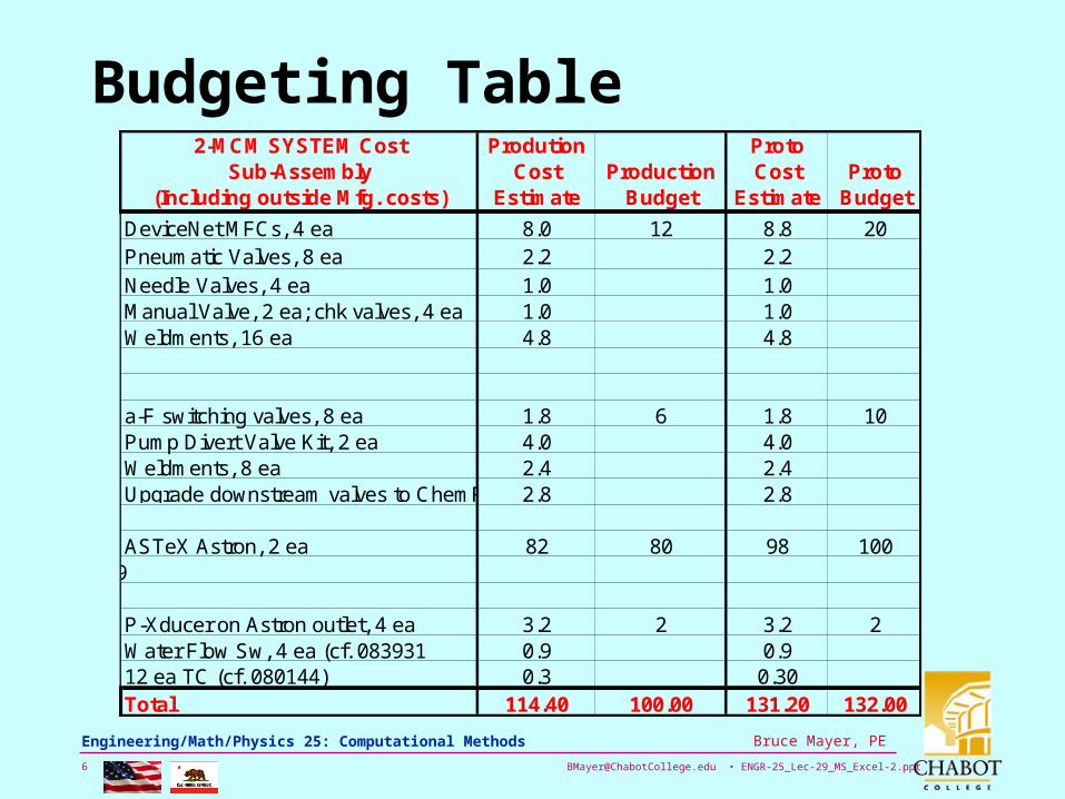
Budgeting Table2-MCM SYSTEM Cost
Sub-Assembly (Including outside Mfg. costs)
Prodution Cost
EstimateProduction
Budget
Proto Cost
EstimateProto
Budget
DeviceNet MFCs, 4 ea 8.0 12 8.8 20Pneumatic Valves, 8 ea 2.2 2.2Needle Valves, 4 ea 1.0 1.0Manual Valve, 2 ea; chk valves, 4 ea 1.0 1.0Weldments, 16 ea 4.8 4.8
a-F switching valves, 8 ea 1.8 6 1.8 10Pump Divert Valve Kit, 2 ea 4.0 4.0Weldments, 8 ea 2.4 2.4Upgrade downstream valves to ChemRaz 2.8 2.8
ASTeX Astron, 2 ea 82 80 98 100ASTeX qte SW031599
P-Xducer on Astron outlet, 4 ea 3.2 2 3.2 2Water Flow Sw, 4 ea (cf. 083931 0.9 0.912 ea TC (cf. 080144) 0.3 0.30Total 114.40 100.00 131.20 132.00

[email protected] • ENGR-25_Lec-29_MS_Excel-2.ppt7
Bruce Mayer, PE Engineering/Math/Physics 25: Computational Methods
Table Construction Demo
Fall: Course TitleCourse No. Units Spring: Course TitleCourse No.UnitsVector Mechanics - DynamicsME 104 3 Technical Communication E 190 3ThermodynamicsME 105 3 Fluid MechanicsME 106 3
Year 3 Mechanics of MaterialsCE 130 3 Mechanical Behavior of Materials ME C124 3Computational MethodsE77 3 Orthopedic Biomechanics ME C176 3Electronic Techniques EE100 3 Game Theory ECON C110 3
Total Units 15 Total Units 15
Fall: Course Title Course No. Units Spring: Course Title Course No. Units
Vector Mechanics - Dynamics ME 104 3 Technical Communication E 190 3Thermodynamics ME 105 3 Fluid Mechanics ME 106 3Mechanics of Materials CE 130 3 Mechanical Behavior of Materials ME C124 3Computational Methods E77 3 Orthopedic Biomechanics ME C176 3Electronic Techniques EE100 3 Game Theory ECON C110 3
Total Units 15 Total Units 15
Year 3

[email protected] • ENGR-25_Lec-29_MS_Excel-2.ppt8
Bruce Mayer, PE Engineering/Math/Physics 25: Computational Methods
Charts and Graphs
Carefully The Select the TYPE of Chart• Different Charts Convey Different Info
Make Clear and Easy to Read• Large Fonts• Good Contrast
– Light-on-Dark or Dark-on-Light
Include Legend Unless Info in Title Label All Axes, Including Units
[email protected] • ENGR-25_Lec-29_MS_Excel-2.ppt9
Bruce Mayer, PE Engineering/Math/Physics 25: Computational Methods
Charts & Graphs cont
Where Appropriate Annotate or Mark points/regions of Interest with Arrows, Ovals, or Text
There are 11 different chart types in Microsoft Excel (and several variations of each type) • This Covers 99.9% of the Chart Types That
Most Engineers will need• Consider Next the Criteria for application

[email protected] • ENGR-25_Lec-29_MS_Excel-2.ppt10
Bruce Mayer, PE Engineering/Math/Physics 25: Computational Methods
The 11 MS Excel Chart Types

[email protected] • ENGR-25_Lec-29_MS_Excel-2.ppt11
Bruce Mayer, PE Engineering/Math/Physics 25: Computational Methods
MS Excel Charts
Area Chart• An area chart
emphasizes the magnitude of change over time. By displaying the sum of the plotted values, an area chart also shows the relationship of parts to a whole.

[email protected] • ENGR-25_Lec-29_MS_Excel-2.ppt12
Bruce Mayer, PE Engineering/Math/Physics 25: Computational Methods
MS Excel Charts
Bar Chart• A bar chart
illustrates comparisons among individual items. Categories are organized vertically, values horizontally, to focus on comparing values and to place LESS emphasis on time. Stacked bar charts showthe relationship of individual items to the whole.
Alignment Effectiveness vs. No. of Calibration Points
27.05
25.00
23.11
21.08
0 5 10 15 20 25 30
65
43
Nu
mb
er
of
Alig
nm
en
t P
oin
ts
Aligned vs. Unaligned Effectiveness file = Align_CoOrd_Test_020320.xls
0 2 4 6 8 10 12 14
N
S
E
W
Production Volume (tons)Re
gion
Milk
IceCream
Chese

[email protected] • ENGR-25_Lec-29_MS_Excel-2.ppt13
Bruce Mayer, PE Engineering/Math/Physics 25: Computational Methods
MS Excel Charts Column Chart
• A column chart shows data changes over a period of time or illustrates comparisons among items. Categories are organized horizontally, values vertically, to emphasize variation over time. Stacked column charts show the relationship of individual items to the whole.

[email protected] • ENGR-25_Lec-29_MS_Excel-2.ppt14
Bruce Mayer, PE Engineering/Math/Physics 25: Computational Methods
MS Excel Charts
Line Chart• A line chart shows trends in data at equal
intervals. Although line charts are similar to area charts, line charts emphasize time flow and the rate of change, rather than the amount of change or the magnitude of values.

[email protected] • ENGR-25_Lec-29_MS_Excel-2.ppt15
Bruce Mayer, PE Engineering/Math/Physics 25: Computational Methods
MS Excel Charts
Pie Chart• A pie chart shows the proportional size of
items that make up a data series to the sum of the items.
• It always shows only one data series and is useful when you want to emphasize a significant element
[email protected] • ENGR-25_Lec-29_MS_Excel-2.ppt16
Bruce Mayer, PE Engineering/Math/Physics 25: Computational Methods
MS Excel Charts
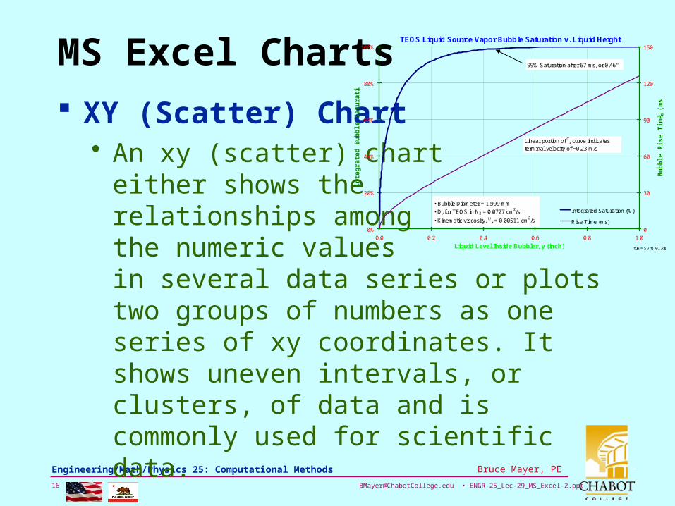
XY (Scatter) Chart• An xy (scatter) chart
either shows the relationships among the numeric values in several data series or plots two groups of numbers as one series of xy coordinates. It shows uneven intervals, or clusters, of data and is commonly used for scientific data.
TEOS Liquid Source Vapor Bubble Saturation v. Liquid Height
0%
20%
40%
60%
80%
100%
0.0 0.2 0.4 0.6 0.8 1.0
Liquid Level Inside Bubbler, y (inch)
Inte
gra
ted
Bu
bb
le S
atu
rati
on
, Sv
0
30
60
90
120
150
Bu
bb
le R
ise
Tim
e,
r (m
s)
Integrated Saturation (%)
Rise Time (ms)
file = Sv(t)_01.xls
• Bubble Diameter = 1.999 mm
• Dv for TEOS in N2 = 0.0727 cm2/s
• Kinematic viscosity,, = 0.00511 cm2/s
99% Saturation after 67 ms, or 0.46"
Linear portion of r curve indicatesterminal velocity of ~0.23 m/s

[email protected] • ENGR-25_Lec-29_MS_Excel-2.ppt17
Bruce Mayer, PE Engineering/Math/Physics 25: Computational Methods
MS Excel Charts
Doughnut Chart• Like a pie chart, a doughnut chart shows
the relationship of parts to a whole, but it can contain more than one data series. Each ring of the doughnut chart represents a data series
• Basically nestedPie-Charts

[email protected] • ENGR-25_Lec-29_MS_Excel-2.ppt18
Bruce Mayer, PE Engineering/Math/Physics 25: Computational Methods
MS Excel Charts
Radar Chart• In a radar chart, each category has its own
value axis radiating from the center point. Lines connect all the values in the same series. A radar chart compares the aggregate values of a number of data series.

[email protected] • ENGR-25_Lec-29_MS_Excel-2.ppt19
Bruce Mayer, PE Engineering/Math/Physics 25: Computational Methods
MS Excel Charts
Surface Chart• A 3D surface chart is useful when you want
to find optimum combinations between two sets of data. As in a topographic map, colors and patternsindicate areas thatare in the samerange of values.
5060
7080
90100
200250
300350
400450
500550
600650
700
4.4%
4.6%
4.8%
5.0%
5.2%
5.4%
5.6%
5.8%
6.0%
6.2%
6.4%
6.6%
6.8%
Cha
nge
in B
ubbl
er O
utpu
t (%
/°C
)
Bubbler Temperature (°C)
Chamber Pressure (Torr)
TEOS Bubbler Vapor Generator Temp Sensitivity
file =VapGen_T-P_Sens.xls

[email protected] • ENGR-25_Lec-29_MS_Excel-2.ppt20
Bruce Mayer, PE Engineering/Math/Physics 25: Computational Methods
MS Excel Charts
Bubble Chart• A bubble chart is a type of xy (scatter)
chart. The size of the data marker indicates the value of a third variable.
4-Pt Aligned Error Mag vs. Position • KLARFF Wafer CZHA
-12
-8
-4
0
4
8
12
-4 -3 -2 -1 0 1 2 3 4
Xindex
Yin
de
x
NOTES• OTA-2100• 200mm IBM Wafer CZHA.001 • Test Date = 20Mar02• Aligned Avg Error Vector = 8.52 µm
file = Align_CoOrd_Test_020320.xls
[email protected] • ENGR-25_Lec-29_MS_Excel-2.ppt21
Bruce Mayer, PE Engineering/Math/Physics 25: Computational Methods
MS Excel Charts
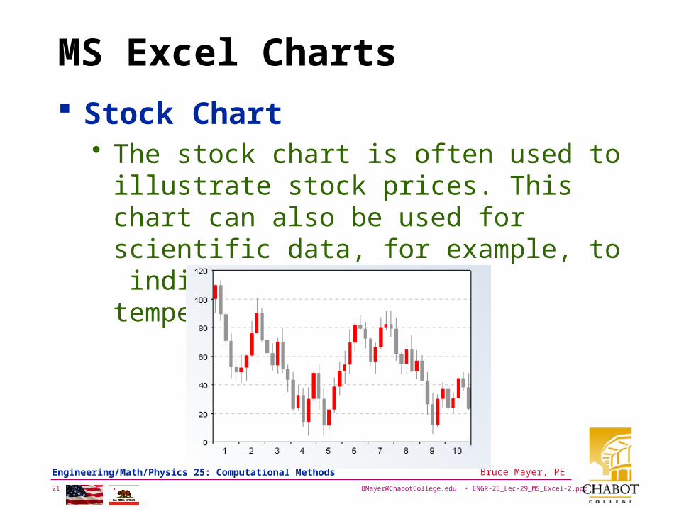
Stock Chart• The stock chart is often used to illustrate
stock prices. This chart can also be used for scientific data, for example, to indicate temperature changes
[email protected] • ENGR-25_Lec-29_MS_Excel-2.ppt22
Bruce Mayer, PE Engineering/Math/Physics 25: Computational Methods
MS Excel Charts
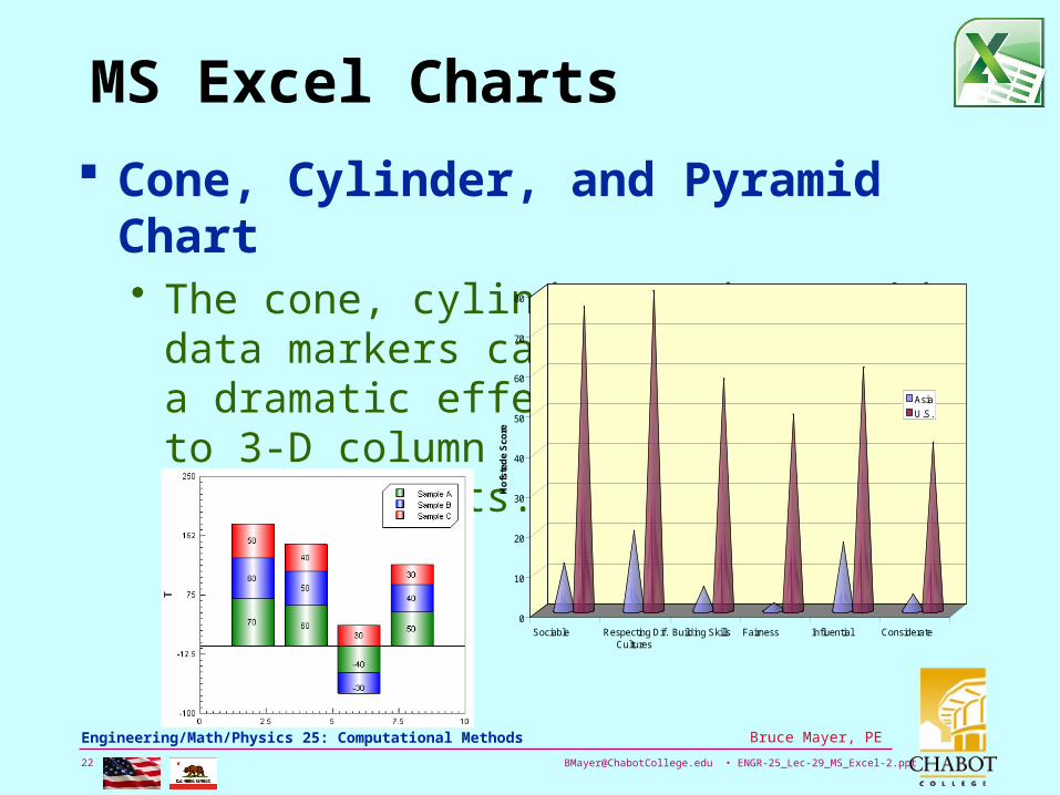
Cone, Cylinder, and Pyramid Chart • The cone, cylinder, and pyramid data
markers can lend a dramatic effect to 3-D column and bar charts.
0
10
20
30
40
50
60
70
80
Ho
fste
de
Sco
re
Sociable Respecting Dif.Cultures
Building Skills Fairness Influential Considerate
Asia
U.S.
[email protected] • ENGR-25_Lec-29_MS_Excel-2.ppt23
Bruce Mayer, PE Engineering/Math/Physics 25: Computational Methods
Graph Construction Demo
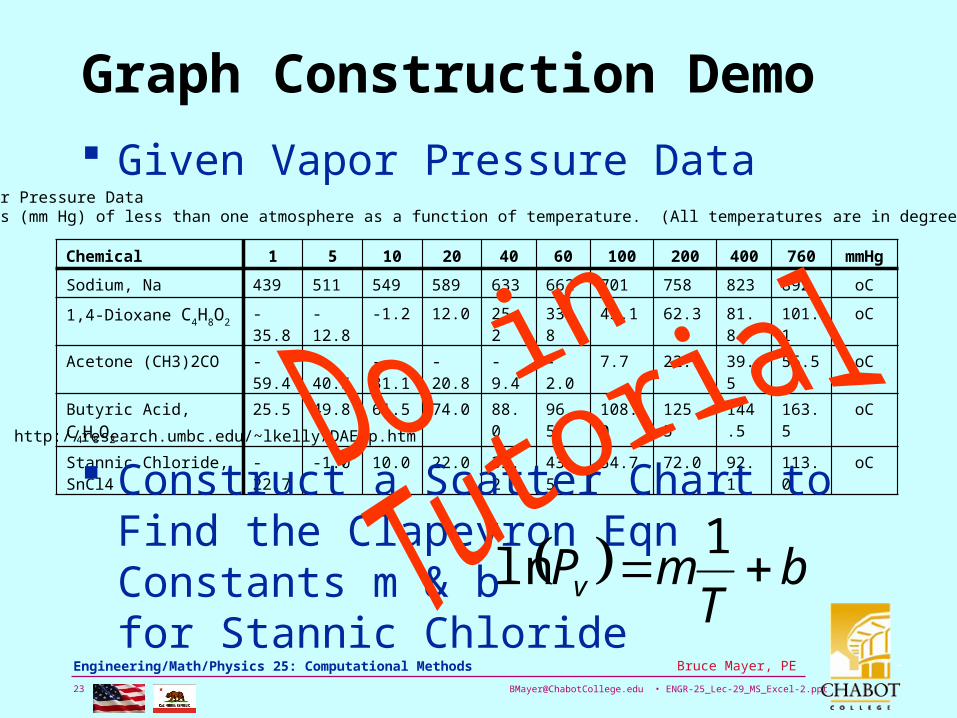
TABLE I: Vapor Pressure DataVapor pressures (mm Hg) of less than one atmosphere as a function of temperature. (All temperatures are in degrees Celsius)
Chemical 1 5 10 20 40 60 100 200 400 760 mmHg
Sodium, Na 439 511 549 589 633 662 701 758 823 892 oC
1,4-Dioxane C4H8O2-35.8 -12.8 -1.2 12.0 25.2 33.8 45.1 62.3 81.8 101.1 oC
Acetone (CH3)2CO -59.4 -40.5 -31.1 -20.8 -9.4 -2.0 7.7 22.7 39.5 56.5 oC
Butyric Acid, C4H8O225.5 49.8 61.5 74.0 88.0 96.5 108.0 125.5 144.5 163.5 oC
Stannic Chloride, SnCl4 -22.7 -1.0 10.0 22.0 35.2 43.5 54.7 72.0 92.1 113.0 oC
http://research.umbc.edu/~lkelly/DAExp.htm
Given Vapor Pressure Data
Construct a Scatter Chart to Find the Clapeyron Eqn Constants m & bfor Stannic Chloride
bT
mPv 1
ln
[email protected] • ENGR-25_Lec-29_MS_Excel-2.ppt24
Bruce Mayer, PE Engineering/Math/Physics 25: Computational Methods
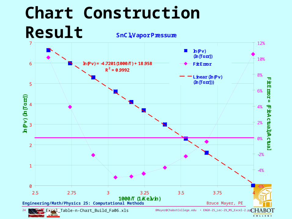
Chart Construction ResultSnCl4Vapor Pressure
ln(Pv) = -4.7201(1000/T) + 18.958
R2 = 0.9992
0
1
2
3
4
5
6
7
2.5 2.75 3 3.25 3.5 3.75 41000/T (1/Kelvin)
ln(P
v) (
ln[T
orr
])
-6%
-4%
-2%
0%
2%
4%
6%
8%
10%
12%
Fit E
rror =
(Fit-A
ctua
l)/Actu
al
ln(Pv)(ln[Torr])
Fit Error
Linear (ln(Pv)(ln[Torr]))
Demo_Excel_Table-n-Chart_Build_Fa06.xls
[email protected] • ENGR-25_Lec-29_MS_Excel-2.ppt25
Bruce Mayer, PE Engineering/Math/Physics 25: Computational Methods
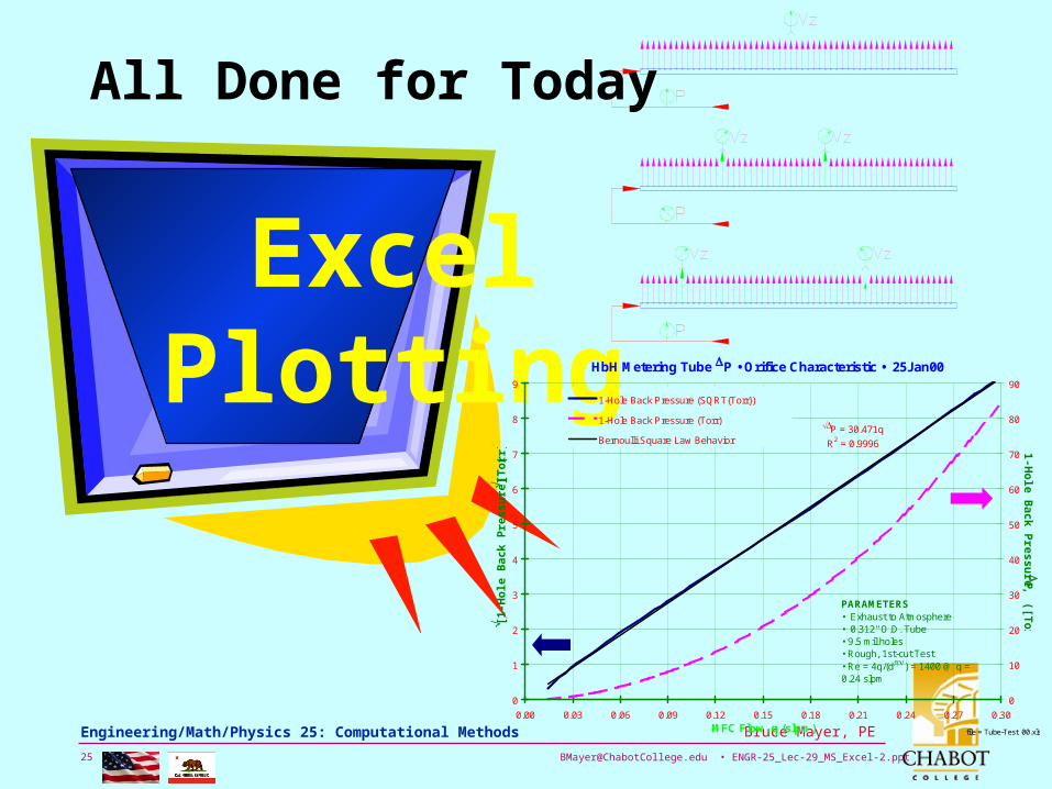
All Done for Today
ExcelPlotting HbH Metering Tube P • Orifice Characteristic • 25Jan00
P = 30.471q
R2 = 0.9996
0
1
2
3
4
5
6
7
8
9
0.00 0.03 0.06 0.09 0.12 0.15 0.18 0.21 0.24 0.27 0.30MFC Flow, q (slpm)
[1
-Ho
le B
ac
k P
res
su
re]
( [
Torr
])
0
10
20
30
40
50
60
70
80
90
1-H
ole
Ba
ck
Pre
ss
ure
, P ([To
rr)
1-Hole Back Pressure (SQRT{Torr})
1-Hole Back Pressure (Torr)
Bernoulli Square Law Behavior
file = Tube-Test_00.xls
PARAMETERS• Exhaust to Atmosphere• 0.312" O.D. Tube• 9.5 mil holes• Rough, 1st-cut Test• Re = 4q/(d) = 1400 @ q = 0.24 slpm
[email protected] • ENGR-25_Lec-29_MS_Excel-2.ppt26
Bruce Mayer, PE Engineering/Math/Physics 25: Computational Methods
Bruce Mayer, PELicensed Electrical & Mechanical Engineer
Engr/Math/Physics 25
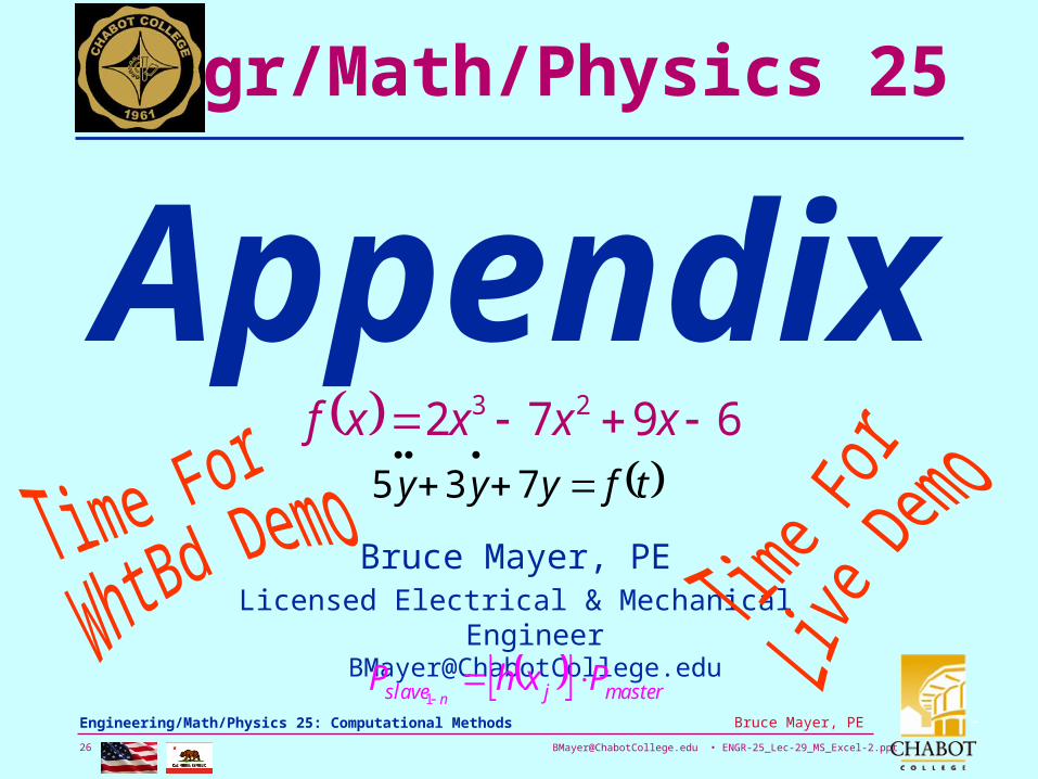
Appendix
6972 23 xxxxf tfyyy
735
masterjslave PxhPn
1
[email protected] • ENGR-25_Lec-29_MS_Excel-2.ppt27
Bruce Mayer, PE Engineering/Math/Physics 25: Computational Methods
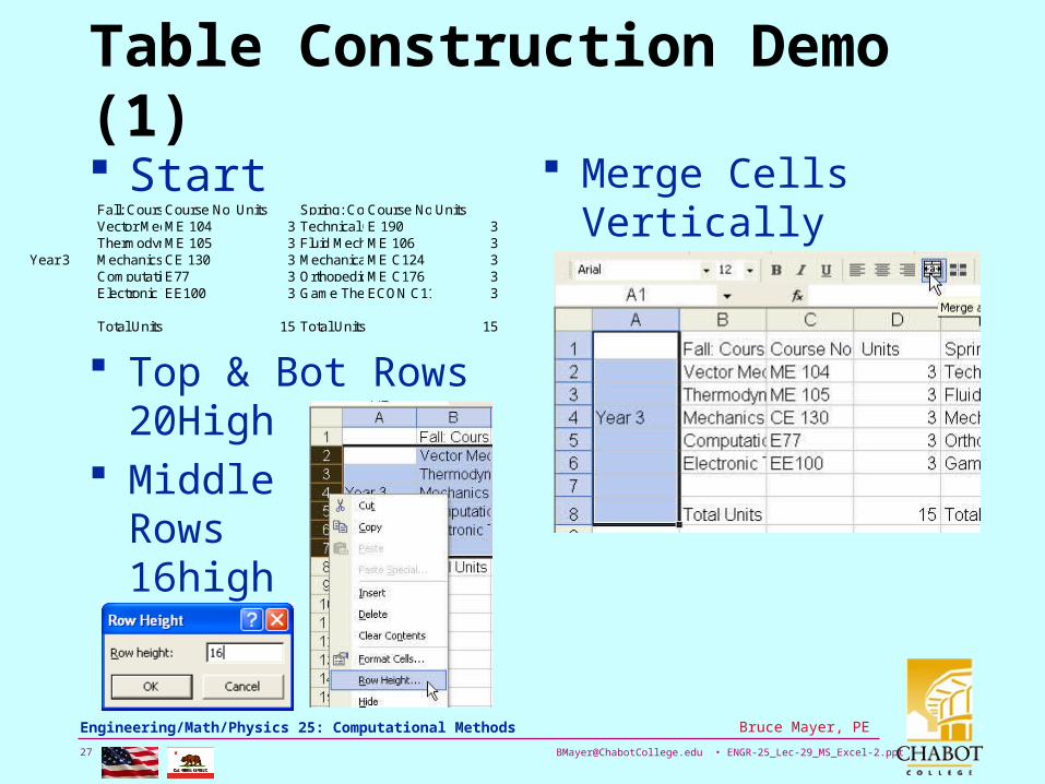
Table Construction Demo (1)
StartFall: Course TitleCourse No. Units Spring: Course TitleCourse No.UnitsVector Mechanics - DynamicsME 104 3 Technical Communication E 190 3ThermodynamicsME 105 3 Fluid MechanicsME 106 3
Year 3 Mechanics of MaterialsCE 130 3 Mechanical Behavior of Materials ME C124 3Computational MethodsE77 3 Orthopedic Biomechanics ME C176 3Electronic Techniques EE100 3 Game Theory ECON C110 3
Total Units 15 Total Units 15
Top & Bot Rows 20High
Middle Rows 16high
Merge Cells Vertically
[email protected] • ENGR-25_Lec-29_MS_Excel-2.ppt28
Bruce Mayer, PE Engineering/Math/Physics 25: Computational Methods
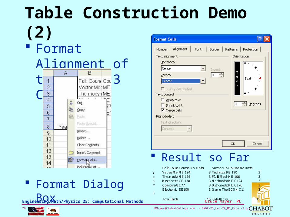
Table Construction Demo (2)
Format Alignment of the “Year 3 Cell
Result so Far
Format Dialog Box
Fall: Course TitleCourse No. Units Spring: Course TitleCourse No.UnitsVector Mechanics - DynamicsME 104 3 Technical Communication E 190 3ThermodynamicsME 105 3 Fluid MechanicsME 106 3Mechanics of MaterialsCE 130 3 Mechanical Behavior of Materials ME C124 3Computational MethodsE77 3 Orthopedic Biomechanics ME C176 3Electronic Techniques EE100 3 Game Theory ECON C110 3
Total Units 15 Total Units 15
Year 3
[email protected] • ENGR-25_Lec-29_MS_Excel-2.ppt29
Bruce Mayer, PE Engineering/Math/Physics 25: Computational Methods
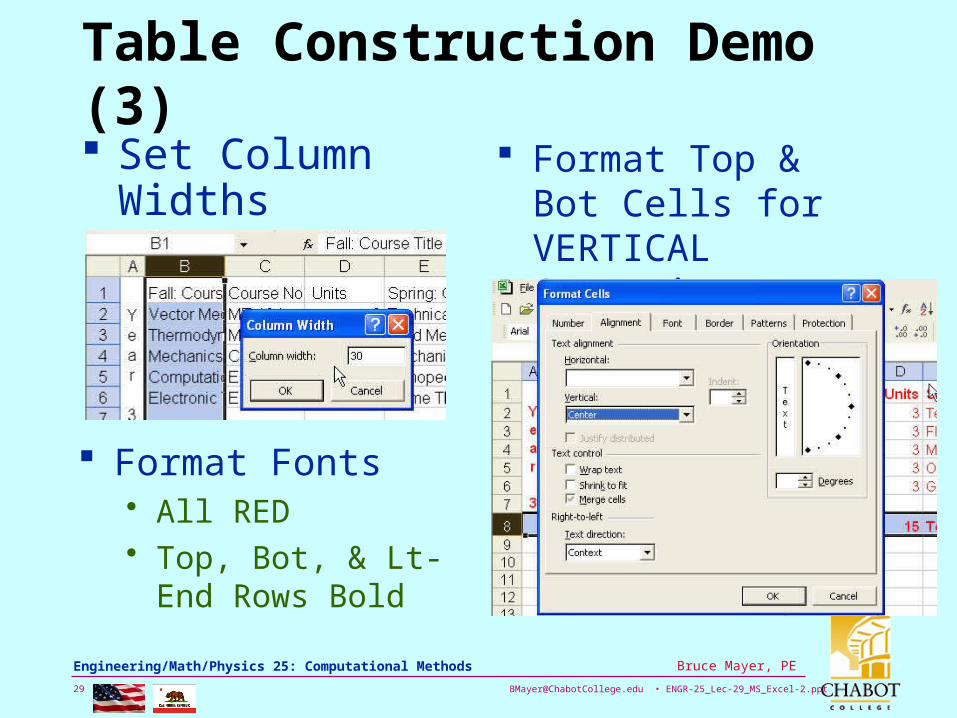
Table Construction Demo (3) Set Column
Widths• 2, 30, 11, 5, 30,
11, 5
Format Fonts• All RED• Top, Bot, & Lt-End
Rows Bold
Format Top & Bot Cells for VERTICAL Centering

[email protected] • ENGR-25_Lec-29_MS_Excel-2.ppt30
Bruce Mayer, PE Engineering/Math/Physics 25: Computational Methods
Table Construction Demo (4) Set Border Color
to Blue Grid INSIDE blue
[email protected] • ENGR-25_Lec-29_MS_Excel-2.ppt31
Bruce Mayer, PE Engineering/Math/Physics 25: Computational Methods
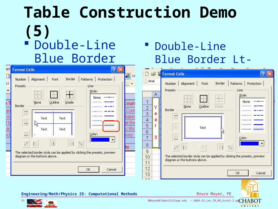
Table Construction Demo (5) Double-Line Blue
Border Outside Double-Line Blue
Border Lt-Vert Cell

[email protected] • ENGR-25_Lec-29_MS_Excel-2.ppt32
Bruce Mayer, PE Engineering/Math/Physics 25: Computational Methods
Table Construction Demo (6)
Double-Line Blue Border RemainderFall: Course Title Course No. Units Spring: Course Title Course No. Units
Vector Mechanics - Dynamics ME 104 3 Technical Communication E 190 3Thermodynamics ME 105 3 Fluid Mechanics ME 106 3Mechanics of Materials CE 130 3 Mechanical Behavior of Materials ME C124 3Computational Methods E77 3 Orthopedic Biomechanics ME C176 3Electronic Techniques EE100 3 Game Theory ECON C110 3
Total Units 15 Total Units 15
Year 3
[email protected] • ENGR-25_Lec-29_MS_Excel-2.ppt33
Bruce Mayer, PE Engineering/Math/Physics 25: Computational Methods
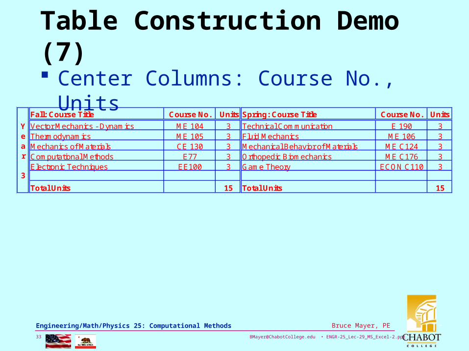
Table Construction Demo (7)
Center Columns: Course No., Units
Fall: Course Title Course No. Units Spring: Course Title Course No. Units
Vector Mechanics - Dynamics ME 104 3 Technical Communication E 190 3Thermodynamics ME 105 3 Fluid Mechanics ME 106 3Mechanics of Materials CE 130 3 Mechanical Behavior of Materials ME C124 3Computational Methods E77 3 Orthopedic Biomechanics ME C176 3Electronic Techniques EE100 3 Game Theory ECON C110 3
Total Units 15 Total Units 15
Year 3
[email protected] • ENGR-25_Lec-29_MS_Excel-2.ppt34
Bruce Mayer, PE Engineering/Math/Physics 25: Computational Methods
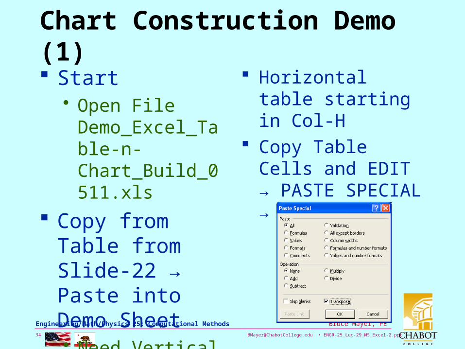
Chart Construction Demo (1)
Start • Open File
Demo_Excel_Table-n-Chart_Build_0511.xls
Copy from Table from Slide-22 → Paste into Demo Sheet • Need Vertical
Data
Horizontal table starting in Col-H
Copy Table Cells and EDIT → PASTE SPECIAL → transpose

[email protected] • ENGR-25_Lec-29_MS_Excel-2.ppt35
Bruce Mayer, PE Engineering/Math/Physics 25: Computational Methods
Chart Construction Demo (2)
Result after Transpose Paste

[email protected] • ENGR-25_Lec-29_MS_Excel-2.ppt36
Bruce Mayer, PE Engineering/Math/Physics 25: Computational Methods
Chart Construction Demo (3)
Archive Data• Make Scratch
WorkSheet; Xfer horizontal Table to to this sheet
Edit Worksheet• Adjust Headings• Delete Cols other
Than SnCl4• Move Remaining
to Right

[email protected] • ENGR-25_Lec-29_MS_Excel-2.ppt37
Bruce Mayer, PE Engineering/Math/Physics 25: Computational Methods
Chart Construction Demo (4)
Place in cols A & B• 1000/T; T in
Kelvins• Ln(Pv)
After Filling A & B
Formula for Col-B• =LN(E8)

[email protected] • ENGR-25_Lec-29_MS_Excel-2.ppt38
Bruce Mayer, PE Engineering/Math/Physics 25: Computational Methods
Chart Construction Demo (5)
Now need to Sort the Data with the indep var (1000/T) in ASCENDING ORDER• DATA → SORT

[email protected] • ENGR-25_Lec-29_MS_Excel-2.ppt39
Bruce Mayer, PE Engineering/Math/Physics 25: Computational Methods
Chart Construction Demo (6)
Highlight/Select Data to Plot
Invoke Chart Wizard
[email protected] • ENGR-25_Lec-29_MS_Excel-2.ppt40
Bruce Mayer, PE Engineering/Math/Physics 25: Computational Methods
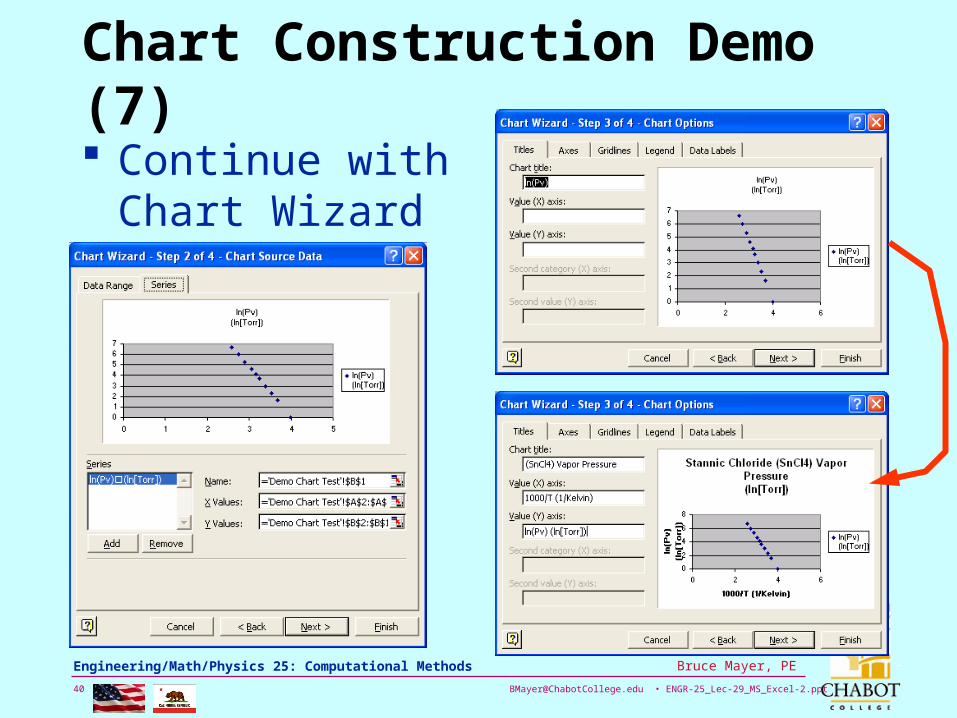
Chart Construction Demo (7)
Continue with Chart Wizard
[email protected] • ENGR-25_Lec-29_MS_Excel-2.ppt41
Bruce Mayer, PE Engineering/Math/Physics 25: Computational Methods
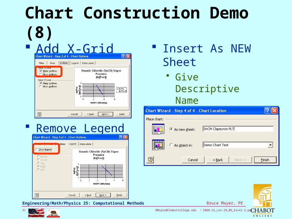
Chart Construction Demo (8)
Add X-Grid Lines
Remove Legend
Insert As NEW Sheet• Give Descriptive
Name

[email protected] • ENGR-25_Lec-29_MS_Excel-2.ppt42
Bruce Mayer, PE Engineering/Math/Physics 25: Computational Methods
Chart Construction Demo (9)
Stannic Chloride (SnCl4) Vapor Pressure(ln[Torr])
0
1
2
3
4
5
6
7
0 0.5 1 1.5 2 2.5 3 3.5 4 4.5
1000/T (1/Kelvin)
ln(P
v) (
ln[T
orr
])
Chart Wizard Result
Change• X-axis Scale: 2.5-4• Shorten Title• Clear BackGround• Lager, Sq Data Markers• GridLine & Text Colors

[email protected] • ENGR-25_Lec-29_MS_Excel-2.ppt43
Bruce Mayer, PE Engineering/Math/Physics 25: Computational Methods
Chart Construction Demo (10)
Select Chart Area ThenRight-Clik
Select X-axis, Ther Right-Clik

[email protected] • ENGR-25_Lec-29_MS_Excel-2.ppt44
Bruce Mayer, PE Engineering/Math/Physics 25: Computational Methods
Chart Construction Demo (11)
Select Grid Lines, Rt-Clik, Chg Colors
Select Data Series, Rt-Clik, Chg Marker

[email protected] • ENGR-25_Lec-29_MS_Excel-2.ppt45
Bruce Mayer, PE Engineering/Math/Physics 25: Computational Methods
Chart Construction Demo (12)
Position Labels at Page Edges → Stretch-Out Plot Area

[email protected] • ENGR-25_Lec-29_MS_Excel-2.ppt46
Bruce Mayer, PE Engineering/Math/Physics 25: Computational Methods
Chart Construction Demo (13)
Chart Fine-Tuning ResultSnCl4Vapor Pressure
0
1
2
3
4
5
6
7
2.5 2.75 3 3.25 3.5 3.75 41000/T (1/Kelvin)
ln(P
v) (
ln[T
orr
])
Add TrendLine to find Clapeyron m &b Constants

[email protected] • ENGR-25_Lec-29_MS_Excel-2.ppt47
Bruce Mayer, PE Engineering/Math/Physics 25: Computational Methods
Chart Construction Demo (14)
Select Data Series, Rt-Clik, Add TrendLn
Select: Linear, Display Parameters

[email protected] • ENGR-25_Lec-29_MS_Excel-2.ppt48
Bruce Mayer, PE Engineering/Math/Physics 25: Computational Methods
Chart Construction Demo (15)
Fine Tune TrendLine Form & DisplaySnCl4Vapor Pressure
y = -4.7201x + 18.958
R2 = 0.99920
1
2
3
4
5
6
7
8
2.5 2.75 3 3.25 3.5 3.75 41000/T (1/Kelvin)
ln(P
v) (
ln[T
orr
])
SnCl4Vapor Pressure
ln(Pv) = -4.7201(1000/T) + 18.958
R2 = 0.9992
0
1
2
3
4
5
6
7
8
2.5 2.75 3 3.25 3.5 3.75 4
1000/T (1/Kelvin)
ln(P
v) (
ln[T
orr
])
Done with Plot; and have determined m & b by Trendline• Note that the Fit is Excellent;
R2 = 99.92%
[email protected] • ENGR-25_Lec-29_MS_Excel-2.ppt49
Bruce Mayer, PE Engineering/Math/Physics 25: Computational Methods
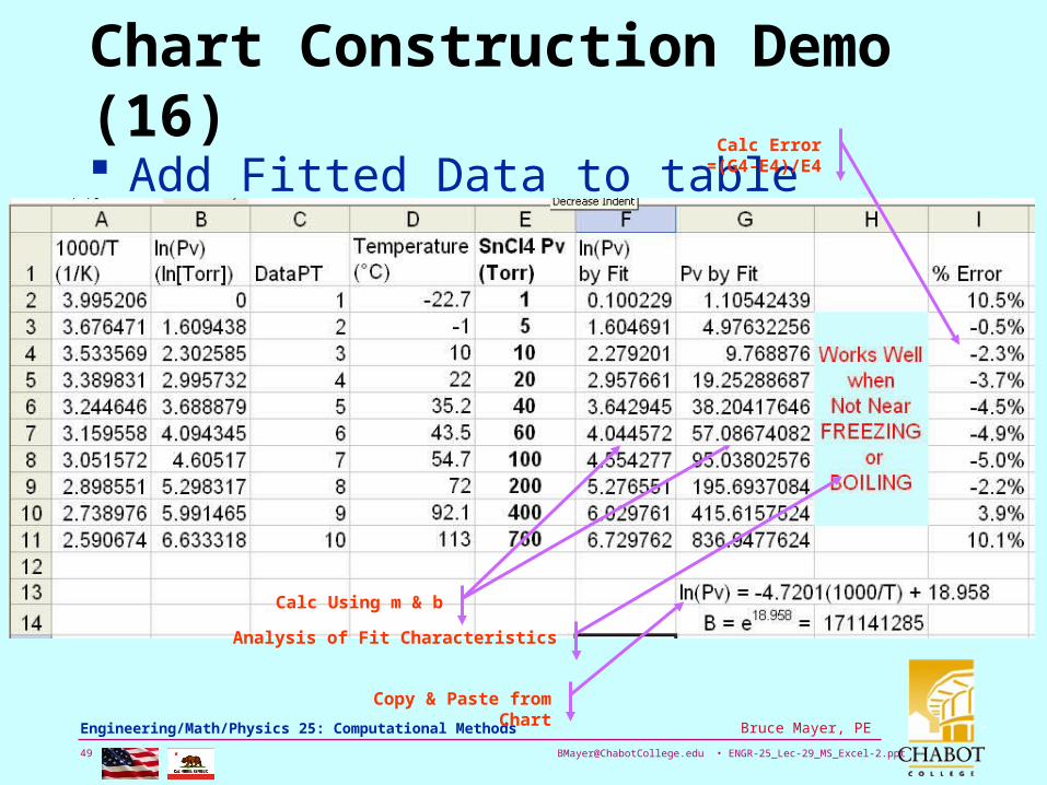
Chart Construction Demo (16)
Add Fitted Data to table
Copy & Paste from Chart
Calc Using m & b
Analysis of Fit Characteristics
Calc Error=(G4-E4)/E4
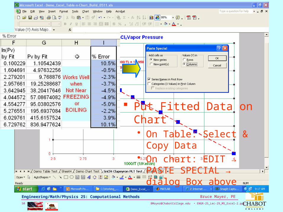
[email protected] • ENGR-25_Lec-29_MS_Excel-2.ppt50
Bruce Mayer, PE Engineering/Math/Physics 25: Computational Methods
Put Fitted Data on Chart• On Table: Select & Copy
Data• On chart: EDIT → PASTE
SPECIAL → dialog Box above

[email protected] • ENGR-25_Lec-29_MS_Excel-2.ppt51
Bruce Mayer, PE Engineering/Math/Physics 25: Computational Methods
Chart Construction Demo (17)
Fine Tune Two-Variable DisplaySnCl4Vapor Pressure
ln(Pv) = -4.7201(1000/T) + 18.958
R2 = 0.9992
-1
0
1
2
3
4
5
6
7
8
2.5 2.75 3 3.25 3.5 3.75 4
1000/T (1/Kelvin)
ln(P
v) (
ln[T
orr
])
Error Data Series
To Make Error Data More Visible Show using SECONDARY Axis at Right

[email protected] • ENGR-25_Lec-29_MS_Excel-2.ppt52
Bruce Mayer, PE Engineering/Math/Physics 25: Computational Methods
Chart Construction Demo (18)SnCl4Vapor Pressure
ln(Pv) = -4.7201(1000/T) + 18.958
R2 = 0.9992
0
1
2
3
4
5
6
7
8
2.5 2.75 3 3.25 3.5 3.75 4
1000/T (1/Kelvin)
ln(P
v) (
ln[T
orr
])
-6.0%
-4.0%
-2.0%
0.0%
2.0%
4.0%
6.0%
8.0%
10.0%
12.0%

[email protected] • ENGR-25_Lec-29_MS_Excel-2.ppt53
Bruce Mayer, PE Engineering/Math/Physics 25: Computational Methods
Chart Construction Demo (19)
Fine Tune Two-Axes Display

[email protected] • ENGR-25_Lec-29_MS_Excel-2.ppt54
Bruce Mayer, PE Engineering/Math/Physics 25: Computational Methods
Chart Construction Demo (20)SnCl4Vapor Pressure
ln(Pv) = -4.7201(1000/T) + 18.958
R2 = 0.9992
0
1
2
3
4
5
6
7
2.5 2.75 3 3.25 3.5 3.75 41000/T (1/Kelvin)
ln(P
v) (
ln[T
orr
])
-6%
-4%
-2%
0%
2%
4%
6%
8%
10%
12%
Fit E
rror =
(Fit-A
ctua
l)/Actu
al
ln(Pv)(ln[Torr])
Fit Error
Linear (ln(Pv)(ln[Torr]))

[email protected] • ENGR-25_Lec-29_MS_Excel-2.ppt55
Bruce Mayer, PE Engineering/Math/Physics 25: Computational Methods
Nice Chart

[email protected] • ENGR-25_Lec-29_MS_Excel-2.ppt56
Bruce Mayer, PE Engineering/Math/Physics 25: Computational Methods
Coefficient of Correlation
The coefficient of correlation is an indication of how well the linear relationship determined by the method of least squares fits the data set.
The equation for the coefficient of correlation is:
2i
2i
2i
2i
iiii
)y()yn()x()xn(
)y)(x()yxn(R

[email protected] • ENGR-25_Lec-29_MS_Excel-2.ppt57
Bruce Mayer, PE Engineering/Math/Physics 25: Computational Methods
Interpretation of R
If R is 0, the points are so scattered that the regression line does not help predict y for a given x.
If R is +1 (positive slope) or –1 (negative slope), the points actually lie on a straight line so almost perfect predictions of y for a given x can be made using the regression line.
[email protected] • ENGR-25_Lec-29_MS_Excel-2.ppt58
Bruce Mayer, PE Engineering/Math/Physics 25: Computational Methods
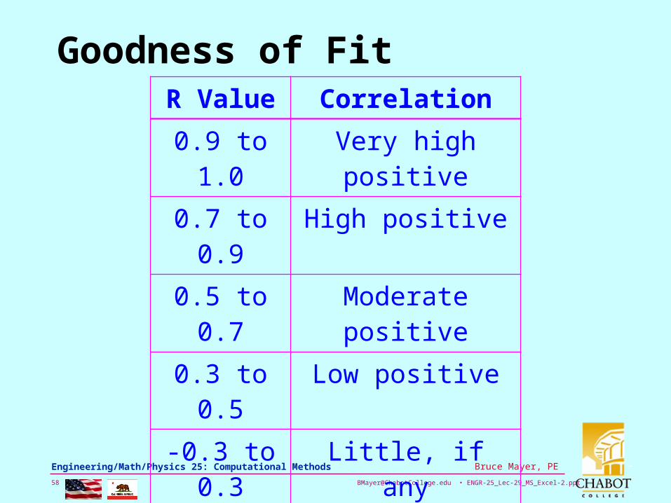
Goodness of FitR Value Correlation
0.9 to 1.0 Very high positive
0.7 to 0.9 High positive
0.5 to 0.7 Moderate positive
0.3 to 0.5 Low positive
-0.3 to 0.3 Little, if any
-0.5 to -0.3 Low negative
-0.7 to -0.5 Moderate negative
-0.9 to -0.7 High negative
-1.0 to -0.9 Very high negative

[email protected] • ENGR-25_Lec-29_MS_Excel-2.ppt59
Bruce Mayer, PE Engineering/Math/Physics 25: Computational Methods