Bluman: Elamentary 7.The Normal Distribution Text The ... handout/Chapters 7 and 8.pdf · 252...
88
Bluman: Elamentary 7. The Normal Distribution Text Statistics: AStep byStep Approach, Fourth Edition © The McGraw-Hili Companies, 2001 .;" '.> . l.." .,.:,., .. '/-"'!.
-
Upload
phungxuyen -
Category
Documents
-
view
243 -
download
0
Transcript of Bluman: Elamentary 7.The Normal Distribution Text The ... handout/Chapters 7 and 8.pdf · 252...
Bluman: Elamentary 7.The Normal Distribution TextStatistics: AStep byStepApproach, Fourth Edition
© The McGraw-HiliCompanies, 2001
.;"
:':':"",:<':~':"; '.>. l.."
.,.:,.,
..'/-"'!. ,:;:;,"':<>~:~:;;-'\:::
I) I Bluman: Elementary I 7.TheNOnl1al Distribution I TextStatistics: AStepbyStepApproach, Fourth Edition
© The McGraw-HiliCompanies, 2001
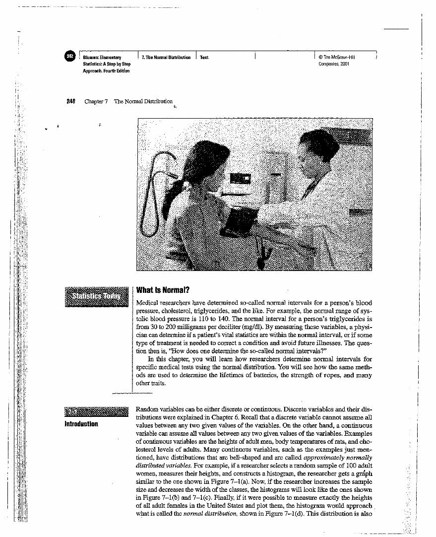
What Is Normal?Medical researchers have determined so-called normal intervals for a person's bloodpressure, cholesterol, triglycerides, and the like. For example, the normal range of systolic blood pressure is 110 to 140. The normal interval for a person's triglycerides isfrom 30 to 200 milligrams per deciliter (mg/dl). By measuring these variables, a physician can determine if a patient's vital statistics are within the normal interval, or if sometype of treatment is needed to correct a condition and avoid future illnesses. The question then is, "How does one determine the so-called normal intervals?"
In this chapter, you will learn how researchers determine normal intervals forspecific medical tests using the normal distribution. You will see how the same methods are used to determine the lifetimes of batteries, the strength of ropes, and manyother traits.
Random variables can be either discrete or continuous. Discrete variables and their distributions were explained in Chapter 6. Recall that a discrete variable cannot assume allvalues between any two given values of the variables. On the other hand, a continuousvariable can assume all values between any two given values of the variables. Examplesof continuous variables are the heights of adult men, body temperatures of rats, and cholesterollevels of adults. Many continuous variables, such as the examples just mentioned, have distributions that are bell-shaped and are called approximately normallydistributed variables. For example, if a researcher selects a random sample of 100 adultwomen, measures their heights, and constructs a histogram, the researcher gets a graphsimilar to the one shown in Figure 7-l(a). Now, if the researcher increases the samplesize and decreases the width of the classes, the histograms will look like the ones shownin Figure 7-l(b) and 7-l(c). Finally, if it were possible to measure exactly the heightsof all adult females in the United States and plot them, the histogram would approach.what is called the normal distribution, shown in Figure 7-1(d). This distribution is also
;,
248 Chapter 7 The NormalDistribution1:,
Introduction-

-c---- ~_
Normal and Skewed Distributions
";:1
:)
IW© The McGraw-HiliCompanies, 2001
Section 7-1 Introduction 249
IMode Median Mean
(e)Positively skewed
(b)Sample size increased and class width decreased
(d)Normal distribution forthe population
MeanMedianMode
(a)Normal
known as the bell curve or the Gaussian distribution, named for the German mathematician Carl Friedrich Gauss (1777-1855), who derived its equation.
No variable fits the normal distribution perfectly, since the normal distribution is a~
theoretical distribution. However, the normal distribution can be used to describe manyvariables, because the deviations from the normal distribution are very small. This concept will be explained further in the next section.
When the data values are evenly distributed about the mean, the distribution is saidto be symmetrical. Figure 7-2(a) shows a symmetrical distribution. When the majorityof the data values fall to the left or right of the mean, the distribution is said to beskewed. When the majority of the data values fall to the right of the mean, the distribution is said to be negatively or left skewed. The mean is to the left of the median, andthe mean and the median are to the left of the mode. See Figure 7-2(b). When the majority of the data values fall to the left of the mean, the distribution is said to be positively or right skewed. The mean falls to the right of the median and both the mean andthe median fall to the right of the mode. See Figure 7-2(c).
7.TheNormal Distribution Text
Mean Median Mode(b)Negatively skewed
(a)Random sample of100 women
(e) Sample size increased and class widthdecreased further
Bluman:ElementaryStatistics: AStepbyStepApproach, Fourth Edition
Histograms for theDistribution of Heights ofAdult Women
Figure 7-1
Oiljectivll 1. Identifydistributions as symmetricalorskewed.
Figure 7-2
---------

250 Chapter 7 The Normal Distribution
© The McGraw-HiliCompanies. 2001
where
e r« 2.718 (= means "is approximately equal to")
'IT =3.14
J.L = population mean
a = population standard deviation
This equation may look formidable, but in applied statistics, tables are used for specificproblems instead of the equation.
Another important aspect in applied statistics is that the area under the normal distribution curve is more important than thefrequencies. Therefore, when the normal distribution is pictured, the y axis, which indicates the frequencies, is sometimes omitted.
Circles can be different sizes, depending on their diameters (or radii) and can beused to represent wheels of different sizes. Likewise, normal curves have differentshapes and can be used to represent different variables.
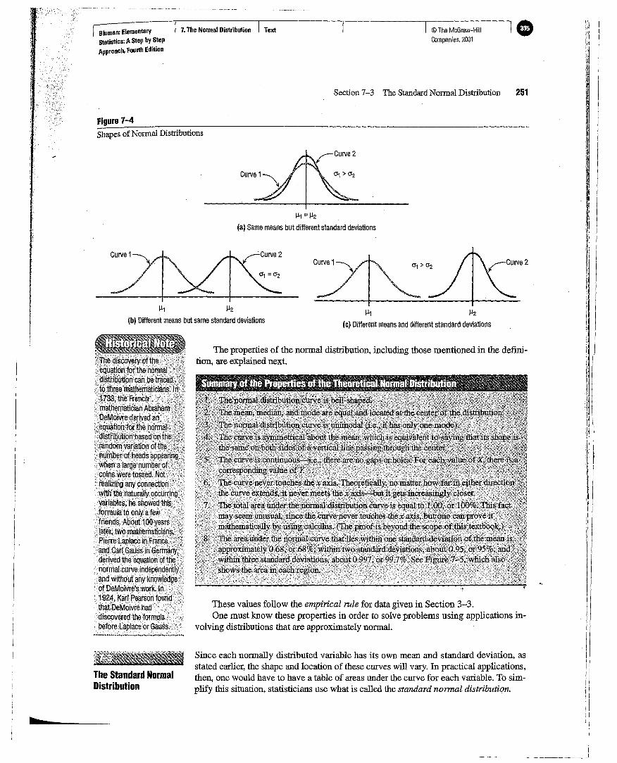
The shape and position of the normal distribution curve depend on two parameters, the mean and the standard deviation. Each normally distributed variablehas its own normal distribution curve, which depends on the values of the variable'smean and standard deviation. Figure 7-4(a) shows two normal distributions withthe same mean values but different standard deviations. The larger the standard deviation, the more dispersed, or spread out, the distribution is. Figure 7-4(b) shows twonormal distributions with the same standard deviation but with different means. Thesecurves have the same shapes but are located at different positions on the x axis. Figure 7-4(c) shows two normal distributions with different means and different standarddeviations.
In mathematics, curves can be represented by equations. For example, the equation ofthe circle shown in Figure 7-3 is x 2 + y2 = r 2, where r is the radius. The circle can beused to represent many physical objects, such as a wheel or a gear. Even though it is notpossible to manufacture a wheel that is perfectly round, the equation and the propertiesof the circle can be used to study the many aspects of the wheel, such as area, velocity,and acceleration. In a similar manner, the theoretical curve, called the normal distribution curve, can be used to study many variables that are not perfectly normally distributed but are nevertheless approximately normal.
The mathematical equation for the normal distribution is
~ , e-IX- JL)2f(2u')
y = u-yl21T
The "tail" of the curve indicates the direction of skewness (right is positive, leftnegative). This distribution can be compared with the one in Figure 3-1. Both types follow the same principles.
This chapter will present the properties of the normal distribution and discuss its applications. Then a very important theorem called the central limit theorem will be explained. Finally, the chapter will explain how the normal curve distribution can be usedas an approximation to other distributions, such as the binomial distribution. Since thebinomial distribution is a discrete distribution, a correction for continuity may be employed when the normal distribution is used for its approximation.
Wheel
Properties of theNormal Distribution6bjeeiive 2. Identify theproperties ofthe normaldistribution.
Graph of a Circle and anApplication
Figure 7-3
CD I 8luman: Elementary , 7.TheNormal Distribution I TextStatistics:AStepbyStapApproach. Fourth Edition
..
I-
I i The normal distribution isacontinuous, symmetric, bell-shaped distribution of avariable.
© TheMcGraw-HiliCompanias.2001
(c) Different means and different standard deviations
Section 7-3 The Standard Normal Distribution 251
1l1=~
(a) Same means but different standard deviations
The properties of the normal distribution, including those mentioned in the definition, are explained next.
These values follow the empirical rule for data given in Section 3-3.One must know these properties in order to solve problems using applications in
volving distributions that are approximately normal .
7.TheNormal Distribution Text
~(f1 =(fz
111 J.iz(b) Different means but same standard deviations
Bluman: ElementaryStatistics: AStepbyStepApproach, Fourth Edition
Shapes of Normal Distributions
Figure 7-4
jill mberb-; coinswere tossed,'Nof·'real~ing anycorinection,withthenaturally occur
'bles; hashowedlulato only afew '
, dB. AboiJti OOye,.Iater, twom3tl1erilati,', Pierre Uiplace,inFra",' auss i' "
-: , e.aquatio '•,nbrmalciJive'iiidepe.and withciut any krio ,',,ofDeMoivre's work; I ',' .',;'1924,Karl Pearson found';'
that DeMoivre had', ':>discovered the formula: ' '
• before laplace orGauss,. .'...'.~.:..~~.~·~~'.~·~~~~~~.'~~u~."~~.~~~~.~~·~~-.~;~'"u
The Standard NormalDistribution
Since each normally distributed variable has its own mean and standard deviation, asstated earlier, the shape and location of these curves will vary. In practical applications,then, one would have to have a table of areas under the curve for each variable. To simplify this situation, statisticians use what is called the standard normal distribution.
bz
252 Chapter 7 The Normal Distribution
..
Bluman: ElementaryStatistics:A StepbyStepApproach. Fourth Edition
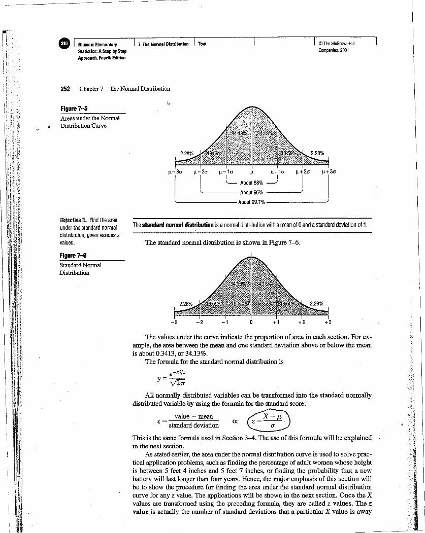
Figure 7-5Areas under the NormalDistribution Curve
7.TheNormel Distribution Text ©TheMcGraw-HiliCompenies. 2001
-t
J.l-30' J.l-20' J.l-10' J.l J.l+ 10' J.l+ 20' J.l+ 30'
II I
I'-- About 68% --l
About 95% }
About 99.7% }
value - meanZ = standard deviation
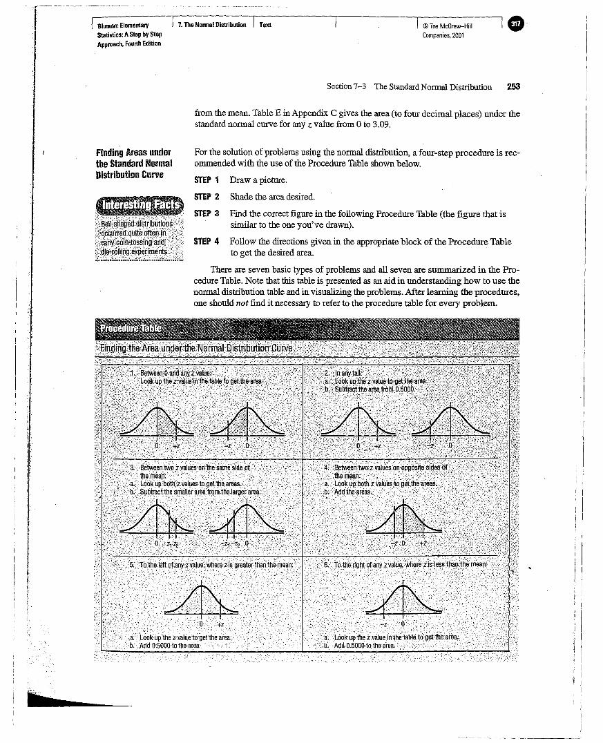
The standard normal distribution is shown in Figure 7-fJ.
The standard normal distribution is anormal distribution with amean of 0and astandard deviation of1.
All normally distributed variables can be transformed into the standard normallydistributed variable by using the formula for the standard score:
m@
The values wider the curve indicate the proportion of area in each section. For example, the area between the mean and one standard deviation above or below the meanis about 0.3413, or 34.13%.
The formula for the standard normal distribution is
This is the same formula used in Section 3-4. The use of this formula will be explainedin the next section.
As stated earlier, the area under the normal distribution curve is used to solve practical application problems, such as finding the percentage of adult women whose heightis between 5 feet 4 inches and 5 feet 7 inches, or finding the probability that a newbattery will last longer than four years. Hence, the major emphasis of this section willbe to show the procedure for finding the area under the standard normal distributioncurve for any z value. The applications will be shown in the next section. Once the Xvalues are transformed using the preceding formula, they are called z values. The zvalue is actually the number of standard deviations that a particular X value is away
l:lllj&~tiva3. Firid the areaunder the standard normaldistribution, given various zvalues.
Standard NormalDistribution
Figure 7-6
8luman: ElementaryStatistics: AStepbyStepApproach. Fourth Edition
7.TheNormal Distribution Text © The McGraw-HiliCompanies. 2001
Section7-3 The StandardNormal Distribution 253
Finding Areas underthe Standard NormalDistribution Curve
from the mean. Table E in Appendix C gives the area (to four decimal places) under thestandard normal curve for any z value from 0 to 3.09.
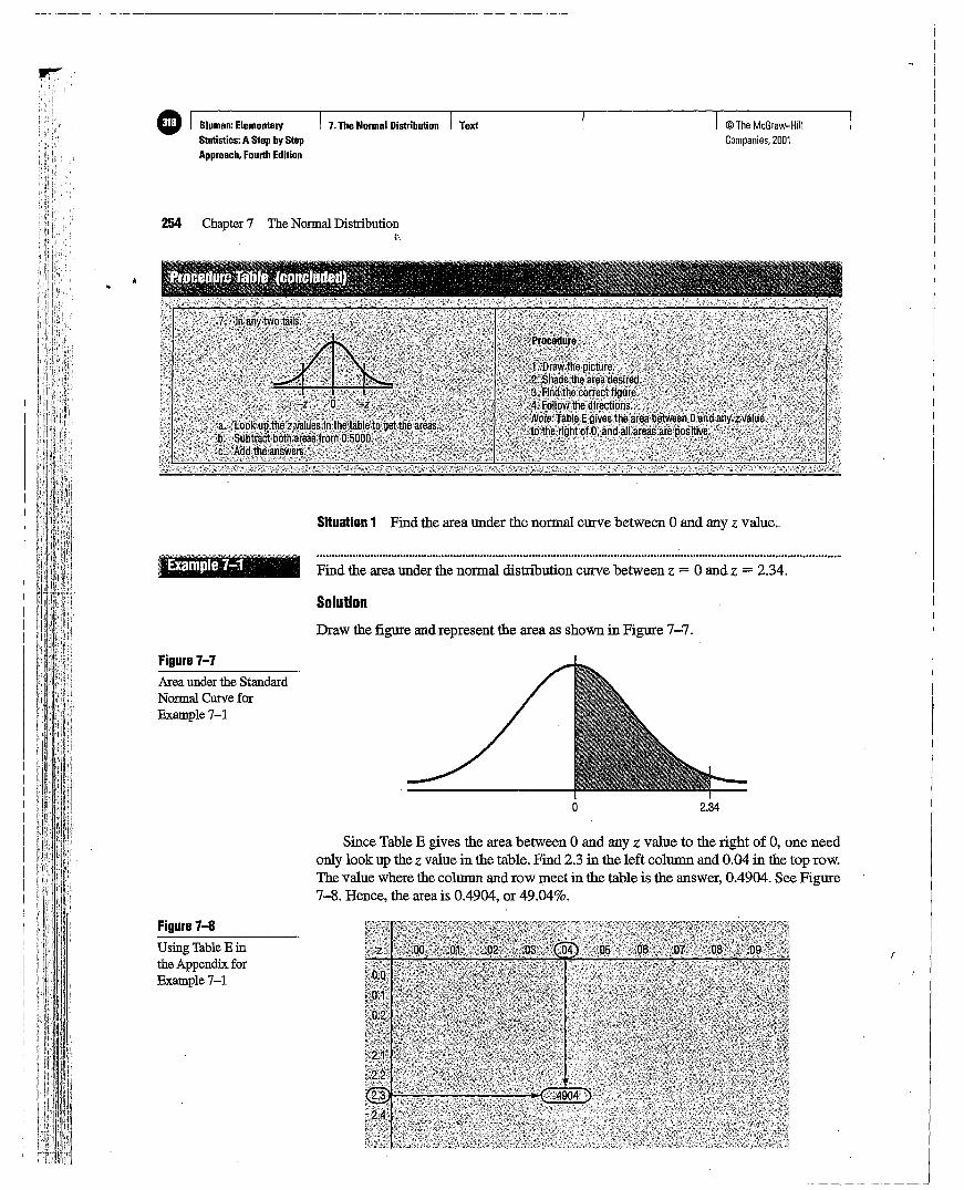
For the solution of problems using the normal distribution, a four-step procedure is recommended with the use of the Procedure Table shown below.
STEP 1 Draw a picture.
STEP 2 Shade the area desired.
STEP 3 Find the correct figure in the following Procedure Table (the figure that issimilar to the one you've drawn).
STEP 4 Follow the directions given in the appropriate block of the Procedure Tableto get the desired area.
There are seven basic types of problems and all seven are summarized in the Procedure Table. Note that this table is presented as an aid in understanding how to use thenormal distribution table and in visualizing the problems. After learning the procedures,one should not find it necessary to refer to the procedure table for every problem.
254 Chapter 7 The Normal Distributiont·,
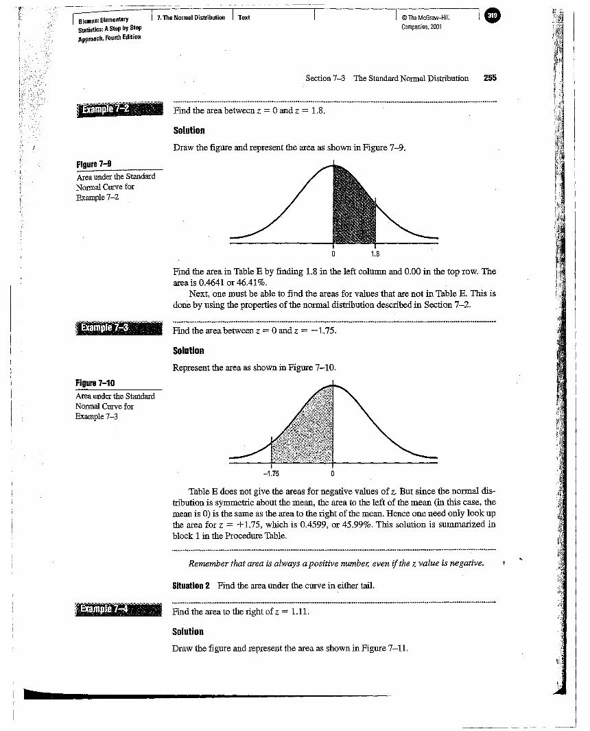
Find the area under the normal distribution curve between z = 0 and z = 2.34.
© The McGraw-HiliCompanies, 2001
Situation 1 Find the area under the normal curve between 0 and any z value;
, Example7-1 "" <
e I Bluman: Elementary I 7.TheNormal Distribution j TextStatistics: AStepbyStepApproach, Fourth Edition
..
Solution
Draw the figure and represent the area as shown in Figure 7-7.
Since Table E gives the area between 0 and any z value to the right of 0, one needonly look up the z value in the table. Find 2.3 in the left column and 0.04 in the top tow.The value where the column and row meet in the table is the answer, 0.4904. See Figure7-8. Hence, the area is 0.4904, or 49.04%.
figure 7-7Area under the StandardNormal Curve for
. Example 7-1
o 2.34
figure 7-8Using Table E inthe Appendix forExample 7-1
Solution
© The McGraw-HiliCompanies. 2001
Section 7-3 The Standard Normal Distribution 255
Draw the figure and represent the area as shown in Figure 7-9.
Find the area between z = 0 and z = 1.8.
7.TheNormal Distribution TextBluman: ElementaryStatistics: AStepbyStepApproach. Fourth Edition
Area under the StandardNormal Curve forExample 7-2
Figure 7-9
o 1.8
Find the area in Table E by finding 1.8 in the left column and 0.00 in the top row. Theareais 0.4641 or 46.41%.
Next, one must be able to find the areas for values that are not in Table E. This isdone by using the properties of the normal distribution described in Section 7-2.
EXample 7"-3 Find the area between z = 0 and z = -1.75.
Solution
Represent the area as shown in Figure 7-10.
Figure 7-10Area under the StandardNormal Curve forExample 7-3
-1.75 o
Table E does not give the areas for negative values of z, But since the normal distribution is symmetric about the mean, the area to the left of the mean (in this case, themean is 0) is the same as the area to the right of the mean. Hence one need only look upthe area for z = +1.75, which is 0.4599, or 45.99%. This solution is summarized inblock 1 in the Procedure Table.
Remember that area is always a positive number, even if the z value is negative.
Situation 2 Find the area under the curve in either tail.
mple7+4 Find the area to the right of z = 1.11.
Solution
Draw the figure and represent the area as shown in Figure 7-11.
b _
----- --~- - --~ --~----- -~-~-~----
e Bluman: ElementaryStatistics:AStepbyStepApproach, Fourth Edition
7.TheNormal Distribution Text © The McGraw-HiliCompanies. 2001
256 Chapter 7 The Normal Distribution
Figure 7-11Area under the Standard
• Normal Curve forExample 7-4
o 1.11
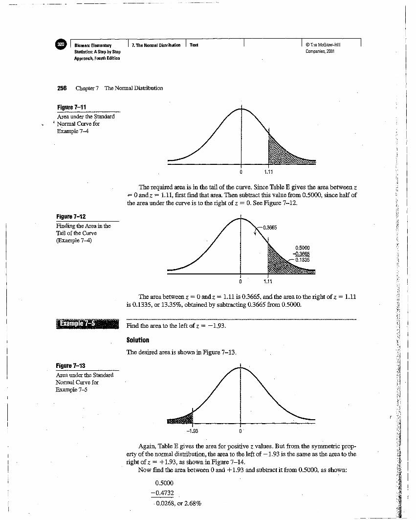
The required area is in the tail of the curve. Since Table E gives the area between z= 0 and z = 1.11,first fmd that area. Then subtract this value from 0.5000, since half ofthe area under the curve is to the right of z = O. See Figure 7-12.
Figure 7-12Finding the Area in theTail of the Curve(Example 7-4)
o 1.11
The areabetweenz = Oandz = 1.11 is 0.3665, and the area to the right ofz = 1.11is 0.1335, or 13.35%, obtained by subtracting 0.3665 from 0.5000.
Example 7+5 .
Figure 7-13Area under the StandardNormal Curve forExample 7-5
Find the area to the left of z = -1.93.
SolutionThe desired area is shown in Figure 7-13.
-1.93 o
Again, Table E gives the area for positive zvalues. But from the symmetric property of the normal distribution, the area to the left of -1.93 is the same as the area to theright of z = +1.93, as shown in Figure 7-14.
Now find the area between 0 and + 1.93 and subtract it from 0.5000, as shown:
0.5000
-0.4732
.0.0268, or 2.68%

This procedure was summarized in block 2 of the Procedure Table.
Find the area between z = 2.00 and z = 2.47.
IIII
IJI''IIII''II,II
III,I
'I
:!I
257
+1.93
©The McGraw-Hili, Companies, 2001
o
o
Section 7-3 The Standard Nanna! Distribution
-1.93
Text
Situation 3 Find the area under the curve between any two zvalues on the same side ofthe mean.
7.TheNormal DistributionBluman: ElementaryStatistics: AStepbyStepApproech, Fourth Edition
Figure 7-14Comparison of Areas tothe Right of +1.93 and tothe Left of -1.93(Example 7-5)
ample 7
Solution
Figure 7-15
Area under the Curve forExample 7-6
The desired area is shown in Figure 7-15.
Figure 7-16Finding the Areaunder the Curve forExample 7-6
o 2.00 2.47
For this situation, look up the area from z = 0 to Z = 2.47 and the area from z = 0to Z = 2.00. Then subtract the two areas, as shown in Figure 7-16.
~-- 0.4932--~
! 'k_'
o 2.00 2.47
---------
Solution
Find the area between z = -2.48 and z = -0.83.
© The McGrew-HiliCompanies. 2001
1.68
o
o
-0.83
-1.37
Text
-2.48
7.TheNormal Distribution
Solution
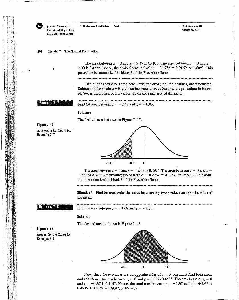
The desired area is shown in Figure 7-17.
The area between z = 0 and z = 2.47 is 0.4932. The area between z = 0 and z =2.00 is 0.4772. Hence, the desired area is 0.4932 - 0.4772 = 0.0160, or 1.60%. Thisprocedure is summarized in block 3 of the Procedure Table.
Two things should be noted here. First, the areas, not the z values, are subtracted.Subtracting the z values will yield an incorrect answer. Second, the procedure in Example 7-6 is used when both z values are on the same side of the mean.
Now, since the two areas are on opposite sides of z = 0, one must find both areasand add them. The area between z = 0 and z = 1.68 is 0.4535. The area between z = 0and z = -1.37 is 0.4147. Hence, the total area between z = -1.37 and z -= +1.68 is0.4535 + 0.4147 = 0.8682, or 86.82%.
The area between z = 0 and z = -2.48 is 0.4934. The area between z = 0 and z =-0.83 is 0.2967. Subtracting yields 0.4934 - 0.2967 = 0.1967, or 19.67%. This solution is summarized in block 3 of the Procedure Table.
The desired area is shown in Figure 7-18.
Situation 4 Find the area under the curve between any two z values on opposite sides ofthe mean.
Find the area between z = + 1.68 and z = -1.37.
8luman: ElamentaryStatistics:AStep bV StepApproach. Fourth Edition
258 Chapter 7 The Normal Distribution
"
e Example 7~7
"Examp e7-+8 "
Area under the Curve forExample 7-7
Figure 7-17
Area under the CurveforExample 7-8
Figure 7-18

The desired area is shown in Figure 7-19.
Solution
'•...:\'I
IiIiIII!
\1
© The McGrew-HiliCompanies. 2001
1.99o
Section 7-3 The Standard Normal Distribution 259
This type of problem is summarized in block 4 of the Procedure Table.
Situation 5 Find the area under the curve to the left of any z value, where z is greaterthan the mean.
Find the area to the left of z = 1.99.
Since Table E gives only the area between z = 0 and z = 1.99, one must add 0.5000to the table area, since 0.5000 (half) of the total area lies to the left of z = O. The areabetweenz = 0 andz = 1.99 is 0.4767, and the total area is 0.4767 + 0.5000 = 0.9767,or 97.67%.
This solution is summarized in block 5 of the Procedure Table.
7.TheNormal Distribution Text
Example 7--9 '
Bluman: ElementaryStatistics: AStepbyStepApproach, fourth Edition
Figure 7-19Area under the Curve forExample 7-9
\
EXample 7-10 '
Figure 7-20Area under the Curve forExample 7-10
The same procedure is used when the z value is to the left of the mean, as shown inthe next example.
Situation 6 Find the area under the curve to the right of any zvalue, where z is less thanthe mean.
Find the area to the right of z = -1.16.
Solution
The desired area is shown in Figure 7-20.
-1.16 0
The area betweenz = 0 andz = -l.16is 0.3770. Hence, the total area is 0.3770 +0.5000 = 0.8770, or 87.70%.
;.This type of problem is summarized in block 6 of the Procedure Table.
© The McGraw-HiliCompanies. 2001
2.43o-3.01
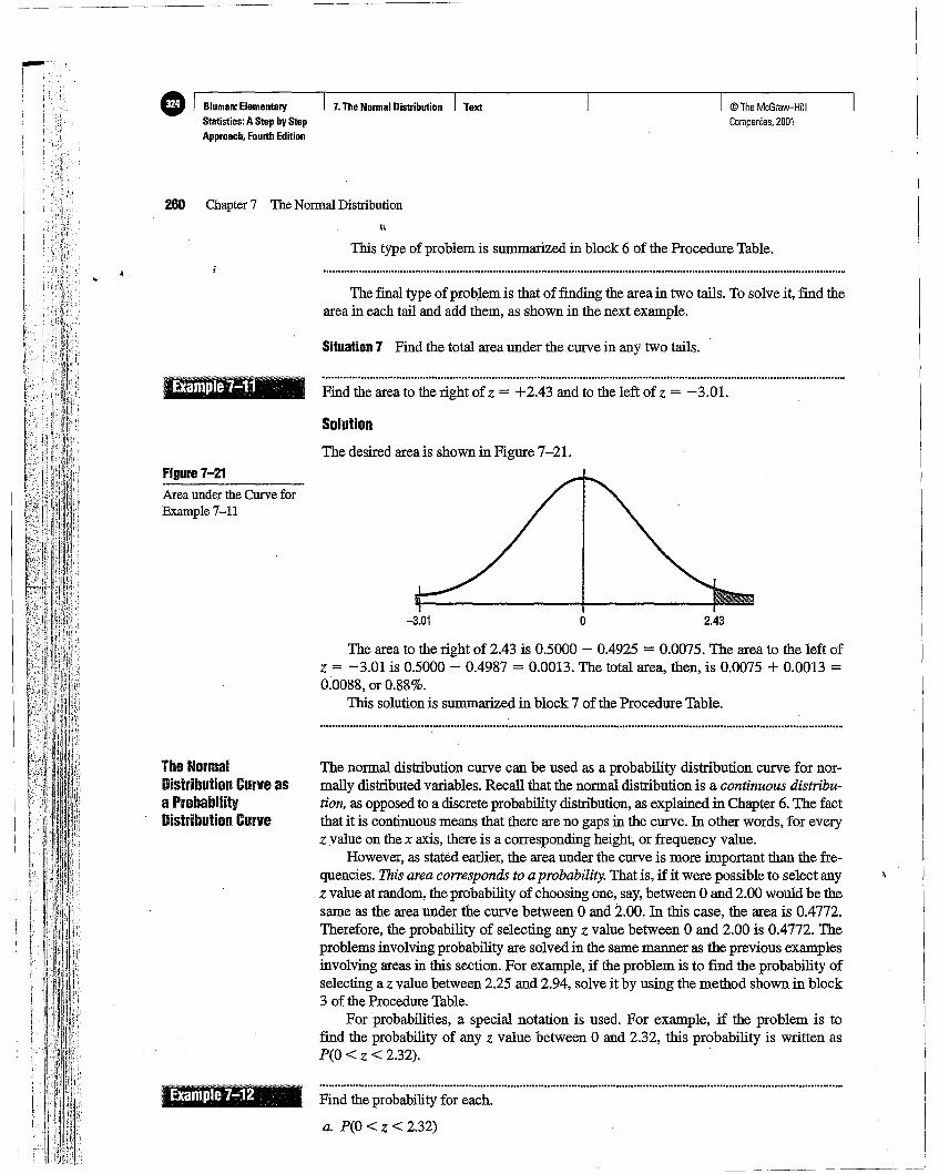
The desired area is shown in Figure 7-21.
Find the area to the right of z = +2.43 and to the left of z = -3.01.
Find the probability for each.
a. P(O < z < 2.32)
Situation 7 Find the total area under the curve in any two tails.
The area to the right of 2.43 is 0.5000 - 0.4925 = 0.0075. The area to the left ofz = -3.01 is 0.5000 - 0.4987 = 0.0013. The total area, then, is 0.0075 + 0.0013 =0:0088, or 0.88%.
This solntion is summarized in block 7 of the Procedure Table.
Solution
The normal distribution curve can be used as a probability distribution curve for normally distributed variables. Recall that the normal distribution is a continuous distribution, as opposed to a discrete probability distribution, as explained in Chapter 6. The factthat it is continuous means that there are no gaps in the curve. In other words, for everyzvalue on the x axis, there is a corresponding height, or frequency value.
However, as stated earlier, the area under the curve is more important than the frequencies. This area corresponds to a probability. That is, if it were possible to select anyz value at random, the probability of choosing one, say, between 0 and 2.00 would be thesame as the area under the curve between 0 and 2.00. In this case, the area is 0.4772.Therefore, the probability of selecting any z value between 0 and 2.00 is 0.4772. Theproblems involving probability are solved in the same manner as the previous examplesinvolving areas in this section. For example, if the problem is to fmd the probability ofselecting az value between 2.25 and 2.94, solve it by using the method shown in block3 of the Procedure Table.
For probabilities, a special notation is used. For example, if the problem is tofind the probability of any z value between 0 and 2.32, this probability is written asP(O < z < 2.32).
The final type of problem is that of finding the area in two tails. To solve it, find thearea in each tail and add them, as shown in the next example.
Figure 7-21
; EXample 7-1
Area under the Curve forExample 7-11
Example 7-12
The NormalDistribution Curve asaProbabilityDistribution Curve
260 Chapter7 The Normal Distribution
e I Bluman: Elementary _ I 7.TheNormal Distribution I TextStatistics: A Step byStepApproach. Fourth Edition
..
---,!
II
IiI
IV
2.32
I © The McGraw-HiliCompanies. 2001
1.91
1.65
o
r
Section 7-3 The Standard Normal Distribution 261
o
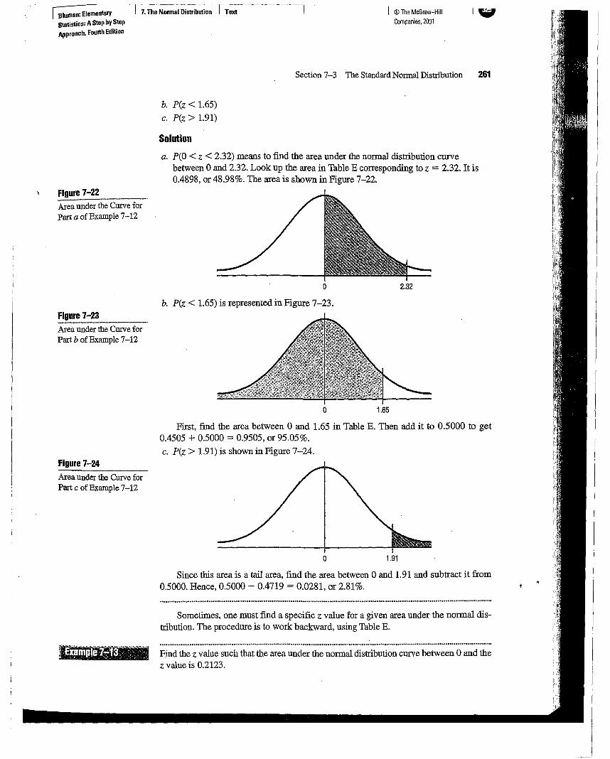
ob. P(z < 1.65) is represented in Figure 7-23.
Sometimes, one must fmd a specific z value for a given area under the normal distribution. The procedure is to work backward, using Table E.
Since this area is a tail area, find the area between 0 and 1.91 and subtract it from0.5000. Hence, 0.5000 - 0.4719 = 0.0281, or 2.81%.
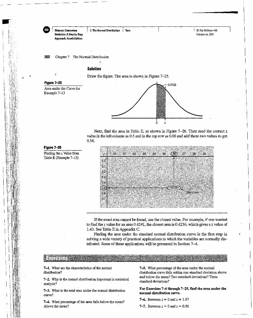
Find the zvalue such that the area under the normal distribution curve between 0 and thez value is 0.2123.
First, find the area between 0 and 1.65 in Table E. Then add it to 0.5000 to get0.4505 + 0.5000 = 0.9505, or 95.05%.
c. P(z> 1.91) is shown in Figure 7-24.
b. P(Z < 1.65)
c. P(z > 1.91)
Solution
a. P(O < z < 2.32) means to find the area under the normal distribution curvebetween 0 and 2.32. Look up the area in Table E corresponding to z = 2.32. It is0.4898, or 48.98%. The area is shown in Figure 7-22.
Area under the Curve forPart c of Example 7-12
Figure 7-24
Area under the Curve forPart a of Example 7-12
Area under the Curve forPart b of Example 7-12
Figure 7-22
Figure 7-23
f;luman: Elementary ~.-r 7.~N;;r;;;al m~rib-~ion IT~~--SUrtistics: AStepby StepApproach. Fourth Edition
© The McGraw-HiliCompanies. 2001
7-5. What percentage of the area under the normaldistribution curve falls within one standard deviation aboveand below the mean? Two standard deviations? Threestandard deviations?
For Exercises 7-6 through 7-25, find the area under thenormal distribution curve.
7-6. Between z = 0 and z = 1.97
7-7. Between z = 0 and z = 0.56
o z
Draw the figure. The area is shown in Figure 7-25.
Solution,.
262 Chapter 7 The Normal Distributiont,
Figure 7-25
Area under the Curve forExample 7-13
Next, find the area in Table E, as shown in Figure 7-26. Then read the correct Z
value in the left column as 0.5 and in the top row as 0.06 and add these two values to get0.56.
Figure 7-26
If the exact area cannot be found, use the closest value. For example, ifone wantedto find the zvalue for an area 0.4241, the closest area is 0.4236, which gives a Z value of1.43. See Table E in Appendix C.
Finding the area under the standard normal distribution curve is the first step insolving a wide variety of practical applications in which the variables are normally distributed. Some of these applications will be presented in Section 7~.
Finding the z ValuefromTable E (Example 7-13)
7-1. What are the characteristics of the normaldistribution?
7-2. Why is the normal distribution important in statisticalanalysis?
7-3. What is the total area under the normal distributioncurve?
7-4•. What percentage of the area falls below the mean?Above the mean?
e I Bluman: Elementary I 7.TheNormal Distribution I TextStatistics: A Step byStepApproach. Fourth Edition
0.0239
z
z
z
o
o
o
o
o
o
z
z
z
© The McGraw-HiliCompanies. 2001
Section 7-3 The Standard Normal Distribution 263
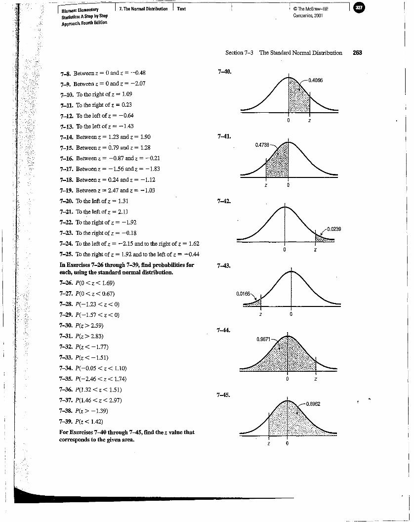
7-41.
7-40.
7-42.
7-43.
7-44.
7-45.
7.TheNormal Distribution TextBluman: ElementaryStatistics: AStepbyStepApproach, Fourth Edition
7-S. Between z = 0 and z = -0.48
7-9. Between z = 0 and z = -2.07
7-10. To the right of z = 1.09
7-U. To the right of z = 0.23
7-12. To the left of z = -0.64
7-13. To the left of z = -1.43
7-14. Between z = 1.23 and z = 1.90
7-15. Between z = 0.79 and z = 1.28
7-16. Between z = -0.87 and z = -0.21
7-17. Between z = -1.56 and z = -1.83
7-18. Between z = 0.24 and z = -1.12
7-19. Between z = 2.47 and z = -1.03
7-20. To the left of z = 1.31
7-21. To the left of z = 2.11
7-22. To the right of z = -1.92
7-23. To the right of z = -0.18
7-24. To the left of z = -2.15 and to the right of z = 1.62
7-25. To the right of z = 1.92and to the left of z = -0.44
In Exercises 7-26 through 7-39, find probabilities foreach, using the standard normal distribution.
7-26. P(O < z < 1.69)
7-27. P(O < z < 0.67)
7-28. P(-1.23 < z < 0)
7-29. P( -1.57 < z < 0)
7-30. P(z > 2.59)
7-31. P(z > 2.83)
7-32. P(z < -1.77)
7-33. P(z < -1.51)
7-34. P(-0.05 < z < 1.10)
7-35. P(-2.46 < z < 1.74)
7-36. P(1.32< z < 1.51)
7-37. P(1.46< z < 2.97)
7-38. P(z > -1.39)
7-39. P(z < 1.42)
For Exercises 7-40 through 7-45, find the z value thatcorresponds to the given area.
II
~------------
Bluman: ElementaryStatistics:AStep bV StepApproach, Fourth Edition
7.TheNormal Distribution TeXl © The McGraw-HiliCompanies. 2001
264 Chapter 7 The Normal Distribution
This is the same formula presented in Section 3-4. This formula transforms the valuesof the variable into standard units or z values. Once the variable is transformed, then theProcedure Table and Table E in Appendix C can be used to solve problems.
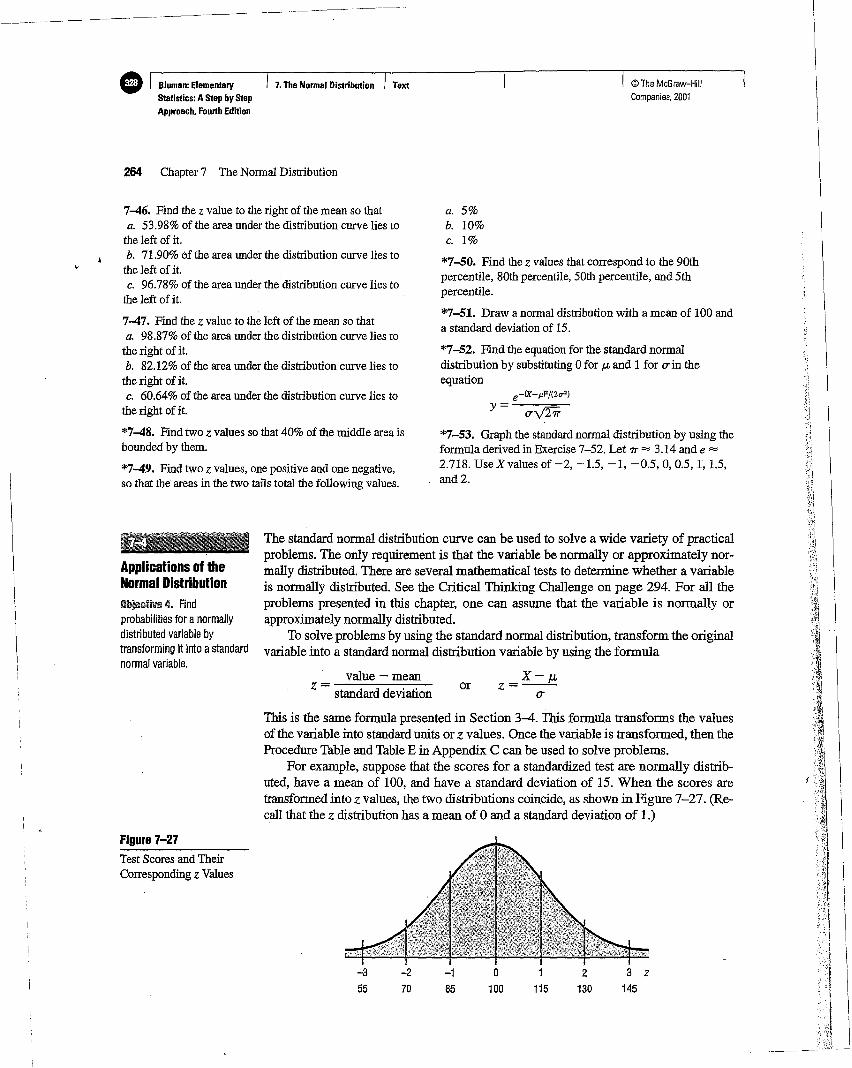
For example, suppose that the scores for a standardized test are normally distributed, have a mean of 100, and have a standard deviation of 15. When the scores aretransformed into z values, the two distributions coincide, as shown in Figure 7-27. (Recall that the z distribution has a mean of aand a standard deviation of 1.)
3 z145
2
1301
115
x-p.,z=-0-
o100
or
-1
85
a.5%b. 10%c. 1%
*7-50. Find the z values that correspond to the 90thpercentile, 80th percentile, 50th percentile, and 5thpercentile.
*7-51. Draw a normal distribution with a mean of 100 anda standard deviation of 15.
*7-52. Find the equation for the standard normaldistribution by substituting 0 for J.L and 1 for o-in theequation
e-rx- p.'P/(2u 2 )
y = 0-V27i-
*7-53. Graph the standard normal distribution by using theformula derived in Exercise 7-52. Let 7T = 3.14 and e =2.718. Use X values of -2, -1.5, -1, -0.5,0,0.5,1,1.5,and 2.
-2
70
-355
value - meanZ = standard deviation
The standard normal distribution curve can be used to solve a wide variety of practicalproblems. The only requirement is that the variable be normally or approximately normally distributed. There are several mathematical tests to determine whether a variableis normally distributed. See the Critical Thinking Challenge on page 294. For all theproblems presented in this chapter, one can assume that the variable is normally orapproximately normally distributed.
To solve problems by using the standard normal distribution, transform the originalvariable into a standard normal distribution variable by using the formula
7-46. Find the z value to the right of the mean so thata. 53.98% of the area under the distribution curve lies to
the left of it.b. 71.90% ef the area under the distribution curve lies to
the left of it.c. 96.78% of the area under the distribution curve lies to
the left of it.
7-47. Find the z value to the left of the mean so thata. 98.87% of the area under the distribution curve lies to
the right of it.b. 82.12% of the area under the distribution curve lies to
the right of it.c. 60.64% of the area under the distribution curve lies to
the right of it.
*7-48. Find two z values so that 40% of the middle area isbounded by them.
*7-49. Find two z values, one positive and one negative,so that the areas in the two tails total the following values.
Applications of theNormal Distribution~!)jet\tille 4. Findprobabilities foranormallydistributed variable bytransforming it into astandardnormal variable.
Test Scores and TheirCorresponding z Values
Figure 7-27
100 112
Solution
© The McGraw-HiliCompanies. 2001
Section 7-4 Applications of the Normal Distribution 265
To solve the application problems in this section, transform the values of the variable into z values and then use the Procedure Table and Table E, as shown in the nextexamples.
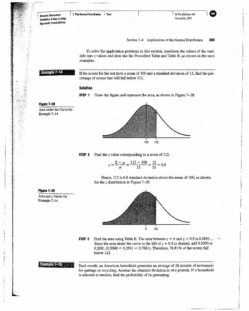
STEP 1 Draw the figure and represent the area, as shown in Figure 7-28.
If the scores for the test have a mean of 100 and a standard deviation of 15, find the percentage of scores that will fall below 112.
7.TheNonnel Distribution Text
Example 7-14
Blumen: ElementaryStatistics: AStep byStepApproach, Fourth Edition
Area under the Curve forExample 7-14
Figure 7-28
STEP 2 Find the zvalue corresponding to a score of 112.
z =X - JL = 112 - 100 = 12 = 0 8(T 15 15'
Hence, 112 is 0.8 standard deviation above the mean of 100, as shownfor the z distribution in Figure 7-29.
Figure 7-29
Area and z Values forExample 7-14
o 0.8
STEP 3 Find the area using Table E. The area between z = 0 and z =:= 0.8 is 0.2881. t
Since the area under the curve to the left of z = 0.8 is desired, add 0.5000 to0.2881 (0.5000 + 0.2881 = 0.7881). Therefore, 78.81% of the scores fallbelow 112.
Each month, an American household generates an average of 28 pounds of newspaperfor garbage or recycling. Assume the standard deviation is two pounds. If a householdis selected at random, find the probability of its generating
•--"-f:
I"II
i
8luman:ElementaryStatistics:AStepby StepApproach. Fourth Edition
7.TheNormal Distribution Text © The McGraw-HiliCompanies. 2001
266 Chapter 7 The Normal Distribution
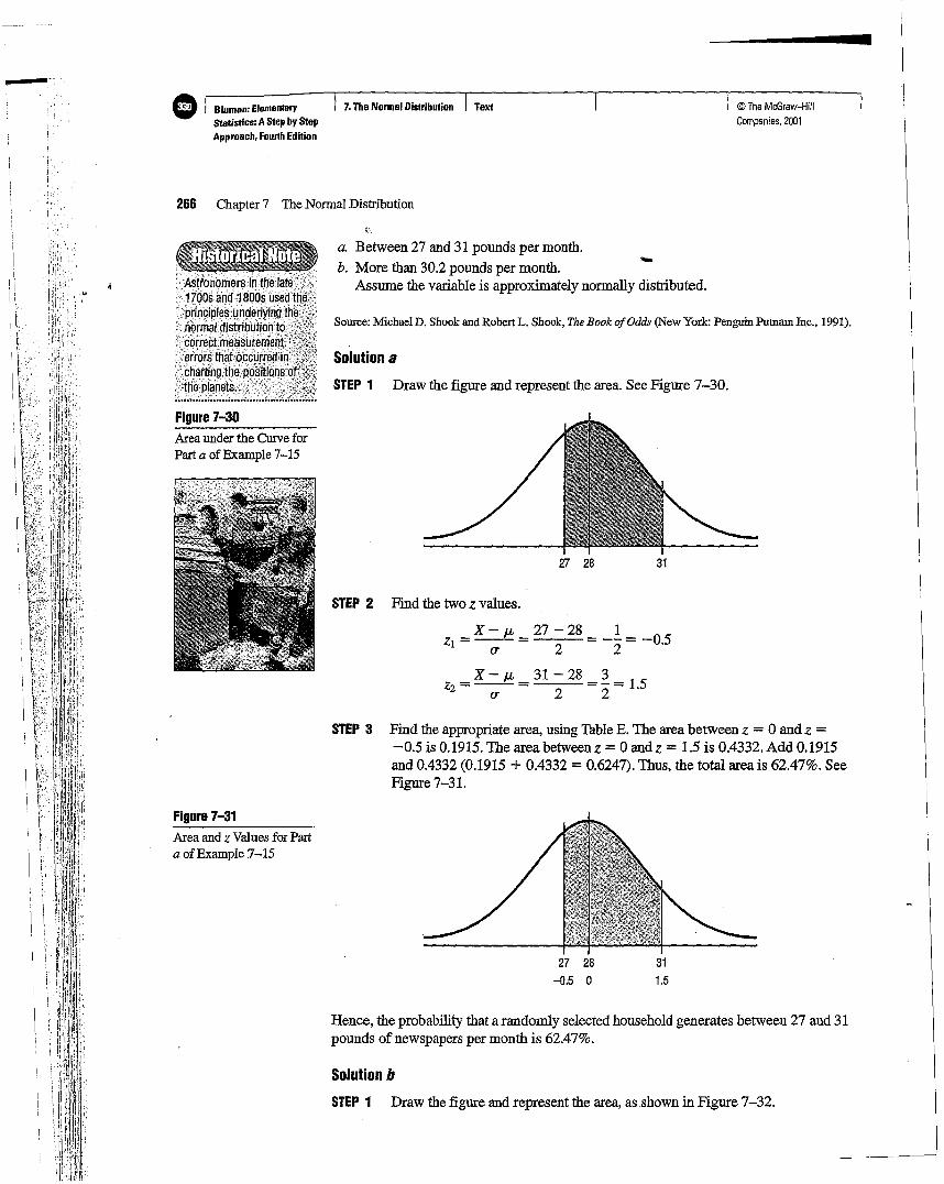
a. Between 27 and 31 pounds per month.
b. More than 30.2 pounds per month.Assume the variable is approximately normally distributed.
Solution aSTEP 1 Draw the figure and represent the area. See Figure 7-30.
27 28 31-0.5 0 1.5
27 28 31
Source:MichaelD. Shookand RobertL. Shook,TheBook ofOdds (New York:Penguin Putnam Inc., 1991).
STEP 3 Find the appropriate area, using Table E. The area between Z = 0 and Z =-0.5 is 0.1915. The area between z = 0 and z = 1.5 is 0.4332. Add 0.1915and 0.4332 (0.1915 + 0.4332 = 0.6247). Thus, the total area is 62.47%. SeeFigure 7-31.
STEP 2 Find the two Z values.
X- JL 27 - 28 1Zl = -(F- = 2 = -:2 = -0.5
X - JL 31 - 28 3Zz = -(F- = 2 = :2 = 1.5
STEP 1 Draw the figure and represent the area, as shown in Figure 7-32.
Hence, the probability that a randomly selected household generates between 27 and 31pounds of newspapers per month is 62.47%.
Solution b
:.principie'ormal
Orrec!'~t
,chatliJ;g.i;ftie'pllme
Figure 7-30Area under the Curve forPart a of Example 7-15
Area and zValues for Parta of Example 7-15
Figure 7-31
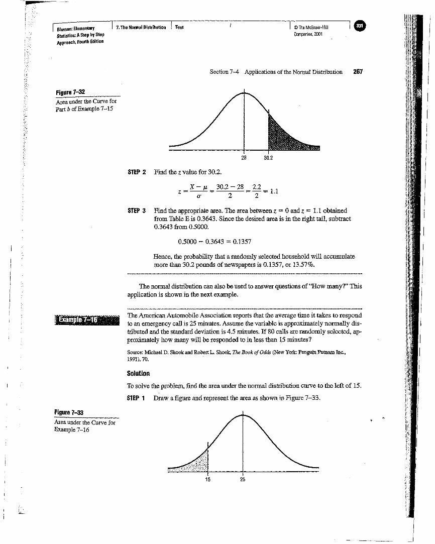
28 30.2
© The McGraw-HiliCompanies. 2001
Section 7-4 Applications of the Normal Distribution 267
15 25
STEP 3 Find the appropriate area. The area between z = 0 and z = 1.1 obtainedfrom Table E is 0.3643. Since the desired area is in the right tail, subtract0.3643 from 0.5000.
z =X - I.J. = 30.2 - 28 = 2.2 = 1.1a' 2· 2
STEP 2 Find the z value for 30.2.
0.5000 - 0.3643 = 0.1357
Hence, the probability that a randomly selected household will accumulatemore than 30.2 pounds ofnewspapers is 0.1357, or 13.57%.
The normal distribution can also be used to answer questions of "How many?" Thisapplication is shown in the next example.
The American Automobile Association reports that the average time it takes to respondto an emergency call is 25 minutes. Assume the variable is approximately normally distributed and the standard deviation is 4.5 minutes. If 80 calls are randomly selected, approximately how many will be responded to in less than 15 minutes?
To solve the problem, find the area under the normal distribution curve to the left of 15.
STEP 1 Draw a figure and represent the area as shown in Figure 7-33.
Source: MichaelD. Shookand Robert L. Shook,The Book of Odds (NewYork: PenguinPutnam Inc.,1991),70.
Solution
7.TheNormal Distribution TextBluman: ElementaryStatistics: AStepbyStepApproach. Fourth Edition
Area under the Curve forPart b of Example 7-15
Figure 7-32
Area under the Curve forExample 7-16
Figure 7-33
STEP 3 Find the appropriate area. The area obtained from Table E is 0.4868, whichcorresponds to the area between z = 0 and z = -2.22 (Use +2.22.)
STEP 4 Subtract 0.4868 from 0.5000 to get 0.0132.
STEP 5 To find how many calls will be made in less than 15 minutes, multiply thesample size (80) by the area (0.0132) to get 1.056. Hence, 1.056, orapproximately one, call will be responded to in under 15 minutes.
268 Chapter 7 The Normal Distributiont,
© The McGraw-Hili.Companies. 2001
STEP 2 Find the zvalue for 15.
z = X - f.L = 15 - 25 = -2.22(T 4.5
The normal distribution can also be used to find specific data values for given percentages. This application is shown in the next example.
Note: For problems using percentages, be sure to change the percentage to a decimal before multiplying. Also, round the answer to the nearest whole number, since it isnot possible to have 1.056 calls.
200 X
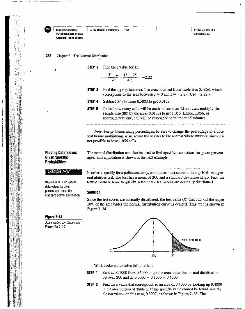
Since the test scores are normally distributed, the test value (X) that cuts off the upper10% of the area under the normal distribution curve is desired. This area is shown inFigure 7-34.
Solution
Work backward to solve this problem
STEP 1 Subtract 0.1000 from 0.5000 to get the area under the normal distributionbetween 200 and X: 0.5000 - 0.1000 = 0.4000.
STEP 2 Find the z value that corresponds to an area of 0.4000 by looking up 0.4000in the area portion of Table E. If the specific value cannot be found, use theclosest value-in this case, 0.3997, as shown in Figure 7-35. The
In order to qualify for a police academy, candidates must score in the top 10% on a general abilities test. The test has a mean of 200 and a standard deviation of 20. Find thelowest possible score to qualify. Assume the test scores are normally distributed.
;.
Example 7-17
~lljllil::tlve 5. Find specificdata values forgivenpercentag as using thestandard normal distribution.
finding Data ValuesGiven SpecificProbabilities
Area under the CurveforExample 7-17
Figure 7-34
e I 8luman: Elementary I 7.TheNormal Distribution I TextStatistics: AStepbyStepApproach, Fourth Edition

-------------- -- - - --- -- ----
© The McGraw-HiliCompanies. 2001
Multiply both sides by 0'.
Add JL to both sides.
Exchange both sides of the equation.
Section 7-4 Applications of the Normal Distribution 269
z·O'=X-JL
z'u+JL=X
X=z'u+JL
corresponding Z value is 1.28. (If the area falls exactly halfway between twoz values, use the larger of the two z values. For example, the area 0.4500falls halfway between 0.4495 and 0.4505. In this case use 1.65 rather than1.64 for the z value.)
A score of 226 should be used as a cutoff. Anybody scoring 226 or higher qualifies.
STEP 3 Substitute in the formula z = (X - JL)/0' and solve for X.
1.28 =X ~goo
(1.28)(20) + 200 = X
25.60 + 200 = X
225.60 =X
226 =X
Instead of using the formula shown in Step 3 one can use the formula X = z . 0' + JL.This is obtained by solving
z = (X - JL) for X0'
as shown.
7.The Normal Distribution TextBluman: ElementaryStatistics: AStep byStepApproach, Fourth Edition
Figure 7-35Finding the zValue fromTableE (Example 7-17)
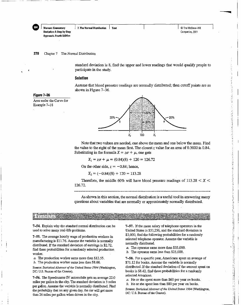
For a medical study, a researcher wishes to select people in the middle 60% of the population based on blood pressure. If the mean systolic blood pressure is 120 and the
b _
Solution
© The McGraw-HiliCompanies. 2001
7-57. If the mean salary of telephone operators in theUnited States is $31,256, and the standard deviation is$3,000, find the following probabilities for a randomlyselected telephone operator. Assume the variable isnormally distributed.a. The operator earns more than $35,000.b. The operator earns less than $25,000.
7-58. For a specific year, Americans spent an average of$71.12 for books. Assume the variable is normallydistributed. If the standard deviation of the amount spent onbooks is $8.42, find these probabilities for a randomlyselected American.a. He or she spent more than $60 per year on books.b. He or she spent less than $80 per year on books.
Source: Statistical Abstract ofthe United States 1994 (Washington,DC: U.S. Bureau of the Census).
7.TheNormal Distribution Text
X2 = (-0.84)(8) + 120 = 113.28
Therefore, the middle 60% will have blood pressure readings of 113.28 < X <126.72.
On the other side, z = -0.84; hence,
Note that two values are needed, one above the mean and one below the mean. Findthe value to the right of the mean first. The closest z value for an area of 0.3000 is 0.84.Substituting in the formula X = za + p" one gets
Xl = zo:+ p, = (0.84)(8) + 120 = 126.72
Area under the Curve forExample 7-18
Figure 7-36
Assume that blood pressure readings are normally distributed; then cutoff points are asshown in Figure 7-36.
As shown in this section, the normal distribution is a useful tool in answering manyquestions about variables that are normally or approximately normally distributed.
standard deviation is 8, find the upper and lower readings that would qualify people toparticipate in the study.
7-54. Explain why the standard normal distribution can beused to solve many real-life problems.
7-55. The average hourly wage of production workers inmanufacturing is $11.76. Assume the variable is normallydistributed. If the standard deviation of earnings is $2.72,find these probabilities for a randomly selected productionworker.a. The production worker earns more than $12.55.b. The production worker earns less than $8.00.
Source: Statistical Abstract ofthe United States 1994 (Washington,DC: U.S. Bureau of the Census).
7-56. The Speedmaster N automobile gets an average 22.0miles per gallon in the city. The standard deviation is 3 milesper gallon. Assume the variable is normally distributed. Findthe probability that on any given day, the car will get morethan 26 miles per gallon when driven in the city.
270 Chapter 7 The Normal Distribution
e 8luman: ElementaryStatistics: AStepbyStepApproach. Fourth Edition
7-65. The average waiting time for a drive-in window at alocal bank is 9.2 minutes, with a standard deviation of 2.6minutes. When a customer arrives at the bank, find the
7-64. The average amount of rain per year in SouthSummerville is 49 inches. The standard deviation is5.6 inches. Find the probability that next year SouthSummerville will receive the following amount of rain.Assume the variable is normally distributed.a. At most 51 inches of rainb. At least 58 inches of rain
7-62. The average time a visitor spends at the Renzie ParkArt Exhibit is 62 minutes. The standard deviation is 12minutes. If a visitor is selected at random, find theprobability that he or she will spend the following amountof time at the exhibit. Assume the variable is normallydistributed.a. At least 82 minutesb. At most 50 minutes
7-63. The average time for a courier to travel fromPittsburgh to Harrisburg is 200 minutes, and the standarddeviation is 10 minutes. If one of these trips is selected atrandom, find the probability that the courier will have thefollowing travel time. Assume the variable is normallydistributed.a. At least 180 minutesb. At most 205 minutes
..
©TheMcGraw-HiliCompanies, 2001
probability that the customer will have to wait the followingamount of time. Assume the variable is normally distributed.a. Between 5 and 10 minutesb. Less than 6 minutes or more than 9 minutes
7-66. The average time it takes college freshmen tocomplete the Mason Basic Reasoning Test is 24.6 minutes.The standard deviation is 5.8 minutes. Find theseprobabilities. Assume the variable is normally distributed.a. It will take a student between 15 and 30 minutes to
complete the test.b. It will take a student less than 18 minutes or more than
28 minutes to complete the test. .
7-67. A brisk walk at 4 miles per hour burns an average of300 calories per hour. If the standard deviation of thedistribution is 8 calories, find the probability that a personwho walks one hour at the rate of 4 miles per hour willburn the following calories. Assume the variable isnormally distributed.a. More than 280 caloriesb. Less than 293 caloriesc. Between 285 and 320 calories
7-68. During September, the average temperature ofLaurel Lake is 64.2° and the standard deviation is 3.2°.Assume the variable is normally distributed. For arandomly selected day, find the probability that thetemperature will be as follows:a. Above62°b. Below 67°c. Between 65° and 68°
7-69. If the systolic blood pressure for a certain group ofobese people has a mean of 132 anda standard deviation of8, find the probability that a randomly selected obeseperson will have the following blood pressure. Assume thevariable is normally distributed.a. Above 130b. Below 140c. Between 131 and 136
7-70. In order to qualify for letter sorting, applicants aregiven a speed-reading test. The scores are normallydistributed, with a mean of 80 and a standard deviation of8. If only the top 15% of the applicants are selected, findthe cutoff score.
7-71. The scores on a test have a mean of 100 and astandard deviation of 15. If a personnel manager wishes toselect from the top 75% of applicants who take the test,find the cutoff score. Assume the variable is normallydistributed.
7-72. For an educational study, a volunteer must place inthe middle 50% on a test. If the mean for the population is100 and the standard deviation is 15, find the two limits(upper and lower) for the scores that would enable a
Section 7-4 Applications of the Normal Distribution 271
7.TheNormal Distribution TextBluman: ElementarySlatistics: ASlepbySlapApproach, Fourth Edition
7-59. A survey found that people keep their television setsan average of 4.8 years. The standard deviation is 0.89 year.If a person decides to buy a new TV set, fmd the probabilitythat he or she has owned the old set for the followingamount of time. Assume the variable is normally distributed.a. Less than 2.5 yearsb. Between 3 and 4 yearsc. More than 4.2 years
7-60. The average age of CEOs is 56 years. Assume thevariable is normally distributed. If the standard deviation isfour years, find the probability that the age of a randomlyselected CEO will be in the following range.a. Between 53 and 59 years oldb. Between 58 and 63 years oldc. Between 50 and 55 years old
Source: MichaelD. ShookandRobertL. Shook,The Book of Odds(New York: Penguin PutnamInc., 1991),49.
7-61. The average life of a brand of automobile tires is30,000 miles, with a standard deviation of 2,000 miles. If atire is selected and tested, find the probability that it willhave the following lifetime. Assume the variable isnormally distributed.a. Between 25,000 and 28,000 milesb. Between 27,000 and 32,000 milesc. Between 31,500 and 33,500 miles
272 Chapter 7 The Normal Distribution
volunteer to participate in the study. Assume the variable isnormally distributed.
7-73. A contractor decided to build homes that willinclude the middle 80% of the market. If the average size(in square feet) of homes built is 1,810, find the maximumand minimum sizes of the homes the contractor shouldbuild. Assume that the standard deviation is 92 square feetand the variable is normally distributed.
Source: Michael D. Shook andRobertL. Shook, The Book ofOdds(New York:Penguin PutnamInc., 1991), 15.
7-74. If the average price of a new home is $145,500, findthe maximum and minimum prices of the houses acontractor will build to include the middle 80% of themarket. Assume that the standard deviation of prices is$1,500 and the variable is normally distributed.
Source: Michael D. Shook andRobertL. Shook, TheBook ofOdds(New York:Penguin PutnamInc., 1991), 15.
7-75. An athletic association wants to sponsor a footrace.The average time it takes to run the course is 58.6 minutes,with a standard deviation of 4.3 minutes. If the associationdecides to award certificates to the fastest 20% of theracers, what should the cutoff time be? Assume the variableis normally distributed.
7-76. In order to help students improve their reading, aschool district decides to implement a reading program. Itis to be administered to the bottom 5% of the students inthe district, based on the scores on a reading achievementexam. If the average score for the students in the district is122.6, find the cutoff score that will make a student eligiblefor the program. The standard deviation is 18. Assume thevariable is normally distributed.
7-77. An automobile dealer finds that the average price ofa previously owned vehicle is $8,256. He decides to sellcars that will appeal to the middle 60% of the market interms of price. Find the maximum and minimum prices ofthe cars the dealer will sell: The standard deviation is$1,150 and the variable is normally distributed.
7-78. A small publisher wishes to publish selfimprovement books. After a survey of the market, the publisher finds that the average cost of the type of book that shewishes to publish is $12.80. If she wants to price her booksto sell in the middle 70% range, what should the maximumand minimum prices of the books be? The standard deviationis $0.83 and the variable is normally distributed.
7-79. A special enrichment program in mathematics is tobe offered to the top 12% of students in a school district. Astandardized mathematics achievement test given to allstudents has a mean of 57.3 and a standard deviation of 16.Find the cutoff score. Assume the variable is normallydistributed.
7-80. A book store owner decides to sell children's talkingbooks that will appeal to the middle 60% of his customers.
180
22.520
160140
17.515
120100
12.5
80
10
60
7.5
The owner reads in a study that the mean price of children'stalking books is $10.52, with a standard deviation of $1.08.Find the maximum and minimum prices of talking booksthe owner should sell. Assume the variable is normallydistributed.
7-81. An advertising company plans to market a productto low-income families. A study states that for a particulararea, the average income per family is $24,596 and thestandard deviation is $6,256. If the company plans to targetthe bottom 18% of the families based on income, find thecutoff income. Assume the variable is normally distributed.
7-82. If a one-person household spends an average of $40per week on groceries, find the maximum and minimumdollar amount spent per week for the middle 50% of oneperson households. Assume that the standard deviation is$5 and the variable is normally distributed.
Source: Michael D. Shook and Robert L. Shook, The BookofOdds(NewYork:Penguin Putnam Inc., 1991), 192.
7-83. The mean lifetime of a wristwatch is 25 months,with a standard deviation of 5 months. If the distribution isnormal, for how many months should a guarantee be if themanufacturer does not want to exchange more than 10% ofthe watches? Assume the variable is normally distributed.
7-84. In order to quality for security officers' training,recruits are tested for stress tolerance. The scores arenormally distributed, with a mean of 62 and a standarddeviation of 8. If only the top 15% of recruits are selected,find the cutoff score.
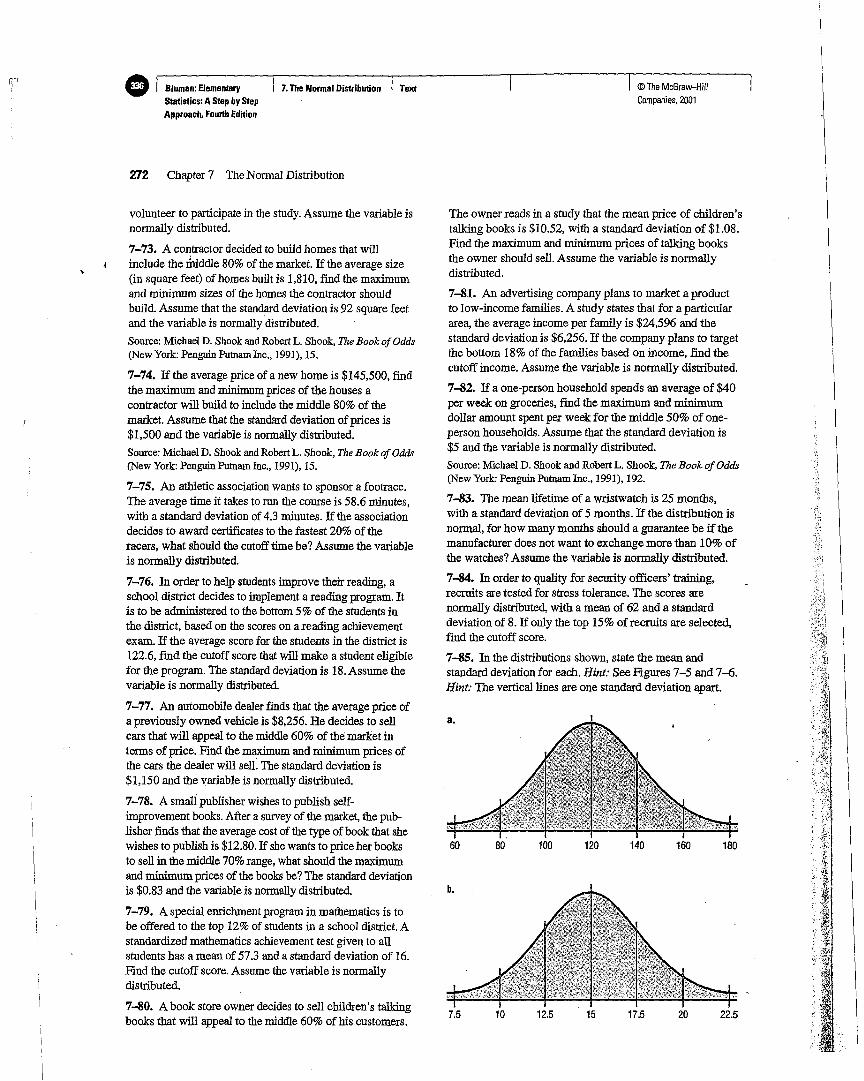
7-85. In the distributions shown, state the mean andstandard deviation for each. Hint: See Figures 7-5 and 7-6.Hint: The vertical lines are one standard deviation apart.
© The McGraw-HiliCompanies, 2001
7.TheNormal Distribution Texte Bluman: ElementaryStatistics:AStepbyStepApproach. Fourth Edition
rI

7-f,6. Suppose that the mathematics SAT scores for highschool seniors for a specific year have a mean of 456 anda standard deviation of 100 and are approximatelynormally distributed. If a subgroup of these high schoolseniors, those who are in the National Honor Society, isselected, would you expect the distribution of scores tohave the same mean and standard deviation? Explain youranswer.
7-f,7. Given a data set, how could you decide if thedistribution of the data was approximately normal?
7-f,8. If a distribution of raw scores were plotted and thenthe scores were transformed into zscores, would the shapeof the distribution change? Explain your answer.
7-f,9. In a normal distribution, find 0" when JL = 100 and2.68% of the area lies to the right of 105.
7-90. In a normal distribution, find JL when rr is 6 and3.75% of the area lies to the left of 85.
7-91. In a certain normal distribution, 1.25% of the arealies to the left of 42 and 1.25% of the area lies to the rightof 48. Find JL and 0".
7-92. An instructor gives a 100-point examination inwhich the grades are normally distributed. The mean is 60and the standard deviation is 10. If there are 5% Xs and 5%F's, 15% B's and 15% D's, and 60% C's, find the scoresthat divide the distribution into those categories.
© The McGraw-HiliCompanies, ZOOl
Section 7-4 Applications of the Normal Distribution 273
4035
The calculator will display .0268033499.
1 df ,',-, .-, 4.....nor~a c ~~,~. ("1.'
.0159944012nor-ma1cdf':: -1 E99,-1 q~ ...
• .I' --.1 ..•"::1--:''::: CI'-::1~"':!'4.~q• ".:.I..:.'_' .... ~.:. ...J •..J .'.'
Example TI7-1Find the area between z = 2.00 and z = 2.47, as in Example 7-6.
1. Press 2nd [DISTR] then 2 to get normalcdf (.2. Enter 2, 2.47) then press ENTER.
The calculator will display .0159944012.To find the area under the normal distribution curve less than (or greater than) any z value,
use -1E99 and 1E99 to specify infinity.
Example TI7-2Find the area to the left of z = -1.93, as in Example 7-5.
1. Press 2nd [DISTR] then 2 to get normalcdf (.2. Enter -lE99, -1.93) then press ENTER. Note: Use 2nd [EE] to paste E into the cursor
location (this indicates the following number-here, 99-is an exponent).
Tilll® l'T\tvlfi.m~n If)1l;sitdfu>wtl1\0llliTo find the area under the standard normal distribution curve between any two z values:
30
7.TheNormel Distribution Text
252015
. Blumen: ElementaryStBtistics: AStepbyStepApproech,Fourth Edition
TI·83Step by Step
-
o Bluman: ElementaryStatistics:AStep byStepApproach. Fourth Edition
7.TheNormal Distribution TeXl © The McGraw-HiliCompanies, 2001
274 Chapter 7 The Normal Distribution
.- '-'4.- C'S'-'791• b..::. f.:·oJ ... ..::. ..:J _
To find the area under a normal distribution curve between any two z values given a specificmean and standard deviation:
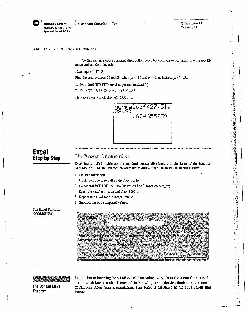
Example TI7-3Find the area between 27 and 31 when JL = 28 and (J" = 2, as in Example 7-15a.
1. Press 2nd [DISTR] then 2 to get normalcdf (.
2. Enter 27,31,28,2) then press ENTER.
The calculator will display .6246552391.
1. Select a blank cell.
2. Click the f x icon to call up the function list.
3. Select NORMSDIST from the Statistical function category.
4. Enter the smaller z value and click [OK].
5. Repeat steps 1-4 for the larger z value.
6. Subtract the two computed values.
Th~ r'f@rr"lffill&lH Di15lJ;!1"liblillti!@illlExcel has a built-in table for the standard normal distribution, in the form of the functionNORMSDIST. To find the area between two z values under the normal distribution curve:
In addition to knowing how individual data values vary about the mean for a population, statisticians are also interested in knowing about the distribution of the meansof samples taken from a population. This topic is discussed in the subsections thatfollow.
The Central LimitTheorem
ExcelStep by Step
The Excel FunctionNORMSDIST

© The McGraw-HiliCompanies, 2001
Section 7-5 The Central Limit Theorem 275
The following example illustrates these two properties. Suppose a professor gavean eight-point quiz to a small class of four students. The results of the quiz were 2, 6, 4,and 8. For the sake of discussion, assume that the four students constitute the population. The mean of the population is
11.=2+6+4+8=5f"" 4
When all possible samples of a specific size are selected with replacement from apopulation, the distribution of the sample means for a variable has two important properties, which are explained next.
Sampling error is the difference between the sample measure and the corresponding population measure dueto the fact that the sample isnot apertect representation of the populatlon,
If the samples are randomly selected with replacement, the sample means, for themost part, will be somewhat different from the population mean JL. These differencesare caused by sampling error.
Suppose a researcher selects 100 samples of a specific size from a large population andcomput~ ~ ~ean of ~e same variable for each of the 100 samples. These samplemeans, Xl> X2, X3, ..• , XlQO, constitute a sampling distribution of sample means.
Asampling distribution ofsample means isadistribution obtained by using the means computed fromrandom samples of aspecific size taken from apopulation.
The standard deviation of the population is
y(2 - 5)2 + (6 - 5)2 + (4 - 5)2 + (8 - 5)2c > = 2.236
4
The graph of the original distribution is shown in Figure 7-37. This is called a uniformdistribution.
7.The Normal Distribution TextSiuman: ElementaryStatistics: A Step byStepApproach. Fourth Edition
Distribution ofSampleMeansIliljeciille 6. Use the centrallimit theorem tosolveproblems involving samplemeans for large and smallsamples.
Figure 7-37
Distribution of QuizScores
2 4 6 8Score
Now, if all samples of size 2 are taken with replacement, and the mean ofeach sample is found, the distribution is as shown next.
o I 8luman: Elementary I 7.TheNormal Distribution I TextStatistics: A Step byStepApproach. Fourth Edition
276 Chapter 7 The Normal Distribution
© The McGraw-HiliCompanies. 2001
"
Sample Mean Sample Mean
2,2 2 6,2 42,4 3 6,4 52,6 4 6,6 62,8 5 6,8 74,2 3 8,2 54,4 4 8,4 64,6 5 8,6 74, 8 6 8,8 8
Figure 7-38Distribution ofSample Means
A frequency distribution of sample means is as follows.
X f2 13 24 35 46 37 28 1
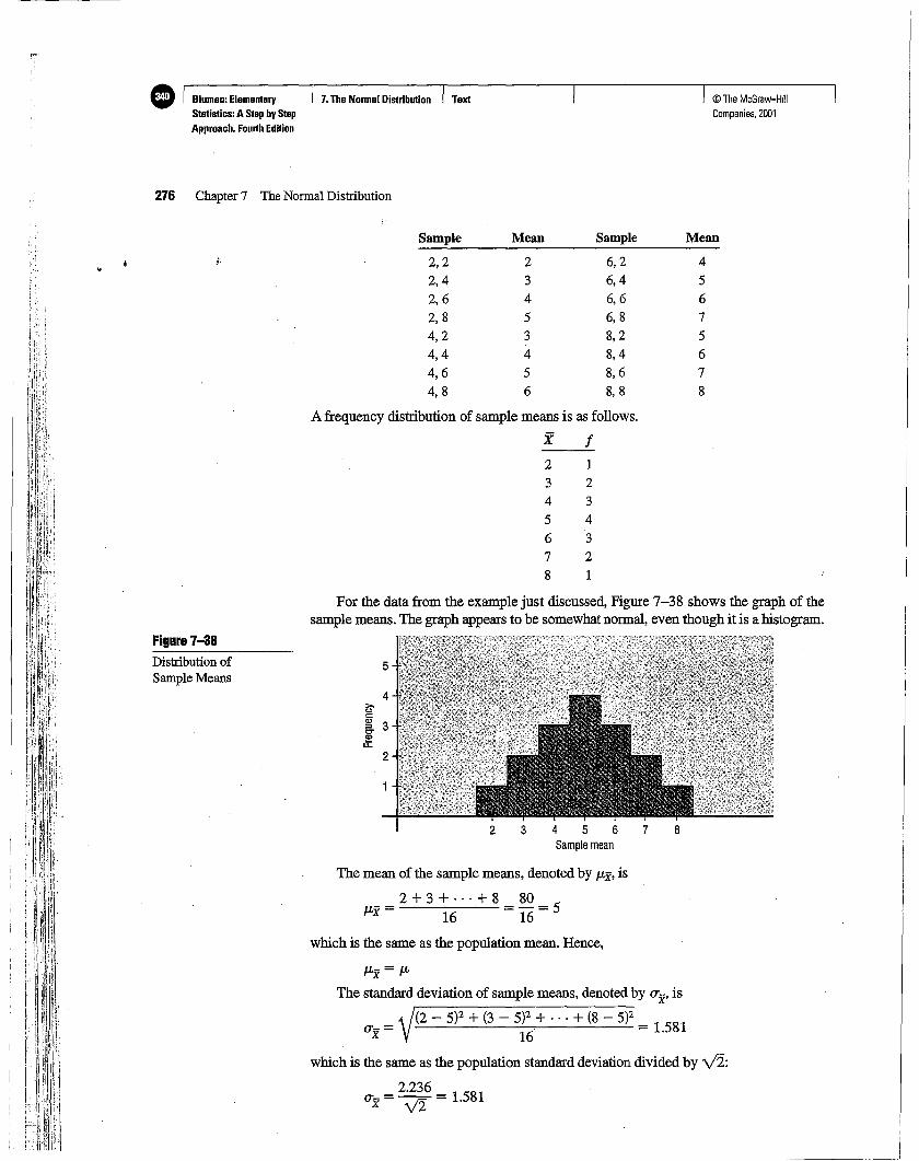
For the data from the example just discussed, Figure 7-38 shows the graph of thesample means. The graph appears to be somewhat normal, even though it is a histogram.
The mean of the sample means, denoted by /J.lg, is
2+3+ .. ·+880/Lx = 16 = 16 = 5
which is the same as the population mean. Hence,
/Lx = /L
The standard deviation of sample means, denoted by (Tx' is0\ /(2 - 5)2 + (3 - 5)2 + ... + (8 - 5)2
(Tx = V 16 = 1.581
which is the same as the population standard deviation divided by 0:
- 2.236 - 1 581(Tx - VI - .
Blumen: ElementaryStatistics: A Step byStepApproach. Fourth Edition
7.TheNormal Distribution Text © The McGraw-HiliCompanies. 2001
Section 7-5 The Central Limit Theorem 277
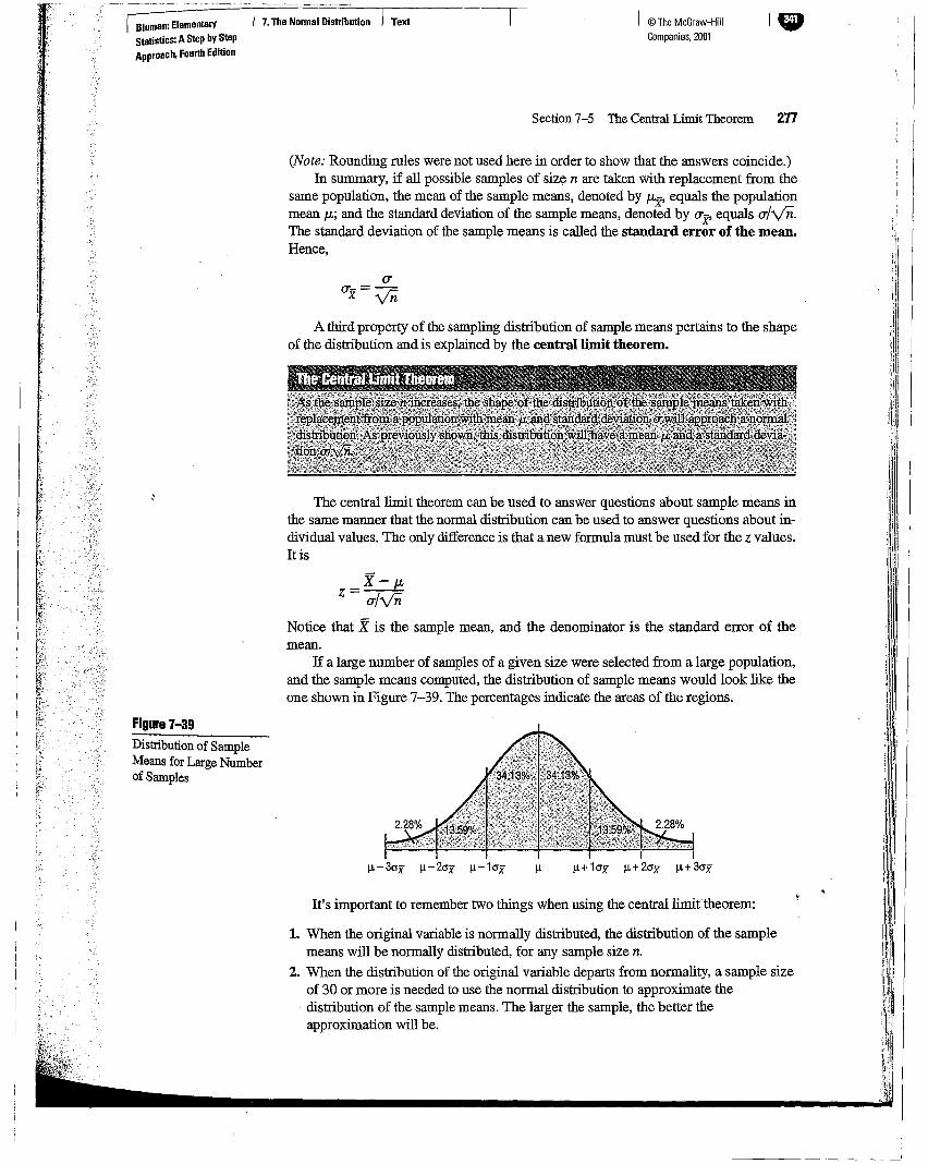
Il +1ax Il +2ax Il + 3ax
It's important to remember two things when using the central limittheorem:
1. When the original variable is normally distributed, the distribution of the samplemeans will be normally distributed, for any sample size n:
2. When the distribution of the original variable departs from normality, a sample sizeof 30 or more is needed to use the normal distribution to approximate thedistribution of the sample means. The larger the sample, the better theapproximation will be.
The central limit theorem can be used to answer questions about sample means inthe same manner that the normal distribution can be used to answer questions about individual values. The only difference is that a new formula must be used for the zvalues.It is
CTCTX = Vii
A third property of the sampling distribution of sample means pertains to the shapeof the distribution and is explained by the central limit theorem.
(Note: Rounding rules were not used here in order to show that the answers coincide.)In summary, if all possible samples of size n are taken with replacement from the
same population, the mean of the sample means, denoted by JLx' equals the populationmean JL; and the standard deviation of the sample means, denoted by CTi' equals a/Vn.The standard deviation of the sample means is called the standard error of the mean.Hence,
X-JLz=--CT/ViiNotice that X is the sample mean, and the denominator is the standard error of themean.
If a large number of samples of a given size were selected from a large population,and the sample means computed, the distribution of sample means would look like theone shown in Figure 7-39. The percentages indicate the areas of the regions.
Distribution of SampleMeans for Large Numberof Samples
Figure 7-39
Blumsn:ElementaryStatistics:AStepby StepApproach,FnurthEdition
7.TheNormal Distribution Text © The McGraw-HiliCompanies. 2001
278 Chapter 7 The Nonna! Distribution
26.325
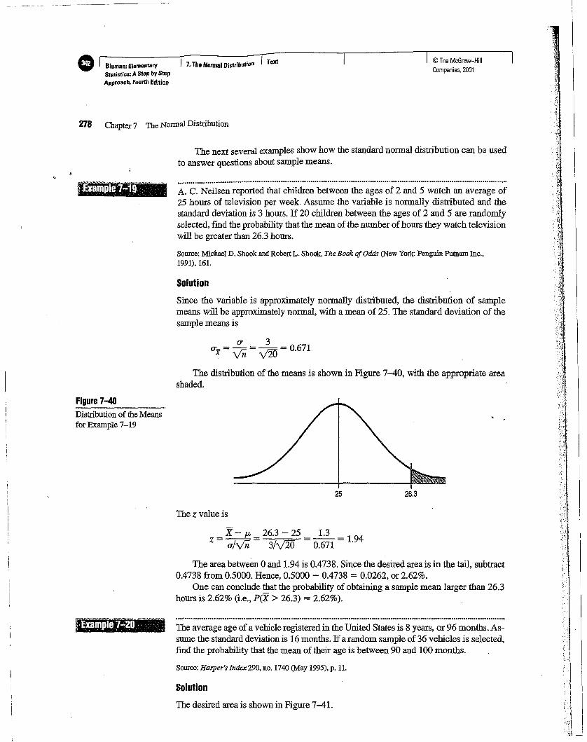
x - p: 26.3 - 25 1.3z = U'/Vii = 3/VW = 0.671 = 1.94
The next several examples show how the standard normal distribution can be usedto answer questions about sample means .
A. C. Neilsen reported that children between the ages of 2 and 5 watch an average of25 hours of television per week. Assume the variable is normally distributed and thestandard deviation is 3 hours. If20 children between the ages of 2 and 5 are randomlyselected, [rod the probability that the mean of the number ofhours they watch televisionwill be greater than 26.3 hours.
Since the variable is approximately normally distributed, the distribution of samplemeans will be approximately normal, with a mean of 25. The standard deviation of thesample means is
U' 3U'jf = Vii = VW = 0.671
Solution
...............................................................................................................................................................................
Source: Michael D. Shook and Robert L. Shook, The Book ofOdds (New York: Penguin Putnam Inc.,1991),161.
The z value is
The distribution of the means is shown in Figure 7-40, with the appropriate areashaded.
The area between 0 and 1.94 is 0.4738. Since the desired area is in the tail, subtract0.4738 from 0.5000. Hence, 0.5000 - 0.4738 = 0.0262, or 2.62%.
One can conclude that the probability of obtaining a sample mean larger than 26.3hours is 2.62% (i.e., p(Jt. > 26.3) = 2.62%).
Source: Harper's Index 290, no. 1740 (May 1995), p. 11.
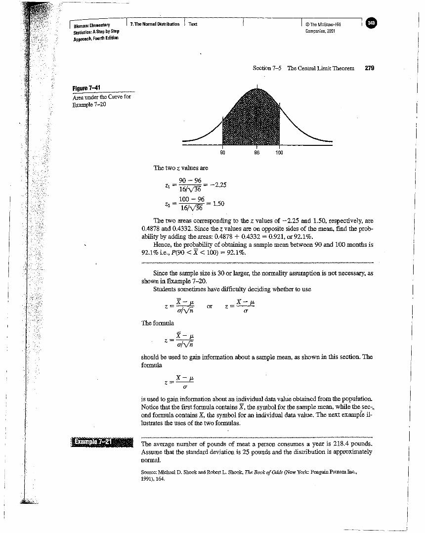
The desired area is shown in Figure 7-41.
Solution
The average age of a vehicle registered in the United States is 8 years, or 96 months. Assume the standard deviation is 16 months. Ifa random sample of 36 vehicles is selected,:find the probability that the mean of their age is between 90 and 100 months.
Figure 7-40Distribution of the Meansfor Example 7-19
should be used to gain information about a sample mean, as shown in this section. Theformula
X-p,z=-(F
100
© The McGraw-HiliCompanies. 2001
96
Section 7-5 The Central Limit Theorem 279
X-p,z=-(F
orf-p,
z=--a/Vii
f- p,z=--a/Vii
The formula
Since the sample size is 30 or larger, the normality assumption is not necessary, asshown in Example 7-20.
Students sometimes have difficulty deciding whether to use
The two areas corresponding to the Z values of -2.25 and 1.50, respectively, are0.4878 and 0.4332. Since the z values are on opposite sides of the mean, find the probability by adding the areas: 0.4878 + 0.4332 = 0.921, or 92.1%.
Hence, the probability of obtaining a sample mean between 90 and 100 months is92.1% i.e., P(90 < f < 100) = 92.1%.
7.TheNormal Distribution Text
90
Bluman: ElementaryStatistics: AStep byStepApproach, Fourth Edition
The two Z values are
90 - 96Zl = 16/v'36 = -2.25
100 - 96Zz = 16/v'36 = 1.50
Areaunder the Curve forExample 7-20
Figure 7-41
-is used to gain information about an individual data value obtained from the population.Notice that the first formula contains X, the symbol for the sample mean, while the sec-,ond formula contains X, the symbol for an individual data value. The next example illustrates the uses of the two formulas.
The average number of pounds of meat a person consumes a year is 218.4 pounds.Assume that the standard deviation is 25 pounds and the distribution is approximatelynormal.
Source: Michael D. Shook and Robert L. Shook, The Book ofOdds (New York: Penguin Putnam Inc.,1991),164.

280 Chapter 7 The Normal Distribution
Solution
© The McGraw-HiliCompanies. 2001
7.TheNormal Distribution Text
218;4 224Distribution ofmeans forallsamples ofsize 40taken from the population
The z value is
The area between 0 and 0.22 is 0.0871; this area must be added to 0.5000 to get thetotal area to the left of z = 0.22.
z = X : p., = 224 ~5218.4 = 0.22
218;4 224Distribution ofindividual data values forthe population
0.0871 + 0.5000 = 0.5871
a. Find the probability that a person selected at random consumes less than 224pounds per year.
b. If a sample of 40 individuals is selected, find the probability that the mean of thesample will be less than 224 pounds per year.
a. Since the question asks about an individual person, the formula z = (X - p.,)1ais used.
The distribution is shown in Figure 7-42.
Hence, the probability of selecting an individual who consumes less than 224pounds of meat per year is 0.5871, or 58.71 % (i.e., P(X < 224) = 0.5871).
b. Since the question concerns the mean of a sample with a size of 40, the formulaz = (X - p.,)/(u/vn) is used.
The area is shown in Figure 7-43.
Figure 7-42Area under.the Curve forPart a of Example 7-21
Area under the Curve forPart b of Example 7-21
Figure 7-43
e Bluman: ElementaryStatistics:AStepbyStepApproach. Fourth Edition
Bluman: ElementaryStatistics: AStepbyStepApproach, Fourth Edition
7.TheNormal Distribution Text
The z value is
©The McGraw-HiliCompanies, 2001
Section 7-5 The CentralLimit Theorem 281
X-JL
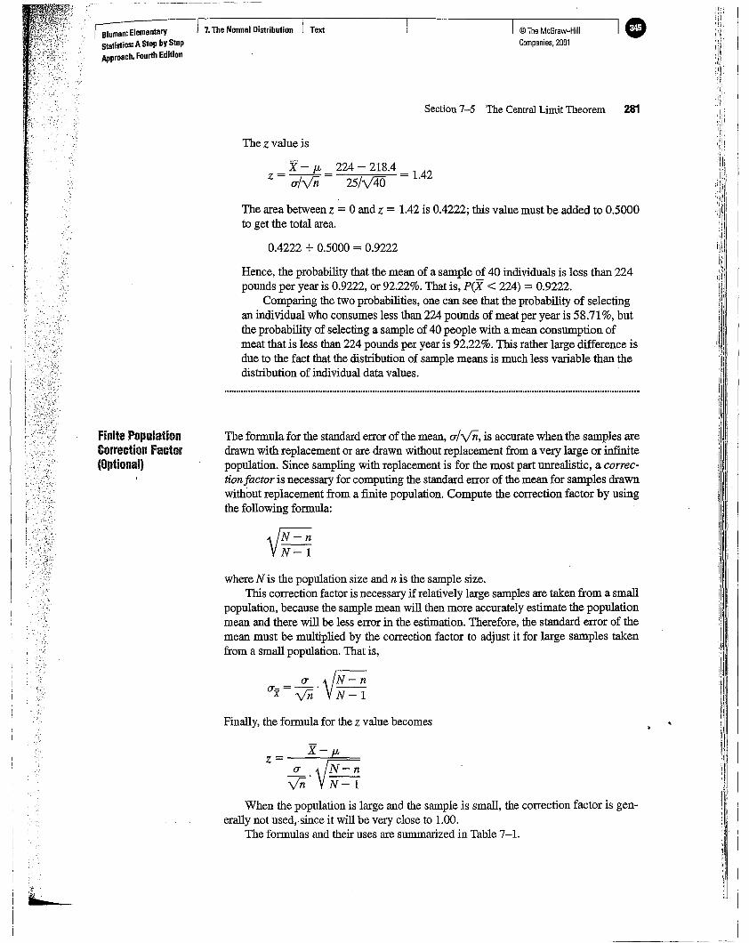
z= a ~-nyn' N- 1
Finally, the formula for the z value becomes
1~VN=1
The area between z = 0 and z = 1.42 is 0.4222; this value must be added to 0.5000to get the total area.
= X- JL = 224 - 218.4 = 1 42z cr/yn 25/V45 .
Hence, the probability that the mean of a sample of 40 individuals is less than 224pounds per year is 0.9222, or 92.22%. That is, P(X < 224) = 0.9222.
Comparing the two probabilities, one can see that the probability of selectingan individual who consumes less than 224 pounds of meat per year is 58.71%, butthe probability of selecting a sample of 40 people with a mean consumption ofmeat that is less than 224 pounds per year is 92.22%. This rather large difference isdue to the fact that the distribution of sample means is much less variable than thedistribution of individual data values.
0.4222 + 0.5000 = 0.9222
The formula for the standard error of the mean, cr/yn, is accurate when the samples aredrawn with replacement or are drawn without replacement from a very large or infinitepopulation. Since sampling with replacement is for the most part unrealistic, a correctionfactor is necessary for computing the standard error of the mean for samples drawnwithout replacement from a finite population. Compute the correction factor by usingthe following formula:
where N is the population size and n is the sample size.This correction factor is necessary if relatively large samples are taken from a small
population, because the sample mean will then more accurately estimate the populationmean and there will be less error in the estimation. Therefore, the standard error of themean must be multiplied by the correction factor to adjust it for large samples takenfrom a small population. That is,
When the population is large and the sample is small, the correction factor is generally not used,since it will be very close to 1.00.
The formulas and their uses are summarized in Table 7-1.
finite PopulationCorrection factor(Optional)

41) , 8luman: Elementary I 7.TheNormal Distribution I TextStatistics:AStep bV StepApproach. Fourth Edition
282 Chapter 7 The Normal Distribution
© The McGraw-HiliCompanies. 2001
-
7-93. If samples of a specific size are selected from apopulation and the means are computed, what is thisdistribution of means called?
7-94. Why do most of the sample means differ somewhatfrom the population mean? What is this difference called?
7-95. What is the mean of the sample means?
7-96. What is the standard deviation of the sample meanscalled? What is the formula for this standard deviation?
7-97. What does the central limit theorem say about theshape of the distribution of sample means?
7-98. What formula is used to gain information about anindividual data value when the variable is normallydistributed?
7-99. What formula is used to gain information about asample mean when the variable is normally distributed orwhen the sample size is 30 or more?
For Exercises 7-100 through 7-117, assume that thesample is taken from a large population and thecorrection factor can be ignored.
7-100. A survey found thatAmericans generate an averageof 17.2 pounds of glass garbage each year. Assume thestandard deviation of the distribution is 2.5 pounds. Findthe probability that the mean of a sample of 55 families willbe between 17 and 18 pounds.
Source:MichaelD. Shookand Robert L. Shook,TheBook ofOdds(New York: Penguin PutnamInc., 1991),14.
7-101. The mean serum cholesterol of a large populationof overweight adults is 220 mg/dl and the standarddeviation is 16.3 mg/dl, If a sample of 30 adults is selected,fmd the probability that the mean will be between 220 and222mg/dl.
7-102. For a certain large group of individuals, the meanhemoglobin level in the blood is 21.0 grams per milliliter(g/ml). The standard deviation is 2 g/mI. If a sample of 25
individuals is selected, find the probability that the meanwill be greater than 21.3 g/ml. Assume the variable isnormally distributed.
7-103. The mean weight of 18-year-old females is 126pounds, and the standard deviation is 15.7. If a sample of25 females is selected, find the probability that the mean-ofthe sample will be greater than 128.3 pounds. Assume thevariable is normally distributed.
7-104. The mean grade point average of the engineeringmajors at a large university is 3.23, with a standarddeviation of 0.72. In a class of 48 students, find theprobability that the mean grade point average of thestudents is less than 3.15.
7-105. The average price of a pound of sliced bacon is$2.02. Assume the standard deviation is $0.08. If a randomsample of 40 one-pound packages is selected, find theprobability that the mean of the sample will be less than$2.00.
Source: Statistical Abstract ofthe United States 1994.(Washington, DC: U. S. Bureau of the Census).
7-106. The average hourly wage of fast-food workersemployed by a nationwide chain is $5.55. The standarddeviation is $1.15. If a sample of 50 workers is selected,find the probability that the mean of the sample will bebetween $5.25 and $5.90.
7-107. The mean score on a dexterity test for12-year-olds is 30. The standard deviation is 5. If apsychologist administers the test to a class of 22students, find the probability that the mean of the samplewill be between 27 and 31. Assume the variable isnormally distributed.
7-108. A recent study of the life span of portable radiosfound the average to be 3.1 years, with a standarddeviation of 0.9 year. If the number of radios owned bythe students in one dormitory is 47, find the probability
that the mean lifetime of these radios will be less than
2.7 years.
7-109. The average age oflawyers is 43.6 years, with astandard deviation of 5.1 years. If a law firm employs 50lawyers, find the probability that the average age of thegroup is greater than 44.2 years old.
7-110. The average annual precipitation for Des Moines is30.83 inches, with a standard deviation of 5 inches. If arandom sample of 10 years is selected, find the probabilitythat the mean will be between 32 and 33 inches. Assumethe variable is normally distributed.
7-111. Procter & Gamble reported that an American familyof 4 washes an average of one ton (2000 pounds) of clotheseach year. If the standard deviation of the distribution is187.5 pounds, find the probability that the mean of arandomly selected sample of 50 families of four will bebetween 1980 and 1990 pounds.
Source: Lewis H.Lapham, MichaelPollan, andEric Etheridge,The Harper's Index Book (NewYork: Henry Holt & Co., 1987).
7-112. The average annual salary in Pennsylvania was$24,393 in 1992. Assume that salaries were normallydistributed for a certain group of wage earners, and thestandard deviation of this group was $4,362.a. Find the probability that a randomly selected individual
earned less than $26,000.b. Find the probability that for a randomly selected sample
of 25 individuals, the mean salary was less than $26,000.c. Why is the probability for Part b higher than the
probability for Part a?
Associated Press,December23, 1992.
7-113. The average time it takes a group of adults tocomplete a certain achievement test is 46.2 minutes. Thestandard deviation is 8 minutes. Assume the variable isnormally distributed.a. Find the probability that a randomly selected adult will
complete the test in less than 43 minutes.b. Find the probability that if 50 randomly selected adults
take the test, the mean time it takes the group to completethe test will be less than 43 minutes.c. Does it seem reasonable that an adult would finish the
test in less than 43 minutes? Explain.d. Does it seem reasonable that the mean of the 50 adults
could be less than 43 minutes?
7-114. Assume that the mean systolic blood pressure ofnormal adults is 120 millimeters of mercury (mm Hg) andthe standard deviation is 5.6. Assume the variable isnormally distributed.a. If an individual is selected, find the probability
that the individual's pressure will be between 120 and121.8 lIllIl Hg.
8luman: ElementaryStatistics: AStep byStepApproach. Fourth Edition
7.TheNormal Distribution Text ©The McGraw-HiliCompanies, 2001
Section 7-5 The Central Limit Theorem 283
b. If a sample of 30 adults is randomly selected, find theprobability that the sample mean will be between 120 and121.8 lIllIl Hg.c. Why is the answer to Part a so much smaller than the
answer to Part b?
7-115. The average cholesterol content of a certainbrand of eggs is 215 milligrams and the standarddeviation is 15 milligrams. Assume the variable isnormally distributed.a. If a single egg is selected, find the probability that the
cholesterol content will be more than 220 milligrams.b. If a sample of 25 eggs is selected, find the probability
that the mean of the sample will be larger than 220milligrams.
Source:LivingFit (EnglewoodCliffs,NJ: Best Foods, CPCInternational, Inc., 1991).
7-116. At a large publishing company, the mean age ofproofreaders is 36.2 years, and the standard deviation is 3.7years. Assume the variable is normally distributed.a. If a proofreader from the company is randomly
selected, find the probability that his or her age will bebetween 36 and 37.5 years.b. If a random sample of 15 proofreaders is selected, find
the probability that the mean age of the proofreaders in thesample will be between 36 and 37.5 years.
7-117. The average labor cost for car repairs for alarge chain of car repair shops is $48.25. The standarddeviation is $4.20. Assume the variable is normallydistributed.a. If a store is selected at random, find the probability thatthe labor cost will range between $46 and $48.b. If 20 stores are selected at random, find the
probability that the mean of the sample will be between$46 and $48.c. Which answer is larger? Explain why.
For Exercises 7-118 and 7-119, check to see whether thecorrection factor should be used. H so, be sure toinclude it in the calculations.
*7-118. In a study of the life expectancy of 500 people in acertain geographic region, the mean age at death was 72.0years and the standard deviation was 5.3 years. If a sampleof 50 people from this region is selected, find theprobability that the mean life expectancy will be less than70 years.
*7-119. A study of 800 homeowners in a certain areashowed that the average value of the homes was $82,000
.and the standard deviation was $5,000. If 50 homes are forsale, find the probability that the mean of the values ofthese homes is greater than $83,500.
o I Bluman: Elementary I 7.TheNormal Distribution I TextStatistics:AStep byStepApproach. Fourth Edition
284 Chapter 7 The Normal Distribution
*7-120. The average breaking strength of a certainbrand of steel cable is 2000 pounds, with a standarddeviation of 100 pounds. A sample of 20 cables isselected and tested. Find the sample mean that will cutoff the upper 95% of all of the samples of size 20 takenfrom the population. Assume the variable is normallydistributed.
© The McGraw-HiliCompanies, 2001
*7-121. The standard deviation of a variable is 15. If asample of 100 individuals is selected, compute the standarderror of the mean. What size sample is necessary to doublethe standard error of the mean?
*7-122. In Exercise 7-121, what size sample is needed tocut the standard error of the mean in half?
The NormalApproximation totheBinomial Distribution
f]lij<lctive 1. Use the normalapproximation tocomputeprobabilities forabinomialvariable.
The normal distribution is often used to solve problems that involve the binomial distribution since when n is large (say, 100), the calculations are too difficult to do by handusing the binomial distribution. Recall from Chapter 6 that a binomial distribution hasthe following characteristics:
1. There must be a fixed number of trials.
2. The outcome of each trial must be independent.
3. Each experiment can have only two outcomes or be reduced to two outcomes.
4. The probability of a success must remain the same for each trial.
Also, recall that a binomial distribution is determined by n (the number of trials)andp (the probability of a success). Whenp is approximately 0.5, and as nincreases, theshape of the binomial distribution becomes similar to the normal distribution. The largern and the closer p is to 0.5, the more similar the shape of the binomial distribution is tothe normal distribution.
But when p is close to 0 or 1 and n is relatively small, the normal approximation isinaccurate. As a rule of thumb, statisticians generally agree that the normal approximation should be used only when n . p and n . q are both greater than or equal to 5. (Note:q = 1 - p.) For example, ifpis 0.3 and n is 10, then np = (10)(0.3) = 3, and the normal distribution should not be used as an approximation. On the other hand, ifp = 0.5and n = 10, then np = (10)(0.5) = 5 and nq = (10)(0.5) = 5, and the normal distribution can be used as an approximation. See Figure 7-44.
In addition to the previous condition of np ;::: 5 and nq ;::: 5, a correction for continuity may be used in the normal approximation.
Acorrection for continuity isacorrection employed when acontinuous distribution is used toapproximate adiscrete distribution.
The continuity correction means that for any specific value of X, say 8, theboundaries of X in the binomial distribution (in this case, 7.5 to 8.5) must be used. (SeeChapter 1, Section 1-3.) Hence, when one employs the normal distribution to approximate the binomial, the boundaries of any specific value X must be used as they areshown in the binomial distribution. For example, for P(X = 8), the correction isP(7.5 < X < 8.5). For P(X:5 7), the correction is P(X < 7.5). For P(X;::: 3), the correction is P(X > 2.5).
Students sometimes have difficulty deciding whether to add 0.5 or subtract 0.5from the data value for the correction factor. Table 7-2 summarizes the differentsituations.

X
9
x P(X)
o 0.0281 0.1212 0.2333 0.2674 0.2005 0.1036 0.0377 0.0098 0.0019 0.000
10 0.000
© The McGraw-HiliCompanies, 2001
B76543
Binomial Probabilities forn=10, p=0.3In·p= 10(0.3) =3;n»q=10(0.7) =7]
2o
Section 7-6 The Normal Approximation to the Binomial Distribution 285
P(X)
0.2
0.3
x0 2 3 4 5 6 7 B 9 10
P(X) Binomial Probabilities forn=10, P=0.5In·p= 10(0.5),= 5;n»q= 10(0.5) =5]
0.3
X P(X)
0 0.0011 0.010
0.2 2 0.0443 0.1174 0.2055 0.2466 0.2057 0.117B 0.044
0.1 9 0.01010 0.001
0.1
7.TheNormal Distribution TextBluman: ElementaryStatistics: AStepbyStepApproach, Fourth Edition
Comparison of theBinomial Distribution andthe Normal Distribution
Figure 7-44
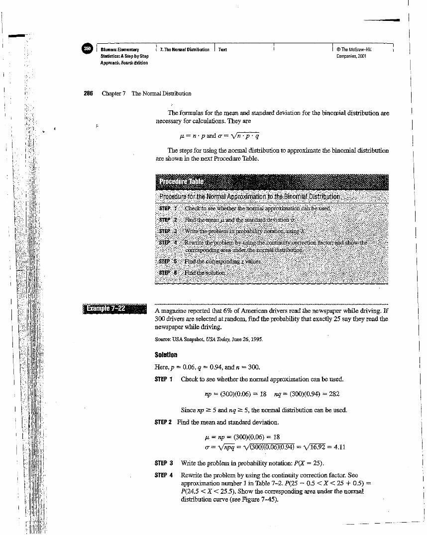
,.
e I Bluman: Elementary I 7.The Normal Distribution I TextStatistics:AStepbyStepApproach. Fourth Edition
•
I © The McGrew-HiliCompenies, 2001
The formulas for the mean and standard deviation for the binomial distribution arenecessary for calculations. They are
J.L = n . p and a = \/n . p . q
J.L = np = (300)(0.06) = 18
tr = ynpq = \/(300)(0.06)(0.94) = \116.92 = 4.11
np = (300)(0.06) = 18 nq = (300)(0.94) = 282
The steps for using the normal distribution to approximate the binomial distributionare shown in the next Procedure Table.
A magazine reported that 6% of American drivers read the newspaper while driving. If300 drivers are selected at random, find the probability that exactly 25 say they read thenewspaper while driving.
STEP 3 Write the problem in probability notation: P(X = 25).
STEP 4 Rewrite the problem by using the continuity correction factor. Seeapproximation number 1 in Table 7-2. P(25 - 0.5 < X < 25 + 0.5) =P(24.5 < X < 25.5). Show the corresponding area under the normaldistribution curve (see Figure 7-45).
Since np :::: 5 and nq :::: 5, the normal distribution can be used.
STEP 2 Find the mean and standard deviation.
Source: USASnapshot, USAToday, June26, 1995.
Solution
Here, p = 0.06, q = 0.94, and n = 300.
STEP 1 Check to see whether the normal approximation can be used.
Chapter 7 The Normal Distribution286
! ample"7-22 ~
_......
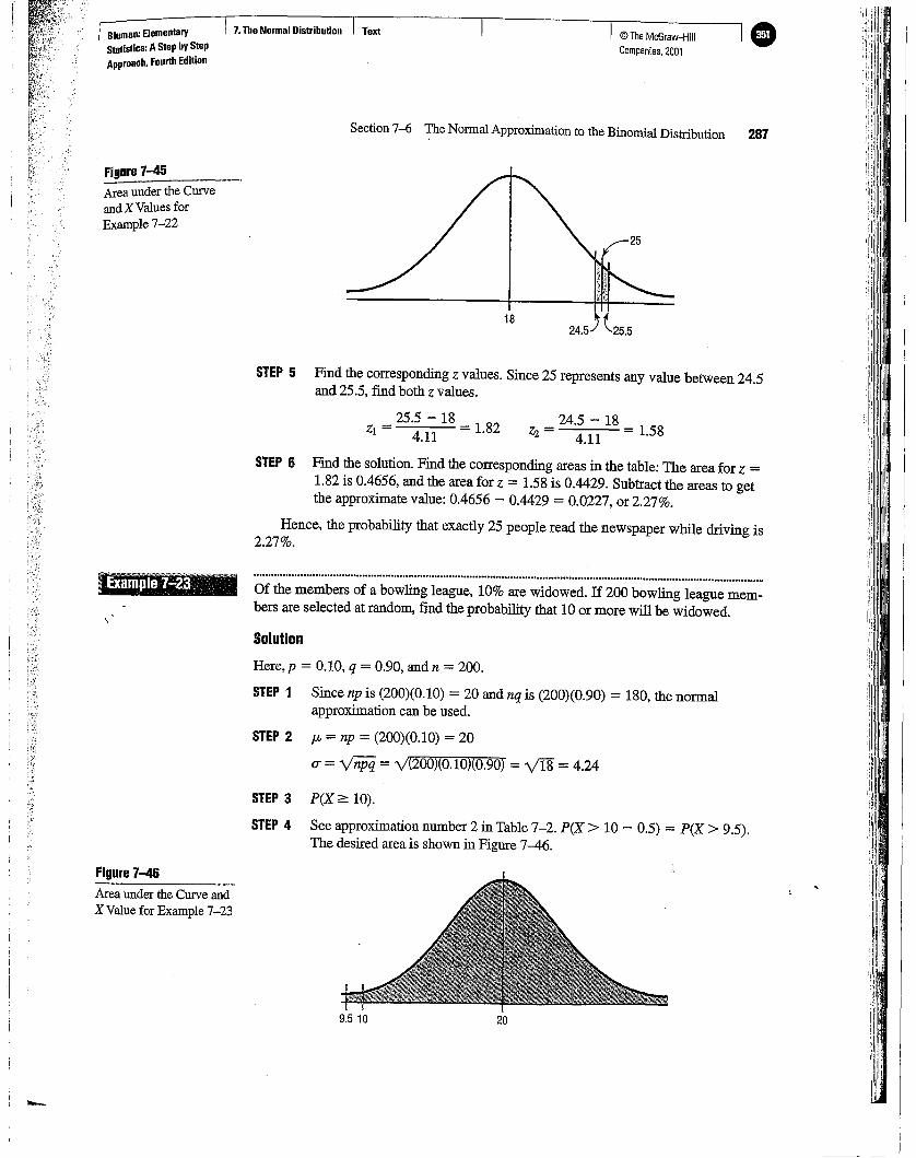
Section 7-6 The Normal Approximation to the Binomial Distribution 287
© The McGraw-HiliCompanies. 2001
= 24.5 - 18 = 1 58Zz 4.11 .
20
= 25.5 - 18 = 1 82Zl 4.11 .
9.510
Of the members of a bowling league, 10% are widowed. If 200 bowling league members are selected at random, find the probability that 10 or more will be widowed.
STEP 5 Find the corresponding z values. Since 25 represents any value between 24.5and 25.5, find both z values.
18 24.5 (25.5
STEP 6 Find the solution. Find the corresponding areas in the table: The area for z =1.82 is 0.4656, and the area for z = 1.58 is 0.4429. Subtract the areas to getthe approximate value: 0.4656 - 0.4429 = 0.0227, or 2.27%.
Hence, the probability that exactly 25 people read the newspaper while driving is2.27%.
.............................................................................................................................................................................
Solution
Here,p = 0.10, q = 0.90, andn = 200.
STEP 1 Since np is (200)(0.10) = 20 and nq is (200)(0.90) = 180, the normalapproximation can be used.
STEP 2 JL = np = (200)(0.10) = 20
(J' = vnpq = y'(200)(0.1O)(0.90) = y18 = 4.24
STEP 3 P(X ~ 10).
STEP 4 See approximation number 2 in Table 7-2. P(X> 10 - 0.5) = P(X> 9.5).The desired area is shown in Figure 7-46.
7.TheNormal Distribution TextBluman: ElementaryStatistics: AStepbyStepApproach, Fourth Edition
Figure 7-45Area under the Curveand X Values forExample 7-22
. ample7-2
Figure 7-46
Area under the Curve andX Value for Example 7-23
-

CD Bluman:Elemelll8ry 7.The Normal Distribution Text
Statistics: A Step by Step
Approach,FourthEdition
288 Chapter 7 The Normal Distribution
© The McGraw-HiliCompanies, 2001
Figure 7-47Area under the Curve forExample 7-24
STEP 5 Since the problem is to find the probability of 10 or more positive responses,the normal distribution graph is as shown in Figure 7-46. Hence, the areabetween 9.5 and 20 must be added to 0.5000 to get the correctapproximation.
The z value is
= 9.5 - 20 = -248z 4.24 .
STEP 6 The area between 20 and 9.5 is 0.4934. Thus, the probability of getting 10 ormore responses is 0.5000 + 0.4934 = 0.9934, or 99.34%.
It can be concluded, then, that the probability of 10 or more widowed people in arandom sample of 200 bowling league members is 99.34%.
If a baseball player's batting average is 0.320 (32%), find the probability that the playerwill get at most 26 hits in 100 times at bat.
Solution
Here, p = 0.32, q = 0.68, and n = 100.
STEP 1 Since np = (100)(0.320) = 32 and nq = (100)(0.680) = 68, the normaldistribution can be used to approximate the binomial distribution.
STEP 2 p: = np = (100)(0.320) = 32(T = yTijiq = Y(I00)(0.32)(0.68) = Y21.76 = 4.66
STEP 3 P(X:5 26).
STEP 4 See approximation number 4 in Table 7-2. P(X < 26 + 0.5) = P(X < 26.5).The desired area is shown in Figure 7-47.
26 26.5 32.0
STEP 5 The z value is
= 26.5 - 32 = -1 18z 4.66 .
STEP 6 The area between the mean and 26.5 is 0.3810. Since the area in the left tailis desired, 0.3810 must be subtracted from 0.5000. So the probability is0.5000....; 0.3810 = 0.1190, or 11.9%.
The closeness of the normal approximation is shown in the next example.
,\
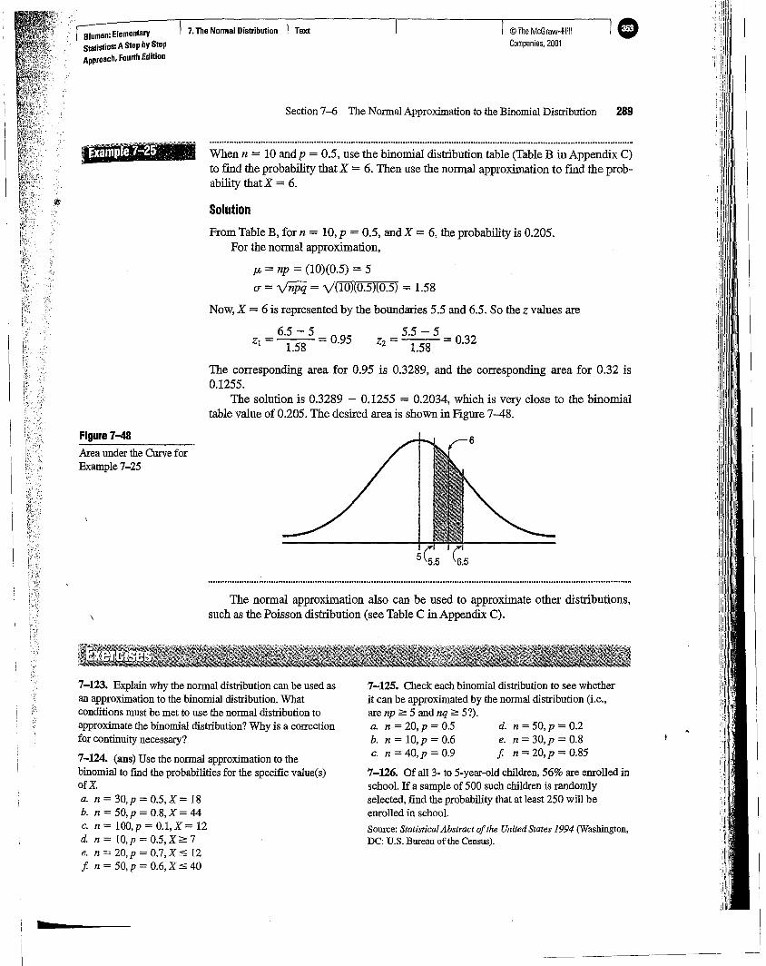
© The McGrew-HiliCompanies, 2001
5.5 - 5Zz = 1.58 =0.32
7-125. Check each binomial distributionto see whetherit can be approximatedby the normaldistribution (i.e.,are np 2=: 5 and nq 2=: 5?).a. n = 20,p = 0.5 d. n = 50,p = 0.2b. n = 1O,p = 0.6 e. n = 30,p = 0.8-c. n = 40,p = 0.9 f. n = 20,p = 0.85
7-126. Of al13- to 5-year-oldchildren, 56% are enrolled inschool. If a sample of 500 such childrenis randomlyselected, find the probabilitythat at least 250 will beenrolled in school.Source: Statistical Abstract ofthe United States 1994 (Washington,DC: U.S. Bureau of the Census).
6.5 - 5Zl = 1.58 = 0.95
p, = np = (10)(0.5) = 5
(T = ynpq = \1(10)(0.5)(0.5) = 1.58
Now, X = 6 is represented by the boundaries 5.5 and 6.5. So the zvalues are
Section 7-6 The Normal Approximationto the BinomialDistribution 289
When n = 10 and p = 0.5, use the binomial distribution table (Table B in Appendix C)to [rod the probability that X = 6. Then use the normal approximation to [rod the probability that X = 6.
Solution
From Table B, for n = 10, p =0.5, and X = 6, the probability is 0.205.For the normal approximation,
The corresponding area for 0.95 is 0.3289, and the corresponding area for 0.32 is0.1255.
The solution is 0.3289 - 0.1255 = 0.2034, which is very close to the binomialtable value of 0.205. The desired area is shown in Figure 7-48.
The normal approximation also can be used to approximate other distributions,such as the Poisson distribution (see Table C in Appendix C).
7.TheNormal Distribution Text8luman: ElementaryStatistics: AStepbyStepApproach, Fourth Edition
I .
Areaunder the CurveforExample7-25
Figure 7-48
7-123. Explainwhy the normal distributioncan be used asanapproximation to the binomial distribution. Whatconditionsmustbe met to use the normal distributiontoapproximatethe binomialdistribution?Why is a correctionfor continuitynecessary?
7-124. (ans) Use the normal approximation to thebinomial to find the probabilitiesfor the specific value(s)ofX.a. n = 30,p = O.5,X= 18b. n = 50,p = 0.8,X = 44c. n=l00,p=O.I,X= 12d. n = 1O,p = 0.5,X 2=: 7e. n=20,p=0.7,XSl2f. n = 50,p = 0.6, X s 40
>
e Bluman: ElementaryStatistics:AStepbyStepApproach. Fourth Edition
7.TheNormal Distribution Text © The McGraw-HiliCompanies, 2001
The normal distribution can be used to describe a variety of variables, such as heights,weights, and temperatures. The normal distribution is bell-shaped, unimodal, symmetric, and continuous; its mean, median, and mode are equal. Since each variable has itsown distribution with mean p, and standard deviation CT, mathematicians use the standard normal distribution, which has a mean of 0 and a standard deviation of 1. Other approximately normally distributed variables can be transformed into the standard normaldistribution with the formula z = (X - p,)/CT.
The normal distribution can also be used to describe a sampling distribution of sample means. These samples must be of the same size and randomly selected with replacement from the population. The means of the samples will differ somewhat from thepopulation mean, since samples are generally not perfect representations of the population from which they came. The mean of the sample means will be equal to the population mean, and the standard deviation of the sample means will be equal to thepopulation standard deviation divided by the square root of the sample size. The centrallimit theorem states that as the size of the samples increases, the distribution of samplemeans will be approximately normal.
The normal distribution can be used to approximate other distributions, such as thebinomial distribution. For the normal distribution to be used as an approximation, theconditions np ;::: 5 and nq ;::: 5 must be met. Also, a correction for continuity may beused for more accurate results.
290 Chapter 7 The Normal Distribution
7-127. Twoout of five adult smokers acquiredthe habit byage 14.If 400 smokers are randomly selected,find theprobabilitythat 170 or more acquired the habit by age 14.
Source: Harper's Index 289, no. 1735 (December 1994).
7-128. A theater ownerhas found that 5% of his patronsdo not showup for the performancethat they purchasedtickets for.If the theatrehas 100 seats, find the probabilitythat six or more patrons will not showup for the sold-outperformance.
7-129. In a survey, 15%of Americans said they believethat they will eventuallyget cancer.In a random sampleof80Americansused in the survey,find these probabilities.a. At least six people in the samplebelieve they will get
cancer.b. Fewer than five people in the samplebelieve they will
get cancer.Source: Harper's Index (December 1994), p. 13.
7-130. If the probability that a newborn child will befemale is 50%, find the probabilitythat in 100births,55 ormore will be females.
7-131. Prevention magazinereports that 18% of driversuse a car phone while driving.Find the probabilitythat in arandom sample of 100 drivers,exactly 18 will use a carphone while driving.
Source: USA Snapshot, USA Today, June 26, 1995.
7-132. A contractor statesthat 90% of all homes soldhaveburglar alarm systems. If a contractor sells 250 homes,find
Summary
the probability that fewer than 5 of them will not haveburglar alarmsystems.
7-133. In 1993,only 3% of elementary andsecondaryschoolsin the United States did not havemicrocomputers. If a random sample of 180 elementaryand secondaryschools is selected, find the probabilitythat in 19936 or fewer schools did not havemicrocomputers.
Source: Statistical Abstract of the United States 1994.(Washington, DC: U. S. Bureau of the Census).
7-134. Last year, 17% of American workers carpooledto work. If a random sample of 30 workers is selected,find the probabilitythat exactly 5 people will carpool towork.Source: USA Snapshot, USA Today, July 6, 1995.
7-135. Apolitical candidate estimates that 30% of thevoters in his party favor his proposed tax reform bill. Ifthere are 400 people at a rally, find the probability that atleast 100favorhis tax bill.
*7-136. Recall that for use of the normal distributionas an approximation to the binomial distribution,theconditionsnp~ 5 and nq ~ 5 must be met For eachgiven probability, compute the minimum sample sizeneeded for use of the normal approximation.a. p = 0.1 d. P = 0.8b. P = 0.3 e. p = 0.9c. p = 0.5
\
Ii, I
I'
I iI
291
standard normaldistribution 252
symmetricaldistribution 249
zvalue 252
Section 7-7 Summary
O'=~
sampling distribution ofsample means 275
sampling error 275
standard error of themean 277
Formula for the standard error of the mean:
Formulas for the mean and standard deviation for thebinomial distribution:
© The McGraw-HiliCompanies. 2001
0'O'x= VTi
Formula for the z value for the central limit theorem:
X-JLz= u/VTi
deviation of 0.3 second. Find the probability that it willtake the child the following time to react to the noise.Assume the variable is normally distributed.a. Between 1.0and 1.3secondsb. More than 2.2 secondsc. Less than 1.1 seconds
7-140. The average diastolic blood pressure of a certainage group of people is 85 mm Hg. The standard deviation is6. If an individual from this age group is selected, find theprobability that his or her pressure will be the following.Assume the variable is normally distributed.a. Greater than 90b. Below 80c. Between 85 and 95d. Between 88 and 92
7-141. The average number of miles a mail carrier walkson a typical route in a certain city is 5.6. The standarddeviation is 0.8 mile. Find the probability that a carrierchosen at random walks the following miles. Assume thevariable is normally distributed.a. Between 5 and 6 milesb. Less than 4 milesc. More than 6.3 miles
7-142. The average number of years a person lives afterbeing diagnosed with a certain disease is 4 years. The
negatively or left skeweddistribution 249
normal distribution 250
positively or right skeweddistribution 249
7.TheNormal Distribution Text
central limittheorem 277
correction forcontinuity 284
JLx = JL
Formula for the z value (or standard score):
- , ... _'
Formula for finding a specific data value:
X=z'O'+JL
Formula for the mean of the sample means:
(z=X-JL. 0'
7-137. Find the area under the standard normaldistribution curve for each.a. Between z = 0 and z = 1.95b. Betweeaz = 0 and z = 0.37c. Between z = 1.32 and z = 1.82d. Between z = -1.05 and z = 2.05e. Between z = -0.03 and z = 0.53f Between z = +1.10 and z = -1.80g. To the right of z = 1.99h. To the right of z = -1.36i. To the left of z = -2.09j. To the left of z = 1.68
7-138. Using the standard normal distribution, find eachprobability.a. P(O < z < 2.07)b. P(-1.83 < z < 0)c. P(-1.59 < z < +2.01)d. P(1.33 < z < 1.88)e. P(-2.56 < z < 0.37)f P(z> 1.66)g. P(z < -2.03)h. P(z> -1.19)i. P(z < 1.93)j. P(z> -1.77)
7-139. The average reaction time for a four-year-old childto respond to a noise is 1.5 seconds, with a standard
, Bluman: ElementaryStatistics: AStep byStepApproach, Fourth Edition
--o Bluman: Elementary
Statistics:AStep byStepApproach, Fourth Edition
7.TheNormal Distribution Text © The McGraw-HiliCompanies. 2001
292 Chapter 7 The Normal Distribution
standard deviation is 6 months. Find the probability that anindividual diagnosed with the disease will live thefollowing numbers of years. Assume the variable isnormally distributed.a. More than 5 yearsb. Less than 2 yearsc. Between 3.5 and 5.2 yearsd. Between 4.2 and 4.8 years
7-143. Americans spend on average $617 per year on theirinsured vehicles. Assume the variable is normallydistributed. If the standard deviation of the distribution is$52, find the probability that a randomly selected insuredvehicle owner will spend the following amounts on his orher vehicle per year.a. Between $600 and $700b. Less than $575c. More than $624
Source: Statistical Abstract ofthe United States 1994 (Washington,DC: U.S. Bureau of the Census).
7-144. The average weight of an airline'passenger'ssuitcase is 45 pounds. The standard deviation is 2 pounds.If 15% of the suitcases are overweight, find the maximumweight allowed by the airline. Assume the variable isnormally distributed.
7-145. An educational study to be conducted requires atest score in the middle 40% range. If JL = 100 and a = 15,find the highest and lowest acceptable test scores thatwould enable a candidate to participate in the study.Assume the variable is normally distributed.
7-146. The average cost of XYZ brand running shoes is$83 per pair, with a standard deviation of $8. If9 pairs of
running shoes are selected, find the probability that themean cost of a pair of shoes will be less than $80. Assumethe variable is normally distributed.
7-147. Americans spend on average 12.2 minutes in theshower. If the standard deviation of the variable is 2.3minutes and the variable is normally distributed, find theprobability that the mean time of a sample of 12 Americanswho shower will be less than 11 minutes.
Source: USA Snapshot, USA Today, July 11, 1995.
7-148. The probability of winning on a slot machine is5%. If a person plays the machine 500 times, [rod theprobability of winning 30 times. Use the normalapproximation to the binomial distribution.
7-149. Of the total population of older Americans, 18%live in Florida. For a randomly selected sample of 200older Americans, find the probability that more than 40 livein Florida.
Source: Elizabeth Vierck, Fact Book on Aging (Santa Barbara, CA:ABC-cUD 1990).
7-150. In a large university, 30% of the incomingfreshmen elect to enroll in a Personal Finance courseoffered by the university. Find the probability that of 800randomly selected incoming freshmen, at least 260 haveelected to enroll in the course.
7-151. Of the total population of the United States, 20%live in the Northeast. If 200 residents of the United Statesare selected at random, find the probability that at least 50live in the Northeast.
Source: Statistical Abstract ofthe United States 1994 (Washington,DC: U.S. Bureau of the Census).
,
3. All variables that are approximately normallydistributed can be transformed into standard normalvariables.
4. The z value corresponding to a number below the meanis always negative.
. What IsNormal? Revisited
Determine whether each statement is true or false. If thestatement is false, explain why.
1. The total area under the normal distribution is infinite.
2. The standard normal distribution is a continuousdistribution.
Many of the variables measured in medical tests-blood pressure, triglyceride level,etc.-are approximately normally distributed for the majority of the population in theUnited States. Thus, researchers can find the mean and standard deviation of these variables. Then, using these two measures along with the zvalues, they can find normal in
. tervals for healthy individuals. For example, 95% of the systolic blood pressures of! healthy individuals fall within two standard deviations of the mean. If an individual's1pressure is outside the determined normal range (either above or below), the physician
...............1...:~.~~Ok for a possible cause and prescribe treatment ifnecessary.

=13. The difference between a sample mean and a
population mean is due to _
14. The mean of the sample means equals .
15. The standard deviation of all possible sample means iscalled .
16. The normal distribution can be used to approximate thebinomial distribution when n . p and n . q are bothgreater than or equal to .
,"
I
I
.'\1I.
17. The correction factor for the central limit theoremshould be used when the sample size is greater than___ the size of the population.
18. Find the area under the standard normal distribution foreach.a. Between 0 and 1.50b. Between 0 and -1.25c. Between 1.56 and 1.96d. Between -1.20 and -2.25e. Between -0.06 and 0.73f Between 1.10 and -1.80g. To the right of z = 1.75h. To the right of z = -1.28i. To the left of z = -2.12j. To the left of z = 1.36
19. Using the standard normal distribution, find eachprobability.a. P(O < z < 2.16)b. P( -1.87 < z < 0)c. P( -1.63 < z < 2.17)d. P(1.72 < z < 1.98)e. P( -2.17 < z < 0.71)f P(z> 1.77)g. P(z < -2.37)h. P(z > -1.73)i. P(z < 2.03)j. P(z > -1.02)
20. The time it takes for a certain pain reliever to begin toreduce symptoms is 30 minutes, with a standarddeviation of 4 minutes. Assuming the variable isnormally distributed, find the probability that it willtake the medicationa. Between 34 and 35 minutes to begin to workb. More than 35 minutes to begin to workc. Less than 25 minutes to begin to workd. Between 35 and 40 minutes to begin to work
21. The average height of a certain age group of people is53 inches. The standard deviation is 4 inches. If thevariable is normally distributed, find the probabilitythat a selected individual's height will bea. Greater than 59 inchesb. Less than 45 inchesc. Between 50 and 55 inchesd. Between 58 and 62 inches
22. The average number of gallons of lemonade consumedby the football team during a game is 20, with astandard deviation of 3 gallons. Assume the variable isnormally distributed. When a game is played, find theprobability of usinga. Between 20 and 25 gallonsb. Less than 19 gallonsc. More than 21 gallonsd. Between 26 and 28 gallons
Section 7-7 Summary 293
© The McGraw-HiliCompanies. 2001
7.TheNormal Distribution TextBluman: ElementaryStatistics: AStepbyStepApproach. Fourth Edition
5. The area under the standard normal distribution to theleft of z = 0 is negative.
6. The central limit theorem applies to means of samplesselected from different populations.
Select the best answer.
7. The mean of the standard normal distribution isa.Ob. 1c. 100d. variable
8. Approximately what percentage of normallydistributed data values will fall within one standarddeviation above or below the mean?a.68%b.95%c. 99.7%d. variable
9. Which is not a property of the standard normaldistribution?a. It's symmetric about the mean.b. It's uniform.c. It's bell-shaped.d. It's unimodal.
10. When a distribution is positively skewed, therelationship of the mean, median, and mode from leftto right will bea. Mean, median, modeb. Mode, median, meanc. Median, mode, meand. Mean, mode, median
11. The standard deviation of all possible sample meansequalsa. The population standard deviationb. The population standard deviation divided by the
population meanc. The population standard deviation divided by the
square root of the sample sized. The square root of the population standard
deviation
Complete the following statements with the best answer.
12. When using the standard normal distribution, P(z < 0)
\
---------_._--------------------
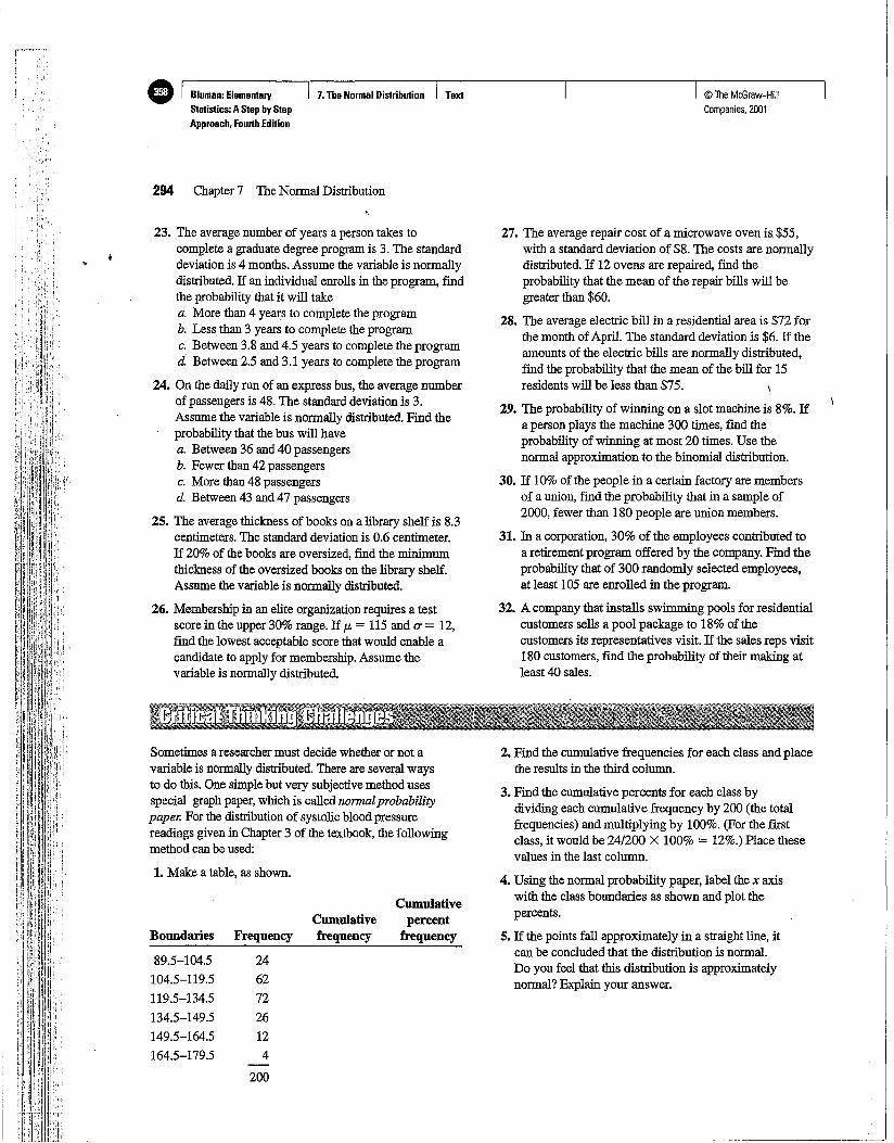
294 Chapter 7 The Normal Distribution
Sometimes a researcher must decide whether or not avariable is normally distributed. There are several waysto do this. One simple but very subjective method usesspecial graph paper, which is called normalprobabilitypaper. For the distribution of systolic blood pressurereadings given in Chapter 3 of the textbook, the followingmethod can be used:
4. Using the normal probability paper, label the x axiswith the class boundaries as shown and plot thepercents.
5. If the points fall approximately in a straight line, itcan be concluded that the distribution is normal.Do you feel that this distribution is approximatelynormal? Explain your answer.
© The McGraw-HiliCompanies, 2001
2. Find the cumulative frequencies for each class and placethe results in the third column.
3. Find the cumulative percents for each class bydividing each cumulative frequency by 200 (the totalfrequencies) and multiplying by 100%. (For the firstclass, it would be 24/200 X 100% = 12%.)Place thesevalues in the last column.
27. The average repair cost of a microwave oven is.$55,with a standard deviation of $8. The costs are normallydistributed. If 12 ovens are repaired, find theprobability that the mean of the repair bills will begreater than $60.
28. The average electric bill in a residential area is $72 forthe month of April. The standard deviation is $6. If theamounts of the electric bills are normally distributed,find the probability that the mean of the bill for 15residents will be less than $75.
29. The probability of winning on a slot machine is 8%. Ifa person plays the machine 300 times, find theprobability of winning at most 20 times. Use thenormal approximation to the binomial distribution.
30. If 10% of the people in a certain factory are membersof a union, find the probability that in a sample of2000, fewer than 180 people are union members.
31. In a corporation, 30% of the employees contributed toa retirement program offered by the company. Find theprobability that of 300 randomly selected employees,at least 105 are enrolled in the program.
32. A company that installs swimming pools for residentialcustomers sells a pool package to 18% of thecustomers its representatives visit. If the sales reps visit180 customers, find the probability of their making atleast 40 sales.
Cumulativepercent
frequency
7.TheNormal Distribution Text
Cumulativefrequency
1. Make a table, as shown.
23. The average number of years a person takes tocomplete a graduate degree program is 3. The standarddeviation is 4 months. Assume the variable is normallydistributed. If an individual enrolls in the program, findthe probability that it will takea. More than 4 years to complete the programb. Less than 3 years to complete the programc. Between 3.8 and 4.5 years to complete the programd. Between 2.5 and 3.1 years to complete the program
24. On the daily run of an express bus, the average numberof passengers is 48. The standard deviation is 3.Assume the variable is normally distributed. Find theprobability that the bus will havea. Between 36 and 40 passengersb. Fewer than 42 passengersc. More than 48 passengersd. Between 43 and 47 passengers
25. The average thickness of books on a library shelf is 8.3centimeters. The standard deviation is 0.6 centimeter.If 20% of the books are oversized, find the minimumthickness of the oversized books on the library shelf.Assume the variable is normally distributed.
26. Membership in an elite organization requires a testscore in the upper 30% range. If p., = 115 and (J' = 12,find the lowest acceptable score that would enable acandidate to apply for membership. Assume thevariable is normally distributed.
89.5-104.5 24
104.5-119.5 62
119.5-134.5 72
134.5-149.5 26
149.5-164.5 12
164.5-179.5 4
200
Boundaries Frequency
e Bluman: ElamentaryStatistics: AStep bV StepApproach, Fourth Edition
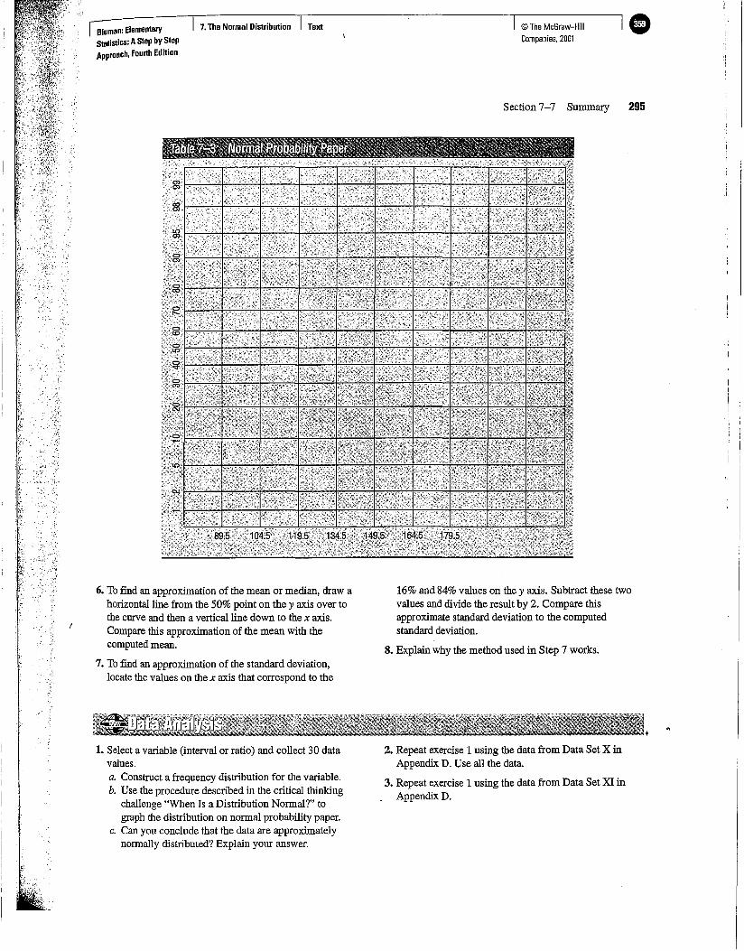
6. To find an approximation of the mean or median, draw ahorizontal line from the 50% point on the y axis over tothe curve and then a vertical line down to the x axis.Compare this approximation of the mean with thecomputed mean.
7. To fmd an approximation of the standard deviation,locate the values on the x axis that correspond to the
Section 7-7 Summary 295
© The McGraw-HiliCompanies. 2001
16% and 84% values on the y axis. Subtract these twovalues and divide the result by 2. Compare thisapproximate standard deviation to the computedstandard deviation.
8. Explain why the method used in Step 7 works.
2. Repeat exercise 1 using the data from Data Set X inAppendix D. Use all the data.
3. Repeat exercise 1 using the data from Data Set XI inAppendixD.
7.TheNormal Distribution TextBluman: ElementaryStatistics: AStepbyStepApproach, Fourth Edition
1. Select a variable (interval or ratio) and collect 30 datavalues.a. Construct a frequency distribution for the variable.b. Use the procedure described in the critical thinking
challenge "When Is a Distribution Normal?" tograph the distribution on normal probability paper.
c. Can you conclude that the data are approximatelynormally distributed? Explain your answer.
e BlumaR: ElementaryStatistics: AStep byStepApproach. Fourth Edition
B. Confidence Intervals and TextSample Size
© The McGrew-HiliCompanies, 2001
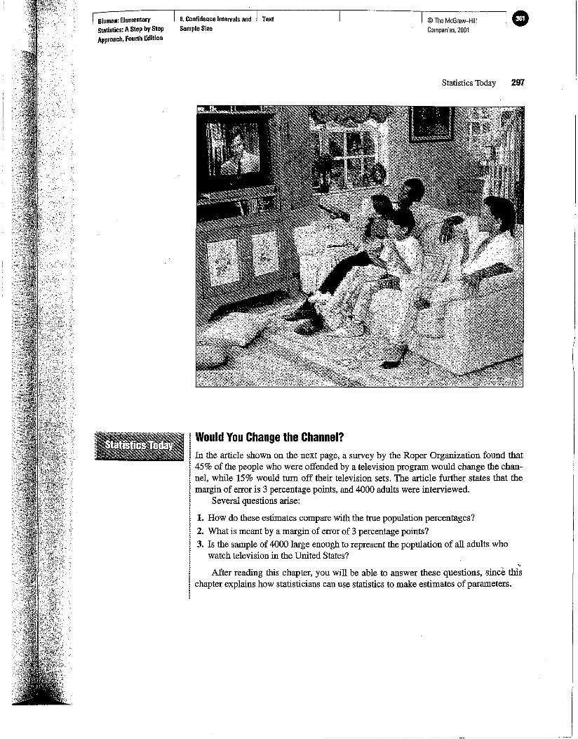
".After reading this chapter, you will be able to answer these questions, since this
chapter explains how statisticians can use statistics to make estimates of parameters.
In the article shown on the next page, a survey by the Roper Organization found that45% of the people who were offended by a television program would change the channel, while 15% would turn off their television sets. The article further states that themargin of error is 3 percentage points, and 4000 adults were interviewed.
Several questions arise:
1. How do these estimates compare with the true population percentages?
2. What is meant by a margin of error of 3 percentage points?
3. Is the sample of 4000 large enough to represent the population of all adults whowatch television in the United States?
Statistics Today 297
© The McGraw-HiliCompanies, 2001
Would You Change the Channel?
8.Confidence Intervals and TextSample Size
Bluman: ElementaryStatistics: A Step bVStepApproach, Fourth Edition
CD I 8luman: ElementaryStatistics: A Step byStepApproach. Fourth Edition
8.Confidence IntelVals and I TextSample Size
© The McGraw-HiliCompanies. 2001
298 Chapter 8 Confidence Intervals and Sample Size
TV Survey Eyes.On-Off Habitsspecial effort to watch shows they particularly like.
And despite increasing cable alternatives,about three-quarters of these "appointment"viewers with cable said that ABC, CBS andNBC still offer most of their favorites.
Viewers find TV news highly credible,the survey also said. In the event of conflicting news reports, 56 percent of respondentssaid they would believe television's accountabove others.
A hefty 69 percent said they get most oftheir news from TV. Newspapers were second, with 43 percent. Radio, word-of-mouthand magazines fell far behind.
A majority of the respondents reportedhaving seen something on television thatthey found "either personally offensive ormorally objectionable" in the past fewweeks. But only 42 percent could specifywhether it was profanity, sex or violence.
NEW YORK (AP)-You're watching TVand the show offends you. Do you sit thereand take it or do you get up and go?
A survey released yesterday on the public's attitudes toward television said 12 percent of the respondents do nothing, 45percent change channels and 15 percent turnoff their sets.
National Association of Broadcasters andthe Network Television Association, an alliance of the Big Three broadcast networks,co-sponsored the survey, which has beentaken every two years since 1959.
The Roper Organization polled 4,000adults nationwide in personal interviews between November and December last year.The results had a margin of sampling errorof plus or minus 3 percentage points.
The study, "America's Watching," saidthat even in an age of channel "grazing"about two in three viewers regularly make a
Source: Associated Press. Reprinted with permission,
"One out of4Americans is currently dieting." (Calorie Control Council. Used withpermission.)"Seventy-two percent ofAmericans haveflown in commercial airlines." ("The BristolMeyers Report: Medicine in the Next Century." Used with permission.)"The average kindergarten student has seen more than 5000 hours oftelevision." (U.S.Department ofEducation.)"The average school nurse makes $32,786 a year." (National Association ofSchoolNurses. Used with permission.)"The average amount oflife insurance is $108,000 per household with life insurance."(American Council ofLife Insurance. Used with permission.)
Since the populations from which these values were obtained are large, these valuesare only estimates of the true parameters and are derived from data collected from samples.
The statistical procedures for estimating the population mean, proportion, variance,and standard deviation will be explained in this chapter.
An important question in estimation is that of sample size. How large should thesample be in order to make an accurate estimate? This question is not easy to answersince the size of the sample depends on several factors, such as the accuracy desired andthe probability of making a correct estimate. The question of sample size will be explained in this chapter also.
One aspect of inferential statistics is estimation, which is the process of estimating thevalue of a parameter from information obtained from a sample. For example, The BookofOdds, by Michael D. Shook and Robert L. Shook (New York: Penguin Putnam, Inc.,1991), contains the following statements:
Introduction
© The McGraw-HiliCompanies, 2001
An interval estimate ofaparameter is an interval or arange of values used to estimate the parameter. Thisestimate mayor may not contain the value ofthe parameter being estimated.
In an interval estimate, the parameter is specified as being between two values.For example, an interval estimate for the average age of all students might be26.9 < JL < 27.7, or 27.3 ± 0.4 years.
Either the interval contains the parameter or it does not. A degree of confidence(usually a percent) can be assigned before an interval estimate is made. For instance,one may wish to be 95% confident that the interval contains the true population mean.Another question then arises. Why 95%? Why not 99% or 99.5%?
If one desires to be more confident, such as 99% or 99.5% confident, then the interval must be larger. For example, a 99% confidence interval for the mean age of
As stated in Chapter 7, the sample mean will be, for the most part, somewhat differentfrom the population mean due to sampling error. Therefore, one might ask a secondquestion: How good is a point estimate? The answer is that there is no way of knowinghow close the point estimate is to the population mean.
This answer places some doubt on the accuracy of point estimates. For this reason,statisticians prefer another type of estimate called an interval estimate.
Apoint estimate isaspecific numeric~ value estimate of aparameter. The best point estimate ofthepopulation mean t-t isthe sample mean X.
One might ask why other measures of central tendency, such as the median andmode, are not used to estimate the population mean. The reason is that the means ofsamples vary less than other statistics (such as medians and modes) when many samplesare selected from the same population. Therefore, the sample mean is the best estimateof the population mean.
Sample measures (i.e., statistics) are used to estimate population measures (i.e., parameters). These statistics are called estimators. As previously stated, the sample meanis a better estimator of the population mean than the sample median or sample mode.
A good estimator should satisfy the three properties described next.
Suppose a college president wishes to estimate the average age of the students attendingclasses this semester. The president could select a random sample of 100 students andfind the average age of these students, say 22.3 years. From the sample mean, the president could infer that the average age of all the students is 22.3 years. This type of estimate is called a point estimate.
Section 8-2 Confidence Intervals for the Mean (0' Known or n ~ 30) and Sample Size . 299
8.Confidence Intervals and TextSampleSize
Bluman: ElementaryStatistics: AStepbyStepAPproach, Fourth Edition
Confidence Intervalsfor the Mean (0'KnownDr n2: 30) and SampleSizeObjective 1. Find theconfidence interval forthemean when (T isknown orn2:30.
Confideru::e intervals
h_--------
e Bluman: ElementaryStatistics: AStepbyStepApproach, Fourth Edition
8.Confidence Intervals and TextSampleSize
© The McGraw-HiliCompanies. 2001
300 Chapter 8 Confidence Intervals and Sample Size
The confidence level ofan interval estimate of aparameter is the probability that the interval estimate willcontain the parameter.
Aconfidence interval isaspecific interval estimate ofaparameter determined by using data obtained fromasample and by using the specific confidence level ofthe estimate.
college students might be 26.7 < JL < 27.9, or 27.3 :±: 0.6. Hence, a trade-off occurs. Tobe more confident that the interval contains the true population mean, one must makethe interval wider.
Intervals constructed in this way are called confidence intervals. Three commonconfidence intervals are used: the 90%, the 95%, and the 99% confidence intervals.
The algebraic derivation of the formula for determining a confidence interval for amean will be shown later. A brief intuitive explanation will be given first.
The central limit theorem states that when the sample size is large, approximately95% of the sample means will fall within :±: 1.96 standard errors of the population mean.That is,
'Rointandinterv~l, '..........•.•·•.·.estjmates.were.known;a~i'.
~,~~lw~i.{t~~6E~··m~th~inatjCian·.Neym~n;fprmUIaf,
i,!praqlic~L?~pliqatt9il~i'iJhelTl. ;.,:;d"':;;~;,~.~-~ ~~~'~'~~:~ ..'~:'-~~'.;;~.-~.~'';~.''.~'~'~~ .
()6 :- ::'~) ,J!. c? ,_.')-~
JL :±: 1.96 .vn -;1 -.;.- ';; o "J'0...~ _....: "-Now, if a specific sample mean is selected, say X, there is a 95% probability that it fallswithin the range of JL :±: 1.96 (oo/Vii). Likewise, there is a 95% probability that the interval specified by
will contain JL, as will be shown later. Stated another way,
X - 1.96(.vn) < JL < X + 1.96( .vn)Hence, one can be 95% confident that the population mean is contained within that interval when the values of the variable are normally distributed in the population.
The value used for the 95% confidence interval, 1.96, is obtained from Table E in- Appendix C. For a 99% confidence interval, the value 2.58 is used instead of 1.96 in theformula. This value is also obtained from Table E and is based on the standard normaldistribution. Since other confIdence intervals are used in statistics, the symbol Za/2 (read
, "zee sub alpha over two") is used in the general formula for confidence intervals. TheGreek letter a (alpha) represents the total area in both of the tails of the standard normaldistribution curve. al2 represents the area in each one of the tails. More will be said af-ter Examples 8-1 and 8-2 about fmding other values for Za/2' .
The relationship between a and the confIdence level is that the stated confidence levelis the percentage equivalent to the decimal value of 1 - a, and vice versa. When the 95%confidence interval is to be found, a = 0.05, since 1 - 0.05 = 0.95, or 95%. When a =0.01, then 1 - a = 1 - 0.01 = 0.99, and the 99% confidence interval is being calculated.
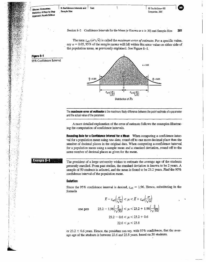
Section 8-2 Confidence Intervals for the Mean (0" Known or n ~ 30) and Sample Size 301
The maximum error ofestimate isthe maximum likely difference between the point estimate ofaparameterand the actual value of the parameter.
© The McGraw-HiliCompanies, 2001
lX =0.05
x- Za/2(Vn) < p, < X+ Za/2(Vn)
23.2 - 1.96(Jso) < P, < 23.2 + 1.96(Jso)23.2 - 0.6 < P, < 23.2 + 0.6
22.6 < P, < 23.8
one gets
The term Za/2 (ulyn) is called the maximum error ofestimate. For a specific value,say a = 0.05, 95% of the sample means will fall within this error value on either side ofthe population mean, as previously explained. See Figure 8-1.
ZlX/2(Ji) ZlX/2(Ji)Distribution ofXs
Amore detailed explanation of the error of estimate follows the examples illustrating the computation of confidence intervals.
Solution·
Since the 95% confidence interval is desired, Za/2 = 1.96. Hence, substituting in theformula
The president of a large university wishes to estimate the average age of the studentspresently enrolled. From past studies, the standard deviation is known to be 2 years. Asample of 50 students is selected, and the mean is found to be 23.2 years. Find the 95%confidence interval of the population mean.
Rounding Rule for a Confidence Interval for aMean When computing a confidence interval for a population mean using rawdata, round off to one more decimal place than thenumber of decimal places in the original data. When computing a confidence intervalfor a population mean using a sample mean and a standard deviation, round off to thesame number of decimal places as given for the mean.
8.Confidence Intervals and Text. Sample Size
Exampe~
95% Confidence Interval
Figure 8-1
. 8luman: ElementaryStatistics: AStep byStep
APproacb. Fourth Edition
or 23.2 ± 0.6 years. Hence, the president can say, with 95% confidence, that the average age of the students is between 22.6 and 23.8 years, based on 50 students.
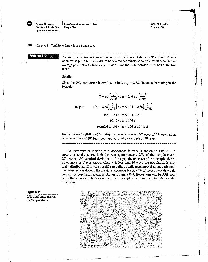
e I Blumen: ElementaryStatistics:AStepby StepApproach. Fourth Edition
I 8.Confidence Intervels and , TextSampleSize
© The McGraw-HiliCompanies, 2001
302 Chapter 8 Confidence Intervals and Sample Size
Solution
Since the 99% confidence interval is desired, Za/Z = 2.58. Hence, substituting in theformula
x - Za/Z(.;n) <!J- < X+ Za/Z(.;n)
104 - 2.58(Jo) <!J- < 104 + 2.58(Jo)
104 - 2.4 < !J- < 104 + 2.4
101.6 < !J- < 106.4
rounded to 102 <!J- < 106 or 104 ± 2
one gets
A certain medication is known to increase the pulse rate of its users. The standard deviation of the pulse rate is known to be 5 beats per minute. A sample of 30 users had anaverage pulse rate of 104 beats per minute. Find the 99% confidence interval of the truemean.
Hence one can be 99% confident that the mean pulse rate of all users of this medicationis between 102 and 106 beats per minute, based on a sample of 30 users.
Another way of looking at a confidence interval is shown in Figure 8-2.According to the central limit theorem, approximately 95% of the sample meansfall within 1.96 standard deviations of the population mean if the sample size is30 or more or if (T is known when n is less than 30 when the population is normally distributed. If it were possible to build a confidence interval about each sample mean, as was done in the previous examples for !J-, 95% of these intervals wouldcontain the population mean, as shown in Figure 8-3. Hence, one can be 95% confident that an interval built around a specific sample mean would contain the population mean.
Figure 8-295% Confidence Intervalfor Sample Means

95% Confidence Intervalsfor Each Sample Mean
Section 8-2 Confidence Intervals for the Mean (0' Known or n ~ 30) and Sample Size 303
© The McGraw-HiliCompanies, 2001
Ifone desires to be 99% confident, the confidence intervals must be enlarged so that 99out of every 100 intervals contain the population mean.
Since other confidence intervals (besides 90%, 95%, and 99%) are sometimes usedin statistics, an explanation of how to find the values for Zctl2 is necessary. As statedpreviously, the Greek letter IX represents the total of the areas in both tails of the normaldistribution. The value for IX is found by subtracting the decimal equivalent for the desired confidence level from 1. For example, if one wanted to find the 98% confidenceinterval, one would change 98% to 0.98 and find IX = 1 - 0.98, or 0.02. Then al2 isobtained by dividing IX by 2. So al2 is 0.02/2, or 0.01. Finally, Zo.01 is the z value thatwill give an area of 0.01 in the right tail of the standard normal distribution curve. SeeFigure 8-4.
Once al2 is determined, the corresponding Zctl2 value can be found by using the procedure shown in Chapter 7 (see Example 7-17), which is reviewed here. To get the Zctl2
value for a 98% confidence interval, subtract 0.01 from 0.5000 to get 0.4900. Next,
8.Confidence Intervals and TextSample Size
Bluman: ElementaryStatistics: AStep byStepApproach, Fourth Edition
Figure 8-3
Finding al2 for a 98%Confidence Interval
Figure 8-4

•
304 Chapter 8 Confidence Intervals and Sample Size
locate the area that is closest to 0.4900 (in this case, 0.4901) in Table E, and then [rodthe corresponding z value. In this example, it is 2.33. See Figure 8-5.
© The McGraw-HiliCompanies. 2001
I 8.Confidence Intervals and I TextSampleSize
For confidence intervals, only the positive zvalue is used in the formula.When the original variable is normally distributed and a is known, the standard
normal distribution can be used to find confidence intervals regardless of the size of thesample. When n ~ 30, the distribution of means will be approximately normal even ifthe original distribution of the variable departs from normality. Also, ifn =::: 30 (someauthors use n > 30), S can be substituted for ain the formula for confidence intervals;and the standard normal distribution can be used to find confidence intervals for means,as shown in the next example.
Finding Za/2 for a 98%Confidence Interval
Figure 8-5
e I Bluman: ElamentBryStatistics:AStepbyStepApproach. Fourth Edition
"
I I'?,'F"''-
, Example 1E3 The following data represent a sample of the assets (in millions of dollars) of 30 creditunions in Southwestern Pennsylvania. Find the 90% confidence interva1 of the mean.
$12.23
2.89
13.1973.25
11.59
8.74
7.92
40.22
5.01
2.27
$16.56
1.24
9.16
1.91
6.69
3.17
4.78
2.42
1.47
12.77
$ 4.39
2.17
1.42
14.64
1.06
18.13
16.85
21.58
12.24
2.76
Source: Pittsburgh Post Gazette, June 7, 1998.
Solution:
STEP 1 Find the mean and standard deviation for the data. Use the formulas shownin Chapter 3 or your calculator. The mean X = 11.091.The standard deviation s = -14.405.
STEP 2 Find al2. Since the 90% confidence interval is to be used, a = 1 - 0.90= 0.10, and
~ = 0.;0 = 0.05
Section 8-2 Confidence Intervals for the Mean (0' Known or n ~ 30) and Sample Size 305
yn = Zei/2' (T
E
©The McGraw-HiliCompanies. 2001
STEP 3 Find Zei!2' Subtract 0.05 from 0.5000 to get 0.4500. The corresponding Z
value obtained from Table E is 1.65. (Note: This value is found by using theZ value for an area between 0.4495 and 0.4505. Amore precise Z valueobtained mathematically is 1.645 and is sometimes used; however, 1.65 willbe used in this textbook.)
STEP 4 Substitute in the formula
JI- Zri/2(Vn) < JL < JI+ Zri/2(Vn)
(s is used in place of (T when (Tis unknown, since n 2:: 30.)
(14.405) (14.405)11.091 - 1.65 yI30 < JL < 11.091 + 1.65 V30
11.091 - 4.339 < JL < 11.091 + 4.339
6.752 < JL < 15.430
Hence, one can be 90% confident that the population mean of the assets of all creditunions is between $6.752 million and $15.430 million, based on a sample of 30 creditunions.
Sample size determination is closely related to statistical estimation. Quite often, one asks,''How large a sample is necessary to make an accurate estimate?" The answer is not simple, since it depends on three things: the maximum error of estimate, the population standard deviation, and the degree of confidence. For example, how close to the true meandoes one want to be (2 units, 5 units, etc.), and how confident does one wish to be (90%,95%,99%, etc.)? For the purpose of this chapter, it will be assumed that the populationstandard deviation of the variable is known or has been estimated from a previous study.
The formula for sample size is derived from the maximum error of estimateformula,
E = ZeiI2(V"n)
and this formula is solved for n as follows:
Eyn = Zri/z{(T)
8.Confidence IntelVals and TextSample Size
Bluman: ElementaryStatistics: AStep by StepApproach. Fourth Edition
Sample SizeObjective 2, Determine theminimum sample size forfinding aconfidence intervalforthe mean.
Hence,

o Bluman: ElemantBryStatistics: A Step byStepApproach. Fourth Edition
8.Confidence Intervals and TextSample Size
© The McGraw-HiliCompanies. 2001
-
306 Chapter 8 Confidence Intervals and Sample Size
. Example H .' The college president asks the statistics teacher to estimate the average age of the students at their college. How large a sample is necessary? The statistics teacher would liketo be 99% confident that the estimate should be accurate within one year. From a previous study, the standard deviation of the ages is known to be 3 years.
Solution
Since a = 0.01 (or 1 - 0.99), Za/2 = 2.58, and E = 1, substituting in the formula,one gets
n = (Zcrlk O'f = [(2.5~)(3)r = 59.9
which is rounded up to 60. Therefore, in order to be 99% confident that the estimateis within 1 year of the true mean age, the teacher needs a sample size of at least 60students.
Notice that when one is finding the sample size, the size of the population is irrelevant when the population is large or infinite or when sampling is done with replacement.In other cases, an adjustment is made in the formula for computing sample size. This adjustment is beyond the scope of this book.
The formula for determining sample size requires the use of the population standarddeviation. What then happens when 0' is unknown? In this case, an attempt is made toestimate 0'. One such way is to use the standard deviation, S, obtained from a sampletaken previously as an estimate for 0'. The standard deviation can also be estimated bydividing the range by 4.
Sometimes, interval estimates rather than point estimates are reported. For instance,one may read a statement such as "On the basis of a sample of 200 families, the surveyestimates that an American family of two spends an average of $84 per week for groceries. One can be 95% confident that this estimate is accurate within $3 of the truemean." This statement means that the 95% confidence interval of the true mean is
$84 - $3 < JL < $84 + $3
$81 < JL < $87
The algebraic derivation of the formula for a confidence interval is shown next. Asexplained in Chapter 7, the sampling distribution of the mean is approximately normalwhen large samples (n ~ 30) are taken from a population. Also,
X-JLz=--u/vn
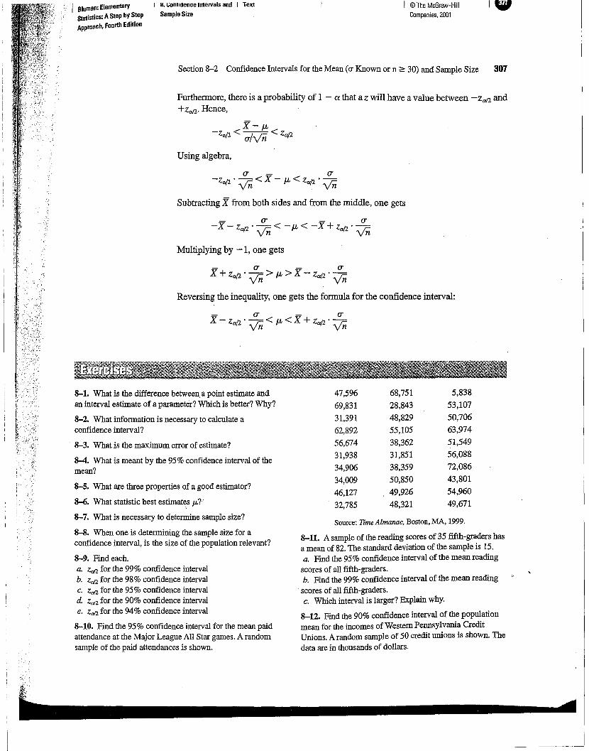
Section 8-2 Confidence Intervals for the Mean (0' Known or n ze 30) and Sample Size 307
Furthermore, there is a probability of 1 - a that a Z will have a value between -ZaJ2 and+ZaJ2' Hence,
5,838
53,107
50,706
63,974
51,549
56,088
72,086
43,801
54,960
49,671
© The McGraw-HiliCompanies. 2001
68,751
28,843
48,829
55,105
38,362
31,851
38,359
50,850
49,926
48,321
47,596
69,831
31,391
62,892
56,674
31,938
34,906
34,009
46,127
32,785
Source: Time Almanac, Boston, MA, 1999.
8-11. A sample of the reading scores of 35 fifth-graders hasa mean of 82. The standard deviation of the sample is 15.a. Find the 95% confidence interval of the mean reading
scores of all fifth-graders.b. Find the 99% confidence interval of the mean reading
scores of all fifth-graders.c. Which interval is larger? Explain why.
8-12. Find the 90% confidence interval of the populationmean for the incomes of Western Pennsylvania CreditUnions. A random sample of 50 credit unions is shown. Thedata are in thousands of dollars.
X-/-L- Za/2 < cr/Vii < Za/2
Using algebra,
- cr - UX+Za/2' Vii> /-L>X-Za/2' vn
Reversing the inequality, one gets the formula for the confidence interval:
u - U-Za/2' Vii<X- /-L<Za/2' vn
Subtracting Xfrom both sides and from the middle, one gets
- u - u-X - Za/2' Vii < -/-L < -X + Za/2 . Vii
Multiplying by -1, one gets
I II. connaence Intervals and I Text
Sample Size
8-1. What is the difference between a point estimate andan interval estimate of a parameter? Which is better? Why?
8-2. What information is necessary to calculate aconfidence interval?
8-3. What is the maximum error of estimate?
8-4. What is meant by the 95% confidence interval of themean?
8-5. What are three properties of a good estimator?
8-6. What statistic best estimat~s J.L?""
8-7. What is necessary to determine sample size?
8-8. When one is determining the sample size for aconfidence interval, is the size of the population relevant?
8-9. Find each.a. Za/2for the 99% confidence intervalb. Za/2for the 98% confidence intervalc. Za/2for the 95% confidence intervald. ZcJ2for the 90% confidence intervale. ZcJ2for the 94% confidence interval
8-10. Find the 95% confidence interval for the mean paidattendance at the Major League AIl Star games. A randomsample of the paid attendances is shown.
I BlumBn: ElementaryStatistics: A Step byStepAppfDBCh, FDurth EditiDn
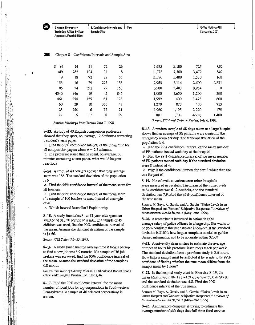
Source: Pittsburgh Post Gazette, June 7, 1998.
308 Chapter 8 Confidence Intervals and Sample Size
©TheMcGraw-HiliCompanies, 2001
7,685 3,100 725 850
11,778 7,300 3,472 540
11,370 5,400 1,570 160
9,953 3,114 2,600 2,821
6,200 3,483 8,954 8
1,000 1,650 1,200 390
1,999 400 3,473 600
1,270 873 400 713
11,960 1,195 2,290 175
887 1,703 4,236 1,400
Source: PittsburghTribuneReview, July 6, 1997.
8-18. A random sample of 48 days taken at a large hospitalshows that an average of 38 patients were treated in theemergency room per day. The standard deviation of thepopulation is 4.a. Find the 99% confidence interval of the mean numberof ER patients treated each day at the hospital.b. Find the 99% confidence interval of the mean number
of ER patients treated each day if the standard deviationwere 8 instead of 4.c. Why is the confidence interval for part b wider than the
one for part a?
8-19. Noise levels at various area urban hospitalswere measured in decibels. The mean of the noise levelsin 84 corridors was 61.2 decibels, and the standarddeviation was 7.9. Find the 95% confidence interval ofthe true mean.
Source: M. Bayo, A. Garcia, and A. Garcia, "Noise Levels in anUrban Hospital and Workers' Subjective Responses," Archives ofEnvironmental Health50, no. 3 (May-June 1995).
8-20. A researcher is interested in estimating theaverage salary of police officers in a large city. She wants tobe 95% confident that her estimate is correct. If the standarddeviation is $1050, how large a sample is needed to get thedesired information and to be accurate within $200?
8-21. A university dean wishes to estimate the averagenumber of hours his part-time instructors teach per week.The standard deviation from a previous study is 2.6 hours.How large a sample must be selected ifhe wants to be 99%confident of finding whether the true mean differs from thesample mean by 1 hour?
8-22. In the hospital study cited in Exercise 8-19, themean noise level in the 171 ward areas was 58.0 decibels,and the standard deviation was 4.8. Find the 90%confidence interval of the true mean.
Source: M. Bayo, A. Garcia, and A. Garcia, "Noise Levels in anUrban Hospital and Workers' Subjective Responses," Archives ofEnvironmentalHealth50, no. 3 (May-June 1995).
8-23. An insurance company is trying to estimate theaverage number of sick days that full-time food-service
8.Confidence IntelVals and I TextSample Size
$ 84 14 31 72 26
;49 252 104 31 8
3 18 72 23 55
133 16 29 225 138
85 24 391 72 158
4340 346 19 5 846
461 254 125 61 123
60 29 10 366 47
28 254 6 77 21
97 6 17 8 82
8-13. A study of 40 English composition professorsshowed that they spent, on average, 12.6 minutes correctinga student's term paper.a. Find the 90% confidence interval of the mean time for
all composition papers when a = 2.5 minutes.b. If a professor stated that he spent, on average, 30
minutes correcting a term paper, what would be yourreaction?
8-16. A study found that the average time it took a personto find a new job was 5.9 months. If a sample of 36 jobseekers was surveyed, find the 95% confidence interval ofthe mean. Assume the standard deviation of the sample is0.8 month.
Source: The Book ofOddsby Michael D. Shook and Robert Shook(New York: Penguin Putnam, Inc., 1991),46.
8-17. Find the 90% confidence interval for the meannumber of local jobs for top corporations in SouthwesternPennsylvania. A sample of 40 selected corporations isshown.
8-14. A study of 40 bowlers showed that their averagescore was 186. The standard deviation of the populationis 6.a. Find the 95% confidence interval of the mean score forall bowlers.b. Find the 95% confidence interval of the mean scoreif a sample of 100 bowlers is used instead of a sampleof 40.c. Which interval is smaller? Explain why.
8-15. A study found that 8- to 12-year-olds spend anaverage of $18.50 per trip to a mall. If a sample of 49children was used, find the 90% confidence interval ofthe mean. Assume the standard deviation of the sampleis $1.56.
Source: USA Today, July 25, 1995.
o I 8luman: ElementaryStatistics: AStep byStepApproach, Fourth Edition
..

4425 2620
1919
95·;~·ift~ 1:1'.2Jft~ ]l~#91lJ
© The McGraw-HiliCompanies, 2001
24 3236 47
42 3227 33
;;t()efM HE" t;~t1:;£U'],
1.11- .• til. 2:;..111
2121
4323
accurate within $0.1O?A previous study showed that thestandard deviation of the price was $0.12.
8-25. A health care professional wishes to estimate thebirth weights of infants. How large a sample must sheselect if she desires to be 90% confident that the true meanis within 6 ounces of the sample mean? The standarddeviation of the birth weights is known to be 8 ounces.
4525
25
2218 20
41 53
~,QU~tiillJlrl
);1
0t1'Il·S;f'l;mpIEl·:Z~C'111n,et~s:~'lJtJ!j,c;.jj, !11'~~~ ~ .it
5. Click the [Options] button. In the dialog box make sure the Confidence Level is95.0 (in Release 12 the Confidence Level is set in the I-Sample Z dialog box, withoutclicking Options). You may need to click inside the textbox before you type the new level.
6. Click [OK].
The results will be displayed in the session window.
1. Enter the data into C1 of a MINITAB worksheet.
2. Select Stat>Basic Statistics>1-Sample Z.
3. Select C1 for the variable.
4. Click in the box for Sigma and enter 11.If the standard deviation for the population wereunknown, you would calculate the standard deviation for the sample and use s.
43 52
42 41
Example MT8-1Find the 95% confidence interval when (J' = 11 using the following sample:
Section 8-2 Confidence Intervals for the Mean «J' Known or n ;;::: 30) and Sample Size 309
8.Confidence lntervals and TextSampleSize
Session Window with .Z-Interval
l-Sample Z Dialog Box
MINITABStep by Step
workers use per year. A pilot study found the standarddeviation to be 2.5 days. How large a sample must beselected if the company wants to be 95% confident ofgetting an interval that contains the true mean with a
maximum error of 1 day?
8-24. A restaurant owner wishes to find the 99%confidence interval of the true mean cost of a dry martini.HoWlarge should the sample be if she wishes to be
8luman: ElementaryStatistics: AStepbyStepApproach, Fourth Edition
s.....

•
For confidence intervals, the calculator will accept either raw data or summary statistics.
]Ei'imli1Em~ a it Ci[j)mrl1d~!flJ.~ mrerwaH f®Ir tlhl~ MelEu!ll (Sbl&tics)1. Press STAT and move the cursor to TESTS.2. Press 7.
3. Select Stats and press ENTER. Move cursor to 0".
4. Enter the value for the population standard deviation, 0".
5. Enter the sample mean, X.6. Enter the sample size.
7. Type in the correct confidence level.
8. Select Calculate and press ENTER.
1316
© The McGraw-HiliCompanies. 2001
1816
ZInterval"1'-' "":'1.... .-, ..... 4°"')1;• .£..( .::..,..::.....:... ~I(
x=17.6Sx=6.818276094n=10
•
15321491627
ZInter'valInpt.:I~ Stats.,.:6List:L1Freo:.t:1C-Le....'e 1: •99Calculate
8.Confidence Intervalsand TextSample Size
IF'fjWJi!lii~ ~l Z C\Q)!lllft!1itll{t:;]j'll~ Th.rll11Jell'w~R mt!JI£' tlfu.1e JWJ(~lm (IDF;dlt-my1. Enter the data into L1.
2. Press STAT and move the cursor to TESTS.3. Press 7.
4. Select Data, and press ENTER and move cursor to 0".
5. Enter the values for 0". Make sure L1 is selected and Freq is 1.
6. Type in the correct confidence level.
7. Select Calculate and press ENTER.
Example TIS-IFind the 99% confidence interval for the mean when 0" = 6 using the following data:
E1<iiLlI!!!llpnfJ 1['][8=2
Find the 90% confidence interval of the mean when X = 182, 0" = 8, and n =50.
Input Output
ZInterval ZIntervalInpt:Oata ~~ (180.14,183.86).,.:8 x=182x: 182 n=50n:50C-Le...)e1: • 9Calculate
TI-83Step by Step
310 Chapter 8 Confidence Intervals and Sample Size
CD 8luman:ElementaryStatistics:A Step byStepApproach. Fourth Edition
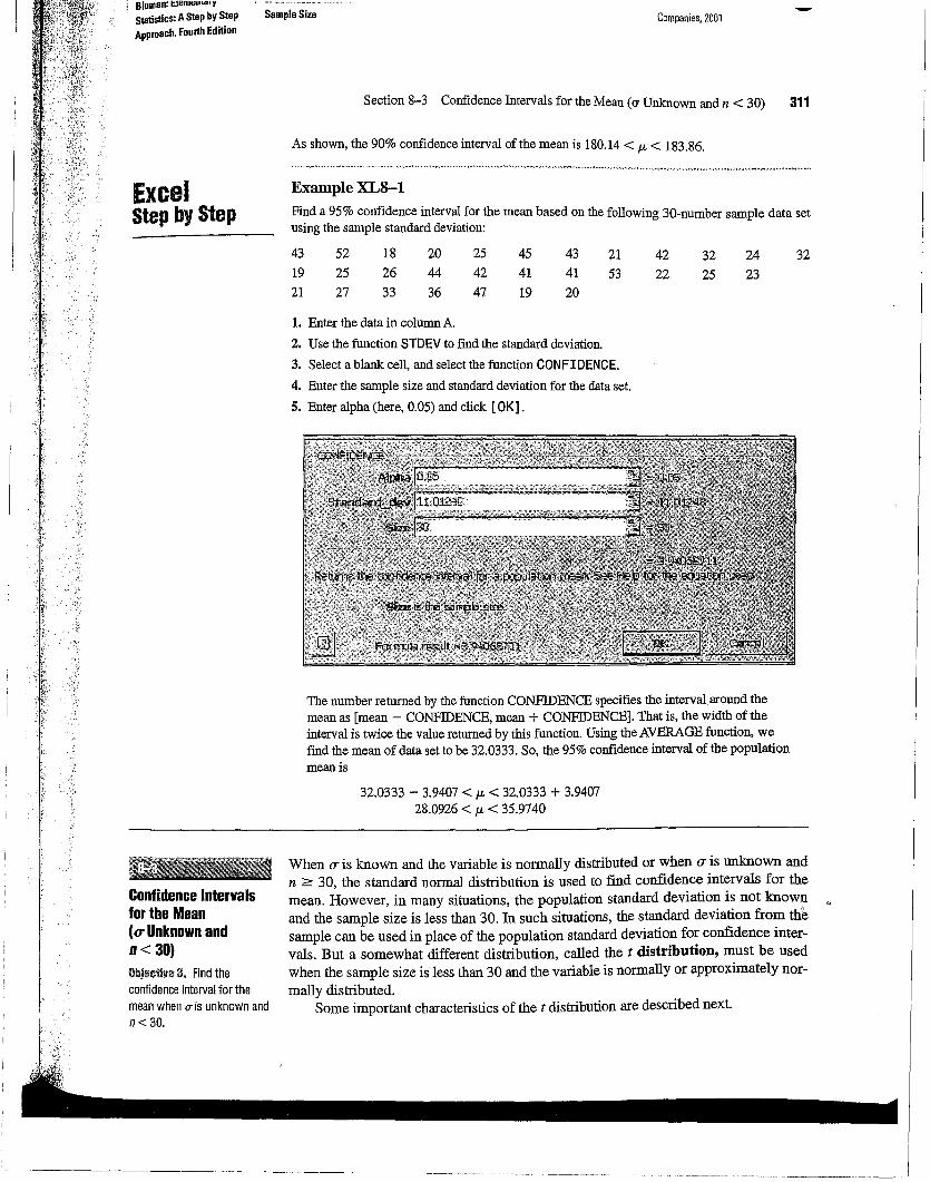
Example XL8-1Find a 95% confidence interval for the mean based on the following 3D-number sample data setusing the sample standard deviation:
3224
23
32
25
Companies, 2001
42
22
21
53
43
41
20
45
41
19
25
42
47
20
44
36
18
26
33
Section 8-3 Confidence Intervals for the Mean (0" Unknown and n < 30) 311
52
25
27
32.0333 - 3.9407 < JL < 32.0333 + 3.940728.0926 < JL < 35.9740
The number returned by the function CONFIDENCE specifies the interval around themean as [mean - CONFIDENCE, mean + CONFIDENCE]. That is, the width of theinterval is twice the value returned by this function. Using the AVERAGE function, wefind the mean of data set to be 32.0333. So, the 95% confidence interval of the populationmean is
As shown, the 90% confidence interval of the mean is 180.14 < JL < 183.86.
43
19
21
1. Enter the data in column A.
2. Use the function STDEV to find the standard deviation.
3. Select a blank cell, and select the function CONFIDENCE.
4. Enter the sample size and standard deviation for the data set.
5. Enter alpha (here, 0.05) and click [OK].
When (T is known and the variable is normally distributed or when (T is unknown andn 2': 30, the standard normal distribution is used to find confidence intervals for themean. However, in many situations, the population standard deviation is not knownand the sample size is less than 30. In such situations, the standard deviation from thesample can be used in place of the population standard deviation for confidence intervals. But a somewhat different distribution, called the t distribution, must be usedwhen the sample size is less than 30 and the variable is normally or approximately normally distributed.
Some important characteristics of the t distribution are described next.
Sample Size
ExcelStep by Step
Confidence Intervalsfor the Mean(u Unknown andn< 3D)~l3jeciille 3. Find theconfidence interval for themean when o:isunknown andn« 30.
I Siuman: tlem."'....J
Statistics: AStepbyStepApproach, Fourth Edition

CD Bluman: ElementaryStatistics:AStepbyStepApproach, Fourth Edition
8.Confidence Intervals Bnd TextSampleSize
© The McGraw-HiliCompanies, 2001
312 Chapter 8 Confidence Intervals and Sample Size
,Tlletdistrlbutionwas;'forrnulated;in.1.908'gY'an. .j.
:lris~"breVl'iQg·.ernpIOye~::•• \nameitw.s~G()sset."':;'
~~~t~i~~li;J,Bscause:b!:iernployea:';~l{()~ed,to;p~bl}Gpssetpllplish':;fihdinQ~lli6gt .
Figure 8-6 zThe t Familyof Curves
o
Many statistical distributions use the concept of degrees of freedom, and the formulas for fmding the degrees of freedom vary for different statistical tests. The degreesof freedom are the number of values that are free to vary after a sample statistic hasbeen computed, and they tell the researcher which specific curve to use when a distribution consists of a family of curves.
For example, if the mean of 5 values is 10, then 4 of the 5 values are free to vary.But once 4 values are selected, the fifth value must be a specific number to get a sum of50, since 50 -;- 5 = 10. Hence, the degrees offreedom are 5 - 1 = 4, and this value tellsthe researcher which t curve to use.
The symbol d.f. will be used for degrees of freedom. The degrees of freedom for aconfidence interval for the mean are found by subtracting 1 from the sample size. Thatis, d.f. = n - 1.Note: For some statistical tests used later in this book, the degrees offreedom are not equal to n - 1.
The formula for fmding a confidence interval about the mean using the t distribution is given next.
----" .------_._- .. ---------------_._----._------------------------'

© 1he McGraw-Hi IIcompanies, 1001
x- ta/2(0z) < JL < X+ ta/2k~n)
Hence, 0.32 - (2.262}(~) < JL < 0.32 + (2.26Z)(~)0.32 - 0.057 < JL < 0.32 + 0.051
0.26 < JL < 0.38
Therefore, one can be 95% confident that the populationmean tr~ad depthof all rightfront tires is between 0.26 and 0.38 inch based on a sample of 10ores.
Tenrandomly selected automobiles were stopped, and the tread depth ofthe right fronttire was measured. The mean was 0.32 inch, and the standard deviation was 0.08 inch.Find the 95% confidence interval of the mean depth. Assume that the variable is ap-
proximately normally distributed.
SolutionSince c is unknown and s must replace it, the t distribution (Table F) mustbe used for
95%. Hence, with 9 degrees of freedom, tal2 = 2.262.The 95% confidenceinterval of the populationmeanis foundby substituting in the
formula
.............................................................................................................................................................................
Note: At the bottom of Table F where d.f, =00, the Za/2 valuescan befound for specific confidence intervals. The reason is that as the degrees of freedom increase, the t
distribution approaches the standard normal distribution.The next two examples show how to find theconfidenceinterval when one is using
the t distribution.
Section 8-3 Confidence Intervals for the Mean ((J' UnJOl0wn and n < 30) 313
d.f = 22 - 1, or 21. Find 21 in the left columnand95% in the roW labeled "ConfidenceIntervals." The intersection where the two meet gives the value for taf)., whichis 2.080.
SeeFigure 8-7.
Thevaluesfor tcJ2 arefoundin TableF inAppendix C.Thetop roW ofTable F, labeled"Confidence Intervals,"is used to get thesevalues. Theothertwo rows, labeled "One Tail"and''TwoTails," will be explainedin the nextchapterandshouldnot be used here.
The next example shows how to find the valuein Table F for taf).'
F;d"ili~'~~~'~'~~~'f~;'~'95'%'~~;d~~~~';~~;~';h~~'ili;';;;~1~'~i~~'i·~"22:·"""··"""""··
Solution
8.Confidence Intervals and TextSample Size
Ii" ",e "
a·population,of: " ,'rcerateci criminals. For, ,
easures:heusedthe, !.,:thscif.cmB ciftheir ,.;ern.'" ", ,,>~. ~~~~~.~~'.'~~~'.;:-~~:,i·~~~'~~~ ~~::'~~~'i ~'. ~~..
EXample &-5
Finding tanforExample 8-5
Figure 8-7
Bluman:ElementaryStatistics: A Step byStepApproach.Fourth Edition
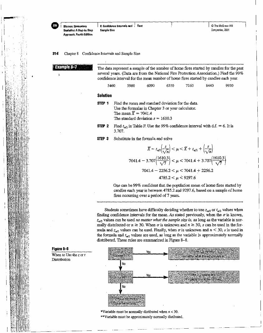
9930
© The McGraw-HiliCompanies. 2001
8440716063106090
Yes
Yes
Text
59005460
8.Confidence IntervalsandSample Size
'...............................................................................................................................................................................
Solution
STEP 1 Find the mean and standard deviation for the data.Use the formulas in Chapter 3 or your calculator.The mean X = 7041.4The standard deviation s = 1610.3
STEP 2 Find ta/2 in Table F.Use the 99% confIdence interval with d.f. = 6. It is3.707.
*Variable must be normally distibuted when n < 30.
**Variable must be approximately normally distibuted.
The data represent a sample of the number of home fires started by candles for the pastseveral years. (Data are from the National Fire Protection Association.) Find the 99%confIdence interval for the mean number of home fires started by candles each year.
STEP 3 Substitute in the formula and solve
X - ta/2(Jn) < /L< X + ta/2 + (In)7041.4 - 3.707(1~3) < /L < 7041.4 + 3.707(1~3)
7041.4 - 2256.2 < /L < 7041.4 + 2256.2
4785.2 < /L <: 9297.6
One can be 99% confIdent that the population mean of home fires started bycandles each year is between 4785.2 and 9297.6, based on a sample of homefires occurring over a period of 7 years.
Students sometimes have difficulty deciding whether to use Zal2 or ta/2 values whenfinding confidence intervals for the mean. As stated previously, when the (J'is known,Zal2 values can be used no matter what the sample size is, as long as the variable is normally distributed or n === 30. When (J'is unknown and n === 30, s can be used in the formula and Za/2 values can be used. Finally, when rr is unknown and n < 30, s is used inthe formula and tal2values are used, as long as the variable is approximately normallydistributed. These rules are summarized in Figure 8-8.
Bluman: ElementaryStatistics: AStep bVStepApproach. Fourth Edition
;,
Exampe ' 7
314 Chapter 8 Confidence Intervals and Sample Size
When to Use the zor tDistribution
Figure s-a
"
I

I(l:1"I
.,i'
"
$55$60$55
©The McGraw-HiliCompanies, 2001
$55 $70$60 $56 $60
Source: Pittsburgh Tribune Review, November 30, 1997.
8-37. A recent study of 28 city residents showed that themean of the time they had lived at their present address was9.3 years. The standard deviation of the sample was 2years. Find the 90% confidence interval of the true mean.
8-38. An automobile shop manager timed six employeesand found that the average time it took them to change awater pump was 18 minutes. The standard deviation of thesample was 3 minutes. Find the 99% confidence interval ofthe true mean.
8-39. A recent study of 25 students showed that they spentan average of $18.53 for gasoline per week. The standarddeviation of the sample was $3.00. Find the.95%confidence interval of the true mean.
8-40. For a group of 10 men subjected to a stress situation,the mean number of heartbeats per minute was 126, and the,standard deviation was 4. Find the 95% confidence interval
of the true mean.
8-41. For the stress test described in Exercise 8-40, sixwomen had an average heart rate of 115 beats per minute.The standard deviation of the sample was 6 beats. Find the95% confidence interval of the true mean for the women.
8-42. For a sample of 24 operating rooms taken in thehospital study mentioned in Exercise 8-19" ~e ~ean noiselevel was 41.6 decibels, and the standard deviation was 7.5.Find the 95% confidence interval of the true mean of thenoise levels in the operating rooms.Source: M. Bayo, A. Garcia, and A. Garcia, ''Noise Levels in anUrban Hospital and Workers' Subjective Responses," ArchivesofEnvironmental Health 50, no. 3 (May-June 1995).
8-43. Find the 98% confidence interval of the meantaxable assessed values for the City of Pittsburgh. Arandom sample of 14 wards is shown. Data are in millions
the sample was 1.6. Find the 90% confidence interval of thetrue mean.
8-35. A sample of 6 adult elephants had an average weightof 12,200 pounds, with a sample standard deviation of 200pounds. Find the 95% confidence interval of the true mean.
8-36. The daily salaries of substitute teachers for 8 localschool districts is shown. What is the point estimate for themean? Find the 90% confidence interval of the mean forthe salaries of substitute teachers in the region.
Section 8-3 Confidence Intervals for the Mean ((J' Unknown and n < 30) 315
It should be pointed out that some statisticians have a different point of view. Theyuse Zal2 values when o is known and tal2 values when o is unknown. In these circumstances, a t table that contains t values for sample sizes greater than or equal to 30 wouldbe needed. The procedure shown in Figure 8-8 is the one used throughout this textbook.
8.Confidence Intervals and TextSample Size ,
Bluman:ElementaryStatistics: AStep byStepApproach, Fourth Edition
5 33 35 37 24
31 16 45 19 13
18 29 15 39 18
58 132
8-34. A sample of 20 tuna showed that they swim anaverage of 8.6 miles per hour. The standard deviation for
8-26. What are the properties of the t distribution?
8-27. Who developed the t distribution?
8-28. What is meant by degrees of freedom?
8-29. When should the t distribution be used to find aconfidence interval for the mean?
8-30. (ans) Find the values for each.a. tal2 and n = 18 for the 99% confidence interval for
the meanb. tal2 and n = 23 for the 95% confidence interval for
the meanc. tal2 and n = 15 for the 98% confidence interval for
the meand. tal2 and n = 10 for the 90% confidence interval for
the meane. tal2 and n = 20 for the 95% confidence interval for
the mean
For Exercises 8-31 through 8-46, assume that allvariables are approximately normally distributed.
8-31. The average hemoglobin reading for a sample of 20teachers was 16 grams per 100 milliliters, with a samplestandard deviation of 2 grams. Find the 99% confidenceinterval of the true mean.
8-32. A meteorologist who sampled 15 cold weather frontsfound that the average speed at which they traveled across acertain state was 18 miles per hour. The standard deviationof the sample was 2 miles per hour. Find the 95%confidence interval of the mean.
8-33. A state representative wishes to estimate the meannumber of women representatives per state legislature. Arandom sample of 17 states is selected, and the number ofwomen representatives is shown below. Based on thesample, what is the point estimate of the mean? Find the90% confidence interval of the mean population. (Note: Thepopulation mean is actually 31.72 or about 32.) Comparethis value to the point estimate and the confidence interval.There is something unusual about the data. Describe it andstate how it would affect the confidence interval.
------~--'-'----------~---'------ I
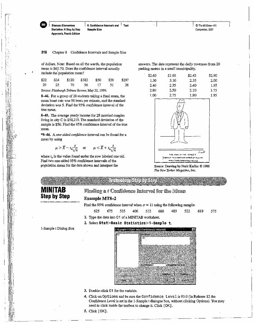
575
TME MAN IN i}ol( ~TRE£T
()\lI5'1l'tT TOA ~PLINc;.I"Uloll0'" PLUS Oil.
"'1"'V~ TMUE 1£«(N1.&( CIo'JolTS)
.J...J-
© The McGraw-HiliCompanies, 2001
Source: Drawing by Nurit Karlin: © 1988The New YorkerMagazine, Inc.
$2.60 $1.05 $2.45 $2.901.30 3.10 2.35 2.002.40 2.35 2.40 1.952.80 2.50 2.10 1.751.00 2.75 1.80 1.95
answers. The data represent the daily revenues from 20parking meters in a small municipality.
$29738
$3851
$5017
8.Confidence Intervals and TextSampleSize
3. Double-click C1 for the variable.
4. Click on Options and be sure the Confidence Level is 95.0 (in Release 12 theConfidence Level is set in the l-Sample t dialogue box, without clicking Options). You mayneed to click inside the textbox to change it. Click [OK].
5. Click [OK].
IffiinmlTIlg tl.\l t OrDdd~IDl~ htl];elt"~n f®lt" th~ 1\1[~
Example MT8-2Find the 95% confidence interval when a = 11 using the following sample:
625 675 535 406 512 680 483 522 619
1. Type the data into C1 of a MINITAB worksheet.
2. Select Stat>Basic Statistics>1-Sample t.
$38256
$12070
$2423
$2229
316 Chapter 8 Confidence Intervals and Sample Size
of dollars. Note: Based on all the wards, the populationmean is $65,.70. Does the confidence interval actuallyinclude thepopulation mean?
I-Sample t Dialog Box
Source: PittsburghTribune Review, May 22, 1999.
8-44. For a group of 20 students taking a final exam, themean heart rate was 96 beats per minute, and the standarddeviation was 5. Find the 95% confidence interval of thetrue mean.
8-45. The average yearly income for 28 married couplesliving in city C is $58,219. The standard deviation of thesample is $56. Find the 95% confidence interval of the truemean.
*8-46. A one-sided confidence interval can be found for amean by using
- s - sJ.L > X - tayTi or J.L < X + tayn
where ta is the value found under the row labeled one tail.Find two one-sided 95%confidence intervals of thepopulation mean for the data shown and interpret the
MINITABStep by Step
e Bluman: ElementaryStatistics:AStepbyStepApproach. Fourth Edition
! .
I iH:i :Iii!
'1_ ilJil}_i!llki _
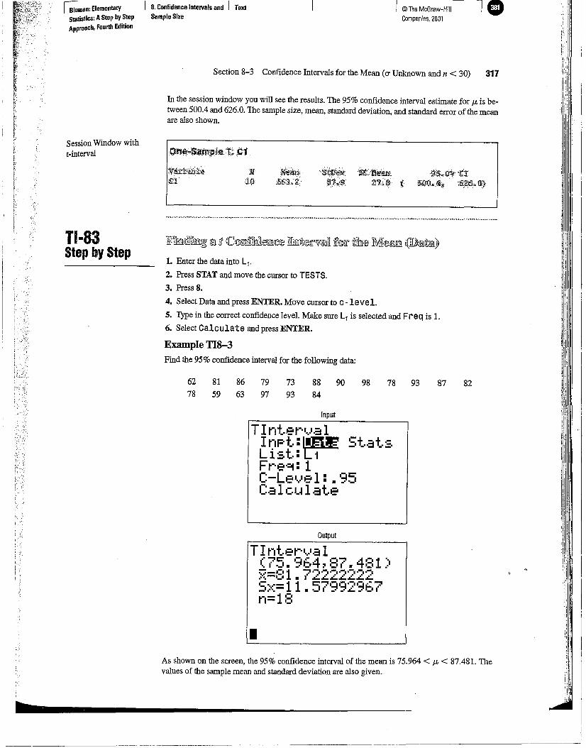
8287
95"[i~1tI
'iWlr,,,,Al~, 1~,i$,,':l1i~
93
© The McGraw-HiliCompanies. 2001
789890
Input
.:ai~[)J0.~, ~:;'J!ie;Wfi;
~.'7;,,;~(~1:.,a: t
88
84
73
93
J~tii!u:i::5&;3.2:'
79
97
Output
TI nt.er'1...1a 1... 71:' g':::4 C,,,,,:, 4P1 .~'.1·_1 •• ,_, ';IV(. _'.':- .-. 1 ..., .-. .-..-..-..-..-..-..:-::=I:' .... L. L L. L'::' L L.- 11 5-' - .- .-. - ...'- ....- .' q '.... t-: ..._' .•..• - • I.· ..:.;. .' _' 1
n=18
TInter'...'alInpt:lm,E St.at.sList.:~Fr·e·=:.j: 1(:-Le'..,1e 1: • 95Calculate
•
86
63
81
59
62
78
:'\re:lJjj;.~,'i~Jl:J' , ,
In the session window you will see the results. The 95% confidence interval estimate for p: is between 500.4 and 626.0. The sample size, mean, standard deviation, and standard error of the meanare also shown.
Section 8-3 Confidence Intervals for the Mean (0"Unknown and n < 30) 317
1. Enter the data into L1•
2. Press STAT and move the cursor to TESTS.
3. Press 8.
4. Select Data and press ENTER. Move cursor to c-level.5. Type in the correct confidence level. Make sure L1 is selected and Freq is 1.
6. Select Calculate and press ENTER.
Example TI8-3Find the 95% confidence interval for the following data:
As shown on the screen, the 95% confidence interval of the mean is 75.964 < t-t < 87.481. Thevalues of the sample mean and standard deviation are also given.
B. Confidence IntelVals and I TextSample Size
SessionWindow witht-interval
TI·83Step by Step
r;;:man: ElementaryStatistics: AStepbyStepApproach, Fourth Edition
h _

G Blumen: ElemelllaryStatistics: A Step byStepApproach, Fourth Edition
B. Confidence IlIIervalsand TextSemple Size
© The McGraw-HiliCompanies. 2001
318 Chapter 8 Confidence Intervals and Sample Size
As shown, the 95% confidence interval is 0.26277 < JL < 0.37723.
Output
TI t'",+..er'-.Ja 1(.26277:0.37723)5<=.32S>~=. 08,.-,=10
Input
Tlnter'....alI,.-,p+..:Da+..a~:;::. -:::?r-. •• ........Sx:.08,.-,: 10C-Level:.95Calculate
fifum!LUH:[d~&111 OGmllifHi!l(!3IT~{('''if; mreil'¥7il~ [@rI' ftllitl1:e M®wJ(!l (~f£~twJ)
1. Press STAT and move the cursor to TESTS.
2. Press 8 for TInterval.
3. Select Stats and press ENTER. Move cursor to x.4. Enter the value for the sample mean, X.5. Enter the value for the sample standard deviation, SX'
6. Enter the sample size, n.
7. Type in the correct confidence interval.
8. Select Calculate and press ENTER.
Example TI8-4As in Example 8-6, find the 95% confidence interval when X = 0.32, s = 0.08, and n = 10.
A USA Today Snapshots feature (July 2, 1993) stated that 12% of the pleasure boats inthe United States were named Serenity. The parameter 12% is called a proportion. Itmeans that of all the pleasure boats in the United States, 12 out of every 100 are namedSerenity. A proportion represents a part of a whole. It can be expressed as a fraction, decimal, or percentage. In this case, 12% = 0.12 = l~ orrs. Proportions can also representprobabilities. In this case, if a pleasure boat is selected at random, the probability that itis called Serenity is 0.12.
Proportions can be obtained from samples or populations. The following symbolswill be used.
"
-Confidence Intervalsand Sample Size forProportionsI',Ibjactlve 4. Rnd theconfidence interval foraproportion.
i!FL ·-· ...--.....
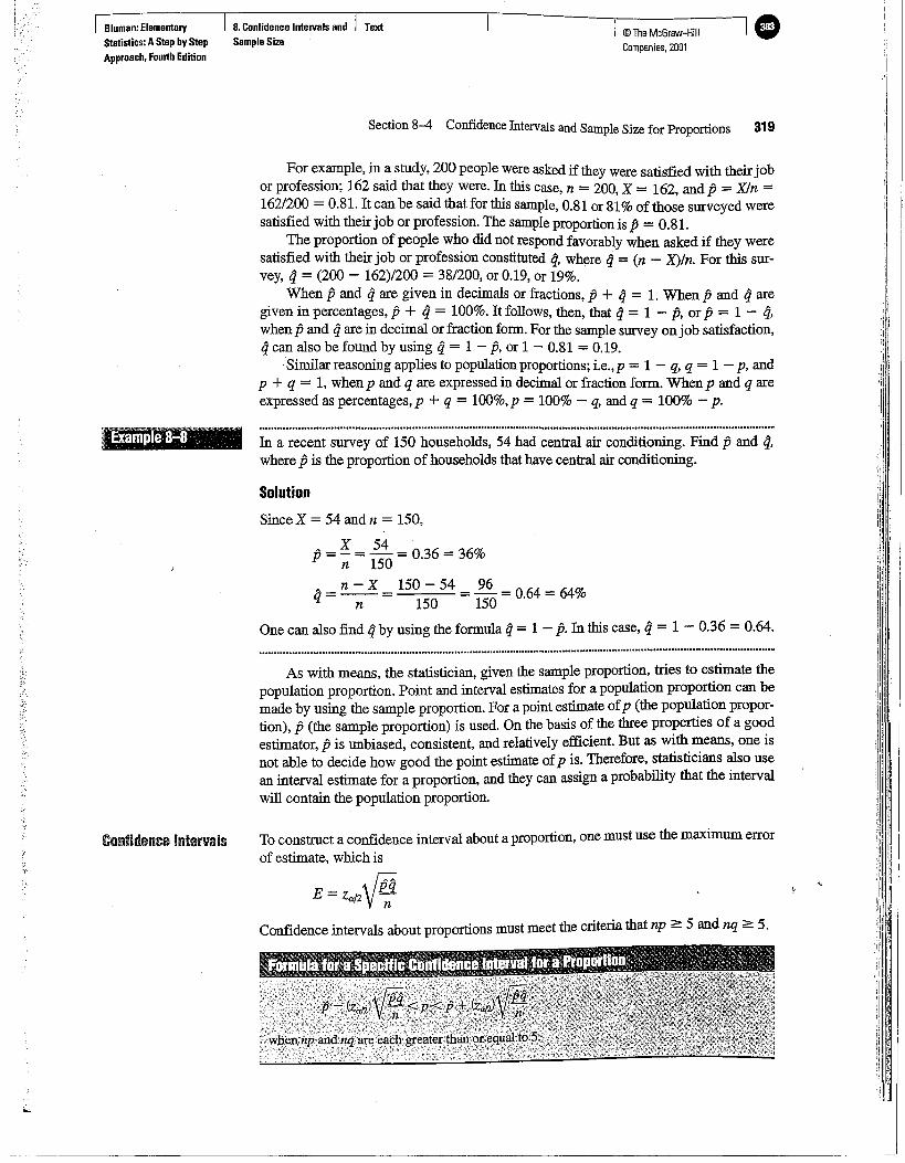
8luman: ElementaryStatistics: AStep byStepApproach, Fourth Edition
8.Confidence Intervalsand TextSample Size
© The McGraw-HiliCompanies, 2001
, ampeH
Confidence Intervals
Section 8-4 Confidence Intervals and Sample Size for Proportions 319
For example, in a study, 200 people were asked if they were satisfied with their jobor profession; 162 said that they were. In this case, n = 200, X = 162, and p = Xln =162/200 = 0.81. It can be said that for this sample, 0.81 or 81% of those surveyed weresatisfied with their job or profession. The sample proportion is p = 0.81.
The proportion of people who did not respond favorably when asked if they weresatisfied with their job or profession constituted q, where q= (n - X)ln. For this survey, q= (200 - 162)/200 = 38/200, or 0.19, or 19%.
When p and q are given in decimals or fractions, p + q = 1. When p and q aregiven in percentages, p + ij = 100%. It follows, then, that q = 1 - p, or p = 1 - q,whenp and ij are in decimal or fraction form. For the sample survey on job satisfaction,ij can also be found by using q= 1 - p, or 1 - 0.81 = 0.19.
-Similar reasoning applies to population proportions; i.e.,p = 1 - q, q = 1 - p, andp + q = 1, when p and q are expressed in decimal or fraction form. When p and q areexpressed as percentages, p + q = 100%, p = 100% - q, and q = 100% - p.
In a recent survey of 150 households, 54 had central air conditioning. Find p and ij,where p is the proportion of households that have central air conditioning.
Solution
Since X = 54 and n = 150,
P= ~ = :5~ = 0.36 = 36%
q= n - X = 150 - 54 =~ = 064 = 64%n 150 150 .
One can also find qby using the formula q= 1 - p. In this case, q = 1 - 0.36 = 0.64...............................................................................................................................................................................
As with means, the statistician, given the sample proportion, tries to estimate thepopulation proportion. Point and interval estimates for a population proportion can bemade by using the sample proportion. For a point estimate of p (the population proportion), p (the sample proportion) is used. On the basis of the three properties of a goodestimator, p is unbiased, consistent, and relatively efficient. But as with means, one isnot able to decide how good the point estimate ofp is. Therefore, statisticians also usean interval estimate for a proportion, and they can assign a probability that the interval
will contain the population proportion.
To construct a confidence interval about a proportion, one must use the maximum error
of estimate, which is
E = Za/zVi!-Confidence intervals about proportions must meet the criteria that np 2:: 5 and nq 2:: 5.
Rounding Rule for a Confidence Interval for a Proportion Round off to three decimalplaces.
CD Bluman:Elamentary 8.Confidence Intervalsand Text
Statistics: A Step.byStep SampleSize
Approach.FourthEdition
320 Chapter 8 Confidence Intervals and Sample Size
© The McGraw-HiliCompanies. 2001
'.'i
(0.12)(0.88)
500
ample
" Example 8-10
Sample Size forProportions
A sample of 500 nursing applications included 60 from men. Find the 90% confidenceinterval of the true proportion of men who applied to the nursing program.
Solution
Since a = 1 - 0.90 = 0.10, and Za/2 = 1.65, substituting in the formula
p - (Za/2)Vi!- < p < P+ (Za/2)Vi!-whenft = 601500 = 0.12 and q= 1 - 0.12 = 0.88, one gets
0.12 - (1.65) (O.1~~~.88) < p < 0.12 + (1.65)
0.12 - 0.024 < P < 0.12 + 0.024
0.096 < P < 0.144
or 9.6% < P < 14.4%
Hence, one can be 90% confident that the percentage of men who applied is between9.6% and 14.4%.
When a specific percentage is given, the percentage becomes p when it is changedto a decimal. For example, if the problem states that 12% of the applicants were men,then p = 0.12.
A survey of 200,000 boat owners found that 12% of the pleasure boats were namedSerenity. Find the 95% confidence interval of the true proportion of boats named Serenity. (Source: USA Today Snapshot, July 2, 1993)
Solution
From the Snapshot, ft = 0.12 (i.e., 12%), and n = 200,000. Since Za/2 = 1.96, substituting in the formula
ft - (Za/2)Vi!- < p < p + (Za/2)Vi!- yields
0.12 - (1.96) (02~,~~8) < p < 0.12 + (1.96) (02~,~~8)
0.119 < P < 0.121
Hence, one can say with 95% confidence that the true percentage of boats named Serenity is between 11.9% and 12.1%.
In order to find the sample size needed to determine a confidence interval about a proportion, use the following formula.
.:::.;C;'i
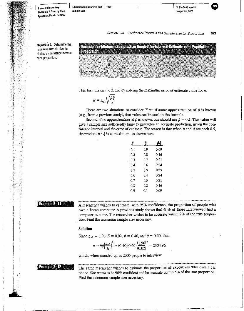
.............................................................................................................................................................................
which, when rounded up, is 2305 people to interview.
© The McGraw-HiliCompanies. 2001
fiq0.09
0.16
0.21
0.24
0.25
0.24
0.21
0.16
0.09
0.9
0.8
0.7
0.6
0.50.4
0.3
0.2
0.1
0.1
0.2
0.3
0.4
0.50.6
0.70.8
0.9
A researcher wishes to estimate, with 95% confidence, the proportion of people whoown a home computer. A previous study shows that 40% of those interviewed had acomputer at home. The researcher wishes to be accurate within 2% of the true proportion. Find the minimum sample size necessary.
There are two situations to consider. First, if some approximation of P is known(e.g., from a previous study), that value can be used in the formula.
Second, ifno approximation of Pis mown, one should use P= 0.5. This value willgive a sample size sufficiently large to guarantee an accurate prediction.'given the confidence interval and the error of estimate. The reason is that when Pand qare each 0.5,the product P. qis at maximum, as shown here.
Section 8-4 Confidence Intervals and Sample Size for Proportions 321
This formula can be found by solving the maximum error of estimate value for n:
E = Za/2Vi!-
Solution
Since Za/2 = 1.96, E = 0.02, P= 0040, and q= 0.60, then
n =pq(~r = (OAO)(0.60)(~:~~r = 2304.96
8.Confidence Intervalsand TextSample Size
Example 8+11
Bluman: ElementaryStatistics: AStep byStepApproach, Fourth Edition
ObjectiveS. Determine theminimum sample size forfinding aconfidence intervalforaproportion.
..............................................................................................................................................................................The same researcher wishes to estimate the proportion of executives who own a carphone. She wants to be 90% confident and be accurate within 5% of the true proportion.Find the minimum sample size necessary.

Blumen: ElementeryStatistics:AStep byStepApproech, Fourth Edition
I 8.Confidence Intervalsand I TextSempleSize
© The McGraw-HiliCompanies, 2001
In determining the sample size, the size of the population is irrelevant. Only the degree of confidence and the maximum error are necessary to make the determination.
Solution
Since no prior knowledge of p is known, statisticians assign the values p = 0.5 andfj =0.5. The sample size obtained by using these values will be large enough to ensurethe specified degree of confidence. Hence,
n = pq(~r = (O.5)(O.5)(~:~~r = 272.25
which, when rounded up, is 273 executives to ask.
8-57. A survey of 90 families showed that 40 owned atleast one gun. Find the 95% confidence interval of the trueproportion of families who own at least one gun.
8-58. In a certain state, a survey of 500 workers showedthat 45% belonged to a union. Find the 90% confidenceinterval of the true proportion of workers who belong to aunion.
8-59. For a certain age group, a study of 100 people whodied showed that 25% had died of cancer. Find the
8-53. A survey found that out of 200 workers, 168 saidthey were interrupted three or more times an hour by phonemessages, faxes, etc. Find the 90% confidence interval ofthe population proportion of workers who are interruptedthree or more times an hour.
Source:Basedon informationfrom USAToday Snapshot, August6,1997.
8-54. A survey of 120 female freshmen showed that 18 didnot wish to work after marriage. Find the 95% confidenceinterval of the true proportion of females who do not wishto work after marriage.
8-55. A study by the University of Michigan found thatone in five 13- and l4-year-olds is a sometime smoker. Tosee how the smokingrate of the students at a large schooldistrict compared to the national rate, the superintendentsurveyed 200 13- and l4-year-old students and found that23% said they were sometime smokers. Find the 99%confidence interval of the true proportion and compare thiswith the University of Michigan's study.
Source:USAToday, July 20, 1995.
8-56. A survey of 80 recent fatal traffic accidents showedthat 46 were alcohol-related. Find the 95% confidenceinterval of the true proportion of fatal alcohol-relatedaccidents.
322 Chapter 8 ConfidenceIntervals and Sample Size
8-47. In each case, findp and q.a. n = 80 andX= 40b. n = 200 andX = 90c. n = 130 and X = 60d. n =60 and X= 35e. n = 95 and X= 43
8-48. (aus) Findp and qfor each percentage. (Use eachpercentage forp.)a. 12%b.29%c. 65%d.53%e. 67%
8-49. A U.S. TravelData Center surveyconductedforBetterHomesandGardens of 1500adultsfound that 39%said that they wouldtake more vacations this year than lastyear.Find the 95% confidenceintervalof the true proportionof adults who said that they will travelmore this year.
Source:USAToday, April20, 1995.
8-50. Arecent study of loa people in Miami found 27 wereobese.Find the 90% confidenceintervalof the populationproportionof individualsliving in Miamiwho are obese.
Source: Based on information from the Centerfor DiseaseControlandPrevention, USAToday, March4, 1997.
8-51. An employment counselor found that in a sample of100 unemployed workers, 65% were not interested inreturning to work. Find the 95% confidenceinterval of thetrue proportion of workers who do not wish to return towork.
8-52. A Today/CNN/GallupPoll of 1015 adults found that13% approved of the job Congress was doingin 1995. Findthe 95% confidence interval of the true proportion of adultswho feel this way.
Source: USAToday, March31, 1995.
.'

proportion of individuals who die of cancer in that agegroup. Use the 98% confidence interval.
8-60. A researcher wishes to be 95% confident that her~stimateof the true proportion of individuals who traveloverseas is within,0.04 of the true proportion. Find thesample size necessary. In a prior study, a sample of 200people showed that 80 traveled overseas last year.
8-61. A medical researcher wishes to determine thepercentage of females who take vitamins. He wishes to be99% confident that the estimate is within 2 percentagepoints of the true proportion. A recent study of 180 femalesshowed that 25% took vitamins.a. How large should the sample size be?b. If no estimate of the sample proportion is available,
how large should the sample be?
8-62. A recent study indicated that 29% of the 100 womenover 55 in the study were widows.a. How large a sample must one take to be 90% confident
that the estimate is within 0.05 of the true proportion ofwomen over 55 who are widows?b. If no estimate of the sample proportion is available,
how large should the sample be?
8-63. A researcher wishes to estimate the proportion ofadult males who are under 5 feet 5 inches tall. She wants to
Companies. 2001
be 90% confident that her estimate is within 5% of the trueproportion.
a. How large a sample should be taken if in a sample of300 males, 30 were under 5 feet 5 inches tall?b. If no estimate of the sample proportion is available,
how large should the sample be?
8-64. An educator desires to estimate, within 0.03, the trueproportion of high school students who study at least 1 houreach school night. He wants to be 98% confident.a. How large a sample is necessary? Previously, he
conducted a study and found that 60% of the 250 studentssurveyed spent at least 1 hour each school night studying.b. If no estimate of the sample proportion is available,
how large should the sample be?
*8-65. If a sample of 600 people is chosen and theresearcher desires to have a maximum error of estimate of4% on the specific proportion who favor gun control, findthe degree of confidence. A recent study showed that 50%were in favor of some form of gun control.
*8-66. In a study, 68% of 1015 adults said they believe theRepublicans favor the rich. If the margin of error was 3percentage points, what was the confidence interval usedfor the proportion?
Source: USAToday, March 31, 1995.
Section 8-4 Confidence Intervals and Sample Size for Proportions 323
cr.l? ""I"' /P it:!l,J1 11' ":ill '" TIl) ....Jt'"M.1 ,nnl\(lillJr1~ ;ID fl..'/(D'!Elill!©i2JITll(C',J; ilmUvBlr'W'i£\ill tFIDIf' Iffi Ji ifif.k1J!.D@lPJ]@1ill
MINITAB will calculate a confidence interval given the statistics from a sample or given the rawdata. These instructions use the sample information in Example 8-9.
Example MT8-3There were 500 nursing applications in a sample, including 60 from men. Find the 90% confidence interval of the actual proportion of male applicants.
1. Select Stat>Basic Statistics>1 Proportion.
SampleSize
I Proportion Dialog Box
MINITABStep by Step
I UIUIIIO -._-~- •
Statistics;A Step byStepApproach, Fourth Edition
2. Click on the button for Summarized data.

I © The McGraw-HiliCompanies. 2001
I-PropZInt(.09152~.14848). 1~~.=. L.n=500
::;N':
'j,~'.:!~
I-ProF'Z Int>::: 60
·c--0n ....II:::!C-Level: .95CaLcu l at.e
3. Click in the box for Number of trials and enter 500.
4. In the Number of successes box enter 60.
5. Click on [Options].
I 8.Confidence Intervels end , TextSample Size
The 95% confidence level for pis 0.09152 < P < 0.14848.Pis also given.
1. Press STAT and move the cursor to TESTS.
2. Press A (ALPHA, MATH) for 1 - PropZlnt.3. Enter the value for X.
4. Enter the value for n.
5. Type in the correct confidence interval.
6. Select Calculate and press ENTER.
Example TI8-5Find the 95% confidence interval of p when X = 60 and n = 500, as in Example 8-9.
Input Output
The results for the confidence interval will be displayed in the session window. The populationproportion is most likely between 10% and 14%. The Z- and P-values shown are used in hypothesis testing, covered in the next chapter.
6. Type 90.0 for the confidence level.
7. Check the box for Use test and interval based on normaldist ribution.
8. Click [OK] twice.
1 Proportion OptionsDialog Box
324 Chapter 8 Confidence Intervals and Sample Size
;.
Confidence Interval for1 Proportion
TI·83Step by Step
CD I Bluman: ElementllryStatistics: AStepbyStepApproach. Fourth Edition

d.t. =1
Section 8-5 Confidence Intervals for Variances and Standard Deviations 325
© The McGraw-HiliCompanies. 2001
In order to calculate these confidence intervals, a new statistical distribution isneeded. It is called the chi-square distribution.
The chi-square variable is similar to the t variable in that its distribution is a familyof curves based on the number of degrees of freedom. The symbol for chi-square is X2
(Greek letter chi, pronounced "ki"). Several of the distributions are shown in Figure8-9, along with the corresponding degrees of freedom. The chi-square distribution is obtained from the values of (n - 1)s2/cr when random samples are selected from a normally distributed population whose variance is cr.
In the previous section, confidence intervals were calculated for means and proportions.This section will explain how to find confidence intervals for variances and standard deviations. In statistics, the variance and standard deviation of a variable are as importantas the mean. For example, when products that fit together (such as pipes) are manufactured, it is important to keep the variations of the diameters of the products as small aspossible; otherwise, they will not fit together properly and have to be scrapped. In themanufacture of medicines, the variance and standard deviation of the medication in thepills play an important role in making sure patients receive the proper dosage. For thesereasons, confidence intervals for variances and standard deviations are necessary.
B. Confidence Intervals and TextSample Size
Confidence Intervalsfor Variances andStandard DeviationsObjective 6. Find aconfidence interval foravariance and astandarddeviation.
Bluman: ElementaryStatistics: AStep byStepApproach. Fourth Edition
The Chi-SquareFamily of Curves
Figure 8-9

•
e 8luman: ElementaryStatistics:AStepbyStepApproach. Fourth Edition
8.Confidence Intervals and TextSample Size
© The McGraw-HiliCompanies, 2001
326 Chapter 8 Confidence Intervals and Sample Size
A em-square variable cannot be negative, and the distributions are positivelyskewed. At about 100 degrees of freedom, the em-square distribution becomes somewhat symmetrical. The area under each chi-square distribution is equal to 1.00 or 100%.
Table G in Appendix C gives the values for the chi-square distribution. These values are used in the denominators of the formulas for confidence intervals. Two differentvalues are used in the formula. One value is found on the left side of the table and theother is on the right. For example, to find the table values corresponding to the 95% confidence interval, one must first change 95% to a decimal and subtract it from 1 (1 - 0.95= 0.05). Then divide the answer by 2 (cd2 = 0.05/2 = 0.025). This is the column on theright side of the table, used to get the values for :dght. To get the value for Xfeft, subtractthe value of cd2 from 1 (1 - 0.0512 = 0.975). Finally, find the appropriate row corresponding to the degrees of freedom, n - 1. A similar procedure is used to find the val-.ues for a 90% or 99% confidence interval.
1'. .: ',"'.,' :.' ",,','. ' .: ,".::
,Jhex~distrlbutioiJwith'2n.
,dellrees,fq~mulated", , i{"inathemalician'.name
,;H,¥"s,hel·jD;1.~f)~~6.il~',·\.was'studYitJ~1h~;:ac;cu •
!~:;~aM~, ' ';contdh
i>111~flt
. Example 8-'13
Figure 8-10x2Table forExample 8-13
Find the values for ~ght and Xfeft for a 90% confidence interval when n = 25.
Solution
To find X~ght, subtract 1 - 0.90 = 0.10 and divide by 2 to get 0.05.To find Xfeft' subtract 1 - 0.05 to get 0.95. Hence, use the 0.95 and 0.05 columns
and the row corresponding to 24 d.f. See Figure 8-10.
The answers are
X~ght = 36.415
X~ft = 13.848
The best estimates for if and (T are i2and s respectively.In order to find confidence intervals for variances and standard deviations, one
must assume that the variable is normally distributed.The formulas for the confidence intervals are shown next.
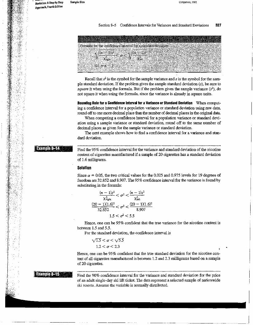
Companies. 2001
Section 8-5 Confidence Intervals for Variances and Standard Deviations 327
Recall that i2 is the symbol for the sample variance and s is the symbol for the sample standard deviation. If the problem gives the sample standard deviation (s), be sure tosquare it when using the formula. But if the problem gives the sample variance (S2), donot square it when using the formula, since the variance is already in square units.
Rounding Rule for a Confidence Interval for a Variance or Standard Deviation When computing a confidence interval for a population variance or standard deviation using raw data,round off to one more decimal place than the number of decimal places in the original data.
When computing a confidence interval for a population variance or standard deviation using a sample variance or standard deviation, round off to the same number ofdecimal places as given for the sample variance or standard deviation.
The next example shows how to find a confidence interval for a variance and standard deviation.
Find the 90% confidence interval for the variance and standard deviation for the priceof an adult single-day ski lift ticket. The data represent a selected sample of nationwideski resorts. Assume the variable is normally distributed.
Find the 95% confidence interval for the variance and standard deviation of the nicotinecontent of cigarettes manufactured if a sample of 20 cigarettes has a standard deviationof 1.6 milligrams.
Solution
Since a = 0.05, the two critical values for the 0.025 and 0.975 levels for 19 degrees offreedom are 32.852 and 8.907. The 95% confidence interval for the variance is found bysubstituting in the formula:
(n - 1)s2 2 (n - 1)i22 <0'< 2
X right Xleft
(20 - 1)(1.6)2 2 (20 - 1)(1.6)232.852 < 0' < 8.907
1.5 < cr < 5.5
Hence, one can be 95% confident that the true variance for the nicotine content isbetween 1.5 and 5.5.
For the standard deviation, the confidence interval is
yff.5 < 0' < V531.2 < 0' < 2.3
t
Hence, one can be 95% confident that the true standard deviation for the nicotine content of all cigarettes manufactured is between 1.2 and 2.3 milligrams based on a sampleof 20 cigarettes.
Sample Size
-
I ---
StBtistics: AStepbyStepApproach. Fourth Edition
e Bluman: ElementaryStatistics: AStep byStepApproach. Fourth Edition
8.Confidence Intervalsand TextSample Size
© The McGraw-HiliCompanies. 2001
328 Chapter 8 Confidence Intervals and Sample Size
$59
39
$54
49
$53
46$52
49
$51
48
Source: USA Today, October 6, 1998.
For the standard deviation
8-71. Find the 90% confidence interval for the varianceand standard deviation for the time it takes an inspector tocheck a bus for safety if a sample of 27 buses has astandard deviation of 6.8minutes. Assumethe variable isnormally distributed.
8-72. Find the 99% confidence interval for the varianceand standard deviation of the weights of 25 galloncontainers of motor oil if a sample of 14 containers has avariance of 3.2. The weights are given in ounces. Assumethe variable is normally distributed.
8-73. The sugar content (in grams) for a random sample of4-ounce containers of applesauce is shown. Find the 99%confidence interval for the population variance andstandard deviation. Assume the variable is normallydistributed.
y'I5 < 0" < V76.3
3.87 < 0" < 8.73
Note: If you are using the standard deviation instead (as in Example 8-14) of thevariance, be sure to square the standard deviation when substituting in the formula.
Hence one can be 90% confident that the standard deviation for the price of all singleday ski lift tickets of the population is between $3.87 and $8.73 based on a sampleof 10 nationwide ski resorts. (Two decimal places are used since the data are in dollarsand cents.)
Solution
STEP 1 Find the variance for the data. Use the formulas in Chapter 3 or yourcalculator.The variance s'l = 28.2
STEP 2 Find X~ght and Xfeft from Table G in Appendix C. Since a = 0.10, the twocritical values are 3.325 and 16.919 using d.f. = 9 and 0.95 and 0.05.
STEP 3 Substitute in the formula and solve.
(n - 1)s2 2 (n - 1)s'l2 <0"< 2
X right X left
(10 - 1)(28.2) 2 (10 - 1)(28.2)16.919 < 0" < 3.325·
15.0 < 0"2 < 76.3
8-67. What distribution must be used when computingconfidence intervals for variances and standard deviations?
8:-68. What assumption must be made when computingconfidence intervals for variances and standard deviations?
8-69. Using Table G, find the values for Xreft and Xaght.a. a = 0.05 n = 16b. a = 0.10 n = 5c. a = 0.01 n = 23d. a = 0.05 n = 29e. a = 0.10 n = 14
8-70. Find the 95% confidence interval for the varianceand standard deviation for the lifetime of batteries if asample of 20 batteries has a standard deviation of 1.7months. Assume the variable is normally distributed.
I.,J
,:tj
------------------- ;.

An important aspect of inferential statistics is estimation. Estimations of parameters ofpopulations are accomplished by selecting a random sample from that population andchoosing and computing a statistic that is the best estimator of the parameter. A good estimator must be unbiased, consistent, and relatively efficient. The best estimators of J.L andp are X and p, respectively. The best estimators of a2and (J' are S2 and s, respectively.
There are two types of estimates of a parameter: point estimates and interval estimates. A point estimate is a specific value. For example, if a researcher wishes to estimate the average length of a certain adult fish, a sample of the fish is selected andmeasured. The mean of this sample is computed-e.g., 3.2 centimeters. From this sample mean, the researcher estimates the population mean to be 3.2 centimeters.
The problem with point estimates is that the accuracy of the estimate cannot be determined. For this reason, statisticians prefer to use the interval estimate. By computingan interval about the sample value, statisticians can be 95% or 99% (or some other percentage) confident that their estimate contains the true parameter. The confidence levelis determined by the researcher. The higher the confidence level, the wider the intervalof the estimate must be. For example, a 95% confidence interval of the true mean lengthof a certain species of fish might be
3.17 < J.L < 3.23
whereas the 99% confidence interval might be
3.15 < J.L < 3.25
When the confidence interval of the mean is computed, the z or t values are used,depending on whether or not the population standard deviation is known and depending
Summary
Source: Pittsburgh Tribune Review, July 6,1997.
12.03, 12.10,12.02, 11.98, 12.00, 12.05, 11.97, 11.99.
© The McGraw-HiliCompanies, 2001
Section 8-6 Summary 329
8-77. A servicestation advertises that customers will haveto wait no more than 30 minutes for an oil change. Asample of 28 oil changes has a standard deviation of5.2 minutes.Find the 95% confidence interval of thepopulation standard deviation of the time spent waitingfor an oil change.
8-78. Find the 95% confidence interval for the varianceand standarddeviation of the ounces of coffee that amachine dispensesin 12-ouncecups. Assume the variableis normallydistributed.The data are given here.
*8-79. A confidenceinterval for a standard deviation forlarge samplestaken from a normally distributed populationcan be approximatedby
s ss - za/2 • V2ii < (T < S + za/2 • V2ii
Find the 95%confidenceinterval for the populationstandard deviationof calculator batteries. A sample of200 calculatorbatteries has a standard deviation of18 months.
I 8.Confidence Intervals and I TextSample Size
18.6 19.5 20.2 20.4 19.3
21.0 20.3 19.6 20.7 18.9
22.1 19.7 20.8 18.9 20.7
21.6 19.5 20.1 20.3 19.9
$26.69 $13.88 $28.37 $12.00
75.37 7.50 47.50 43.00
3.81 53.81 13.62 45.12
6.94 28.25 28.00 60.50
40.25 10.87 46.12 14.75
IlIURlan: Elementary'surtisliCS:AStepbyStep,APproach. Fourth Edition
-.. - ,,
8-74. Find the 90% confidenceinterval for the varianceandstandarddeviation of the ages of seniors at Oak ParkCollege if a sample of 24 students has a standard deviation
, of 2.3 years.Assume the variable is normally distributed.
8-75. Find the 98% confidenceinterval for the varianceandstandarddeviation for the time it takes a telephonecompany to transfer a call to the correct office. A sample of15callshas a standard deviation of 1.6 minutes. Assumethe variableis normally distributed.
8-76. A random sample of stock prices per share is shown.Find the 90% confidence interval for the variance andstandard deviation for the prices. Assume the variable isnormallydistributed.
L _
e Bluman: ElementaryStatistics: A Step byStepApproach, Fourth Edition
8.Confidence IntelVals and TextSample Size
© The McGraw-HiliCompanies, 2001
330 Chapter 8 Confidence Intervals and Sample Size
relatively efficientestimator 299
t distribution 311
unbiased estimator 299
maximum error ofestimate 301
point estimate 299
proportion 318
Formula for the confidence interval for a variance:
(n - 1)82 (n - 1)82"'---=-"'-- < u 2 < "'---::-"'--
.i:lghl MortFormula for confidence interval for a standard deviation:y(n -1)82 y(n -1)82
<u<rrighl Meft
Formula for the sample size for proportions:
n=pq(~r
deviation of the sample was 6.2 hours. Find the 90%confidence interval of the true mean. How does thiscompare with the TV Guide findings?
Source:TV Guide 43, no. 30 (1995), p. 26.
degrees of freedom 312
estimation 298
estimator 299
interval estimate 299
on the size of the sample. If a is known or n ;::: 30, the z values can be used. If o:is notknown, the t values must be used when the sample size is less than 30, and the population is normally distributed.
Closely related to computing confidence intervals is determining the sample size tomake an estimate of the mean. The following information is needed to determine theminimum sample size necessary.
1. The degree of confidence must be stated.
2. The population standard deviation must be known or be able to be estimated.
3. The maximum error of estimate must be stated.
Confidence intervals and sample sizes can also be computed for proportions, usingthe normal distribution, and confidence intervals for variances and standard deviationscan be computed using the chi-square distribution.
chi-squaredistribution 325
confidence interval 300
confidence level 300
consistent estimator 299
8-80. TV Guide reported that Americans have theirtelevision sets turned on an average of 54 hours per week.A researcher surveyed 50 local households and found theyhad their sets on an average of 47.3 hours. The standard
Formula for the confidence interval of the mean when a isknown (when n 2:: 30, S can be used if o is unknown):
x-(Z0{2}:n) < JL < X +f0{2}:n)Formula for the sample size for means:
n = (ZW~ urwhere E is the maximum error.
Formula for the confidence interval of the mean when a isunknown and n < 30:
X - ta/2(v,,) < JL < X + ta/2(v,,)Formula for the confidence interval for a proportion:
ft - (z0{2)Vi! < P < ft + (z0{2)Vi!whereft = X/n and q= 1 - ft.
©The McGraw-HiliCompanies. 2001
interval of the true proportion of all adults who favorvisiting historical sites as vacations.
Source: USA Today, April 20, 1995.
8-89. In a study of 200 accidents that required treatment inan emergency room, 40% occurred at home. Find the 90%confidence interval of the true proportion of accidents thatoccur at home.
Section 8--6 Summary 331
8-90. In a recent study of 100 people, 85 said that theywere dissatisfied with their local elected officials. Find the90% confidence interval of the true proportion ofindividuals who are dissatisfied with their local electedofficials.
8-91. A nutritionist wishes to determine, within 2%, thetrue proportion of adults who snack before bedtime. If shewishes to be 95% confident that her estimate contains thepopulation proportion. how large a sample will she need? Aprevious study found that 18% of the 100 people surveyedsaid they did snack before bedtime.
8-92. A survey of 200 adults showed that 15% playedbasketball for regular exercise. If a researcher desires tofind the 99% confidence interval of the true proportion ofadults who play basketball and be within 1% of the truepopulation, how large a sample should be selected?
8-93. The standard deviation of the diameter of 28 orangeswas 0.34 inch. Find the 99% confidence interval of the truestandard deviation of the diameters of the oranges.
8-94. A random sample of 22 lawn mowers was selected.and the motors were tested to see how many miles pergallon of gasoline each one obtained. The variance of themeasurements was 2.6. Find the 95% confidence interval ofthe true variance.
8-95. A random sample of 15 snowmobiles was selected,and the lifetimes (in months) of the batteries was measured.The variance of the sample was 8.6. Find the 90%confidence interval of the true variance.
8-96. The heights of 28 police officers from a large-citypolice force were measured. The standard deviatio~ of thesample was 1.83 inches. Find the 95% confidence mtervalof the standard deviation of the heights of the officers.
8.Confidence Intervals and TextSample Size
Bluman:ElementaryStatistics: A StepbyStepApproach. Fourth Edition
l Would You Change the Channel? Revisited!The estimates given in the article are point estimates. However, sin~e the mar~n of er\ ror is stated to be 3 percentage points, an interval estimate can easily be.obtamed. For1 example. if 45% of the people changed the channel, then the confidence interval of ~e1 true percentages of people who changed channels would be 42% < P < 48%. The arti1 cle fails to state whether a 90%, 95%. or some other percentage was used for the confi1dence interval.
8-81. A study of 36 members of the Central Park Walkersshowed that they could walk at an average rate of 2.6 milesper hour. The sample standard deviation is 0.4. Find the95% confidence interval for the mean for all walkers.
8-82. The average weight of 60 randomly selectedcompact automobiles was 2627 pounds. The samplestandard deviation was 400 pounds. Find the 99%confidence interval of a true mean weight of theautomobiles.
8-83. A U.S. Travel Data Center survey reported thatAmericans stayed an average of 7.5 nights when they wenton vacation. The sample size was 1500. Find the 95%confidence interval of the true mean. Assume the standarddeviation was 0.8 day.
Source: USA Today, April20, 1995.
8-84. A recent study of 25 commuters showed that theyspent an average of $18.23 on public transportation perweek. The standard deviation of the sample was $3.00.Find the 95% confidence interval of the true mean. Assumethe variable is normally distributed.
8-85. For a certain urban area, in a sample of five months,an average of 28 mail carriers were bitten by dogs eachmonth. The standard deviation of the sample was 3. Findthe 90% confidence interval of the true mean number ofmail carriers who are bitten by dogs each month. Assumethe variable is normally distributed.
8-86. A researcher is interested in estimating the averagesalary of teachers in a large urban school district. She wantsto be 95% confident that her estimate is correct. If thestandard deviation is $1050, how large a sample is neededto be accurate within $200?
8-87. A researcher wishes to estimate, within $25, the trueaverage amount of postage a community college spendseach year. If she wishes to be 90% confident, how large asample is necessary? The standard deviation is known tobe $80.
8-88. A U.S. Travel Data Center's survey of 1500 adultsfound that 42% of respondents stated that they favorhistorical sites as vacations. Find the 95% confidence
------r-----r-------'T---~--Ie

e 8luman: ElementaryStatistics:AStepbyStepApproach. Fourth Edition
8.Confidence Intervals and TextSample Size
© The McGraw-HiliCompanies, 2001
332 Chapter 8 Confidence Intervals and Sample Size
Using the formula given in Section 8-4, a minimum sample size of 1068 would beneeded to obtain a 95% confidence interval for p, as shown next. Use p and qas 0.5,since no value is known for p.
n =pq(~r
(1.96)2
n = (0.5)(0.5) 0.03 = 1067.1
n = 1068
intervals of the mean length in miles of major NorthAmerican rivers. Find the mean of all the values anddetermine if the confidenceintervals contain the mean.
S. From Data Set VI in Appendix D, select a sample of 20values and find the 90% confidence interval of the meanof the number of acres.Find the mean of all the valuesand determineif the confidence interval contains themean.
---~~ - _._._._._----_.__.~-_ ..----------
6. From Data Set XIV in Appendix D, select a sample of20 weightsfor the Pittsburgh Steelers and find theproportion of players who weigh over 250 pounds.Construct a 95% confidenceinterval for this proportion.Find the proportionof all Steelers who weigh more than250 pounds. Does the confidence interval contain thisvalue?
b. Largerc. The samed. It cannotbe determined
6. The best point estimate of the population mean isa. The samplemeanb. The samplemedianc. The samplemoded. The samplemidrange
7. When the populationstandard deviation is unknownand sample sizeis less than 30, what table value shouldbe used in computinga confidence interval for a mean?a.zb. tc. chi-squared. None of the above
Complete the following statements with the best answer.
8. A good estimator shouldbe , and
The Data Bank is found in Appendix D, or on the WorldWide Web by following links fromwww.mhhe.comlmath/statlbluman/
1. From the Data Bank choosea variable,find the mean,and constructthe 95% and 99% confidenceintervals ofthe populationmean.Use a sampleof at least 30subjects.Find the mean of the populationand determinewhether it falls withinthe confidence interval.
2. Repeat Exercise 1using a different variable and asample of 15.
3. Repeat Exercise 1 using a proportion. For example,construct a confidenceintervalfor the proportion ofindividuals who didnot completehigh school.
4. From Data Set ill in AppendixD, select a sample of 30values and constructthe 95% and 99% confidence
Determine whether each statement is true or false. H thestatement is false, explain why.
1. Interval estimatesare preferredover point estimatessince a confidencelevel canbe specified. .
2. For a specificconfidence interval, the larger the samplesize, the smallerthemaximum error of estimatewill be.
3. An estimatoris consistentif, as the sample sizedecreases, the valueof the estimatorapproaches thevalue of the parameterestimated.
4. In order to determine the samplesize needed toestimate a parameter, one mustknow the maximumerror of estimate.
Select the best answer.
S. When a 99% confidenceintervalis calculated insteadof a 95% confidenceintervalwith n being the same,the maximumerrorof estimatewill bea. Smaller

A confidence interval for a median can be found by usingthe formulas
U - n + I Z 12vn- --+ a (round up)2 2
L=n-U+I
to define positions in the set of ordered data values.
9. The maximum difference between the point estimate ofa parameter and the actual value of the parameter iscalled_--
10. The statement "The average height of an adult male is 5feet 10 inches" is an example of a(n) estimate.
11. The three confidence intervals used most often are the___%, %, and %.
12. A random sample of 49 shoppers showed that theyspend an average of $23.45 per visit at the SaturdayMornings Bookstore. The standard deviation of thesample was $2.80. Find the 90% confidence interval ofthe true mean.
13. An irate patient complained that the cost of a doctor'svisit was too high. She randomly surveyed 20 otherpatients and found that the meari amount of moneythey spent on each doctor's visit was $44.80. Thestandard deviation of the sample was $3.53. Find the95% confidence interval of the population mean.Assume the variable is normally distributed.
14. The average weight of 40 randomly selected schoolbuses was 4150 pounds. The standard deviation was480 pounds. Find the 99% confidence interval of thetrue mean weight of the buses.
15. In a study of 10 insurance sales reps from a certainlarge city, the average age of the group was 48.6, andthe standard deviation was 4.1 years. Find the 95%confidence interval of the population mean age of allinsurance sales reps in that city.
16. In a hospital, a sample of 8 weeks was selected, and itwas found that an average of 438 patients were treatedin the emergency room each week. The standarddeviation was 16. Find the 99% confidence interval ofthe true mean. Assume the variable is normallydistributed.
17. For a certain urban area, it was found that in a sampleof 4 months, an average of 31 burglaries occurred eachmonth. The standard deviation was 4. Find the 90%confidence interval of the true mean number ofburglaries each month.
18. A university dean wishes to estimate the averagenumber of hours freshmen study each week. The
when n = 30 and Za/2 = 1.96.
I..,© The McGraw-HiliCompanies, 2001
standard deviation from a previous study is 2.6 hours.How large a sample must be selected if he wants to be99% confident of finding whether the true mean differsfrom the sample mean by 0.5 hour?
19. A researcher wishes to estimate within $300 the trueaverage amount of money a county spends on roadrepairs each year. If she wants to be 90% confident,how large a sample is necessary? The standarddeviation is known to be $900.
20. Arecent study of 75 workers found that 53 people rodethe bus to work each day. Find the 95% confidenceinterval of the proportion of all workers who rode thebus to work.
21. In a study of 150 accidents that required treatment inan emergency room, 36% involved children under 6years of age. Find the 90% confidence interval of thetrue proportion of accidents that involve children underthe age of 6.
22. A survey of 90 families showed that 40 owned at leastone television set. Find the 95% confidence interval ofthe true proportion of families who own at least onetelevision set.
23. A nutritionist wishes to determine, within 3%, the trueproportion of adults who do not eat any lunch. If hewishes to be 95% confident that his estimate containsthe population proportion, how large a sample will benecessary? A previous study found that 15% of the 125people surveyed said they did not eat lunch.
24. A sample of 25 novels has a standard deviation of ninepages. Find the 95% confidence interval of thepopulation standard deviation.
25. Find the 90% confidence interval for the variance andstandard deviation for the time it takes a state policeinspector to check a truck for safety if a sample of 27trucks has a standard deviation of 6.8 minutes. Assumethe variable is normally distributed.
26. A sample of 20 automobiles has a pollution by-productrelease standard deviation of 2.3 ounces when onegallon of gasoline is used. Find the 90% confidenceinterval of the population standard deviation.
Section 8-ti Summary 333
Suppose a data set has 30 values, and one wants to find the95% confidence interval for the median. Substituting in theformulas, one gets
U = 30 + 1 + 1.96V30 = 21 (rounded up)2 2
L = 30 - 21 + 1 = 10
8.Confidence Intervalsand I TextSample Size
I Bluman: ElementaryStatistics: A StepbyStepApproach, Fourth Edition
334 Chapter 8 Confidence Intervals and Sample Size
Arrange the data in order from smallest to largest, andthen select the 1Ot)1 and 21st values of the data array;Aence,XIO < med < X21•
2. Using the same data or different data, construct aconfidence interval for a proportion. For example, youmight want to find the proportion of passes completedby the quarterback or the proportion of passes that wereintercepted. Write a short paragraph summarizing theresults.
© The McGraw-HiliCompanies, 2001
Find the 90% confidence interval for the median forthe data in Exercise 8-12.
You may use the following websites to obtain raw data:
http://www.mhhe.com/math/statlbluman/http://lib.stat.cmu.eduIDASLhrtp:llwww.oecd.orglstatlist.htmhttp://www.statcan.calenglishl
8.Confidence Intervals and TextSampleSize
Use MlNITAB, the TI-83, or a computer program of yourchoice to complete the following exercises.
1. Select several variables, such as the number of points afootball team scored in each game of a specific season,the number of passes completed, or the number of yardsgained. Using confidence intervals for the mean,determine the 90%,95%, and 99% confidence intervals.(Use z or t, whichever is relevant.) Decide which youthink is most appropriate. When this is completed, writea summary of your findings by answering the followingquestions.a. What was the purpose of the study?b. What was the population?c. How was the sample selected?d. What were the results obtained using confidence
intervals?e. Did you use z or t?Why?
e Bluman: ElementaryStatistics:AStepbyStepApproach. Fourth Edition


![Direct construction method for conservation laws of ...bluman/EJAM2002(1).pdf · Ordinary Di erential Equations (ODEs) are given in Anco & Bluman Ref. [3]. Here we concentrate on](https://static.fdocuments.us/doc/165x107/5faabc4228aedb265a4143a8/direct-construction-method-for-conservation-laws-of-blumanejam20021pdf.jpg)