BLS WORKING PAPERS U.S. Department of Labor U.S. Bureau of Labor Statistics Office of Employment and Unemployment Statistics

Storms and Jobs: The Effect of Hurricanes on Individuals’ Employment and Earnings over the Long Term

Jeffrey A. Groen, U.S. Bureau of Labor Statistics Mark J. Kutzbach, Federal Deposit Insurance Corporation Anne E. Polivka, U.S. Bureau of Labor Statistics

Working Paper 499 September 2017

All views expressed in this paper are those of the authors and do not necessarily reflect the views or policies of the U.S. Bureau of Labor Statistics.

Storms and Jobs: The Effect of Hurricanes on

Individuals’ Employment and Earnings over the Long Term

Jeffrey A. Groen† Mark J. Kutzbach Anne E. Polivka‡

September 2017

Abstract Hurricanes Katrina and Rita devastated the U.S. Gulf Coast in 2005, destroying homes

and businesses and causing mass evacuations. Using data that tracks workers over nine years, we estimate models that compare the evolution of earnings for workers who resided in storm-affected areas with those who resided in suitable control counties. We find a modestly negative average treatment effect in the year after the storms but a positive effect on earnings starting in the third year. We provide evidence that the long-term earnings gains resulted from wage growth in the affected areas, especially in industry sectors related to rebuilding.

JEL Codes: J60, Q54, R23 Keywords: Disaster, Employer-employee matched data, Earnings, Local labor markets, Hurricane Katrina, Hurricane Rita

We have benefitted from the comments of participants at the Southern Regional Science Association annual meeting, the BLS–Census Research Workshop, the Urban Economics Association annual meeting, the American Economic Association annual meeting, the University of Maryland, the Population Association of America meeting, the Society of Labor Economists annual meeting, Penn State University, the Federal Reserve Board, the Southern Economic Association annual conference, and the FDIC. We are grateful to Ken Couch, Tatyana Deryugina, Robert Dunn, Graton Gathright, Clark Gray, Jesse Gregory, Gabor Kezdi, Erika McEntarfer, and Till von Wachter for helpful discussions and detailed comments. We thank Ron Jarmin and Javier Miranda for providing the FEMA shape files used in their analysis and guidance on how to use those files. Any analysis, opinions, and conclusions expressed herein are those of the authors and do not necessarily represent the views of the U.S. Bureau of Labor Statistics, the Federal Deposit Insurance Corporation, or the U.S. Census Bureau. Much of the work for this analysis was done while Mark Kutzbach was an employee of the U.S. Census Bureau. All results have been reviewed to ensure that no confidential information is disclosed. This paper is a revised version of U.S. Census Bureau, Center for Economic Studies, Discussion Paper Series, No. CES 15-21R (May 2016). † U.S. Bureau of Labor Statistics. E-mail: Groen.Jeffrey@bls.gov. Federal Deposit Insurance Corporation. E-mail: mkutzbach@fdic.gov. ‡ U.S. Bureau of Labor Statistics. E-mail: Polivka.Anne@bls.gov.

2

1. Introduction

The 2005 Atlantic hurricane season was one of the most active on record. It included two

storms that reached Category 5 strength (the highest on the Saffir-Simpson Hurricane Wind

Scale) and caused significant damage to the United States, primarily along the U.S. Gulf Coast

(Nordhaus, 2010). Hurricane Katrina, which made landfall on the Gulf Coast on August 29, was

the costliest and one of the deadliest hurricanes in U.S. history with more than 1,800 deaths

(Knabb, Rhome, and Brown, 2005; Blake, Landsea, and Gibney, 2011). The massive hurricane

caused catastrophic flooding in New Orleans and devastating damage along the Gulf coasts of

Alabama, Mississippi, and Louisiana. Hurricane Rita made landfall on the Texas-Louisiana

border on September 24, devastating coastal communities in southeastern Texas and

southwestern Louisiana and causing additional flooding in New Orleans (Knabb, Rhome, and

Brown, 2006).

These hurricanes caused massive disruptions to people’s lives and their ability to be

engaged in gainful employment. Hurricane Katrina, in particular, caused one of the largest and

most abrupt relocations of people in U.S. history, as approximately 1.5 million people aged 16

years and older evacuated from their homes (Groen and Polivka, 2008a). As reported at the

time, the number of mass-layoff events in Louisiana and Mississippi rose sharply in September

2005 following Katrina (Brown and Carey, 2006).1 In the two months following Katrina, payroll

employment declined by 35 percent in the New Orleans metropolitan area and by 12 percent in

the entire state of Louisiana (Kosanovich, 2006). In addition to the short-term disruptions, the

effects of Hurricane Katrina have been long-lasting and far-reaching, permanently reshaping

some communities and even challenging the economic viability and sustainability of others

(Cutter et al., 2006; Elliott and Pais, 2006; Vigdor, 2008; Groen and Polivka, 2010).

The sheer magnitude of the physical destruction and the scale of the evacuation, which

prompted over $100 billion in federal spending over ten years as well as $46.3 billion in insured

property losses and a $16.8 billion payment from the National Flood Insurance Program, make

the effects of Hurricanes Katrina and Rita worth studying.2 In addition, analysis of the effects of

1 King, R. (October 26, 2005), “Katrina Blows Away 224,000 Local Jobs.” The Times Picayune, p. A1. Varney, J. and F. Donze (October 5, 2005), “N.O. Fires 3,000 City Workers.” The Times Picayune, p. A1. 2 The Congressional Budget Office (2007) reported that by July 2007, emergency supplemental spending bills had allocated $94.8 billion on cleanup, rebuilding, and mitigation for Hurricanes Katrina, Rita, and Wilma, with additional spending from agencies’ annual appropriations. The CBO reports that 93 percent of appropriations were

3

these storms could provide a reference point for other natural and man-made disasters, because

these hurricanes were among the most destructive in U.S. history.3 Policymakers responding

with aid for struggling individuals, hard-hit communities, or an entire region may consider both

short- and long-term needs as well as indirect effects of disasters and recovery on employment

and earnings.4

In this paper we estimate the impact of residing in an area affected by a major storm on

the evolution of employment and earnings. In particular, we examine the effects of Hurricanes

Katrina and Rita on individuals’ employment and earnings both in the immediate aftermath of

the storms and over a seven-year period. Our analysis combines damage data with U.S. Census

Bureau data from household surveys and longitudinal administrative data on jobs and place of

residence. The jobs data, reported by employers, allow us to track workers over time, even if

they move across state lines. Our approach is to compare the evolution of earnings before and

after the storms of individuals who resided (at the time of the storms) in storm-affected areas and

individuals who resided in suitable control counties. For our preferred control group, the control

counties are chosen to have worker characteristics, earnings trends, and economic conditions

similar to those of the storm-affected areas prior to the storm.

For workers who resided in storm-affected areas, we find a modest decline in quarterly

earnings in the first year after the storms followed by a rise in earnings from 2006 to 2008 and

sustained higher earnings (relative to the control sample) through 2012. We attribute the

earnings losses following the storms to non-employment spells and the earnings gains in later

years to higher pay within employment. Outcomes for workers vary by pre-storm industry, with

substantial and immediate gains for construction workers and losses for workers in tourism,

healthcare, and professional services. We also find losses to be concentrated among workers

spent by 2013, with the majority of spending from 2006 to 2008. See Hoople, D. (September 23, 2013), “The Budgetary Impact of the Federal Government’s Response to Disasters.” https://www.cbo.gov/publication/44601 (accessed June 29, 2017). Insured property losses (in 2005 dollars) reported by the Insurance Information Institute (Hartwig and Wilkinson, 2010); payment from the National Flood Insurance Program reported by FEMA (“Significant Flood Events (as of May 31, 2015),” http://www.fema.gov/significant-flood-events, accessed August 14, 2015). 3 Annual U.S. hurricane damages and related government spending are expected to increase over time due to climate change and an increase in the population of coastal areas (Nordhaus, 2010). 4 Just a month after the storms, the Congressional Budget Office’s (2005) assessment of economic and budgetary effects was particularly concerned with estimating both short- and long-run employment outcomes, variation in impacts by industry sector, and measurement challenges with tracking jobs at affected establishments and employment for displaced persons—all topics that the present analysis sheds light on.

4

whose pre-storm homes or workplaces were in the most-devastated areas. Those workers were

especially likely to migrate or lose their job—transitions that were associated with the largest

drops in earnings and the longest recoveries. Putting all of our results together and comparing

them with local data on employment and wages, we conclude that the long-term rise in earnings

was due to an increase in labor demand and a drop in labor supply in the affected local labor

markets, which led to higher wages. The story varies by industry, with construction workers

benefiting from especially high labor demand associated with rebuilding and workers whose jobs

depend on tourism or the local population experiencing a slower recovery and no long-term

earnings gains.

Our emphasis on the longer-term impacts of hurricanes on individuals’ employment and

earnings is distinctive.5 Most studies analyzing the effects of Katrina, Rita, and other hurricanes

on the labor market have concentrated on the effects on particular geographic areas rather than

on individuals (e.g., Brown, Mason, and Tiller, 2006; Clayton and Spletzer, 2006; Belasen and

Polachek, 2008, 2009; Jarmin and Miranda, 2009; Strobl, 2011). The few studies that have

examined the effects of Katrina on individuals’ employment and earnings using survey data have

examined the impact on labor-market outcomes only during the first year after the storm (Elliot

and Pais, 2006; Groen and Polivka, 2008b; Vigdor, 2007; Zissimopoulos and Karoly, 2010).

An additional contribution of our paper is our approach to constructing a longitudinal

dataset for analyzing the effects of a disaster on individuals. Other approaches use new surveys

to collect post-disaster information from affected individuals (e.g., Paxson and Rouse, 2008;

Sastry, 2009) or supplement a survey with linked administrative records (e.g., Gregory, 2014).

Exceptions include Deryugina, Kawano, and Levitt (2014), which also uses individual earnings

data, and Gallagher and Hartley (2017), which uses individual-level credit-agency data. Our

approach, by using existing survey and administrative data, has the advantage of including post-

disaster information with no respondent burden or recall bias. Our approach also provides a

representative sample of the pre-disaster population.

Using data from federal tax returns, Deryugina et al. (2014) also find a long-run positive

effect of the storms on earnings. Although our paper is similar to Deryugina et al. (2014) in

using administrative earnings data to address the long-term effects of Katrina, our paper has 5 Analysis of the longer-term impacts of Hurricanes Katrina and Rita on other individual outcomes includes Sacerdote (2012) on schooling and Paxson et al. (2012) on mental health.

5

several advantages for explaining labor-market outcomes. First, our data and analysis are deeply

rooted in the labor market, which allows us to identify the location and industry of pre-storm

employment as well as use industry-specific estimates to shed light on the mechanism underlying

our long-run earnings effects. Second, we employ detailed damage data (at the Census-block

level) to assess how the storm impacts vary by the level of damage to workers’ homes and

workplaces and evaluate the roles of storm-induced migration and job loss as channels for the

earnings effects. Third, the quarterly frequency of our earnings data enables us to track the

immediate disruptive effect of the storms in great detail and to apportion within-year earnings

changes into effects due to shifts to non-employment and effects due to changes in earnings

within employment. Fourth, by using local economic conditions in a propensity-score model for

selecting a control area and by comparing labor-market indicators between the treatment and

control areas before and after the storms, we are able to more fully examine underlying causes of

changes—specifically, we find that the rise in earnings after the storm is attributable to increased

labor demand and decreased labor supply in the storm-affected areas.

The remainder of this paper is organized as follows. In Section 2, we describe potential

mechanisms for how storm damage, labor-market shifts, and rebuilding could translate into

changes in employment and earnings for affected workers. Section 3 describes the

administrative data on employment and earnings as well as the data on storm damage that we use

to examine worker outcomes. This section includes a discussion of our preferred control group

and the propensity-score model used to select it. Section 4 explains the difference-in-differences

methodology we use to estimate storm effects on earnings and introduces a decomposition that

we use to analyze possible causes for earnings changes. Section 5 presents our main results

comparing the evolution of worker outcomes in the treatment sample and the control sample.

Section 6 gives our interpretation of how local labor-market shifts can explain long-run worker

outcomes. Section 7 concludes. The Appendix includes additional discussion of the data

contributing to this analysis, methodological details, and robustness checks.

2. Mechanisms for Effects on Employment and Earnings

In this section we outline anticipated effects of the storm on workers’ earnings through

changes in workers’ hours and wages. These changes will be the result of workers’ and

employers’ responses to the destruction caused by the storm and the interplay of these responses

6

within local labor markets. While having some common features across time, these effects may

differ depending on the length of time after the storm. Consequently, we divide our discussion

into two parts: an examination of effects in the immediate aftermath of the storm (and a short

period after), and an examination of medium- and longer-term effects.

2.1. Immediate Aftermath and Short-Term Disruptions

In the immediate aftermath of the storm, the effects on workers’ earnings will be

determined by the severe disruptions caused by the storm and by employers’ and workers’

reactions to these disruptions. For workers, the destruction caused by the storm could reduce the

number of hours individuals are willing and able to work. In the storm-affected areas, the

number of hours workers would be able to work would be reduced if infrastructure damage and

destruction of vehicles prevent individuals from getting to work. Workers who remained in the

storm-affected areas also may reduce the number of hours they are willing to work if instead of

working they feel it is necessary to spend time cleaning up, rebuilding, filing insurance forms

and generally taking stock of the situation. Evacuees’ ability and willingness to work could

decline as they spend time finding temporary housing, obtaining aid, and dealing with the

psychological impacts of being away from home (Paxson et al., 2012).

At the same time as workers may reduce their supply of hours, employers in the storm-

affected areas also might reduce their demand for workers’ time. Employers would reduce their

demand for workers if damage to their facilities prevented them from opening or damage to

transportation infrastructure prevented businesses from obtaining supplies or delivering their

products. Producers of locally consumed, non-tradable goods such as grocery stores and hotels

also could reduce their demand for workers due to a drop in demand for their products. These

drops in demand could occur due to declines in the size of the local population (because of

evacuations), the inability of local residents to reach local sellers, and the inability or

unwillingness of outside residents (such as tourists) to enter-storm affected areas.

Both the reduction in hours that individuals are willing and able to supply and a decline

in hours that employers demand would result in a drop in workers’ earnings in the immediate

aftermath of the storm. These effects, although potentially more severe in some industries,

would be expected to exist for all workers, regardless of their industry of employment. The

effects in the short term outlined above also imply that the more severe the damage to

7

individuals’ residences and employers’ facilities, the greater would be the anticipated decline in

workers’ earnings.

2.2. Medium- and Longer-Term Effects

While both workers’ and employers’ responses to the storm affect workers’ earnings in

the same direction in the short term, in the medium and longer term employers’ and workers’

responses are more complex and may have countervailing influences. Changes in workers’

earnings will depend on the interaction in local labor markets of changes in the hours workers are

willing to supply (for a given wage) and employers’ labor demand derived from consumer

demand for firms’ outputs. In addition, workers’ earnings could be affected by the decisions

employers make with regard to reopening and rebuilding and the consequences of some workers

permanently separating from their pre-storm employers.

In the medium and longer term, changes in the hours that workers are willing to provide

would depend on changes in their wealth, their expenditures on rebuilding and replacement of

destroyed household goods, and the effects these have on workers’ budget constraints. If

workers do not receive insurance payments for damaged residences that are not rebuilt, workers’

wealth would decrease. Expenditures on rebuilding and replacement of destroyed household

goods that are not reimbursed through insurance, disaster relief, or government grants would

decrease workers’ savings or increase their indebtedness. Both a decrease in wealth and a

decrease in savings (or an increase in indebtedness) would tighten workers’ budget constraints.

Workers’ budget constraints would be further tightened if the price of goods or housing

increased after the storm or if the places to which individuals migrated had higher prices than

storm-affected areas prior to the storm.6 Tighter budget constraints may induce workers to

attempt to work more hours at their current jobs, take on extra jobs, or be employed more

continuously in a given year.

Workers also may be able to provide additional hours of work in the medium and longer

term if prior to the storm they were working less than their desired number of hours at the pre-

storm wage. Workers’ increase in the supply of hours due to tighter budget constraints or unmet

willingness to work prior to the storm would increase the supply of hours workers offer

regardless of the industrial sector in which they worked. Despite these reasons why labor supply 6 In particular, the price of housing in the storm-affected area may have increased because a large proportion of the area’s housing stock was destroyed by the storm (Vigdor, 2008).

8

might increase, the total number of hours that workers supply in the aggregate and to specific

industries could still decline, however, if a large proportion of workers do not return to storm-

affected areas and some workers who remain in the area decide to change industries based on

post-storm differential wage growth between sectors.

In areas affected by the storm, employers’ derived demand for workers’ hours will

depend on whether the business produces a locally consumed, non-tradable good related to

rebuilding; a locally consumed, non-tradable good unrelated to rebuilding; or a tradable good

with a market outside of the region. Businesses in construction or a non-tradable sector related

to construction will offer more hours of employment to workers as the region rebuilds.

Businesses in the non-tradable sector unrelated to rebuilding will decrease the number of hours

offered if the size of the local population and the number of outside visitors do not return to pre-

storm levels. This decline in hours may be partially offset, however, by people who remain in

the area purchasing replacements for goods destroyed in the storm or the increased purchase of

non-tradable goods by those in other sectors (e.g., construction) who may experience earnings

increases. For businesses in the tradable sector, once transportation infrastructure is restored,

their derived demand for workers would be determined by national markets.

Ultimately the effect of the storm on workers’ earnings depends on the interaction of

workers’ supply of and employers’ derived demand for labor hours and the effects of these

interactions on workers’ realized hours and wages. These local labor-market dynamics will

depend on the relative magnitude of shifts in the labor-hour supply and labor-hour demand along

with the elasticities of these curves in the aggregate and within industries.

In the construction industry and other sectors related to rebuilding, the number of hours

individuals are able to work will increase as the area rebuilds. Further, if the increase in demand

for workers’ hours is not completely met by an increase of supplied hours (either by workers

who were employed in the industry prior to the storm, workers switching industries, or workers

migrating to the area), wages in construction and sectors related to rebuilding will increase

(illustrated in Figure 1.a.).7 Both an increase in hours worked and an increase in wages would

increase workers’ earnings in the construction industry.

7 Other research has documented the in-migration of immigrants, especially Hispanics, to work in construction in New Orleans during the Katrina recovery (e.g., Sisk and Bankston, 2014).

9

In non-tradable sectors unrelated to construction, the effect of the interaction of

employers’ demand and workers’ supply of hours on workers’ earnings will depend on the

relative decline in labor hours demanded by employers (due to a decline in the population or

visitors) versus the decline in labor hours supplied by workers (due to people leaving the area or

switching industries). If the shift to the left in employers’ labor-hours demand curve is larger

than the shift to the left of workers’ labor-hours supply curve, workers’ wages will decrease

(illustrated in Figure 1.b.). Workers’ average earnings will correspondingly fall if workers’

average hours remain at or below pre-storm levels.8 Alternatively, if the shift to the left of

workers’ labor-hours supply curve is larger than the shift to the left of employers’ labor-hours

demand curve, workers’ wages will rise (illustrated in Figure 1.c.). The effect on workers’

average earnings is ambiguous as it depends on both the change in wages and the change in

workers’ average hours.9 In either case, any downward pressure on workers’ earnings in non-

tradable sectors would be moderated by any increase in the demand for non-tradable goods by

those replacing goods destroyed in the storm, an increase in workers’ supply of hours due to

tighter budget constraints or working less than their desired number of hours prior to the storm,

or the increased purchase of non-tradable goods by those in other sectors (e.g., construction) who

experienced earnings increases.

In the tradable sector, workers’ wages would be expected to return to pre-storm levels

and then follow national trends. However, even at the pre-storm wage, workers in the tradable

sector may experience earning gains if the reduction in local labor supply due to migration and

workers switching industries caused workers in the tradable sector to obtain more hours of work

within a week or more steady employment across weeks.

The influence of local labor-market dynamics on workers who relocated to new areas are

expected to be muted compared to the effect of local labor-market dynamics for those who did

not permanently leave storm-affected areas. Nevertheless, the large influx of migrants to some

destination areas (e.g., Houston) may have reduced wages in non-tradable sectors due to an

8 Although unlikely, even in a scenario where wages fall, average earnings of workers who are employed could increase if after the storm employers employ very few workers but their average hours increase by a very large amount. 9 When wages rise, if workers’ average hours increase or remain at pre-storm levels, average earnings will rise. If workers’ average hours decrease, average earnings could increase, decrease, or remain the same depending on the relative increase in wages versus the decrease in hours per worker.

10

increase in labor supply (McIntosh, 2008; De Silva et al., 2010), which would also depress

migrant wages.

In addition to the effects on workers’ wages caused by the interaction of changes in

employers’ derived demand and workers’ supply of hours, workers’ wages also could be

influenced by several factors that directly alter their marginal productivity. These possible

factors include selectivity in which businesses decide to continue operating, adoption of more-

modern technology by businesses that rebuild, and the loss of firm-specific human capital

amongst workers who are separated from their pre-storm employers.

If only the most-efficient businesses remain in operation after the storm and businesses

that rebuild replace old technology with modern labor-saving technology, the marginal

productivity of workers would rise (Basker and Miranda, 2016; Hallegatte and Dumas, 2008;

Okuyama, 2003). This rise in marginal productivity would raise the wages of those who

continue to be employed in storm-affected areas.

In contrast, the loss of firm-specific human capital by workers who are separated from

their pre-storm employers would reduce these workers’ marginal productivity and wages. The

literature on displaced workers suggests that the loss of firm-specific human capital could be

considerable for workers permanently separated from their pre-storm employers and the negative

consequences on their earnings long-lasting (e.g., Jacobson, LaLonde, and Sullivan, 1993). The

effects of the loss of firm-specific human capital for job separators who are migrants could be

compounded, at least in the medium term, by these workers having higher job-search costs and

lower probabilities of being offered jobs than the typical worker. Job-search costs could be

higher due to migrants’ lack of familiarity with local labor markets and the loss of social

networks. The probability of obtaining a job offer could be lower if employers were reluctant to

hire migrants because they were uncertain about their commitment to staying in the areas to

which they had relocated.

The effects of job separators’ loss of human capital could be counteracted by migrants

relocating to higher-wage areas of the country or residents who remained in storm-affected areas

obtaining jobs in expanding sectors. Migrants could receive relatively higher wages if they had

been precluded from relocating by large moving costs (including the loss of social capital),

information frictions, or their strong attachment to their pre-storm areas (Vigdor, 2007; Gregory,

2014). Job separators who remain in storm-affected areas also could experience relative wage

11

gains if they can be readily absorbed into expanding sectors or high transition costs had

prevented these job separators from changing jobs prior to the storm.

As the discussion in this section highlights, the effects of the storm on workers’ earnings

are complicated. In order to obtain a more-complete understanding of the storm’s effects, in our

empirical analysis in addition to examining the effect on all workers, we also examine the effects

on those employed in specific sectors, migrants, job separators, and those experiencing different

levels of damage.

3. Data

We draw on a wide range of public-use and confidential data assembled at the Census

Bureau.10 In this section, we outline our worker and earnings data, damage data, and how the

treatment and control groups are defined, with additional details in the Appendix.

3.1. Worker Data

The sample of individuals for our analysis is composed of respondents to the 2000

Census long-form and the American Community Survey (ACS) from January 2003 through July

2005, before Hurricane Katrina struck. These surveys provide information on demographics

(age, sex, race, and ethnicity) and educational attainment. We limit the survey responses to

persons aged 25 to 59 in 2005, ages where labor force participation is uniformly high. We use an

annual address file based on federal administrative records to determine a 2005 residential

location (county and Census block) for each person. Because the majority of these records are

sourced from the addresses on federal income-tax returns (which are typically filed in the first

four months of the year), the locations are a good representation of pre-storm place of residence.

We use unique person identifiers to match the survey records for this sample to earnings

records from the Longitudinal Employer-Household Dynamics (LEHD) Infrastructure Files for

the two years prior to the storms (starting in 2003 quarter 3, or 2003:3) and seven years after the

storms (through 2012 quarter 3, or 2012:3). LEHD is an employer-employee matched database

of jobs, with each record consisting of the earnings by a worker at an employer in a quarter,

reported to states for Unemployment Insurance (UI) coverage purposes (Abowd et al., 2009).

The LEHD data express earnings in current dollars, and we convert the amounts into constant

10 Researchers may apply to the U.S. Census Bureau for access at Federal Statistical Research Data Centers.

12

dollars as of 2005:2 using the Consumer Price Index. These job records are linked to employer

workplace, industry, and size information in the Quarterly Census of Employment and Wages

(QCEW) file for each state. LEHD earnings records cover approximately 96 percent of private-

sector, non-farm wage-and-salary employment.11 The national collection of earnings records is

crucial for our approach because it allows us to follow workers over time, even if they move

across state lines. Our tracking of earnings data begins in 2003:3, the first year with earnings

data for all the states in our study area.

Given our focus on the labor market, our sample from the survey and administrative

records consists of workers employed just prior to the storms. Specifically, we require that

individuals had a job that spanned July 1, 2005 (the beginning of the quarter in which the storms

occurred), with earnings in both 2005:2 and 2005:3. For these jobs (or the highest-earning one in

2005:2 if a worker had multiple such jobs), we link to the employer’s industry (NAICS code)

and establishment location to examine differential effects of the storm on workers.12

3.2. Damage Data

We use two sources of damage data in the analysis. The first is a county-level measure of

storm-damage assessments from Federal Emergency Management Agency (FEMA) inspections,

indicating the share of housing units with substantial damage, estimated as being in excess of

$5,200 (HUD, 2006). The second is a more spatially-detailed measure based on remote-sensing

observations that provides the degree of damage on streets and in neighborhoods for the most

heavily damaged counties (FEMA, 2005). The detailed damage data allows us to assign Census

blocks, the most-granular unit of Census tabulation geography, as experiencing what we term

major damage (long-term flooding, most structures destroyed or interiors exposed) or minor

damage (superficial or exterior damage).13 We use these measures to define a treatment area

composed of counties and to assign a degree of damage to individuals’ residences and

workplaces (see Appendix for detailed explanations and maps).

11 UI records from states do not cover some sectors and classes of work, including self-employment, the federal government, the postal service, the armed forces, unpaid family work, some agricultural jobs, and jobs at some non-profits (Stevens, 2007). 12 Most states’ UI earnings records for multi-unit employers do not specify the establishment to which a worker is associated. For this study, we use the first establishment draw from a multiple-imputation model developed by the LEHD program to assign establishments to workers (Abowd et al., 2009). The model attempts to replicate the establishment-size distribution within an employer and the observed distribution of commute distances. 13 The FEMA (2005) damage data are also used in Jarmin and Miranda (2009) and Basker and Miranda (2016).

13

3.3. Treatment Group

In order to examine the effect of the storms on individuals’ earnings, we define a

treatment group and a control group. The treatment group is defined as individuals who meet

our employment criterion and resided, in 2005, in a county that experienced substantial damage

from either Katrina or Rita. Specifically, the treatment area is the set of 63 counties (or parishes)

where at least 1 percent of the housing units sustained substantial damage.14 These counties

(shown in Figure 2 in light shading), which stretch from Texas to Alabama, included 1.8 million

occupied housing units, of which 278,957 (15.8 percent) had substantial damage.

3.4. Propensity-Score Matched Control Group

A key aspect of our empirical approach is the selection of control counties with pre-storm

characteristics similar to those of the storm-affected areas. We use a propensity-score

methodology to identify a set of control counties with worker characteristics, earnings trends,

and economic conditions similar to those of the treatment counties prior to the storm. Our

methodology follows the approach taken by Sommers, Long, and Baicker (2014). For our

matching model, we use county-level characteristics summarized from our matched survey-

administrative worker data, including quarterly earnings for the two years prior to the storms, as

well as local economic and population trends (see Appendix). By building a control group from

a set of potential counties using pre-storm information including earnings data, our approach is

similar to a synthetic control group as in Abadie, Diamond, and Hainmueller (2010).

For the county-level dataset used to estimate our propensity-score model, we restrict the

set of counties to the 63 counties in the treatment area and 2,393 other counties in the continental

United States.15 We estimate a logit model with a binary outcome, where counties in the

treatment area have the indicator 1 and all other counties have the indicator 0. This method

14 Three of the 63 counties have less than 1 percent of housing units with substantial damage; however, we include them in the treatment area because they are covered by the detailed sub-county damage data. See Figure A2. 15 In defining the set of potential controls, we exclude all counties in Texas, Louisiana, Mississippi, and Alabama because these states include the treatment counties and we do not want our control group to capture geographic spillovers to areas adjacent to the treatment counties. We exclude all counties in Florida because it is adjacent to the treatment area and was affected by another 2005 hurricane, Wilma. We exclude Alaska, Hawaii, Puerto Rico, and the Washington DC metropolitan area because we are concerned about issues of seasonality and data completeness in those areas (the LEHD data does not include federal workers). We also exclude approximately 100 counties with fewer than 150 person records in the underlying survey data.

14

estimates the association between county characteristics and the treatment area.16 To select the

control sample, we use the parameter estimates to predict (within sample) the probability that

each county might be a treatment county. We sort the control candidates by propensity score in

descending order and select the top 5 percent of counties using population weights (so that

counties representing 5 percent of the candidate county population are chosen). Our control area

includes 287 counties in 28 states.17 Figure 2 maps the control counties (in dark shading), which

are concentrated in the coastal Southeast and Mid-Atlantic, Appalachia, and along the

Mississippi river, with a scattering across northern Michigan, the Great Plains, and western

mountain regions. The Gulf Coast is culturally unique in many respects, so it is not surprising

that no area of the country dominates the matching. Rather, the selected areas have differing

contributions, with the southeastern coastal plain being most similar in demographics,

Appalachia being most similar in terms of educational attainment, and some western counties

being most similar in terms of oil and gas extraction.

To examine the robustness of our main results, we also consider three alternative control

groups, described in the Appendix (Section 9.7). The results using the alternative control groups

are qualitatively similar to our main results using the matched control group.

3.5. Summary Statistics

For our sample of Census/ACS respondents linked to LEHD earnings records, Table 1

provides the resulting sample sizes and summary statistics (percentages and means) of variables

prior to the storm describing worker characteristics, earnings, and local economic conditions for

the treatment sample, potential control sample, and matched control sample. Our sample

contains approximately 544,000 workers, including 138,000 workers in the treatment sample and

406,000 workers in the matched control sample.18 For comparison, we also include summary

statistics for the potential control sample, which consists of the 8.1 million workers who resided

in counties that were eligible for inclusion in the matched control sample.

Although the potential control sample differs from the treatment sample in some ways,

the matched control sample is very similar to the treatment sample along a range of worker

16 In the logit model, we use the population weights so that counties with a larger sample population have a greater effect on the estimates. The coefficient estimates are reported in Table A1. 17 Each county includes at least 150 person records in the sample, with a median of approximately 650, and the largest state accounts for approximately 20 percent of the control-sample records. 18 Observation counts are rounded to the nearest 1,000 persons.

15

characteristics and local economic conditions (as we intended). For example, average quarterly

earnings prior to the storm (2005:2) are $9,916 for the treatment sample, $11,523 for the

potential control sample, and $10,388 for the matched control sample. The matched control

sample and the treatment sample also align closely on local economic conditions, although the

treatment sample has somewhat lower labor-force attachment and population growth prior to the

storm. Table 2 compares the potential and matched control samples with the treatment sample

using the RMSE (Root Mean Squared Error) of standardized differences, which indicate the fit

for each characteristic (see Section 9.4 in the Appendix). Overall, the matched sample has an

error index that is less than a third of the error index for the potential control sample—indicating

a much better fit for the matched control sample.

Table 3 gives the distribution of damage types for the treatment sample, calculated by

matching a worker’s 2005 residence location and 2005:2 workplace location to the FEMA

(2005) damage files. Workplace damage is slightly more common than residential damage for

the workers in our sample, with 25.4 percent of individuals having major or minor workplace

damage and only 17.8 percent having major or minor residence damage. This imbalance is

partially attributable to the concentration of employment in urban areas near the coast, with some

workers commuting from further inland. The remainder have no damage or uncertain damage,

with uncertainty due to either imprecision in residence or workplace location or a lack of detailed

damage surveys in some counties.19 Most of the uncertain cases are due to a lack of detailed

damage data in counties where storm intensity was lower.

Given the intensity of damage, in Table 4 we present summary statistics on migration that

confirm the well-known movement of people away from storm-affected areas. Making use of

the longitudinal place-of-residence data, we measure residential mobility (or the migration rate)

as the share of each sample (treatment and control) living in a different commuting zone in a

given year than in 2005.20 Prior to the storms, the individuals in the matched control sample had

a slightly larger propensity to migrate, with 4.5 percent residing in a different commuting zone in

2004 and 2005, compared to 3.0 percent in the treatment sample. After the storms, migration 19 Table A2 provides the detailed categories used to construct the classifications in Table 3. 20 Commuting Zones are sets of counties that are related by commuting ties. They encompass all metropolitan and nonmetropolitan areas in the United States, and they are sensible units for defining local labor markets (Tolbert and Sizer, 1996; Autor, Dorn, and Hanson, 2013). For Table 4, we limit the sample to workers with an observed residence location at the county level or better in each year from 2003 to 2010, which reduces the sample by about 10 percent. We use the Commuting Zones based on the 2000 Census, released by the Economic Research Service.

16

was greater for the treatment sample. The share of the treatment sample that changed locations

between 2005 and 2006 was over twice the share of the control sample that did so. However,

after 2006 the relative excess in the migration rate for the treatment sample diminishes; this

easing coincides with return migration among some of those in the treatment sample that moved

away from their 2005 locations in the aftermath of the storms (Groen and Polivka, 2010) as well

as a higher baseline migration rate (both in- and out-migration) in the control area.21

4. Methodology

We identify the effect of the storms on earnings by comparing the evolution of earnings

before and after the storms of individuals in the treatment sample with individuals in the control

sample. Our econometric framework exploits the panel nature of our earnings data to control for

both time effects and individual fixed effects. The individual fixed effects control for permanent

differences between workers related to observable and unobservable characteristics. Our

econometric approach is based on the specification that is standard in the job-displacement

literature (e.g., Jacobson et al., 1993), with storm-affected individuals playing the role of

displaced workers.

Our primary outcome variable is quarterly earnings. For each quarter from 2003:3 to

2012:3, we either observe earnings from one or more jobs for a worker in our sample or interpret

zero earnings as the absence of any job in the quarter. Including observations with zero earnings

allows us to consistently use a balanced panel of individuals for our analysis.

Our baseline specification is:

∑ . (1)

The dependent variable is earnings of individual in quarter . The terms are individual

fixed effects. The terms are the coefficients on a set of quarterly dummy variables that

capture the general time pattern of average earnings for the entire sample. The dummy variables

are equal to 1 if individual is in the treatment sample and the quarter is quarters before or

after 2005:3, when the storms struck. (That is, 0 for 2005:3, 0 for quarters before

2005:3, and 0 for quarters after 2005:3.) The coefficients on these variables, , capture the

average difference between individuals in the treatment and control samples as of the th quarter 21 Table A3 shows that the patterns are qualitatively similar using states or counties instead of commuting zones to measure locations.

17

before/after the storm, relative to this difference in the first quarter before the storm (2005:2).

The estimation runs from 2003:3 ( 8) through 2012:3 ( 28). We cluster the standard

errors at the county level (based on 2005 residence location) to account for serial correlation and

for the county-level definition of our treatment and control areas (Angrist and Pischke, 2009;

Cameron and Miller, 2015).

The earnings changes we capture in the baseline specification are due to both (1) changes

in earnings within employment and (2) shifts between employment and non-employment. We

define two additional earnings variables in order to decompose the earnings effects into those

two sources. Note that our main earnings variable, , includes zeros for person-quarter

observations in which individuals do not have an earnings record. The first new variable, ,

replaces any zeros with the individual’s earnings in the reference quarter, 2005:2 (denoted ∗);

otherwise, . This variable isolates changes in earnings within employment. The second

new variable is the difference between the other two earnings variables: . This

variable, which is ∗ for quarters in which 0 and zero otherwise, isolates earnings losses

due to shifts from employment to non-employment.22 We estimate our earnings model

separately for each dependent variable ( , , ) and obtain coefficients of interest ( ,

, ). Because , it can be shown that ; that is, the overall effect

of the storm on earnings is decomposed into (1) a part from earnings changes within employment

and (2) a part from earnings losses due to shifts from employment to non-employment.

To estimate how storm effects vary across different groups of individuals according to

workplace or demographic characteristics, we estimate a version of Equation (1) separately for

each subgroup, restricting both the treatment and control samples. In these regressions, to

facilitate discussion of the results, instead of producing estimates of storm effects for each

quarter we produce estimates for three time periods after the storm: 2005:4–2006:3 (“short

term”), 2007:4–2008:3 (“medium term”), and 2011:4–2012:3 (“long term”). These time periods

are useful for describing the various effects of the storm in the short, medium, and long run, as

outlined in Section 2. We also estimate a specification that produces average quarterly effects

over the entire post-storm period (2005:4–2012:3) in order to assess aggregate impacts of the

22 As an example, consider a worker who earned $10,000 in 2005:2, zero in 2005:3, and $15,000 in 2005:4. These values would yield: : 0, : 10,000, : 10,000, : 15,000, : 15,000, and

: 0. In each quarter, .

18

storm on individuals’ earnings. This effect combines the short-run, medium-run, and long-run

effects as well as effects for intervening periods into a total effect.

To examine how storm effects vary with the extent of hurricane damage, we distinguish

individuals in the treatment sample by the damage category of their 2005 residence or workplace

and compare individuals in a given damage category to the entire control sample. This analysis

reflects the reality that the “treatment” of the storm varied across individuals in relation to the

amount of storm damage they experienced. The specification we use for residence damage is:

∑ , (2)

where is an indicator for residing in a Census block with major damage and is the

estimated storm effect in quarter for individuals with major damage. The other damage

variables and associated coefficients correspond to the other categories of residence damage:

minor damage, uncertain damage, and no damage (see Table 3). The specification relating

earnings to workplace damage is identical to Equation (2) except that it accounts for an

additional category of damage: being employed outside the treatment area at the time of the

storms (and thus, not subject to workplace damage).

5. Results

5.1. Effects on Earnings and Employment

Figure 3 presents estimates from our baseline specification of storm average treatment

effects on quarterly earnings. The estimates of demonstrate that the treatment and control

samples had broadly similar trends in earnings prior to the storm (with no significant deviations

from zero) but different trends after the storm and a positive treatment effect in the long run.23

The top panel of Table 5 shows the effect of the storm on earnings in the short, medium, and

long term as well as over the entire post-storm period aggregated. In the first year after the

storm, we find that the storms reduced the earnings of affected individuals overall, though not

with statistical significance. The effect during these four quarters (k=1-4) is a loss of $298 per

quarter, which is 3.0% of average pre-storm quarterly earnings in the treatment sample

($10,640). The largest estimated quarterly earnings loss in the first year after the storm was $599

(6.0%), in the second quarter after the storm (2006:1).

23 When describing results, we use the term “control sample” to refer to the matched control sample (see Table 1).

19

By the second year after the storm, our estimates indicate that the average earnings of

individuals in the treatment sample had recovered from the losses experienced in the aftermath of

the storm. In the second year after the storm (k=5-8), our estimates are around zero (with 1

negative and 3 positive point estimates). Subsequent to the second year, affected individuals

continued to experience earnings gains relative to the control sample. Starting in the eleventh

quarter after the storm (2008:2)—almost 3 years after the storm—and continuing through the

seventh year after the storm, our estimates are positive and statistically different from zero. The

average effect for time periods subsequent to the second year after the storm is $478 per quarter

(4.8%) during quarters k=8-18 (2 to 4½ years after the storm) and $728 per quarter (7.3%)

during quarters k=19-28 (4¾ to 7 years after the storm). Over the entire post-storm period

including the first and second year after the storm (k=1-28), we find that the storm led to a net

increase in earnings of affected individuals of $404 per quarter (4.1%), or $11,312 in total.

A robustness check presented in the Appendix shows that our estimates of earnings

effects using the matched control sample are generally similar to estimates we obtain from using

various alternative control samples (Section 9.7).

Figure 4 decomposes the overall effect on earnings in each quarter into two parts: (1) a

part from earnings changes within employment and (2) a part from earnings losses due to shifts

from employment to non-employment. The estimates indicate that the short-term losses in

earnings over the first year after the storm are primarily the result of reductions in earnings due

to shifts from employment to non-employment. This source accounts for 97 percent of the

overall (negative) effect on earnings over the first four quarters (combined) after the storm.24 In

the third and fourth quarters after the storm, the estimated effect due to shifts from employment

to non-employment is negative whereas the estimated effect due to earnings changes within

employment is positive.25

The estimated earnings losses due to shifts to non-employment continue through the

fourth year after the storm, but by the third year after the storm these earnings losses are eclipsed

24 Because our sample requires a job spanning 2005:2 and 2005:3, our decomposition is not sensitive to earnings losses due to non-employment in the quarter of the storms (2005:3, which is quarter 0 in Figure 4). 25 As a check on our decomposition, we estimate a variant of our baseline model, replacing earnings as the dependent variable with an indicator for having a job in the quarter (i.e., having positive earnings). In this variant, the time pattern of the estimated storm effects is similar to the pattern of the estimated earnings losses due to shifts to non-employment; the largest negative effects on the probability of employment are about 4 percentage points and occur during the first four quarters after the storm.

20

by the estimated earnings gains due to earnings changes within employment. As a result, the

overall effect on earnings is positive by the third year after the storm and the effect is driven

primarily by increased earnings within employment. In the fifth, sixth, and seventh years after

the storm (k=17-28), the estimated earnings losses due to shifts to non-employment are modest

and the overall effect on earnings comes primarily from increased earnings within employment.

These results imply that by the third year after the storm those who were employed were

experiencing earnings gains. Earnings changes within employment may result from changes in

wages, changes in hours worked (over the quarter, at all jobs), or both. We explore this issue in

Section 6, but first we examine effects for subsets of our sample as anticipated by the discussion

in Section 2.

5.2. Effects by Damage Type

As noted in Section 2, we expect the effect on earnings (at least in the short run) to vary

by the degree of damage individuals and businesses experienced. When we estimate storm

effects separately by type of residence damage, we find more severe damage to be associated

with more negative effects of the storm on earnings (Figure 5 and Table 5). Individuals that

experienced major damage had the largest negative effects. These earnings losses are primarily

in the short term, though they lasted for approximately two years after the storm. Specifically,

those with major residential damage had an average quarterly earnings loss of $1,710 (-17.2%)

during the first year after the storm. Individuals who experienced minor damage also

experienced short-term earnings losses, though these losses were smaller in magnitude and less

persistent than the losses for those with major damage. Generally, the dispersion in effects by

damage type is much greater in the short term than in the long term. After the initial negative

shock, average earnings of individuals in each damage type improved relative to the control

group. In the long term, our estimates of storm effects are positive and statistically significant

for individuals in each damage type.

Although affected individuals with each type of residence damage experienced increases

in average earnings relative to the control group in the long term, the net effect of the short-term

earnings losses and long-term earnings gains depends crucially on damage type. For those with

major damage, the storm led to a net decrease in earnings of $296 per quarter (-3.0%) over the

seven-year period. By contrast, those with minor damage or no damage experienced a net

21

increase in earnings. Specifically, those with minor damage had a net increase of $259 per

quarter (2.6%), and those with no damage had a net increase of $441 per quarter (4.4%).

When we measure damage according to workplace rather than residence, the general

pattern is similar. Notably, the negative short-term effect for those with major workplace damage

($1,444 per quarter [14.6%]) is about the same as the effect for those with major residence

damage. In addition, the long-term effect on earnings is positive for all categories of workplace

damage, as it is for residence damage. Two differences between the results for workplace

damage and those for residence damage: (1) the short-term earnings losses for those with minor

workplace damage are somewhat larger than the losses for those with minor residence damage,

and (2) the long-term earnings gains for those with major workplace damage materialize four

quarters earlier than the earnings gains for those with major residence damage. On average over

the entire post-storm period, those with major workplace damage experienced a net increase in

earnings of $41 per quarter (0.4%), while those with minor workplace damage or no workplace

damage experienced a net increase in earnings (of $219 per quarter [2.2%] or $324 per quarter

[3.3%], respectively).

5.3. Effects by Industry Sector

In Table 6, we examine storm effects on earnings by subgroup according to job and

workplace characteristics. The estimated effects by industry sector (based on pre-storm

employer) are consistent with shifts in the demand for tradable and non-tradable goods

associated with the immediate impact of the storms and the subsequent recovery. We find that

short-term earnings losses are large for individuals employed in healthcare (-9.3%) and in leisure

and accommodations (-8.5%)—both non-traded sectors unrelated to rebuilding. For individuals

in healthcare, the earnings losses moderated after the short term but continued to exist in the long

term (seventh year after the storm), at -2.2% of pre-storm earnings. For those in leisure and

accommodations, the earnings losses persisted into the medium term.

The effects by industry are most positive for individuals in construction and in agriculture

and natural resources. Those in construction experienced an earnings gain even in the short term

(4.8%), and in the long term they experienced strong earnings gains (22.7%); these gains are

presumably tied to the increased demand for construction services related to post-storm cleanup

and rebuilding. In the long term, our estimates indicate that workers experienced earnings gains

in every industry except healthcare. In addition to construction, the long-term gains were large

22

for agriculture and natural resources (18.3%); public and education (9.1%); and trade,

transportation, and utilities (9.0%).

We report effects by pre-storm attachment to employment and by demographic

subgroups in the Appendix (Section 9.5). Although there are differences across demographic

groups in the short-term and long-term earnings effects of the storm, the long-term earnings

gains are widespread: affected individuals in all demographic groups have increased earnings

(relative to the control group) by the seventh year after the storm.

5.4. Role of Migration and Job Separations

To further explore the mechanisms at work in our main results, we investigate how the

earnings effects of the storm vary with migration status over the first year after the storm. We

make this distinction because, as noted in Section 2, the effects could be different for those who

migrate and those who remain in storm-affected areas. Conceptually, examining earnings effects

by migration status is potentially more complicated than examining earnings effects by

demographic characteristics because migration itself can be considered a response to the disaster

(Hunter, 2005). Rather than examining migration and earnings jointly over the entire time period

of our study, in this section we keep our focus on earnings as the outcome of interest and define

migration based on the initial response to the storm. Migration in the immediate aftermath of the

storm is more likely to be a direct result of the storm and is less likely to be an endogenous

response to differences in earnings potential. We define migration as relocating to a different

commuting zone from 2005 to 2006.26 Among movers, 23.1 percent had major residence

damage, compared with 4.0 percent among non-movers. Looked at another way, residence

damage appears to be a strong factor in the decision to migrate from the affected area.27

We split the treatment sample into movers and non-movers and estimate earnings effects

by comparing each group to the control sample as a whole. Our estimates of earnings effects,

shown in Figure 6 and Table 7, indicate that movers experienced much larger earnings losses in

the short term, potentially due to difficulty adjusting to their new areas. Over the first year after

the storm, the estimated earnings losses for movers are about $1,565 per quarter (-15.8%). 26 Note that the non-mover group contains individuals who may have moved away from their 2005 location after the storms, perhaps for several months, but returned as of 2006. 27 Based on a regression of an indicator variable for migration on controls for demographic variables and type of workplace damage (see Table A4), we find that those who experienced greater residence damage were more likely to move between 2005 and 2006. Specifically, those who experienced major residence damage were 21 percentage points more likely to move between 2005 and 2006 than were those who experienced no residence damage.

23

Larger earnings losses for movers are consistent with prior research on Katrina evacuees that

compared those who relocated over the first year after the storm with those who did not (Vigdor,

2007; Groen and Polivka, 2008b). In the long term, we estimate that both movers and non-

movers experienced earnings gains. Over the entire post-storm period aggregated, movers

experienced essentially no net change in earnings (-$13.6/quarter [-0.1%]) whereas non-movers

experienced a net increase ($454/quarter [4.6%]).

We also investigate how the earnings effects of the storm vary with short-term job

separations. Recall that the earnings losses over the first year after the storm are primarily the

result of reductions in earnings due to shifts from employment to non-employment. Therefore,

we investigate specifically the earnings effects for those who separated from their pre-storm

employer. For individuals in the treatment sample, we define a job separation as the loss of

earnings from one’s main, pre-storm employer for at least the first four quarters after the storm

(though one could have earnings from other secondary or new jobs).28 Similar to the case of

migration being associated with residence damage, those whose employer experienced

workplace damage were more likely to separate.29

When we split the treatment sample into separators and non-separators and estimate

earnings effects relative to the control sample, we find that separators experienced much larger

earnings losses in the short term (Figure 6 and Table 7). The estimated earnings losses for the

separators lasted through the third year after the storm, but by the seventh year after the storm the

separators experienced earnings gains that are similar to those of the non-separators. The larger

short-term losses for separators may reflect loss of specific skills and difficulty finding new

employment. Notably, the earnings losses of separators do not last as long as the losses typically

experienced by displaced workers (five years or more) (Jacobson et al., 1993; Fallick, 1996).

This faster recovery could reflect that many of the separators lost their jobs for reasons unrelated

to the demand for their skills.

28 The four-quarter requirement avoids counting near-term recalls and seasonal jobs as separations. The separation rate in the treatment sample was 10.5 percent, compared to 6.9 percent in the control sample. 29 See Table A4. Separately, Jarmin and Miranda (2009) found a greater decline in payroll in areas with more workplace damage and that this decline was largely explained by business closures. In relation to our methodology, we note that moving and short-term separations are not one-in-the-same. In fact, most movers did not immediately separate and most separators did not move.

24

5.5. Discussion

Our results indicate that in the immediate aftermath of the storm and for the first year

after the storm, affected individuals experienced an earnings loss. Compared to individuals in

the control group, affected individuals lost an average of $298 per quarter (3.0% of average pre-

storm earnings) during the first year after the storm. Our results indicate that storm-affected

workers earned less in the first year after the storm primarily because they were less likely to

have a job.

The increase in shifts to non-employment in the immediate aftermath of the storm is

consistent with various factors in the short-term disruption, as outlined in Section 2 (e.g.,

migration, displacement, and industry-specific demand effects). The short-term earnings results

by subgroups support each of these explanations. Individuals whose residence or workplace

suffered major damage experienced larger short-term earnings losses than did those who

experienced minor damage or no damage. Individuals who moved to a different area

(commuting zone) also experienced greater short-term earnings losses than did those who

remained in their pre-storm area. Individuals who were separated from their pre-storm jobs

experienced large short-term earnings losses, and the separators experienced earnings losses

through the third year after the storm. Finally, short-term earnings losses were greatest among

those individuals in sectors with severe negative demand shocks, such as those tied to tourism

(leisure and accommodations) or the size of the local population (healthcare).

In the medium and longer term, our results indicate that those affected by the storm

earned comparatively more than those not affected. Our findings of a long-term increase in

earnings are consistent with the findings of Deryugina et al. (2014) using a different source of

earnings data (federal tax returns). Our earnings decomposition indicates that the long-term

earnings gains were due to higher earnings among those still employed rather than increases in

the share of individuals who are still employed (relative to the control sample).

Higher earnings for storm-affected individuals who were employed could arise because

their wages were higher, their hours were higher, or both. The pattern of estimated storm effects

by type of residence damage does not support the explanation that workers with larger wealth

losses increased their hours to recoup savings, pay off debts, or rebuild. Notably, those who

suffered major damage had markedly lower earnings in the short term and had no higher

earnings in the long term than those who suffered no damage.

25

Rather than an increase in hours, it seems more plausible that workers’ earnings increased

because the wages of affected individuals rose relative to the wages of individuals in the control

sample. In the next section, we evaluate empirical evidence for local labor-market dynamics by

examining area-level data on population, employment, and wages. Anecdotal evidence suggests

that local labor-market dynamics could have had a large influence. Contemporary reporting on

the storm-affected areas noted labor shortages and boosts in wages, especially for experienced

positions in manufacturing and construction.30 In the months immediately following the storms

(at the height of the evacuations), employers reported offering wages much higher than pre-storm

wages. During the recession, rebuilding helped to sustain the affected area’s construction sector

and manufacturing related to construction, which in turn helped protect the local economy from

national trends.

Before examining evidence of local labor-market effects, we briefly discuss two other

reasons that workers’ wages could increase. First, the marginal product of labor could rise in the

storm-affected areas due to the adoption of new technology and more capital-intensive means of

production when establishments rebuild (Okuyama, 2003; Hallegatte and Dumas, 2008) or due to

selection in the survival of damaged establishments (Caballero and Hammour, 1994; Basker and

Miranda, 2016). This rise in marginal productivity would lead to an increase in wages. The

evidence we examine does not allow us to differentiate between an increase in wages driven by

increased demand for workers’ hours and an increase in wages driven by increased productivity.

However, although the relationship for workers who were employed at an establishment that was

damaged is complicated, our finding that earnings increased for affected workers employed at

workplaces that experienced no damage combined with the estimate that only about 25 percent

of establishments experienced any damage suggests that any wage increases due to productivity

increases are probably of secondary importance. Further, our finding that affected workers were

no less likely to be employed in the long run suggests, at a minimum, that changes in labor

productivity did not lead to an overall reduction in demand for labor.

A second reason the average wages of affected individuals could increase is that people

in our sample shift to different employers and industries in response to relative differences in

30 Rivlin, G. (November 11, 2005), “Wooing Workers for New Orleans.” The New York Times. Quillen, K. (August 31, 2008), “Labor Shortages Persist in the Metro New Orleans Area.” The Times Picayune. Quillen, K. (November 29, 2008), “As Labor Markets Crash Nationwide, New Orleans is Holding onto its Jobs.” The Times Picayune.

26

post-storm industry wages. In our individual-level data, we find that individuals in the treatment

sample became somewhat more concentrated over time (relative to the change over time for the

control sample) in sectors that experienced earnings gains; however, the magnitude of these

shifts does not appear large enough to explain the long-term earnings gains in the aggregate

(Table A5). In summary, though changes in wages may encompass a number of responses by

workers and employers beyond the scope of this analysis, the data at hand are sufficient to tell a

broad story of the long-run response of local labor markets to the storms.

6. Local Labor-Market Dynamics

In order to compare the evolution of employment and wages in treatment and control

areas, in this section we shift our focus from individual-level data to area-level data. Our

primary goal is to evaluate whether changes in average wages in treatment and control areas over

time can explain the long-term increases in earnings of individuals in the treatment sample

relative to the control sample.31

6.1. Measuring Labor-Market Characteristics

To understand the treatment-area labor market, we need to characterize labor supply,

labor demand, employment, and wages in both the short run and long run. We describe the labor

market in the aggregate and for specific industries highly affected by the storms. Our general

approach to producing area-level estimates for the treatment area as a whole and the control area

as a whole is to aggregate county-level or metropolitan-area estimates.

We use population estimates over time as an indicator of trends in labor supply. Figure 7

shows the population of the treatment and control areas from 2000 to 2012 as a percent of 2005

population.32 Prior to the storm (between 2000 and 2005), population growth in the treatment

and control areas was similar. In the aftermath of the storm (from 2005 to 2006), the population

fell by 6.8 percent in the treatment area and increased by 1.8 percent in the control area, a

difference of 8.6 percentage points. After 2006, the treatment area grew at a slightly higher rate

31 Although individuals in the treatment sample did not necessarily reside in the treatment area in the long run, a large majority did. As of 2010, only 11.8 percent had left their pre-storm commuting zone (Table 4) and 10.8 percent had left the treatment area. We expect migration effects to dominate labor-market outcomes for that group, while labor-market dynamics in the treatment and control areas are likely to have first-order effects for those remaining in the treatment area and on the average earnings of the treatment sample as a whole relative to the control sample. 32 We use Census Bureau population estimates at the county level on an annual basis with a reference date of July 1.

27

than the control area, but the difference was not enough to make up for the storm-related drop in

population. By 2012, population as a percent of the pre-storm level was 100.8 in the treatment

area and 108.2 in the control area, a difference of 7.4 percentage points. Essentially, 86 percent

of the population loss in the first year after the storm persisted until 2012.

To help us infer trends in labor demand, we construct estimates of beginning-of-quarter

employment (overall and by industry sector) in the treatment and control areas from the LEHD

Infrastructure Files.33 As shown in Figure 7, employment (as a percent of pre-storm

employment) in the treatment area fell sharply in the aftermath of the storm and remained below

employment in the control areas until the middle of 2009. After that point, employment growth

was similar in the treatment area and the control area; by the end of 2012, employment was at the

pre-storm level in both the treatment area and the control area.

In construction, employment in the treatment area fell after the storm for only one

quarter; after that, employment grew sharply through early 2008. Construction employment in

the treatment area declined during the Great Recession, though not by as much as construction

employment in the control area; by 2012, construction employment in the treatment area was

above its pre-storm level while construction employment in the control area was well below its

pre-storm level.34 Manufacturing employment grew in the treatment area, relative to the control

area, between 2005 and 2012, though manufacturing employment was below its pre-storm level

in both areas starting in 2009.

In contrast to the picture in construction and manufacturing, the negative effects of the

storm on employment were quite severe and prolonged in non-tradable services, including

healthcare and leisure/accommodations. In leisure and accommodations, employment in the

treatment area fell by over 25 percent in the aftermath of the storm, and it did not recover to its

pre-storm level until 2012. The short-run decline in employment is consistent with a decrease in

tourism demand and the decrease in earnings for leisure-and-accommodations workers in our

33 As explained in the Appendix, we construct employment estimates from LEHD data using the aggregation and confidentiality-protection measures employed in the Quarterly Workforce Indicators, a public-use data product from the Census Bureau (see Abowd et al., 2009). 34 One indicator of demand for construction work is the issuance of residential building permits. Permitting rose in both the treatment and control areas from 1995 to 2004 (including the core years of the nationwide housing boom) but leveled off in the treatment area in 2005, the year of the storms. From 2006 onward, as permitting declined nationally, the treatment area outpaced the control area with a more moderate decline—approximately two-thirds that of the control area. See the Appendix for data sources and details.

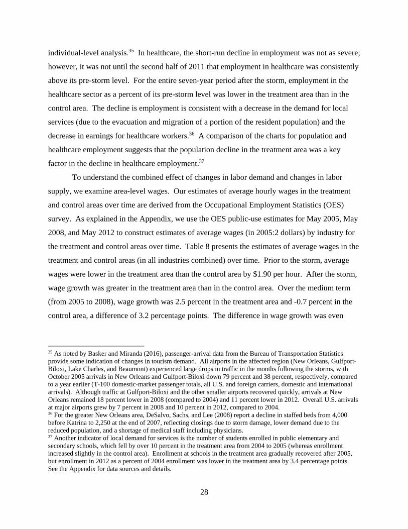
28

individual-level analysis.35 In healthcare, the short-run decline in employment was not as severe;

however, it was not until the second half of 2011 that employment in healthcare was consistently

above its pre-storm level. For the entire seven-year period after the storm, employment in the

healthcare sector as a percent of its pre-storm level was lower in the treatment area than in the

control area. The decline is employment is consistent with a decrease in the demand for local

services (due to the evacuation and migration of a portion of the resident population) and the

decrease in earnings for healthcare workers.36 A comparison of the charts for population and

healthcare employment suggests that the population decline in the treatment area was a key

factor in the decline in healthcare employment.37

To understand the combined effect of changes in labor demand and changes in labor

supply, we examine area-level wages. Our estimates of average hourly wages in the treatment

and control areas over time are derived from the Occupational Employment Statistics (OES)

survey. As explained in the Appendix, we use the OES public-use estimates for May 2005, May

2008, and May 2012 to construct estimates of average wages (in 2005:2 dollars) by industry for

the treatment and control areas over time. Table 8 presents the estimates of average wages in the

treatment and control areas (in all industries combined) over time. Prior to the storm, average

wages were lower in the treatment area than the control area by $1.90 per hour. After the storm,

wage growth was greater in the treatment area than in the control area. Over the medium term

(from 2005 to 2008), wage growth was 2.5 percent in the treatment area and -0.7 percent in the

control area, a difference of 3.2 percentage points. The difference in wage growth was even

35 As noted by Basker and Miranda (2016), passenger-arrival data from the Bureau of Transportation Statistics provide some indication of changes in tourism demand. All airports in the affected region (New Orleans, Gulfport-Biloxi, Lake Charles, and Beaumont) experienced large drops in traffic in the months following the storms, with October 2005 arrivals in New Orleans and Gulfport-Biloxi down 79 percent and 38 percent, respectively, compared to a year earlier (T-100 domestic-market passenger totals, all U.S. and foreign carriers, domestic and international arrivals). Although traffic at Gulfport-Biloxi and the other smaller airports recovered quickly, arrivals at New Orleans remained 18 percent lower in 2008 (compared to 2004) and 11 percent lower in 2012. Overall U.S. arrivals at major airports grew by 7 percent in 2008 and 10 percent in 2012, compared to 2004. 36 For the greater New Orleans area, DeSalvo, Sachs, and Lee (2008) report a decline in staffed beds from 4,000 before Katrina to 2,250 at the end of 2007, reflecting closings due to storm damage, lower demand due to the reduced population, and a shortage of medical staff including physicians. 37 Another indicator of local demand for services is the number of students enrolled in public elementary and secondary schools, which fell by over 10 percent in the treatment area from 2004 to 2005 (whereas enrollment increased slightly in the control area). Enrollment at schools in the treatment area gradually recovered after 2005, but enrollment in 2012 as a percent of 2004 enrollment was lower in the treatment area by 3.4 percentage points. See the Appendix for data sources and details.

29

greater over the long term: wage growth from 2005 to 2012 was 6.9 percent in the treatment area

and 0.9 percent in the control area, a difference of 6.0 percentage points.

6.2. Interpretation of Labor-Market Evidence

The framework presented in Section 2 and the empirical evidence on changes in average

wages both in the aggregate and by sector provide us a means to evaluate whether local labor-

market dynamics can explain the long-term increase in earnings of individuals in the treatment

sample relative to the control sample. As outlined in Section 2, workers in non-tradable

industries related to rebuilding are likely to experience an increase in both wages and average

earnings due to an increase in demand. For workers in non-tradable sectors unrelated to

rebuilding, the effects on workers’ wages and average earnings are ambiguous. If the shift to the

left of the labor-hour demand curve is larger than the shift to the left of the labor-hour supply

curve, wages will fall. Correspondingly, average earnings for workers initially employed in the

sector will decline. We anticipate that this type of shift would be most likely for non-tradable

sectors tied to the size of the local population such as health care or public/education.

Alternatively, if the shift to the left of the labor-hours supply curve is larger than the shift to the

left of the labor-hours demand curve in a non-tradable sector unrelated to rebuilding, wages will

rise. The average earnings of workers in these sectors, however, could rise, fall, or remain the

same.38 We anticipate that this type of shift would be most likely in sectors such as

leisure/accommodations, which has a component of demand related to non-residents coming to

the area.

At the aggregate level (across all sectors), the time pattern and magnitude of the area-

level estimates of average wages in treatment and control areas provide strong evidence that an

increase in relative wages in the affected area was an important factor behind the long-term

earnings gains experienced by affected individuals in our individual-level analysis. Over the

medium term (2005 to 2008), wage growth was higher in the treatment area by 3.2 percentage

points (Table 8) and affected individuals experienced an earnings gain of 3.5 percent of pre-

storm earnings (Table 6). Over the long term (2005 to 2012), wage growth was higher in the 38 Our estimates of earnings effects by industry are based on workers’ pre-storm industry. Because average earnings are calculated using all individuals employed in the industry prior to the storm and workers who are not employed after the storm are assigned zero hours, average earnings unambiguously decline when the inward shift of the labor-hours demand curve is greater than the inward shift of the labor-hours supply curve. However, for inward shifts of the labor-hour demand and supply curves that result in a wage increase, earnings for all workers initially employed in the industry will be ambiguous.

30

treatment area by 6.0 percentage points (Table 8) and affected individuals experienced an

earnings gain of 8.0 percent of pre-storm earnings (Table 6). Further, wage gains being the

primary cause of higher earnings among workers in our treatment sample is consistent with our

decomposition estimates, which demonstrate that earning gains are caused primarily by within-

employment shifts.

In addition to the aggregate evidence, variation by industry sector supports this

explanation. Figure 8 plots wage growth in the treatment area (relative to the control area) and

earnings growth in the treatment sample (relative to the control sample) from 2005 to 2012, by

industry sector. Across sectors, the magnitude of wage growth (from the area-level estimates) is

positively correlated with the magnitude of long-term effects of the storm on earnings (from the

individual-level estimates).39 Stated another way, the sectors with stronger growth in relative

wages tend to be the sectors with stronger earnings gains in our individual-level analysis. These

sectors include construction, manufacturing, and agriculture/natural resources. By contrast,

healthcare and public/education had weaker growth in relative wages in the treatment area and

weaker earnings gains in our individual-level analysis.

7. Conclusion

This study contributes to our knowledge of mass disasters by examining the employment

and earnings of individuals affected by Hurricanes Katrina and Rita. We find that these

hurricanes reduced the earnings of affected individuals in the immediate aftermath of the storms

and over the first year after the storms. The earnings losses, which were due primarily to shifts

to non-employment, reflect various aspects of the short-run disruption caused by the hurricanes.

Physical damages brought about by the storms forced some affected individuals to take up

temporary residence in other areas, causing them to take leave from or separate from their pre-

storm jobs. Many businesses closed or reduced their operations in the aftermath of the storm,

due to storm damage or reductions in demand for their output. Our results indicate that

individuals whose residence or workplace suffered damage experienced larger earnings losses in

the short term. Short-term earnings losses were also more severe for those who moved to a

39 This relationship also holds over the medium term (2005 to 2008).

31

different area during the first year after the storm and for those who separated from their pre-

storm jobs.

Although the hurricanes caused earnings losses in the short term, on average they led to

earnings gains in the medium term and long term. These gains are primarily the result of

increases in earnings within employment. We provide evidence that the long-term earnings

gains experienced by affected individuals were the result of differences in local labor-market

dynamics between the affected areas and the control areas. Area-level data on population,

employment, and average wages suggest that in the affected areas labor supply decreased and

labor demand increased—producing an increase in relative wages in the affected areas. The

magnitude of this increase in wages at the area level is comparable to the magnitude of the

earnings gains we estimate in our individual-level analysis. Variation by industry sector

provides additional support for this explanation for the long-term earnings gains.

After Hurricanes Katrina and Rita, the long-term earnings gains were widespread but the

short-term earnings losses were concentrated in particular subgroups. On average over the entire

post-storm period (when both short-term losses and long-term gains are considered), we find that

the storm led to a net increase in the average quarterly earnings of affected individuals.

However, for some subgroups the storm led to no net change or a net decrease in average

quarterly earnings: those who relocated during the first year after the storm, those who separated

from their pre-storm employer during the first year after the storm, those whose residence or

workplace experienced damage, and those who worked in sectors closely tied to tourism or the

size of the local population. These subgroups experienced earnings losses in the aftermath of the

storms that were more severe and persistent than those experienced by other affected individuals.

Relating to the literature on regional adjustments (e.g., Blanchard and Katz, 1992),

natural disasters are often studied in a growth context, with interest from macroeconomic,

regional, and development perspectives on the persistence and propagation of a local shock

(Cavallo and Noy, 2011; Strobl, 2011). Our findings help to explain the pathways at work in an

affected local labor market, which provides insight into the role of regional and inter-industry

earnings and wage differentials during a recovery period. We also provide a new perspective on

disasters by focusing on long-run outcomes of those affected and the determinants of disparities

in outcomes.

32

Regarding regional outcomes, Belasen and Polachek (2009) theorize that a destructive

shock perceived to be temporary is likely to negatively affect labor supply while having an

indeterminate effect on labor demand. Using aggregate data from Florida, they find that

hurricanes reduce employment and increase earnings in directly-affected counties in the quarter

after impact (Belasen and Polachek, 2008, 2009), though they also find variation by industry.

Others, examining hurricanes and floods with varying intensity, context, and data, find a range of

effects on local labor markets (e.g., Dolfman, Wasser, and Bergman, 2007; Coffman and Noy,

2011; Xiao, 2011). One concern with interpreting these aggregate outcomes is the extent to

which earnings changes reflect gains for directly-affected workers versus selectivity in entry and

exit from local employment. In our study, we find long-run earnings gains both overall and for

non-migrants (those most likely to work locally). We confirm that earnings gains are attributable

to higher pay within jobs and we corroborate these earnings results with aggregate wage data at

an industry level. Our finding of substantial earnings gains in the construction industry suggests

that, whatever the role of worker inflows, local workers contributed significantly to rebuilding.

Furthermore, our finding of substantial disparities in the earnings outcomes across industries

suggests that the industry composition of an affected labor market may help to determine the

overall path of earnings recovery.

Little is known about long-run effects of disasters on individuals’ earnings, even though

quantifying earnings outcomes would be important for assessing welfare consequences. One of

the only comparable studies, also covering Hurricane Katrina (Deryugina et al., 2014), finds a

similar pattern of long-run earnings gains for affected workers but lacks the employer, industry,

and quarterly-earnings data to track as wide a range of labor-market outcomes. Long-run studies

for earthquakes in Indonesia (Gignoux and Menéndez, 2016; Kirchberger, 2017) also find

earnings gains for directly-affected workers, though in a very different context. We find that

overall long-run earnings gains for affected workers mask wide disparities depending on the

damage to a worker’s pre-storm residence or workplace and on pre-storm industry sector. There

has been extensive research on long-run effects of mass-displacement events (Jacobson et al.,

1993) and import competition (Autor, Dorn, and Hanson, 2013) that has been informative of

labor-market mechanics as well as significant events and ongoing trends. We find that natural

disasters can have similar disruptive effects on workers depending on their circumstances.

33

More generally, our study demonstrates that disasters may have both direct and indirect

effects on individuals. Direct effects include the damages to residences and workplaces as well

as impacts on individuals’ physical and mental health. Indirect effects include changes in wages

and prices that are caused by disasters and rebuilding through changes in labor, product, and

housing markets. Although the direct effects are more obvious in the immediate aftermath of a

disaster, the indirect effects ultimately may have greater overall economic impact.

34

8. References

Abadie, A., A. Diamond, and J. Hainmueller. 2010. “Synthetic Control Methods for Comparative Case Studies: Estimating the Effect of California’s Tobacco Control Program.” Journal of the American Statistical Association 105(490): 493-505. Abowd, J.M., B. Stephens, L. Vilhuber, F. Andersson, K. McKinney, M. Roemer, and S. Woodcock. 2009. “The LEHD Infrastructure Files and the Creation of the Quarterly Workforce Indicators,” in T. Dunne, J.B. Jensen, and M.J. Roberts, eds., Producer Dynamics: New Evidence from Micro Data. Chicago: University of Chicago Press for the National Bureau of Economic Research, pp. 149-230. Angrist, J.D., and J.S. Pischke. 2009. Mostly Harmless Econometrics: An Empiricist’s Companion. Princeton, NJ: Princeton University Press. Austin, P.C. 2009. “Balance Diagnostics for Comparing the Distribution of Baseline Covariates between Treatment Groups in Propensity Score Matched Samples.” Statistics in Medicine 28(25): 3083-3107. Autor, D.H., D. Dorn, and G.H. Hanson. 2013. “The China Syndrome: Local Labor Market Effects of Import Competition in the United States.” American Economic Review 103(6): 2121-2168. Basker, E., and J. Miranda. 2016. “Taken by Storm: Business Financing and Survival in the Aftermath of Hurricane Katrina.” Working Paper CES 14-20. Washington, DC: Center for Economic Studies, U.S. Census Bureau. Belasen, A.R., and S.W. Polachek. 2008. “How Hurricanes Affect Wages and Employment in Local Labor Markets.” American Economic Review 98(2): 49-53. Belasen, A.R., and S.W. Polachek. 2009. “How Disasters Affect Local Labor Markets: The Effects of Hurricanes in Florida.” Journal of Human Resources 44(1): 251-276. Blake, E.S., C.W. Landsea, and E.J. Gibney. 2011. The Deadliest, Costliest, and Most Intense United States Tropical Cyclones from 1851 to 2010. Miami, FL: National Hurricane Center. Blanchard, O.J., and L.F. Katz. 1992. “Regional Evolutions.” Brookings Papers on Economic Activity 1:1-61. Brown, S.P., and P. Carey. 2006. “Mass Layoff Statistics Program: Response and Findings.” Monthly Labor Review 129(8): 70-75. Brown, S.P., S.L. Mason, and R.B. Tiller. 2006. “The Effect of Hurricane Katrina on Employment and Unemployment.” Monthly Labor Review 129(8): 52-69.

35

Caballero, R.J., and M.L. Hammour. 1994. “The Cleansing Effect of Recessions.” American Economic Review 84(5): 1350-1368. Cameron, A. Colin, and Douglas L. Miller. 2015. “A Practitioner’s Guide to Cluster-Robust Inference.” Journal of Human Resources 50(2): 317-372. Cavallo, Eduardo, and Ilan Noy. 2011. “Natural Disasters and the Economy—A Survey.” International Review of Environmental and Resource Economics 5(1): 63-102. Clayton, R.L. and J.R. Spletzer. 2006. “Worker Mobility Before and After Hurricane Katrina.” Monthly Labor Review 129(8): 11-21. Coffman, Makena, and Ilan Noy. 2012. “Hurricane Iniki: Measuring the Long-Term Economic Impact of a Natural Disaster Using Synthetic Control.” Environment and Development Economics 17(2): 187-205. Congressional Budget Office. 2005. “The Macroeconomic and Budgetary Effects of Hurricanes Katrina and Rita: An Update.” September 29, 2005. Congressional Budget Office. 2007. “The Federal Government’s Spending and Tax Actions in Response to the 2005 Gulf Coast Hurricanes.” August 1, 2007. Cutter, S.L., C.T. Emrich, J.T. Mitchell, B.J. Boruff, M. Gall, M.C. Schmidtlein, C.G. Burton, and G. Melton. 2006. “The Long Road Home: Race, Class, and Recovery from Hurricane Katrina.” Environment 48(2): 8-20. Deryugina, T., L. Kawano, and S. Levitt. 2014. “The Economic Impact of Hurricane Katrina on its Victims: Evidence from Individual Tax Returns.” Working Paper 20713. Cambridge, MA: National Bureau of Economic Research. DeSalvo, K.B., B.P. Sachs, and L. Lee. 2008. “Health Care Infrastructure in Post-Katrina New Orleans: A Status Report.” American Journal of the Medical Sciences 336(2): 197-200. De Silva, D.G., R.P. McComb, Y. Moh, A. Schiller, and A.J. Vargas. 2010. “The Effect of Migration on Wages: Evidence from a Natural Experiment.” American Economic Review 100(2): 321-326. Dolfman, M.L., S.F. Wasser, and B. Bergman. 2007. “The Effects of Hurricane Katrina on the New Orleans Economy.” Monthly Labor Review 130(3): 3-18. Elliott, J.R., and J. Pais. 2006. “Race, Class, and Hurricane Katrina: Social Differences in Human Response to Disaster.” Social Science Research 35(2): 295-321. Fallick, B.C. 1996. “A Review of the Recent Empirical Literature on Displaced Workers.” Industrial and Labor Relations Review 50(1): 5-16.

36

Federal Emergency Management Agency [FEMA]. 2005. “FEMA Mapping and Analysis, Hurricane Katrina, Remote Sensing Data from National Geospatial-Intelligence Agency.” Gallagher, J., and D. Hartley. 2017. “Household Finance after a Natural Disaster: The Case of Hurricane Katrina.” American Economic Journal: Economic Policy 9(3): 199-228. Gignoux, Jérémie, and Marta Menéndez. 2016. “Benefit in the Wake of Disaster: Long-Run Effects of Earthquakes on Welfare in Rural Indonesia.” Journal of Development Economics 118: 26-44. Gregory, J. 2014. “The Impact of Post-Katrina Rebuilding Grants on the Resettlement Choices of New Orleans Homeowners.” Unpublished Manuscript. Groen, J.A., and A.E. Polivka. 2008a. “Hurricane Katrina Evacuees: Who They Are, Where They Are, and How They Are Faring.” Monthly Labor Review 131(3): 32-51. Groen, J.A., and A.E. Polivka. 2008b. “The Effect of Hurricane Katrina on the Labor Market Outcomes of Evacuees.” American Economic Review 98(2): 43-48. Groen, J.A., and A.E. Polivka. 2010. “Going Home after Hurricane Katrina: Determinants of Return Migration and Changes in Affected Areas.” Demography 47(4): 821-844. Hallegatte, S., and P. Dumas. 2008. “Can Natural Disasters Have Positive Consequences? Investigating the Role of Embodied Technical Change.” Ecological Economics 68(3): 777-786. Hartwig, R.P., and C. Wilkinson. 2010. “Hurricane Katrina: The Five Year Anniversary.” Insurance Information Institute. http://www.iii.org/sites/default/files/docs/pdf/1007Katrina5Anniversary.pdf (accessed August 14, 2015). Hunter, L.M. 2005. “Migration and Environmental Hazards.” Population and Environment 26(4): 273-302. Jarmin, R.S., and J. Miranda. 2009. “The Impact of Hurricanes Katrina, Rita, and Wilma on Business Establishments.” Journal of Business Valuation and Economic Loss Analysis 4(2): Article 7. Jacobson, L.S., R.J. LaLonde, and D.G. Sullivan. 1993. “Earnings Losses of Displaced Workers.” American Economic Review 84(4): 685-709. Kirchberger, Martina. 2017. “Natural Disasters and Labor Markets.” Journal of Development Economics 125: 40-58. Knabb, R.D., J.R. Rhome, and D.P. Brown. 2005. Tropical Cyclone Report: Hurricane Katrina. Miami, FL: National Hurricane Center.

37

Knabb, R.D., D.P. Brown, and J.R. Rhome. 2006. Tropical Cyclone Report: Hurricane Rita. Miami, FL: National Hurricane Center. Kosanovich, K. 2006. “The Labor Market Impact of Hurricane Katrina: An Overview.” Monthly Labor Review 129(8): 3-10. Marchand, J. 2012. “Local Labor Market Impacts of Energy Boom-Bust-Boom in Western Canada.” Journal of Urban Economics 71(1): 165-174. McIntosh, M.F. 2008. “Measuring the Labor Market Impacts of Hurricane Katrina Migration: Evidence from Houston, Texas.” American Economic Review 98(2): 54-57. National Oceanic and Atmospheric Administration. 2013. NOAA’s List of Coastal Counties for the Bureau of the Census Statistical Abstract Series. https://www.census.gov/geo/landview/lv6help/coastal_cty.pdf (accessed May 24, 2013). Nordhaus, W.D. 2010. “The Economics of Hurricanes and Implications of Global Warming.” Climate Change Economics 1(1): 1-20. Okuyama, Y. 2003. “Economics of Natural Disasters: A Critical Review.” Research Paper 2003-12. West Virginia University, Regional Research Institute. Paxson, C., E. Fussell, J. Rhodes, and M. Waters. 2012. “Five Years Later: Recovery from Post Traumatic Stress and Psychological Distress among Low-Income Mothers Affected by Hurricane Katrina.” Social Science and Medicine 74(2): 150-157. Paxson, C., and C.E. Rouse. 2008. “Returning to New Orleans after Hurricane Katrina.” American Economic Review 98(2): 38-42. Plyer, A., E. Ortiz, B. Horwitz, and G. Hobor. 2013. The New Orleans Index at Eight: Measuring Greater New Orleans’ Progress toward Prosperity. New Orleans, LA: New Orleans Community Data Center. Sacerdote, B. 2012. “When the Saints Go Marching Out: Long-Term Outcomes for Student Evacuees from Hurricanes Katrina and Rita.” American Economic Journal: Applied Economics 4(1): 109-135. Sastry, N. 2009. “Tracing the Effects of Hurricane Katrina on the Population of New Orleans: The Displaced New Orleans Residents Pilot Study.” Sociological Methods and Research 38(1): 171-196. Sisk, B., and C.L. Bankston III. 2014. “Hurricane Katrina, a Construction Boom, and a New Labor Force: Latino Immigrants and the New Orleans Construction Industry, 2000 and 2006-2010.” Population Research and Policy Review 33(3): 309-334.

38

Sommers, B.D., S.K. Long, and K. Baicker. 2014. “Changes in Mortality after Massachusetts Health Care Reform: A Quasi-experimental Study.” Annals of Internal Medicine 160(9): 585-593. Stevens, D. 2007. “Employment That Is Not Covered By State Unemployment Insurance Laws.” Longitudinal Employer-Household Dynamics Technical Paper No. TP-2007-04. Strobl, E. 2011. “The Economic Growth Impact of Hurricanes: Evidence from U.S. Coastal Counties.” Review of Economics and Statistics 93(2): 575-589. Tolbert, C.M., and M. Sizer. 1996. “U.S. Commuting Zones and Labor Market Areas: A 1990 Update.” Economic Research Service Staff Paper No. 9614. U.S. Department of Housing and Urban Development [HUD]. 2006. Current Housing Unit Damage Estimates: Hurricanes Katrina, Rita, and Wilma. Washington, DC: U.S. Department of Housing and Urban Development, Office of Policy Development and Research. Vey, J.S. 2007. Restoring Prosperity: The State Role in Revitalizing America’s Older Industrial Cities. Washington, DC: Brookings Institution. Vigdor, J.L. 2007. “The Katrina Effect: Was There a Bright Side to the Evacuation of Greater New Orleans?” B.E. Journal of Economic Analysis and Policy, Advances, 7(1): Article 64. Vigdor, J. 2008. “The Economic Aftermath of Hurricane Katrina.” Journal of Economic Perspectives 22(4): 135-154. Womble, J.A., S. Ghosh, B.J. Adams, and C.J. Friedland. 2006. Advanced Damage Detection for Hurricane Katrina: Integrated Remote Sensing and VIEWS Field Reconnaissance. Buffalo, NY: Multidisciplinary Center for Earthquake Engineering Research. Xiao, Yu. 2011. “Local Economic Impacts of Natural Disasters.”Journal of Regional Science 51(4): 804-820. Zissimopoulos, J., and L.A. Karoly. 2010. “Employment and Self-employment in the Wake of Hurricane Katrina.” Demography 47(2): 345-367.

39

Table 1. Summary Statistics for Treatment and Control Samples

Variable Treatment Potential

Control Matched Control

Male 50.1 50.9 49.0 Female 49.9 49.1 51.0 25 ≤ Age < 30 12.9 14.0 12.5 30 ≤ Age < 40 29.4 29.0 30.3 40 ≤ Age < 50 33.6 32.8 33.1 50 ≤ Age < 60 24.1 24.2 24.1 White, not Hispanic 64.7 72.5 64.9 Black, not Hispanic 27.1 9.9 26.9 Hispanic 5.3 11.0 4.5 Other race, not Hispanic 2.9 6.6 3.7 Less than high school 12.4 9.5 11.0 High school 32.3 27.6 31.3 Some college 32.9 32.7 32.0 College 22.3 30.2 25.7 Annual earnings < $23K 36.7 28.9 34.8 $23K ≤ Annual earnings < $43.5K 33.5 34.7 35.6 Annual earnings ≥ $43.5K 29.8 36.5 29.7 Agriculture and resources 3.0 1.2 1.8 Construction 6.8 5.3 6.0 Manufacturing 12.7 15.1 13.8 Leisure, Accommodations 7.5 5.4 6.2 Healthcare 14.5 13.4 13.8 Professional services 12.7 17.0 14.1 Local services 17.0 16.6 17.4 Trade, Transport, Utilities 9.6 9.6 10.6 Public, Education 16.2 16.3 16.3 Earnings 2003:3 8,706 10,187 9,214 Earnings 2003:4 9,428 11,228 10,001 Earnings 2004:1 9,104 10,952 9,821 Earnings 2004:2 9,040 10,721 9,620 Earnings 2004:3 9,161 10,797 9,701 Earnings 2004:4 10,015 12,021 10,618 Earnings 2005:1 9,698 11,456 10,361 Earnings 2005:2 9,916 11,523 10,388 Percent employed, 2005:2 50.7 58.0 53.3 Unemployment rate, 2004 6.2 5.6 6.1 Housing-price change, 2000:2-2005:2 23.8 37.4 22.7 Population change, 2000-2005 3.7 3.7 5.2 Observations 138,000 8,124,000 406,000 Notes: Person records are drawn from the 2000 Census and ACS microdata and matched to LEHD quarterly earnings records. Demographic variables including sex, age (in 2005), race, ethnicity, and educational attainment are derived from the survey data. Earnings (in 2005:2 dollars) and industry variables are derived from LEHD earnings and employer records. Annual earnings are based on the eight quarters before the storm, 2003:3–2005:2. Statistics on attachment, unemployment, housing prices, and population change are for pre-storm county of residence. See Appendix for industry definitions.

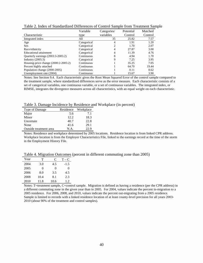
40

Table 2. Index of Standardized Differences of Control Sample from Treatment Sample

Characteristic Variable type

Categories/ variables

Potential Control

Matched Control

Integrated index All 35 25.82 7.57 Age Categorical 4 1.91 1.20 Sex Categorical 2 1.70 2.07 Race/ethnicity Categorical 4 27.87 3.00 Educational attainment Categorical 4 11.39 4.76 Quarterly earnings (2003:3-2005:2) Continuous 8 4.94 1.70 Industry (2005:3) Categorical 9 7.25 3.95 Housing-price change (2000:2-2005:2) Continuous 1 35.25 7.05 Percent highly attached Continuous 1 64.70 19.44 Population change (2000-2005) Continuous 1 0.11 8.62 Unemployment rate (2004) Continuous 1 15.67 3.90 Notes: See Section 9.4. Each characteristic gives the Root Mean Squared Error of the control sample compared to the treatment sample, where standardized differences serve as the error measure. Each characteristic consists of a set of categorical variables, one continuous variable, or a set of continuous variables. The integrated index, or RIMSE, integrates the divergence measures across all characteristics, with an equal weight on each characteristic. Table 3. Damage Incidence by Residence and Workplace (in percent) Type of Damage Residence Workplace Major 5.6 7.1 Minor 12.2 18.3 Uncertain 40.7 22.8 None 41.6 29.1 Outside treatment area N.A. 22.9 Notes: Residence and workplace determined by 2005 locations. Residence location is from linked CPR address. Workplace location is from the Employer Characteristics File, linked to the earnings record at the time of the storm in the Employment History File. Table 4. Migration Outcomes (percent in different commuting zone than 2005) Year T C T – C 2004 3.0 4.5 -1.5 2005 0 0 0 2006 8.0 3.5 4.5 2008 10.4 8.1 2.3 2010 11.8 10.6 1.2 Notes: T=treatment sample, C=control sample. Migration is defined as having a residence (per the CPR address) in a different commuting zone in the given year than in 2005. For 2004, values indicate the percent in-migration to a 2005 residence. For 2006, 2008, and 2010, values indicate the percent out-migrating from a 2005 residence. Sample is limited to records with a linked residence location of at least county-level precision for all years 2003-2010 (about 90% of the treatment and control samples).

41

Table 5. Effects on Earnings, Overall and by Damage Type Effects by Time Period after the Storm

Short Medium Long Full All -298.4 343.0* 792.3* 403.8* (191.4) (125.4) (141.8) (127.9) [-3.0] [3.5] [8.0] [4.1] Residence Damage Major -1,710.3* -302.6 535.2* -295.8*

(322.2) (159.8) (181.0) (141.7) [-17.2] [-3.1] [5.4] [-3.0] Minor -631.9* 295.0* 772.1* 258.8

(167.9) (120.3) (258.9) (134.9) [-6.4] [3.0] [7.8] [2.6] Uncertain -59.1 433.1* 822.7* 505.5* (122.3) (114.9) (159.1) (118.8) [-0.6] [4.4] [8.3] [5.1] None -245.4 355.5* 802.9* 440.6*

(210.0) (157.2) (158.3) (149.2) [-2.5] [3.6] [8.1] [4.4] Workplace Damage Major -1,444.0* -2.7 835.9* 41.4

(252.9) (121.9) (226.5) (129.1) [-14.6] [0.0] [8.4] [0.4] Minor -755.3* 286.1 754.7* 218.7

(298.2) (171.9) (189.6) (181.6) [-7.6] [2.9] [7.6] [2.2] Uncertain -40.9 432.0* 928.6* 573.6* (124.7) (123.6) (172.7) (124.4) [-0.4] [4.4] [9.4] [5.8] None -214.8 232.4 629.0* 323.6*

(192.1) (174.8) (157.7) (135.7) [-2.2] [2.3] [6.3] [3.3] Outside treatment area 57.5 546.8* 880.8* 596.4

(144.5) (163.2) (171.3) (149.8) [0.6] [5.5] [8.9] [6.0]

Notes: The estimates for overall treatment effects, residence damage, and workplace damage are based on separate regressions. Numbers in parentheses are standard errors clustered at the county level (based on 2005 residence location). Numbers in brackets are effects as a percent of average earnings in 2005:2 for the treatment sample as a whole. Short term is 2005:4–2006:3 (k=1–4), medium term is 2007:4–2008:3 (k=9–12), long term is 2011:4–2012:3 (k=25–28), and full is 2005:4–2012:3 (k=1–28). * p<0.05.

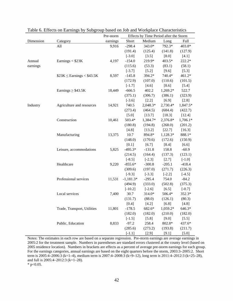
42

Table 6. Effects on Earnings by Subgroup based on Job and Workplace Characteristics Pre-storm Effects by Time Period after the Storm Dimension Category earnings Short Medium Long Full

All 9,916 -298.4 343.0* 792.3* 403.8* (191.4) (125.4) (141.8) (127.9) [-3.0] [3.5] [8.0] [4.1]

Annual Earnings < $23K 4,197 -154.0 219.9* 403.5* 222.2* earnings (115.6) (53.3) (83.1) (58.1)

[-3.7] [5.2] [9.6] [5.3] $23K ≤ Earnings < $43.5K 8,597 -145.8 394.2* 740.4* 461.2*

(172.9) (107.0) (110.6) (101.5) [-1.7] [4.6] [8.6] [5.4]

Earnings ≥ $43.5K 18,449 -666.5 402.2 1,269.2* 522.7 (375.1) (306.7) (386.1) (323.9) [-3.6] [2.2] [6.9] [2.8]

Industry Agriculture and resources 14,921 740.5 2,048.3* 2,730.4* 1,847.5* (273.4) (464.5) (684.4) (422.7) [5.0] [13.7] [18.3] [12.4]

Construction 10,461 503.4* 1,384.7* 2,376.8* 1,706.1* (180.8) (194.8) (268.0) (201.2) [4.8] [13.2] [22.7] [16.3]

Manufacturing 13,375 10.7 894.8* 1,128.3* 888.1* (148.0) (170.6) (172.6) (150.9) [0.1] [6.7] [8.4] [6.6]

Leisure, accommodations 5,825 -495.3* -131.8 158.8 -60.9 (214.5) (164.4) (137.3) (123.1) [-8.5] [-2.3] [2.7] [-1.0]

Healthcare 9,220 -855.6* -300.8 -205.1 -418.4 (309.6) (197.0) (271.7) (226.3) [-9.3] [-3.3] [-2.2] [-4.5]

Professional services 11,531 -1,181.3* -295.4 754.0 -84.2 (494.9) (333.0) (502.8) (375.3) [-10.2] [-2.6] [6.5] [-0.7]

Local services 7,400 30.7 314.0* 506.4* 352.3* (131.7) (88.0) (126.1) (80.3) [0.4] [4.2] [6.8] [4.8]

Trade, Transport, Utilities 11,801 -178.5 682.6* 1,059.2* 646.3* (182.0) (182.0) (210.0) (182.0) [-1.5] [5.8] [9.0] [5.5]

Public, Education 8,833 -97.2 258.4 802.8* 437.6* (285.6) (273.2) (193.8) (211.7) [-1.1] [2.9] [9.1] [5.0]

Notes: The estimates in each row are based on a separate regression. Pre-storm earnings are average earnings in 2005:2 for the treatment sample. Numbers in parentheses are standard errors clustered at the county level (based on 2005 residence location). Numbers in brackets are effects as a percent of average pre-storm earnings for each group. For the earnings categories, annual earnings are based on the eight quarters before the storm, 2003:3–2005:2. Short term is 2005:4–2006:3 (k=1–4), medium term is 2007:4–2008:3 (k=9–12), long term is 2011:4–2012:3 (k=25–28), and full is 2005:4–2012:3 (k=1–28). * p<0.05.

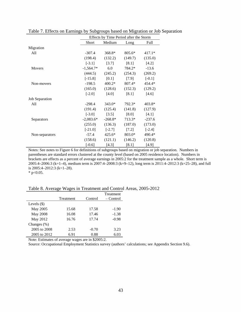
43

Table 7. Effects on Earnings by Subgroups based on Migration or Job Separation Effects by Time Period after the Storm

Short Medium Long Full Migration All -307.4 368.8* 805.6* 417.1*

(198.4) (132.2) (149.7) (135.0) [-3.1] [3.7] [8.1] [4.2] Movers -1,564.7* 6.0 784.2* -13.6

(444.5) (245.2) (254.3) (269.2) [-15.8] [0.1] [7.9] [-0.1] Non-movers -198.5 400.2* 807.4* 454.4*

(165.0) (128.6) (152.3) (129.2) [-2.0] [4.0] [8.1] [4.6]

Job Separation All -298.4 343.0* 792.3* 403.8* (191.4) (125.4) (141.8) (127.9) [-3.0] [3.5] [8.0] [4.1] Separators -2,083.6* -268.8* 713.3* -237.6 (255.0) (136.3) (187.0) (173.0) [-21.0] [-2.7] [7.2] [-2.4] Non-separators -57.4 425.6* 803.0* 490.4* (158.6) (121.1) (146.2) (120.8) [-0.6] [4.3] [8.1] [4.9] Notes: See notes to Figure 6 for definitions of subgroups based on migration or job separation. Numbers in parentheses are standard errors clustered at the county level (based on 2005 residence location). Numbers in brackets are effects as a percent of average earnings in 2005:2 for the treatment sample as a whole. Short term is 2005:4–2006:3 (k=1–4), medium term is 2007:4–2008:3 (k=9–12), long term is 2011:4–2012:3 (k=25–28), and full is 2005:4–2012:3 (k=1–28). * p<0.05. Table 8. Average Wages in Treatment and Control Areas, 2005-2012

Treatment Control Treatment – Control

Levels ($) May 2005 15.68 17.58 -1.90 May 2008 16.08 17.46 -1.38 May 2012 16.76 17.74 -0.98 Changes (%) 2005 to 2008 2.53 -0.70 3.23 2005 to 2012 6.91 0.88 6.03 Note: Estimates of average wages are in $2005:2. Source: Occupational Employment Statistics survey (authors’ calculations; see Appendix Section 9.6).

44

Figure 1. Local Labor-Market Dynamics in Storm-Affected Area over the Long Term a. Labor-demand increase for non-tradable sector (construction)

b. Labor-demand-dominated decrease for non-tradable sector

c. Labor-supply-dominated decrease for non-tradable sector

Note: “ ” and “ ” represent labor supply and demand curves, respectively. “0” and “1” subscripts refer to initial and long-term conditions, respectively. Likewise, “ ” and “ ” represent initial and long-term equilibria, while “ ” and “ ′” as well as “ ” and “ ′” represent initial and long-term wages and labor hours.

′

′

Wag

e

Quantity of Labor Hours

′

Wag

e

Quantity of Labor Hours

′

′

Wag

e

Quantity of Labor Hours

′

45

Figure 2. Treatment and Control Areas

Notes: The estimation sample consists of workers who resided in treatment counties or control counties before the Hurricanes Katrina and Rita. Treatment counties (shaded lighter) are 63 counties in Texas, Louisiana, Mississippi, and Alabama. Control counties (shaded darker) are 287 counties in 28 states. Figure 3. Effects on Earnings

Notes: Average total earnings calculated from LEHD quarterly earnings records spanning 2003:3 to 2012:3. The storms struck in 2005:3, labeled zero. All earnings are adjusted to 2005:2 (marked by the vertical line) using the Consumer Price Index. All workers held a job at the beginning of 2005:2. Sample includes 138,000 workers in the treatment sample and 406,000 in the control sample. Equation (1) provides the model specification. Estimates capture the earnings difference between individuals in the treatment and control samples in each quarter before/after the storms, relative to this difference in the first quarter before the storm (2005:2). Dashed lines show the upper and lower bounds of 95% confidence intervals, which are based on standard errors clustered at the county level (based on 2005 residence location).

-1,500

-1,000

-500

0

500

1,000

1,500

-8 -6 -4 -2 0 2 4 6 8 10 12 14 16 18 20 22 24 26 28Quarters relative to storm

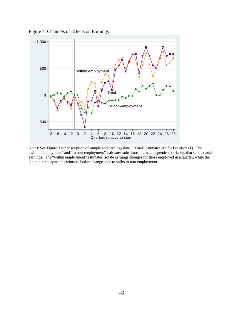
46

Figure 4. Channels of Effects on Earnings

Notes: See Figure 3 for description of sample and earnings data. “Total” estimates are for Equation (1). The “within employment” and “to non-employment” estimates substitute alternate dependent variables that sum to total earnings. The “within employment” estimates isolate earnings changes for those employed in a quarter, while the “to non-employment” estimates isolate changes due to shifts to non-employment.

To non-employment

Total

Within employment

-500

0

500

1,000

-8 -6 -4 -2 0 2 4 6 8 10 12 14 16 18 20 22 24 26 28Quarters relative to storm

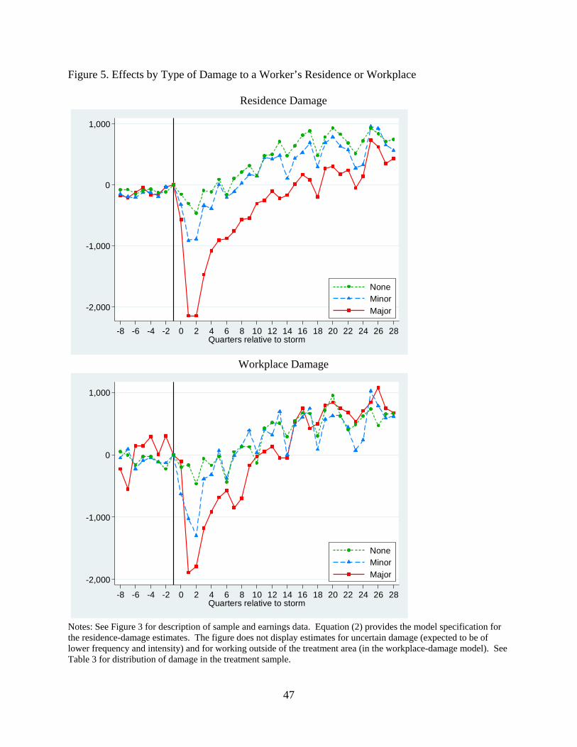
47

Figure 5. Effects by Type of Damage to a Worker’s Residence or Workplace

Residence Damage

Workplace Damage

Notes: See Figure 3 for description of sample and earnings data. Equation (2) provides the model specification for the residence-damage estimates. The figure does not display estimates for uncertain damage (expected to be of lower frequency and intensity) and for working outside of the treatment area (in the workplace-damage model). See Table 3 for distribution of damage in the treatment sample.

-2,000

-1,000

0

1,000

-8 -6 -4 -2 0 2 4 6 8 10 12 14 16 18 20 22 24 26 28Quarters relative to storm

NoneMinor

Major

-2,000

-1,000

0

1,000

-8 -6 -4 -2 0 2 4 6 8 10 12 14 16 18 20 22 24 26 28Quarters relative to storm

NoneMinor

Major

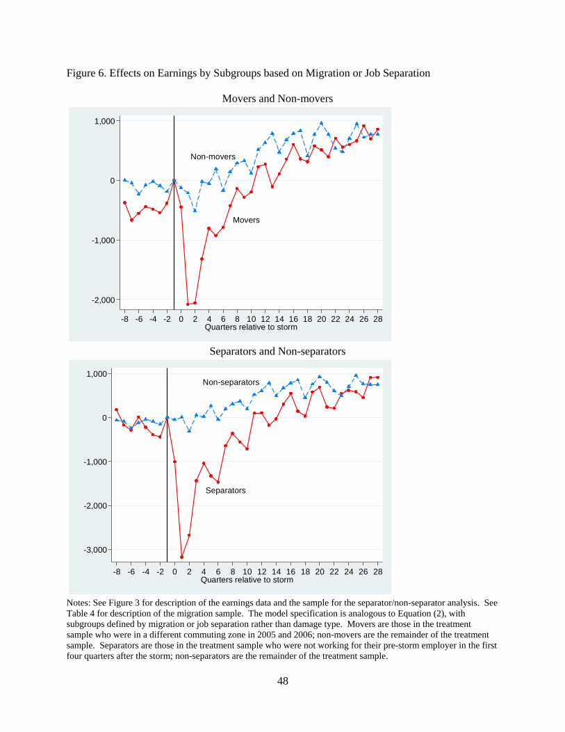
48

Figure 6. Effects on Earnings by Subgroups based on Migration or Job Separation

Movers and Non-movers

Separators and Non-separators

Notes: See Figure 3 for description of the earnings data and the sample for the separator/non-separator analysis. See Table 4 for description of the migration sample. The model specification is analogous to Equation (2), with subgroups defined by migration or job separation rather than damage type. Movers are those in the treatment sample who were in a different commuting zone in 2005 and 2006; non-movers are the remainder of the treatment sample. Separators are those in the treatment sample who were not working for their pre-storm employer in the first four quarters after the storm; non-separators are the remainder of the treatment sample.

Non-movers

Movers

-2,000

-1,000

0

1,000

-8 -6 -4 -2 0 2 4 6 8 10 12 14 16 18 20 22 24 26 28Quarters relative to storm

Non-separators

Separators

-3,000

-2,000

-1,000

0

1,000

-8 -6 -4 -2 0 2 4 6 8 10 12 14 16 18 20 22 24 26 28Quarters relative to storm

49

Figure 7. Population and Employment in Treatment and Control Areas (% of pre-storm level)

Population Employment—All Sectors

Employment—Construction Employment—Manufacturing

Employment—Leisure and Accommodations Employment—Healthcare

Source: Census Bureau County Population Estimates (public-use data) and Quarterly Workforce Indicators (authors’ calculations; see Appendix).

Control

Treatment

70

80

90

100

110

120

2000 2002 2004 2006 2008 2010 2012

Treatment

Control

70

80

90

100

110

120

2004 2005 2006 2007 2008 2009 2010 2011 2012

Treatment

Control

70

80

90

100

110

120

2004 2005 2006 2007 2008 2009 2010 2011 2012

Treatment

Control

70

80

90

100

110

120

2004 2005 2006 2007 2008 2009 2010 2011 2012

Treatment

Control

70

80

90

100

110

120

2004 2005 2006 2007 2008 2009 2010 2011 2012

Treatment

Control

70

80

90

100

110

120

2004 2005 2006 2007 2008 2009 2010 2011 2012

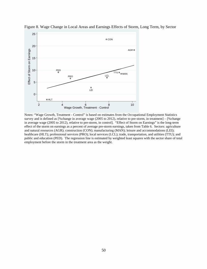
50

Figure 8. Wage Change in Local Areas and Earnings Effects of Storm, Long Term, by Sector

Notes: “Wage Growth, Treatment - Control” is based on estimates from the Occupational Employment Statistics survey and is defined as [%change in average wage (2005 to 2012), relative to pre-storm, in treatment] – [%change in average wage (2005 to 2012), relative to pre-storm, in control]. “Effect of Storm on Earnings” is the long-term effect of the storm on earnings as a percent of average pre-storm earnings, taken from Table 6. Sectors: agriculture and natural resources (AGR); construction (CON); manufacturing (MAN); leisure and accommodations (LEI); healthcare (HLT); professional services (PRO); local services (LCL); trade, transportation, and utilities (TTU); and public and education (PED). The regression line is estimated by weighted least squares with the sector share of total employment before the storm in the treatment area as the weight.

AGR

CON

MAN

LEI

HLT

PRO LCLTTU

PED

0

5

10

15

20

25

Effe

ct o

f Sto

rm o

n E

arni

ngs

2 4 6 8 10Wage Growth, Treatment - Control

51

9. Appendix 9.1 Worker Data

In order to examine longitudinal outcomes for individuals potentially affected by Hurricanes Katrina and Rita, this paper makes use of restricted-access administrative and survey data brought together at the U.S. Census Bureau. The combined dataset tracks quarterly labor-market outcomes and includes a variety of demographic variables. The structure of the combined dataset permits us to examine individuals before and after the storms and to examine storm effects over a seven-year period. The large sample size also allows us to obtain precise parameter estimates and enables us to examine subsamples of the population.

We begin with an extract from the 2000 Census long-form microdata and American Community Survey (ACS) microdata (from January 2003 to July 2005) of persons who were aged 25 to 59 in 2005 and at least 25 when they responded to the survey. The 2000 long-form, or Sample Census Edited File, contributes approximately 90 percent of the respondents overall, but the ACS provides all of the respondents under age 30 in 2005.40 The lower bound for age reduces the likelihood of non-employment reflecting college attendance and improves the likelihood that reported educational attainment reflects attainment as of 2005. The upper bound for age reduces the likelihood of retirement within the study period. From the survey responses, we obtain demographic information (age, sex, race, and ethnicity) and educational attainment. In order to match the survey records to administrative data, we make use of a unique personal identifier, called a Protected Identification Key (PIK). The Census Bureau uses federal administrative data to probabilistically match survey responses to a PIK, based on a comparison of personally identifying information.41 For this combined survey sample, approximately 90 percent of records have a PIK match.

For each person in the survey sample, we determine a pre-hurricane residential location, using a PIK-linked address file based on federal administrative records. The Census Bureau produces an annual Composite Person Record (CPR) residence file, which provides a single residence location for a PIK in a given year (Abowd et al., 2009).42 For the extract of survey respondents with a PIK, 96 percent match to a CPR record that provides at least county-level precision and 79 percent match to a Census tract and block location. Because the majority of CPR records are sourced from the addresses on federal income-tax returns (which are typically filed in the first four months of the year), the 2005 locations are a good representation of pre-storm location. We limit the sample to survey respondents with both a PIK and an administrative residence location in 2005 that is precise to the county level or better.

We reweight survey responses based on the relative prevalence of demographic characteristics at the national level in 2005 and based on the likelihood of a person having a link to the CPR with county-level geography or better.43 We use the new weights for computations reported in the paper, including summary statistics and regressions. 40 The ACS expanded its sampling by threefold in 2005, so the majority of ACS responses are from that year, even though only the first seven months are used. 41 In less than 1% of cases, multiple responses may be matched to the same PIK. In this event, we randomly retain the PIK of only one respondent. 42 The LEHD program uses residences provided in the CPR for imputations and as a place of residence for jobs data in the LEHD Origin-Destination Employment Statistics, available in the Web tool OnTheMap. 43 First, we estimate the number of 2005 persons that each survey respondent with a PIK in our age range represents (based on combinations of age, sex, and race/ethnicity categories). Then we estimate a logistic regression with the

52

We then match the survey records, by PIK, to LEHD earnings records for jobs held between 2003 quarter 3 (also denoted as 2003:3) and 2012 quarter 3 (2012:3).44 The LEHD program produces a set of microdata Infrastructure Files using employment data provided by states along with federal administrative data and survey data (Abowd et al., 2009). States that have joined the Local Employment Dynamics (LED) Partnership provide the Census Bureau with two employment files each quarter.45 Unemployment Insurance (UI) earnings records list the quarterly earnings of each worker from each of his or her employers. The LEHD program compiles the records as an Employment History File, with a record in the file for each job, identified by the combination of a worker (PIK) and employer, which is identified by a State Employer Identification Number (SEIN). An SEIN may be further linked to the Employer Characteristics File, which is produced from the same source data that employers submit to the Bureau of Labor Statistics for the Quarterly Census of Employment and Wages. The employer file lists the industry, ownership, employment, and location of establishments.

To focus our study on workers with ties to the labor market covered by LEHD data, we require that survey respondents have a job spanning July 1, 2005 (the beginning of the quarter in which the storms occurred).46 For that job (or the highest-earning one in 2005:2 if a worker had multiple such jobs), we link to the employer’s industry (NAICS code) and establishment location.47 We link over 90 percent of workers to a workplace Census tract or block, and approximately 99 percent are linked to a workplace county. We use the industry and workplace dependent variable indicating a match to a CPR residence at the county level or better and indicators for sex, age cohorts, and race/ethnicity as explanatory variables. Hispanics, younger respondents, and those with high school education or less are less likely to have a linked residence. We retain only the records with a PIK and linked residence, and we use the product of the inverse of the predicted retention probabilities from both reweighting schemes to reweight the remaining survey records. The resulting sample has very similar weighted characteristics as the original, unweighted extract. 44 The Quarterly Workforce Indicators, produced from the LEHD data, first report earnings for Mississippi in 2003:3 and first report for Texas, Louisiana, and Alabama in 1995:1, 1995:1, and 2001:1, respectively. 45 All 50 states, the District of Columbia, Puerto Rico, and the Virgin Islands joined the LED Partnership by 2012. The time series of LEHD earnings records begins in 1985, but not all states provide data in every year. By 2003, there are data for 47 states. Jobs with earnings in Arizona and the District of Columbia were not available at the beginning of the series, but they are included in later years. Jobs with earnings in Massachusetts are not included in the study. These coverage issues should have only a small effect on our analysis because the treatment and control samples do not include any individuals whose 2005 residence was in Arizona, the District of Columbia, or Massachusetts. Because Mississippi first provided earnings records for 2003:3, that quarter is the first one used in the study. 46 Using the LEHD data, we identify workers with earnings from the same employer in the adjacent quarters 2005:2 and 2005:3. The LEHD program uses this definition to tabulate beginning-of-quarter employment, with the reasoning that a worker with the same job in adjacent quarters is employed at the seam of those quarters. We use the Successor Predecessor File to span the adjacent quarters in cases where an employer identifier may have changed due to restructuring. 47 We link earnings records by SEIN to the unit-level version of the Employer Characteristics File. For jobs at single-unit employers, the link is straightforward. For jobs at multi-unit employers, we use the Unit-to-Worker (U2W) imputation, applied by the LEHD program to assign establishments to workers when establishment assignments are unknown (for all states except Minnesota). The imputation assigns an establishment to a worker only if the establishment exists during the worker’s tenure at the employer, and it uses establishment size and proximity to a worker’s place of residence as explanatory factors, attempting to replicate the size distribution of establishments and the observed distribution of commute distances. We use the first of ten draws from the imputation model. In general, the use of imputed workplace data would be expected to attenuate any estimates relating to workplace-damage measures. For our linking we use the U2W draws listed on a downstream version of the Employer History File, called the Person History File, which we also use for extracting earnings records.

53

information to examine differential effects of the storm on workers, given their pre-storm employment.

In constructing the sample for our main analysis, the July 1 job restriction reduces the sample to 57.9 percent of all the survey respondents that link to LEHD earnings histories ever over the study period (after imposing the restrictions based on age and residence data). Workers eliminated from the sample by this earnings restriction may be employed in sectors not covered by the LEHD data, including self-employment, the federal government, the postal service, the armed forces, agricultural or family work, and other non-covered sectors.48 Still, LEHD earnings records cover approximately 96 percent of private-sector, non-farm wage-and-salary employment. LEHD earnings include some high-earning records that can distort earnings measures in particular quarters. For this reason, and to focus on the earnings outcomes of typical workers, we topcode quarterly earnings levels to $500,000 (in $2005:2).

Average earnings (without any controls) for the treatment sample and the matched control sample before and after the storm are shown in Figure A5. Before the storm, average earnings is lower for the treatment sample than the control sample, but the difference in average earnings is fairly stable across quarters. In the aftermath of the storm, average earnings for the treatment sample fell relative to the control sample. However, the gap in average earnings between the treatment and control samples closed over time, and by the fourth year after the storm (2006:4) average earnings is larger in the treatment sample than in the control sample. Beyond that, average earnings is typically larger in the treatment sample.49

We define industries using 2007 NAICS Industry Sectors, as listed here by the first two digits of the code. Agriculture and resources: 11 and 21. Construction: 23. Manufacturing: 31-33. Leisure, Accommodations: 71, 72. Healthcare: 62. Professional services: 51-55. Local services: 44-45, 56, 81. Trade, Transportation, Utilities: 22, 42, 48-49. Public, Education: 61, 92. 9.2. Damage Data

The U.S. Department of Housing and Urban Development (HUD, 2006) compiled the first measure, which tabulates the number of occupied housing units in counties of Texas, Louisiana, Mississippi, and Alabama with storm damage to real and personal property. The damage assessments for Katrina and Rita were based on inspection of housing units to determine 48 See Stevens (2007) for a discussion of coverage in unemployment-insurance earnings records, which varies by state. The LEHD program is working to add data on the self-employed and on federal workers. 49 The general upward trend in quarterly earnings before the storm is due to our requirement that workers are employed at the same job in 2005:2 and 2005:3, which is associated with more weeks worked and longer job tenure in the vicinity of those quarters than earlier in the pre-storm period (when we do not require that individuals be employed). The long-run decline in average earnings for both samples is due to requiring that sample members be employed just prior to the storm (job spanning July 1, 2005) but not requiring that they be employed after the storm. The regression model compares differences in changes across the treatment and control samples relative to the baseline quarter, so the long-run decline is absorbed in the quarter effects.

54

eligibility for Federal Emergency Management Agency (FEMA) housing assistance. Inspections were either direct observations or inferences based on flood depth. For our analysis, we use the share of units in a county with “major” (between $5,200 and $29,999) or “severe” ($30,000 or higher) damage to define the treatment area (with shares based on the total number of occupied housing units according to the 2000 Census). Figure A1 maps this county-level damage share for the set of 122 counties in these four states, with darker shading indicating counties with a greater share of damaged units. The darkest regions of the map are coastal areas in the vicinity of where Katrina (in eastern Louisiana and coastal Mississippi) and Rita (in western Louisiana) made landfall.

FEMA (2005) carried out a remote-sensing analysis of 22 counties affected by Hurricanes Katrina and Rita; these counties include all of the high-damage counties (according to the data in HUD [2006]) as well as some of the moderate-damage and low-damage counties.50 This more-detailed measure is based on Geographic Information Systems (GIS) shapefiles that indicate the degree and type of damage occurring in sub-county areas defined by sets of latitude and longitude coordinates. Based on remote-sensing observations (satellite technology and airplane flyovers), FEMA designated areas as having Limited Damage, Moderate Damage, Extensive Damage, or Catastrophic Damage or being Flooded. For our sub-county analysis, we define “major damage” areas as locations with Extensive or Catastrophic Damage as well as areas in and around New Orleans with flooding that persisted beyond September 10, 2005. We define “minor damage” areas as locations with Limited or Moderate Damage as well as areas with less-persistent flooding (including New Orleans areas where flooding receded by September 10, 2005).

The survey included areas in 22 of the 63 counties in our treatment area and described the damage classifications for structures within the geographic areas as follows: Limited Damage: Generally superficial damage to solid structures (e.g., the loss of tiles or

roof shingles); some mobile homes and light structures are damaged or displaced. Moderate Damage: Solid structures sustain exterior damage (e.g., missing roofs or roof

segments); some mobile homes and light structures are destroyed, and many are damaged or displaced.

Extensive Damage: Some solid structures are destroyed, most sustain exterior damage (e.g., roofs are missing, interior walls are exposed); most mobile homes and light structures are destroyed.

Catastrophic Damage: Most solid and all light or mobile structures are destroyed. Flooded area: Area under water. Undamaged: Areas not covered by the above categories.

FEMA released several vintages of sub-county damage mapping in 2005. For this study, we use three vintages of geographic files. For Hurricane Katrina, we use both the September 10 and September 11 files. For Hurricane Rita, we use the September 29 file.51 We consider

50 Post-disaster reconnaissance includes several tiers of regional, neighborhood, and per-building assessment (Womble et al., 2006). Early stages made use of high-resolution satellite and aerial imagery. 51 Our GIS files for these snapshots have the following names: damage_10sep05_1000 (Sept. 10), katrina_receded_flooding_11sep05 (Sept. 11), and damage_29sep05_1000 (Sept. 29). FEMA released these files as events unfolded but does not maintain them or provide additional information on the creation of the files. Ron Jarmin and Javier Miranda provided the copies used here based on the data used in Jarmin and Miranda (2009).

55

flooding in the September 10 and September 29 files to be minor damage and code the flooding in the September 11 file as major damage because only those locations had long-term flooding.

For illustrative purposes, Figure A3 displays maps of two affected areas by FEMA damage category, with red indicating major damage, dark blue indicating minor damage, and green indicating land areas with no specified damage. Panel A, which depicts the New Orleans area, shows mostly flooding damage, with minor damage in the areas where flooding receded quickly and major damage in the zones where it persisted. Panel B, which depicts the Gulf coast of Mississippi, shows mostly storm surge and wind damage, with catastrophic and extensive damage directly along the coast.

For the 22 surveyed counties with detailed damage data, we identify the set of Census blocks subject to either type of damage (major or minor) and assume that the most severe damage type applies to all addresses located within each block. We regard the remainder of blocks in the surveyed counties as having no damage. For blocks in the remainder of the 63-county treatment area, damage is uncertain but likely to be of lower frequency and intensity.

To implement this mapping, we use ArcMap 10.1 (ESRI software) to intersect the damage areas of these shape files (FEMA, 2005) with TIGER/Line shapefiles for Census 2000 tabulation blocks in our treatment counties.52 A Census tract is a geographically compact and demographically homogeneous tabulation area with a target population of 4,000 residents, analogous to a neighborhood. Tracts consist of blocks, which are bounded by features such as streets, streams, and jurisdiction boundaries and often correspond with one or two city blocks in an urban area (there is no target population for a block, but there are typically dozens of blocks within a tract). Our residence addresses are geocoded to Census 2000 tabulation geography, while the workplace addresses are geocoded to Census 2010 tabulation geography. We use separate intersection files for each tabulation year to classify workers’ residences and workplaces as damaged.

For the treatment sample, Table A2 gives the distribution of damage types associated with each worker, by 2005 residence block and workplace block. The top two rows indicate addresses with positive evidence of damage. Most instances of major damage are long-term flooding or Catastrophic Damage. Minor damage is split between short-term flooding and Moderate and Limited Damage. The middle two rows indicate addresses where damage is possible but uncertain—due to either an imprecise residence or workplace address in a surveyed county or an address in a county not surveyed. All addresses for our sample are precise to at least the county level. The lower two rows indicate addresses with no damage, which were either in a surveyed county or outside the treatment area altogether (workplace only). Areas with no reported damage (shaded as green in the maps) also include sparsely populated areas that were not subject to structural damage (but may have had strong winds or flooding). Overall, 70 percent of residences and 58 percent of workplaces were within surveyed counties of the treatment area.

Figure A4 presents more-detailed views of the maps in Figure A3, overlaid with boundaries of Census blocks. Panel A shows downtown New Orleans, including the French

52 Because addresses geocoded to Census blocks are already so spatially precise, we do not make a distinction of whether an address is located in the exact part of a block that intersects with the damage shape files. One concern with a coordinate-based measure is that some addresses can be geocoded to a street of a block but cannot be precisely located along the street. Another concern is that properties extend beyond the exact coordinates of an address. Furthermore, the exact extent of damage areas may be less certain than the shape files indicate.

56

Quarter. Panel B shows an area of Gulfport, Mississippi, including beachside resorts, residential housing, and shipping terminals. Census-block boundaries are often consistent with city streets, so the maps also provide a good indication of the infrastructure layout in these areas and provide a scale for the extent of damage to urban areas. For this study, any address in a block including any minor or major damage is assumed to be subject to that damage, with major damage taking precedence over minor damage. 9.3. Pre-Storm County Characteristics for Propensity-Score Model

The propensity-score model, described in Section 3.4, includes a subset of the variables in Table 1, omitting some variables that varied little across regions and combining some categorical values of others to increase statistical power. The coefficient estimates are reported in Table A1. The primary source of the county-level characteristics for the propensity-score model is our matched survey-administrative worker data, including the requirement of continuous employment at a job from 2005:2 to 2005:3. We use these data to construct county-level means of variables for demographic characteristics (shares by race/ethnicity and educational attainment), industry composition (based on the pre-storm job), and average quarterly earnings for each of the eight quarters from 2003:3 to 2005:2.53 In the propensity-score model, agriculture and natural resources are separate categories because trends in energy prices may affect local areas differently depending on their employment shares in natural resources (Marchand, 2012). In the summary statistics in Table 1 and in our industry analysis, we combine agriculture and natural resources into a single category because there is a relatively small share of employment in each of these industries.

Given the cyclical dynamics of the 2000s, with a housing boom through 2006 and the Great Recession beginning in 2007, it is important that we match not only the population characteristics but also pre-storm economic conditions. Therefore, we include four additional county-level measures: (1) the percent of individuals who were employed just prior to the storms (defined using the same condition as our sample), (2) the unemployment rate in 2004, (3) the change in housing prices from 2000:2 to 2005:2, and (4) the change in total population from July 1, 2000, to July 1, 2005. Percent highly attached. This is the percent of individuals living in the county in 2005 who

were continuously employed at a job from 2005:2 to 2005:3. The source of this measure is our matched survey-administrative worker data.

Unemployment rate in 2004. The source of this measure is annual county-level estimates by the Bureau of Labor Statistics (Local Area Unemployment Statistics).

Housing-price change from 2000:2 to 2005:2. This measure is based on Federal Housing Finance Agency (FHFA) All-Transactions House Price Indexes, which are derived from appraisal values and sales prices. These FHFA indexes are quarterly, not seasonally adjusted, and available for 401 metropolitan areas (or metropolitan divisions) and 47 nonmetropolitan balance-of-state areas. For counties located in metropolitan areas, we use the FHFA index for that metropolitan area (or metropolitan division). For other counties, we use the FHFA index for the relevant nonmetropolitan area. The symmetric and bounded measure of change we use is 100*(hpi2005 – hpi2000) / [(hpi2000 + hpi2005)/2], where hpi2000 and hpi2005 are the index values for 2000:2 and 2005:2, respectively.

53 In calculating the means, we use person weights indicating the count of persons in 2005 represented by each record. Industry shares are based on the highest-earning job held from 2005:2 to 2005:3.

57

Population change from 2000 to 2005. This measure is based on Census Bureau population estimates at the county level, which have a reference date of July 1. The measure of change we use is 100*(p2005 – p2000) / [(p2000 + p2005)/2], where p2000 and p2005 are the population estimates for 2000 and 2005, respectively.

9.4. Control Suitability

While it is apparent from an inspection of Table 1 that the matched control sample improves upon the potential control sample in terms of alignment with the treatment sample, in Table 2 we use standardized differences to quantify the improvement. Table A8 presents the characteristics of the treatment sample, the matched control sample, and three alternate control samples. Figure A6 depicts the county composition of the three alternate control samples (described in Section 9.7). To quantify the dissimilarity of each control sample from the treatment sample, Table A9 (extending Table 2) presents a measure of how each of the control samples diverge from the treatment sample, both in the aggregate and by characteristics (each defined by a single variable or a grouping of related variables).

The standardized difference (see Austin, 2009) of any variable that is continuous at the person level (e.g., earnings, county population change from 2000 to 2005, and county unemployment rate in 2004) is calculated as

∙ ,

where is the sample mean and is the sample variance. We calculate the sample mean and variance across persons in the sample, using person weights. Note that some characteristics, such as population change, are common to all persons in the same county. The standardized difference for a categorical variable (e.g., female, age bins, and race/ethnicity categories) is calculated as

∙ ,

where is the prevalence (or mean) of a categorical variable with a value between zero and one. We compute an index of the standardized differences, a Root Mean Squared Error

(RMSE), for each characteristic as

100 ∙ ∑ ,

where is a characteristic that takes on categorical values (or consists of a set of as many continuous variables), indexed 1 to . For measuring divergence, we treat the eight pre-storm, quarterly-earnings variables as a single characteristic, with equal weight on each quarter. The index is always positive and treats each of the components with equal weight. For an aggregate difference measure for all characteristics combined, we index the characteristics by

1 to , assign equal weight to each characteristic, and compute the integrated index (RIMSE) as:

100 ∙ ∑ ∑ .

The first row of Table A9 presents the integrated index, giving a divergence index of 23.9 for the potential control sample and 5.9 for the matched control sample. This drop in the index confirms that the matching process provides a control sample that is more similar to the treatment sample. The matched control sample also has a lower divergence index than the

58

alternative control samples: Coastal Plain, Upland South, and Weak Cities (see Section 9.7). The matched control sample improves on the potential control sample on almost every characteristic. The biggest improvements were for race/ethnicity and housing-price change. 9.5. Effects by Worker Subgroup

Table 6 examines results for subgroups defined by pre-storm earnings and industry; here, we provide additional results for subgroups based on pre-storm attachment to employment as well as demographic characteristics. Regarding steady employment in the two years before the storms, Table A6 breaks out results for various levels of attachment for our sample of workers who were employed at the time of the storm (see Section 9.1). Using the LEHD quarterly earnings data, we define indicators for whether a worker was employed in all 8 pre-storm quarters and at the same employer in all 8 of those quarters. Given the employment requirement for our sample, it is not surprising that 78% are steadily employed and 62% have at least two years of tenure. Our results for subgroups defined by these two indicators, as well as a combination of the two, indicate that the less attached have lower short-run losses and higher long-term gains.

In terms of differences by demographic groups (Table A7), our estimates of short-term earnings losses are larger for those who had college degrees (-6.2%) than for those who had less education (close to zero for those with high school or less). In addition, those with less education had stronger earnings gains in the medium and long term. For instance, workers with less than a high school education at the time of the storm experienced a long-term earnings gain of 14.2 percent.

Our estimates by gender indicate that the earnings effects of the storm were worse for women than men. In particular, short-term earnings losses were larger for women (-5.5%, compared to -1.6% for men) and long-term earnings gains were smaller for women (3.9%, compared to 10.5% for men). Our estimates by race indicate that the earnings effects of the storm were worse for blacks than whites, especially in the short term. The short-term effects were -6.8% for blacks and -2.2% for whites. Further, although blacks experienced earnings gains in the medium and long term, whites gained more. The long-term effects were 6.0% for blacks and 8.5% for whites. 9.6. Employment, Wages, and Other Measures in Local Labor Markets

We construct estimates of quarterly employment totals (overall and by industry sector) for the treatment and control areas following the tabulation methods used in the Quarterly Workforce Indicators (QWI), a Census Bureau public-use data product that is derived from LEHD data. QWI includes local labor-market indicators of employment, earnings, hires, separations, turnover, and net employment growth. Confidentiality-protection methods, described in Abowd et al. (2009), allow the Census Bureau to release these data in cells defined by employer industry, ownership, and location and by worker characteristics with minimal suppression. Our study makes use of beginning-of-quarter employment, a point-in-time indicator of the count of jobs that had earnings records in two consecutive quarters. The logic of this employment measure is that a worker holding a job in both quarters was most likely employed there at the seam of the quarters (e.g., April 1 is the seam between the first and second quarters). In contrast, an employment measure that included all jobs held in a quarter would over-estimate employment at a point in time because some jobs are held one after the other.

59

Although it would be possible to construct aggregations of employment for the sets of counties in the treatment and control areas using the pubic-use QWI, there would be some undercount of employment due to suppression of some cells that do not meet Census Bureau publication standards. The undercount would be due to individual counties (or county-by-industry cells) having fewer than three persons or establishments. In addition, the noise infusion for some small cells may result in excessive distortion.

Therefore, to provide a more-accurate representation of aggregate employment in treatment and control areas, we produce custom QWI tabulations where the suppression and distortion issues are not binding. We produce quarterly tabulations of employment in the treatment and control areas using confidentiality protection and suppression rules identical to those used in the QWI. By aggregating the county lists of the two areas, each as a single cell, we avoid the small-cell issues that can occur in single-county tabulations.

Our estimates of average hourly wages in the treatment and control areas over time are derived from the Occupational Employment Statistics (OES) survey. The OES survey, which is a cooperative effort between the Bureau of Labor Statistics (BLS) and the State Workforce Agencies, is a semiannual mail survey measuring occupational employment and wage rates for wage-and-salary workers in nonfarm establishments. In the survey, establishments classify their employment by occupation and wage category. OES estimates are constructed from a sample of about 1.2 million establishments.

Each year, survey forms are mailed to two semiannual panels of approximately 200,000 sampled establishments, one panel in May and the other in November. Estimates for a given reference month are based on data collected from six semiannual panels over a three-year period ending in that month. In order to have wage estimates reflect current conditions, wages in the five previous panels are updated to the reference month using movements in occupational wages over time as measured by the BLS Employment Cost Index.

The starting point for our OES analysis is public-use estimates of average wages by metropolitan area for May 2005, May 2008, and May 2012. Estimates are available for each of 22 major occupation groups (e.g., management, sales, and production) and the total over all occupations. The May 2005 estimates are based on data collected between November 2002 and May 2005. The May 2008 estimates are based on data collected from November 2005 to May 2008. The May 2012 estimates are based on data collected from November 2009 to May 2012. We use the Consumer Price Index to put all estimates of average wages in 2005:2 dollars.

We use the metropolitan-area estimates to construct estimates for the treatment and control areas. According to the definitions of metropolitan areas (MSAs), 31 of the treatment counties and 92 of the control counties are in metropolitan areas. There are 11 MSAs containing at least one treatment county and 49 MSAs containing at least one control county. These counties represent a large share of employment in the treatment and control areas. In 2004, the 31 treatment counties in the OES analysis account for 80 percent of employment in the 63 treatment counties. The 92 control counties in the OES analysis account for 77 percent of employment in the 287 control counties.

When we aggregate estimates at the MSA level to estimates for treatment and control areas, we weight by MSA employment in the treatment/control counties. The OES estimates provide employment counts for the entire MSA (by occupation group), and we rescale these counts by the share of employment in each MSA that is in treatment/control counties. We derive these shares using county employment from the Quarterly Census of Employment and Wages (QCEW) for the calendar year preceding each OES reference month (e.g., calendar 2004 in

60

QCEW for May 2005 in OES). QCEW employment for a given year is defined for this analysis as the average of employment for March, June, September, and December.

These procedures provide estimates of average wages by occupation for the treatment and control areas over time. To construct estimates of average wages by industry for the treatment and control areas, we make use of OES national estimates of employment by industry and occupation for each of the three time periods. These estimates allow us to construct, for each time period and industry sector, the share of employment that is in each occupation group. We then use these shares as weights for the occupational wage estimates in order to construct industry wage estimates. Specifically, the industry wage for a given area (treatment or control) is a weighted average of the occupational wage estimates, with the weights being the share of industry employment in each occupation group.

The Census Bureau creates statistics on residential building permits (RBP), including annual totals by county for buildings, units, and value. We focus on the quantity of units, which is likely to apply equally to urban, suburban, and rural areas (building sizes may differ). The relevant footnote in Section 6 refers to data from 1995 to 2013. The Census Bureau surveys local authorities on permit activity for new construction and renovations and imputes data based on local trends in the event of non-response in a particular year. Because some counties have never responded or do not issue permits, we focus on longitudinal changes among counties in the treatment and control areas that had RBP estimates in every year (including all counties in the treatment area and all but seven in the control area).

The National Center for Education Statistics provides the annual count of students enrolled in each public elementary and secondary school in the Common Core of Data. The relevant footnote in Section 6 refers to data for 2002 to 2012, aggregated to the county level and then summarized for the treatment and control areas. 9.7. Alternate Control Samples

Although the matched control sample is very similar to the treatment sample in terms of worker characteristics and local economic conditions before the storm, we consider alternate control samples to gauge the robustness of our main results. The alternate control samples have some desirable features, though they are less similar to the treatment sample (along those dimensions) than is the matched control sample. Each of the three alternate control samples is composed of individuals who resided in particular geographic areas in 2005 and have a job that spanned July 1, 2005. The geographic areas used to define the three alternate control samples are shown in Figure A6. Table A8 provides summary statistics on the alternate control samples and Table A9 provides measures of divergence between each control sample and the treatment sample.

Our first alternate control sample is defined using a region along the Atlantic Coastal Plain. We use a definition of coastal counties developed by the National Oceanic and Atmospheric Administration (2013) to designate a region of 117 counties (or county equivalents) in the Atlantic watershed in Virginia, North Carolina, Georgia, South Carolina, and Florida. A desirable attribute of the Coastal Plain, as a control area, is its susceptibility to hurricanes (though it experienced no major storms during our analysis period).54 Being in the South and

54 Notable hurricanes that struck the southern Atlantic coast during the 2003–2012 analysis period were Isabel (2003), Charley (2004), Irene (2009), and Sandy (2012). For the Gulf Coast, notable hurricanes that struck the areas affected by Katrina and Rita were Ivan (2004), Dennis (2005), Gustav (2008), Ike (2008), and Isaac (2012).

61

consisting of low-lying coastal plains, the area also has demographic and economic characteristics that are broadly similar to those of the treatment area. The Coastal Plain sample includes 179,000 workers.

The second alternate control sample we construct is formed by individuals whose 2005 residence was in Oklahoma, Arkansas, and Tennessee, which together form a region adjacent to the states that contain the treatment areas. We refer to this control sample as the Upland South sample, following the term for the geographical region that includes these three states. The Upland South is used as an alternative control group because, being adjacent to states that contain the treatment area, it is anticipated that this region would have a relatively similar economy. The Upland South sample includes 367,000 workers.

The third alternate control sample is based on a set of economically weak metropolitan areas identified in a Brookings Institution report (Vey, 2007). These metropolitan areas consist mostly of older industrial cities that had low performance on a set of eight economic indicators (including employment growth from 1990 to 2000 and per-capita income in 2000). The Brookings report identified 65 cities that were weak according to the indicators, and the vast majority (46) of these cities were situated in metropolitan areas that were also considered weak (see page 18 of the report). This set of metropolitan areas, which is the starting point for this control sample, includes two areas that were affected by Katrina or Rita: New Orleans and Beaumont-Port Arthur, Texas.55 Use of a Weak City control sample will reflect economies that presumably were on a similar trajectory as these two metropolitan areas in the treatment area. When forming this control sample, we first exclude these two metropolitan areas and then refine the list by excluding areas in any of the states used to define our treatment sample or other alternate control samples. The list used to define this alternate control sample contains 95 counties that include 30 weak cities. As shown in Figure A6, these counties are primarily in the Midwest and Northeast. The Weak Cities sample includes 936,000 workers.

According to the summary statistics in Table A8, each alternate control sample is similar to the treatment sample in terms of some characteristics, but overall the alternate control samples are not as close to the treatment sample as is the matched control sample (see Section 9.4 and Table A9). Figure A7 shows estimates of effects on earnings using the alternate control samples; for comparison, the figure also includes estimates using the matched control sample (from Figure 3). The time pattern of estimates we obtain with the alternate control samples is qualitatively similar to pattern obtained with the matched control sample. With the alternative controls, the estimates of short-term earnings losses are in the range of $200–$300 per quarter and the estimates of long-term earnings gains are in the range of $450–$850 per quarter.

55 The Brookings list of “weak city” metropolitan areas was used as a basis of comparison for New Orleans in terms of its post-Katrina trends on a number of economic and social indicators by the New Orleans Community Data Center (Plyer et al., 2013).

62

Table A1. Propensity-Score Model for Constructing Matched Control Sample Variable Coef. Std. Err. White, not Hispanic 0.000 0.026 Black, not Hispanic 0.089* 0.026 Hispanic or (Other race, not Hispanic) -- Less than high school 0.213* 0.089 High school or Some college -- College -0.071 0.063 Agriculture -0.195 0.266 Natural resources 0.139 0.103 Construction 0.560* 0.130 Manufacturing -0.003 0.073 Leisure, Accommodations 0.227* 0.078 Healthcare 0.187* 0.081 Professional services -0.029 0.087 Local services -0.033 0.096 Trade, Transport, Utilities 0.039 0.100 Public, Education -- Earnings 2003:3 4.738* 1.110 Earnings 2003:4 -1.597* 0.809 Earnings 2004:1 -1.621 1.045 Earnings 2004:2 -1.675 0.957 Earnings 2004:3 -2.356* 1.109 Earnings 2004:4 0.184 0.545 Earnings 2005:1 1.676* 0.688 Earnings 2005:2 1.615 0.900 Percent employed, 2005:2 -0.283* 0.065 Unemployment rate, 2004 -0.026 0.187 Housing-price change, 2000:2-2005:2 -0.168* 0.037 Population change, 2000-2005 0.044 0.044 Constant term -1.915 5.893 Notes: Table shows estimated coefficients and standard errors from a logit model with the dependent variable being an indicator for a county being a treatment county. Number of observations is 2,456. Counties are weighted by the sum of the person weights across individuals employed in 2005:2. For the model, the variables for race, education, industry, and share employed are percentages (0 to 100) and the earnings variables are coded in thousands of dollars ($2005:2). Housing-price change and population change are rates of change (see Section 9.3 for definitions). * p<0.05.

63

Table A2. Damage Incidence by Residence and Workplace (in percent) Type of Damage Residence Workplace Major 5.6 7.1 Minor 12.2 18.3 Imprecise address in surveyed county (Uncertain) 10.8 3.5 County not surveyed (Uncertain) 29.9 19.3 No damage for precise address in surveyed county (None) 41.6 29.1 Outside treatment area N.A. 22.9 Notes: Residence and workplace determined by 2005 locations. Residence location is from the linked CPR address. Workplace location is from the Employer Characteristics File, linked to earnings record at the time of the storm in the Employment History File. Damage labels in parentheses correspond to the labels in Table 3. See Section 9.2 for a description of the FEMA (2005) damage data. Table A3. Migration Outcomes (percent in different location than 2005)

County Commuting Zone State Year T C T – C T C T – C T C T – C 2004 5.8 7.3 -1.5 3.0 4.5 -1.5 1.7 2.9 -1.2 2005 0 0 0 0 0 0 0 0 0 2006 11.3 6.0 5.3 8.0 3.5 4.5 5.6 2.2 3.4 2008 15.9 12.9 3.0 10.4 8.1 2.3 7.0 5.1 1.9 2010 18.3 16.7 1.6 11.8 10.6 1.2 7.7 6.8 0.9 Notes: T=treatment sample, C=control sample. Migration is defined as having a residence (per the CPR address) in a different location (county, commuting zone, or state) in the given year than in 2005. For 2004, values indicate the percent in-migration to a 2005 residence. For 2006, 2008, and 2010, values indicate the percent out-migrating from a 2005 residence. Sample is limited to records with a linked residence location of at least county-level precision for all years 2003-2010 (about 90% of the treatment and control samples).

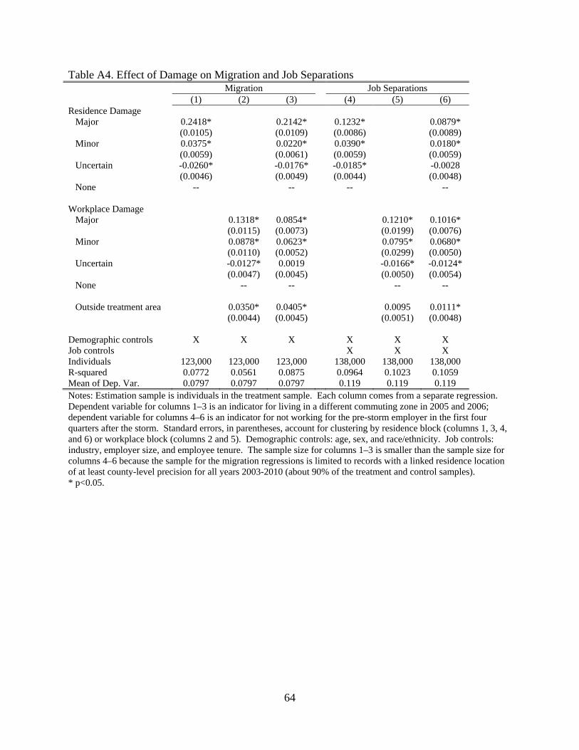
64

Table A4. Effect of Damage on Migration and Job Separations Migration Job Separations (1) (2) (3) (4) (5) (6) Residence Damage Major 0.2418* 0.2142* 0.1232* 0.0879* (0.0105) (0.0109) (0.0086) (0.0089) Minor 0.0375* 0.0220* 0.0390* 0.0180* (0.0059) (0.0061) (0.0059) (0.0059) Uncertain -0.0260* -0.0176* -0.0185* -0.0028 (0.0046) (0.0049) (0.0044) (0.0048) None -- -- -- -- Workplace Damage Major 0.1318* 0.0854* 0.1210* 0.1016* (0.0115) (0.0073) (0.0199) (0.0076) Minor 0.0878* 0.0623* 0.0795* 0.0680* (0.0110) (0.0052) (0.0299) (0.0050) Uncertain -0.0127* 0.0019 -0.0166* -0.0124* (0.0047) (0.0045) (0.0050) (0.0054) None -- -- -- -- Outside treatment area 0.0350* 0.0405* 0.0095 0.0111* (0.0044) (0.0045) (0.0051) (0.0048) Demographic controls X X X X X X Job controls X X X Individuals 123,000 123,000 123,000 138,000 138,000 138,000 R-squared 0.0772 0.0561 0.0875 0.0964 0.1023 0.1059 Mean of Dep. Var. 0.0797 0.0797 0.0797 0.119 0.119 0.119 Notes: Estimation sample is individuals in the treatment sample. Each column comes from a separate regression. Dependent variable for columns 1–3 is an indicator for living in a different commuting zone in 2005 and 2006; dependent variable for columns 4–6 is an indicator for not working for the pre-storm employer in the first four quarters after the storm. Standard errors, in parentheses, account for clustering by residence block (columns 1, 3, 4, and 6) or workplace block (columns 2 and 5). Demographic controls: age, sex, and race/ethnicity. Job controls: industry, employer size, and employee tenure. The sample size for columns 1–3 is smaller than the sample size for columns 4–6 because the sample for the migration regressions is limited to records with a linked residence location of at least county-level precision for all years 2003-2010 (about 90% of the treatment and control samples). * p<0.05.

65

Table A5. Distribution of Treatment and Control Samples across Industries Treatment Control Industry 2005:2 2006:2 2008:2 2012:2 2005:2 2006:2 2008:2 2012:2 Agriculture and resources 2.97 2.51 2.58 2.27 1.81 1.58 1.57 1.41 Construction 6.78 5.53 5.31 4.47 5.96 4.93 4.44 3.27 Manufacturing 12.70 10.98 10.59 8.94 13.84 12.39 11.04 8.92 Leisure, Accommodations 7.52 4.69 4.57 4.19 6.18 4.59 4.22 3.61 Healthcare 14.45 11.58 11.42 10.94 13.77 12.07 11.55 10.81 Professional services 12.73 10.48 10.37 9.41 14.15 12.63 11.87 10.42 Local services 17.00 13.22 12.57 10.96 17.39 13.87 12.85 11.45 Trade, Transport, Utilities 9.63 7.91 7.99 7.17 10.62 9.42 8.96 7.87 Public, Education 16.22 13.38 13.00 12.19 16.28 14.62 14.58 12.93 Not employed 19.72 21.62 29.46 13.90 18.92 29.31 Difference (Treatment - Control) Industry 2005:2 2006:2 2008:2 2012:2 Agriculture and resources 1.16 0.93 1.01 0.86 Construction 0.82 0.60 0.87 1.20 Manufacturing -1.14 -1.41 -0.45 0.02 Leisure, Accommodations 1.34 0.10 0.35 0.58 Healthcare 0.68 -0.49 -0.13 0.13 Professional services -1.42 -2.15 -1.50 -1.01 Local services -0.39 -0.65 -0.28 -0.49 Trade, Transport, Utilities -0.99 -1.51 -0.97 -0.70 Public, Education -0.06 -1.24 -1.58 -0.74 Not employed 5.82 2.70 0.15 Notes: Columns in the upper panel provide the distribution (in percentages) across industry sectors of the treatment and matched control samples at the beginning of each quarter listed. Industry assignments are for the highest-earning job in that quarter, among those held in the listed quarter and in the following quarter (referred to in QWI as an end-of-quarter job). The lower panel provides differences between the industry distributions of the treatment and matched control samples in each quarter.

66

Table A6. Effects on Earnings by Subgroup based on Pre-Storm Attachment to Employment Pre-storm Effects by Time Period after the Storm Dimension Category Pct. earnings Short Medium Long Full

All 100 9,916 -298.4 343.0* 792.3* 403.8* (191.4) (125.4) (141.8) (127.9) [-3.0] [3.5] [8.0] [4.1]

Employed in Yes 78.2 10,640 -358.1 316.9* 753.1* 371.4* all 8 pre-storm (208.2) (142.5) (153.8) (146.5) quarters [-3.4] [3.0] [7.1] [3.5]

No 21.8 7,322 -81.5 435.2* 926.5* 517.9* (148.9) (103.5) (152.7) (97.5) [-1.1] [5.9] [12.7] [7.1]

Same employer Yes 62.2 10,935 -377.1 289.2 773.9* 366.5* in all 8 pre- (219.5) (149.9) (140.6) (147.4) storm quarters [-3.4] [2.6] [7.1] [3.4]

No 37.8 8,237 -169.4 433.8* 829.3* 468.2* (152.9) (111.5) (168.2) (117.3) [-2.1] [5.3] [10.1] [5.7]

Combination Employed all 8 and 62.2 10,935 -377.1 289.2 773.9* 366.5* of employed same employer (219.5) (149.9) (140.6) (147.4) and tenure [-3.4] [2.6] [7.1] [3.4]

Employed all 8 and 16.0 9,487 -282.8 438.0* 704.9* 406.8* different employer (173.8) (152.5) (243.0) (168.9) [-3.0] [4.6] [7.4] [4.3] Not employed all 8 21.8 7,322 -81.5 435.2* 926.5* 517.9* (148.9) (103.5) (152.7) (97.5) [-1.1] [5.9] [12.7] [7.1]

Notes: The estimates in each row are based on a separate regression. Numbers in column labeled “Pct.” are the percent of the treatment sample in each group. Standard errors are in parentheses. Pre-storm earnings are average earnings in 2005:2 for the treatment sample. Numbers in brackets are effects as a percent of average pre-storm earnings for each group. Short term is 2005:4–2006:3 (k=1–4), medium term is 2007:4–2008:3 (k=9–12), long term is 2011:4–2012:3 (k=25–28), and full is 2005:4–2012:3 (k=1–28). * p<0.05.

67

Table A7. Effects on Earnings by Subgroup based on Demographic Characteristics Pre-storm Effects by Time Period after the Storm Dimension Category earnings Short Medium Long Full

All 9,916 -298.4 343.0* 792.3* 403.8* (191.4) (125.4) (141.8) (127.9) [-3.0] [3.5] [8.0] [4.1]

Education Less than high school 6,848 -54.1 682.1* 969.0* 652.6* (146.9) (103.5) (121.6) (102.3) [-0.8] [10.0] [14.2] [9.5]

High school 8,274 13.6 586.3* 809.0* 589.9* (124.7) (87.6) (111.7) (89.4) [0.2] [7.1] [9.8] [7.1]

Some college 9,462 -192.8 341.3* 714.6* 405.8* (148.4) (105.4) (98.6) (97.9) [-2.0] [3.6] [7.6] [4.3]

College 14,676 -910.1* -70.9 915.4* 127.3 (411.5) (324.2) (447.7) (344.4) [-6.2] [-0.5] [6.2] [0.9]

Age in 25 ≤ Age < 30 7,352 12.4 98.0 588.6 249.0 2005 (138.7) (174.2) (432.1) (224.7)

[0.2] [1.3] [8.0] [3.4] 30 ≤ Age < 40 9,304 -326.7 430.3* 776.3* 449.8*

(211.8) (159.8) (210.8) (172.1) [-3.5] [4.6] [8.3] [4.8]

40 ≤ Age < 50 10,558 -394.7 410.6* 855.7* 439.8* (206.0) (123.9) (133.5) (122.2) [-3.7] [3.9] [8.1] [4.2]

50 ≤ Age < 60 11,144 -292.8 275.1 841.3* 384.2* (215.6) (146.6) (188.1) (133.0) [-2.6] [2.5] [7.6] [3.4]

Sex Female 7,417 -410.8* 56.2 290.9* 92.5 (200.4) (108.5) (77.4) (98.4) [-5.5] [0.8] [3.9] [1.2]

Male 12,409 -194.8 625.6* 1,299.0* 715.5* (208.2) (178.9) (235.3) (185.0) [-1.6] [5.0] [10.5] [5.8]

Race/ White, not Hispanic 11,135 -244.8 399.2* 951.7* 489.3* Ethnicity (180.9) (146.2) (180.4) (145.5)

[-2.2] [3.6] [8.5] [4.4] Black, not Hispanic 7,099 -481.1 204.7 428.3* 188.4

(312.4) (143.8) (130.7) (151.6) [-6.8] [2.9] [6.0] [2.7]

Hispanic + Other race/NH 9,627 -106.0 363.6 738.6* 446.5* (176.9) (199.2) (289.3) (178.0) [-1.1] [3.8] [7.7] [4.6]

Notes: The estimates in each row are based on a separate regression. Pre-storm earnings are average earnings in 2005:2 for the treatment sample. Numbers in parentheses are standard errors clustered at the county level (based on 2005 residence location). Numbers in brackets are effects as a percent of average pre-storm earnings for each group. Short term is 2005:4–2006:3 (k=1–4), medium term is 2007:4–2008:3 (k=9–12), long term is 2011:4–2012:3 (k=25–28), and full is 2005:4–2012:3 (k=1–28). * p<0.05.

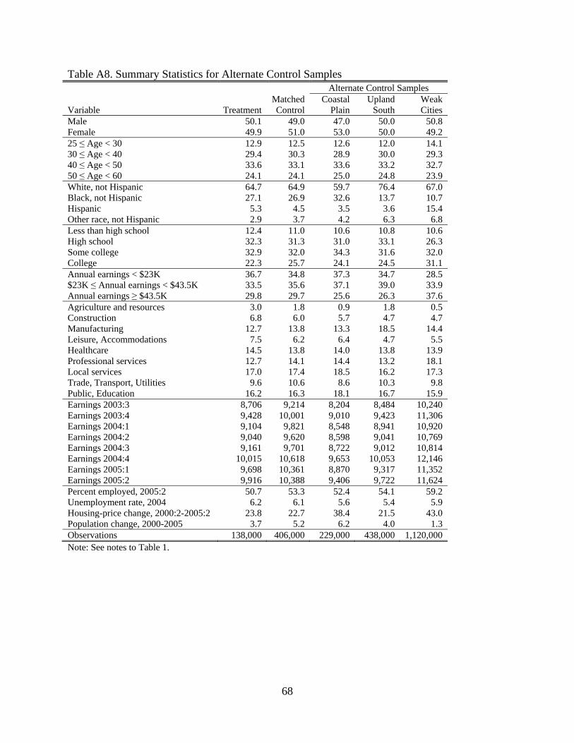
68

Table A8. Summary Statistics for Alternate Control Samples Alternate Control Samples

Variable Treatment Matched Control

Coastal Plain

Upland South

Weak Cities

Male 50.1 49.0 47.0 50.0 50.8 Female 49.9 51.0 53.0 50.0 49.2 25 ≤ Age < 30 12.9 12.5 12.6 12.0 14.1 30 ≤ Age < 40 29.4 30.3 28.9 30.0 29.3 40 ≤ Age < 50 33.6 33.1 33.6 33.2 32.7 50 ≤ Age < 60 24.1 24.1 25.0 24.8 23.9 White, not Hispanic 64.7 64.9 59.7 76.4 67.0 Black, not Hispanic 27.1 26.9 32.6 13.7 10.7 Hispanic 5.3 4.5 3.5 3.6 15.4 Other race, not Hispanic 2.9 3.7 4.2 6.3 6.8 Less than high school 12.4 11.0 10.6 10.8 10.6 High school 32.3 31.3 31.0 33.1 26.3 Some college 32.9 32.0 34.3 31.6 32.0 College 22.3 25.7 24.1 24.5 31.1 Annual earnings < $23K 36.7 34.8 37.3 34.7 28.5 $23K ≤ Annual earnings < $43.5K 33.5 35.6 37.1 39.0 33.9 Annual earnings ≥ $43.5K 29.8 29.7 25.6 26.3 37.6 Agriculture and resources 3.0 1.8 0.9 1.8 0.5 Construction 6.8 6.0 5.7 4.7 4.7 Manufacturing 12.7 13.8 13.3 18.5 14.4 Leisure, Accommodations 7.5 6.2 6.4 4.7 5.5 Healthcare 14.5 13.8 14.0 13.8 13.9 Professional services 12.7 14.1 14.4 13.2 18.1 Local services 17.0 17.4 18.5 16.2 17.3 Trade, Transport, Utilities 9.6 10.6 8.6 10.3 9.8 Public, Education 16.2 16.3 18.1 16.7 15.9 Earnings 2003:3 8,706 9,214 8,204 8,484 10,240 Earnings 2003:4 9,428 10,001 9,010 9,423 11,306 Earnings 2004:1 9,104 9,821 8,548 8,941 10,920 Earnings 2004:2 9,040 9,620 8,598 9,041 10,769 Earnings 2004:3 9,161 9,701 8,722 9,012 10,814 Earnings 2004:4 10,015 10,618 9,653 10,053 12,146 Earnings 2005:1 9,698 10,361 8,870 9,317 11,352 Earnings 2005:2 9,916 10,388 9,406 9,722 11,624 Percent employed, 2005:2 50.7 53.3 52.4 54.1 59.2 Unemployment rate, 2004 6.2 6.1 5.6 5.4 5.9 Housing-price change, 2000:2-2005:2 23.8 22.7 38.4 21.5 43.0 Population change, 2000-2005 3.7 5.2 6.2 4.0 1.3 Observations 138,000 406,000 229,000 438,000 1,120,000 Note: See notes to Table 1.

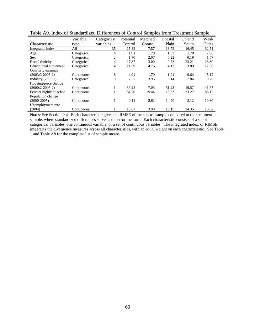
69

Table A9. Index of Standardized Differences of Control Samples from Treatment Sample

Characteristic Variable type

Categories/ variables

Potential Control

Matched Control

Coastal Plain

Upland South

Weak Cities

Integrated index All 35 25.82 7.57 18.72 16.45 32.51Age Categorical 4 1.91 1.20 1.33 1.78 2.06Sex Categorical 2 1.70 2.07 6.22 0.19 1.57Race/ethnicity Categorical 4 27.87 3.00 9.73 23.21 28.80Educational attainment Categorical 4 11.39 4.76 4.12 3.89 12.36Quarterly earnings (2003:3-2005:2) Continuous 8 4.94 1.70 1.91 0.64 5.12Industry (2005:3) Categorical 9 7.25 3.95 6.14 7.84 9.26Housing-price change (2000:2-2005:2) Continuous 1 35.25 7.05 51.23 19.57 41.57Percent highly attached Continuous 1 64.70 19.44 15.33 33.27 85.12Population change (2000-2005) Continuous 1 0.11 8.62 14.90 2.12 19.80Unemployment rate (2004) Continuous 1 15.67 3.90 15.15 24.35 10.02Notes: See Section 9.4. Each characteristic gives the RMSE of the control sample compared to the treatment sample, where standardized differences serve as the error measure. Each characteristic consists of a set of categorical variables, one continuous variable, or a set of continuous variables. The integrated index, or RIMSE, integrates the divergence measures across all characteristics, with an equal weight on each characteristic. See Table 1 and Table A8 for the complete list of sample means.

70

Figure A1. County-Level Damage

Source: FEMA damage data provided by HUD (2006). Notes: Legend shows the share of housing units in a county with damage in excess of $5,200. The map shows 122 counties in Texas, Louisiana, Mississippi, and Alabama. Hurricane Katrina made landfall in the east and Hurricane Rita made landfall in the west.

Texas Louisiana

Mississippi Alabama

40 - 10010 - 405 - 101 - 50 - 1

71

Figure A2. Treatment Counties, County Damage Level, and Sub-County Damage Data

Notes: Figure breaks down the 63 treatment counties into three types. The 41 counties shown in white have at least 1 percent of housing units with damage in excess of $5,200 (HUD, 2006) but do not have sub-county damage data (FEMA, 2005). The 19 counties shown in dark gray have at least 1 percent of housing units with damage in excess of $5,200 and have sub-county damage data. The 3 counties shown in light gray have less than 1 percent of housing units with damage in excess of $5,200 but have sub-county damage data.

Texas Louisiana

Mississippi Alabama

72

Figure A3. Major and Minor Damage Panel A. New Orleans, Louisiana (and surrounding areas)

Panel B. Gulf Coast of Mississippi

Source: Damage information from FEMA (2005). Notes: Panels A and B depict damage from Hurricane Katrina, along with county names and boundaries. Red indicates major damage, dark blue indicates minor damage, green indicates undamaged land area, and light blue indicates bodies of water. Both maps are to the same scale and depict an area approximately 40 miles wide.

Orleans

Jefferson

St. Bernard

St. Charles

Plaquemines

HarrisonHancock

Jackson

73

Figure A4. Major and Minor Damage Overlaid with Census Blocks Panel A. Orleans Parish, Louisiana

Panel B. Harrison County, Mississippi

Source: Damage information from FEMA (2005). Notes: Panels A and B depict damage from Hurricane Katrina, along with boundaries of Census blocks. Red indicates major damage, dark blue indicates minor damage, green indicates undamaged land area, and light blue indicates bodies of water. Both maps are to the same scale and depict an area approximately 5.5 miles wide.

74

Figure A5. Average Earnings in Treatment and Control Samples

Note: See Figure 3 for description of earnings data. Figure A6. Alternate Control Areas

Notes: Map depicts the residence location of workers in alternate control samples. The Atlantic Coast (darker shading) control is in Florida, Georgia, South Carolina, North Carolina, and Virginia. The Upland South (lighter shading) control is in Oklahoma, Arkansas, and Tennessee. The Weak Cities (lighter shading) control is in California, Missouri, Illinois, Wisconsin, Indiana, Michigan, Ohio, Kentucky, West Virginia, Pennsylvania, Maryland, New Jersey, and New York.

Treatment

Control

8,500

9,000

9,500

10,000

10,500

11,000

-8 -6 -4 -2 0 2 4 6 8 10 12 14 16 18 20 22 24 26 28Quarters relative to storm

Atlantic Coast

Upland South

Weak Cities

75

Figure A7. Effects on Earnings with Alternate Control Samples

Notes: See Figure 3 for description of earnings data. Equation (1) provides the model specification. The sample for this analysis is the treatment sample paired with the either the matched, Coastal Plain, Upland South, or Weak Cities control sample. See Table A8 for sample sizes.

-500

0

500

1,000

1,500

-8 -6 -4 -2 0 2 4 6 8 10 12 14 16 18 20 22 24 26 28Quarters relative to storm

MatchedCoastalUpland

Weak