BLOWING RATIO EFFECTS ON FILM COOLING...

BLOWING RATIO EFFECTS ON FILM COOLING EFFECTIVENESS

A Thesis

by

KUO-CHUN LIU

Submitted to the Office of Graduate Studies ofTexas A&M University

in partial fulfillment of the requirements for the degree of

MASTER OF SCIENCE

August 2009

Major Subject: Mechanical Engineering

BLOWING RATIO EFFECTS ON FILM COOLING EFFECTIVENESS

A Thesis

by

KUO-CHUN LIU

Submitted to the Office of Graduate Studies ofTexas A&M University

in partial fulfillment of the requirements for the degree of

MASTER OF SCIENCE

Approved by:

Chair of Committee, J.C. HanCommittee Members, S.B. Wen

H.C. ChenHead of Department, Dennis O’Neal

August 2009

Major Subject: Mechanical Engineering

iii

ABSTRACT

Blowing Ratio Effects on Film Cooling Effectiveness. (August 2009)

Kuo-Chun Liu, B.S., Kansas State University

Chair of Advisory Committee: Dr. Je-Chin Han

The research focuses on testing the film cooling effectiveness on a gas turbine

blade suction side surface. The test is performed on a five bladed cascade with a

blow down facility. Four different blowing ratios are used in this study, which are

0.5, 1.0, 1.6, and 2.0; mainstream flow conditions are maintained at exit Mach

number of 0.7, 1.1 and 1.3. Nitrogen is injected as the coolant so that the oxygen

concentration levels can be obtained for the test surface. Based on mass transfer

analogy, film cooling effectiveness can be computed with pressure sensitive paint

(PSP) technique. The effect of blowing ratio on film cooling effectiveness is

presented for each testing condition. The spanwise averaged effectiveness for

each case is also presented to compare the blowing ratio and mainstream effect on

film cooling effectiveness. Results show that due to effects of shock, the optimum

blowing ratio is 1.6 for exit Mach number of 1.1 and 1.3; however; without the

effects of shock, the optimum blowing ratio is 1.0 for exit Mach number of 0.7.

iv

DEDICATION

To my parents and sister for their endless love, support and encouragement

v

ACKNOWLEDGEMENTS

I am very grateful to Dr. Je-Chin Han for mentoring me throughout my academic

work here at Texas A&M University. He has provided me with invaluable

experience as a research assistant in gas turbine studies. I am appreciative of Dr.

Sy-Bor Wen and Dr. Hamn-Ching Chen for serving on my committee and offering

valuable suggestions to improve my research and reports. I also thank my

partners, Michael Hue and Diganta Narzary, who spent lots of time and effort on

test section design, assembly and conducting the experiment.

vi

TABLE OF CONTENTS

Page

ABSTRACT..................................................................................................................... iii

DEDICATION ..................................................................................................................iv

ACKNOWLEDGEMENTS ...............................................................................................v

TABLE OF CONTENTS..................................................................................................vi

LIST OF FIGURES........................................................................................................ viii

LIST OF TABLES ......................................................................................................... xiii

NOMENCLATURE........................................................................................................xiv

INTRODUCTION AND LITERATURE REVIEW..........................................................1

Injection Hole Shape ......................................................................................................4Effects of Blowing Ratios ..............................................................................................5Free-Stream Turbulence Effects ....................................................................................7Effects of Density Ratios ...............................................................................................9Effects of Tip Leakage .................................................................................................10

OBJECTIVES ..................................................................................................................12

INSTRUMENTATION....................................................................................................13

DATA REDUCTION.......................................................................................................19

Pressure Sensitive Paint Technique .............................................................................20Film Cooling Effectiveness..........................................................................................22Blowing Ratio ..............................................................................................................24

RESULTS AND DISCUSSIONS ...................................................................................25

Mach Number Distribution ..........................................................................................25Film Cooling Effectiveness..........................................................................................29Overall Comprarison ....................................................................................................51

CONCLUSIONS..............................................................................................................56

vii

Page

REFERENCES.................................................................................................................57

VITA ................................................................................................................................60

viii

LIST OF FIGURES

Page

Figure 1. Blade cooling techniques ....................................................................................2

Figure 2. Compound angle and different shaped hole ...................................................... 3

Figure 3. Schematic of blow down facility and digital controller setup ......................... 14

Figure 4. Test section cascade assembly......................................................................... 15

Figure 5. Schematic of experimental facility .................................................................. 16

Figure 6. Drawing of test vane (a) suction side, (b) pressure side .................................. 17

Figure 7. Three temperature model for film cooling effectiveness................................. 19

Figure 8. A basic PSP setup ............................................................................................ 20

Figure 9. PSP calibration setup ....................................................................................... 21

Figure 10. Calibration curve used for the PSP method ................................................... 22

Figure 11. Mach number distribution contour plots for blowing ratio = 0 and exitMach numbers of (a) 0.7, (b)1.1, and (c) 1.3..................................................26

Figure 12. Mach number distribution contour plots for blowing ratio = 0.5 and exitMach numbers of (a) 0.7, (b)1.1, and (c) 1.3..................................................26




Figure 16. (a) Actual camera view for the test vane surface, and (b) Shaded area isthe field of camera view .................................................................................30

Figure 17. Cooling effectiveness distribution contour plots for blowing ratio = 0.5and exit mach numbers of (a) 0.7, (b)1.1, and (c) 1.3 ....................................31

ix

Page

Figure 18. Cooling effectiveness distribution contour plots for blowing ratio = 1.0and exit Mach numbers of (a) 0.7, (b)1.1, and (c) 1.3....................................31



Figure 21. Yellow-square area is the magnified region ...................................................33

Figure 22. Magnified Mach number and effectiveness distribution for exit Machnumbers of 1.1 and blowing ratio = 0.5 .........................................................34








Figure 30. a) 2D effectiveness distribution along surface length for and exit Machnumbers of 0.7 and blowing ratio = 0.5, b) corresponding span positionon the test vane surface ..................................................................................39


x

Page











Figure 42. Effectiveness along two spans position for and exit Mach numbers of0.7 and blowing ratio = 0.5 ............................................................................45

xi

Page







Figure 49. Effectiveness along two spans position for and exit Mach numbers of1.1and blowing ratio = 2.0 .............................................................................48





Figure 54. Effectiveness comparison of exit Mach number = 0.7 to 1.3 andblowing ratio = 0.5 and 1.0 ............................................................................52

Figure 55. Effectiveness comparison of exit Mach number = 0.7 to 1.3 andblowing ratio = 1.6 and 2.0 ............................................................................53

Figure 56. Spanwise averaged effectiveness comparison of blowing ratio = 0.5 ............54



xii

Page


xiii

LIST OF TABLES

Page

Table 1. Summary of experimental conditions ................................................................18

xiv

NOMENCLATURE

A total film cooling hole area, (m2)

hA single film cooling hole area, (m2)

C oxygen concentration of mainstream

mixC oxygen concentration of mainstream-coolant mixture

2NC oxygen concentration of nitrogen

DR density ratio

I momentum ratio

PI emission intensity of PSP

refPI emission intensity of PSP at reference (atmospheric) pressure

blackPI emission intensity of PSP at no-flow and without light excitation

M blowing ratio

m mass flow rate, (kg/s)

n number of film cooling holes

airOP 2 partial oxygen pressure in air, (Pa)

mixOP 2 partial oxygen pressure in coolant-air mixture, (Pa)

T temperature, (K)

cT coolant temperature, (K)

T mainstream temperature, (K)

cV average coolant velocity, (m/s)

xv

mV mainstream velocity, (m/s)

cQ volumetric flow rate of coolant, (m3/s)

specific heat ratio

film cooling effectiveness

c coolant density, (kg/m3)

m mainstream density, (kg/m3)

1

INTRODUCTION AND LITERATURE REVIEW

The gas turbine industry engineers are always trying to increase the turbine inlet

temperature due to its significant promotion to thrust and thermal efficiency. However,

a high inlet temperature will induce some major problems to the turbine blade. For

example, the design operating temperature of turbine is above melting temperature of the

material; therefore, the blade is not able to withstand such high temperatures and thermal

stresses. In modern gas turbine technology, numerous cooling techniques have been

developed to prevent the blade and vane from damage. Han et al. [1] describes many

cooling techniques that are commonly used in various combinations to increase the

lifetime of the turbine blade. Internal cooling method, including impingement cooling,

rib-turbulated cooling, and pin-fin cooling, is used to remove heat from the inside of the

blade. Figure 1 shows the typical cooling methods of modern gas turbine blades.

External cooling method is mostly focused on film cooling technique, in which cool air

is bled from the compressor stage, ducted to the internal chambers of the turbine blades,

and discharged through small holes in the blade walls into the hot mainstream. The

discharged coolant air provides a thin, relatively cool layer on the outer surface of the

blade and functions as an insulator. After all, the blade is able to withstand the

extremely hot mainstream gases and has a longer lifetime cycle.

____________This thesis follows the style of ASME Journal of TurboMachinery.

2

Fig. 1 Blade cooling techniques

Film cooling technique is facing two major issues: (1) when we supply too much coolant

into the film cooling chamber, instead of forming a thin layer and attaching on the blade

surface, it will penetrate into the mainstream. Thus, the blade losses the protection and

has no cooling effectiveness, and (2) the space between two discrete cooling holes is not

covered well by the coolant layer. Above situations causes hot spots on the blade

surface and results a non-uniform cooling distribution.

Engineers are always trying to maximize the cooling efficiency by using less coolant and

have optimum cooling results. Designers and researchers discovered that injection hole

geometry has a significant effect on cooling efficiency.

Dovetail

TrailingEdgeSlots

Film coolingholes

Tip capholes

Squealer tip

Bladeplatform

Coolingair

Jetimpingementcooling

Ribturbulatedcooling

Impingementcooling

Hotgas

Film cooling

Ribturbulators Shaped internal

cooling passage

Trailingedgeejection

Coolingair

3

Among the variety of film cooling hole designs, compound angle and shaped holes are

generally considered in modern high pressure and high temperature gas turbine engines.

Figure 2 shows the schematic hole geometries and the cross section view cutting along

the hole centerline. The compound angle hole provides better effectiveness as the

coolant is deflected by the mainstream and covers a wider area. The shaped hole

performs better because the expanded diffused area reduces the jet momentum and

prevents the coolant separate from the blade surface.

Fig. 2 Compound angle and different shaped hole

4

Injection Hole Shape

There are many experimental studies focusing on different hole configurations and

geometries. Goldstein et al. [2] were the first to investigate the shaped injection holes to

improve film cooling performance. They compared the film cooling effectiveness for

cylindrical holes and axial fanshaped hole with lateral diffusion of 10 º. They determined

a significant improvement of film cooling effectiveness and coolant coverage of the

shaped hole.

Sen et al. [3] and Schmidt et al. [4] studied forward diffused holes. They discovered that

the 15ºforward diffused holes also provide better effectiveness than cylindrical holes.

Thole et al. [5] measured the flow fields for three types of injection holes: a cylindrical

hole, a laterally diffused hole, and a forward-laterally diffused hole. Their results

showed that diffusing the injection hole reduces the coolant penetration into the

mainstream and reduces the intense shear regions when compared to cylindrical holes.

Gritsch et al. [6] studied the same cooling hole configuration and orientation as [5] with

a density ratio of 1.85. As compared to cylindrical hole, both shaped holes showed

significant improved thermal protection of the surface downstream of the ejection

location.

Yu et al. [7] studied film cooling effectiveness and heat transfer distributions on a flat

plate with cylindrical hole, laidback hole, and laidback shaped hole. The laidback

5

shaped hole provided the highest film cooling effectiveness and overall heat transfer

reduction.

In 2007, Gao et al. [8] studied the film effectiveness laidback fanshape hole geometries

with compound angles using the PSP technique. The coolant is only injected to either

pressure side or suction side of the blade. Upstream wake simulation is done by placing

a periodic set of rod upstream of the test blade. The free stream Reynolds number, based

on the axial chord length and the exit velocity, is 750,000 and the inlet and exit Mach

numbers are 0.27 and 0.44. They investigated that laidback fanshape holes with

compound angle provide very good coolant t film coverage on the suction side. Overall,

the compound angle shaped holes perform the much better than compound angle

cylindrical holes by expanding diffused area.

Effects of Blowing Ratios

Blowing ratio is defined as mass flux ratio between coolant and mainstream. This has

been extensively studied to maximize the film cooling effectiveness. Optimizing the

blowing ratio is important, because low blowing ratio would not provide enough coolant

to cover the blade surface effectively; however, blowing ratio is too high causes the

coolant shoot into the mainstream. Studies have also shown the optimum blowing ratios

are not the same for every hole shape.

6

Goldstein et al. [2, 9] showed cylindrical holes have the optimum blowing ratio abound

M = 0.5. The higher blowing ratios cause coolant jets penetrated into the mainstream

and reduce the cooling effectiveness. Further downstream the effectiveness tended to

increase with the blowing rate where the coolant jets reattached to the surface.

Cho et al. [10] compared the blowing ratio effects for two different types of hole shapes.

(1) diffused 4 ºin all direction, (2) forward diffusion of 8 º. As blowing ration increases,

the coolant becomes more separate from the surface and reduces the cooling

effectiveness. The optimum blowing ratio for cylindrical hole in this study is closed to

M = 0.5. Shaped hole #1 also showed decreasing effectiveness for increasing blowing

ratios. However, film cooling effectiveness values did not drop till M = 1.0. Shaped

hole #2 performed similarly when compared to the other holes. At the highest blowing

ratio of M = 2.0, the effectiveness distribution was more similar to the cylindrical hole

rather than the shaped hole #1. Because this hole has an expansion in the forward

direction only, the diffusion of coolant in the hole is not uniform. Therefore the

interaction between the mainstream and the coolant is stronger.

Gao et al. [8] studied film cooling effectiveness distribution on the blade pressure side or

suction side with axial hole without showerhead film cooling. Their results showed the

moderate blowing ratios M = 0.6 to 1.2 gave better film cooling effectiveness. Further

increasing blowing ratio to M = 1.5, the effectiveness decreases because coolant jet

liftoff.

7

Free-Stream Turbulence Effects

Turbulence is generated by using grids upstream of the test section, the grid functions as

a blockage to the flow. Jet grids are also used to generate free stream turbulence. Air is

forced through an array of pipes into mainstream. At the exit of combustor, the

turbulence intensity is about 7 to 20%; thus, the first stage vane can have the turbulent

inlet boundary condition as high as 20%.

Saumweber et al. [11] found that the free stream turbulence in tensity is reduced because

of air accelerates through the vane. Free-stream turbulence levels at engine conditions

can therefore be in the range of 8 to 12%.

Kadotani and Goldstein [12, 13] tested turbulent intensities ranging form 0.3 to 20.6%

with length scales between 0.06 and 0.33 cylindrical holes inclined 33ºto the

mainstream. At low blowing ratio, high turbulent intensities produced a decrease in

centerline effectiveness. At high blowing ratio, however, high turbulence increased the

centerline effectiveness. This was because the turbulent mixing reduced the penetration

of the coolant into the mainstream. Additionally, the high turbulence improved the

lateral distribution of the coolant for the cylindrical holes. Low turbulence, however,

creates a more uniform lateral distribution of effectiveness.

Mehendal and Han [14] studied the high turbulence intensity effect on the turbine blade

leading edge. They measured the cooling effectiveness on the semicircular leading edge

8

with flat downstream body by using thermal couples. The blowing ratio was varied from

0.4 to 1.2 for different free stream turbulence levels. High turbulence intensity was

generated by passive grid (9.67%) and jet grid (12.9%). They found that the free stream

turbulence reduces the film cooling effectiveness at blowing ratio of 0.4. Higher free

stream turbulence intensity causes coolant jet to dissipate into the mainstream faster.

Beside, the unsteady mainstream penetrates and mixes with film cooling layer and

reduces the effectiveness. The coolant jet attaches on the blade surface and maintained

over a long distance when turbulence intensity is low, and provides higher effectiveness.

By increasing the coolant ratio, the coolant jet momentum is stronger and unsteady

mainstream causes fewer disturbances. Therefore it has less turbulence effect on high

blowing ratio film cooling effectiveness.

Burd et al. [15] had an important founding that the L/D ratio of the film cooling hole has

to be taken into account when comparing turbulent intensity effects on film cooling.

They measured mainstream turbulence intensity by using hot wire anemometer on

cylindrical holes angled 35ºto the mainstream. Two turbulent intensities (0.5 and 12%)

while varying the L/D ratio from 2.3 to 7 had been tested. With low free-stream

turbulence and short holes, the coolant is ejected farther from the wall and spreads more

in the spanwise direction when compared to a long hole. At high free-stream turbulence,

though, the flow differences between a long and short hole greatly decrease

9

Gao et al. [16] took the measurement in a five-bladed linear cascade facility. They used

metal rods placed periodically upstream of the test blade to simulate the stationary,

upstream wake. The rods were placed upstream of the blades at the 50% axial chord

length. Rods locations for 0%, 25%, 50% and 75% were progressively located along the

blade pitch-wise direction. They concluded that the wake rod locations of 0% and 25%

significantly decrease the film cooling effectiveness; however, wakes from 50% and

75% locations may not attach to the blade surfaces and hence do not impact the film

cooling effectiveness as much.

Effects of Density Ratios

In real engines, the coolant to mainstream density ratio is close to 2. Because the

coolant is at lower temperature and higher pressure than the mainstream, which causes

the density difference. Rather than using nitrogen to be the coolant, which has similar

molecular weight as air, other gases have greater molecular weight are considered to be

used.

Pedersen et al. [17] investigated the effect of blowing ratio of film cooling effectiveness.

They tested various density ratios from 0.75 to 4.17. They found out as density ratio

increases, the peak on cooling effectiveness moves toward to higher blowing ratio. Thus,

they concluded that greater density ratio coolant tends to attach closer to the blade

surface compared to the light density ratio coolant at the same blowing ratio.

10

Sinha et al. [18] studied similarly on various density ratio coolants under different

blowing ratio. For a constant density ratio, the film cooling effectiveness reaches a peak

as blowing ratio increases and starts to drop off at very high blowing ratio. This is

because the coolant ejection penetrates through the mainstream and losses the protection

of the blade surface. Peaks move toward higher blowing ratio by increasing density ratio

and provide higher effectiveness. Because of less mixing and lower momentum, the

higher density coolants stay closer to the surface. They also shows the film effectiveness

with momentum flux ratio, since momentum flux ratio is the combination of blowing

ratio and density ratio, it scales the better effects on film effectiveness.

Effects of Tip Leakage

In most experimental studies, blade film cooling is focused on the mid-span region only;

the effects of endwall and tip leakage were not captured. Mhetras and Han [19] obtained

detailed film cooling effectiveness distribution on a fully film cooled blade surface by

using PSP technique. There are three showerhead rows of cylindrical holes with an

angle of 30 in radial direction in the leading region. There were compound angle holes

on the blade surface, four rows on the pressure side and two rows on the suction sides.

During the test, all holes are opened. They showed that the coolant on the suction side

was swept toward the mid-span region due to tip leakage vortices and endwall vortices.

Blowing ratios are varied from M = 0.3 to M = 1.2, results showed the compound angle

cylindrical hole obtained highest cooling effectiveness at M = 0.9. In another paper,

Mhetras and Han [20], they studied the upstream film cooling accumulation effect on the

11

downstream film cooling using superposition method. Four rows and two rows of

compound angle cylindrical holes were arranged on the pressure and suction sides.

Results showed the film cooling effectiveness on the suction side is much higher than

the pressure side. Superposition from individual cooling rows shows good agreement

with experimental data.

12

OBJECTIVES

The research focuses on testing the film cooling effectiveness on a gas turbine blade

suction side surface for different blowing ratios and mainstream velocities. Test is

performed on a five bladed cascade with a blow down facility. Based on mass transfer

analogy, film cooling effectiveness is measured with pressure sensitive paint (PSP)

technique. Test vane has three rows of cylindrical holes on the leading edge, and two

rows of compound angle shaped holes on the suction side. Each row has total 7 film

cooing holes. Four different blowing ratios are used in this study, which are 0.5, 1.6, 2.0

and 3.0. Experiment is operated under three mainstream flow conditions, one is with

subsonic exit velocity as Mach number = 0.7 and the others are with supersonic exit

velocities as Mach number = 1.1 and 1.3.

13

INSTRUMENTATION

The experiment is tested in the test section consisted of a stationary blow-down facility

with a five-bladed annular cascade. Figure 3 shows the schematic setup of blow down

facility and digital controllers. Compressed air store in the tanks entered a high flow

pneumatic control valve that was designed to receive feedback from the downstream

pressure to mainstream a velocity within ±3% of the desired value. The inlet and exit

transition dusts of the test section had inner diameter of 4 inch and were made of 0.125

inch thick aluminum.

As shown in Figure 4, the cascade was made of Selective Laser Sintering (SLS). A

viewing window was made of transparent Stereolithograpgy (SLA) and was installed

above the test vane, a SLS strip was attached with the window in order to provide

additional reinforcement. In the cooling effectiveness test, a 12-bit, scientific grade

CCD camera (Cooke Sensicam QE with CCD temperature maintained at -15°C using 2-

stage peltier cooler) and a strobe light (PerkinElmer MVS-7000 Series) fitted with a

narrow band-pass filter (optical wavelength = 520 nm) were placed above the viewing

window. A turbulence grid was installed upstream of the test section.

14

1.Inlet Transition Duct2.Annular Cascade3.Exit Transition Duct

1.Inlet Transition Duct2.Annular Cascade3.Exit Transition Duct

Fig. 3 Schematic of blow down facility and digital controller setup

Compressed Air

1. Inlet Transition Duct

2. Cascade

3. Exit Transition Duct

15

Fig. 4 Test section cascade assembly

Pitot tubes are placed at the inlet and the exit of the test section to measure the total and

static pressures. Coolant is ejected to leading edge (3 rows of cylindrical holes) and

suction side (2 rows of compound angle shaped holes); three ASME Orifice flow meters

are used to control the coolant volumetric flow rate and adjust the blowing ratios. Static

pressure taps are attached at the flow meter exit to measure the coolant pressure. The

entire experimental setup, including cascade, coolant supply and camera position are

shown is Figure 5.

16

Fig. 5 Schematic of experimental facility

During the blow down test, the cascade exit air velocities are maintained at Mach

number 0.7, 1.1 and 1.3, respectively. The corresponding Reynolds numbers based on

axial chord length and exit mainstream velocity are 6.33105, 9.98105 and 1.18106.

17

Test vane was made of SLS and its height decreases from the leading edge to trailing

edge as of 5.85 cm to 4.63 cm. The axial chord length of the blade is 3.96 cm. The

blade has 3 rows of cylindrical film cooling holes on leading edge, and 2 rows of

compound angle shaped holes on suction side surface. Each row has total 7 film cooling

holes as shown in Figure 6. Cylindrical holes have a 15.8° incline angle with respect to

vertical direction, and the compound angle shaped holes held an angle of 15.8° to the

axial direction. As shown in Table 1, the experiments are tested under blowing ratio of

0.5, 1.0, 1.6 and 2.0 with exit Mach number of 0.7, 1.1 and 1.3.

Fig. 6 Drawing of test vane (a) suction side, (b) pressure side

18

Table 1. Summary of experimental conditions

Expt. Exit Mach Number Blowing Ratio Coolant

1 0.7 0.5 N2

2 0.7 1.0 N2

3 0.7 1.6 N2

4 0.7 2.0 N2

5 1.1 0.5 N2

6 1.1 1.0 N2

7 1.1 1.6 N2

8 1.1 2.0 N2

9 1.3 0.5 N2

10 1.3 1.0 N2

11 1.3 1.6 N2

12 1.3 2.0 N2

19

DATA REDUCTION

The method used to calculate the film cooling effectiveness is called pressure sensitive

paint (PSP). An overview of the effectiveness measuring techniques is found in Han et

al. [1]. Film cooling involves the mainstream temperature ( mT ), the coolant temperature

( cT ), and the film temperature ( fT ). Figure 7 shows a diagram for the three

temperatures involved in film cooling. The efficiency of film cooling is quantified by a

parameter known as film cooling effectiveness, η. It is defined in Equation 1.

mc

mf

TT

TT

(1)

Fig. 7 Three temperature model for film cooling effectiveness

Mainstream Flow

X=0

q''=h(T - T )wm

mT , Vm

k

c cT , V

Tf

Mainstream Flow

X=0

q''=h(T - T )wm

mT , Vm

k

c cT , V

Tf

)("wm TThq

fT

cc VT ,

mm VT ,

wT

20

Pressure Sensitive Paint Technique

Data for film cooling effectiveness were measured using the PSP technique. Several

authors such as Han et al. [1], Zhang and Jaiswal [35], and Zhang and Fox [36] have

discussed this type of technology. A basic PSP setup is shown in Figure 8. PSP is

formed from a polymer binder with luminescent molecules suspended in the binder.

This binder is permeable, allowing oxygen molecules to penetrate into the paint, and

interact with the luminescent molecules. A light source excites the molecules, and when

the molecules return to their ground state, a longer wavelength luminescent light is

emitted through a process called fluorescence. The premise behind PSP is an oxygen

quenching effect. As the oxygen partial pressure of the gas in direct contact with the

surface increases, the intensity of the light emitted by the PSP decreases (hence, oxygen

quenched).

Fig. 8 A basic PSP setup

ExcitationSource with

Filter (520 nm)

CCD Camerawith Filter(>610 nm)


Filter (520 nm)




Filter (520 nm)

21

Calibration of PSP system was performed using a vacuum chamber at several known

pressure varying form 0 to 1 atm. A test plate is sprayed with the Uni-FIB PSP (UF470-

750) supplied by Innovative Scientific Solutions, Inc. (ISSI) and placed inside the

chamber as shown in Figure 9. At each measurement point, the PSP sample is excited

using a strobe light equipped with a 500 nm broadband pass filter. A 12-bit, scientific

grade CCD camera with a 630 nm filter records the intensity emitted by the PSP.

Test Sample Coated with PSP

Surface Temperature controlled by heater

VacuumChamber withOptical Access

CCDCamera

Excitation

Light

PC

Thermocouple Test Sample Coated with PSP

Surface Temperature controlled by heater

VacuumChamber withOptical Access

CCDCamera

Excitation

Light

PCPC

Thermocouple

Fig. 9 PSP calibration setup

A transparent window is located over the test surface, and the CCD camera is mounted

above the window. The strobe light is positioned so that maximum excitation of the PSP

occurs. The camera records the emitted intensity of the PSP as gray-scale images, which

are saved as TIFF files. The resulting intensity ratio can be converted to pressure ratio

using a pre-determined calibration curve and can be expressed as:

22

ratio

refO

airO

black

blackref PfP

Pf

II

II

2

2 (2)

It was observed that if the emitted light intensity at certain temperature was normalized

with the reference image intensity at the same temperature, the temperature sensitivity

can be minimized. Figure 10 shows the results of the calibration curve.

y = -0.3002x3 + 0.9034x2 + 0.3961x + 0.0059R2 = 0.9996

0

0.1

0.2

0.3

0.4

0.5

0.6

0.7

0.8

0.9

1

0.0 0.1 0.2 0.3 0.4 0.5 0.6 0.7 0.8 0.9 1.0

(Iref-Iblack)/(I-Iblack)

P/P

ref

Fig. 10 Calibration curve used for the PSP method

Film Cooling Effectiveness

Four images are needed to calculate the film effectiveness: a dark image (no light, no

mainstream), a reference image (with light, with mainstream), and an air injection image

(with light, with mainstream, coolant is air), and a nitrogen injection image (with light,

with mainstream, coolant is nitrogen). The air injection image contains information of

23

surface static pressure only, while the nitrogen injection image contains both the surface

static pressure and the oxygen concentration information. With the calibration curve, the

measured intensities are converted to the partial oxygen concentrations on the test

surface.

Based on mass transfer analogy, film cooling effectiveness equation can be rewritten in

terms of concentration of oxygen. Nitrogen which has nearly the same molecular weight

as air, by noting the difference in partial pressure between air and nitrogen injection

cases, the film cooling effectiveness can be determined using the following equation.

airO

mixOairOmix

N

mix

P

PP

CCC

CCCC

2

22

2

(3)

Here C is the oxygen concentration of the mainstream (near 21%) and mixC is the

oxygen concentration of the mainstream-coolant mixture (between 0 and 21 %). As a

result, the film effectiveness will be between 0% far downstream of the coolant injection

and 100% inside the hole. The mass fraction of the tracer gas in the mixture near the test

surface is related to the adiabatic wall temperature for the analogous heat transfer

situation.

24

Blowing Ratio

PSP technique is used to measure the mainstream pressure along the blade surface.

Pressure taps are installed at the flow meter exit portion to measure the coolant pressure;

mainstream and coolant densities can be calculated by applying ideal gas law. Blowing

ratio is computed based on coolant/mainstream density, mainstream velocity, coolant

volumetric flow rate and total film cooling hole area.

mm

h

cc

mm

c

mm

cc

VnA

Q

VAm

VV

M

(4)

25

RESULTS AND DISCUSSIONS

Mach Number Distribution

By taking images at no coolant (blowing ratio = 0), it provided the mainstream Mach

number distribution and static pressure on the test vane surface. As the exit mainstream

velocity become supersonic (Mach number = 1.1 and 1.3), shockwaves take place and

affect the film cooling effectiveness. Mach number distribution for three different exit

Mach numbers and blowing ratio = 0 are plotted in Figure 11. By distinguishing the

discontinuous velocity contour region, we can indicate the locations of potential

shockwave. Dotted lines represent the approximate cooling hole row location on the

suction side surface; the potential shock regions are pointed by arrows. In no coolant

case, it shows that for exit Mach number = 1.1 and 1.3, shockwaves take place at near-

to-trailing-edge region on the suction side surface of the test vane.

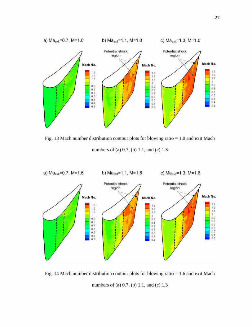
Similar Mach number distribution plots for blowing ratios of 0.5, 1.0, 1.6 and 2.0 are

shown in Figures 12 to 15. Results show that, with coolant ejection, shock locates at

almost the same locations for supersonic exit mainstream conditions. Due to ejected

coolant mixed with mainstream air and causes complex turbulence and mixing, Mach

number distribution and shockwaves’location are different than no coolant case (M = 0).

26

Fig. 11 Mach number distribution contour plots for blowing ratio = 0 and exit Mach

numbers of (a) 0.7, (b) 1.1, and (c) 1.3

Fig. 12 Mach number distribution contour plots for blowing ratio = 0.5 and exit Mach


27





28




29


The pressure sensitive paint was uniformly sprayed onto the test surface. With the

calibration curve, the measured intensities are converted to the partial oxygen

concentrations on the test surface; moreover, film cooling effectiveness can be

calculated. The camera angle shows in Figure 16 was found to give us the best view of

the vane surface. However, one hole from suction side row 1 and two holes from

suction side row 2are beyond the field of view of the camera.

3D film cooling effectiveness contour plots are shown in Figures 17 to 20. As the result,

for subsonic exit condition, blowing ratio = 1.0 provides the greatest film cooling

effectiveness; for supersonic exit velocities, the optimum blowing ratio is about 1.6.

When the blowing ratio exceeds the critical value, the trace left from the coolant

becomes narrower resulting in less coverage and lower effectiveness.

Before it reaches the optimum blowing ratio, the effectiveness increases with blowing

ratio due to coolant supply increases; after reaching the optimum value, effectiveness

decreases with blow ratio because the increase of momentum as the blowing ratio

increases, and causes the coolant jet liftoff. Higher momentum promotes more mixing

between the mainstream and coolant flows. The coolant detaches from the surface

immediately downstream of the holes exposing the surface to the mainstream flow and

decreasing the effectiveness.

30

As the coolant is separated from the surface, it is also pushed by the mainstream flow

back to the surface. This reattachment back to the surface results in higher local

effectiveness as the coolant impinges back onto the surface. For exit Mach number = 1.1

and 1.3, reattachment effects can be seen from the leading edge portion as the blowing

ration increases form 1.0 to 1.6, where the effectiveness suddenly increases downstream

of the leading edge film cooling holes. At low exit Mach number, the mainstream is not

strong enough to blow the leading edge coolant jet from pressure side to suction side.

Therefore, there is no coolant trace can be seen at the leading edge portion.

Fig. 16 (a) Actual camera view for the test vane surface, and (b) Shaded area is the field

of camera view

31

Fig. 17 Cooling effectiveness distribution contour plots for blowing ratio = 0.5 and exit

Mach numbers of (a) 0.7, (b) 1.1, and (c) 1.3



32





33

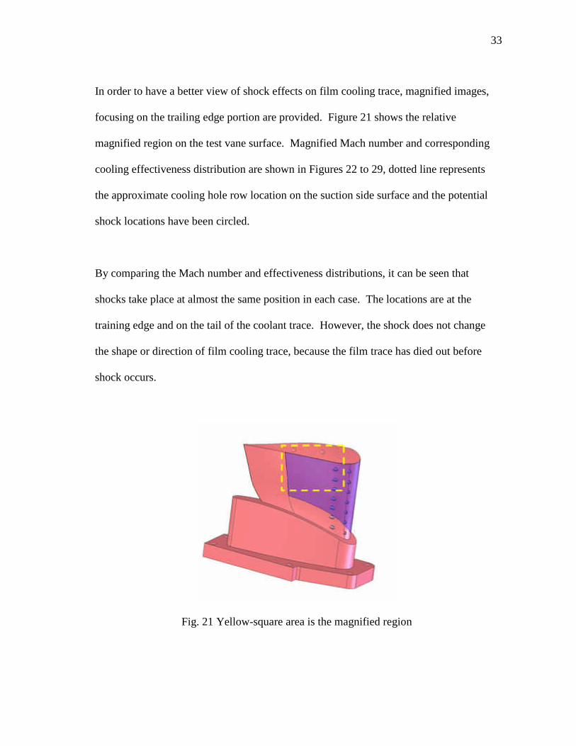
In order to have a better view of shock effects on film cooling trace, magnified images,

focusing on the trailing edge portion are provided. Figure 21 shows the relative

magnified region on the test vane surface. Magnified Mach number and corresponding

cooling effectiveness distribution are shown in Figures 22 to 29, dotted line represents

the approximate cooling hole row location on the suction side surface and the potential

shock locations have been circled.

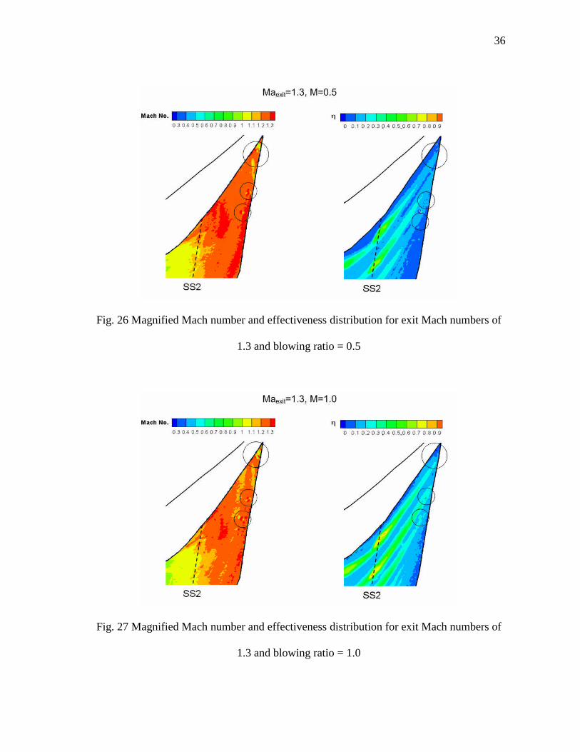
By comparing the Mach number and effectiveness distributions, it can be seen that

shocks take place at almost the same position in each case. The locations are at the

training edge and on the tail of the coolant trace. However, the shock does not change

the shape or direction of film cooling trace, because the film trace has died out before

shock occurs.

Fig. 21 Yellow-square area is the magnified region

34

Fig. 22 Magnified Mach number and effectiveness distribution for exit Mach numbers of

1.1 and blowing ratio = 0.5



35





36





37





38

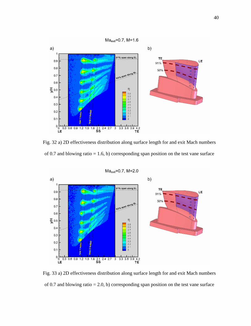
Figures 30 to 41 show the 2D contour plots of film cooling effectiveness, this provides

more clear and better pictures for the coolant trace and the effectiveness level. For

subsonic condition, M = 1.0 has the optimum effectiveness. For supersonic condition, M

= 1.6 provides the optimum cooling effectiveness. Further increase of blowing ratio

causes the narrower traced and resulting in less coverage and lower effectiveness. This

is due to the increase of momentum as the blowing ratio increases, and causes the

coolant jet liftoff. The inclined hub portion of test vane performs as a nozzle and

redirects the mainstream flow; due to horseshoes vortices and secondary flow effects, the

film cooling trace near the hub has been bended upward.

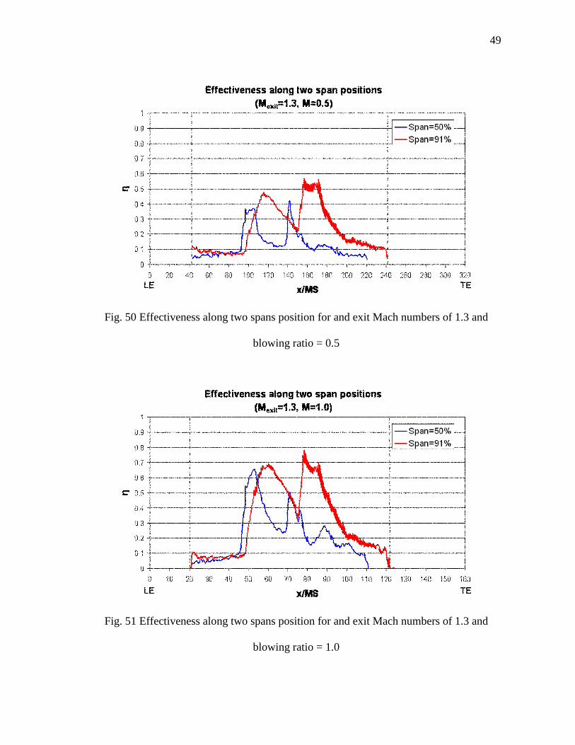
Figures 42 to 53 show the averaged effectiveness for the four blowing ratios and three

mainstream velocities. The effectiveness data is plotted for non-dimensional distance of

x/MS – the downstream distance (x) divided by the blowing ratio (M) and equivalent

slot width (S). This parameter is used to try to correlate the data for all blowing ratios

onto one curve. The plots are given for 50% and 91% of span surface length. The 50%

span pass through the middle film cooling hole from row 1 and row 2; the 91% span pass

through the first film cooling hole from the top of row 1 and row 2. Two major peaks on

91% span indicate two film cooling holes from row 1 and row 2; 50% span have two

major peaks and multiple small peaks, small peaks are due to the bended coolant trace

near the hub portion.

39

Fig. 30 a) 2D effectiveness distribution along surface length for and exit Mach numbers

of 0.7 and blowing ratio = 0.5, b) corresponding span position on the test vane surface



40





41





42





43





44





45

Fig. 42 Effectiveness along two spans position for and exit Mach numbers of 0.7 and

blowing ratio = 0.5


blowing ratio = 1.0

46


blowing ratio = 1.6


blowing ratio = 2.0

47


blowing ratio = 0.5


blowing ratio = 1.0

48


blowing ratio = 1.6


blowing ratio = 2.0

49


blowing ratio = 0.5


blowing ratio = 1.0

50


blowing ratio = 1.6


blowing ratio = 2.0

51

Overall Comparison

Figure 54 and Figure 55 show the comparison of the film cooling effectiveness of three

different mainstream velocities and four different blowing ratios. At low blowing ratio

(M=0.5), exit Mach number = 0.7 has greatest effectiveness follow by the order of exit

Mach number = 1.1 and 1.3; as blowing ratio increases, the effectiveness looks similar

for supersonic exit conditions.

The spanwise averaged film cooling effectiveness for different exit Mach number and

blowing ratios are plotted in Figures 56 to 59. There are two major peaks , which

indicates two film cooling holes from row 1 and row 2; at low blowing ratio (before

reaching the optimum value), the second peak is higher than the first peak duo to the

coolant accumulation downstream. At high blowing ratio (after reaching the optimum

value), the second peak becomes lower because the coolant shoot into the mainstream.

The optimum blowing ratio for supersonic exit condition is 1.6; however, the optimum

blowing ratio for subsonic condition is 1.0. This is due to the interaction between shock

and free stream turbulence. The interaction causes the increasing pressure and assists

the coolant to attach on the blade surface at higher blowing ratio; besides, the secondary

flow effect decreases as mainstream velocity increases. Thus, the supersonic cases

perform better than the subsonic case.

52

Fig. 54 Effectiveness comparison of exit Mach number = 0.7 to 1.3 and blowing ratio =

0.5 and 1.0

53

Fig. 55 Effectiveness comparison of exit Mach number = 0.7 to 1.3 and blowing ratio =

1.6 and 2.0

54

Fig. 56 Spanwise averaged effectiveness comparison of blowing ratio = 0.5


SS1 SS2

SS1 SS2

55



SS1 SS2

SS1 SS2

56

CONCLUSIONS

As exit Mach number becomes 1.1 and 1.3, shockwaves occur at the near-to-trailing

edge region and the tail of the coolant trace on the test vane surface. Results show that

shocks do not change the trace shape and direction because the coolant dies out before

the shocks take place.

On the suction side surface, based on two rows of compound angle shaped holes, the

cooling effectiveness increases as blowing ratio increases, till it reaches the critical

blowing ratio = 1.0 (for subsonic) and 1.6 (for supersonic). Further increase of blowing

ratio causes the coolant liftoff and detach from the vane surface, thus the effectiveness

drops. Effects of blowing ratio can also be seen from the 2D line plots by comparing the

first and second peak.

As a result of: (1) High pressure caused by shock, not only assists the coolant jet to

against the blade surface at higher blowing ratio but also damp the mainstream

turbulence . (2) Secondary flow effects decrease as mainstream velocity increases. The

optimum film cooling effectiveness happens at M=1.6 (with shock) and at M=1.0

(without shock).

57

REFERENCES

[1] Han, J.C., Dutta, S., and Ekkad, S., 2000, Gas Turbine Heat Transfer and Cooling

Technology, Taylor and Francis, New York.

[2] Goldstein, R.J., Eckert, E.G., and Burggraf, R., 1974, “Effects of Hole Geometry and

Density on Three Dimensional Film Cooling,” Int. J. of Heat and Mass Transfer,

17, pp. 595–606.

[3] Sen, B., Schmidt, D.L., and Bogard, D.G., 1996, “Film Cooling with Compound

Angle Holes: Heat Transfer,” ASME J. Turbomachinery, 118, pp. 800–806.

[4] Schmidt, D.L., Sen, B., and Bogard, D.G., 1996, “Film Cooling with Compound

Angle Holes: Adiabatic Effectiveness,” ASME J. Turbomachinery, 118, pp. 807–

813.

[5] Thole, K., Gritsch, M., Schulz, A., and Wittig, S., 1998, “Flowfield Measurements

for Film Cooling Holes with Expanded Exits,” ASME J. Turbomachinery, 120, pp.

327–336.

[6] Gritsch, M., Schulz, A., and Wittig, S., 1997, “Adiabatic Wall Effectiveness

Measurements of Film-Cooling Holes With Expanded Exits,” IGTI Conference,

Orlando, pp. 97-GT-164.

[7] Yu, Y., Yen, C., Shih, T., Chyu, M., and Gogineni, S., 1999, “Film Cooling

Effectiveness and Heat Transfer Coefficients Distributions around Diffusion

Shaped Holes,” IGTI Turbo Expo, The Hahue, The Netherlands, pp. 97-GT-312.

58

[8] Gao, Z., Narzary, D., and Han, J., 2007, “Film-Cooling on a Gas Turbine Blade

Pressure Side or Suction Side With Compound Angle Shaped Holes,” ASME pp.

HT-2007-32098.

[9] Goldstein, R.J., Eckert, E.G., Eriksen, V.L., and Ramsey, J.W., 1970, “Film Cooling

Following Injection Through Inclined Circular Tubes,” Israel Journal of

Technology, 8, pp. 145-154.

[10] Cho, H.H., Rhee, D.H., and Kim, B.G., 2001, “Enhancement of Film Cooling

Performance Using a Shaped Film Cooling Hole with Compound Angle Injection,”

JSME International Journal, Series B, 44, No. 1, pp. 99-110

[11] Saumweber, C., Schulz, A., and Wittig, S., 2003, “Free-Stream Turbulence Effects

on Film Cooling With Shaped Holes,” ASME J. Turbomachinery, 125, pp. 65-73.

[12] Kadotani, K., and Goldstein, R. J., 1979, ‘‘On the Nature of Jets Entering a

Turbulent Flow Part A: Jet-Mainstream Interaction,’’ASME J. Eng. Power, 101,

pp. 459–465.

[13] Kadotani, K., and Goldstein, R. J., 1979, “On the Nature of Jets Entering a

Turbulent Flow Part B: Film Cooling Performance,” ASME J. Eng. Power, 101, pp.

466–470.

[14] Mehendale, A.B., and Han, J.C., 1992, “Influence of High Mainstream Turbulence

of Leading Edge Film Cooling Heat Transfer,” ASME Journal of Turbomachinery,

114, pp. 707-715.

59

[15] Burd, S. W., Kaszeta, R. W., and Simon, T. W., 1998, “Measurements in Film

Cooling Flows: Hole L/D and Turbulence Intensity Effects,’’ASME J.

Turbomachinery, 120, pp. 791–797.

[16] Gau, Z.Nazary, D., Mhetras, S., and Han, J., 2007, “Full Coverage Film Cooling for

a Turbine Blade with Axial Shaped Holes,” AIAA Paper No. AIAA-2007-3402.

[17] Pedersen, D.R, Eckert, E.R.G., and Goldstein, R.J., 1997, “Film Cooling with Large

Density Differences Between the Mainstream ans Secondary Fluid Measured by

the Heat-Mas Transfer Analogy,” ASME Journal of Heat Tranfer, 99, pp. 620-627.

[18] Sinha, A.K., Bogard, D.G., and Crawford, M.E., 1991, “Film Cooling Effectiveness

Downstream of a Single Row of Holes with Variable Density Ratio,” ASME

Journal of Turbomachinery, 113, pp 442-449.

[19] Mhetras, S., and Han, J., “Effect of Unsteady Wake on Full Coverage Film-Cooling

Effectiveness for a Gas Turbine Blade,” ASME/AIAA Joint Heat Transfer

Conference, San Francisco, May 2006.

[20] Mhetras, S., and Han, J., “Effect of Superposition on Spanwise Film-Cooling

Effectiveness Distribution on a Gas Turbine Blade,” ASME IMECE 2006-18084.

60

VITA

Kuo-Chun Liu is from Taipei, Taiwan, and received his Bachelor of Science degree in

mechanical engineering from Kansas State University in May, 2007. In September 2007,

he began his graduate study in Texas A&M University. While in graduate study at

Texas A&M University, he worked in the turbine heat transfer laboratory as a research

assistant with Dr. J.C. Han. Liu graduated with his Master of Science degree in

mechanical engineering (August, 2009) and is continuing on to pursue his Ph.D. in the

same field of study.

Mailing Address:

Kuo-Chun Liu

Department of Mechanical Engineering

c/o Dr. J.C. Han

Texas A&M University

College Station, TX, 77843-3132

BLOWING RATIO EFFECTS ON FILM COOLING...

Documents

Transcript of BLOWING RATIO EFFECTS ON FILM COOLING...