A Framework to Identify Greater Sage-grouse Preliminary Priority Habitat and Preliminary General

Habitat for Idaho

Paul Makela-Wildlife Biologist and Don Major-Landscape and Fire Ecologist U.S. Bureau of Land Management

Idaho State Office Resources and Science Branch

Boise, Idaho

April 2012

2

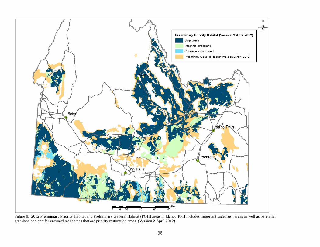
Executive Summary In September 2011, Idaho BLM completed initial efforts to model greater sage-grouse (sage-grouse) priority areas and general areas (PAs and GAs) for Idaho, using Western Association of Fish and Wildlife Agencies’ Sage-grouse Management Zone IV for the analysis boundary, to provide regional context. This initial effort mapping effort is referred to hereinafter after as Version 1, and is described in detail in Chapter 1. The delineation of PAs in Version 1 was based solely on sage-grouse breeding bird (lek) density and lek connectivity models described in the literature. Sage-grouse GAs were modeled using BLM’s Currently Occupied Habitat map and a sage-grouse population persistence model, which is essentially an index of sagebrush cover on the landscape. Version 1 was used during winter 2012 for public scoping for BLM and U.S. Forest Service (FS) sage-grouse planning strategy effort. While the Version 1 map provided a repeatable means for displaying sage-grouse preliminary priority areas based on lek information, additional internal discussions and input from local and regional sage-grouse experts and others identified a need for refinements. This led to an update, referred to hereinafter as Version 2, described in detail in Chapter 2. In Version 2, the terms Preliminary Priority Habitat and Preliminary General Habitat (PPH/ PGH) were formally adopted, to provide consistency with terminology in BLM national policy. New information incorporated into Version 2, includes 1) additional lek data, 2) seasonal habitat information, 3)identified movement and migration corridors, 4) addition of local sage-grouse priority areas of the Challis Local Working Group, 5) areas of habitat connectivity, 6), incorporation of refinements suggested by the U.S. Forest Service, and 7) exclusion of modeled agricultural and timber lands. In addition to refining the sagebrush components of PPH and PGH in greater detail in Version 2, we also incorporated certain potential restoration habitats as a subset of PPH. Many of these areas, currently characterized as perennial grasslands or conifer encroachment areas, have recently undergone (or may, in the foreseeable future) various efforts to enhance or restore habitat extent or improve connectivity. The final, overall map for PPH/PGH Version 2 is shown in Chapter 2, Figure 8. Figure 9 provides additional detail regarding the various vegetation categories of PPH including sagebrush, perennial grassland and conifer encroachment. To facilitate future discussions of possible conservation actions or activities within PPH and PGH, Chapter 3 provides general suggestions for consideration. Depending on the nature and extent of sage-grouse habitat conditions locally and on the broader landscape, conservation efforts in some PPH or PGH areas may require more of a focus on habitat maintenance, to retain current habitat values. Conversely, other areas may require more of a focus on habitat improvement or restoration. Alternative approaches or strategies for management of PPH/PGH may also be identified as BLM and conservation partners move forward with sage-grouse conservation efforts.

3

Introduction In March 2010, U.S. Bureau of Land Management (BLM) Washington Office Instruction Memorandum (IM) 2010-071 (Bureau of Land Management 2010) directed field office managers to implement appropriate conservation actions in priority sage-grouse habitat. Subsequent guidance (Washington Office IM 2012-043) provided interim conservation measures for use within preliminary priority habitat (PPH) and preliminary general habitat (PGH) areas, while BLM is amending land use plans. PPH is defined as areas that have been identified as having the highest conservation value to maintaining greater sage-grouse populations; PGH is defined as areas of occupied seasonal or year-round habitat outside of priority habitat. The purpose of this paper is 1) to document the background, rationale and processes used in identifying greater sage-grouse (sage-grouse) PPH and PGH for Idaho; and, 2) to describe preliminary considerations for use of this information in conservation planning. Many areas of sage-grouse habitat in Idaho are contiguous with habitats in the neighboring states of Utah, Nevada, Oregon, and Montana. Therefore we chose to use the Western Association of Fish and Wildlife Agencies (WAFWA) Sage-grouse Management Zone IV (MZ IV; Figure 1) as the primary analysis boundary, to provide a regional context for Idaho’s PPH and PGH. While MZ IV encompasses the vast majority of the sage-grouse habitat in Idaho, it excludes habitat in the Bear Lake Plateau area located in the extreme southeastern portion of the state. This area is associated with WAFWA MZ II (Wyoming Basin) so PPH/PGH in that part of Idaho was identified separately. It should be noted that due to the regional scale of the analysis and nature of the modeling techniques used, PPH and PGH may encompass inclusions of non-habitat especially at finer, more local scales. Consequently, additional information including local knowledge will be necessary when planning more site specific conservation efforts and in interpreting PPH/PGH. The process leading to the most current (April 2012) PPH/PGH map involved two versions. Version 1 was completed in September 2011, and relied solely on sage-grouse breeding bird density and lek connectivity information for delineating priority areas. Early in the process we assigned the terms “Priority Area” (PA) and “General Area” (GA) for simplicity. These labels are retained in the forthcoming discussion and associated map figures for Version 1 to maintain the integrity of the original documentation, metadata and map labels. Version 1 also was used as the basis for Idaho’s PPH/PGH map shown during public scoping for BLM’s sage-grouse planning strategy in winter 2012. Version 2 was completed in April 2012, following scoping, and incorporated additional important information provided by Idaho Department of Fish and Game, BLM, US Forest Service and others, including sage-grouse seasonal habitats, movement corridors, habitat connectivity, locally important leks and telemetry data. Version 2 also incorporates filters for agriculture and timber lands, excluding those areas from PPH/PGH, and more closely aligns with Idaho’s “Sage-grouse Habitat Planning Map” which has been in use since 2000, for general conservation planning purposes. Overall, Version 2 provides a more detailed and comprehensive

4

portrayal of preliminary PPH/PGH in the state, and is intended to replace Version 1 in its entirety. Background-Related Mapping Efforts Other sage-grouse habitat mapping efforts over the past decade have guided sage-grouse conservation planning in Idaho, and provide important context for the sage-grouse habitat mapping/modeling efforts described in this document. Idaho Sage-grouse Habitat Planning Map: In 2000, Idaho BLM drafted “A Framework to Assist in Making Sensitive Species Habitat Assessments for BLM-Administered Public Lands in Idaho- Sage-grouse” (Sather-Blair et al. 2000). This document, released to Idaho BLM field offices via Idaho BLM IM 2000-059 (Bureau of Land Management, 2000) outlined recommended field protocols for assessing sage-grouse habitats and also described a process for mapping sage-grouse habitat and potential restoration areas at the broad scale, to aid in conservation planning in the state. The resulting Idaho Sage-grouse Habitat Planning Map (sometimes referred to informally as the “Key habitat map”) has been updated annually since that time, based primarily on wildfire polygons, expert opinion and/or other new information. However, this map displays only general habitats (i.e., key habitat, defined as areas of generally in-tact sagebrush that provide sage-grouse habitat during some portion of the year, and potential restoration areas comprised of perennial grasslands, annual grasslands and conifer encroachment areas.). It does not reflect the relative importance or priority of those habitat areas with respect to sage-grouse population characteristics. Sage-grouse Strongholds and Isolated Populations: Additional state and federal agency collaborative mapping efforts in Idaho during the past decade identified sage-grouse population areas assumed to be “strongholds” or “isolated populations”, based on local biological expertise and lek information. This map was briefly utilized by Idaho BLM and conservation partners as a means to identify potentially important population areas as well as several presumed isolated populations. However, this map was never updated from the original version (c.a. 2002) due to a lack of adequate sage-grouse population-level information, and has since been abandoned pending the availability of more suitable and defensible population data and analytical techniques.

Seasonal Habitat Models: In 2006, the Idaho Sage-grouse Advisory Committee (SAC) completed the “Conservation Plan for the Greater Sage-grouse in Idaho” (State Plan; Idaho Sage-grouse Advisory Committee 2006), which incorporated recent science and conservation measures into a more comprehensive state-level sage-grouse conservation plan. Recognizing the limitations of the Idaho Sage-grouse Habitat Planning Map, the SAC recommended in a 2009 update to Chapter 6 of the State Plan, that Idaho “continue to explore and review emerging remote-sensing tools and products that would have the capability and accuracy to refine or replace the Sage-grouse Habitat Planning Map.” As a follow-up to that recommendation, Idaho BLM and Idaho Department of Fish and Game (IDFG) embarked on a Challenge Cost Share project in 2010 to model sage-grouse general habitat and seasonal habitats using telemetry, observational, land cover and climatic data. These spatial models (Knetter et al., in progress) may be useful in future refinements to sage-grouse habitat maps and models.

5

Breeding Bird Density: To provide a more consistent analytical foundation and to further promote the mapping of sage-grouse priority habitats at the state level, the BLM Washington Office in 2010 entered into an Assistance Agreement with the U.S. Fish and Wildlife Service (FWS) to model sage-grouse “breeding bird density”, or “BBD” at three scales: 1) across the range of the species; 2) by WAFWA sage-grouse management zone; and 3) by individual state, following Doherty et al. (2011).

6

Chapter 1: Version 1- September 2011- Modeling Sage-grouse Priority and General Areas (PAs and GAs) Study Area: Stiver et al. (2006) identified seven “sage-grouse management zones” (Figure 1) within the geographic distribution of the greater sage-grouse, based on sage-grouse populations and subpopulations occurring within seven floristic provinces (Connelly et al. 2004). These zones reflect ecological issues and similarities conducive to more effective and efficient conservation planning. Idaho is almost entirely within MZ IV with the exception of a small corner of southeastern Idaho. Zone IV also includes portions of southwestern Montana, northwestern Utah, northern Nevada and southeastern Oregon. While Idaho comprises the majority of MZ IV, numerous sage-grouse leks and potentially important habitats and populations/subpopulations occur in proximity to Idaho’s border in the adjoining MZ IV states. Therefore, Idaho BLM chose to expand its priority area analysis to incorporate available sage-grouse and habitat information for those adjoining states. This approach has important conservation implications in that it incorporates aspects of interstate population and habitat connectivity that would be overlooked if we limited the scale of analysis to Idaho. A regional approach to sage-grouse conservation planning such as this warrants consideration by other states that are a part of multi-state WAFWA management. Methods and Results: A primary goal in modeling draft PAs and GAs was to integrate currently available population and habitat data and current modeling techniques into a transparent and repeatable framework. A second goal was to ensure that the draft PAs and GAs were driven by the biology and ecology of sage-grouse. Lek data were acquired, with permission, from state wildlife agencies within MZ IV. For habitat data, BLM Idaho used the BLM currently occupied habitat (COH) model (Durtsche et al. 2009) and assumed for purposes of this analysis that the COH product provides a reasonable portrayal of occupied sage-grouse habitat across the range of the species. Other seamless sage-grouse habitat models were not available however new habitat models can be considered and incorporated into the PA analysis as they become available. In modeling sage-grouse PAs, BLM Idaho used 1) a Breeding Bird Density (BBD) index of sage-grouse abundance based on male attendance at leks, and 2) lek connectivity to inform the broader spatial distribution of leks. BLM Idaho assumed that BBD adequately informs the PA model as to the relative “importance” of areas with respect to recent breeding bird numbers. Lek connectivity informs the PA model as to the likely, longer-term connectedness between leks, assuming that leks in proximity to one another are more “connected” than those farther apart (Knick and Hanser 2011). Spatial data on sage-grouse late brood-rearing, fall or winter habitats were not readily available, and therefore not included in the model. However, given the buffers (6.4 km and 8.5 km) used in the BBD component and the 18 km window of the lek connectivity analysis, a significant portion of these non-breeding habitats are likely included. Breeding Bird Density: BBD analyses involve ranking leks by attendance (e.g. highest to lowest numbers of males) and summing the number of males until a desired percent-population threshold is met (e.g., the top 25%, 50%, 75% etc., of the population). With lek locations and

7

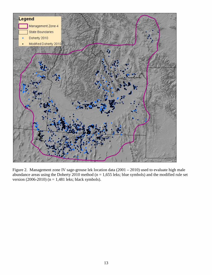
abundance being large drivers in the model, BBD results are, by definition, highly correlated with breeding habitat. We evaluated two BBD methods: 1) the original Doherty et al. (2011) model which uses a 10-year time period (2001-2010), the most recent average annual maximum lek counts, and a minimum male count =1 to identify high male abundance areas and 2) a modified Doherty version using a more restricted rule set of a 5 year time period (2006-2010), maximum lek count over the 5-yr period, and minimum male count of 2. This modified rules et incorporates the assumptions currently used to designate “occupied leks” in Idaho by IDFG. In both methods we followed the Doherty et al. (2010) lek buffering approach (add 74.6 – 76.0). Specifically, leks in the 1-75% BBD percentiles were buffered by 6.4 km (4 miles) to account for a majority of nesting areas and 76-100% BBD percentiles were buffered by 8.5 km (5.3 miles (Doherty et al. 2010 citing Holloran and Anderson 2005), since leks in those classes tend to be farther apart, in lower densities, and potentially in more fragmented habitat. We compiled 2001 – 2010 male Sage-grouse lek attendance data within MZ IV from state fish and wildlife agencies in Idaho, Nevada, Utah, Oregon, and Montana. A total of 1,655 leks were analyzed to evaluate the original Doherty et al. (2010) method and n=1,481 leks for the modified version (Figure 2). Summary statistics for both datasets were evaluated based on the average and range of male lek counts by lek and the total maximum male lek counts across all leks. While the modified Doherty method identified fewer total leks, the average male counts and total males were highest of the two datasets, better reflecting current populations. In addition, we had concerns with the longer term, ten-year dataset regarding lek location reliability, and variable survey efforts or techniques (i.e., ground vs. aerial) across MZ IV. As a result, we selected the modified Doherty method for the subsequent BBD analysis. To allow incremental examination of the entire BBD profile, we developed a Python-based model to spatially delineate BBD at 1 percent intervals. We then quantified the amount of greater sage-grouse COH using a modification of Durtsche et al. (2009) at each BBD percent to identify potential patterns or thresholds of COH and non-habitat across the entire BBD profile (Figure 3). The Durtsche et al. (2009) COH map likely underestimates habitat since COH in recent wildfires (since 2006) was omitted from this dataset. Therefore, we used burn severity data from the USGS Monitoring Trends in Burn Severity site (www.mtbs.gov) to update the COH map (Figure 4). Fire polygons (30m pixels) classified as 1=no burn, or 2=low severity were reclassified to the pre-fire land cover type and identified as either COH or not. These areas were then added to the original Durtsche et al. (2009) map. For this exercise, we assumed that areas of low burn severity retained largely the same habitat as before the burn (i.e. patchy burn with small unburned areas). Due to our limited ability to effectively characterize “burn severity” in shrub ecosystems, it is likely that COH in the low severity category is overestimated. Our results indicate no significant pattern or threshold in COH across the BBD percentage profile (Figure 3). Therefore, we examined two potential thresholds: 1) the BBD 75% value and associated proportion of COH and 2) the associated BBD percent that encompasses 80% of the COH. The 75% BBD captures approximately 60% of the available COH (~40% of available non-habitat) in MZ IV. The remaining 40% habitat (which occurs outside the 75% BBD) is likely the more fragmented habitat (Doherty et al. 2011). The 90% BBD is required to capture

8

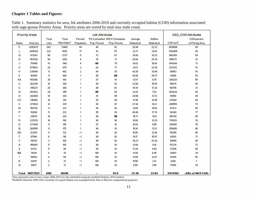
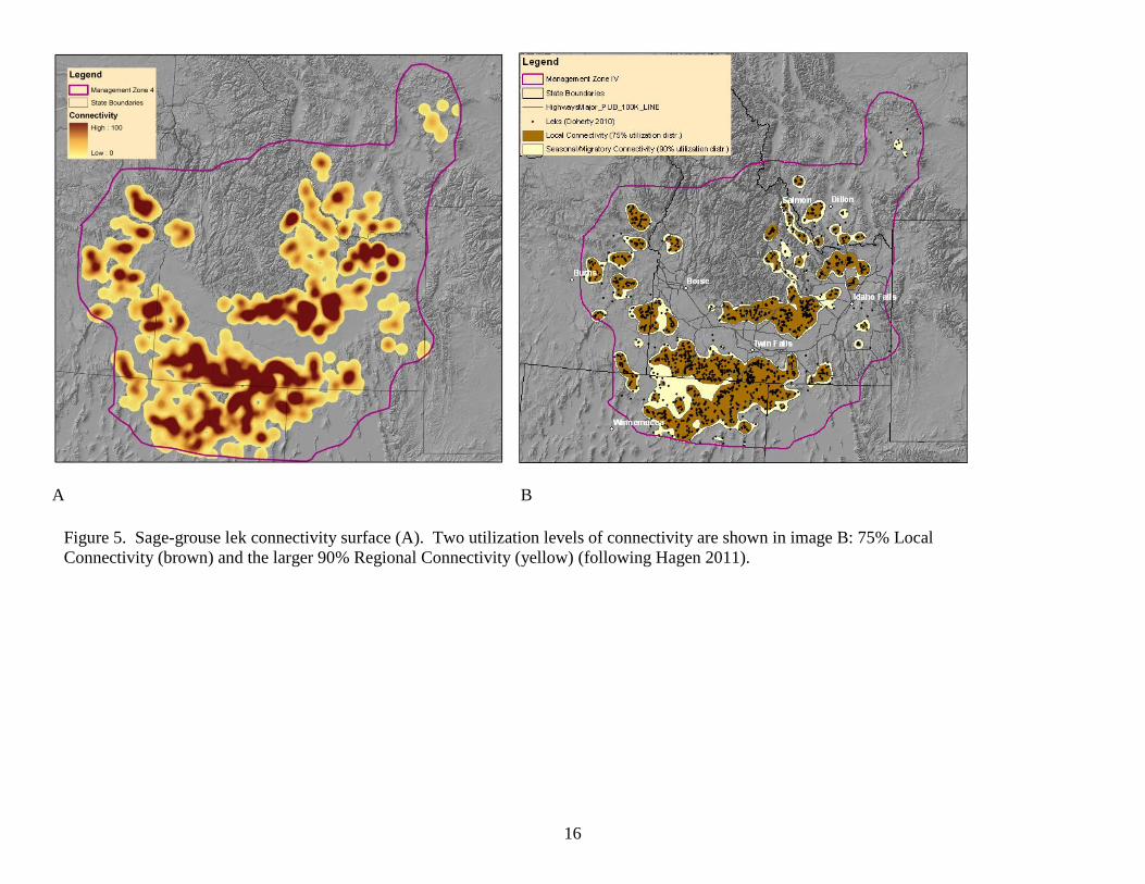
80% of available COH; however, there is a much higher proportion (70%) of non-habitat included, suggesting that the use of the 90% BBD would lead to overstating priority area boundaries. Since BBD is highly correlated with breeding habitat and the BBD 75% class captures the “top” 75% of males along with 60% of the COH, we recommend that the BBD 75% threshold be used as the “high abundance” (or “population”) component of our priority area mapping effort. This threshold provides a meaningful baseline population component for the PA analysis, by conservatively encompassing the least fragmented breeding habitats that are of greatest importance for conservation. Lek Connectivity: We used the more inclusive Doherty et al. (2010) rule set (i.e., 10 year timeframe, 1 male minimum) to identify lek points for the lek connectivity analysis. We assumed that this more comprehensive, ten-year dataset would yield a more realistic connectivity extent since the sage-grouse is a relatively long-lived bird, and the modified 5-year dataset may not be sufficient for this purpose. We used a kernel density analysis to create a utilization distribution surface. We modified Hagen (2011) and populated a 1 km grid with lek presence and analyzed kernel density using a neighborhood of 18 km. Knick and Hanser (2011) found an 18 km area to be a reliable connectivity threshold for greater sage-grouse (GSG; i.e., leks within 18 km of one another tend to be more connected than those farther out). The resulting “surface” was used to categorize 2 levels of connectivity: 75% (local connectivity) and 90% (seasonal/migratory connectivity) utilization distributions (Figure 5 A and B). Local lek connectivity (75% utilization contour) appears to encompass the “general” lek distribution patterns across MZ IV; therefore, we recommend that local connectivity be used to represent the “lek connectivity” component of our priority area mapping effort. The connectivity analysis assumed straight-line distances among lek points. Therefore, similar to the BBD analysis, some areas of non-habitat are encompassed within the resulting polygons. In addition, the connectivity analysis does not account for topography, thus overestimating connectivity results in linear basin and range systems (e.g., the Challis/Salmon area). For example, applying the 18 km connectivity neighborhood to leks occurring within narrow valley bottoms, that average only12 km in width, likely captures some adjacent areas of nonhabitat on nearby steep, timbered or rocky slopes. MZ IV Sage-grouse Priority Area Delineation: For PA delineation, we integrated aspects of “population” and “habitat”. To portray a population context, we intersected the 75% breeding density polygons with the 75% utilization local connectivity polygon (Figure 6). For context, the resulting PAs are also shown overlapping the 2010 version of the Idaho age-grouse Habitat Planning Map (Figure 7; BLM 2010b). For each PA polygon within MZ IV, we then assigned a unique alpha identification code and calculated summary statistics. Summary statistics included total polygon area, total number of leks, maximum male attendance, average maximum male attendance and standard deviation, as well as total area and percent of COH within the polygon (Table 1). We then used total maximum male attendance to rank the 30 priority area polygons. In aggregate, the PA polygons capture approximately 94% of the identified MZ IV male lek population. Additional statistics found in Table 1 are also reported to help inform future PA and GA evaluations.

9

MZ IV Sage-grouse General Area Delineation: We used sage grouse population persistence methods (modified Aldridge et al., 2008)) to inform GSG General Area delineations within MZ IV. We evaluated long-term sage-grouse population persistence as a function of sagebrush cover on the landscape. We analyzed sage-grouse population persistence based on the availability of sagebrush within a defined area, under the assumption that the modified COH model served as an adequate representation of sage-grouse habitat/sagebrush within the analysis area. Based on recent lek connectivity work (Knick and Hanser 2011), 18 km was assumed to be an effective distance for characterizing local lek connectivity over most of MZ IV. However, in the linear basin and range systems (e.g., the Challis/Salmon region in Idaho) general valley floor width was less than 18 km (range 8 – 16 km) and could potentially overestimate persistence. Therefore, we selected a smaller 12 km distance to more accurately reflect available area. We used the USGS National Hydrologic Dataset 4th order hydrologic units to identify the linear basin and range systems within MZ IV (Figure 8 A). We resampled the modified 2009 COH model (30m) to 1 km (with an inclusion threshold of 50% COH). The resulting 1 km grid cells (value 1, 0) were then analyzed using a moving window analysis and separate 12 km and 18 km neighborhoods (Figure 8 B). The resulting combined map “surface” was then used to categorize persistence probability. Areas of 25-65% probability represent Low sage-grouse population persistence over the long-term, and areas > 65% probability represent High sage-grouse population persistence (Aldridge et al. 2008) (Figure 8 B). We used a persistence threshold of ≥25% to identify the General Area polygons within MZ IV (Figure 8 C). All or portions of certain GA polygons may be important to sage-grouse in terms of connectivity between PA polygons or as refugia in the event of stochastic events in PAs. In some cases, areas are designated as GAs because lek data are lacking due to limited surveys, resulting in BBD or connectivity values that are too low to be captured by the PA model. Management Zone IV PAs and GAs shown in Figure 9 spatially depict those areas in the MZ IV landscape where sage-grouse conservation efforts might be focused to greater or lesser degrees, depending on management and policy objectives. Given limited resources, conservation efforts generally should focus first on habitats occurring within the PA areas. It must be recognized though, that given the population-centric nature of the PA model and associated analysis buffers, areas of sage-grouse habitat as well as non-habitat are included in those polygons. Consequently, finer-scale habitat information will be necessary at the local, site-specific level. It is also important to recognize that depending on the area of the map or specific PA or GA under consideration, there may be differing management opportunities, strategies, and decision-space for the conservation of sage-grouse. Portions of some PAs or GAs are likely very crucial to local or regional sage-grouse populations or for maintaining connectivity. To identify these areas, additional information is required and is discussed below, To further refine our understanding of the spatial context of PAs and GAs across MZ IV, and to facilitate discussions of potential management activities within or among these areas, we examined the contribution of a suite of variables to assist in identifying important conservation areas. We combined our continuous persistence, connectivity, and BBD model surfaces to create a single, composite view of the MZ IV landscape. We combined the full range of persistence probability (1-100%) information with lek connectivity (1-100%) and finally the BBD data (with lek counts normalized from 1-100). The resulting map (Figure 10) displays the full range of

10

surface values to help provide additional spatial context, inform conservation efforts within PA polygons, and to assist in the development of subsequent finer-scale management strategies. In Figure 10, “hotspots” of blue colors indicate those areas of greater relative “importance”, to sage-grouse in MZ IV, where the combination of lek connectivity, BBD and population persistence on the landscape appears to be comparatively high relative to other areas of the map. Priority Area and General Area Delineation for the Bear Lake Plateau (MZ II): The Bear Lake Plateau area of extreme southeastern Idaho occurs outside of the MZ IV analysis area discussed above. Due to floristic similarities and a closer association with populations and habitats in adjacent areas within Utah and Wyoming, this portion of Idaho is encompassed by the adjacent Wyoming Basin MZ II. While available sage-grouse population and habitat information for this portion of Idaho are somewhat limited, the area nonetheless contains potentially important sage-grouse habitats and populations that should be considered by conservation planners and managers in Idaho. Logistical and time limitations precluded us from developing a full MZ II analysis; therefore, we incorporated other available data to develop the PA map for this portion of southeastern Idaho. We examined BBD results (Doherty et al. 2011) for MZ II and Key Habitat data from Idaho’s 2010 Sage-grouse Habitat Planning Map. Specifically, we selected the 75% BBD polygons occurring within the Bear Lake Plateau area and merged them with the Idaho Key Habitat data. We then applied a 1 km buffer to the 75% BBD to assist in aggregating the polygons. Any Key Habitat polygons intersecting and extending beyond the 75% BBD polygon were included as part of the final Bear Lake Plateau PA (Figure 11). Remaining key habitat areas not intersected by the 75% BBD and associated 1 km buffer were designated as sage-grouse GAs. Figure 12 displays the full, composite map of MZ IV and Bear Lake Plateau PAs and GAs. Initial Delineation of Preliminary Priority and Preliminary General Habitat: On December 9, 2011, the BLM and US Forest Service published a Notice of Intent (NOI) in the Federal Register inviting the public to participate in public scoping meetings to evaluate greater sage-grouse conservation measures in land use plans throughout Idaho and Southwestern Montana, and elsewhere within the general range of the species. A sixty-day scoping period for this effort commenced on January 9, 2012. In conjunction with scoping, Idaho BLM made available to the public a map of PPH/PGH for the Idaho/SW Montana planning subregion (Figure 13). The Idaho portion of this map was derived by clipping the Idaho “PA and GA” areas of the Sage-grouse MZ IV map developed during the Version 1 mapping effort and joining them to Montana’s sage-grouse core areas. The subsequent revision of the Version 1 map is described in the Version 2 discussion later in this document.

____________________________________

11

Chapter 1 Tables and Figures: Table 1. Summary statistics for area, lek attributes 2006-2010 and currently occupied habitat (COH) information associated with sage-grouse Priority Areas. Priority areas are sorted by total max male count.

1Data represents total of max counts 2006-2010 for leks identified using the modified Doherty 2010 method. 2Modified Durtsche 2009 GSG Currently Occupied Habitat was resampled from 30m to 90m for computational purposes

12

Figure 1. Sage-grouse management zones (Stiver et al. 2006) within the geographic distribution of the greater sage-grouse, based on sage-grouse populations and subpopulations occurring within seven floristic provinces, as described in Connelly et al. (2004). The Management Zone IV analysis area includes portions of southern Idaho, southwestern Montana, northwestern Utah, northern Nevada and southeastern Oregon

13

Figure 2. Management zone IV sage-grouse lek location data (2001 – 2010) used to evaluate high male abundance areas using the Doherty 2010 method (n = 1,655 leks; blue symbols) and the modified rule set version (2006-2010) (n = 1,481 leks; black symbols).

14

Figure 3. BBD percentiles (left) ranging from dark red to light brown. The dark areas essentially show the “best of the best” areas, based on maximum count data at leks 2006-2010. The darkest areas capture the top 25% of the leks and breeding habitat; darker brown to light brown areas capture 50, 75 and 100% of the data, respectively. The graphs on the right show the relationship between Breeding Bird Density (BBD)

15

Figure 4. The Durtsche et al. (2009) Greater Sage-grouse Currently Occupied Habitat (COH) map did not include any areas of recent fire (since 2006) (red polygons). Therefore, we used Burn Severity data from USGS Monitoring Trends in Burn Severity (www.mtbs.gov) to update the map. Within fire polygons, areas (30m pixels) classified as 1=no burn, or 2-low severity were reclassified to the pre-fire land cover type and identified as either GSG COH or not. These areas were then added to the original Durtsche et al. 2009 map. Note that due to our limited ability to effectively characterize ‘burn severity” in shrub ecosystems, it is likely that we are overestimating COH in the low severity category. But for this exercise, we assumed that areas of low burn severity retained largely the same habitat as before the burn (i.e. patchy burn).

16

A B

Figure 5. Sage-grouse lek connectivity surface (A). Two utilization levels of connectivity are shown in image B: 75% Local Connectivity (brown) and the larger 90% Regional Connectivity (yellow) (following Hagen 2011).

17

Figure 6. Sage-grouse priority areas delineated in Management Zone IV. Priority areas (red) were delineated by intersecting the 75% connectivity and 75% breeding bird density (BBD) polygons. The letter in each polygon denotes the polygon “name”.

18

Figure 7. Management zone IV sage-grouse Priority Area (PA) polygons overlain on the 2010 Idaho Sage-grouse Habitat Planning Map. The red areas show key habitat (areas of generally in-tact sagebrush that provide habitat for sage-grouse at some point during the year. The green, yellow, and blue areas respectively show areas of perennial grassland, annual grassland and conifer encroachment restoration potential.

19

A B

C

Figure 8. Habitat-based sage-grouse persistence probability surface (modified Aldridge et al. 2008) for management zone IV. (A) Persistence surface represents the relative amount of GSG currently occupied habitat (COH) within an 12 km neighborhood for the identified basin and range subset (combined blue polygons) and 18 km for the remaining portion of management zone IV. (B) Combined Persistence probability categorized as Low (25-65%, light green) and high (>65%, dark green). (C) General Area designations for sage-grouse in management zone IV (data represents persistence value ≥ 25%). Priority Areas have been clipped out of the image.

20

Figure 9. Identified Greater Sage-grouse Priority Areas (PA) and General Areas (GA) in management zone IV.

21

Figure 10. Combined lek connectivity, habitat-based persistence probability, and Breeding Bird Density (BBD) data for MZ IV. Map surface colors indicate Low (light yellow) to High (dark blue) combined value rating for these three factors, overlain by sage-grouse Priority Area (PA) boundaries. Blue to dark blue areas appear to be of high relative importance for conservation and may warrant particular attention during conservation planning efforts.

22

Figure 11. Bear Lake Plateau area (MZ II). Sage-grouse Priority Area (PA) for Idaho is represented by the bright green polygon. Note the 2010 Idaho Key Habitat polygons (shaded red) that are encompassed within the green PA polygon. The colored circles represent Breeding Bird Density results (Doherty et al. 2010) for Management Zone II: 25% BBD (dark red), 50% (red), and 75% (light brown).

23

Figure 12. Draft Sage-grouse Priority Area and General Area Designations for Management Zone IV and Idaho – Bear Lake Plateau (MZ II).

24

Figure 13. Sage-grouse Preliminary Priority Habitat and Preliminary General Habitat map Provided During Scoping for the BLM Sage-grouse Planning Strategy.

25

Chapter 2: Version 2 -April 2012- Refinements to Sage-grouse Preliminary Priority Habitat (PPH) and Preliminary General Habitat ( PGH) in Idaho Introduction: In response to additional input from local and regional sage-grouse and habitat experts, new spatial data, and public comments, we initiated a refinement of the Version 1 analysis. Specifically, our refinements focused on 1) further evaluation of the population components (leks and lek counts) in the original analysis and 2) incorporation of additional data to inform the sagebrush component of PPH, including: i) seasonal habitat information (e.g., fall, winter, late brood), ii) identified movement and migration corridors, iii) addition of local sage-grouse priority areas, iv) incorporation of additional areas of habitat connectivity, v) incorporation of recommendations arising from FS review, and vi) exclusion of modeled agricultural and timber lands. In addition to revising PPH/PGH in Version 2 as described above, we also incorporated certain perennial grassland and conifer encroachment “potential restoration areas” as a subset of PPH. Many of these potential restoration habitat types have recently (or may in the foreseeable future) undergone various efforts to enhance or restore habitat extent or improve connectivity. Since these potential restoration habitats are typically intermixed with or in proximity to preliminary priority sagebrush areas, and since the potential restoration areas themselves may be used in varying degrees by grouse, managing these areas as a component of PPH may be important to the long-term sustainability of sage-grouse populations in the state. The importance of these potential restoration habitats is also underscored by the fact that Idaho appears to have lost approximately two-thirds of its sage-grouse habitat since pre-settlement times, thus emphasizing the need for ongoing restoration efforts (especially to recover sagebrush) and appropriate management of remaining habitats. Additional population information: BLM and IDFG Field staff identified a subset (n=10) of “important” high male attendance leks that were not previously captured in the Version 1 PA designations (Figure 1). All of these leks occurred within the 75% BBD coverage, however were not captured in the initial analysis because they did not intersect w/ the 75% utilization lek connectivity surface. The revised 2011PA polygons were then used to provide the foundation for the following integration of additional available sage-grouse habitat and related information, described below. Additional habitat information: A combination of Key Habitat (Sather-Blair et al., 2000; ISAC 2006; BLM 2012), recently mapped winter and/or breeding habitat (Burak and Moser 2009; NMV LWG 2011), local sage-grouse priority areas previously identified spatially by the Challis Local Working Group, known migration movement corridors, and the revised 2011PA polygons were used to further refine the Preliminary Priority Habitat (PPH) and Preliminary General Habitat (PGH) boundaries. The following criteria were used:

a. Any Key Habitat (Sather-Blair et al., 2000; ISAC 2006: BLM 2012) inclusions or portions extending

beyond the revised 2011 PA polygon boundaries were identified as PPH: 1) if the extension connected to an adjacent revised 2011 PA polygon and/or 2) extended out to the intersection of the Persistence boundary, to exclude areas of low (<25%) persistence (see Chapter 1 - MZ IV Sage-grouse General Area Delineation for Persistence discussion, and Figure 2, this chapter).

b. Any identified sage-grouse winter or breeding (Spring) habitat areas within or extending beyond the revised 2011 PA boundary were identified as PPH (Figure 3).

c. Priority Areas identified by the Challis Sage-grouse Local Working Group within or extending

beyond the revised 2011 PA boundary were identified as PPH (Figure 4).

d. Sage-grouse movement and migration areas were identified using a combination of expert opinion (primarily discussions with Dr. Jack Connelly) and telemetry location information. Telemetry data spanned a 15 - 20 year period representing targeted local sage-grouse studies and was used to

26

provide “general” support of sage-grouse movement patterns. Migration and movement areas were identified that connected revised 2011 PPH polygons as well as any identified Key habitat, crucial winter, breeding, or Local Working Group identified priority areas (Figure 5)

e. Any Key Habitat (Sather-Blair et al., 2000; ISAC 2006; BLM 2012) not connected to the revised

2011 PPH (polygons) or extending beyond the Persistence model’s 25% boundary was identified as Preliminary General Habitat (PGH).

f. Any PGH (from >25% Persistence model) occurring within the revised 2011 PA polygons was

retained as PGH. Incorporation of Potential Restoration Areas into PPH: In addition to refinement of the sagebrush component of PPH as described above, we also included certain “potential restoration” habitat types into PPH (Figure 6). These were restricted to identified perennial grasslands and areas of conifer encroachment and correspond to those areas shown in BLM 2012 (and as defined in Sather-Blair et al 2000 and ISAC 2006). The following criteria were used:

a. Any Potential Restoration area Type R1 (perennial grassland) or R3 (conifer encroachment) occurring within the revised 2011 PA polygons was identified as PPH.

b. Any R1 or R3 Habitat occurring outside the revised 2011 PA polygons was identified as Preliminary General Habitat (PGH).

Incorporation of U.S. Forest Service edits: National Forests within Idaho reviewed draft revised PPH/PGH data during April 2012. Suggested edits, based on local seasonal habitat information were provided to BLM in a geodatabase format by the FS Geospatial Technology Service Center. Polygons were attributed by the FS as either 1) breeding habitat, 2) breeding/summer/early fall habitat, 3) breeding/summer/early fall/ fall/winter habitat; 4) summer/early fall habitat or 5) summer/early fall/fall/winter habitat. We then applied the following rule set to allow for incorporation of FS edits without otherwise compromising other important components of the PPH/PGH analysis.

a. An initial assumption was made that polygons containing the terms” breeding” and/or “winter” habitat in the “season” data field, were relatively more important than other seasonal habitats, and therefore constituted PPH. Polygons with no reference to breeding or winter habitats in the “season” field and polygons where seasonal descriptors were lacking (n=3; acre total ~500) constituted PGH. Following this initial characterization, we then applied the following rule set:

i. Polygons identified as “breeding” and/or “winter” habitat were attributed as PPH. Remaining seasonal habitats were attributed as PGH.

ii. Polygons identified as PGH that intersected existing PPH were attributed as PPH.

b. If Forest Service polygons occurred within areas of migration/movement/connectivity concern, they were attributed as PPH.

Incorporation of Agriculture and Conifer Filters to Refine PPH and PGH: The final step in refining the PPH areas involved applying both an agricultural and conifer filter to exclude those areas from the final PPH product (Figure 7). Agricultural and conifer land cover types were mapped using the Landfire v1.01 land cover dataset. For computational purposes the 30m land cover data was resampled to 90m. Separate 1 km moving window analyses were used to sum agriculture and conifer occurrence, respectively across Idaho. A 25% threshold value (representing 25% occurrence in the 1 km2 window) was used as the agricultural filter. Aldridge et al. (2008) reported that sage-grouse extirpations were more likely to occur in areas where cultivated

27

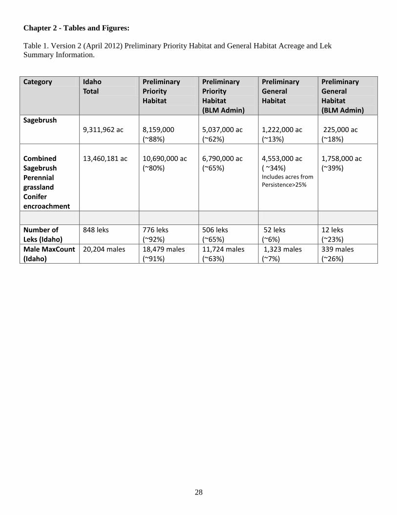
crops exceeded 25% of a 30 km landscape. A 50% threshold value (representing 50% occurrence in the 1 km2 window) was used as the conifer filter. Doherty et al. (2008) reported that sage-grouse avoided coniferous habitats at a 0.65-km2 scale. Any areas of sagebrush, perennial grass, or conifer that were contained within the above agriculture or conifer filters were incorporated into PGH to provide additional context at more local scales and to acknowledge that these edge areas or inclusions, while influenced by conifer or agriculture, may still be utilized by sage-grouse to some degree. Summary: The Version 2, April 2012 Preliminary Priority Habitat designation encompasses three subcategories of habitat including 1) sagebrush, 2) perennial grassland potential restoration areas, and 3) conifer encroachment potential restoration areas that are assumed to be relatively important for sage-grouse conservation planning efforts based on the above analysis and assumptions. Summary statistics for habitat acreages, land status, and leks are provided in Tables 1 and 2. Figure 8 displays PPH with the three subcategories merged, for simplicity, along with PGH. Figure 9 displays the three subcategories of PPH separately, in addition to PGH.

____________________________________

28

Chapter 2 - Tables and Figures: Table 1. Version 2 (April 2012) Preliminary Priority Habitat and General Habitat Acreage and Lek Summary Information. Category Idaho

Total Preliminary Priority Habitat

Preliminary Priority Habitat (BLM Admin)

Preliminary General Habitat

Preliminary General Habitat (BLM Admin)

Sagebrush

9,311,962 ac

8,159,000 (~88%)

5,037,000 ac (~62%)

1,222,000 ac (~13%)

225,000 ac (~18%)

Combined Sagebrush Perennial grassland Conifer encroachment

13,460,181 ac

10,690,000 ac (~80%)

6,790,000 ac (~65%)

4,553,000 ac ( ~34%) Includes acres from Persistence>25%

1,758,000 ac (~39%)

Number of Leks (Idaho)

848 leks 776 leks (~92%)

506 leks (~65%)

52 leks (~6%)

12 leks (~23%)

Male MaxCount (Idaho)

20,204 males 18,479 males (~91%)

11,724 males (~63%)

1,323 males (~7%)

339 males (~26%)

29

Table 2. Version 2 (April 2012) Preliminary Priority Habitat and General Habitat Land Ownership Summary. These data are for illustrative purposes only. Inclusion in PPH or PGH is partly a function of the relatively broad scale nature of the analysis, and is not intended to imply endorsement by specific land owners or agencies.

Preliminary Priority Habitat (PPH) Preliminary General Habitat (PGH) OWNERSHIP ACRES PPH % of PPH OWNERSHIP ACRES PGH % of PGH BLM 6,789,794 65 BLM 1,758,132 39 BOR 1,326 <1 BOR 21,972 <1 CORPS.

ENGINEERS 2,939 <1

DOE 377,828 4 DOE 182,455 4 HSTRCWTR 1,340 <1 HSTRCWTR 2,422 <1 INDIAN RES. 143,949 1.4 INDIAN RES. 10,672 <1 DOI Bankhead-Jones

56,507 <1 DOI Bankhead-Jones

6,916 <1

USDA Bankhead-Jones

38,025 <1 USDA Bankhead-Jones

7,862 <1

MILITARY 11,142 <1 MILITARY 37,714 <1 NPS 27,313 <1 NPS 222,669 5 NATIONAL WILDLIFE REFUGE

204 <1 NATIONAL WILDLIFE REFUGE

3,149 <1

OTHER 60,637 <1 OTHER 29,449 <1 PRIVATE 1,655,919 16 PRIVATE 1,243,058 27 STATE 616,088 6 STATE 338,264 7 STATE IDFG 23,954 <1 STATE IDFG 24,765 <1 STATE PARKS

2,178 <1 STATE PARKS 5,149 <1

USFS 715,276 7 USFS 655,635 14 MISC 168,519 1.6 GRAND TOTAL

10,690,000 100 GRAND TOTAL

4,553,224 100

30

Table 1. Version 2 (April 2012) Preliminary Priority Habitat and General Habitat Summary Information.

Figure 1. Important areas of high male lek attendance (blue circles) that were added as PPH polygons in Version 2 (April 2012). The purple/pink areas show the original (Version 1, 2011) PA/GA.

31

Figure 2. Identified Key Habitat that occurs within the revised 2011 PA polygons (red) or connects among polygons was delineated as PPH. Key habitat areas extending beyond the revised 2011 PA polygon and contained within the Persistence 25% surface (green) were also included as PPH. Other identified seasonal and/or high importance areas within or outside Key habitat were also included as PPH.

32

A-Winter

B – Breeding

Figure 3. Identified sage-grouse winter (A) and breeding (B) areas.

33

Figure 4. Identified Sage-grouse Local Working Group Priority areas.

34

A

B

Figure 5. A - Important sage-grouse movement and migration areas identified from expert opinion and telemetry location information. B – Winter (yellow) and Breeding (blue) season telemetry location used to visually examine movement and migration areas.

35

Figure 6. Perennial grasslands and conifer encroachment areas occurring within the revised 2011 PA polygons (red) were delineated as Preliminary Priority Habitat areas for the 2012 revision. Areas outside the polygons were delineated as Preliminary General Habitat. Data represents perennial grassland, conifer encroachment, and some Persistence >25%.

36

A

B

Figure 7. A – Agricultural filter: B – Conifer filter. Vegetation data was obtained from Landfire v1.01.

37

Figure 8. 2012 Sage-grouse Preliminary Priority Habitat (PPH) and Preliminary General Habitat (PGH) in Idaho. 2012 Preliminary General Habitat represents the remaining sagebrush, perennial grassland, conifer encroachment, and some Persistence >25% not accounted for in the 2012 Preliminary Priority Habitat.(Version 2 April 2012).

38

Figure 9. 2012 Preliminary Priority Habitat and Preliminary General Habitat (PGH) areas in Idaho. PPH includes important sagebrush areas as well as perennial grassland and conifer encroachment areas that are priority restoration areas. (Version 2 April 2012).

39

Chapter 3: Management Approaches for Consideration The information presented in this paper should not be construed as policy. It is primarily intended to complement and provide spatial context for interim national BLM sage-grouse policy and a framework for further conservation planning efforts. Specifically, this information can provide helpful context for analyses and decisions associated with future project-level work, authorizations, activity planning or land-use planning that may affect sage-grouse or sage-grouse habitat on BLM lands in Idaho. To inform future discussions of possible management actions for the various PPH or PGH (or portions thereof), we suggest considering two general approaches, as a starting point. Habitat Maintenance Focus: In some areas, the focus of sage-grouse habitat conservation may best be achieved by an effort to maintain or protect the current extent and health of sagebrush landscapes and sage-grouse population connectivity. These areas might include PPH or portions of PPH that currently provide relatively important, intact sage-grouse habitat and are therefore important for sustaining sage-grouse populations into the future. Examples of management actions could include: 1) the establishment of exclusion zones for certain types of actions (e.g., energy development), or sage-grouse “conservation areas”, Areas of Critical Environmental Concern, or other protective designations to minimize or reduce anthropogenic impacts; 2) application of more stringent project stipulations or protective buffers; and 3) provide aggressive and proactive approaches to wildfire suppression, establishment of strategic fuel breaks, implementation of juniper/conifer control activities, or other protective or maintenance measures appropriate for the landscape. Habitat Improvement Focus: In some areas, the focus of sage-grouse habitat conservation may best be achieved by an effort to restore the extent and ecological health of sagebrush landscapes to improve sage-grouse habitat quality, quantity and population connectivity. These would be comprised of PPH and/or PGH that currently are constrained due to concerns with habitat quality, fragmentation or other factors that could be ameliorated with restoration activities or other approaches. Management actions could focus on efforts to restore sagebrush and/or the herbaceous components of the habitat, reduce conifer expansion, and protection of restoration investments (i.e., aggressive wildfire suppression). Future Modeling Opportunities: Given the repeatable and transparent analytical framework described in earlier chapters, we can readily incorporate other geospatial landscape metrics, threat information, or other data as they become available. For example, we could incorporate information on the Human Footprint (Leu et al. 2008), or Core Patch Size Distribution using Patch Analyst for ArcGIS. Other class or landscape metrics (e.g., habitat connectivity, fragmentation or aggregation indices, edge density, etc.) could also be explored to further characterize the nature and context of our connectivity polygons. In the near future, we will have the opportunity to incorporate sage-grouse seasonal habitat models currently under development for Idaho and MZ IV by IDFG (Knetter and Svancara, in progress) using a Maximum Entropy (MAXENT) climate envelope characterization of sage-grouse habitat. We anticipate these will be helpful in further informing sage-grouse conservation at multiple scales. Acknowledgements: Many individuals provided helpful comments the various phases of this project. We would like to especially thank the following for their input: Cameron Aldridge (US Geological Survey), Jack Connelly (Idaho Dept. Fish & Game), Shawn Espinosa (Nevada Dept. Wildlife), Christian Hagen (Oregon Dept. Fish & Wildlife), Steve Hanser (US Geological Survey), Nick Hardy (US Fish & Wildlife Service), Don Kemner (Idaho Dept. Fish & Game), Sonya Knetter (Idaho Dept. Fish & Game), Steve Madsen (Utah BLM), Rick Northrup (Montana Dept. Fish, Wildlife, & Parks), Tom Rinkes (Idaho BLM), Frank Quamen (BLM National Operation Center), Robin Sell (Colorado BLM), and Kendra Womack (US Fish & Wildlife Service).

______________________

40

Literature Cited: Aldridge, C. L., S. E Nielsen, H. L. Beyer, M. S. Boyce, J. W. Connelly, S. T. Knick, and M. A. Schroeder.

2008. Range-wide patterns of greater sage-grouse persistence. Diversity and Distributions 14:983-994. Burak, G., and A. Moser. 2009. Sage-grouse Seasonal Habitat Mapping-Progress Report. Unpublished IDFG

report. Boise, ID. Bureau of Land Management. 2000. Instruction Memorandum 2000-059. Guidance implementing the draft

sage-grouse habitat assessment framework for lands administered by the Bureau of Land Management (BLM) in Idaho.

Bureau of Land Management. 2010. Instruction Memorandum 2010-071. Gunnison and greater-sage-grouse

management considerations for energy development (Supplement to National Sage-grouse Habitat Conservation Strategy).

Bureau of Land Management. 2010b. Idaho Sage-grouse Habitat Planning Map 2010 Version. Shapefile

available at http://cloud.insideidaho.org Bureau of Land Management. 2012. Idaho Sage-grouse Habitat Planning Map 2011 Version. Shapefile

available at http://cloud.insideidaho.org Connelly, J.W., S.T. Knick, M.A. Schroeder, and S.J. Stiver. 2004. Conservation assessment of greater sage-

grouse and sagebrush habitats. Western Association of Fish and Wildlife Agencies. Unpublished Report. Cheyenne, WY.

Doherty, K.E., D.E. Naugle, H. Copeland, A. Pocewicz, and J. M. Kiesecker. 2011. Energy development and

conservation tradeoffs: Systematic planning for sage-grouse in their eastern range. Pages 505-516 in S.T. Knick and J. W. Connelly, editors, Greater Sage-Grouse-Ecology and Conservation of a Landscape Species and Its Habitats. Studies in Avian Biology No. 38. Cooper Ornithological Society. University of California Press. Berkeley and Los Angeles, CA.

Doherty, K.E., J.D. Tack, J.S. Evans, and D.E. Naugle. 2010. Mapping breeding densities of greater sage-

grouse: A tool for range-wide conservation planning. BLM Completion Report. Interagency Agreement # L10PG00911.

Doherty, K.E., D.E. Naugle, B. Walker, J.M. Graham. 2008. Greater sage-grouse winter habitat selection and

energy development. J. Wildlife Manage. 72(1):187-195. Durtsche, B.M., C.J. Benson, and S.V. Stegman. 2009. A GIS-based habitat model for the greater sage-grouse

in the western United States. U.S. Bureau of Land Management Unpublished Report. National Operations Center, Denver, CO.

Hagen, C. 2011. Greater sage-grouse conservation assessment and strategy for Oregon: A plan to maintain and

enhance populations and habitat. Oregon Department of Fish and Wildlife, Bend, Oregon. Available at http://www.dfw.state.or.us/wildlife/sagegrouse/docs/20110422_GRSG_April_Final%2052511.pdf Accessed 07/05/2011.

Holloran, M.J., and S.H. Anderson. 2005. Spatial distribution of greater sage-grouse nests in relatively

contiguous habitats. Condor 107:742-752.

41

North Magic Valley Sage-grouse Local Working Group. 2011. Draft Sage-grouse Conservation Plan. Idaho Sage-grouse Advisory Committee (ISAC). 2006. Conservation Plan for the Greater Sage-grouse in

Idaho. Idaho Department of Fish and Game Unpublished Report. http://fishandgame.idaho.gov/cms/hunt/grouse/conserve_plan/

Knetter, S., L. Svancara and W. Bosworth. In Progress. Mapping seasonal sage-grouse habitats using inductive

models. Bureau of Land Management and Idaho Department of Fish and Game Challenge Cost Share project.

Knick, S.T. and S. E. Hanser. 2011. Connecting pattern and process in greater sage-grouse populations and

sagebrush landscapes. Pages 383-405 in S.T. Knick and J. W. Connelly, editors, Greater Sage-Grouse-Ecology and Conservation of a Landscape Species and Its Habitats. Studies in Avian Biology No. 38. Cooper Ornithological Society. University of California Press. Berkeley and Los Angeles, CA.

Leu, M., S. E. Hanser, and S. T. Knick. 2008. The human footprint in the West: a large-scale analysis of

anthropogenic impacts. Ecological Applications 18: 1119-1139. Sather-Blair, S., P. Makela, T. Carrigan and L. Anderson. 2000. A framework to assist in making sensitive

species habitat assessments for BLM-Administered public lands in Idaho- Sage-grouse. U.S. Bureau of Land Management unpublished report. Idaho State Office, Boise, ID.

Stiver, S. J., A.D. Apa, J.R. Bohne, S.D. Bunnell, P.A. Deibert, S.C. Gardner, M.A. Hilliard, C.W. McCarthy,

and M.A. Schroeder. 2006. Greater sage-grouse Comprehensive Conservation Strategy. Western Association of Fish and Wildlife Agencies. Unpublished Report. Cheyenne, Wyoming.