BLIND CARRIER FREQUENCY OFFSET ESTIMATION FOR MULTICARRIER SYSTEMS

A Dissertation by

Mahmoud Mohammad Qasaymeh

Master of Science in Electrical Engineering, Jordan University of Science and Technology, 2003

Bachelor of Science in Electrical Engineering, Jordan University of Science and Technology, 1997

Submitted to the Department of Electrical Engineering and Computer Science

and the faculty of the Graduate School of

Wichita State University

in partial fulfillment of

the requirements for the degree of

Doctor of Philosophy

May 2009

© Copyright 2009 by Mahmoud Qasaymeh

All rights reserved

Note that thesis and dissertation work is protected by copyright, with all rights reserved. Only the author has the legal right to publish, produce, sell, or distribute this work. Author permission is needed for others to directly quote significant amounts of information in their own work or to summarize substantial amounts of information in their own work. Limited amounts of information cited, paraphrased, or summarized from the work may be used with proper citation of where to find the original work

iii

BLIND CARRIER FREQUENCY OFFSET ESTIMATION FOR MULTICARRIER SYSTEMS

The following faculties have examined the final copy of this dissertation for form and content,

and recommend that it be accepted in partial fulfillment of the requirement for the degree of

Doctor of Philosophy with a major in Electrical Engineering.

___________________________________

Ravindra Pendse, Committee Chair

___________________________________

Edwin Sawan, Committee Member

___________________________________

Gamal Weheba, Committee Member

___________________________________

Krishna Krishnan, Committee Member

___________________________________

Rajiv Bagai, Committee Member

Accepted for the College of Engineering

________________________________

Zulma Toro-Ramos, Dean

Accepted for the Graduate School

________________________________

J. David McDonald,

Associate Provost for Research and

Dean of the Graduate School

iv

DEDICATION

To my charming wife

Heba Shatnawi

v

ACKNOWLEDGEMENT

I would like to express my appreciation to my advisors Dr. M. Sawan and Dr. R. Pendse

for their sympathetic and thoughtful support. Their insightful advice, guidance and patience were

valuable. Also I would like to thank them for their continuous support, directions and perceptive

advice. I am obliged for having huge technical direction from Dr. N. Tayem. I also wish to

extend my admiration to committee members Dr. G. Weheba, Dr. K. Krishnan, and Dr. R. Bagai

for their comments and suggestions for this research. I would like to remember my colleague Dr.

H. Gami for the hours of time we shared in the development of this work. Further, I thank all the

members in the department of EECS at Wichita State University; it was a pleasure for me to

work in this group.

I would like to express my deep appreciation for the scholarship that Tafila Technical

University/ Jordan has so generously awarded me for my doctoral studies in Electrical

Engineering here at Wichita State University. It is a great honor to be considered worthy of such

a gift. My earnest intention was to be an excellent candidate and prove your confidence in me

was warranted. Special appreciation is due to the Deans’ Council of Tafila Technical University

especially Dr. S. Al-Jufout, the Dean of Academic Research and Graduate Studies.

Special thanks are also due to my dearest Heba for her sincere patience, support, and for

accompanying with me in the long, busy days that I needed to complete this work. I like to

express my deepest gratitude to my parents, sisters, brothers, and friends for their unwavering

encouragement throughout my education.

vi

ABSTRACT

A Multicarrier Communication (MCM) system such as an Orthogonal Frequency

Division Multiplexing OFDM or Discrete Multi Tone (DMT) system has been shown to be an

effective technique to combat multipath fading in wireless communications. OFDM is a

modulation scheme that allows digital data to be efficiently and reliably transmitted over a radio

channel, even in multipath environments. OFDM transmits data by using a large number of

narrow bandwidth carriers. These carriers are regularly spaced in frequency, forming a block of

spectrum. The frequency spacing and time synchronization of the carriers is chosen in such a

way that the carriers are orthogonal, meaning that they do not cause interference to each other. In

spite of the success and effectiveness of the OFDM systems, it suffers from two well known

draw backs: large Peak to Average Power Ratio (PAPR) and high sensitivity to Carrier

Frequency Offset (CFO). The presence of the CFO in the received carrier will lose orthogonality

among the carriers and because the CFO causes a reduction of desired signal amplitude in the

output decision variable and introduces Inter Carrier Interference (ICI). It then brings up an

increase of Bit Error Rate (BER). This makes the problem of estimating the CFO an attractive

and necessary research problem. In this dissertation blind estimation techniques will be proposed

to estimate the offset parameter.

vii

TABLE OF CONTENTS

Chapter Page

1. INTRODUCTION.........................................................................................................1

1.1 Introduction......................................................................................................1

1.2 Contribution of the Dissertation.......................................................................4

1.3 Dissertation Outline………….………………………………………….........4

2. ORTHOGONAL FREQUENCY DIVISION MULTIPLEXING…………………...6

2.1 Introduction …………………………………………………………….........6

2.2 OFDM History ………………………………………………………..…......7

2.3 OFDM Advantages and Drawbacks ………………..……………..………....8

2.4 Discrete Fourier Transform ………………………………...……...……….10

2.5 Matrix Formulation of the NDFT and the NIDFT………………………….10

2.6 Orthogonality Principle …………………………………………………….11

2.7 OFDM Transmitter …………………………………………………………13

2.8 Cyclic Prefix ………………………………………………………………..15

2.9 Multipath and Fading Channel ………………………………………….….17

2.9.1 Mathematical Modeling ……………….………………………...18

2.9.2 Power Delay Profiles …………………..………………............. 18

2.9.3 Frequency Selective and Flat Fading ……………………………21

2.9.4 Fast and Slow Fading.....................................................................21

2.9.5 OFDM Channel Model ………………………………………….22

2.10 OFDM Receiver.............................................................................................23

3. CARRIER FREQUENCY OFFSET ESTIMATION ………….……..……………..27

3.1 Introduction ……………………………………………………………........27

3.2 Blind CFO Estimators Based on the Used Carriers………………...……….29

3.3 Blind CFO Estimation using ESPRIT Algorithm………………….....……. 31

3.4 Blind CFO Estimation using MUSIC…………………………………….....33

3.5 Blind CFO Estimation Using Propagator Method…………………………..34

3.6 Blind CFO Estimation Using Rank Revealing QR Factorization…………...34

4. The PROPAGATOR METHOD…………………………………..……………...…35

4.1 Introduction…………………………………………………………….……35

4.2 Propagator Formulation …………………….………………………………37

4.3 CFO Problem Formulation………………………………………………….38

4.4 CFO Simulations Results………………….……………………………..….41

4.5 Conclusions …………………………………..…………………………….46

viii

TABLE OF CONTENTS (continued)

Chapter Page

5. RANK REVEALING QR METHOD………………..…………………………...…48

5.1 Introduction…………………………...…….………………………….……48

5.2 RRQR Method………... …………………….………………………………48

5.3 CFO Simulations Results …………………………………………………....50

5.4 Conclusion ………………….……………………………..……………..….53

6. CONCLUSION…..………………………………………….…….........................…54

REFERENCES………………………..…………………………..........................…56

ix

LIST OF FIGURES

Figure Page

2.1 Schematic picture of the orthogonal subcarriers ……………………………...…12

2.2 Simple OFDM Transmitter ………………………………...……………………13

2.3 Multipath environment……………………………………...……………………17

2.4 Simple OFDM receiver…………………………………………………..………23

2.5 Parallel channels via OFDM …………………………………………………….26

3.1 Schematic picture of the orthogonal subcarriers in the existence of the CFO …..28

4.1 Normalized MSE for propagator method versus structure parameter M

using K=2, 4, 6, 8, 10, 20, 30, 40, MC=200 and fixed 10 dB SNR……...………42

4.2 Normalized MSE for ESPRT method versus structure parameter

M using K=8, 10, 20, 30, 40, MC=200 and fixed 10 dB SNR………….……….43

4.3 Normalized MSE for ESPRT method versus structure parameter

M using K=2, 4, 6 MC=200 and fixed 10 dB SNR ………………………..……44

4.4 PM and ESPRIT Estimators performance versus SNR using

K=2, 4, 6, 8, 10, 20, 30 with optimal structure parameter……………………….45

4.5 PM and ESPRIT estimators performance versus the number of blocks ………...45

4.6 PM and ESPRIT estimators performance versus different………………………46

5.1 Normalized MSE versus SNR at � � 0.1�……………………………………..51

5.2 Normalized MSE versus block acquisition…………………………………...….52

5.3 Normalized Processing time versus block acquisition…………………………...52

x

LIST OF ABBREVIATIONS

4G Fourth-Generation

A/D Analog-to-Digital

ADSL Asymmetric DSL

AWGN Additive White Gaussian Noise

BER Bit Error Rate

BEWE Bearing Estimation Without Eigen decomposition

BICM Bit Interleaved Coded Modulation

CDMA Code Division Multiple Access

CFO Carrier Frequency Offset

CIR Channel Impulse Response

CM Constant Modulus

CP Cyclic Prefix

D/A Digital-to-Analog

DAB Digital Audio Broadcasting

DFT Discrete Fourier Transform

DMB-T/H Digital Multimedia Broadcast-Terrestrial/Handheld

DMT Discrete Multi Tone

DOA Direction of Arrival

DS Doppler spread

DSL Digital Subscriber Line

DTMB Digital Terrestrial Multimedia Broadcast

DVB Digital Video Broadcasting

xi

LIST OF ABBREVIATIONS (continued)

ESPRIT Rotational Invariance Technique

EVD Eigen Value Decomposition

FDM Frequency Division Multiplexing

FFT Fast Fourier Transform

FIR Finite Impulse Response

FM Frequency Modulation

GSM Global System for Mobile communications

HDTV High-Definition Television

IBI Inter Block Interference

ICI Inter Carrier Interference

IFI Inter Frame Interference

ISI Inter Symbol Interference

LANs Local Area Networks

LOS Line Of Sight

LTE Long Term Evolution

MCM Multi Carrier Modulation

MIMO Multiple-Input Multiple-Output

ML Maximum Likelihood

MSE Mean Square Error

MUSIC MUltiple SIgnal Classification

NDFT Normalized Discrete Fourier Transform

NIDFT Normalized Inverse Discrete Fourier Transform

xii

LIST OF ABBREVIATIONS (continued)

NLOS Non Line Of Sight

OFDM Orthogonal Frequency Division Multiplexing

OFDMA Orthogonal Frequency Division Multiple Access

OPM Orthonormal PM

OQAM Orthogonal Quadrature Amplitude Modulation

P/S Parallel /Serial

PAPR Peak to Average Power Ratio

PDP Power Delay Profiles

PM Propagator Method

PSK Phase Shift Keying

QAM Quadrature Amplitude Modulation

RRQR Rank Revealing QR

SC-FDMA Single Carrier Frequency-Division Multiple Access

SDARS Satellite Digital Audio Radio Services

SNR Signal-to-noise ratio

STBC Space Time Block Coding

SVD Singular Value Decomposition

SWEDE Subspace Methods Without Eigen Decomposition

TDMA Time Division Multiple Access

VC Virtual Carrier

VDSL Very high data rate DSL

VLSI Very Large Scale Integration

1

CHAPTER 1

Overview

1.1 Introduction

Technology and system requirements in the telecommunications field are changing very

fast. Over the previous years, since the transition from analog to digital communications, and

from wired to wireless, different standards and solutions have been adopted, developed,

implemented and modified, often to deal with new and different business requirements. Today,

more and more, telecommunication network operators struggle to provide new advanced services

in an attractive and functional way.

Wireless communications [1]-[4] is a rapidly growing piece of the communications

manufacturing, with the potential to provide high-speed high-quality information exchange

between the portable devices located anywhere in the world. Potential applications enabled by

this technology include multimedia Internet-enabled, Global System for Mobile (GSM), smart

homes, automated highway systems, video teleconferencing and distance learning, and

autonomous sensor networks, just to name a few. However, supporting these applications using

wireless techniques creates a significant technical challenge.

The motion in space of a wireless receiver operating in a multipath channel results in a

communications link that experiences small-scale fading. The rapid fluctuations of the received

power level due to small sub-wavelength changes in receiver position are described as small-

scale fading [4]. Basically, mobile radio communication channels are time varying, multipath

fading channels [3], [4]. In a radio communication system, there are many paths for a signal to

pass through from a transmitter to a receiver. Sometimes there is a direct path where the signal

travels without being obstructed, which is known as a Line Of Sight (LOS) path. In most cases,

2

components of the signal are refracted by different atmospheric layers or reflected by the ground

and objects between the transmitter and the receiver such as vehicles, buildings, and hills, which

is known as Non Line Of Sight (NLOS) paths. These components travel in different paths of

different length and combine at the receiver. Thus, signals on each path suffer different

transmission delays and attenuation due to the finite propagation velocity. The combination of

these signals at the receiver results in a destructive of constructive interference, depending on the

relative delays involved. In fact, the environment changes with time which leads to signal

variation. This is called time variant environment. Also, the motion of the object influences

signals. A short distance movement can cause an obvious change in the propagation paths and

vary the strength of the received signals.

Orthogonal Frequency Division Multiplexing (OFDM) [5]-[10] has been shown to be an

effective technique to combat multipath fading in wireless communications. OFDM is a

modulation scheme that allows digital data to be efficiently and reliably transmitted over a radio

channel, even in multipath environments. OFDM transmits data by using a large number of

narrow bandwidth carriers. These carriers are regularly spaced in frequency, forming a block of

spectrum. The frequency spacing and time synchronization of the carriers is chosen in such a

way that the carriers are orthogonal, meaning that they do not cause interference to each other.

OFDM has been adopted by standardization bodies and major manufacturers for a wide

range of applications. In Europe, OFDM was first standardized for Digital Audio Broadcasting

(DAB) in 1995 [11], [21] and terrestrial Digital Video Broadcasting (DVB) in 1997 [22]. OFDM

has already been used in a variety of applications, High-Definition Television (HDTV)

broadcasting [12], [13], high bit rate Digital Subscriber Line (DSL), Asymmetric DSL (ADSL)

[14], Very high data rate DSL (VDSL) [15], IEEE 802.11, multimedia mobile access

3

communications wireless Local Area Networks (LANs) [19], [20], Fourth-Generation (4G)

wireless mobile communications and Satellite Digital Audio Radio Services (SDARS). It has

recently been proposed for use in radio-over fiber based links [16] and in free-space optical

communications [17], [18]. In 2007, the first complete Long Term Evolution (LTE) air interface

implementation was demonstrated, including Multiple-Input Multiple-Output OFDM (OFDM-

MIMO), Single Carrier Frequency-Division Multiple Access (SC-FDMA) and multi-user MIMO

uplink.

OFDM can be combined with many protocols and algorithms. For example, OFDM can

be combined with multiple access schemes, such as Time Division Multiple Access (TDMA), to

achieve efficient bandwidth utilization in presence of multiple users. According to the standard

IEEE 802.16, for example, both OFDM-TDMA and Orthogonal Frequency Division Multiple

Access (OFDMA) have been adopted at 2–11 GHz band [23]. OFDM can be combined with

Space Time Block Coding (STBC) and Bit Interleaved Coded Modulation (BICM) to form

BICM-STBC-OFDM that achieves the maximum diversity [24].

In spite of the success and effectiveness of the OFDM systems, it suffers from two well

known draw backs: large Peak to Average Power Ratio (PAPR) and high sensitivity to Carrier

Frequency Offset (CFO). The presence of the CFO in the received carrier will lose orthogonality

among the carriers and because the CFO causes a reduction of desired signal amplitude in the

output decision variable and introduces Inter Carrier Interference (ICI). It then brings up an

increase of Bit Error Rate (BER) [30]- [35]. The effect caused by CFO for an OFDM/QAM

system was analyzed in [32], and it was indicated that CFO should be less than 2% of the band

width of subchannel to guarantee the signal to interference ratio be higher than 30 dB.

4

1.2 Dissertation Contributions

The estimation of the CFO is a classical problem, and it can be estimated via data added

or non-blind algorithms [36]-[44], semi blind algorithms [45], and non data added or blind [46]-

[65] algorithms. In this dissertation, the CFO blind estimation algorithms for OFDM systems

have been studied. This dissertation focuses on the blind subspace CFO estimator performance.

Two novel blind subspace CFO estimators [64], [65] have been proposed. The proposed

algorithms were tested with different applications like joint time delay and frequency estimation

problem [26], [27], and in channel estimation for the frequency hopping systems [28], [29].

1.3 Dissertation Outline

Chapter One introduces the dissertation and the contributions of the dissertation. Chapter

Two provides the concept of OFDM, history of OFDM, mathematical system model, OFDM

signal generation, multipath model, and channel classification. Chapter Three introduces one of

the major drawbacks of the OFDM system which is the carrier synchronization or what known as

carrier frequency offset. A brief summary of the different synchronization algorithms are also

presented. Chapter Four proposes a blind CFO estimator where no training pilots or reference

symbols are used. The development is proposed through the propagator method, where the

classical matrix decomposition is avoided. It is well known that subspace estimation techniques

are relying on the eigenvalue decomposition of the covariance matrix to extract the noise and/or

the signal subspace. As a result, a significant reduction in the calculation is achieved by applying

the propagator method. Chapter Five presents another blind CFO estimator based on the rank

revealing QR factorization. The RRQR is a special QR factorization that is guaranteed to reveal

the numerical rank of the matrix under consideration. This makes the RRQR factorization a

5

useful tool in the numerical treatment of many rank-deficient problems in numerical linear

algebra. It is well known that the computational load of the RRQR method is insignificant

compared with Eigen Value Decomposition (EVD) or Singular Value Decomposition (SVD) of

the cross-spectral matrix of received signals. Finally, conclusions and future work are presented

in Chapter Six.

6

CHAPTER 2

Orthogonal Frequency Division Multiplexing (OFDM)

2.1 Introduction

Frequency Division Multiplexing (FDM) is a scheme in which several signals are

combined for transmission on a single communications line or channel. Each signal travels

within its own unique carrier frequency range, which is modulated by the data [8] - [10]. In this

case, the carrier signals are referred to as subcarriers, for example, a television channel is divided

into subcarrier frequencies for video, color, and audio on the same conductors. Another example,

DSL use different frequencies for voice and for upstream and downstream data transmission

[14]. There are always some idle frequency spaces between channels, known as guardband. FDM

is famously known as Multi Carrier Modulation (MCM). FDM was the first multiplexing system

to enjoy wide scale network deployment, and such systems are still in use today [9].

OFDM spread spectrum technique distributes the data over a large number of carriers that

are spaced apart at particular frequencies. This spacing offers the orthogonality in this technique

which avoids the demodulators from seeing frequencies other than their own [10]. The OFDM

transmission scheme is the optimum version of the multicarrier transmission scheme. The

benefits of OFDM are high spectral efficiency, resistance to RF interference, and lower multi-

path distortion [6]. This is helpful because in a classic terrestrial broadcasting scenario there are

multipath-channels. Since multiple versions of the signal interfere with each other, Inter Symbol

Interference (ISI) appears. In order to afford robustness to multipath fading, OFDM is

compatible with utilizing frequency diversity. OFDM split the wideband signal into several

narrowband signals, each of which is practiced to flat fading channel instead of frequency

selective fading channel.

7

2.2 OFDM History

Researchers first published the concept of using parallel data transmission using FDM in

1966. Early in 1970 a United States patent was issued. The idea of the patent was to employ

parallel data streams and frequency division multiplexing with overlapping subchannels to avoid

the use of high speed equalization and to handle the impulsive noise, and to prevent the

multipath distortion as well as to fully use the existing bandwidth. The early applications were in

military communications. In the telecommunications area, the terminologies of Discrete Multi

Tone (DMT) and Multi Channel Modulation (MCM) are broadly used, and frequently they are

exchangeable with OFDM [5], [10].

For a large number of subchannels, the arrays of sinusoidal generators and coherent

demodulators requested in a parallel system became unreasonably expensive and complicated.

The receiver needs an accurate phasing of the demodulating carriers and sampling times in order

to keep crosstalk between subchannels at an acceptable level. The modulation and demodulation

process were implemented by applying the Discrete Fourier Transform (DFT) to parallel data. In

addition to eliminating the banks of subcarrier oscillators and coherent demodulators required by

FDM, a complete digital implementation could be built around special purpose hardware

performing the Fast Fourier Transform (FFT). Recent development in Very Large Scale

Integration (VLSI) technology allows making high speed chips that can achieve large size FFT at

affordable prices.

In the 1980s, OFDM was considered for digital mobile communications, high density

recording, and high speed modems. In the 1990s, OFDM was exploited for wideband data

communications over mobile radio Frequency Modulation (FM) channels, Asymmetric Digital

Subscriber Lines (ADSL, 1.5 Mb/s) [14], High bit rate Digital Subscriber Lines (HDSL, 1.6

8

Mb/s), Very High-Speed Digital Subscriber Lines (VHDSL, 100 Mb/s) [15]. OFDM has been

successfully used in the European DAB [11], DVB systems, HDTV terrestrial broadcasting [12],

and IEEE 802.11a-1999 or 802.11a [25].

In the 2000s, OFDM was implemented in the Digital Terrestrial Multimedia Broadcast

(DTMB) [13]. The standard was formerly named as Digital Multimedia Broadcast-

Terrestrial/Handheld (DMB-T/H). This standard was applied in China, and covers both fixed and

mobile terminals. It will eventually serve more than half of the television viewers there,

especially those in suburban and rural areas. OFDM was implemented in the DVB - Handheld

(DVB-H). In addition, the first complete Long Term Evolution (LTE) air interface

implementation was demonstrated, including OFDM-MIMO, Single Carrier FDMA (SC-

FDMA), and multi user MIMO uplink.

2.3 OFDM Advantages and Drawbacks

The OFDM is a promising transmission scheme, which has been considered extensively, as it

has the following key advantages [5]-[10]:

• OFDM makes efficient use of the spectrum.

• OFDM becomes more resistant to frequency selective fading than single carrier systems

by converting the frequency selective fading channel into narrowband flat fading

subchannels.

• OFDM eliminates Inter Symbol Interference (ISI) and Inter Frame Interference (IFI)

through use of a Cyclic Prefix (CP).

• OFDM recovers the symbols lost due to the frequency selectivity of the channel by using

adequate channel coding and interleaving.

9

• OFDM makes channel equalization simpler than single carrier systems by using adaptive

equalization techniques.

• OFDM seems to be less sensitive to sample timing offsets in comparison with single

carrier systems.

• OFDM provides good protection against co channel interference and impulsive parasitic

noise.

• OFDM makes it possible to use Maximum Likelihood (ML) decoding with reasonable

complexity. OFDM is computationally efficient with FFT techniques.

The several advantages of the OFDM systems could only appear if the main three drawbacks

were treated carefully. OFDM has the following negative aspect:

• OFDM signal has a noise like amplitude with a very large dynamic range; therefore, it

requires RF power amplifiers with a high peak to average power ratio, which may require

a large amplifier power back off and a large number of bits in the Analog to Digital

(A/D) and Digital to Analog (D/A) designs.

• OFDM is very sensitive to Carrier Frequency Offset (CFO) caused by Doppler effect.

Hence, CFO should be estimated and cancelled completely.

• OFDM receiver suffers from the difficulty to make a decision about the starting time of

the FFT symbol.

10

2.4 Discrete Fourier Transform

The Normalized Discrete Fourier Transform (NDFT) sinusoids are given by:

����� � �√ . �� ���/ (2.1)

The NDFT sinusoids are forming an orthonormal sinusoidal basis signals satisfy:

� �����, ������ � � �����. �������� ���

� �����, ������ � �1, � � �0, � �! The NDFT of a time domain signal "#�$ is given by:

%#�$ & '()*+"#�$, & �√ ∑ "#�$����� ��./0123 , � � 0,1,2, … , ' 6 1 (2.2)

The operation of the NDFT can be inverted to recover a time-domain signal from its

frequency representation. This is done with the Normalized Inverse Discrete Fourier Transform

(NIDFT). The NIDFT is given by:

"#�$ & '7()*+%#�$, & 1√' � %#�$����� �� ���

� � 0,1,2, … , ' 6 1 (2.3)

2.5 Matrix Formulation of the NDFT and the NIDFT

The NDFT and the NIDFT can be formulated as a complex matrix multiply. Based on

(2.2) and (2.3) we may write the following:

8999: %�0� %�1� %�2� ; %�' 6 1�<==

=> � 1√' .8999:?��.� ?��.� ?��. ; ?��.����

?��.� ?��.� ?��. ; ?��.����

?� .� ?� .� ?� . ; ?� .����

………@…?�����.� ?�����.� ?�����. ; ?�����.���� <==

=> .8999: "�0� "�1�"�2�; "�' 6 1�<==

=>

11

8999: "�0� "�1�"�2�; "�' 6 1�<==

=> � 1√' .8999:?�.� ?�.� ?�. ; ?�.����

?�.� ?�.� ?�. ; ?�.����

? .� ? .� ? . ; ? .����

………@…?����.� ?����.� ?����. ; ?����.���� <==

=> .8999:%�0� %�1� %�2� ; %�' 6 1�<==

=>

Define the NIDFT matrix A as:

A � �√ .8999:?�.� ?�.� ?�. ; ?�.����

?�.� ?�.� ?�. ; ?�.����

? .� ? .� ? . ; ? .����

………@…?����.� ?����.� ?����. ; ?����.���� <==

=> (2.4)

where ? � �� �/, the matrix A is a unitary matrix of size L×L, and AB. A � C. We may

write the NDFT and the NIDFT as:

X� AB. D (2.5)

x� A. E (2.6)

where the time domain data vector is D and the frequency domain data vector is E. Equations

(2.5) and (2.6) represent the matrix version of the equations given by (2.2) and (2.3).

2.6 Orthogonality Principle

OFDM is considered as a block transmission technique. In the baseband, complex-valued

data symbols modulate a large number of closely collected carrier waveforms. The transmitted

OFDM signal multiplexes a number of low rate data streams, and each data stream is associated

with a given subcarrier. The main benefit of this concept in a radio environment is that each of

the data streams deals with an almost flat fading channel. In slowly fading channels, the ISI and

Inter Carrier Interference (ICI) within an OFDM symbol can be avoided with a small loss of

12

Figure 2.1 Schematic picture of the orthogonal subcarriers.

transmission energy using the concept of the CP. An OFDM signal consists of N orthogonal

subcarriers modulated by N parallel data streams. Each baseband subcarrier ���F� is of the form

���F� � �� �G1H, � � 1,2,3, … , '

where J� is the frequency of the �HK subcarrier. The subcarrier frequencies J� are equally spaced

as:

J� � �'* which makes the subcarriers ���F� on 0 L F L '* orthogonal on each other

� ���F�, ���F�� � �'*, � � �0, � �! Figure 2.1 also shows the orthogonality among five subcarriers.

13

2.7 OFDM Transmitter

Figure 2.2 shows the block diagram of a simple OFDM transmitter. The OFDM signal is

obtained by using the orthogonal filters

M��F� � N�F�. ��� ��H/OP, � � 0,1,2, … , Q 6 1

where N�F� is a rectangular time window, Q is the number of the input symbols, and * is the

symbol transmission time. The time window is given by:

N�F� � R 1√Q* 0 L F L Q*0 �ST� U The �HK transmitted signal (corresponding to the �HK frame) can be formulated as:

"��F� � � T��. M��F 6 �Q*� O�����

where T�� is the �HK symbol to be transmitted in the �HK frame. The stream of data belonging to a

Phase Shift Keying (PSK) or QAM is Serial to Parallel (S/P) converted. Let VW��� is the

�HKblock of size P to be transmitted.

VW��� � #T���� T���� … … TO�����$P

Figure 2.2 Simple OFDM Transmitter.

Input

Symbols

S/P IDFT

VC

P/S

CP/ZP

14

To avoid aliasing problems at the receiver, N-P subcarriers at the edge of the spectrum

are not used. Thus, the vector VW of size P will be extended to the vector V of size N, by padding

N-P zeros, which is known as Virtual Carrier (VC) or unused carriers.

V��� � 899:T���� T���� … … TO�����XYYYYYYYZYYYYYYY[O , 0,0, … ,0XYZY[�OXYYYYYYYYYYZYYYYYYYYYY[ <=

=>P (2.7)

The vector V��� is fed to the N-point IDFT unit. The output vector (of size N) of the

IDFT unit for each block, which is called “time domain” block vector, is given by:

x(k)=ABV��� (2.8)

D��� � #"���� "���� … … "�����$P

We may write (2.8) as:

x(k)=AOVO��� (2.9)

Where AO is the first P column of the matrix A and given by:

AO � 1√' .8999:?�.� ?�.� ?�. ; ?�.����

?�.� ?�.� ?�. ; ?�.����

? .� ? .� ? . ; ? .����

………@…?�O���.� ?�O���.� ?�O���. ; ?�O���.���� <==

=>

AO � #\O� \O� \O … \OO��$ (2.10)

where \O� is the �HK column of AO .

15

2.8 Cyclic Prefix

Two difficulties take place when the OFDM signal is transmitted over a dispersive

channel. One difficulty is that channel dispersion destroys the orthogonality between subcarriers

and causes ICI. In addition, a system may transmit multiple OFDM symbols in a series so that a

dispersive channel causes ISI between successive OFDM symbols. The insertion of a guard

period between successive OFDM symbols would avoid ISI in a dispersive environment, but it

does not avoid the loss of the subcarrier orthogonality. The cyclic prefix (CP) both preserves the

orthogonality of the subcarriers and prevents ISI between successive OFDM symbols.

Consequently, equalization at the receiver is very simple. This frequently encourages the use of

OFDM in wireless systems. To eliminate ISI almost totally, a guard time is established for each

OFDM symbol. To avoid multipath components from one symbol to interfere with the next

symbol (ISI), the guard time that is selected should be larger than the expected delay spread.

The CP is a copy of the last samples from the IFFT, which are placed at the beginning of the

OFDM frame. More precisely, there are two reasons to insert a CP:

1. The convolution between the channel impulse response and the data will operate like a

circular convolution instead of a linear one. Circular convolution makes equalization

easier.

2. Interference from the previous symbol will only have an effect on the CP, which is not

needed in the receiver.

Both reasons assume that the CP is longer than the channels impulse response. If the CP is

shorter than the impulse response, the convolution will not be circular and ISI will arise.

However, if the number of samples in the CP is large, the data transmission rate will decrease

significantly since the CP does not carry any useful data.

16

At the output of the IFFT, a guard symbols of length '] is inserted at the beginning of

each block. In other words, the vector in (2.6) is extended by '] symbols to form either Cyclic

Prefix Orthogonal Frequency-Division Multiplexing (CP-OFDM) or Zero Padding Orthogonal

Frequency Division Multiplexing (ZP-OFDM).

D^_ � `"�a , … … "��XYYYYZYYYY[a, "�, "� … , "�a , … "��XYYYYYYZYYYYYY[ b (2.11.a)

Dc_ � R"�, " … … "��XYYYZYYY[ , 0,0, … … 0XYYZYY[aU (2.11.b)

Due to the cyclic extension or zero padding, the efficiency of OFDM transmissions

reduces by a factor of da after a redundant '] symbols are inserted between each D���. The

resulting blocks D^_ or Dc_ are finally sent sequentially through the channel. The total number of

time-domain samples per transmitted block is ' e '] . Thus, it is important to choose the

minimum possible CP to maximize the system efficiency. The guard symbols also eliminate the

need for a pulse-shaping filter, and it reduces the sensitivity to time synchronization problems.

The CP/ZP can be added by extending the NIDFT matrix to AOfO / AOgOof size (' e ']� h Q

AOfO � 1√' .8999999:?�.� ?�.��a� ?�.��a� … ?�O���.��a� ?�.� ; ?�.� ?�.� ?�. ;

?�.��ad�� ?�.��ad�� …; ; …?�.� ?�.� …?�.� ?�.� …?�. ?�. …; ; …

?�O���.��ad�� ; ?�O���.� ?�O���.� ?�O���. ; ?�.���� ?�.���� ?�.���� … ?�O���.���� <======>

AOfO � i\OfO� \OfO� \OfO … \OfOO��j (2.12.a)

AOgO � �√ . kl�mnT�'] h Q�AO o (2.12.b)

17

where \OfO� is the �HK column of AOfO . In this thesis the CP-OFDM is considered. We may write

(2.8) as:

Dpq��� � AOfO . VO��� (2.13)

2.9 Multipath and Fading Channel

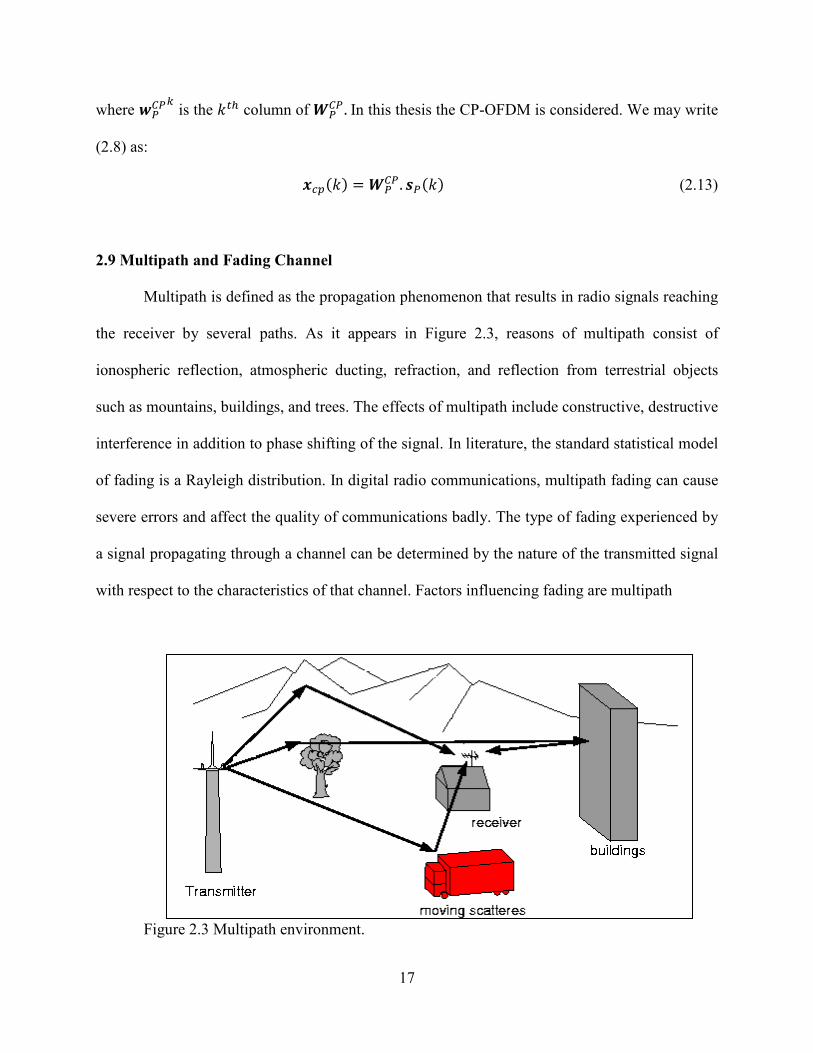
Multipath is defined as the propagation phenomenon that results in radio signals reaching

the receiver by several paths. As it appears in Figure 2.3, reasons of multipath consist of

ionospheric reflection, atmospheric ducting, refraction, and reflection from terrestrial objects

such as mountains, buildings, and trees. The effects of multipath include constructive, destructive

interference in addition to phase shifting of the signal. In literature, the standard statistical model

of fading is a Rayleigh distribution. In digital radio communications, multipath fading can cause

severe errors and affect the quality of communications badly. The type of fading experienced by

a signal propagating through a channel can be determined by the nature of the transmitted signal

with respect to the characteristics of that channel. Factors influencing fading are multipath

Figure 2.3 Multipath environment.

18

propagation environment, the speed of the mobile, the speed of the surrounding objects, and the

bandwidth of the transmitted signal.

2.9.1 Mathematical Modeling

A simple mathematical model can be presented by assuming that the transmitted signal is

an ideal pulse at time zero. At the receiver, due to the presence of the multiple electromagnetic

paths, several pulses will be received; thus, each one of them will arrive at different times. In

fact, since the electromagnetic signals travel at the speed of light, and since every path has a

length probably different from that of the others, there are different traveling times. Thus, the

received signal will be expressed by:

r�F� � "�F� � s�F� � � t�

����� . ��u2 . v�F 6 w��

where N is the number of received pulses which is exactly the number of possible paths, and may

be very large number, τn is the time delay of the �HK pulse, and t���u2 represents the complex

amplitude (magnitude and phase) of the received pulse. By definition, y(t) represents the impulse

response function h(t) of the equivalent multipath model. In general, the consideration of time

variation of the geometrical reflection conditions yields an impulse response that varies with

time.

2.9.2 Power Delay Profiles

Power Delay Profiles (PDP) are generally modeled as plots of relative received power as

a function of excess delay with respect to a fixed time delay reference. The maximum delay time

spread parameter is used to denote the severity of multipath surroundings. It is also called the

19

multipath time *x, and it is defined as the time delay existing between the first and the last

received impulses. The delay spread is the square root of the second central moment of the

power delay profile and given by:

y � zw {{{ 6 �w|� where

}~{{{ � ∑ W�}��. }�~ �∑ W�}�� �

w| � ∑ Q�w��. w� �∑ Q�w�� � }{ is the first moment of the PDP known as the mean excess delay. Typical values of delay spread

are on the order of microseconds in outdoor mobile radio channels and on the order of

nanoseconds in indoor radio channels. The multipath can be characterized by either the channel

transfer function H(f), or the impulse response h(t), where they are related to each other by the

continuous time Fourier transform

��J� � � s�F���� �GH�F���

� � t���u2����� ��� �G�2

The obtained multipath channel transfer function characteristic has a typical appearance of a

sequence of peaks (maxima) and notches (minima); it can be shown that, on average, the

distance in Hertz between two consecutive peaks is roughly inversely proportional to the

multipath time. The coherence bandwidth is defined as:

�p � �*x

20

The coherence bandwidth is defined to be the range of frequencies over which two frequencies

have possiblety for amplitude correlation [2]. If two sinusoids with a frequency separation of

greater than Bc are propagating in the same channel, they are affected quite differently by the

channel. Delay spread and Coherence bandwidth describe perfectly the time dispersive nature of

the channel. They do not offer any information about the time varying nature of the channel

caused by the relative motion of the transmitter and/or the receiver.

Doppler spread (DS) is a measure of spectral expansion caused by motion, the time rate of

change of the mobile radio channel, and is defined as the range of frequencies over which the

received DS is essentially non-zero. It offers information about the fading rate of the channel.

Knowing DS in mobile communication systems can improve detection and help to optimize

transmission at the physical layer, as well as higher levels of the protocol stack. If the baseband

signal bandwidth is much less than the DS, then effect of the DS is negligible at the receiver.

Doppler spread (�, is defined as the maximum Doppler shift and given by:

(� � J� � ��

Coherence time is inversely related to DS. Coherence time is defined to be the time

duration over which the channel impulse response is mainly invariant with time [1]. If the

symbol time of the baseband signal is larger than the coherence time, then the signal will distort,

since the channel will change during the transmission of the single symbol time. Doppler Spread

and coherence time are parameters which express the time varying nature of the channel in a

small-scale region. By definition, Coherence time implies that two signals arriving with a time

separation greater than *p are affected differently by the channel.

21

2.9.3 Frequency Selective and Flat Fading

By comparing the channel coherence bandwidth and the signal bandwidth, the channel

can be classified into frequency selective fading or flat fading. In frequency selective fading, the

coherence bandwidth of the channel is smaller than the bandwidth of the signal [3]. Different

frequency components of the signal therefore experience uncorrelated fading. In a frequency-

selective fading channel, because different frequency components of the signal are affected

separately, it is highly doubtful that all parts of the signal will be simultaneously affected by a

deep fade. Some modulation techniques such as OFDM and Code Division Multiple Access

(CDMA) are compatible with employing frequency diversity to offer robustness to selective

fading. OFDM divides the wideband signal into several narrowband subcarriers, each of which

are practiced to flat fading instead of frequency selective fading. The length of the CP is chosen

for the maximum anticipated multipath spread; for the IEEE 802.11a standard, this is 25% of

OFDM symbol duration, indicating a significant loss in utilization. In flat fading, the coherence

bandwidth of the channel is larger than the bandwidth of the signal, and the symbol period of the

transmitted signal is much larger than the Delay Spread of the channel. Therefore, all frequency

components of the signal will be subjected to the same magnitude of fading.

2.9.4 Fast and Slow Fading

Slow fading scenario arises when the channel coherence time is larger than the channel

delay constraint. In this scenario, the channel can be considered roughly constant over the period

of use, the amplitude and phase change are small enough to be neglected. Slow fading can be

founded by events such as shadowing, where a large obstruction such as a hill or large building

obscures the main signal path between the transmitter and the receiver [4]. Fast fading occurs

when the coherence time of the channel is small relative to the delay constraint of the channel

22

[2]. In this system, the amplitude and phase change imposed by the channel varies considerably

over the period of use. In a fast fading channel, the transmitter may take advantage of the

variations in the channel conditions by using time diversity to help increase the robustness of the

communication system.

2.9.5 OFDM Channel Model

In OFDM systems, the CP length needs to be larger than the maximum excess delay of

the channel. If this information is not available, the worst case channel condition is used for

system design, which makes CP a significant portion of the transmitted data, thus reducing

spectral efficiency. One way to increase spectral efficiency is to adapt the length of the cyclic

prefix depending on the radio environment. This adaptation requires an estimation of the

maximum excess delay of the radio channel, which is also related to the frequency selectivity of

the channel. Other OFDM parameters that could be changed adaptively using the knowledge of

the dispersion are OFDM symbol duration and OFDM subcarrier bandwidth. The CP length is

assumed to be known or pre-estimated. The channel can be represented by an equivalent discrete

time model and its effects can be represented by a linear Finite Impulse Response (FIR) filter

with the Channel Impulse Response (CIR):

^ � #��, ��, � , … , ����, 0,0,0, … ,0$ The channel transfer function H(z) is given by:

���� � ∑ ��. �./023������ , � � 0,1,2, … , ' 6 1

� �� e ��. �� �/ e � . ����/ … e ����. �� ������/ (2.14)

Using the matrix notation, let

B � AB. ^

23

� #��0�, ��1�, ��2�, … , ��'�$P

� #s�, s , s�, … , s$P (2.15)

2.10 OFDM Receiver

The CP is added between each OFDM block in order to transform the linear convolution into a

circular convolution. After Parallel to Serial (P/S) and Analog to Digital (A/D), the signal is sent

through a frequency selective channel. The block diagram of the OFDM receiver is shown in

Figure 2.4. For noiseless received signals and given channel state information, reversed steps to

the transmitter operation are applied. The discrete time received signal with CP guard interval,

denoted as �fO, is given by the following expression:

�fO �89999: m�fO���m fO���;;;mdafO ���<=

===>

� ����.89999:"�a���;"�����"����;"����� <==

==> e ����.89999:"�a�� 6 1�;"���� 6 1�"��� 6 1�;"���� 6 1� <==

==>

� ����. Dpq��� e ����. Dpq�� 6 1� (2.16)

where ���� represents inter-symbol interference generated by the frequency selective behavior of

Figure 2.4 Simple OFDM receiver

OFDM

block

S/P DFT

VC

P/S

CP/ZP

24

the channel inside an OFDM block at time k. ���� is a square matrix of size �' e ']� h �' e']� and is given by:

���� corresponds to Inter Block Interference (IBI) between two consecutive block transmissions

at k and k + 1 and given by:

At the receiver end, in order to cancel the IBI, the first '] samples of the frame are discarded.

899999:m�dafO ���m dafO ���;;;mdafO ���<==

===>

�89999:m����m ���;;;m���<==

==> � ����� … �� 0 @ @0 @ @���� … ��

� . D��� (2.18)

This can be rewritten as:

25

89999:

�� 0 …; @ @���� @���� … �� @ ;@ ����0 @ ; @ @0 … 0

@ @ ; @ 0���� … �� <====> . A�.

89999:

T����;TO�����00 <==

==> (2.19)

The use of cyclic redundancy has enabled us to convert the linear convolution to a circular

convolution. Since any circulant matrix is diagonal in the Fourier basis [16], it is very easy to

diagonalize the channel effect by FFT processing at the receiver as shown below:

8999: r����r����;r�����r��� <=

==> � A.

89999:m����m ���;;;m���<==

==> � A.89999:

�� 0 …; @ @���� @���� … ��@ ;@ ����0 @; @ @0 … 0

@ @ ;@ 0���� … �� <====> . A�

XYYYYYYYYYYYYZYYYYYYYYYYYY[B

.89999:

T����;TO�����00 <==

==>

� ����#s�, s , s�, … , s$. V

� ����#s�, s , s�, … , sO$. VW (2.20)

r���� � s�T���� From the simple properties, convolution in one domain is equivalent to multiplication in the

other domain. Convolution here yields a multiplication in the frequency domain. The signal s is

transmitted over N parallel flat fading channels. Each channel is subjected to complex frequency

attenuation. As shown in Figure 2.5. In the case of noisy transmission, the time Gaussian added

noise vector is multiplied at the receiver by the FFT demodulator, the statistics of a Gaussian

vector does not change by orthogonal transformation.

26

.

Figure 2.5 Parallel channels via OFDM.

T� r� s�

e

�� h

T r s

e

�

h

T r

s

e

�

h

27

CHAPTER 3

Carrier Frequency Offset Estimation

3.1 Introduction

OFDM is a great technique to handle impairments of wireless communication channels

such as multipath propagation. Hence, OFDM is a practical candidate for future 4G wireless

communications techniques [1] - [4]. On the other hand, one of the major drawbacks of the

OFDM communication system is the drift in reference carrier. The offset present in received

carrier will lose orthogonality among the carriers as shown in Figure 3.1. Hence, the CFO causes

a reduction of desired signal amplitude in the output decision variable and introduces ICI. Then it

brings up an increase of BER. The effect caused by CFO for OFDM system was analyzed in

[30]-[35]. In [30] BER upper bound of OFDM system is analyzed without ICI self cancellation

[31] and BER of OFDM system is analyzed using self cancellation, but this method is less

accurate. In [33], it is indicated that CFO should be less than 2% of the bandwidth of the

subchannel to guarantee the signal to interference ratio to be higher than 30 dB. A critically

sampled OFDM/OQAM system is also not robust to CFO [33], even when optimal pulses are

used as shaping filters [34]. Thus, carrier frequency offset greatly degrades system performance.

Therefore, practical OFDM systems need the CFO to be compensated with sufficient accuracy,

and this has led to a whole lot of literature on CFO estimation algorithms. In [35], a formula for

the BER analysis of OFDM system with the conjugate cancellation scheme has been derived.

Most of the existing CFO estimators for OFDM are based on periodically transmitted

pilot symbols [36] - [41]. Yet, the pilot symbols transmission loses a significant bandwidth,

especially in the case of continuous transmissions. Therefore, pilot-based schemes are mainly

suited for packet oriented applications.

28

Figure 3.1 Schematic picture of the orthogonal subcarriers in the existence of the

CFO.

Semi blind approaches proposed in the literature are the first step to improve the

bandwidth efficiency [45]. Those usually depend on various assumptions such as the usage of a

single pilot symbol, two identical consecutive OFDM data blocks, or some specific structure

within the OFDM symbol.

Recently, blind, or non data aided methods have received extensive attention, as the

bandwidth will be totally kept for real data. Among different classes of blind methods, subspace

based methods [36] - [45] are the famous category which were lately shown to be equivalent to

the ML estimator [40]. Those methods depend on the low rank signal model induced by either

some unmodulated carriers or virtual carriers (VC) at the edges of the OFDM block, which aim

at minimizing the interference caused to adjacent OFDM systems. While OFDM systems are

suited by design to multipath transmission, many existing CFO estimators deal only with

29

frequency flat channels. Extension of ML methods to multipath Rayleigh fading channels may be

found in [59]. More recently, non-circularity introduced by real-valued modulations was

exploited in [55]. In [66] a blind CFO estimation algorithm has been derived by exploiting the

conjugate second-order cyclostationarity of the received OFDM signal in the case of noncircular

transmissions. In [67] this method, designed for standard OFDM systems, has been extended and

analyzed in the context of OFDM/OQAM transmissions. On the other hand, the derived

estimator assures adequate performance only when a large number of OFDM symbols is

considered. In [68] a blind joint CFO and symbol timing estimator based on the unconjugate

cyclostationarity property of the OFDM/OQAM signal has been derived. Constant Modulus

(CM) constellations allow highly accurate CFO estimation [57]. Most of the CFO estimation

algorithms in the literature exploit second order cyclostationarity [61].

In the Blind CFO Estimator the used subchannels will be totally used to transmit real data

and the CP will not be extended by any extra guard intervals. The blind estimators are considered

as a band width efficient ones. The blind estimators of the CFO in the OFDM system can be built

basically based on the structure of the OFDM frame or its components: Blind CFO estimators

based on the used carriers [7], VC based blind CFO estimators [49], and the CP based blind CFO

estimators. In the following subsection different blind estimators based on used carriers are

introduced.

3.2 Blind CFO Estimators Based on the Used Carriers

An OFDM system is implemented by IDFT and DFT each of size N for modulation and

demodulation, respectively. As introduced in Chapter Two, the N samples of the IDFT output are

given by:

30

D��� � A. V��� (3.1)

where A is the NIDFT matrix, given by (2.4) and V��� is the �HK block of size N (including

VC) to be transmitted given by (2.5)

V��� � #T���� T���� … … T�����$P (3.2)

In practical OFDM system the number of used subcarriers P is generally less than the DFT block

size N. The remaining unused sub channels (N-P) is known as virtual carriers, which are padded

by zeros. The QPSK or QAM data symbol to be transmitted through the �HK block is given by:

VO��� � #T���� T���� … … TO�����$P (3.3)

The removal of the guard samples at the receiver end makes the received sequence the circular

convolution of the transmitted sequence with the Channel Impulse Response (CIR) s�S�, S �0,1, … �p 6 1 , where �p is the channel length. Inside the �HK block only the guard portion of the

signal will be distorted since the channel length �p � �. The receiver input based on used

subcarriers for the �HK block is given by:

���� � #r���� r���� … … r�����$P

� AOBV��� e c��� (3.4)

where

B � ����#��0�, ��1�, … … ��Q 6 1�$ (3.5)

���� � � s�S������������

In the existence of the CFO, the receiver input for the �HK block given by:

���� �  AOBV����������¡�d]� e c��� (3.6)

where

  � �����1, ��¡ , … … ������¡�

31

and ¢ is the carrier offset. Comparing (3.5) with (2.5), a new term   due to CFO has come into

sight. Applying DFT to (3.6), will not lead to the subcarrier recovery as the orthogonality is

destroyed by  .

AO£ .  . AO C To maintain the orthogonality among the subchannel carriers and to avoid ICI, the matrix   must

be estimated and compensated before applying the DFT to (3.6)

AO£ .  ¤�¥ . AO ¦ C The task now is to estimate   blindly, which is a function of ¢ only, assuming that the K

received noisy data blocks (each of length P) are the only measurements available. No training

data will be used; the used subchannels will be totally used to transmit real data.

3.3 Blind CFO Estimation using ESPRIT Algorithm

The standard ESPRIT algorithm exploits the shift invariant structure available in the

signal subspace, and estimates the parameters of interest through subspace decomposition and

generalized eigenvalue calculation [7]. Given the �HK block of the received signal (10), one can

form ' 6 § block of § e 1 ¨ Q e 1 consecutive samples in both the forward and backward

directions as follows:

�©� ª� #r������ r���� … … r�dx�����$P

�«� ª� #r����� r������� … … r���x���$P, � � 1,2, … … ' 6 § (3.7)

From (3.6) it can be easily verified that

�©� ��� �  xd�Axd�¬�s®��� (3.8)

where Axd�is the first § e 1 rows of the AO, and the diagonal matrix  xd� is given by:

32

 xd� � �����1, ��¡ , … ��x¡� The diagonal matrix ¬ with the carrier frequency offset information is given by:

¬ � ����¯��¡ , ���°d¡�, … ���°�O���d¡�± �3.9� and � � 2³/'. Similarly backward vector is given �«� by

�µ́ ��� �  xd�Axd�¬����¡���� ¶1 … 00 @ ;0 0 ���O�������°· s®����

�  xd�Axd�¬¸m��� (3.10)

where #¹$� denotes complex conjugate. The sample covariance matrix can be expressed as:

ºxd� � 1»�' 6 §� � � #�©� �����©� ����£ e �«� �����«� ����£$�x���

¼���

� ½xd�. ¾#�s®��� e m�����s®��� e m����£$. ½xd�£ (3.11)

where

½xd� ª�  xd�Axd� The P eigenvectors of the sample covariance that span the signal subspace can be obtained by

using SVD. The shift invariant structure of the covariance matrix is exploited to find the

eigenvalues of the diagonal matrix ∆.

∆� �½xd��1: §, 1: Q��Á�½xd��2: § e 1,1: Q�� (3.12)

The CFO can be calculated as:

33

¢ � Â��S� k HÃÄpÅ�∆�∑ Å.1ÆÇÈÉ1ÊË o (3.13)

3.4 Blind CFO Estimation using MUSIC

The MUSIC search technique [48] provides a high accuracy carrier estimate by taking

advantage of the inherent orthogonality among OFDM subchannels. Indeed, even when the

OFDM signal is distorted by an unknown carrier offset, the received signal possesses an

algebraic structure, which is a direct function of the carrier offset. It shows in the following that

this property permits the formulation of a cost function, which yields a closed-form estimate of

the carrier offset. Since the AO is the P columns of the ' h ' IDFT matrix A, its orthogonal

complement is given by:

AÌ � #\Wd¥ \Wd~ … … \Í$ and is known as a prior information. Hence, in absence of carrier offset, means ¢ � 0, we have:

\Od�£ ���� � \Od�£ AOV��� � 0, � � 1,2, … … ' 6 Q (3.14)

The above result is deviated from zero when ¢ 0. However, if we consider the matrix Î as:

Î � �����1, Ï, Ï , … , Ï��� it can be easily understood that

\Od�£ Î�¥���� � \Od�£ ÐÎ�¥ AOV��� � 0, � � 1,2, … … ' 6 Q

This observation leads to development of cost function with bounded data vectors as:

Q�Ï� � � �Ñ \Od�£ Î�¥����Ñ ¼���

����

� � � \Od�£ Î�������£���ÎAOd�¼

��� ���� �3.14�

34

where � L ' 6 Q. In a system with many virtual carriers, we may choose � Ó ' 6 Q to reduce

computational complexity without loss of performance. Clearly, Q�Ï� is zero when Ï � ��¡.

Therefore, one can find the carrier offset by evaluating Q�� along the unit circle, as in the well-

known MUSIC algorithm in array signal processing. On the other hand, it is noted that Q�Ï� forms a polynomial of with order 2�' 6 1�. Such allows a closed-form estimate of ¢ through

polynomial rooting. In particular, ��¡can be identified as the root of Q�Ï�.

3.5 Blind CFO Estimation Using Propagator Method

The propagator method could be used to estimate the CFO. By using this method [78]

matrix decomposition would be avoided, and the null space could be extracted directly from the

observation matrix. Chapter Four introduces the idea of this estimator.

3.6 Blind CFO Estimation Using Rank Revealing QR Factorization

Rank Revealing QR Factorization [79] is an efficient method to estimate the CFO.

Chapter Five introduces this estimator in details.

35

CHAPTER 4

The Propagator Method

4.1 Introduction

In the estimation problems such as Direction of Arrival (DOA) estimation and frequency

estimation, the identification of the signal and the noise subspaces plays a fundamental role. This

identification process was generally obtained by the EVD or SVD of the spatial correlation

matrix of the observations. Specifically, let us express the SVD of the matrix A as

An×p= Un×n .Sn×p .VTp×p (4.1)

where U is a unitary square matrix, the columns of U are the left singular vectors, S has singular

values and is diagonal, V is a unitary square matrix and VT has rows that are the right singular

vectors. The SVD represents an expansion of the original data in a coordinate system where the

covariance matrix is diagonal. Calculating the SVD [70] consists of finding the eigenvalues and

eigenvectors of AAT

and ATA. The eigenvectors of A

TA make up the columns of V and the

eigenvectors of AAT make up the columns of U. Also, the singular values in S are square roots of

eigenvalues from AAT or A

TA. The singular values are the diagonal entries of the S matrix and are

arranged in descending order. The singular values are always real numbers. The eigenvalues can

be separated into two distinct groups: the signal eigenvalues and the noise eigenvalues.

Accordingly, the eigenvectors can be separated into the signal and noise eigenvectors. The

columns of signal eigenvectors span signal subspace, whereas those of noise eigenvectors span its

orthogonal complement, which is the noise subspace. Unfortunately, the EVD is computationally

intensive and time consuming [71] especially when the number of sensors or the assumed order of

the signal model is large. Consequently, to decrease the computational load of EVD, many

efficient techniques have been developed from different perspectives, such as computing only a

36

few eigenvectors or a subspace basis, approximating the eigenvectors or basis, and recursively

updating the eigenvectors or basis. Recently, simple computational subspace based methods have

been proposed for estimating the directions of narrow band signals efficiently [78], [80], [82]

where the need for computation of EVD/SVD is avoided. The representative methods are the

Bearing Estimation Without Eigen decomposition (BEWE) [80], PM and Orthonormal PM (OPM)

[83] and Subspace Methods Without Eigen Decomposition (SWEDE) [81], in which the exact

signal/noise subspace is easily obtained from the array data based on a partition of the array

response matrix. In the chapter, the PM will be introduced. Subspace based methods have been

widely used for the parameter estimation in the array signal processing problems because of their

high resolution and computational simplicity [84]. The propagator method [78] belongs to a

subspace based methods for DOA which requires only linear operations but does not involve any

EVD or SVD as it is popular in the subspace techniques. In other words, the propagator is a linear

operator which only depends on steering vectors and which can be easily extracted from the direct

data set or the covariance matrix. It is known that computational loads and the processing time of

the PM can be significantly smaller, e.g., one or two order, than MUSIC and ESPRIT [88].

The PM, in particular, has been well studied in various aspects in the recent decade [84].

The PM has been used to estimate the frequencies of multiple real sinusoids. The PM achieved a

fast algorithm and a high resolution estimates. An extensive use of the PM is found in the DOA

problems [85]-[87]. Recently, the PM was utilized in the joint time delay and frequency

estimation of sinusoidal signals, received at two separated sensors problem [26], [27]. The PM

estimator gave a wonderful performance in comparison to the conventional methods [84]. In the

next section the propagator formulation will be introduced.

37

4.2 Propagator Formulation

Given a matrix ½ of size § h ', we may partition ½ into two sub-matrices ½� and ½ of

size Q h ' and �§ 6 Q� h ' respectively.

½ � k½�½ o We defined a propagator matrix W of size �§ 6 Q� h Q satisfying:

W . ½¥=½~ (4.2)

we may rewrite (4.2) as

W . ½¥ 6 ½~ � Ô #W 6C$ k½¥½~o � Ô

 . ½ � Ô (4.3)

Matrix E of size �§ 6 Q� h § is representing an orthogonal space of matrix ½; then each

column of A is orthogonal to each of the rows of E. In other words, A is the null space of E that

is the orthogonal complement of the row space of E. Or we may partition ½ into two sub-

matrices ½� and ½ of size § h Q and § h �' 6 Q� respectively.

½ � #½¥ ½~$ We defined a propagator matrix W of size Q h �' 6 Q� satisfying:

½¥. W =½~ (4.4)

½¥. W 6 ½~ � Ô #½¥ ½~$. ÕW C Ö � Ô ½.   � Ô (4.5)

38

Matrix E of size ' h �' 6 Q� is representing an orthogonal space of matrix ½; then each row of

A is orthogonal to each of the column of E.

4.3 CFO Problem Formulation

We will use the PM in conjunction with the multiple signal classification (MUSIC)

algorithm [84] for estimating the carrier offset in the received signal. We will use the existing

structure of OFDM system to form a propagator to explore the presence of carrier offset. The

receiver input based on used subcarriers for the �HK block is given by (3.6), and can be written

in vector notation as

���� � #r���� r���� … … r�����$P

where #¹$P denotes transpose. The K blocks of the received data are collected in matrix × of size

�' h »� × � #��1� ��2� … … ��»�$ e Î �4.6�

× � � r��1� r��2� r��1� r��2� … r��»�… r��»�; ;r���1� r���2� @ ;… r���»� � (4.7)

where the Î is the corresponding additive white gaussian noise matrix. Constructing �' 6 § e1� sub-matrices from ×, each of size § h » such as § ¨ Q, the first three matrices are given by:

×� � � r��1� r��2� r��1� r��2� … r��»�… r��»�; ;rx���1� rx���2� @ ;… rx���»��

× � � r��1� r��2� r �1� r �2� … r��»�… r �»�; ;rx�1� rx�2� @ ;… rx�»� �

39

×� � � r �1� r �2� r��1� r��2� … r �»�… r��»�; ;rxd��1� rxd��2� @ ;… rxd��»�� In general, the �HK sub-matrix is given by:

×� � � r����1� r����2� r��1� r��2� … r����»�… r��»�; ;r�dx���1� r�dx���2� @ ;… r�dx���»�� (4.8)

we may rewrite (4.8) as:

×� � i���1� ���2� ���3� … … ���»�j e Î� (4.9)

where

����� � #r������, r����, … … r�dx�����$P e c���� � � 1,2, … … ' 6 § , � � 1,2, … … » (4.10)

Collecting �' 6 § e 1� sub matrices calculated in (4.9) each of size § h » to form a matrix X

of size § h »�' 6 § e 1� E � #×� × … ×�xd�$ (4.11)

it can be easily shown that (4.11) is equivalent to:

E � #½Ù�Ú ½Ù�Ú … … ½Ù�xÚ$ � ½. #Ù� Ù� … … Ù�x$. Ú (4.12)

where:

½ ª�  xAx

Ax consists of the first M rows of AO

 x � Û1 00 ��¡ 0 00 00 00 0 @ 0 0 ���x���¡Ü

40

Ý � ����¯��¡ , ���°d¡�, … ���°�O���d¡�±, the unknown Q h Q diagonal matrix including

the information of carrier offset, with � � 2³/'.

The structure in (4.12) is similar to ESPRIT structure in DOA problems [86], and the frequency

estimation problem [26], hence shift invariance property can be applied. Partitioning ½ into two

sub-matrices ½� and ½ of size Q h Q and �§ 6 Q� h Q respectively. We defined a propagator

matrix P of size Q h �§ 6 Q� satisfying:

W£½�=½ (4.13)

Multiplying (4.13) by #Ù� Ù� … … Ù�x$. Ú we obtain

W£½�#Ù� Ù� … … Ù�x$. Ú=½ #Ù� Ù� … … Ù�x$. Ú W£E�=E (4.14)

So we can partition the received data matrix E into two sub-matrices E� and E with the

dimensions Q h »�' 6 § e 1� and �§ 6 Q� h »�' 6 § e 1� respectively and given by

E� � ½�. #Ù� Ù¥ … … ÙÍ�Þ$. Ú E � ½ . #Ù� Ù� … … Ù�x$. Ú

The Propagator matrix Wß can be estimated by

Wß � �m� à��áE 6 W£E�á � �E�E�£���E�E £ (4.15)

where á. á© denotes Euclidean norm. Matrix E can be defined as

  � Õ W6CÖ (4.16)

where I is the identity matrix of size �§ 6 Q� h �§ 6 Q�. Clearly here,

 £E � W£E� 6 E � Ô (4.17)

In the noisy channel the basis of the matrix E is not orthonormal. Therefore, with an introduction

of the orthogonal projection matrix Ð which represents the noise sub-space, we may write:

41

н � ÐE � Ô where the orthonormal projection matrix is given by:

Ð �  � B ��¥ B (4.18)

MUSIC [8] like search algorithm is applied to estimate the frequency offset using following

function:

Qâxã�¢� � �½�¡�Bн�¡� (4.19)

Instead of searching for the peaks in (4.19), an alternative is to use a root-MUSIC. The

frequency estimates may be taken to be the angles of the roots of the polynomial D(z) that are

closest to the unit circle.

(�Ï� � ∑ ä��Ï�ä���1 Ï�⁄ �x����� (4.20)

where �� is the z-transform of the �HK column of the projection matrix Р[9].

4.4 CFO Simulations Results

Extensive computer simulations are done to validate our proposed method. We

considered OFDM system with N=64 carriers, of which P=40 are the used subcarriers while the

remaining N-P=24 are the virtual carriers. Transmitted symbols are drawn from equiprobable

QPSK constellation. The CP length was selected to be eleven symbols and the frequency offset

¢ is assumed to be 0.1�. The experiment was run under AWGN environment. The performance

of the proposed method is compare with the ESPRIT [7]. The estimator performance was

evaluated using the normalized mean square error (MSE) and is given by

§æçè« � 1'H � é¢ 6 ¢ê� ë ì��� �4.21�

42

Figure 4.1 plots the normalized CFO MSE of the propagator method as a function of the

structure parameter M at fixed 10 dB SNR with 'H � 1000 independent Monte Carlo

realizations. Different numbers of blocks were assumed: 8, 10, 20, 30, and 40. It was found that

the optimal value is 41, which is P+1. We will use the optimal M to modify (4.21) by

constructing �' 6 Q� sub matrices each of size �Q e 1� h » to form a matrix X of size �Q e1� h »�' 6 Q�. It is worth mentioning that selecting the optimal value of the parameter M is

significant not only to minimize the MSE but to reduce the computational load. In other words,

selecting an improper M will lead to a high MSE even if the block number is very large. To

guarantee fair comparison with our reference, the ESPRT method [], we will test all the possible

values for the structure parameter M. In all of our comparisons we will pick the optimal

Figure 4.1 Normalized MSE for propagator method versus structure parameter M

using K=2, 4, 6, 8, 10, 20, 30, 40, MC=200 and fixed 10 dB SNR.

43

parameter for each method. Figure 4.2 and Figure 4.3 are showing the MSE as a function of

parameter M for the ESPRT method [7] with the same experiment setup. This step is important

to guarantee a fair comparison between the two methods. The optimal value of the structure

parameter is not fixed as the propagator method. The optimal value is a function of the number

of frames K. Similar to the propagator method, selecting the improper value of M will lead to a

high MSE. For example, selecting M=45 would give the same error even the number of blocks

changed from 8 to 40. Table 2 summarizes the optimal values of the structure parameter M for

each number of used bocks, K.

Figure 4.2 Normalized MSE for ESPRT method versus structure parameter M using

K=8, 10, 20, 30, 40, MC=200 and fixed 10 dB SNR

44

Figure 4.3 Normalized MSE for ESPRT method versus structure parameter M using

K=2, 4, 6 MC=200 and fixed 10 dB SNR

K 2 4 6 8 10 20 30 40

M 43 47 50 53 53 57 59 61

Table 4.1: The optimal value of the structure parameter for each block size.

Figure 4.4 plots the MSE as a function of signal to noise ratio (SNR) for both estimators

with different numbers of used blocks (2, 4, 6, 8, 10, 20, 30, 40) and with the optimal value of M.

The frequency offset is assumed to be .1ω. PM shows a fantastic result compare with the

ESPRIT [7]. It is obvious that PM with block only can almost achieve the same results that the

ESPRIT achieves with 20 blocks, hence PM can achieve the same performance with one tenth

the number of blocks. The experiment was run under AWGN environment with 'H � 300

independent Monte-Carlo realizations. Figure 4.5 plots the MSE as a function of the number of

45

Figure 4.4 PM and ESPRIT Estimators performance versus SNR using K=2, 4, 6, 8, 10,

20, 30 with optimal structure parameter.

Figure 4.5 PM and ESPRIT estimators performance versus the number of blocks K.

46

Figure 4.6 PM and ESPRIT estimators performance versus different offset

blocks K for both estimators with different SNR (5 dB, 15dB, 20dB) and with the optimal value

of M. The frequency offset is assumed to be .1ω. PM shows a fantastic result compare with the

ESPRIT [7].The experiment was run under AWGN environment with 'H � 300 independent

Monte-Carlo realizations. Figure 4.6 shows the performance of both estimators as a function of

frequency offset at different signal to noise ratios. Again the superiority of PM over the ESPRIT

is evident in the different situations.

4.5 Conclusions

A novel propagator based method in conjunction with the MUSIC based search

algorithm or root-MUSIC based algorithm for estimating CFO for OFDM systems is projected.

For the same experiment set up, almost 15 dB is achieved in SNR for the proposed PM based

method over the ESPRIT one. The proposed method is showing equivalent performance in

47

comparison with the well known ESPRIT type estimator at one tenth of the block acquisitions.

We considered blocked data of length 10 and the structure parameter M considered 60 for

ESPRIT algorithm, while it is 41 for the proposed PM based algorithm.

48

CHAPTER 5

Rank Revealing QR Method

5.1 Introduction

The RRQR [79] is a good alternative to conventional subspace decomposition techniques

[70] like SVD and EVD, because it has a lower computational cost. Moreover, it is quite

supportive in rank deficient least square problems.

5.2 RRQR Method

Collecting �' 6 § e 1� sub matrices calculated in (4.9) each of size § h » to form a

�§ h »�' 6 § 6 � e 2� matrix X

× � EÚ � � ×� × × ×� … ×�x��d … ×�x��d�; ; ×� ×�d� @ ;… ×�xd� � (5.1)

Also, it can be easily shown that

E � �E�E ;E� � � � ½Ù� ½Ù�; ½Ù���

½Ù� ½Ù ;½Ù� … ½Ù�x��d� … ½Ù�x��d @ ; … ½Ù�x � (5.2)

The structure in (5.2) is similar to the well known structure in DOA problems and hence shift

invariance property can be applied. The matrix E can be partitioned into two subgroups of same

size EÅ and Eí( assuming L is even), where group matrices EÅ and Eí are given by even and

odd submatrices of matrix E. It can be noticed that the matrices Eí and EÅ are related by

EÅ � EíÝ (5.3)

49

Eî � � E�E�;E��� � , Eï � �E E�;E�

� (5.4)

Applying RRQR factorization to above matrix here, we have

E � к � ���Р�;�� � Р;�

� kº��Ô º� º o (5.5)

where the L sub-matrices Ð��, Ð � …Ð�� are of dimensions § h Q and collectively forming

signal sub-space in matrix Ð. The submatrix º�� is upper triangular square full rank matrix while

º� is holding remaining important information with dimensions Q h »�' 6 § 6 � e 2�. Because of rank revealing QR factorization, it is interesting to note here that the submatrix º is approximately equal to the null matrix. Therefore, it hardly contributes in construction of either

signal space or null space of the matrix; hence (5.5) can be approximated as

E¤ � �Ð��Ð �;Ð�� � #º�� º� $ (5.6)

Then we can rewrite (5.4) in following form

Eî ð Ðî#º¥¥ º¥~$ (5.7)

Eï ð Ðï#º¥¥ º¥~$ (5.8)

where group matrices ÐÅ and Ðí are given by even and odd submatrices of signal subspace.

Ðî � � Ð��Ð��;Ð�,��� � , Ðï � �Ð� Ð��;Ð��

� (5.9)

from (5.7), we get

#º¥¥ º¥~$ � ÐîÁEî (5.10)

50

where #¹$Á is the pseudo inverse of the matrix and the matrix ÐîÁ � �ÐîBÐî��¥ÐîB.

Substituting the above equation into (5.8)

Eï ð ÐïÐîÁEî �5.11� Using (5.3) we may write (5.11) as

EîÝ � òÔEî (5.12)

where the matrix òÔ � ÐïÐîÁ. Equation (4.12) can be reformulated as

Ý��E�í � ò�E�í , i = 1,2,…….P (5.13)

Equation (5.13) is a classical eigenvalue problem with the eigenvector E�í and the

eigenvalue Ý��. The eigenvector E�í is the ith column of the matrix Eí and the Ý�� is the ith

diagonal element of the diagonal matrix Ý. Clearly, the P eigenvalues of the matrix

ò� correspond to the P diagonal elements of the diagonal matrix Ý. Therefore, trace(ò�)=

trace(Ý), then the CFO can be estimated as

exp�ö¢� � HÃÄpÅ�òË�∑ Å.1ÆÇÈÉ1ÊË (5.14)

5.3 CFO Simulations Results

Extensive computer simulations are done to validate our proposed method. In the first

experiment, we considered OFDM system with N=64 carriers, of which P=40 are used carriers.

Transmitted symbols are drawn from equiprobable QPSK constellation. The cyclic prefix (CP)

length is eleven symbols, the matrix structure parameter L is assumed to be two and the

frequency offset is assumed to be 0.1�. The experiment is verified under AWGN environment

with 'H � 1000 independent monte-carlo realizations. The estimation performance is evaluated

by mean square error (MSE) and given by

51

§æçè« � 1'H � é¢ 6 ¢ê� ë ì��� �5.15�

The normalized MSE is compared with two different number of blocks (K=2 and K=4)

acquisition. Even for a small number of block acquisition our algorithm performs much better

than the classical Esprit [7] type algorithm. For example, to achieve the same MSE performance

with just K=4, the reference algorithm requires an approximately 20 dB of additional SNR.

The second figure is comparing the performance of the proposed and the reference algorithm

under a varying number of blocks. It is evident that our proposed algorithm is showing better

performance compared with the reference algorithm [7] especially at lower block acquisitions.

Significant achievement can be seen below K=10 block acquisition by the RRQR based closed

form algorithm.

Figure 5.1 Normalized MSE versus SNR at ¢ � 0.1�

52

Figure 5.2 Normalized MSE versus block acquisition.

Figure 5.3 Normalized Processing time versus block acquisition.

53

The third figure is focusing on processing time involving in each of the methods. We

compared each method using normalized processing time with respect to the different block

realization. More than double the calculation is required by reference algorithm [7] in contrast

with the proposed method. The RRQR based method is more efficient.

5.4 Conclusion

New blind OFDM CFO Estimation algorithm was presented in this Chapter. The main

advantages with the proposed algorithm are that it does not use any training symbols, and it is

equipped with closed-form formula. The proposed algorithm is equipped with lower complexity

and computationally efficient with respect to its peer ones. Moreover, EVD or SVD based

complex spectral decomposition is avoided. Through simulation we achieved significant

performance compared with the reference methods.

54

CHAPTER 6

Conclusion

OFDM is a great technique to handle impairments of the frequency selective channel.

Hence, OFDM is a practical candidate for future 4G wireless communications techniques. On the

other hand, one of the major drawbacks of the OFDM communication system is the drift in

reference carrier. The offset present in received carrier will lose orthogonality among the

carriers, and hence, the CFO causes a reduction of desired signal amplitude in the output

decision variable and introduces ICI, then brings up an increase of BER. This leads to the

necessity to estimate the CFO in order to cancel it in next stage. This dissertation proposes two

novel estimators one based on the propagator based method and the other passed on the RRQR.

The main advantages with the proposed algorithms are that they do not use any training symbols

and it is equipped with closed-form formula. The proposed algorithm is equipped with lower

complexity and computationally efficient with respect to its peer ones. Moreover, EVD or SVD

based complex spectral decomposition is avoided.

A novel propagator based method in conjunction with the MUSIC based search algorithm

or root-MUSIC based algorithm for estimating CFO for OFDM systems is presented in Chapter

Four. Almost 15 dB is achieved in SNR for the proposed PM based method over the ESPRIT

one. The proposed method is showing equivalent performance in comparison with the well

known ESPRIT type estimator at one tenth of the block acquisitions. By introducing RRQR

estimator we achieved a significant performance compared with the reference methods especially

when the number of the available block is small, which makes this estimator a very good

candidate for the fast fading channel as shown in chapter six.

55

In terms of future work, it is worth to mention that these blind methods may be applied in

the OFDMA case and MIMO-OFDM. Many developments can be achieved by improving the

estimation function or by obtaining an accurate noise and signal subspaces.

56

REFERENCES

57

LIST OF REFERENCES

[1] Andrea Goldsmith, Wireless Communications, Cambridge University Press, 2006.

[2] R. Prasad, OFDM for Wireless Communications Systems. Artech House, 2004.

[3] J. G. Proakis, Digital Communications, 4th ed. New York, NY, 10020: McGraw-

Hill, Inc., 2001.

[4] T. S. Rappaport, Wireless Communications: Principles and Practice. Englewood

Cliffs, NJ: Prentice Hall, 1996.

[5] Bingham, J.A.C., Multicarrier Modulation for Data Transmission: An idea whose

time has come, IEEE Communications Magazine, Vol. 28, no. 5, pp. 5-14, May

1990.

[6] A. R. Bahai and B. R. Saltzberg, Multi-Carrier Digital Communications: Theory

and Applications of OFDM, Plenum Publishing Corp., October 1999.

[7] U. Tureli, H. Liu, and M. Zoltowski, “OFDM blind carrier offset estimation:

ESPRIT,” IEEE Transactions on Communications, vol. 48, pp. 1459–1461, Sept.

2000.

[8] L. Hanzo and T. Keller, OFDM and MC-CDMA: A Premier, Wiley-IEEE Press,

ISBN: 0470030070, July 2006.

[9] J. Armstrong, OFDM, John Wiley and Sons Ltd., ISBN: 0470015667, January

2007.

[10] K. Fazel and S. Kaiser, Multi-Carrier and Spread Spectrum System, John Wiley &

Sons, Inc., 2003

[11] ETSI [1997a], “Radio Broadcasting Systems; Digital Audio Broadcasting (DAB) to

Mobile, Portable and Fixed Receivers,” European Telecommunications Standards

Institute, ETS 300 401 2nd edition, Valbonne, France.

[12] P.J. Tourtier, R. Monnier, and P. Lopez [1993], “Multicarrier Modem for Digital

HDTV Terrestrial Broadcasting,” Signal Processing: Image Communication, 5, 5/6,

pp. 379-403.

[13] Y. Wu and B. Caron, “Digital television terrestrial broadcasting” IEEE

communication magazine 32, 46–52, 1994.

[14] ANSI [1995], “Network and Customer Installation Interfaces — Asymmetric

Digital Subscriber Line (ADSL) Metallic Interface,” ANSI standard T1.413-1995.

58

[15] VDSL Alliance [1997], “VDSL Alliance SDMT VDSL Draft Standard Proposal,”

ANSI Contribution T1E1.4/97-332.

[16] Kim, Y. Hun Joo, and Y. Kim, “60 GHz wireless communication systems with

radio-over fiber links for indoor wireless LANs,” IEEE Trans. Consum. Electron.

50, 517–520 2004.

[17] I. B. Djordjevic, B. Vasic, and M. A. Neifeld, “LDPC coded OFDM over the

atmospheric turbulence channel,” Opt. Express 15, 6332–6346, 2007.

[18] I. B. Djordjevic and B. Vasic, “Orthogonal frequency-division multiplexing for

high-speed optical transmission,” Opt. Express 14, 3767–3775, 2006.

[19] Eklund, R. B. Marks, K. L. Stanwood, and S. Wang, “IEEE standard 802.16: a

technical overview of the Wireless MAN air interface for broadband wireless

access," IEEE Commun. Mag., vol. 40, pp. 98-107, June 2002.

[20] OFDM Wireless LANs: A Theoretical and Practical Guide, Juha Heiskala, John

Terry, Sams Publishing 2002.

[21] Eur. Telecommun. Stand., Radio Broadcasting Systems: Digital Audio

Broadcasting to Mobile, Portable and Fixed Receivers, Feb. 1995.

[22] Eur. Telecommun. Stand., Digital Video Broadcasting: Framing Structure, Channel

Coding, and Modulation for Digital Terrestrial Television, Aug. 1997.

[23] Y.-J. Chang, F.-T. Chien, and C.-C. J. Kuo, Performance comparison of OFDM-

TDMA and OFDMA with cross-layer consideration, in Proc. IEEE VTC'06, Sept.

2006.

[24] Enis Akay, Ender Ayanoglu,” Full frequency diversity codes for single input single

output systems,. in IEEE VTC Fall `04, Los Angeles, USA, September 2004.

[25] IEEE Standards, 802.11a http://standards.ieee.org/getieee802/download/802.11a-

1999.pdf

[26] Qasaymeh M. M, Gami Hiren, Nizar Tayem, Ravi Pendse, M. E. Sawan

“Propagator Method for Joint Time Delay and Frequency Estimation,” IEEE

Conference on Signal, System & Computers, Pacific Grove, CA, Oct. 2008.

[27] Qasaymeh M. M, Gami Hiren, Tayem Nizar, M. E. Sawan, Ravi Pendse, “Rank

Revealing QR Factorization for Jointly Time Delay and Frequency Estimation,”

VTC 2009, Barcelona, Spain

[28] Gami Hiren, Qasaymeh M. M, Tayem Nizar, Ravi Pendse, M. E. Sawan, “Time

Delay Estimator for Frequency Hopping System without Eigen Decomposition,”

59

VTC 2009, Barcelona, Spain.

[29] Qasaymeh M. M, Gami Hiren, “High-Efficient Subspace-Based Carrier Offset

Estimator for OFDM System,” IEEE Sarnoff Symposium 2009, Princeton, NJ,

USA.

[30] Sathananantan, K. and R. M. A. P. Rajatheva, “Analysis of OFDM in presence of

frequency offset and method to reduce performance degradation," Proc. IEEE

Globcom., Vol. 1, 72-76, San Fransisco, CA, Nov. 2000.

[31] Fu, Y. and C. C. Ko, “Theoretical BER analysis of OFDM system with ICI self

cancellation,"5th Int. Symposium on Wireless Personal Multimedia

Communication, Vol. 3, 991-994, Oct. 2002.

[32] T. Pollet, M. V. Bladel, and M. Moeneclaey, “BER sensitivity of OFDM systems to

carrier frequency offset and wiener phase noise," IEEE Transactions on

Communications, vol. 43, pp. 191-193, Feb./Mar./Apr. 1995.

[33] K. Sathananthan and C. Tellambura, “Probability of error calculation of OFDM

systems with frequency offset”, IEEE Trans. Communications, vol. 49, pp. 1884-

1888, Nov. 2001

[34] G. Lin, N. Holte, and L. Lundheim, ”Design of robust pulses to carrier frequency

offset for OFDM/OQAM system," 48th IEEE Global Telecommunications

Conference, GLOBECOM, 2005,28 Nov. - 2 Dec. 2005.

[35] Vivek K. Dwivedi and G. Singh,” An Efficient BER Analysis of OFDM Systems

with ICI Conjugate Cancellation Method,” PIERS Proceedings, Cambridge, USA,

July 2-6, 166-171, 2008.

[36] J. Yu and Y. Su, “Pilot-assisted maximum-likelihood frequency offset estimation

for OFDM systems,” IEEE Transactions on Communications, vol. 52, pp. 1997–

2008, Nov. 2004.

[37] T. Roman, M. Enescu, and V. Koivunen, “Joint time-domain tracking of channel

and frequency offsets for MIMO OFDM systems,” Kluwer Wireless Personal

Communications, vol. 31, pp. 181–200, Dec. 2004.

[38] P. Moose, “A technique for orthogonal frequency division multiplexing frequency

offset correction,” IEEE Transactions on Communications, vol. 42, pp. 2908–2914,

Oct. 1994.

[39] Wen lei, Jianhua Lu, Jun Gu, “A new pilot assisted frequency synchronization for

wireless OFDM systems,” ICASSP, 2003

[40] J. van de Beek, M. Sandell and P. O. Borjession, “ML estimation of time and

frequency offset in OFDM systems,” IEEE Transactions on Signal Proc., vol. 45,

60

no. 7, pp. 1800-1805, July, 1997.

[41] Der-Zheng Liu. et. al. “An extension of guard-interval based symbol and frequency

synchronization technique for wireless OFDM transmission,” IEEE, 2001.

[42] M. Morelli and U. Mengali, “An improved frequency offset estimator for OFDM

applications,” IEEE Communications Letters, vol. 3, pp. 75–77, Mar. 1999.

[43] M. Luise and R. Reggiannini, “Carrier frequency acquisition and tracking for

OFDM systems”, IEEE Transactions on Communications, Vol. 44, November

1996, pp. 1590-1598.

[44] M. Oh, X. Ma, G. Giannakis, and D. Park, “Hopping pilots for estimation of

frequency-offset and multi-antenna channels in MIMO OFDM,” in Proc. of the

Global Telecommunications Conference, vol. 2, pp. 1084–1088, Dec. 2003.

[45] M. Ghogho and A. Swami, “Semi-blind frequency offset synchronization for

OFDM,” in Proc. of the IEEE International Conference on Acoustics, Speech, and

Signal Processing, vol. 3, pp. III–2333–III–2336, May 2002.

[46] M. Ghogho, A. Swami and G. B. Giannakis, “Optimized null-subcarrier selection

for CFO estimation in OFDM over frequency selective fading channels,” IEEE Int.

Conference on Global Communications (GLOBECOM’2001), San Antonio, USA,

Nov. 2001.

[47] T. Schmidl and D. Cox, “Robust frequency and timing synchronization for

OFDM,” IEEE Transactions on Communications, vol. 45, pp. 1613–1621, Dec.

1997.

[48] Hui Liu, Member, IEEE, and Ufuk Tureli, “A High-Efficiency Carrier Estimator

for OFDM Communications” IEEE Communications Letters, VOL. 2, NO. 4,

APRIL 1998.

[49] X. Ma, C. Tepedelenlioglu, G. Giannakis, and S. Barbarossa, “Nondata-aided

carrier offset estimators for OFDM with null subcarriers: identifiability, algorithms,

and performance,” IEEE Journal on Selected Areas in Communications, vol. 19, pp.

2504–2515, Dec. 2001.

[50] H. Ge and K. Wang, “Efficient method for carrier offset correction in OFDM

system,” in Proc. of the IEEE International Conference on Acoustics, Speech, and

Signal Processing, vol. 5, pp. 2467– 2470, Mar. 1999.

[51] M. Ghogho and A. Swami, “Carrier frequency synchronization for OFDM

systems,” in Signal Processing for mobile communications handbook (M. Ibnkahla,

ed.), ch. 8, CRC Press, 2005.

61

[52] H. B¨olcskei, “Blind high-resolution uplink synchronization of OFDM-based

multiple access schemes,” in Proc. of IEEE Workshop on Signal Processing

Advances in Wireless Communications, pp. 166–169, May 1999.

[53] M. Ghogho, A. Swami, and G. Giannakis, “Optimized null subcarrier selection for

CFO estimation in OFDM over frequency selective fading channels,” in Proc. of

the IEEE Global Telecommunications Conference, vol. 1, pp. 202–206, Nov. 2001.

[54] P. Ciblat and L. Vandendorpe, “Blind carrier frequency offset estimation for

noncircular constellation-based transmissions,” IEEE Transactions on Signal

Processing, vol. 51, pp. 1378–1389, May 2003.

[55] T. Roman, S. Visuri, and V. Koivunen, “Performance bound for blind CFO

estimation in OFDM with real-valued constellations,” in Proc. of the IEEE

Semiannual Vehicular Technology Fall Conference, vol. 6, pp. 3866–3870, Sept.

2004.

[56] T. Roman and V. Koivunen, “Blind CFO estimation in OFDM systems using

diagonality criterion,” in Proc. of the IEEE International Conference on Acoustics,

Speech, and Signal Processing, vol. 4, pp. IV 369–IV 372, May 2004.

[57] M. Ghogho and A. Swami, “Blind frequency offset estimator for OFDM systems

transmitting constant-modulus symbols,” IEEE Communications Letters, vol. 6, pp.

343–345, Aug. 2002.

[58] T. Roman and V. Koivunen, “One-shot subspace based method for blind CFO

estimation for OFDM,” in Proc. of the IEEE International Conference on Acoustics,

Speech, and Signal Processing, vol. 3, pp. 809–812, Mar. 2005.

[59] E. Chiavaccini and G. Vitetta, “Maximum-likelihood frequency recovery for

OFDM signals transmitted over multipath fading channels,” IEEE Transactions on

Communications, vol. 52, pp. 244– 251, Feb. 2004

[60] Y. Yao and G. Giannakis, “Blind carrier frequency offset estimation in SISO,

MIMO, and multiuser OFDM systems,” IEEE Transactions on Communications,

vol. 53, pp. 173 – 183, Jan. 2005.

[61] X. Ma, and G. B. Giannakis, “Exploiting cyclostationarity for Blind Frequency-

Offset Estimation in OFDM,” 35th Asilomar Conference on Signals, Systems, and

Computers, Pacific Grove, CA, Nov. 2001

[62] J.Lei and T. Ng, “A blind carrier frequency offset detector used for feedback

frequency synchronization in OFDM receivers,” in Proc. of IEEE International

Conference on Communications, vol. 3, pp. 2041–2045, May 2003.

[63] T. Roman, S. Visuri, and V. Koivunen, “Blind frequency synchronization for

62

OFDM with real valued modulations,” Technical Report 51, ISBN 951-22-7528-7,

Helsinki University of Technology, Signal Processing Laboratory, Jan. 2005.

[64] Gami Hiren, Qasaymeh M. M, Tayem Nizar, Ravi Pendse, M. E. Sawan, “Efficient

Structure-Based Carrier Offset Estimator for OFDM System,” VTC 2009,

Barcelona, Spain (Accepted).

[65] Qasaymeh M. M, Gami Hiren, “High-Efficient Subspace-Based Carrier Offset

Estimator for OFDM System” IEEE Sarnoff Symposium 2009, Princeton, NJ, USA

(Accepted).

[66] P. Ciblat and L. Vandendorpe, “Blind carrier frequency offset estimation for

noncircular constellation-based transmissions,” IEEE Trans. Signal Processing,

vol. 51, pp. 1378-1389, May 2003.

[67] P. Ciblat and E. Serpedin, “A fine blind frequency offset estimator for

OFDM/OQAM systems,” IEEE Trans. Signal Processing, vol. 52, pp. 291-296,

January 2004.

[68] H. B¨olcskei, “Blind estimation of symbol timing and carrier frequency offset in

wireless OFDM systems,” IEEE Trans. Commun., vol. 49, pp. 988-999, June 2001.

[69] S. Y. Kung, K. S. Arun, and B. D. Rao, “State space and SVD based approximation

methods for the harmonic retrieval problem,” J. Opt. Soc. Amer., vol. 73, pp. 1799–

1811, Dec. 1983.

[70] Steven J. Leon, “Linear Algebra with Applications,” Prentice Hall Inc., NJ, 1998.

[71] C. Shakiban, “Applied Linear Algebra,” Prentice-Hall, Upper Saddle River, NJ,

2005.

[72] Leader, Jeffery J., “Numerical Analysis and Scientific Computation,” Addison-

Wesley, 2004.

[73] S. M. Kay, Modern Spectral Estimation: Theory and Applications. Englewood

Cliffs, NJ: Prentice-Hall, 1988.

[74] R.O. Schmidt, “A signal subspace approach to multiple estimator location and

spectral estimation”, Ph.D Dissertation, Stanford Univ., Stanford, CA, Nov 1981.

[75] R. Roy and T. Kailath, “ESPRIT—Estimation of Signal Parameter via Rotational

Invariance Techniques,” IEEE Trans. Acoust. Speech, Signal Processing, vol. 37,

pp. 984–995, July 1989.

[76] P. Overschee, and B.L.D Moor, “Subspace Identification for the Linear Systems:

Theory – Implementation,” Kluwer Academic Publishers, 1996.

63

[77] Gami Hiren, Qasaymeh M. M, Tayem Nizar, Ravi Pendse, M. E. Sawan, “Time

Delay Estimator for Frequency Hopping System without Eigen Decomposition”,

VTC 2009, Barcelona, Spain.

[78] S. Markos, A. Marsal and M. Benidir, “The Propagator Method for Source Bearing

Estimations”, Signal Processing Vol. 42 pp. 121-138, 1995.

[79] C. H. Bischof, and G. Quintana-Orti, “Computing rank-revealing QR factorizations

of dense matrices,” ACM Trans. on Mathematics Soft., vol. 24, Issue 2, Jun. 1998,

pp. 226-253.

[80] C.-C. Yeh, “Simple computation of projection matrix for bearing estimations,”

Proc. Inst. Elect. Eng., pt. F, vol. 134, no. 2, pp. 146–150, 1987.

[81] M. Kristensson, M. Jansson, and B. Ottersten, “Modified IQML and weighted

subspace fitting without eigendecomposition,” Signal Process., vol. 79, no. 1, pp.

29–44, 1999.

[82] A. Eriksson, P. Stoica, and T. Söderström, “On-line subspace algorithms for

tracking moving sources,” IEEE Trans. Signal Process., vol. 42, no. 9, pp. 2319–

2330, Sep. 1994.

[83] J. Munier and G. Y. Delisle, “Spatial analysis using new properties of the cross-

spectral matrix,” IEEE Trans. Signal Process., vol. 39, no. 3,pp. 746–749, Mar.

1991.

[84] S. Haykin, Ed., Advances in Spectrum Analysis and Array Processing. Englewood

Cliffs, NJ: Prentice-Hall, 1995, vol. I–III.

[85] R. Kumaresan and D.W. Tufts, “Estimating the angles of arrival of multiple plane

waves,” IEEE Trans. Aerospace Electron. Syst., vol. 19, no. , pp.134–139, 1983.

[86] P. Stoica and K. C. Sharman, “Novel eigenanalysis method for direction

estimation,” Proc. Inst. Elect. Eng., pt. F, vol. 137, no. 1, pp. 19–26, 1990.

[87] J. P. Reilly, “A real-time high-resolution technique for angle-of-arrival estimation,”

Proc. IEEE, vol. 75, no. 12, pp. 1692–1694, Dec. 1987.

[88] Nizar Tayem and Hyuck M. Kwon, “L-Shape 2-Dimensional Arrival Angle

Estimation With Propagator Method,” IEEE Transaction on antennas and

propagation, Vol. 53, No. 5, May 2005.