Blind Bipedal Walking on Rough Terrain

Blind Bipedal Walking on Rough Terrainby

Karsten P. Ulland

Submitted to the Department of Electrical Engineering andComputer Science

in partial fulfillment of the requirements for the degrees of

Bachelor of Science in Electrical Engineering

and

Master of Engineering in Electrical Engineering and ComputerScience

at the

MASSACHUSETTS INSTITUTE OF TECHNOLOGY

May 1995

Copyright 1995 Karsten P. Ulland. All rights reserved.

The author hereby grants to M.I.T. permission to reproduce and todistribute copies of this thesis document in whole or in part, and to

grant others the right to do so.

Author .........-- ........- Department of Electrical Engineering and Computer Science

Certified by .................. ..

Assistant Professor of'Electrical Engineering and Computer Science

. . -.,.. 1 T esis SupervisorAccepted by 'CHUSETTS INSTITUTEAccepted by. . ........... --. .- _,. F TECHNOLOGY

'\ rU lVPe . R. MorgenthaleFG , 0995Chairman, Department Commit e Graduate ThesesG 1

LIBRARIES

Br&f Ef.

Blind Bipedal Walking on Rough Terrain

by

Karsten P. Ulland

Submitted to the Department of Electrical Engineering and Computer Scienceon May 30, 1995, in partial fulfillment of the

requirements for the degrees ofBachelor of Science in Electrical Engineering

andMaster of Engineering in Electrical Engineering and Computer Science

AbstractThis project develops a rough terrain walking algorithim using a simulated robotwith prismatic knees and applies it to the control of a simulated robot with revoluteknees through virtual modeling. The primary source of robustness lies in the useof force control at the joint level to effect cartesian position and velocity control.No detailed knowledge or sensing of the upcomming terrain is used or requiredat any time. Data is presented to show the effectiveness of this approach and todemonstrate the realistic limitations to which these models adhere.

Thesis Supervisor: Gill PrattTitle: Assistant Professor of Electrical Engineering and Computer Science

9.' ... .. '-"~ . ~. ',. . ~ P . .

Acknowledgments

I have to express my gratitude first to Gill, Jerry, Peter, Anne, Marc, Robert, Karl,

Dave, Achilles and the Leg Lab in general. They were all a tremendous help. This

thesis would not have happened without them.

I also wish to thank Myk, my roommates Matt, Phil, and Brad, Phrank and the

Tang and Nestlee Quick hockey team, Parag and the PUTZ volleyball team, and

everyone else who kept me company out here this year.

I must thank my parents for all their support and for the freedom they gave

me to follow my dreams. I also want to thank all my elementary and high school

teachers, who pushed me to realize my potential, especially Mr. Danielson, Mr.

Lightfoot, Mrs. Moen, and Mr. Berg. I also owe a debt to all the people back in

my home town of LaCrescent, MN, and at the Prince of Peace Church, for taking

an interest in my plans and development, and for always meeting me with a warm

welcome. Support from so many has helped to carry me through.

I do not know if theses are usually dedicated to anyone, but I want to send

this one out to Odin and Justin-my not-so-little dog and not-so-little brother,

respectively. Here's to a fun-filled summer together!

Contents

1 Introduction

1.1 W hy Legs? ................................

1.2 Why Blind? ...............................

1.3 W hy Bipedal? ..............................

1.4 The Approach ..............................

2 Background

2.1 A Brief History .................... ..

2.2 A Summary of Rough Terrain Work ..................

2.3 Biped Walking on Rough Terrain ...................

3 The Models

3.1 Overview ...........

3.2 The Ground .........

3.2.1 Ground Variables

3.3 KWALKA ..........

3.3.1 KWALKA Variables

3.4 KWALKB ..........

3.4.1 KWALKB Variables

3.5 Servos ............

4 The High Level Control

4.1 The Basic Control System .

5

11

11

12

12

12

15

15

16

16

19

19

19

20

21

22

25

25

27

29

29

............................................

......................

......................

......................

......................

......................

......................

4.2 Control Variables .... .. . o ......... o .. ....... o o 304.3 The States.. . . . .............. o . . 31

4.3.1 Before Checking the State .................... 33

4.3.2 Initialization and Oscillations .................. 34

4.3.3 State 4: Double Support, Right Leg Forward .......... 34

4.3.4 State 5: Double to Right Support Transition .......... 36

4.3.5 State 6: Single Support on Right Leg ............. 37

4.3.6 State 7: Right to Double Support Transition ......... 39

4.3.7 State 8: Double Support, Left Leg Forward .......... 39

4.3.8 State 9: Double to Left Support Transition .......... 40

4.3.9 State 10: Single Support on Left Leg .............. 40

4.3.10 State 11: Left to Double Support Transition .......... 40

5 Results and Observations 41

5.1 Level Terrain ............................... 42

5.1.1 Smooth Surface Performance . . . . . . . . . . . . . ..... 43

5.1.2 Rough, Level Terrain .................... 46

5.2 Sloping Terrain ......................... . 54

5.2.1 Uphill ............................ 54

5.2.2 Downhill .............................. 57

6 Conclusions and Future Work 59

6.1 Conclusions .. . . . . . . . . . . . . . . . . . . 59

6.2 Opportunities for Further Work . .... . ............61

A Header Code Listings 63

A.1 Create Header Files O O O .. ......................... . . 63

A.2 KWALKA Control Header File . . . . . . . . . . . . . . . . . . 64

A.3 KWALKB Control Header File ..................... 66

B Creature Library Code 69

6

B.1 CreateKWALKA Code .... .................. 69

B.2 CreateKWALKB Code .......................... 72

C Control Code 75

C.1 KWALKA Control Code ......................... 75

C.2 KWALKB Control Code ......................... 89

D Simulation Code 107

D.1 Modifications to Main.c ..... .................. 107

E Terrain Files 125

E.1 Smooth Terrain and Hills ............... 125

E.2 Rough Terrain ............................... 125

7

List of Figures

3-1 Configuration Variables of KWALKA .................. 23

3-2 Configuration and Virtual Variables of KWALKB ........... 26

4-1 The Controller States ........................... 32

4-2 Double Support .............................. 35

4-3 Transition to Single Support ....................... 37

4-4 Single Support ............ 38

4-5 Transition to Double Support ...................... 39

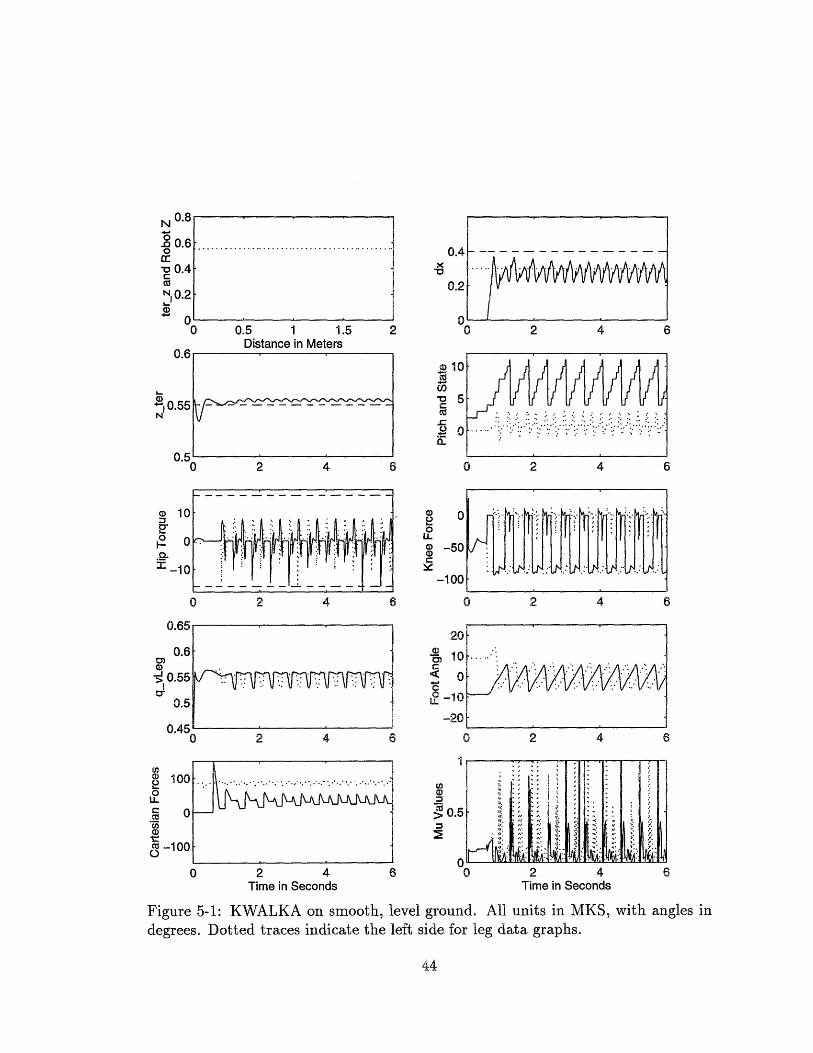
5-1 KWALKA on smooth, level ground. All units in MKS, with angles

in degrees. Dotted traces indicate the left side for leg data graphs. .. 44

5-2 KWALKB performance on smooth, level ground. All units in MKS,

with angles in degrees. Dotted traces indicate the left side for leg

data graphs. . . . . . . . . . . . . . . . . . . . ............. 47

5-3 KWALKA performance on rough, level ground. All units in MKS,


data graphs. . . . . . . . . . . . . . . . . . . . . . . . . ...... 49

5-4 KWALKB performance on rough, level ground. All units in MKS,


data graphs. . . . . . . . . . . . . . . . . . . . . . . . . ...... 50

5-5 KWALKA performance on very rough, level ground. All units in

MKS, with angles in degrees. Dotted traces indicate the left side for

leg data graphs. . .................. .... 52

9

5-6 KWALKB performance on very rough, level ground. All units in


leg data graphs. . . . . . . . . . . . . . . . . ....... 53

5-7 KWALKA performance on a smooth, uphill slope. All units in MKS,


data graphs. . . . . . . . . . . . . . . . . . . . .. 55

5-8 KWALKB performance on a smooth, uphill slope. All units in MKS,


data graphs. .................. 56

5-9 KWALKA performance on a smooth, downhill slope. All units in


leg data graphs ............................... 58

10

Chapter 1

Introduction

1.1 Why Legs?

Although the wheel was invented thousands of years ago, scientists, inventors, sci-

ence fiction writers, and dreamers have been contemplating legged locomotion for

at least hundreds of years. Legs are attractive for numerous reasons. A vehicle

or robot that walks instead of rolls has distinct advantages over uneven terrain.

An active suspension is inherently a part of a legged system, allowing large scale

control of body height and attitude. Legs can handle larger discontinuities than

wheels or even treads. Finally, some motivation comes from a desire to make robots

that more closely resemble their human inventors. Robots could then interact with

people more like people interact with each other. Although legs are an arguably

superior form of locomotion, wheels are found nearly everywhere today while legs

are found principally on toys and temperamental robots in a few research facilities.

The reason is that wheeled systems are much easier to control, power, and main-

tain, given today's technology. Self contained legged systems still suffer from severe

limitations in speed, balance capability, sensing, and power density. Research in all

of these areas promises to continue this slow walk towards reality for this dreamy

mode of movement.

11

1.2 Why Blind?

While arbitrarily detailed information about the terrain can be provided to the robot

in simulations, actual implementations limit the precision to which this information

can be known. For this reason, minimizing the knowledge of upcoming terrain in the

simulation eases the algorithm's implementation on a physical system. In the limit,

forward sensors are eliminated altogether, and the robot walks blind. This removes

a large amount of computation from the walking control. It also means that vision

or ranging could be used for a higher level, low frequency path planning to guide

the general direction of the walking, so as to avoid rises and drop-offs which are too

steep to handle.

1.3 Why Bipedal?

Implementing such a system on a bipedal robot seemed to focus the issues most con-

cisely. Since this model has point feet, no torque can be exerted on the ground. This

means the gait is only statically stable in the double support phase. As roughly 10

percent of the time is spent in double support, dynamic stability becomes an issue.

The controller has to run fast enough to stay ahead of the tipping time. The max-

imum joint torques and/or forces become a limiting factor, although computation

time is limited at the same time. The option of stopping to think was not allowed,

making for a reactive algorithm which does its best with the conditions in which

it finds itself. This requires an approach which performs a reasonable number of

calculations and exercises loose control over the robot's inherent behavior. It must

remain sufficiently flexible to accommodate what lies ahead.

1.4 The Approach

The algorithm developed in this work uses information from the robot's current

state-horizontal velocity, joint positions, and ground contact-to determine control

12

outputs. It was first implemented on a model with revolute hips and prismatic knees.

Then calculation functions to transform the inputs and outputs of the controller for

a robot with revolute knees were added. This adapted the algorithm for use on a

second model, which is representative of an existing physical robot. Parameters were

tuned to smooth vertical oscillation, minimize horizontal acceleration, and handle

maximally steep positive and negative slopes.

13

Chapter 2

Background

2.1 A Brief History

Countless attempts at walking, running, hopping, or crawling machines have been

made in the past few centuries-some successful, some not so successful. Concepts

have been based on novel mathematical relationships, elaborate mechanical devices,

and observations of people and animals. Creations have ranged from mechanical

horses and bugs to computer controlled pogo-sticks and man-amplifier suits. While

purely mechanical systems typically stumble because they cannot adapt to changes

in the terrain, computer controlled systems still get bogged down with even moder-

ately uneven terrain. Sensor limitations and non-ideal actuators further complicate

the problems.

Recent work in legged locomotion is progressing in a handful of laboratories

around the world. Walking robots range from bipeds to hexapods [1] [3] [4], while

running and hopping robots have operated on one, two, and four legs [8]. The study

of legged locomotion in animals, humans, and in simulations is more wide-spread [5]

[6]. Applications range from medicine and optimizing human athletic performance

to computer animation and actually building legged robots [5] [7] [9].

15

2.2 A Summary of Rough Terrain Work

Most rough terrain work has been based around four and six legged walking plat-

forms [4] or general running systems [2] [9]. The primary issue in this work is foot

placement: both choosing where to put each foot on the ground and how to load

it after contact. Primary problems include terrain detection, path planning, and

actuator power. Vision systems are beginning to develop the processing required

to pick out relevant features in video data, and sufficient path planning algorithms

have been worked out. However, these issues and the actuator limitations still limit

most of this work to simulations.

In a simulated world, these problems can be solved by assumption. Arbitrarily

detailed knowledge of the environment and the robot can be provided for free, power

density and actuator speed can be increased as required, and arbitrary computing

power can be dedicated to the simulation. The constraint of time need not even exist,

as frames can be rendered slowly and played back at a faster rate. Simulation has

allowed research to continue beyond the barriers still standing in the path of physical

system development. Once real systems catch up with simulation assumptions, the

knowledge gained from simulated systems should speed further development.

2.3 Biped Walking on Rough Terrain

While some biped walking algorithms have been implemented with varying levels

of success and robustness, any rough terrain attempts on two legs have presumably

involved adapting smooth terrain algorithms to deal with irregularities in the sur-

face. Many attempts seem to be an afterthought based on an initial smooth terrain

algorithm's success. The work in M.I.T.'s Leg Lab has always assumed smooth

terrain in actual implementations. Knowledge of when the flight phase will end is

quite important for their robots. This requires knowledge of what lies ahead, which

can be provided by sensing systems or fulfilled assumptions.

16

Some papers from this lab deal with rough terrain but assume that the terrain

is known in advance. While these approaches will be useful once sensing technology

catches up, they provide little beyond interesting thought and simulations for now.

The inverted pendulum walker demonstrates the closest approach to rough ter-

rain preparation from the onset [3]. Since the motion is using force control to keep

the body at a constant height above the ground, uneven terrain becomes a perturba-

tion to the leg length. This observation led me to develop an biped controller which

tried to keep the body at a constant height. I expected rather robust results from

this if two major precautions were taken to avoid detrimental interaction with the

ground. The first is to lift the feet high enough to clear what terrain may be under

the swing leg. The second is to return the swing leg to the uncertain ground level

without slamming it down. Once these problems are solved, quite extreme terrain

became easily passable.

17

Chapter 3

The Models

3.1 Overview

This simulation models a planar bipedal robot walking on rough terrain. Roll,

yaw, and lateral movement are prevented by a planar training joint attached to the

ground. This connection only allows for translation in the XZ plane and pitching

about the Y axis. The robot's knowledge of the terrain is based solely on information

available from foot contact. The terrain consists of an XY grid of points with

specified elevations, connected by planar patches. The model parameters are set

to approximate an actual biped robot being developed in this lab. Actuator force

limits and robot mass properties model those of the actual robot.

3.2 The Ground

Interactions with the ground model a collision with a pre-loaded linear spring

damper. To speed computation the simulation only checks for contact at the user

specified points of the robot. This can lead to entertaining crashes when the robot

falls through the floor and hangs from it's feet, but that non-reality is not an issue

unless things go dramatically wrong.

When a specified contact point lands on the ground, four spring damper systems

19

act on it. Spring constants, damping and pre-loads can be set for the X, Y, Z, and

0 directions. These values must be tuned for each robot until feet land without

bouncing and do not excessively penetrate the ground.

A rough terrain addition to this ground model was provided by Peter Dilworth,

a staff member in the M.I.T. Leg Lab. The model takes in a terrain file that allows

one to specify how high the ground is at a grid of points in the XY plane. A

new ground contact function linearly interpolates in two dimensions between the

specified points to produce a three dimensional terrain. Although arbitrary heights

can be specified at any point on the XY plane, the work discussed here kept the

terrain linear. Heights only changed with movement in the X direction. The robot

is limited to move in two dimensions, but it is still a three dimensional structure.

Varying the terrain with Y would make the robot walk along a hillside, effectively,

since the left and right legs are separated in the Y direction. I have left this as a

future expansion of this work.

3.2.1 Ground Variables

While interactions with the terrain are handled internally, it is nice to see what the

robot is doing, and it is necessary to know how far off the ground the robot is. Having

access to the terrain variables allows the control system to easily calculate the body

height, and it makes it possible to graph the terrain. The following variables are

shown in Figures 3-1 and 3-2:

q.z The vertical hip position relative to original ground level. This value is provided

by the simulator. However, if more realistic issues such as robustness to sensor

noise are important, this data should not be used. Instead the height to the

ground should be calculated through a leg which is in contact with it.

termz The height of the terrain above the original ground. This is updated each

control cycle to give the height of the terrain directly under the body. No

state directly uses this information, but it is useful for displaying the robot's

20

view of the terrain it walked over.

z_ter The position of the hips relative to the terrain. This is the difference between

q.z and ter z and serves as the robot's measure of body height. A PD controller

modifies the desired vertical force on the body to control this height.

3.3 KWALKA

My first approach, referred to as KWALKA, employs revolute hips on the bottom

of a block body with prismatic knees. This allowed speedy initial development of

a walking algorithm with intent to modify it for uneven ground. Initial work was

easier with the prismatic joints for a number of reasons. Problems were more easily

diagnosed and offered more intuitive solutions than a system with a revolute joint

at each location. The whole structure was easy to directly analyze and tune. The

variables measuring joint positions were easily understood, so images of desired

behavior were easily quantified and geometric constraints and actuator limits were

simple to choose.

Once the high level control had reached stability on level ground, adaptation

to uneven ground proved rather trivial. This is perhaps a result of the force-based

control when dealing with the ground. Changes required to deal with rough terrain

involved checks to guarantee ground clearance on the swing foot, and handle situ-

ations when feet hit the ground unexpectedly. Uphill grades favored shorter stride

lengths, while downhill sections were best handled with longer steps. Further work

improved the efficiency and reduced peak actuator forces and torques.

The peak actuator output required was of primary concern in developing a real-

istic simulation. A robot with an enormous power to weight ratio has little trouble

dealing with hills and moving its limbs quickly enough to maintain very high veloc-

ities, but real mobile robots have real limits which force the development of more

efficient approaches. The key to keeping the simulation realistic was keeping the

peak actuator output below the limits on the physical robot. For the hip joints,

21

this is easily checked. With prismatic knees, however, a constant force limit is not

sufficient when trying to emulate a robot with revolute knees. The peak longitu-

dinal force a revolute knee can produce is a function of the knee bend. While a

peak longitudinal force could be calculated based on imaginary knee bend, the most

direct way to emulate the real robot is to reconfigure the simulation.

One may ask why the robot was not built with prismatic knees, if these are sim-

pler to conceptualize. Prismatic joints are usually avoided for reasons of complexity

and durability of actual implementation. Additional material is required to prevent

binding, and the drive system is continually subject to any forces on the leg. Since

the power to weight ratio is a primary limitation for mobile robots, designs which

require additional material to perform a given task are not preferred. Reliability

and mean time between failures is a second issue. Having more parts which are

pushed closer to their limits has a detrimental influence on the run time to repair

ratio, making a real robot very time consuming to maintain.

3.3.1 KWALKA Variables

The configuration variables of KWALKA are shown in Figure 3-1.

q.pitch Measures the body rotation from vertical, with nose towards the ground

being positive. On a real planar system, this is easily sensed from the planar

joint rotation. On a free robot, deviation from vertical would have to be

measured with some sort of gyroscope, camera system, or vertical range-finder.

Obtaining this data is not trivial, but it is not exceedingly difficult. It is very

important information to have.

q.rhip Measures rotation of the hip relative to the body. Rotation under and

towards the rear marks the positive direction. This data is readily available

from a potentiometer or shaft encoder on a real system.

q.rknee Measures displacement along the leg axis. Upward motion is positive,

and full extension is the zero point. This is effectively a measure of shank

22

Figure 3-1: Configuration Variables of KWALKA

23

retraction. A variety of linear position sensors could provide this input on a

real robot, such as linear pots or magnetic coils,

q.z The distance from the hip to base ground. This is easily obtained on a two

dimensional robot, as the vertical motion of the support can be measured;

however, one of two different methods would be required on a free robot:

Either calculate the ground height through the knee and hip parameters when

a foot is on the ground, or add some sort of altimeter/range-finder to monitor

the ground height below the body. Precision requirements may force one to

use the more complicated method.

q.x The distance from the hip projection on the X axis to the global origin. This

simply keeps track of how far the robot has traveled, but it's derivative is very

important for the gait control algorithm. With a boom or treadmill, this is

straight forward data to obtain. However, two integrations of inertial data is

one of the few ways to measure this in a free robot, and that makes noise a

key issue. The algorithm has no need to accurately know the X position, so a

real implementation could approximate step lengths if the data were deemed

useful. The terrain needs this information, however, and it also allows the

simulator view to track the robot as with walks.

qd.x The velocity along the X direction. This provides input for a first order veloc-

ity control in the double support phases. It also is important as a condition

to end double support. Once the velocity is sufficient to coast over the lead

foot, the trailing leg must enter the swing phase in order to be in place soon

enough to prevent a fall.

thetar The angle of the hip relative to vertical. This value increases as the hip

swings down and to the rear. It is simply calculated from the global body

angle and the angle between the thigh and the body. Position controlling the

supporting hip to this value keeps the body near level.

24

3.4 KWALKB

In order to prove sufficient efficiency, the algorithm was implemented on a second

model, known as kwalkb. This model has revolute hips and knees, with the approx-

imate geometry, mass properties, and actuator limitations of the physical robot. It

required transformations on both sides of the control system to express the actual

joint data in terms that the controller understood and to map the controller's com-

mands onto the joints. This is a required step for implementation on the actual

robot, as well, so it was work necessary at some point. While the controller still

operates on a virtual prismatic leg, the actuator limits now correspond directly to

those of the actual robot. Now physically achievable performance is easy to verify.

Also, when the controller requests too much torque, motor saturation is now

simulated. The maximum torque is provided is fixed, placing a constraint on the

maximum virtual leg force which varies with knee bend.

3.4.1 KWALKB Variables

In addition to its configuration variables, KWALKB needs to calculate the data

that the virtual leg would provide. All the variables are pictured in Figure 3-2. Only

the right side variables are listed, since the same description is true for the left side

as well. The physical variables are as follows:

q.pitch Measures body rotation relative to vertical, as on KWALKA.

q.rhip Measures rotation of the hip relative to the body. Rotation under and

towards the rear marks the positive direction. This data is readily available

from a potentiometer or shaft encoder on a real system.

thetar The angle between the thigh and vertical. This is the same on KWALKA.

q.rknee The outside angle between an extension of the thigh and the shank. This

is the angle which fixes the distance between the hip and the foot. As with

q.rhip, this is easily measured with a rotary sensor.

25

q.pitch

theta_r

" A1

sitiveleta

e

Figure 3-2: Configuration and Virtual Variables of KWALKB

26

xI

q.z Hip height from ground zero. This is the same as for KWALKA.

From these physical values, the controller can compute the data that a prismatic

leg would be returning if its end points coincided with those of the real leg. The

virtual data is put in the following variables:

qsrfoota The angle a line connecting the hip to the foot makes from the vertical.

From the physical variables, alpha and beta, the upper and obtuse angles in

the real leg/virtual leg triangle can be found. These provide an intermediate

step to calculate the angle of the virtual leg with respect to vertical using the

law of cosines.

qrvleg The distance between the hip and the foot. This is the length of the virtual

leg. Again, the law of cosines can be used to express this length in terms of

alpha and the link lengths.

3.5 Servos

In both models, a variety of servos can drive each joint. The default option is a limp

servo, which exerts no torque at the joint. The planar joint employs limp servos

along the X, Z, and pitch axes. In some states, other robot joint servos are set to

be limp to keep foot contacts from generating contending shear forces.

A position control servo uses proportional and derivative gains to control the

angle or extension of the joint. This mode is used to put the robot in the initial

configuration. Once walking begins, position control is used to move the swing

leg and to control the body pitch. The proportional term is closely related to the

maximum forces, so the program takes this parameter from the user. In order to

achieve the desired damping characteristics, the user specifies a damping ratio, from

which a function calculates the required derivative gain.

A third type of servo available is PD position control with a feed forward force or

torque term. This mode uses the same gains as the PD mode, but adds the ability

27

to directly add output torque of force to the PD control. This can shrink the steady

state errors when approximate forces can be calculated. The PD control can then

correct for errors between the requirements and the estimates, achieving the same

total errors with lower PD gains, and therefore, better stability.

A pure feed forward servo is a fourth option. This ignores the position and

derivative terms entirely and exerts the commanded force or torque, regardless of

where the output is or how it responds.

A final mode is the feed forward servo with damping. The commanded force or

torque is applied, but a viscous friction term generates a resistive force proportional

to the velocity. This generates a constant velocity servo, which is used to lower the

feet to the ground.

Servo outputs are constrained to reasonable limits on KWALKA and to the

limits on the actual robot on KWALKB. For KWALKB, this ensures both that

controls within the simulator will not exceed the maxima of the real robot and that

the simulation's behavior will also predict performance degradation as situational

demands exceed the actuators' abilities. Left unchecked, the actuator outputs could

be recorded and screened to verify that maxima were not exceeded, but this would

not demonstrate what may happen if the real robot is subject to situations which

demand greater torques than the motors can provide.

28

Chapter 4

The High Level Control

4.1 The Basic Control System

The control system is a finite state machine which cycles through a series of states

corresponding to each phase of the walking gait. While entering each state, the

joint servos are put into a desired mode. One or more conditions specify when

to transition to another state. While these conditions are not met, the joints are

controlled as directed by the current state. The controller for both models operates

on the distance from the hip to the foot and the angle between vertical and the hip

to foot line. This in effect assumes that both models have a revolute hip with a

prismatic knee.

For kwalka, this is the arrangement, but for kwalkb, this is a virtual structure.

The commands for this virtual leg and the data about it must be transformed to

deal with the leg that is actually there. This high level controller computes desired

Cartesian forces which are then transformed to desired joint torques or forces. The

desired vertical force is computed by a proportional plus derivative controller. It

commands a vertical force to maintain the body height at the nominal Z parameter

in all states. In single support mode, the only direction of force possible is in the

line of the virtual leg. This fixes the ratio of the vertical to horizontal forces, so

only one Cartesian force can be controlled in single support mode. By setting the

29

desired vertical force, body height is controlled, while forward velocity is left to do

as it will.

The desired horizontal force is calculated only when both feet are on the ground.

A simple proportional velocity controller works to maintain the horizontal velocity

at the set-point. The robot's forward velocity slows significantly as it moves over

the foot in single support, due to the constant height constraint. Once the body

has crossed the foot, it accelerates until the swing leg lands. This controller simply

applies a force proportional to the velocity error whenever possible (ie. in double

support phases). The maximum horizontal force varies with configuration, so the

force is limited at the joint level. When the controller commands too great a hori-

zontal force, a net upward force results on one of the feet. The controller assumes

that the ground is sticky and can therefore be pulled upon as well as pushed. This

behavior is prevented by checking the net force on a supporting foot due to the

joints. If this net force ever tries to pull on the ground, the joint commands are

adjusted to maintain a slight downward force on the ground.

4.2 Control Variables

Several variables affect the nature of the walking behavior.

qdd.x Desired X velocity. This parameter is the set point for a proportional

velocity controller. The controller uses the difference between this set point

and the actual Cartesian velocity to determine the desired horizontal force. In

the double support phases of the gait, the weight is distributed between the

feet to provide this force while supporting the robot as well.

q_d.z Desired hip height. This input is the set point for a PD controller that

calculates a desired Cartesian force to control the robot's height above the

ground.

30

theta-min Minimum forward angle to terminate the swing phase. This parameter

specifies how far forward the swing leg must rotate before the swing phase is

complete. This corresponds quite closely to stride length.

swinglead The offset used when the swing leg mirrors the support leg. This value

is added to the negated support leg angle in order to put the swing leg ahead

of being symmetric with the support leg. This allows better velocity control,

since the lead leg touches down farther ahead of the body. The widened stride

length allows a broader range of horizontal forces to be commanded.

gclearance A vertical offset for the swing leg. The swing foot must clear the last

ground contact point by this value before the foot is considered clear to swing.

swinghi A vertical offset that determines the desired swing leg height. The desired

value of the swing foot height is set from this offset, which is greater than the

g-clearance offset. This puts the leg in motion towards a higher point. The

clearance point provides a trigger to begin the swing, in anticipation of where

the foot will soon be.

swingh A vertical offset for the swing leg relative to the support leg. On uneven

terrain, the swing foot may leave the ground well below the support foot. If

the desired position obtained from the swing-hi offset is insufficient to clear

the height of the support foot, swing-h is used to find a new desired position

for the swing foot.

4.3 The States

The finite state machine's states include: initialization, stabilization, and re-

peated states for double support, double to single support transition, single sup-

port, and single to double support transition. Figure 4-1 summarizes the sequence

of states. The repeated states treat the left and right steps separately, so the state

31

State 0One-Time Initialization

State 1Startup Initialization

State 2Position Control

State 3Force Control

,i

State 5Transition to Single Support

on Right Leg

State 6Single Supporton Right Leg

•__••

H-

State 9Transition to Single Support

on Left Leg

State 10Single Supporton Left Leg

t

Figure 4-1: The Controller States

32

State 4Double Support

Right Leg ForwardI

State 8Double SupportLeft Leg Forward

State 7Transition to Double Support

Left Leg Forward

State 11Transition to Double Support

Right Leg Forward

I .

- I.

I

completely summarizes the phase and lead leg in the gait. This proved to be more

straight forward, although somewhat repetitive.

4.3.1 Before Checking the State

There are a few calculations which are the same for all states. Rather than repeat

these inside each state, they appear in adapt-control, which is called at the beginning

of the control loop, before the state is determined. Two of these items use the rough

terrain function to interpolate the current terrain height under the body, and update

both the altitude of the terrain and the body height relative to it. Although the

terrain altitude is not used in the control, it is useful to be able to graph the robot's

perception of the ground height over time. I also used the difference between the

ground height and the robot height from ground zero to fill the relative body height

field. This information can also be calculated from the joint positions, as long

as the feet are on the ground. I chose the absolute height differences because it

simplified the expressions. This absolute measure of body height would be difficult

to implement without very precise altimeters, it serves the same purpose as the

more direct method of calculating the height from joint angles. If the robot model

introduces noise in sensors and actuators, the joint angle calculation must be used

to be consistent with the model.

The adapt-control function also computes other information, useful to the con-

troller and to the observer. The angle and distance of each foot relative to the body

is updated here, as well as an estimate of the terrain slope and the coefficient of

friction each foot is experiencing against the ground. While some of this information

is not directly involved with the control, it is useful to have available when assessing

how realistic the simulation was.

33

4.3.2 Initialization and Oscillations

States zero through three perform a series of set up and waiting functions which

put the robot at rest before the walking algorithm begins. State zero performs all

the one-time initializations, setting constants from the header file parameters and

setting up the initial state. Setting globals to the #defined values seems redundant,

but this allows initial values to be kept in the header file, away from the tangle of

controller code. Making them globals allows them to be viewed and changed at any

time in the simulation. This is an advantage when searching for correct parameter

values to tune the behavior.

State one performs the detailed initialization and goes on to state two, which

updates the knee commands to follow any user changes in the desired z height. After

a brief delay, all joints are switched into force control mode, and the knee position

gains are reduced, since position control is only used to move the knees when they

are in the air from this point forward. The damping required to roughly achieve

the desired damping ratio at each joint is calculated for the new gains. Finally, the

desired Cartesian forces are calculated and then transformed into joint forces. This

state waits for a moment so that any oscillations in the force control can settle out.

Then walking can begin.

4.3.3 State 4: Double Support, Right Leg Forward

In the double support phase, Cartesian forces in X and Z are commanded. The

lead leg's hip is position controlled to stabilize body pitch, but only while the lead

foot is in contact with the ground. This check prevents hip torque from slamming

the foot down if it bounces. The body tends to pitch forward in the single support

phase as the swing leg is servo-ed forward. Thus, using the lead leg to correct this

increases the downward pressure on the lead foot, while the trailing foot would lose

contact pressure if that leg were trying to correct the positive pitch error. Therefore,

the trailing leg's hip remains limp to keep the trailing foot on the ground while

34

Figure 4-2: Double Support

preventing internal forces from horizontally loading the feet.

Both knees operate in feed forward mode throughout the double support phase.

Having set the hip torques as above allows feed forward forces or torques for the knees

to be calculated from the Cartesian force equations, completing the transformation

from desired Cartesian forces on the body to joint commands.

The trailing leg is vital to contribute horizontal velocity during the double sup-

port phase. Once sufficient velocity exists to coast over the support leg with a

specified minimum velocity, the trailing leg can be lifted. This condition is devel-

oped by integrating the horizontal force acting if the lead leg were to support the

weight of the robot and rotate from its current position to vertical. This is the

energy that will be subtracted from the current kinetic energy. Since the vertical

height is held constant, the kinetic energy at vertical will be the current kinetic

minus the work done by the lead leg.

This provides a predictor for the velocity at vertical if single support begins

35

immediately. Once this final velocity clears the minimum velocity parameter, the

trailing leg should enter the swing phase so that it can be in position to begin the

next double support phase before excessive velocity develops from having the single

support leg behind the body. This calculation does not factor in the deceleration

from driving the swing leg forward, so the actual minimum velocity dips below

the minimum velocity parameter. It is a sufficiently small error, however, that the

minimum parameter can be adjusted slightly higher to compensate.

Time spent in the double support phase can both accelerate or decelerate the

body to bring it back to the desired velocity, depending upon which leg contributes

more vertical force. As this happens, the minimum velocity condition becomes less

demanding because the lead leg continues to rotate towards vertical. Eventually

the minimum velocity condition should be satisfied, and control will switch to state

5. As a precaution, state five will take over if the support leg crosses vertical even

if the condition is not satisfied. This case is only useful for real time control. It

is likely to help the robot regain a stable gait if it has momentarily exceeded the

algorithm's maximum velocity. It is quicker to skip to the next state after a direct

comparison than to evaluate the minimum velocity expression first.

4.3.4 State 5: Double to Right Support Transition

The principle role of the double to single support transition is to lift the trailing leg

off the ground so that it may enter the swing phase and servo forward to prepare

for the next double support phase. The lead leg acts as if single support has begun.

The horizontal force is ignored in order to maintain the proper vertical force. The

body pitch is controlled by servoing the lead leg's hip, as in double support.

The trailing leg is servo-ed to raise the foot to a required ground clearance so

that it will not hit the ground in the swing phase. With the prismatic knees, only

the knee is position controlled to lift the foot and the hip is left limp. The revolute

knee version uses action from both the hip and the knee to lift the foot off the

ground along the angle of the virtual leg.

36

z

Figure 4-3: Transition to Single Support

The single support state is entered when the rear foot has been lifted higher

than the larger of the lead foot height or the minimum ground clearance and the

rear foot switch shows no ground contact.

4.3.5 State 6: Single Support on Right Leg

The single support phase simply rides out the transition of lead legs. The support

leg's knee is force controlled to maintain body height, while the hip is position

controlled to keep the body level. The swing leg is position controlled at both joints

to keep the foot above the last ground contact or above the supporting foot by the

ground clearance factor. The swing leg also positions the foot to mirror the angle

to the support foot, plus a lead factor. This smoothes the transition from trailing

leg to lead leg.

Once the swing leg reaches a minimum forward angle, the swing phase is com-

plete, and the transition to double support happens in state 7. If the swing foot hits

37

--

z

Figure 4-4: Single Support

the ground early, one of two actions is taken. If the swing leg is ahead of the support

leg, this simply means that the transition to double support has already occured.

The transition state is skipped, and the next double support phase is begun in state

8.

If the swing foot hits the ground while it is behind the support leg, a little

stumble is executedj by jumping back to state 4. A severe toe-stub can remove

sufficient energy to make it impossible to maintain vertical height and rotate over

the support foot. By returning to the double support phase, the controller can try

ensure there is sufficient energy to coast across the support leg. If the foot hits too

far forward of the body, the is no chance to inject additional energy. A backwards

fall is then unavoidable without quickly repositioning the feet.

38

z

- -

zz

X X

Figure 4-5: Transition to Double Support

4.3.6 State 7: Right to Double Support Transition

This state is responsible for putting the swing leg back on the ground. This issue

is somewhat complicated because the ground elevation beneath the lead foot is not

known. To surmount this lacking information, a constant rate of descent is used to

lower the foot until it hits the ground. The rate is chosen to be as quick as possible

without excessive bouncing, and is set by the combination of a feed forward force

and a damping constant. Once the foot registers ground contact, the next double

support phase begins.

4.3.7 State 8: Double Support, Left Leg Forward

This state repeats the calculations of state 4, but with the left and right roles ex-

changed. The left hip now controls the body angle while the right hip remains limp.

More speed is provided by biasing the weight to the right foot, while deceleration is

39

caused by biasing to the left foot. The energy calculation triggers the transition to

state 9.

4.3.8 State 9: Double to Left Support Transition

While the right hip remains limp, the right foot is lifted from the ground. Once

it sufficiently clears the ground or the left foot, single support on the left leg is

controlled in state 10.

4.3.9 State 10: Single Support on Left Leg

Single support is executed on the left leg, simply mirroring the conditions and

controls from the right leg support. The state can switch to 11 if the swing leg

reaches the minimum swing angle, to 4 if the foot hits the ground in front of the

support foot, or to 8 if it hits behind.

4.3.10 State 11: Left to Double Support Transition

As before with the right to double support transition, the swing foot is lowered to

the ground, and double support in state 4 begins once contact is made.

40

Chapter 5

Results and Observations

The final performance of both models was quite surprising. Once the algorithms

performed on smooth, flat terrain, bumps and significant hills required little more

than tuning some parameters. A few new state transition conditions were added to

remedy failings which were due to improper state assignment. These new conditions

included issues like choosing which state to enter after single support if the swing foot

hits the ground before reaching its goal angle. A few bugs in condition calculations

even crept out towards the end when an improper variable was used in place of one

that measured a similar, but different, value.

For this discussion I will divide the terrain into three main types: terrain with no

net slope, terrain with a net up component, and terrain with a net down component.

Each type can be smooth or rough to varying degrees. Data is shown from smooth,

rough, and very rough versions of level terrain and smooth slopes. The up and

down slopes represent the maximum steepness for which I could tune the individual

models.

In general, the desired X velocity is kept low on all terrains. This always keeps

the maximum forces lower, and it also keeps descents under better control. The

double support phase attempts to prevent the velocity from ever falling below the

minimum specified, but its prediction of the velocity after lifting the rear leg is

based only on the robot's mass and the action of the support leg. There is a rather

41

significant reaction to the swing leg motion which makes the actual velocity in the

swing phase drop lower than anticipated. The .3 m/s minimum I used in all cases

proved adequate to prevent a backwards fall, but it was more like specifying the

average velocity than the minimum.

5.1 Level Terrain

On level terrain, step length can be kept at a moderate size and the ground clearance

variables are kept small. Short steps make for the most efficient motion, since the

support leg must do little more than maintain its length, but the robot must then

cope with more interactions with the uncertain terrain. If the step is too short,

the robot can easily be upset by a drop in terrain, since that results in additional

forward velocity that must be controlled by biasing weight to the lead leg in double

support. If the lead leg is not sufficiently far ahead, the velocity cannot be reduced

to the desired level. After a few steps this velocity can build out of control until

the swing leg can no longer reach a position in front of the robot before it hits the

ground.

If the lead leg swings too far forward, a down hill slope causes a fall. The leg

cannot reach the ground after the swing phase, and the robot has to leave the leg

extended and wait to fall onto it. This is usually catastrophic.

Keeping the swing leg close to the ground helps smooth out the transitions into

and out of double support. This reduces the delay between the decision to pick up

or put down a foot and the completion of the action. The conditions for lifting or

putting down a foot neglect the transit time. At significant swing heights, this can

become a significant factor in the ability to control the velocity.

An additional set of factors with great significance for the stability of the gait

is the swinglead and theta-min combination. If the swing lead is too large, the

steps become very long. To accommodate long steps requires additional power or

significant body bounce. When the lead is too small, the swing leg gets behind,

42

and the velocity goes out of control. Thetanin couples with swinglead to find

a balance between the control of the velocity and the efficiency. While no direct

efficiency is calculated, the maximum torques and forces available from the joints

prevent grossly inefficient gaits from being stable for long.

5.1.1 Smooth Surface Performance

Performance on smooth terrain was very good, but it did seem to suffer from the

precautions present for handling rough terrain. Figure 5-1 presents the data sum-

marizing the behavior of KWALKA on smooth, level terrain. The body exhibits

small oscillations just above the set point. These are due to the simple PD height

controller. It reacts to deviations caused from imperfect knee forces and commands

more or less total vertical force to correct for deviations from the set-point.

The positive steady state error is due to an over estimate in the approximation

used in calculating the force due to gravity. The thigh masses are being supported

by the knee joints, but usually at an angle off vertical. Therefore, the linear joint

structure is bearing some of the load, and the knees would not have to bear the

entire weight. The calculations treat the force due to gravity as a constant and set

the knee forces to counter it at all times.

The horizontal velocity exhibits oscillatory behavior for an unavoidable reason.

The system is under actuated in single support. The vertical position control is

given pressidence over the horizontal velocity, so each swing phase was expected to

cause the velocity to fall and rise again. With no terrain disturbances and the small

step length this run used, the double support states do not last long enough for the

robot to achieve the desired horizontal velocity. Then, the velocity dips below the

set minimum value because of the neglected swing leg interaction. This actual lower

bound is a function of the swing leg mass properties and the forces applied to it.

Since this is a constant offset, the minimum velocity set-point must be high enough

to accommodate this loss.

The plot of the state shows the initial phases leading into the cycle of gait states.

43

0.5 1 1.5 2Distance in Meters

2 4 6

0 2 4 6

V. a0 2 4

0 2 4Time in Seconds

0a)0

LL

0aYe

0 2 4

20

T5 10

< 0-o

-20

6

1

Cl)

0.:3>0 O. ,2

f

6

6

0 2 4

I : : ! t[ i:i' ' I� i 1 i i i 1,,bP.I,;'· i% G " f% s* �· ·-- � -·�.. 5 r ·d,· ,·

h· r.' r\:I r·· r.· � )

U-0 2 4

Time in Seconds6

Figure 5-1: KWALKA on smooth, level ground. All units in MKS, with angles indegrees. Dotted traces indicate the left side for leg data graphs.

44

0.4x'a

N 'U,

n 0.60

-o 0.4C(U

N 0.2~.1(D 1

V

0

a 0.55N

0

0. 2

A0 2

10(U

05C

coQ.-Y?

4

4

1

-1

6

6

.. .... ·' ·.·

a)

0I -.:

0 2

U.00

0.60)

> 0.55

0.5

VVV\V\FWW\V\F\F~V

0U.0

LLC

O(Uo

.... ffifimm �

·

Jr i4lt.A:·A64MWM1.1 ·IU. N

I

I

U.A)

- -- - - - - - - - - - - - - -·

V�

,,· · ·U%

I

a* �s

" '

· �n· rr · · II.- la ·. II · � ·

·· Ir ·�

i

Each drop of the state from 11 to 4 represents two steps. In this trial, the double

support periods account for nearly half of the cycle time. Over half of the remaining

time is spent in the single support phases. The short stride length and low ground

clearances used here make the transitions between support modes very short.

In order to obtain sufficient joint velocities, the joint damping had to be kept

quite low. This results in pitch oscillations in response to the swing leg movements,

which remain bounded between plus and minus 3 degrees.

The hip torques remain between the bounds, except for a single spike at the

onset of a right foot swing phase. The hip torques are limited by clipping desired

position commanded to keep the hip response within the torque limits. This does

not account for the derivative term in the controller, which provide an opportunity

for the hip torque to momentarily exceed the defined maximum limit. Adding the

derivative term should keep the limits more strictly enforced. Since the knee forces

are directly commanded, they are kept strictly within the defined limits. The forces

are quite biased in the downward direction, which may make designs which take

advantage of this more efficient. A symmetric drive costs additional weight for force

potential in directions that are not used.

The parameters tracking the virtual leg-in this case, the actual leg-are also

shown. The small deviations in leg length and small motions of the feet summarize

this gait's small power expense.

The Cartesian forces act as expected. The vertical force hovers about the weight

of the robot. Small deviations in vertical height require only minor adjustments

in this direction. The horizontal forces peak at the onset of each double support

state. This indicates that significant velocity is being lost in the swing phase each

time. The magnitude decreases to a steady state level after the first few steps. A

larger gain on the velocity controller could reduce the steady state error, but the

step length is a primary limitation on the settling time.

The final plot displays the effective coefficients of friction for the left and right

feet. It goes to zero when the foot is off the ground. This is monitored by the

45

foot switch variable for each foot. The forces seem to dissipate out of proportion,

however, and a delay in registering foot separation from the ground causes spikes

each time a foot is lifted. Without the spikes, this gait requires a friction coefficient

of at least .2.

The results for KWALKB on smooth, level ground are shown in Figure 5-2.

Better control of the swing leg angle gave this run a longer stride length. This

improved the horizontal velocity control but degraded the vertical stabilization.

The velocity control was nearly perfect, with the range only slightly exceeding the

desired max and min settings. This is likely due to the slightly lower body height

than desired. The anticipated loss of energy is not as great as actual, so the disparity

between the actual minimum and the desired minimum goes away.

The torque limits on the knees cause a more stringent limitation on the maximum

virtual leg force that becomes worse with knee flexion: The more the knee bends,

the less force the virtual leg can produce. The stride length limits the body height

set point, since the feet must reach the ground at the limits of the step. This forces

the knees to operate at a large enough flexion to make the virtual leg much weaker

than on the prismatic model.

The Cartesian forces also show greater variation due to the wider stance. While

the vertical force changes significantly, the desired horizontal force eventually shows

only small spikes to restore energy lost in the step. While the desired horizontal

forces are smaller, the applied forces are larger because of the wider stance. This

drives the required coefficient of friction up to at least .4 at the start.

5.1.2 Rough, Level Terrain

The next set of tests were run on a randomly generated terrain spanning a list of

points 0, 1, 2, 3, and 4 cm high. This required additional swing heights and swing

leads to prevent tripping or stubbing the feet on the bumps.

KWALKA showed significantly larger altitude variations on this terrain. The

terrain changed faster than the altitude controller could respond since each step put

46

0 0.5 1 1.Distance in Meters

V.0.

0

0

2

2

4

4

5 2

0.4x'a

0.2

0

10

5

0CL

6

6

0 2 4 (

0

0e

0

a)

2 4

0 2 4

6

6

20

*- 10

0,o -10

-20

2 4

2 4 6Time in Seconds

1

ci,

>00.52O~

nC

i...h

M

z

A' A .A . .J A

2 4Time in Seconds

J,.,,, I A AkJ J \6

Figure 5-2: KWALKB performance on smooth, level ground. All units in MKS,with angles in degrees. Dotted traces indicate the left side for leg data graphs.

47

N ',

0, 0.60rr-a 0.4

N1 02

0A

V.U

A}0.55N

I. J

_V f___vvv\___ v

10

0

0

-

-10

(0)0.. I>1

0.6

0.55

0.5

V..tij

0 2 4

. , ..

08 100( o

LOC _

0

o -1000

0

6

. : I . : . - : - - . : '. . 'I : : .,

:·· - - - - - -

F"I\

·

. `'"'"" LiY-L.- · · ... .. . .... .... A..,

I

nA11M

I

m

I

.

AjI _.,B

vV0.1

- AP" '

6 O

I)

·

·

A- ' ;'

the foot at an unpredictable new height. The longer stride length kept the velocity

under control, despite the sudden drops encountered in the terrain. The velocity

regularly dips lower than it did on smooth terrain, but each double support phase

manages to restore it to the set-point.

Double support takes up a longer segment of the stride cycle because the lead

foot lands farther ahead. The pitch oscillations oscillate with the same magnitude,

but are now biased slightly negative. Hip and knee torques are more widely varied

than they were on smooth ground, but the average magnitudes only increase slightly.

What changes significantly is the range of leg lengths. This is due in part to the

longer stride length. The uneven ground causes additional modulation, making for

marked increases in the motion of the legs. This test demanded much greater energy

output from the robot.

Other new features this behavior exhibits are the zeroing of the desired horizontal

force and the oscillation evident as the legs swing forward to -10 degrees. The longer

strides cause both of these features to appear. The required friction has grown from

the smooth ground case as well. There are fewer extraneous spikes, but the valid

sections are higher.

Figure 5-4 shows the results of sending KWALKB across the rough terrain.

Comparison with the smooth terrain test shows an increase in altitude variation,

although it is always below the set-point. The gait cycles become less regular, and

some of the double support phases lengthen considerably. The velocity remains

very well controlled, with a slight variation beyond the bounds after a significant

bump. Hip torques actually drop, and knee torques remain about the same. The

last step with the right foot lands hard, as can be seen from the larger knee torque

commanded at that point.

The range of virtual leg lengths and angles expands dramatically. This is mostly

due to the lead leg taking a long time to come down when stepping into a depression,

because the foot continues to move forward as it descends. The friction demands

increase rather dramatically as well.

48

N Vt0.a 0.60n:· ' 0.4CUN 0.2

10)

0 0.5 1 1.5Distance in Meters

0 2 4

x'O

0.4

0.2

00 2 4 E

10

o 5C

_ 0a.

6 0

a)10(D

20tU-

0 2 4 6

2 4 6

0 2 4 6

2 4 (

2 4Time in Seconds

6

' 10C< 00t -10

-20

1

! 0.5

0

0 2 4 E

iMTime in Seconds

60

Figure 5-3: KWALKA performance on rough, level ground. All units in MKS, withangles in degrees. Dotted traces indicate the left side for leg data graphs.

49

1

'~ 0.55N

0.

a0> 0.550"

0.6

0.5

20

00.45

a, 100

-1000C lo

0

r ~ r~~~~~~~~~~~~

I -~_ - ;r _ _

I .

, . . ~ ~ ~ ~ ~ ~

.F

* _ I %~~~~~~~~~~~~~~~~~.

.·· ...... ·.. ·....'· �' · · �·-"·��·' · �··._·:····1.-···.·

'··' - '· ''

A. , _ , ._ . .~-

, , _

. _ .

w _ I

·.... ,........ c.:...... ..

a\ 1

2 6

0.6

r

rr PA

U.0:

6 I6

2 4

....

" ''

'

'

'''".. ·· rl ·..

.I· .· · ul I ·· · · v� r .·. - vr r · · ·vl r · ·.·

1 1.5 2Distance in Meters

4

4

4

x-o

V

0 2 4

1 0

C.

0

6 0

20

0

2 o0 C -10

-20

6

6

0

0

2 4

2 4

2 4

2 4Time in Seconds

c)co

2

:3

:E

6

1

0.5

00 2 4

Time in Seconds

Figure 5-4: KWALKB performance on rough, level ground. All units in MKS, withangles in degrees. Dotted traces indicate the left side for leg data graphs.

50

N u.

. 0.6

-O.4co0.4N1 0.21-1(D

V

0 0.5

0.t

N0.55

0

00

0.I

10

0

-10

I

0

2

2

2

6

6

6

6

0.65

0.60)

- 0.55

0.5

nfl A0

100,o

" 0

Co -100C)

0 6

hi · ·

" '·'' ·' '·'" ·- · · ·'' :. ·'· " ''�·. ... .·

·'··r

·

..

~~~~~~ .~~~~~~~~

-I·.·~ ' -.W. A... I.-N -~~~~~·

o..

....... I I......... ·

n

A.v

In L

I

Comparison of the two models on the rough terrain shows considerably less ve-

locity and pitch deviation in KWALKB. The hip torques are lower, and the height

varies by about the same amplitude. The revolute knee model shows greater varia-

tion of leg length and angle, however. This can cost additional energy. The efficiency

comparison is somewhat clouded by the greater hip torque in the prismatic model,

though. KWALKB's steps are longer and the average desired horizontal force is

much lower. It does demand greater friction, however.

The next piece of terrain doubled all the heights of the rough terrain to produce

very rough terrain. The grid points defining the terrain are 0, 2, 4, and 8 cm above

the floor. KWALKA shows similar changes to those between the smooth and rough

tests. The only notable increase is on body height control. The friction requirements

grow noticeably as well. The commanded knee forces are slightly larger, and the

virtual leg lengths and angles also increase by a small percentage. Figure 5-5 shows

summarizes the results.

KWALKB shows a much more dramatic difference between its rough and very

rough terrain performances. The vertical position error is much greater on the very

rough terrain, and the knee torque increases enough to saturate on the last right

foot step. The added vertical deviation aggravates the leverage disadvantage the

knees experience. The velocity swings up by more than 40 percent stepping off a

bump at the end.

Compared to the performance of KWALKA, the minimum velocity is better

regulated, but the maximum velocity is less controlled. The vertical deviations are

greater and still centered below the set-point. Hip torques are still significantly

smaller, but virtual leg motion is considerably larger. More friction is required.

51


0 2 4

0.4

0.2

11L

U)

'a

0F-J.mQ.s

10

5

0

0 2 4 6

0

0U)C)0U-

CN-

0

-50

-100

6 0

2 4

2 4

6

6

20

o10

0o -10

-20

02 4 6

2 4Time in Seconds

W

:3(I

6

2 4

Time in Seconds

Figure 5-5: KWALKA performance on very rough, level ground. All units in MKS,with angles in degrees. Dotted traces indicate the left side for leg data graphs.

52

N

,' 0.60-c 0.4

0.2

,IG)

v0

U)4I CN

aD

I-

, :.. :.. .I : . :

0.65

0.6a)j 0.55

0.5

n A-

0

I 1000

C " 0C)

CO -10000

6

f | . . .~~~~~~ . .~~~~~~

B . .

n.w

I.. . . . . ... . ... ...

n II

. . I

''·· · · ·. ·. ·:

6

0 0.5 1 1.5 2Distance in Meters

0 2 4

0 2 4

0 1

'2.

0"C

0 2 46

6

20

10

-C -10

-20

0 2 4

0 2 4,a

o0

.-

1=o

0

Figure 5-6:with angles

Co

~!0.55"o2

2 4 6 " 0 2 4 6Time in Seconds Time in Seconds

KWALKB performance on very rough, level ground. All units in MKS,in degrees. Dotted traces indicate the left side for leg data graphs.

53

N '-

0.60a:-o 0.4CcN 0.2

x9

t_0

10

0

a9

.Or

-10

II I~~~~I I

6

6

6

...... I .11, -..'

II

z.

I %

A -fiIX

I

1

n

.· .. "; n�;·

· �·' �r .... r.t' V� ·' V �'V

5.2 Sloping Terrain

5.2.1 Uphill

The next two groups of graphs represent KWALKA and KWALKB climbing the

steepest slope they could. The up hill performance of KWALKA is so exceptional,

the required friction became the limiting factor. The simulation could march right

up a 50 degree incline, but the coefficient of friction would have to be well over 1.

Unless the robot wears needle spikes and walks up a soft rubber slope, this kind

of friction is unrealistic. For fear of having to equip a walking robot with weapons

on its feet in order to verify these simulated results, I limited the slope to a 35

degree incline. This is the steepest hill which kept the coefficient of friction below

1. KWALKB was less agile on uphill grades, but still managed to climb a 26 degree

incline.

KWALKA's 5 initial steps on level ground nicely demonstrate the changes in

the behavior when the ground slopes up. The body height drops, the velocity stays

lower, and the step rate doubles. Knee forces drop to a slightly lower minimum,

and the friction requirements increase dramatically. The general motion improves

dramatically on the: incline. The feet swing forward and just land on the slope.

States 7 and 11, the single to double transitions, take nearly no time. State 7 is too

short to show up in the graph.

KWALKB's performance also smoothes dramatically on the incline. The range

of X velocities drops by 40 percent, and the body height oscillation flattens to 25

percent of its level ground amplitude. The steady state body height error almost

doubles, however, and the body takes on a three degree average forward pitch. As

with the other model, the step rate also doubled.

54

.5,

1-

.5.'' " X.. _..

0I0 0.5 1 1.5 2

Distance in Meters

5

r,0 2 4

0 2 4

x0.4

0.2

C

0 10

ci,'o 5C

a.

6

o0

6

0 2 4 6

0 2 4

0 2 4

6

6

3 2 4 6

I1 '11^Ni : IIA:IHI' . ll , lll

2 4Time in Seconds

u) 1

: 0.505

06 0

..

...·. .

�''

ri

Time in Seconds2 4 6

Figure 5-7: KWALKA performance on a smooth, uphill slope. All units in MKS,with angles in degrees. Dotted traces indicate the left side for leg data graphs.

55

1N

o

N 0.

l0.50N

n

-' . ,':' , ',. .·. .

0

I-M

200* , 10

0

Lo -10

-20

··· · · · ·

··· ·- ·

Go

U,0100LLC

0

a)

0

". I , . . A. _-

. .

i . , _ . _

^ _ . _

^ _ , . . _

fl I ,

. . .

I

r

2 6

._, ·-

I

I

I 6

..... k

x'a


2 4

2 4

C'

o

0.

6

6

0 2 4

0 2 4

20

' 10

C

-20-20

C0 2 4 6

. A -.,

2 4Time in Seconds

6

1

> 0.5

00 2 4

Time in Seconds

Figure 5-8: KWALKB performance on a smooth, uphill slope. All units in MKS,with angles in degrees. Dotted traces indicate the left side for leg data graphs.

56

N 1.5

0cc 1

0.5N

a)U

0

U. O

0l0.55N

0

a)

F-.3-

10

0

.10

. . . I . .I:

0

6

6

(n

· 100o

C 0

CZ -10000

·:·· · :.. '·, ··':·~j··~- 4 · '.

6

I ·

.·· ·· ·

:n·rin�R·n: ··· ·· · I I · II .- I� ·. II .·

· · Ir· Ir I r· .I r. ·r r· .·. '' V: V"Y:

LI

" '

---------------

5.2.2 Downhill

KWALKA performs fairly well on down hill slopes. It managed to descend a 35

degree incline in control. The body height set-point had to be reduced to .45 meters

to give the legs sufficient room to extend down to the slope in front of the robot. A

positive steady state error kept the body about 8 percent above the set-point. The

legs extended over a larger range of lengths, biased shorter than on level ground by

the lower body height. A much larger friction was required.

KWALKB lacked the ability to shorten its body height sufficiently. Every at-

tempt at downhill slopes ended with the legs collapsing or flailing in space. While

it is possible that the right combination of body height, stance width, velocity, etc.

could make KWALKB descend a slope in control, I could not find one with the

torque limits I set.

57

4 4.5 5Distance in Meters

16

16

18

18

0.4x

0.2

U.

a) 10

CO'o5C

020

14 16 18 21

14

a010a)a)

0

-50

-100

20 14

16 18 20

16 18 20

14 16 18

20

10

I-1 0

-20

20 14 16 18 20

16 18 :Time in Seconds

KWALKA performance

af0.5

3

.0 '~~~~~~ 4 1 6 1 8~~~~· ·

!o0 14 16 18Time in Seconds

on a smooth, downhill slope. All

20

units in MKS,with angles in degrees. Dotted traces indicate the left side for leg data graphs.

58

2.N

2

-a 1.5

N I,1

n r,

Wl7 7WA~i~t

)0.5

0.45

4A

a) 10

0O

.Q-

I -10

1,4

.....· 1000U.c 0

CU -100014

Figure 5-9:

r . . .

I I i I I I I i i I

. ..

.

. .~~~~~~~

·I_ ; · ; ·'�:' L. �· �·:· · · · ��· · · · · · · · · · · · · · · · · ( ·· · · ·· · · · ·. ·. ·. �.·.��.··'.�··. .,. · · ·... .. · · · · · · · ·.·�····· · · ·· · r.. · � ·. ·.. .,·· .. · .:· · ··· · ·· ·· ·· ··: '' '- '' "·. .·z r

..

i,

V.,

U.00

'··.

0

_

_~

11

I

I'

Chapter 6

Conclusions and Future Work

The ability to walk across rough terrain on two legs without knowledge of the up-

coming terrain is clearly demonstrated by both models. Dynamically adjusting for

what each foot lands on can create a stable gait. The successes, failures, approx-

imations, and data from this work lead to a number of conclusion and topics for

other work.

6.1 Conclusions

The first discovery was that rough terrain is not as much harder than smooth terrain

walking as smooth terrain walking is to begin with. Many smooth terrain algorithms

can be easily adapted to deal with slight bumps and upward slopes. The level of

difficulty seems to increase with decreasing slope. Uphill walking requires sufficient

power, but is easy to control. Legs cannot easily swing too far forward, so a large

number of swing techniques can work. As the slope becomes less steep, over-leading

with the swing leg can cause problems as easily as under rotating it.

As the slope starts going down, it becomes more and more critical to place the

lead foot at a point far enough forward to control the velocity; however, limited leg

length constrains how far forward this point can be. At some point, the leg may not

be able to extend far enough to reach a point suitable to control the velocity. The

59

body height becomes an important factor. The support leg must be able to operate

at perhaps 50 percent maximum length in order to put the swing leg in reach of

the ground head of it. This was the primary problem with KWALKB on downhill

slopes. Controlled descent turns out to be the most demanding on a system.

A correlation between the severity of the terrain and power requirements was

also evidenced in this work. A need for sufficient power over a broad portion of a

limb's workspace is very important for dealing with unknown terrain. If the ground

is extremely rough, high clearances are necessary, and it is likely that the feet will

hit with the leg significantly shortened. With revolute joints, this can easily fall

into the under powered region of the actuator. This interaction between the force

available and the location in the work space makes it rather surprising that legs

work as well as they do in nature. Artificial actuator efficiency has a long way to

go before it can compare to natural systems.

The issue of revolute joints versus prismatic joints for legged locomotion is also

incorporated in this work. Revolute knees work well for motions about their vertical

point, since the structure takes most of the load and not the actuator. When

significant flexion is required, they require considerable torque to produce weight-

bearing support. Prismatic knees put the entire force on the joint's free axis, so

the actuator must always be active to balance the weight of a load. For walking

efficiency, the revolute joints are clearly the better system. With time spent standing

around as well, there is no comparison. However, dynamic requirements and range

and ease of effective control are issues which can justify prismatic devices. With

pneumatic or hydraulic power, linear motion becomes preferable. This all sums up

to the fact that the better system depends on the specific needs of the device.

Direct performance comparisons between the KWALKA and KWALKB models

is not entirely possible from this work, due to an approach geared more for func-

tionality than precision. This work represents a first cut at the issues, and makes

some approximations which differ between the two models. Neglecting the swing

leg reaction is one approximation which affects KWALKA much more than it does

60

KWALKB. An added factor in the effectiveness of the velocity control is the body

height error. Because the actual body height is lower on KWALKB for the same

set-point, the foot placement becomes less of a factor. Also, the swing leg has a

smaller moment of inertia when it is raised higher.

6.2 Opportunities for Further Work

Some opportunities for further work involve refinements of the work presented here.

The primary one is a more rigorous modeling approach to isolate the control system

so that it deals only with virtual leg parameters. This work represents one control

system adapted to two different models. The goal was to show that it can work and

to simulate the systems on rough terrain. An approach directed at abstracting the

models to a standard form and using the same form of the controller for each can

draw stronger comparisons between the two models.

Another factor not addressed in the simulation but considered in the analysis is

slippage. Interesting developments may come out of making the feet slide when the

net force breaks the cone of friction. This would add another limit in the realm of

actuator force and torque limits. Not only would the force on the feet be limited by

what the leg can produce, but it would also be constrained by what the ground can

resist.

Adaptive control issues lead to other possible extensions. Applying learning

control or doing gain scheduling of control parameters based on current ground

slope can add to the range of general slopes the algorithm can handle and improve

the performance. If parameters never stray far enough for one step to cause a fall,

the system can adapt itself to the terrain it encounters based on predetermined

optimum values for the current slope. It could even find optimum values by itself

if it can reset itself after falling. It could search the parameter space automatically,

using velocity, altitude, and pitch deviations to evaluate the performance.

For any system which is a subset of another, larger system, the opportunity is

61

always available to expand. Both the terrain and the robot are essentially planar.

While the robots legs are offset in the Y direction, no bank, yaw, or lateral motion

is allowed. The terrain is also uniform along the Y direction. A natural extension

would be to introduce terrain which varies in Y as well, and to add the other three

degrees of freedom to the models. This is well beyond the scope of this project;

however, it would prove to be interesting work.

62

Appendix A

Header Code Listings

A.1 Create Header Files

* CREATEKWALKA Header File (same as CREATEKWALKB) *

* #DEFINEs for robot parameters *

* and Macros *

#define G 9.81

#define IDRATIO 1.0 /* Makes X for right thigh this much thicker

and Y for left thigh */

/* Density dividers to

#define BMRATIO 7.48

#define TMRATIO 0.65

#define SMRATIO 1.70

#define

#define

#define

#define

*define

#define

BODYXBODYYBODYZ

THIGHXTHIGHYTHIGHZ

make volume of robot match approximate mass *l

.30

.30

.20

.025

.035

.32

63

#define SHANKX .025

#define SHANKY .035

#define SHANKZ 32

-A.2 KWALKA Control Header File

* KWALKA Header File *

* #DEFINEs for control parameters ** and Macros *

#define HIPK 150.0

#define KNEEK 800.0

#define KNEEAIRK 200.0

#define DXKV 400.0

#define BODYZK 600.0

#define HIPZETA 0.85

#define KNEEZETA 0.85

#define BODYZZETA 0.95

#define BODYDXZETA 0.95

#define FFK 0,0

#define FFB 0.0

#define FKNEEDOWN -40.0

#define BKNEEDOWN 20.0

#define RIGHT 0

#define LEFT I

#define PDMODE 1

#define PDFFMODE 2

#define FFMODE 3

#define FFBMODE 4

#define SINGLE 0#define DOUBLE 1

#define SINGLEDOWN 2

#define INITHIP .15

#define FKNEEMAX (-.2)

#define FKNEEMIN (-100)

64

#define MAXHTORQ 15.0

#define MINHTORQ (-15.0)

#define ZNOM .55

#define DXNOM .4

#define DXMIN .3

#define THETAMIN (-.15)

#define SWINGLEAD (-.10)

#define SWINGHI .10

#define SWINGH .10

#define GCLEARANCE .04

#define MAXTERRAINANGLE (PI/4.0)

#define UPZNOM .50

#define UPDXNOM .4

#define UPDXMIN .3

#define UPTHETAMIN (-.15)

#define UPSWINGLEAD (-.10)

#define UPSWINGHI .20

#define UPSWINGH .20

#define UPGCLEARANCE .04

#define MINTERRAINANGLE (-35.0*PI/180.0)

#define DNZNOM .50

#define DNDXNOM .4

#define DNDXMIN .3

#define DNTHETAMIN -.15

#define DNSWINGLEAD -.05

#define DNSWINGHI .20

#define DNSWINGH .20

#define DNGCLEARANCE .04

#define THETAR (q.pitch+q.rhip)

#define THETAL (q.pitch+q.lhip)

#define QLKNEE (THIGHZ - q.lknee)#define QRKNEE (THIGHZ - q.rknee)

#define ABS(P) ((P) > 0 ? (P) : (-(P)))

#define SIGN(P) ((P) > 0 ? (1) : (-i))

#define MIN(P,Q) ((P) < (Q) ? (P) : (Q))

#define MAX(P,Q) ((P) > (Q) ? (P) : (Q))

65

A.3 KWALKB Control Header File

* KWALKB Header File *

* #DEFINEs for control parameters *

* and Macros *

#define G 9.81

#define HIPK 150.0

#define KNEEK 300.0

#define KNEEAIRK 50.0

#define DXKV 400.0

#define BODYZK 600.0

#define HIPZETA 0.9

#define KNEEZETA 0.9

#define BODYZZETA 0.6

#define BODYDXZETA 0.9

#define FFK 0.0

#define FFB 0.0

#define FKNEEDOWN (-100.0)

#define BKNEEDOWN 1.0

#define TOOSMALL .001

#define RIGHT 0

#define LEFT 1

#define HIP 0

#define KNEE I

#define FOOT 2

#define DOUBLE 0

#define SINGLE I

#define SINGLEDOWN 2

#define PDMODE 1

#define PDFFMODE 2

#define FFMODE 3

#define FFBMODE 4

#define DXNOM .4

#define DXMIN .3

66

#define INITFOOTA .15

#define INITFOOTD .58

#define FKNEEMAX (-.2)

#define MINKTORQ (-20.0)

#define MAXKTORQ 20.0

#define MINHTORQ (-15.0)

#define MAXHTORQ 15.0

#define THETAMIN (-.10)

#define SWINGLEAD (-.15)

#define SWINGHI .05

#define SWINGH .05

#define GCLEARANCE .02

#define MAXTERRAINANGLE (PI/4.0)

#define UPZNOM .50

#define UPDXNOM .4

#define UPDXMIN .3

#define UPTHETAMIN (-.15)

#define UPSWINGLEAD (-.10)

#define UPSWINGHI .20

#define UPSWINGH .20

#define UPGCLEARANCE .04

#define MINTERRAINANGLE (-35.0*PI/180.0)

#define DNZNOM .50

#define DNDXNOM .4

#define DNDXMIN .3

#define DNTHETAMIN (-.15)

#define DNSWINGLEAD (-.05)

#define DNSWINGHI .20

#define DNSWINGH .20

#define DNGCLEARANCE .04

#define ABS(P) ((P) > 0 ? (P) : (-(P)))

#define SIGN(P) ((P) > 0 ? (1) : (-1))

#define MIN(P,Q) ((P) < (Q) ? (P) : (Q))

#define MAX(P,Q) ((P) > (Q) ? (P) : (Q))

67

Appendix B

Creature Library Code

B.1 CreateKWALKA Code

* createkwalka.c *

#include <cllib.h>

#include "createkwalka.h"

main(argc,argv)

int argc;

char *argv a;{

commandline(argc, argv);

beginspecies("kwalka");

usedensity(ALUMINUMDENSITY/BMRATIO);

newj oint ("boom");

setplanarjoint("x","z","pitch", 'x','z','y');

newlink("body");

setlegplotlinksize(-BODYX/2.0,BODY_X/2.0,-BODYY/2.0,BODYY/2.0,O.O,BODYZ);

beginshape();

translate(O.0, 0.0, -BODYZ/2);

shape(SBRICK, BODYX, BODYY, BODY_Z);endshape();

69

jointpin("lhip", 'y');

servo(1, "lhip" ,PDSERVO, "ls .klhip","ls.blhip");servo (2, "lhip" ,PDFFSERVO, "ls .klhip", "ls .blhip", "ls .fflhip");servo(3, "lhip", PDFFSERVO, "ls .kff", "ls. bff ", "ls. fflhip");setjointoffset(O.0, BODYY/2, 0.0);limit("lhip",-PI/2.0 , PI/2.0);

usedensity(ALUMINUMDENSITY/TMRATIO);

newlink(" lthigh");

setlegplotlinks ize (-THIGHX/2.0, THIGHX/2. O,-IDRATIO*THIGHY/2 .0,IDRATIO*THIGHY/2.0,-THIGHZ, 0.0);

beginshape();

translate(0.O, 0.0, -THIGHZ);

shape(SBRICK, THIGHX, IDRATIO*THIGHY, THIGHZ);endshape();

jointslider('"lknee", ' z ' );servo(, "lknee" ,PDSERVO, "ls.klknee", "ls .blknee");servo(2, "lknee" ,PDFFSERVO, "ls .klknee", "ls.blknee"

, "ls.fflknee");servo(3, "lknee", PDFFSERVO, "ls. kff", "ls .bff", "ls. fflknee");

servo(4, "lknee", PDFFSERVO, "is. kff","ls .bffb", "ls. fflknee");

setjointoffset(0.0, 0.0, -THIGHZ);limit ("lknee",O.O,SHANKZ);

usedensity (ALUMINUMDENSITY/SMRATIO);

newlink(" lshank" );

setlegplotlinksize (-SHANKX/2.0,SHANKX/2.0,-SHANKY/2.0,SHANKY/2.0,-SHANKZ, 0.0);

beginshape();

translate(O.0, 0.0, -SHANKZ);

shape(SBRICK, SHANKX, SHANKY, SHANKZ);endshape();

groundcontact("lfoot", O.0, 0.0, -SHANKZ);

jointpin("rhip", 'y');

servo(1i, "rhip" ,PDSERVO, "is .krhip" , "s .brhip");servo(2, "rhip" ,PDFFSERVO, "is .k_rhip", "ls .brhip", "ls .ffrhip");

70

servo(3,"rhip" ,PD-FF-SERVO,"ls .k-ff" ,"ls.bff", "ls. ffrhip");

setparent ("body");

setjointoffset(0.O,-BODYY/2, 0.0)

limit("rhip",-PI/2.0 , PI/2.0);


newlink("rthigh");

setlegplotlinksize (-IDRATIO*THIGHX/2., IDRATIO*THIGH_X/2.0,

-THIGHY/2.0,THIGHY/2.0,-THIGHZ, 0.0);

beginshape();

translate(O.0, 0.0, -THIGHZ);

shape(SBRICK, IDRATIO*THIGHX, THIGHY, THIGHZ);

endshape();

jointslider("rknee", ' z);

servo(1, "rknee",PDSERVO, "ls.krknee", "ls. brknee");

servo(2,"rknee",PDFFSERVO, "ls. krknee"l, "ls. brknee"

, 1S off_rknee") ;

servo(3,"rknee",PD_FFSERVO,"ls.k-ff","ls.bff","ls.ffrknee");

servo(4, "rknee",PD_FFSERVO,"ls. k_ff","ls.bffb", "ls.ffrknee" );

setjointoffset(0.0,0O .O0,-THIGHZ);

limit("rknee",O.0,SHANKZ);

usedensity(ALUMINUMDENSITY/SMRATIO);

newlink("rshank");

setlegplotlinksize(-SHANKX/2.0,SHANKX/2.0,-SHANKY/2.0,SHANKY/2.0,-SHANK_Z, 0.0);

beginshape();

translate(0.0, 0.0, -SHANK_Z);

shape(SBRICK, SHANK_X, SHANKY, SHANKZ);

endshape();

groundcontact("rfoot", 0.0, 0.0, -SHANK_Z);

endspecies();

}

71

B.2 CreateKWALKB Code

* createkwalkb.c *

#include <cllib.h>

#include "createkwalkb.h"

main(argc,argv)

int argc;

char *argv[];

commandline(argc, argv);

beginspecies("kwalkb");

usedensity(ALUMINUM_DENSITY/BM_RATIO);

newjoint("boom");

setplanarjoint("x", "z", "pitch", 'x', 'z, 'y' );

newlink("body");

setlegplotlinksize(-BODYX/2.0,BODYX/2.0,-BODYY/2.0,BODYY/2.0,O.O,BODYZ);

beginshape();

translate(O.0, 0.0, -BODYZ/2);

shape(SBRICK, BODYX, BODYY, BODYZ);endshape();

jointpin("'lhip", 'y');

servo(1,"lhip" ,PDSERVO,"ls. klhip","ls. blhip");

servo(2, "lhip" ,PD_FFSERVO, "ls.klhip" ,"ls.b_lhip", "ls.fflhip");

servo(3,"lhip" ,PDFFSERVO,"ls. kff","ls. bff","ls.fflhip");servo(4, "lhip",PDFFSERVO, "ls. kff","ls. bffb", "ls.fflhip");setjointoffset(O.0, BODYY/2, 0.0);limit("lhip", -PI/2.0, PI/2.0);


newlink( "lthigh");setlegplotlinksize(-THIGHX/2.0,THIGHX/2.0,

-IDRATIO*THIGHY/2.0,IDRATIO*THIGHY/2.0,-THIGHZ, 0.0);

72

beginshape();

translate(O.0, 0.0, -THIGHZ);

shape(SBRICK, THIGHX, IDRATIO*THIGHY, THIGHZ);endshape();

jointpin("lknee", 'y');

servo(i,"lknee",PD_SERVO,"is. k-lkneell,"ls .blknee");

servo(2, "1knee",PDFFSERVO,"ils.klknee", "ls. blknee","ls .fflknee" );

servo(3,"1knee" ,PDFFSERVO, "s.kff","ls .b_ff","ls.ff_lknee");

servo(4, "lknee",PD_FF_SERVO, "ls.kff","ls .bffb", "ls.fflknee");

setjointoffset(0.O, 0.0, -THIGHZ);limit("lknee",-PI/2 - INVERT*PI/2, PI/2 - INVERT*PI/2);

usedensity(ALUMINUMDENSITY/SMRATIO);

newlink("lshank");

setlegplotlinksize(-SHANKX/2.0,SHANKX/2.0,-SHANKY/2.0,SHANKY/2.0,-SHANKZ, 0.0);

beginshape();

rotate('y ,180.0);

translate(O.0, 0.0, 0.0);

shape(SBRICK, SHANKX, SHANKY, SHANK_Z);endshape();

groundcontact("lfoot", 0.0, 0.0, -SHANKZ);

jointpin("rhip", 'y');

servo(i,"rhip",PDSERVO,"ls.krhip", "s. brhip");

servo(2, "rhip" ,PDFFSERVO,"ls. krhip" ,"ls. brhip" ,"ls.ffrhip");servo(3,"rhip", PD_FF_SERVO, "ls .kff","ls.bff","ls.ffrhip");

servo(4, "rhip",PDFFSERVO, "ls .kbff", "is. bffb", "ls.ffrhip");

setparent("body");

setjointoffset(0. ,-BODYY/2, 0.0);limit("rhip", -PI/2.0, PI/2.0);


newlink("rthigh");setlegplotlink size(-IDRATIO*THIGHX/2.0,IDRATIO*THIGHX/2.0,

-THIGHY/2.0,THIGHY/2.0,-THIGHZ, 0.0);

beginshape();

73

translate(0.0, 0.0, -THIGHZ);

shape(SBRICK, IDRATIO*THIGHX, THIGHY, THIGHZ);endshape();

jointpin("rknee", 'y');

servo(i,"rknee",PDSERVO, "is.krknee", "ls.brknee");

servo(2,"rknee",PDFFSERVO, "is.k.rknee","ls.brknee","ls.ffrknee");

servo(3,"rknee", PDFFSERVO,"ls. kff","is.bff","ls.ffrknee");servo(4, "rknee",PDFFSERVO, "is. kff", 'ls.bffb","is.ffrknee");setjointoffset(0.0,0.0,-THIGHZ);limit("rknee",-PI/2 - INVERT*PI/2, PI/2 - INVERT*PI/2);

use_density(ALUMINUM_DENSITY/SM_RATIO);

newlink ("rshank");setlegplotlinksize(-SHANKX/2.0,SHANK_X/2.0,

-SHANKY/2.0,SHANKY/2.0,-SHANKZ, 0.0);

beginshape();

rotate('y',180.0);

translate(0.0, 0.0, 0.0);

shape(SBRICK, SHANK_X, SHANK_Y, SHANKZ);

endshape();

groundcontact("rfoot", 0.0, 0.0, -SHANKZ);

endspecies();

}

74

Appendix C

Control Code

C.1 KWALKA Control CodeFollowing are the functions I wrote to implement the KWALKA control systemwithin the structure provided by the Leg Lab's existing simulation package. User-gcontactis part of Peter Dilworth's terrain module.

/* **************************************************************control ()Called every control cycle. Should contain or call the

actual creature control code.************************************************************** */

void

controli()

{

adaptcontrol();

switch ((int)ls.state) {

/* Initialize robot

case 0:

onetimeinit();

ls.state=l;

break;

case 1:

75

initcontrol();

ls.state = 2;

break;

/* Wait for things to settle */

case 2:

qd.rknee = SHANKZ - ((qd.z)/cos(THETAL) - THIGHZ);qd.lknee = SHANKZ - ((qd.z)/cos(THETAR) - THIGHZ);

if(ls.t>0.3)

ls.state = 3;

/* Soften position control

down legs */

ls.klknee = KNEEAIRK;ls.krknee = KNEEAIRK;setdampingfromkzeta();

servosw.lhip = FFMODE;

servosw.lknee = FFMODE;

servosw.rhip = FFMODE;

servosw.rknee = FFMODE;

}break;

/* Switch to force controlcase 3:

for picking up and putting

ls.Fzd ls.M*G+ls.kbodyz*(qd.z-ls.zter)+ls.bbodyz*(qdd.z - qd.z);

ls.Fxd = 0.0;

computekneeffs(DOUBLE,RIGHT);

/* Wait for a bit to make sure this stays stable */

if(isot>Oo6){ls.state = 4;

servosw.rhip = PDMODE;

setdampingfromkzeta();

break;

76

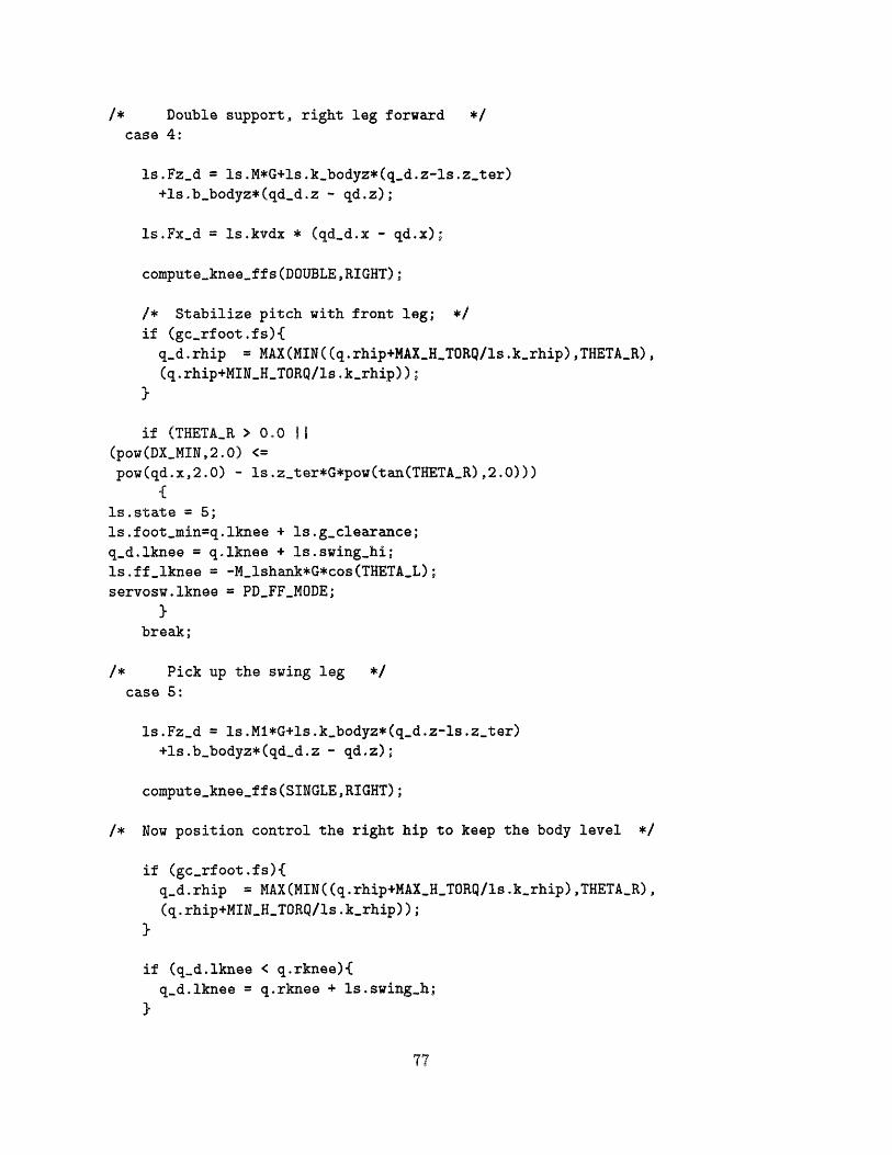
/* Double support, right leg forward */

case 4:

ls.Fzd = ls.M*G+ls.kbodyz*(qd.z-ls.zter)+ls.bbodyz*(qdd.z - qd.z);

ls.Fxd = ls.kvdx * (qd-d.x - qd.x);


/* Stabilize pitch with front leg; */

if (gcrfoot.fs){

qd.rhip = MAX(MIN((q.rhip+MAXHTORQ/ls.krhip),THETAR),(q.rhip+MINHTORQ/ls.krhip));

}

if (THETAR > O0 l

(pow(DXMIN,2.0) <=

pow(qd.x,2.0) - ls.zter*G*pow(tan(THETAR),2.0)))

{ls.state = 5;

ls.footmin=q.lknee + ls.gclearance;qd.lknee = q.lknee + ls.swinghi;

ls.fflknee = -Mlshank*G*cos(THETAL);servosw.lknee = PDFFMODE;

}break;

/* Pick up the swing leg */

case 5:

ls.Fzd = ls.M1*G+ls.kbodyz*(qd.z-ls.zter)+ls.bbodyz*(qdd.z - qd.z);

computekneeffs(SINGLE,RIGHT);

/* Now position control the right hip to keep the body level */

if (gcrfoot.fs){


}

if (qd.lknee < q.rknee){

qd.lknee = q.rknee + ls.swingh;

}

77

if (q.lknee > q.rknee && q.lknee > ls.footmin && !gclfoot.fs)

{ls.state = 6;

qd.lhip = MAX(MIN((q.lhip+MAXHTORQ/ls.klhip),(-THETAR - q.pitch + ls.swinglead)),

(q.lhip+MINHTORQ/ls.klhip));servosw.lhip = PDMODE;

servosw.lknee = PDMODE;

}break;

/* Move through single support on right leg */case 6:

ls.Fzd = ls.Mi*G+ls.kbodyz*(qd.z-1s. zter)+ls.bbodyz*(qdd.z - qd.z);

computekneeffs(SINGLE,RIGHT);

/* Mirror global angle of support leg with swing leg */

qd.lhip = MAX(MIN((q.lhip+MAXHTORQ/ls.klhip),(-THETAR - q.pitch + ls.swinglead)),

(q.lhip+MINHTORQ/ls.klhip));

if (q.lhip < 0 II qd.lknee < q.rknee){

qd.lknee = q.rknee + ls.swingh;

}


if (gcrfoot.fs){


if (THETAL < lstheta-min & q rhip > q.lhip){

ls.state = 7;

servosw.lknee = FFBMODE;

}

if (gclfoot.fs)

{if (q.rhip > q.lhip)

{

78

lsstate = 8;

servosw.lknee = FF_MODE;


adaptcontrol();

}else

{ls.state = 4;

ls.footmin=q.lknee + ls.gclearance;



}break;

/* Put the left leg back on the ground */

case 7:

ls.Fzd = ls.Ml*G+ls.kbodyz*(q-d.z-ls.zter)

+ls.bbodyz*(qdd.z - qd.z);

computekneeffs(SINGLEDOWN,RIGHT);

if (gcrfoot.fs){

qd.rhip = MAX(MIN((q.rhip+MAXHTORQ/ls.krhip),THETA_R),

(q.rhip+MINHTORQ/ls.krhip));

}

if (gclfoot.fs){

ls.state=8;

servosw.lknee = FFMODE;servosw.rhip = FFMODE;

adaptcontrol();

}break;

/* Double support, left leg forward */

case 8:


ls.Fxd = ls.kvdx * (qdd.x - qd.x);

computekneeffs(DOUBLE,LEFT);

79

if (gclfoot.fs){

qd.lhip = MAX(MIN((q.lhip+MAXHTORQ/ls.klhip),THETAL),(q.lhip+MINHTORQ/ls. khip));

}

if (THETAL > 0.0 II(pow(DXMIN,2.0) <=

pow(qd.x,2.0) - ls.zter*G*pow(tan(THETAL),2.0)))

{is.state = 9;

is.footmin=q.rknee + ls.gclearance;qd.rknee = q.rknee + ls.swinghi;Is.ffrknee = -Mrshank*G*cos(THETAR);servosw.rknee = PDFFMODE;

}break;

Pick up the swing leg (right leg) */

case 9:

Is.Fzd = s. M*G+ls.kbodyz*(qd.z-ls.zter)

+Is.bbodyz*(qdd.z - qd.z);

computekneeffs(SINGLE,LEFT);

/* Now position control the left hip to keep the body level */

if (gclfoot.fs){

qd.lhip = MAX(MIN((q.lhip+MAXHTORQ/ls.klhip),THETA_L),

(q.lhip+MINHTORQ/ls.klhip));

}

if (qd.rknee < q.lknee){

qd.rknee = q.lknee + ls.swingh;

if (q.rknee > q.lknee && q.rknee > ls.footmin && !gcrfoot.fs)

{is.state = 10;

qd.rhip = MAX(MIN((q.rhip+MAXHTORQ/ls.krhip),(-THETAL-q.pitch + ls.swinglead)),

(q.lhip+MINHTORQ/ls.klhip));servosw.rhip = PDMODE;

servosw.rknee = PDMODE;

80

break;

Move through single support on left leg */

case 10:

ls.Fzd = s.Ml*G+ls.kbodyz*(qd.z-ls.zter)+Ils.bbodyz*(qdd.z - qd.z);

computekneeffs(SINGLE,LEFT);


qd.rhip = MAX(MIN((q.rhip+MAXHTORQ/ls.krhip),(-THETAL-q.pitch + ls.swinglead)),

(q.rhip+MINHTORQ/ls.krhip));

if (q.rhip < 0 II qd.rknee q.lknee){

qd.rknee = q.lknee + s.swingh;}


if (gclfoot.fs){

qd.lhip = MAX(MIN((q.lhip+MAXHTORQ/ls.klhip),THETAL),(q.lhip+MINHTORQ/ls.klhip));

}

if (q.lhip>q.rhip && THETAR < ls.thetamin)

{ls.state = 11;

servosw.rknee = FFBMODE;

}

if (gcrfoot.fs)

{if (q.lhip > q.rhip)

{ls.state = 4;



adaptcontrol();

}else

{ls.state = 8;

qd.rknee = q.rknee + ls.swinghi;

81

servosw.rhip = FFMODE;servosw.rknee = FFMODE;

}break;

/* Put the right leg back on the ground */

case 11:

Is.Fzd = Is.Mi*G+ls.kbodyz*(qd.z-ls.zter)+Ils.bbodyz*(qdd.z - qd.z);

computekneeffs(SINGLEDOWN,LEFT);

if (gclfoot.fs){

qd.lhip = MAX(MIN((q.lhip+MAXHTORQ/ls.klhip),THETAL),(q.lhip+MINHTORQ/ls. klhip));

}

if (gcrfoot.fs)

{ls.state=4;



adaptcontrol();

}break;

default:

ls.klhip = HIPK;ls.klknee = KNEEK;is.krhip = HIPK;ls.krknee = KNEEK;

qd.lknee = -0.1;

qd.rknee = -0.1;qd.lhip = -0.13;

qd.rhip = 0.13;

break;

/* **************************************************************onrol

adaptcontrol()

82

Called to calculate terrain data and virtual leg data

void adaptcontrol()

{

double lfootx,lfootz,rfootx,rfootz,factor;

ls.terz = terrainzatxy(q.x,0.O);

ls zter = q.z - ls.terz;

Is.qrvleg = THIGHZ+SHANKZ-q.rknee;

is.qlvleg = THIGHZ+SHANKZ-q.lknee;

ls.qrfoota = THETAR;

ls.qlfoota = THETAL;

lfootx = -(ls.qlvleg)*sin(THETAL);rfootx = -(ls.qrvleg)*sin(THETAR);

lfootz = (Is.qlvleg)*cos(THETAL);

rfootz = (is.qrvleg)*cos(THETAL);

if (gcrfoot.fs){

ls.rmu=ABS((gcrfoot.fz*sin(ls.groundangle)+gcrfoot.fx*cos(ls.groundangle))/(-gcrfoot.fz*cos(ls.groundangle)+gcrfoot.fx*sin(ls.groundangle)));

}else ls.r_mu = 0.0;

if (gclfoot.fs){

is. _mu=ABS((gclfoot.fz*sin(ls.groundangle)

+gclfoot.fx*cos (is.groundangle))/

(-gclfoot.fz*cos (is.groundangle)

+gclfoot.fx*sin(ls.groundangle)));

}

else ls.lmu = 0.0;

if (gcrfoot.fs && gclfoot.fs && ls.state>1)

if (s.qrfoota < ls.qlfoota){

Is.groundangle = atan2(rfootz-lfootz,lfootx-rfootx);}

elsef

ls.groundangle = atan2(lfootz-rfootz,rfootx-lfootx);}

}

if (is.ground_angle > 0.0)

83

factor = MAX(O,(MAXTERRAINANGLE

- ls.groundangle)/MAXTERRAINANGLE);

}

setdampingfromkzeta()Called to take ls.k_((l/r)(knee/hip)/bodyz) and

ls.zeta_(hip/knee/bodyz) and set b(knee/hip/bodyz)

to required values.

Using CG's of thigh and shank at half extension for MoI,

body plus thigh mass for bodyz controller, and body plus thigh

mass for bodydx controller************************************************************** */

void setdampingfromkzeta()

{double i=(Mlthigh*pow(THIGHZ/2.0,2.0)

+ Mlshank*pow(THIGHZ,2.0))/3.0;

Is.blhip = 2.0*ls.zetahip*sqrt(ls.klhip*i);

is .blknee = 2.0*ls.zetaknee*sqrt (is .klknee*Mlshank);is.brhip = 2.0*ls.zetahip*sqrt(ls.krhip*i);

Is.brknee = 2.0*ls.zetaknee*sqrt(ls.krknee*Mrshank);

is.bbodyz = 2.0*ls.zetaknee*sqrt (s.kbodyz*ls.M);

/* ***************$***************************************computekneeffs(support, supside)Called to set ls.ffrknee and ls.fflknee from ls.Fxd

and ls.Fzd***************************************$********************** */

void computekneeffs(support, supside)

int support;

int supside;

int i;

double ff[2;

double theta[2],hipdif [2J;

theta[LEFT] = THETAL;

84

theta[RIGHT] = THETAR;

hipdif[LEFT] = q.lhip-q.rhip;

hipdif[RIGHT] = q.rhip-q.lhip;

if (support == DOUBLE)

{

/* Calculate desired feed forward forces */

ff[!supside = (s.Fzd * sin(theta[supside])

- ls.Fxd * cos(theta[supside]))/sin(hipdif[!supsideD);

ff[supside] = (ls.Fzd * sin(theta[Csupside])

- ls.Fxd * cos(theta[!supside]))/sin(hipdif [supsidel);

/* Check to make sure the feet aren't

for (i=O;i<2;i++)

being pulled up */

if (ff[i] > FKNEE.MAX)

{ff[i] = FKNEEMAX;

ff [! i = (FKNEEMAX*cos(theta[! i])

-Is.Fzd)/cos(theta[i]);

}

}

else

{ffEsupside] = MIN((-ls.Fz_d/cos(theta~supside])),FKNEE_MAX);

if (support==SINGLEDOWN) {

ff[!supside] = FKNEEDOWN;

}else{

ff[!supside] = Mlshank*G*cos(theta[!supside]);

}}

ls.fflknee = MIN(MAX(ff C[LEFT],FKNEEMIN) ,-F_KNEE_MIN);

ls.ffrknee = MIN(MAX(ff[RIGHT],FKNEEMIN),-FKNEEMIN);}

/* **************************************************************

85

onetimeinit()

Called to do one-time setup for control algorithm

void onetimeinit()

{

ls.t = 0.0;

ls.M = Mbody+Mlthigh+Mrthigh;

ls.M1= Is.M + Mlshank;

ls.kvdx = DX_KV;

gcrfoot.model = 101.0;

gclfoot.model = 101.0;

ls.thetamin = THETAMIN;ls.swinglead = SWINGLEAD;

ls.swinghi = SWINGHI;ls.swingh = SWINGH;ls.gclearance = GCLEARANCE;

ls.klhip = HIP_K;

ls.klknee = KNEEK;Is.krhip = HIP_K;

ls.krknee = KNEEK;ls.kbodyz = BODYZ_K;

ls.zetaknee = KNEEZETA;ls.zetahip = HIPZETA;ls.zetabodyz= BODYZ_ZETA;

ls.zetabodydx = BODYDXZETA;


ls.bffb = BKNEEDOWN;

ls.groundangle = 0.0;

gcrfoot.kz = 1000.0;gc-lfoot okz = 1000.0;gcrfoot.kx = gcrfoot.kz;gclfoot.kx = gclfoot.kz;gcrfoot.ky = 0.0;gclfoot.ky = 0.0;

gcrfoot.bz = 500.0;

gclfoot.bz = 500.0;

86

gcrfoot.bx = 500.0;

gclfoot.bx = 00.0;

gcrfoot.by = 0.0;

gclfoot.by = 0.0;

ls.k_ff = FFK;lsob_ff = FF_B;

qd.z = ZNOM;ls.dxmin = DXMIN;qdd.x = DXNOM;qd_d.z = 0.0;

/* *************************************************************initcontrol()

Called to initialize or reset the control algorithm.************************************************************** */

void initcontrol()

{

q.z = ZNOM;

q.x = 0.0;

qd.x = 0.0;

qd.z = 0.0;

ls.Fzd = ls.M*G;

ls.Fxd = 0.0;

qd.lhip = INITHIP;qd.lknee = (ZNOM)/cos(THETAL) - THIGHZ;qd.rhip = -INITHIP;qd.rknee = (ZNOM)/cos(THETAR) - THIGHZ;

q.lhip = INITHIP;

q.lknee = (ZNOM)/cos(THETAL) - THIGHZ;q.rhip = -INITHIP;

q.rknee = (ZNOM)/cos(THETAR) - THIGHZ;

ls.ff_lhip = 0.0;

ls.ff_rhip = 0.0;


servosw.lhip = PD_FFMODE;

servosw.lknee = PD_FFMODE;

servosw.rhip = PDFF-MODE;

87

servosw.rknee = PD_FF_MODE;

}

/* *************************************************************usergcontact()

called with a contact point. This is to allow user-defined

ground contact - set the contact type to something over 100,

like with servos.

The parameters are the ground contact structure, the

position of the ground contact in global coordinates, and

the velocity of the ground contact in global coordinates.

************************************************************** */

void

user_gcontact(contact, x, y, z, dx, dy, dz)

basicgcontact *contact;

double x, y, z, dx, dy, dz;

{-

double f[3], p[3], g[C3, v3, theta, dtheta;

g[0] = z;g[ll = x;

g[2] = y;

/* sdpos(link, p, g);

sdvel(link, p, v); */

/* Now you have g = position (z,x,y) of the contact point

in the ground frame */

contact->atx = gll;

contact->aty = g[2];

contact->atz = g[O];

contact->atth = 0.0;

switch ((int)(contact->model))

{case iO1:

linearspringdamperterrain(contact, x, y, z, dx, dy, dz);

/* or DOGHNUT */

break;

88

__ ___. -- ^- ... - ---- _- - -r--· ................... '-- _s :'- 5,, ,- -,w 2bs-i C o --- -

default:

contact->fx = 0.0;

contact->fy = 0.0;

contact->fz = 0.0;

break;

}

C.2 KWALKB Control CodeFollowing are the functions I wrote to implement the KWALKB control systemwithin the structure of the existing simulation package. The usergcontact is partof Peter Dilworth's terrain module.

/* **************************************************************controli()

Called every control cycle. Should contain or call the actual

creature control code.************************************************************** */

void

controli()

adaptcontrol();

switch ((int)ls.state) {

Initialize robotcase 0:

onetimeinit();

ls.state=i;

break;

case 1:

initcontrol();

ls.state=2;

89

break;

case 2:

/* Wait here for transients to settle out */

solveleg(LEFT);

solveleg(RIGHT);

if(ls.t>0.3){

ls.state = 3;

ls.fflhip = 0.0;

ls.fflknee = 0.0;

ls.ffrknee = 0.0;





}

break;

case 3:

/* Command knee torques to stay upright, keep zero torque

at left hip, and position control the right hip to keep

pitch at zero */


ls.Fx-d = 00;

if (gcrfoot.fs){

qd.rhip = THETAR;

}

torquesfromforces(DOUBLE,RIGHT);

if(ls.t>0.4)

{Is.state = 4;

/* Soften position control for picking up and putting

down legs */

ls.klknee = KNEEAIRK;ls.krknee = KNEEAIRK;

90

setdampingfromkzeta();servosw.lhip = FFMODE;




}break;

/* Double support, right leg forward */

case 4:

is.Fzd = s.M*G+ls.kbodyz*(qd.z-ls.zter)+Ils.bbodyz*(qdd.z - qd.z);


/* Stabilize pitch with front leg; */

if (gcrfoot.fs){

qd.rhip = THETAR;

}

torquesfromforces(DOUBLE,RIGHT);

if ( ls.qrfoota > 0.0 II

(pow(ls.dxmin,2.0) <=

pow(qd.x,2.0) - ls.zter*G*pow(tan(ls.qrfoota),2.0)))

{ls.state = 5;is.footmin=ls.qlvleg - is.gclearance;ls.qdlvleg = ls.qlvleg - ls.swinghi;solveleg(LEFT);

servosw.lknee = PD_MODE;

servosw.lhip = PDMODE;

}break;

Pick up the swing leg */

case 5:

is.Fzd = s.Mi*G+ls.kbodyz*(qd.z-ls.zter)+ls.bbodyz*(qdd.z - qd.z);


if (gcrfoot.fs){

91

qd.rhip = THETAR;

if (ls.qdlvleg > ls.qrvleg){

ls.qdlvleg = ls.qrvleg - ls.swingh;

}

solveleg(LEFT);

torquesfromforces(SINGLE,RIGHT);

if (((ls.qlvleg < ls.qrvleg && ls.qlvleg < ls.footmin) il

ls.qlfoota < ls.qrfoota) && !gclfoot.fs){ls.state = 6;

ls.qdlfoota = -ls.qrfoota + ls.swinglead;solveleg(LEFT);

}

break;

/* Move through single support on right leg */

case 6:

ls.Fzd = ls.Ml*G+ls.kbodyz*(qd.z-ls.zter)+ls.bbodyz*(qdd.z - qd.z);


ls.qdlfoota = MAX(-ls.qrfoota+ls.swinglead, 1 .2*ls.thetamin);

/* Make sure swing foot stays above support foot */

if (ls.qd_lfoota < 0 II ls.qdlfoota > ls.qrfoota){

ls.qdlvleg = ls.qrvleg - ls.swingh;


if (gc-rfootfs){qd.rhip = THETAR;

solveleg(LEFT);


if (ls.q_lfoota < ls.thetamin && ls.qrfoota > ls.qlfoota){

92

lsostate = 7;

servosw.lknee =

servosw.lhip =

}

if (gclfoot.fs){

if (ls.qrfoota

ls.state = 8;

servosw.lknee = FFMOE

servosw.rhip = FFMOE

}else {

ls.state = 5;

Is.footmin=ls.qlvleg

}

break;

FF_BMODE;FF_B_MODE;

> ls.qlfoota){

DE;

E;

- ls.g_clearance;

/* Put the left leg back on the ground */

case 7:

ls.Fzd = ls.M1*G+ls.kbodyz*(qd.z-ls.zter)+ls.bbodyz*(qdd.z - qd.z);

if (gcrfoot.fs){

qd.rhip = THETAR;


torquesfromforces(SINGLEDOWN,RIGHT);

if (gclfoot.fs){

is.state=8;

servosw.lknee = FF_MODE;


servosw.lhip = PDMODE;

}break;

Double support, left leg forward */case 8:


93


torquesfromforces(DOUBLELEFT);

if (gclfoot.fs){

qd.lhip = THETAL;

}

if (ls.qlfoota > 0.0 I

(pow(ls.dxmin,2.0) <=

pow(qd.x,2.0) - ls.zter*G*pow(tan(ls.qlfoota),2.0)))

{ls.state = 9;

ls.footmin=ls.qrvleg - ls.gclearance;ls.qdrvleg = ls.qrvleg - ls.swinghi;solveleg(RIGHT);

servosw.rknee = PDMODE;


}break;

/* Pick up the swing leg (right leg) */

case 9:



if (gclfoot.fs){

qd.lhip = THETAL;

torquesfromforces(SINGLE,LEFT);

if (ls.q_d_rvleg < ls.qlvleg){

ls.qdrvleg = ls.qlvleg - ls.swingh;

}

solveleg(RIGHT);

if (((ls.qrvleg < ls oqlvleg && ls q-rvleg < ls.foot.min) |

(ls oqrfoota<lsqlfoota)) &&. !gcrfoot fs)

ls.state = 10;

ls.qdrfoota = -ls.qlfoota + s.swinglead;

94

solveleg(RIGHT);

}break;

/* Move through single support on left leg */

case 10:



ls.qdrfoota = MAX(-ls.qlfoota+ls.swinglead,1.2*ls.thetamin);

if (ls.qrfoota < 0 II ls.qdrfoota < ls.qlfoota){

ls.qdrvleg = ls.qlvleg - ls.swingh;

}


if (gclfoot.fs){

qd.lhip = THETAL;

}

solveleg(RIGHT);


if (ls.qlfoota > ls.qrfoota && ls.qrfoota < ls.thetamin)

{ls.state = 11;

servosw.rknee = FF_B_MODE;

servosw.rhip = FF_BMODE;

}

if (gcrfoot.fs)

if (ls.qlfoota > ls.qrlfoota)

{ls.state = 4;



}else

{ls.state = 9;

95

ls.qdrvleg = ls.qrvleg - Is.swinghi;}

break;

/* Put the right leg back on the ground */

case 11:

Is.Fzd = s.M1*G+ls.kbodyz*(qd.z-ls.zter)+ls.bbodyz*(qdd.z - qd.z);

if (gclfoot.fs){

qd.lhip = THETAL;

}


torquesfromforces(SINGLEDOWN,LEFT);

if (gcrfoot.fs)

{Is.state=4;




}break;

default:

Is.klhip = HIPK;Is.klknee = KNEEK;

is.krhip = HIPK;is.krknee = KNEEK;

qd.lknee = -0.1;

qd.rknee = -0.1;

qd.lhip = -0.13;

qd.rhip = 0.13;

break;

setdampingfromkzeta()Called to take ls.k_((l/r)(knee/hip)/bodyz) and

ls.zeta_(hip/knee/bodyz) and set b_(knee/hip/bodyz) to

96

required values.Using CG's of thigh and shank at half extension for MoI,

body plus thigh mass for bodyz controller, and body plus thigh

mass for bodydx controller

void setdampingfromkzeta(){

double i=(Mlthigh*pow(THIGHZ/2.0,2.0)

+ Mlshank*pow(THIGHZ+SHANK.Z/2.0,2.0))/3.0;double il = Mlshank*pow(SHANK._Z/2.0,2.0)/3.0;

is.blhip = 2.0*ls.zetahip*sqrt(ls.k.lhip*i);

Is.blknee = 2.0*ls.zetaknee*sqrt(ls.klknee*il);

is.brhip = 2.0*ls.zetahip*sqrt(ls.krhip*i);

Is.brknee = 2.0*ls.zetaknee*sqrt(ls.krknee*il);

Is.bbodyz = 2.0*ls.zetaknee*sqrt(ls.kbodyz*ls.M);

adaptcontrol()

Called to calculate data from terrain and virtual model

void adaptcontrol()

double lfootx,lfootz,rfootx,rfootz,factor;

ls.terz = terrainzatxy(q.x,0.0);

Is.zter = q.z - s.terz;

/* Calculate the virtual leg length and angle */

ls.qlvleg = MIN(THIGHZ+SHANKZ,pow(THIGHZ*THIGHZ+SHANKZ*SHANKZ

+2.0*THIGHZ*SHANKZ*cos(q.lknee),0.5));

is.qrvleg = MIN(THIGHZ+SHANKZ,pow(THIGHZ*THIGHZ+SHANKZ*SHANKZ

+2.0*THIGHZ*SHANKZ*cos(q.rknee),0.5));

ls.qlfoota = THETAL -Is.invert*acos((ls.qlvleg*ls.qlvleg+THIGHZ*THIGHZ-SHANKZ*SHANKZ)/(2.0*THIGHZ*ls. q.lvleg));

Is.qrfoota = THETAR -is.invert*acos((ls.qrvleg*ls. qrvleg+THIGHZ*THIGHZ

97

-SHANKZ*SHANKZ)/(2.0*THIGHZ*ls.qrvleg));

ls.thetar = THETAR;ls.thetal = THETAL;

lfootx = -(ls.qlvleg)*sin(THETAL);

rfootx = -(ls..qrvleg)*sin(THETAR);

lfootz = (ls.qlvleg)*cos(THETAL);

rfootz = (is.qrvleg)*cos(THETAL);

if (gcrfoot.fs){

ls.rmu=ABS((gcrfoot.fz*sin(ls.groundangle)+gcrfoot.fx*cos(ls.groundangle))/(-gcrfoot.fz*cos(ls.groundangle)+gcrfoot.fx*sin(ls.groundangle)));

}else ls.r_mu = 0;

if (gclfoot.fs){

ls.1_mu=ABS((gclfoot.fz*sin(ls.groundangle)

+gclfoot.fx*cos(ls.groundangle))/(-gclfoot.fz*cos(ls.groundangle)+gclfoot.fx*sin(ls.groundangle)));

}else ls.lmu = 0;

if (gcrfoot.fs && gclfoot.fs && s.state>l)

if (s.qrfoota < ls.qlfoota){

ls.groundangle = atan2(rfootz-lfootz,lfootx-rfootx);}

else{

is.groundangle = atan2(lfootz-rfootz,rfootx-lfootx);}

}

torquesfromforces() takes the support type, support leg,

and calculates the required knee torques************************************************************** */

void torquesfromforces(support,supside)char support;

char supside;

{

int i;

98

double theta[2] [3];double alpha[2],footdif [2] ,ff[2];

double qvleg[2];

theta[RIGHT] [KNEE] = q.rknee;

theta[LEFT] [KNEE] = q.lknee;

theta[RIGHT] [HIP] = THETAR;

theta[LEFT] [HIP] = THETAL;theta[RIGHT][FOOT] = ls.qrfoota;theta[LEFT][FOOT] = ls.qlfoota;

qvleg[RIGHT]=ls.qrvleg;qvleg[LEFT] =ls.qlvleg;

footdif[LEFT] = ls.qlfoota-ls.qrfoota;footdif[RIGHT] = ls.qrfoota-ls.qlfoota;

alpha[LEFT] = 2*asin(Is.qlvleg/(THIGHZ+SHANKZ));

alpha[RIGHT] = 2*asin(ls.qrvleg/(THIGHZ+SHANKZ));

/* Calculate feed forward forces for virtual leg */

if (support==DOUBLE)

{/* Calculate desired feed forward forces */

ff[!supside] = (is.Fzd * sin(theta[supside] [FOOT])

- ls.Fxd * cos(theta[supside][FOOT]))/sin(footdif[! supside]);

ff[supside] = (ls.Fzd * sin(theta[!supside] [FOOT])

- ls.Fxd * cos(theta[!supside] [FOOT]))/sin(footdif[supside]);

/* Check to make sure the feet aren't being pulled up */

for (i=O;i<2;i++)

if (ff[i] > FKNEEMAX)

{ff[i] = FKNEEMAX;

ff [! i] = (FKNEEMAX*cos(theta[! i] [FOOT])-ls.Fzd)

/cos(theta[i] [FOOT]);

}}

else

99

{ff [supside] = MIN((-ls.Fzd/cos(theta[supside] [FOOT]))

,FKNEEMAX);if (support==SINGLEDOWN) (

ff[!supside] = FKNEEDOWN;

}else{

ff [!supside] = Mlshank*G*cos(theta[! supside] [FOOT]);

/* Now convert to knee torques, keeping in the actuator limits */

ls.fflknee = MAX(ls.minktorq,MIN(ls.maxktorq,

-is.invert*ff [LEFT] * (THIGHZ+SHANKZ)

*cos(alpha[LEFT]/2.0)/2.0));

Is.ffrknee = MAX(ls.minktorq,MIN(ls.maxktorq,

-Is.invert*ff[RIGHT] * (THIGH_Z+SHANK_Z)

*cos(alpha[RIGHT]/2.0)/2.0));

if (supside==RIGHT)

ls.fflhip = 0.0;

}else{

ls.ff_rhip = 0.0;

/* **************************************************************solveleg(side)

sets q.knee and q.hip for the desired leg to put the foot in place

************************************************************* */void solveleg(side)

char side;

{double calpha, salpha; /* cos of angle between knee and thigh */

double cbeta; /* cos of angle between virtual leg and thigh */

double knee,hip,vleg2,foota,footd;

if (side==LEFT)

{foota = ls.qdlfoota;

footd = ls.qdlvleg;

100

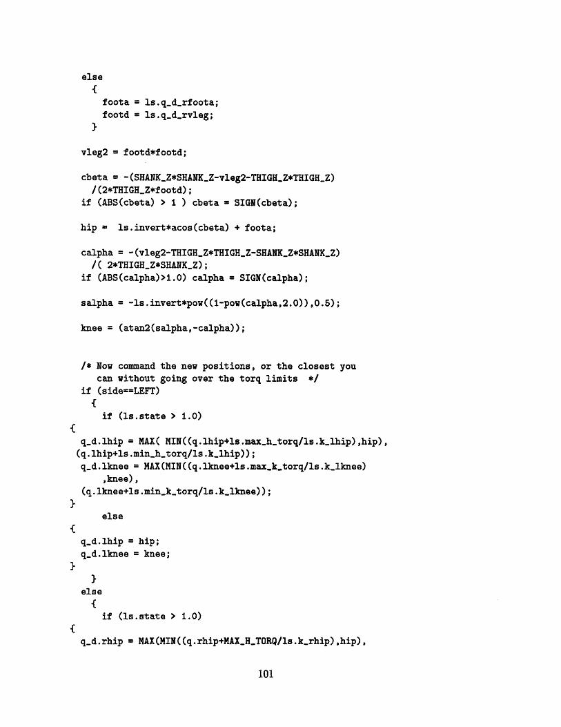
else

{foota = ls.qdrfoota;

footd = ls.qdrvleg;

}

vleg2 = footd*footd;

cbeta = -(SHANKZ*SHANKZ-vleg2-THIGHZ*THIGHZ)

/(2*THIGHZ*footd);

if (ABS(cbeta) > ) cbeta = SIGN(cbeta);

hip = ls.invert*acos(cbeta) + foota;

calpha = -(vleg2-THIGHZ*THIGHZ-SHANKZ*SHANKZ)

/( 2*THIGHZ*SHANKZ);if (ABS(calpha)>i.O) calpha = SIGN(calpha);

salpha = -s.invert*pow((1-pow(calpha,2.0)),0.5);

knee = (atan2(salpha,-calpha));

/* Now command the new positions, or the closest you

can without going over the torq limits */

if (side==LEFT)

{if (ls.state > 1.0)

qd.lhip = MAX( MIN((q.lhip+ls.maxhtorq/ls.klhip),hip),

(q.lhip+ls.minhtorq/ls.klhip));qd.lknee = MAX(MIN((q.lknee+ls.maxktorq/ls.klknee)

,knee),

(q.lknee+ls.minktorq/ls.klknee));

else

qd.lhip = hip;

qd.lknee = knee;

}

else

if (Is.state > 1.0)

qd.rhip = MAX(MIN((q.rhip+MAXHTORQ/ls.krhip),hip),

101

(q.rhip+MINHTORQ/ls. krhip));qd.rknee = MAX(MIN((q.rknee+MAXKTORQ/ls.krknee),knee),(q.rknee+MINKTORQ/ls.krknee));

else

qd.rhip = hip;

q_d.rknee = knee;

/* onetime**************************************************************onetimeinit ()Called to initialize parameters for first run.

void onetimeinit()

{ls.M = Mbody;

ls.Ml= ls.M + Mlshank + Mlthigh;

ls.kvdx = DXKV;

gcrfoot.model = 101.0;

gclfoot.model = 101.0;

ls.thetamin = THETAMIN;ls.swinglead = SWINGLEAD;

ls.swinghi = SWINGHI;ls.swingh = SWINGH;ls.gclearance = GCLEARANCE;

ls.invert = INVERT; /* Knee inversion -l=forward, 1 backward */

ls.klhip = HIPK;ls.klknee = KNEEK;ls.krhip = HIPK;ls.krknee = KNEEK;ls.kbodyz = BODYZK;

ls.maxktorq = MAXKTORQ;ls.minktorq = MINKTORQ;ls.maxhtorq = MAXHTORQ;ls.minhtorq = MINHTORQ;

102

ls.zetaknee = KNEEZETA;is.zeta-hip = HIPZETA;ls.zetabodyz= BODYZZETA;

ls.zetabodydx = BODYDXZETA;


ls.bffb = BKNEEDOWN;

gcrfoot.kz = 1000.0;

gclfoot.kz = 1000.0;

gcrfoot.kx = gcrfoot.kz;gclfoot.kx = gclfoot.kz;gcrfoot.ky = 0.0;

gclfoot.ky = 0.0;

gcrfoot.bz = 500.0;

gclfoot.bz = 500.0;

gcrfoot.bx = 500.0;

gclfoot.bx = 500.0;

gcrfoot.by = 0.0;

gclfoot.by = 0.0;

ls.kff = FFK;ls.bff = FFB;

initcontrol()Called to initialize the control algorithm.************************************************************** */

void initcontrol()

{

ls.t = 0.0;

ls.Fzd = ls.M*G;

ls.Fx_d = 0.0;

Is. qdrfoota=-INIT_FOOTA;ls. qdrvleg=INITFOOTD;Is.qdlfoota=INITFOOTA;ls.qdlvleg=INITFOOTD;

solveleg(LEFT);

solveleg(RIGHT);

103

qd.z = INITFOOTD*cos(INITFOOTA);

q.lhip = qd.lhip;

q.lknee = qd.lknee;

q.rhip = qd.rhip;

q.rknee = qd.rknee;

q.z = qd.z;

ls.dxmin = DXMIN;qdd.x = DXNOM;qdd.z = 0.0;

ls.fflhip = 0.0;

ls.ff_lknee = 0.0;

ls.ffrhip = 0.0;

ls.ffrknee = 0.0;

servosw.lhip = PDFFMODE;

servosw.lknee = PDFFMODE;

servosw.rhip = PDFFMODE;

servosw.rknee = PDFFMODE;

/* **************************************************************usergcontact()

called with a contact point. This is to allow user-defined

ground contact - set the contact type to something over 100,

like with servos.

The parameters are the ground contact structure, the position

of the ground contact in global coordinates, and the velocity

of the ground contact in global coordinates.

************************************************************** */

void usergcontact(contact, x, y, z, dx, dy, dz)

basicgcontact *contact;


{

double f[3], p[3], g[3], v[3, theta, dtheta;

gCo] = z;gEl]= x;g[2] = y;

104

/* Now you have g = position (z,x,y) of the contact point

in the ground frame */

contact->atx = gl;contact->aty = g[2;contact->atz = g[O];

contact->atth = 0.0;

switch ((int)(contact->model))

{case 101:

linearspringdamperterrain(contact, x, y, z, dx, dy, dz);

/* or DOGHNUT */break;

default:

contact->fx = 0.0;

contact->fy = 0.0;

contact->fz = 0.0;

break;

}

105

Appendix D

Simulation Code

The simulation system in the M.I.T. Leg Lab automatically produces the file main.c.As this is unpublished proprietary information, I will list only Peter Dilworth'smodifications made to add his rough terrain module.

D.1 Modifications to Main.c

/* BEGIN USER CODE 1 */

/* To read in a terrain file */

#define TERRAIN (LASTSIMCOMMAND + 1)

terraindata td; /* PCD */

/* END USER CODE 1 */


"TER", /* 14 */



goalfileinitialize();


/* BEGIN USER

} else {

block =

Display

CODE 4 */

1;

(vars); /* library */

107

Y

}/* END USER CODE 4 */




case TERRAIN:

if (nwords == 1i)

ErrDisplay("load what terrain file?");

else

if (loadterrain(words [1]))

{ErrDisplay("Terrain file loaded");

}

break;



/* Code from here to end is compliments of Peter Dilworth,

staff of the MIT Leg Lab since June 1994. */

this returns:

O -- if the foot did not hit the ground,

i -- if the foot landed on terrain,-1 -- if the foot landed outside terrain

there are two modes:

td.mapmode = REGIONMODE --> foot may land outside terrain

(z = 0 in all cases)

td.mapmode = DOGHNUTMODE -- > foot always lands inside terrain,

edges wrap around

double checkforterrainhit( x, y, z )

double x;

108

double y;

double z;

double offsetx, offsety;

double xslope, yslope;

double deltay, deltax, deltaz;

double Ox, Oy, Xx, Xy, Yx, Yy;

int result = 0.0;

int which;

/* if region mode, see if leg is over terrain patch at all */

if((td.mapmode == REGIONMODE) &&

((x < (td.xoffset*td.xres)) I(x >= ((td.xoffset+td.xdim)*td.xres)) II(y < (td.yoffset*td.yres)) II(y >= ((td.yoffset+(td.ydim-l.0))*td.yres))))

/* foot is over flat default ground in region mode,

flat ground z = zero everywhere */

if(z < 0.0)

{result = -1.0;

}

else

{/* either REGION or DOGHNUT mode (it doesn't matter which)

but foot is over terrain map *//* if in REGION mode, convert absolute foot coords into

relative offset coords for use with terrain array check */

if(td.mapmode == REGIONMODE)

{/* convert point from linear world coords to linear

terrain coords */

offsetx = (x - (td.xoffset*td.xres));

offsety = (y - (td.yoffset*td.yres));

which = getterraincornerpoints

(offsetx, offsety, &Ox, Oy, &Xx, &Xy, &Yx, &Yy);

}else

/* td.mapmode == DOGHNUTMODE */

/* wrap hit point around terrain using modulus function

and resolve into linear terrain coords */

offsetx = fmod(x, (td.xdim*td.xres));

109

offsety = fmod(y, ((td.ydim-l.O)*td.yres));


(offsetx, offsety, Ox, Oy, &Xx, &Xy, &Yx, &Yy);

}

td.Oz = td.terrainarray[((int)Oy*(int)td.xdim)+(int)Ox];

td.Xz = td.terrainarray[((int)Xy*(int)td.xdim)+(int)Xx];

td.Yz = td.terrainarray[((int)Yy*(int)td.xdim)+(int)Yx];

/* get z values for corners of (possible) hit triangle */

/* see if foot is actually touching ground */

xslope = ((td.Xz-td.Oz)*td.zres)/td.xres;

yslope = ((td.Yz-td.Oz)*td.zres)/td.yres;

if(which == LOWER)

{/* origin point of triangle is corner of grid square

closest to world origin */

deltax = fmod(offsetx, td.xres);

deltay = fmod(offsety, td.yres);

else /* UPPER triangle */

/* origin point of triangle is corner of grid square on

opposite side from world origin, hence flip */

deltax = td.xres - fmod(offsetx, td.xres);

deltay = td.yres - fmod(offsety, td.yres);

}

deltaz = (xslope*deltax) + (yslope*deltay);

/* z of point right below foot on terrain */

td.Tz = (td.Oz*td.zres) + deltaz;

/* if it is, return 1.0 */

if(z < td.Tz)

{result = 1.0;

}

return(result);

}

like checkforterrainhit, but it just returns z height

110

of terrain below x,y

double terrainzatxy( x , y )double x;

double y;

{double offsetx, offsety;

double xslope, yslope;

double deltay, deltax, deltaz;

double Ox, Oy, Xx, Xy, Yx, Yy;

double tdXz, tdOz, tdYz;

double result = 0.0;

int which;

/* if region mode, see if leg is over terrain patch at all */if((td.mapmode == REGIONMODE) &&

((x < (td.xoffset*td.xres)) I(x >= ((td.xoffset+td.xdim)*td.xres)) II(y < (td.yoffset*td.yres)) II

(y >= ((td.yoffset+(td.ydim-l.0))*td.yres))))

result = 0.0;

else

{/* either REGION or DOGHNUT mode (it doesn't matter which),

but foot is over terrain map */

/* if in REGION mode, convert absolute foot coords into

relative offset coords for use with terrain array check */if(td.mapmode == REGIONMODE)

{/* convert point from linear world coords to

linear terrain coords */

offsetx = (x - (td.xoffset*tdoxres));

offsety = (y - (td.yoffset*tdyres));


(offsetx, offsety, &Ox, &Oy, &Xx, Xy, &Yx, &Yy);

}else

/* td.mapmode == DOGHNUTMODE */

/* wrap hit point around terrain using modulus function

and resolve into linear terrain coords */

offsetx = fmod(x, (td.xdim*td.xres));

111

offsety = fmod(y, ((td.ydim-l.O)*td.yres));


(offsetx, offsety, &Ox, &Oy, Xx, &Xy, &Yx, &Yy);

}

tdOz = td.terrainarray[((int)Oy*(int)td.xdim)+(int)Ox];

tdXz = td.terrainarray[((int)Xy*(int)td.xdim)+(int)Xx];

tdYz = td.terrainarray[((int)Yy*(int)td.xdim)+(int)Yx];

/* get z values for corners of (possible) hit triangle */

/* see if foot is actually touching ground */

xslope = ((tdXz-tdOz)*td.zres)/td.xres;

yslope = ((tdYz-tdOz)*td.zres)/td.yres;

if(which == LOWER)

{/* origin point of triangle is corner of grid square

closest to world origin */

deltax = fmod(offsetx, td.xres);

deltay = fmod(offsety, td.yres);

}else /* UPPER triangle */

{/* origin point of triangle is corner of grid square on

opposite side from world origin, hence flip */

deltax = td.xres - fmod(offsetx, td.xres);

deltay = td.yres - fmod(offsety, td.yres);

}

deltaz = (xslope*deltax) + (yslope*deltay);

/* z of point right below foot on terrain */

result = (tdOz*td.zres) + deltaz;

return(result);

}

determines the ordinates of the three corner points that

define the triangle of the terrain array that contain the

possible foot landing point Note: point defined by x, y

should be GUARANTEED to be in range

of terrain array, if it is not, something is terribly, terribly

wrong...

112

returns: UPPER or LOWER to specify which triangle pointis inside of

int getterraincornerpoints( x, y, Ox, Oy, Xx, Xy, Yx, Yy )double x;

double y;

double *Ox;

double *Oy;

double *Xx;

double *Xy;

double *Yx;

double *Yy;

double Sx, Sy;

int il, i2;

int result;

double lowerdist, upper_dist;

/* first find out which grid square you are in */

/* find corner of this grid closest to world origin */ii = (int)(x/td.xres);

i2 = (int)(y/td.yres);

Sx = (double)il;

Sy = (double)i2;

/* then find out which of the two possible origin corners isclosest to point, this defines UPPER vrs LOWER corner *

lowerdist = dist((Sx*td.xres), (Sy*td.yres), x, y);upperdist = dist(((Sx+1.O)*td.xres), ((Sy+1.O)*td.yres), x, y);

if(lowerdist < upperdist)result = LOWER;

else

result = UPPER;

/* fill in three corner points of triangle */

if(result == LOWER)

{*Ox = Sx;

*Oy = Sy;

*Xx = Sx+1.O;

*Xy = Sy;*Yx = Sx;

113

else

*Ox = Sx+1.O;

*Oy = Sy+1.O;

*Xx = Sx;

*Xy = Sy+1.O;

*Yx = Sx+l.O;

*Yy = Sy;

return(result);

}

just finds the distance between two points

double dist( x, yl, x2, y2 )

double xl;

double yl;

double x2;

double y2;

double result;

result = sqrt(((xl-x2)*(xl-x2))+((yl-y2)*(yl-y2)));

return(result);

first pass at custom terrain, implements normal linear

spring damper gc code, but uses terrain loaded into terrain

structure instead of flat ground.

there are two modes:

td.mapmode = REGIONMODE, where terrain maps ontoa patch whose origin is located at xoffset #yoffset

td.mapmode = DOGHNUTMODE, where terrain wraps around

at the edges like a toroid

void linearspringdamperterrain(gc, x, y, z, dx, dy, dz)

basicgcontact *gc;

114


double newfs;

/* get current state of foot switch */

newfs = checkforterrainhit(x, y, z);

if(newfs == 0.0)

{/* foot is off ground do nothing */

gc->fs = 0.0;

gc->fx = 0.0;

gc->fy = 0.0;

gc->fz = 0.0;

gc->tth = 0.0;

else

/* initial touchdown coordinate record */

if(gc->fs == 0.0)

{gc->tdx = x;

gc->tdy = y;

gc->tdz = z;

/* record that foot has touched down */

gc->fs = newfs;

/* Foot switch is on, need to apply forces. */

if((td.mapmode = REGIONMODE) && (gc-)fs == -1.0))

{/* foot landed outside of terrain region, use

standard ground contact model */

/* x direction */

gc->fx = (gc->tdx - x);gc->fx = (gc->kx)*gc->fx - gc->bx*dx;

/* y direction */

gc->fy = (gc->tdy - y);gc->fy = (gc->ky)*gc->fy - gc->by*dy;

/* z direction */

if(gc->nomlenz + z > 0.002)

115

gc->fz = -(gc->kz)*z/(gc->nomlenz + z) - gc->bz*dz;else

gc->fz = -(gc->kz)*z/(0.002) - gc->bz*dz;

/* Zero z direction if it would result in sticky ground. */

if(gc->fz < 0.0)

gc->fz = 0.0;

gc->tth = 0.0;

}else

{/* foot landed inside terrain region, use terrain

ground contact model */

/* test forces, always vertical direction *//* x direction */gc->fx = (gc->tdx - x);gc->fx = (gc->kx)*gc->fx - gc->bx*dx;

/* y direction */gc->fy = (gc->td-y - y);

gc->fy = (gc->ky)*gc->fy - gc->by*dy;

/* z direction */if(gc->nomlenz + (td.Tz-z) > 0.002)

gc->fz = (gc->kz)*(td.Tz-z)

/(gc->nomlenz + (td.Tz-z)) - gc->bz*dz;

else

gc->fz = (gc->kz)*(td.Tz-z)/(0.002) - gc->bz*dz;

/* Zero z force if it would result in sticky ground. */

if(gc->fz < 0.0)

gc->fz = 0.0;

gc->tth = 0.0;

requests terrain file to load, and loads it into memory

int load_terrain(tfeilename)

char *tfilename;

FILE fp;

116

double keyword, value, orientmode, x, y, num;

double xmax, ymax;

int result;

int error;

if((fp = fopen(tfilename, "r+")) == NULL)

{error = 1;

else

{/* set default values for td eles */

td.xres = -1.0;

td.yres = -1.0;

tdzres = -1.0;

tdoxdim -10o;

td.ydim = -1.0;

orientmode = XDOWN;

td.mapmode = REGIONMODE;

td.xoffset = 0.0;

td.yoffset = 0.0;

x = y = 0.0;

/* loop thru and get keywords up to #beginterrain */keyword = getkeyword(fp, &value);

while((keyword != BEGINTERRAIN) && (keyword != BADKEY))

{if(keyword == XRESOLUTION)

td.xres = value;

if(keyword == YRESOLUTION)

td.yres = value;

if(keyword == ZRESOLUTION)

td.zres = value;

if(keyword == DOWNDIMENSION)

td.xdim = value;

if(keyword == ACROSSDIMENSION)

td.ydim = value;

if(keyword == XDOWN)orientmode = XDOWN;

if(keyword == YDOWN)

117

orientmode = YDOWN;

if(keyword == REGIONMODE)

td.mapmode = REGIONMODE;

if(keyword == DOGHNUTMODE)

td.mapmode = DOGHNUTMODE;

if(keyword == XOFFSET)

td.xoffset = value;

if(keyword == YOFFSET)

td.yoffset = value;

keyword = getkeyword(fp, &value);

}

xmax = ymax = 0.0;

error = 0;

if((td.xres == 0.0) I (td.yres == 0.0))

ErrDisplay( "cannot have zero for axis resolution value");

error = 1;

}

else if((keyword == BADKEY) i

(td.xres == -1.0) II

(td.yres == -1.0) H (td.zres == -1.0) I

(tdoxdim -o.0) H(td.ydim == -1.0))

ErrDisplay(Q'bad or missing keyword in terrain file");

error = ls

else if(keyword == BEGINTERRAIN)

{

/* ready to load terrain data into mem */

/* free array if there is already one loaded */

if(td.tloaded == TLOADED)free (td.terrainarray);

/* allocate and fill in the terrain array */if ( (td. terrainarray =

(double *)malloc( ((int)(td.ydim)+l)*

((int)(td.xdim)+l)*

sizeof(double) )) == NULL)

118

ErrDisplay("Not enough memory for terrain array");error = 1;

}else

{/* loop thru and collect grid data points */

while(((num = fgetdigit(fp, orientmode, &x, &y))

= -1.0) && (error == 0))

if((x > td.xdim) (y > td.ydim))

{ErrDisplay("overran terrain array size",

"in terrain date file");

error 1 ;

}else

(int)x] = num;

}}

if(x > xmax) xmax = x;

if(y > ymax) ymax = y;

td.terrainarray[((int)y*(int)td.xdim)+

debugprintf("xmax is",

debugprintf ("equals: ",debugprintf("ymax is",

debugprintf("equals: ",*/

xmax);

(td.xdim-1.O));

ymax) ;

(td.ydim-1.O));

if((xmax != (td.xdim-1.O)) II (ymax != td.ydim))

{ErrDisplay("wrong number of data points to",

"fill specified terrain array");

error = 1;

}}

if(!error)

td.tloaded = TLOADED;

fclose(fp);

}

119

return( ! error);

double getkeyword( fp, value )

FILE *fp;

double *value;

char line10OO00];

char keyword[100];

double result = BADKEY;

fgets(line, 90, fp);

sscanf(line, "#%s lf\n", keyword, value);

if(!stricmp(keyword, "beginterrainl))

result = BEGINTERRAIN;

if(!stricmp(keyword, "endterrain"'))

result = ENDTERRAIN;

if(!stricmp(keyword, "xresolution"))

result = XRESOLUTION;

if(!stricmp(keyword, "yresolution'"))

result = YRESOLUTION;

if ( ! stricmp(keyword, "lzresolution"l))result = ZRESOLUTION;

if(!stricmp(keyword, "downdimension'"))

result = DOWNDIMENSION;

if( ! stricmp(keyword, "acrossdimension" ))

result = ACROSSDIMENSION;

if ( stricmp(keyword, "xdown"))

result = XDOWN;

if(!stricmp(keyword, ydown"'))

result = YDOWN;

if(!stricmp(keyword, "regionmode"))result = REGIONMODE;

if(!stricmp(keyword, "doghnutmode"))

120

result = DOGHNUTMODE;

if(!stricmp(keyword,

result = XOFFSET;

if(!stricmp(keyword,

result = YOFFSET;

"xoffset"))

"yoffset"))

return(result);

}

double fgetdigit(

FILE *fp;

double mode;

double *x;

double *y;

{

fp, mode, x, y )

char num[100], c;

int newline = 0;

double result;

int i;

char fred[10];

/* check previously saved delim to see if it was a newline */

if(td.fputchack == 10.0)

newline = 1;

/* first eat leading

c = fgetc(fp);

while((c == OxOa) II

{if(c == OxOa)

{newline = 1;

white space */

(c == 0x20) II (c == ' ') II (c == '\t'))

c = fgetc(fp);

}

if(c == EOF)

result = -1.0;

121

else

1 = 0;

/* get the next series of digits */

while((c != EOF) && (c != '\n') && (c != ' ') && (c != '\t'))

{num[i++] = c;

c = fgetc(fp);

num[i] = OxO0;

/* save right hand delim in case it was a newline

(so you can sense it next time around) */

td.fputchack = (double)c;

}

/* figure out x and y */

if(mode == XDOWN)

{/* each new number up to newline increments y, and newline

increments x */ if(newline)

++ (*x);(*y) = 0.o;

}else

{

}

else if(mode == YDOWN)

/* each new

increments y */

if(newline)

number up to newline increments x, and a newline

{++ (y);

(*x) = 0.0;

else

{

}else

122

{result = -1.0;

}

/* sense if num was end data flag */if((num[O] == '#') II (numEl] == '#') (num[2] == '#'))

{result = -1.0;

}else

/* num has the digit, and newline tells if there was a

newline encountered before num */

result = (double)atoi(num);

}

return(result);

}

void debugprintf( str, num )

char *str;

double num;

{FILE *fp;

fp = fopen("stuff", "a");

fprintf(fp, "s lf\n", str, num);

fclose(fp);

}


123

Appendix E

Terrain Files

E.1 Smooth Terrain and HillsThe terrain files consist of a number of dimensioning and mode commands followedby a matrix of ground heights. Smooth terrain is just a list of zeros for level groundor a list of numbers which ascend in the X direction for upward slopes. For downwardslopes, I used a mound. This went up from ground level, sloped up to a plateau,and then turned into a downhill slope. This way the robot had to walk up the slopebefore going down, but the state at the top could be saved. This way additionalruns could be done down the slope with different parameter values.

The rough terrain file following this section is representative of the file format.

E.2 Rough TerrainThis is the terrain file I generated to test rough terrain performance. It is writtenin the format Peter Dilworth defined as input for the terrain model.

The very rough terrain was a copy of this file with the zresolution increased to0.02.

#xresolution 0.10

#yresolution 0.10#zresolution O.O1#downdimension 56

#acrossdimension 5

#xdown

#regionmode#xoffset -3.0

#yoffset -2.0

#beginterrain00 00 00 00 00

125

00

00

00

00

0102030102010302

OC

03

OI

0'0:OdO:

O(

0

0

0

C

CC(

00 0000 0000 0000 00

01 0102 0203 0301 0102 0201 0103 03

02 0200 0003 03

3 03 03

1 01 014 04 043 03 03

3 03 03

O 00 OC

4 04 0'i 01 O0)3 03 0:'0 00 0(

)3 03 0:

)3 03 0

)O 00 0

)3 03 0

)2 02 C

O0 00 (

02 02 C

03 03 C00 00 C

01 01 (

02 0201 01

03 0303 0303 0303 0303 0301 0103 0300 0000 0002 02

00

00000102030102Oi0103

O(02OC

L 0:

O

3001030

0)3

0103

3()2(0 (12

)3

02Oi03

03

030303

010300O0

o

00

00

00

000102

03

01020103

02

003 03

3 03

1 01

4 04

3 033 030 00

4 0441 01

)3 03)0 00

)3 03)3 03)0 00

03 0302 0200 00

02 0203 0300 0001 01

02 0201 01

03 0303 0303 0303 0303 0301 01

03 0300 0000 00

02 02

126

04 04 04 04 0401 01 01 01 0102 02 02 02 0201 01 O1 01 0104 04 04 04 0400 00 00 00 0002 02 02 02 0202 02 02 02 0200 00 00 00 00###

127

Bibliography

[1] S. Hirose and Y. Umetani. The Basic Motion Regulation System for a QuadrupedWalking Vehicle. Contributed for presentation at the Design Engineering Tech-nical Conference, Beverly Hills, CA, September 1980.

[2] Jessica K. Hodgins and Marc H. Raibert. Adjusting Step Length for RoughTerrain Locomotion. IEEE Transactions on Robotics and Automation, 7(3):289-298, June 1991.

[3] Shuuji Kajita, Tomio Yamaura, and Akira Kobayashi. Dynamic Walking Controlof a Biped Robot Along a Potential Energy Conserving Orbit. IEEE Transac-tions on Robotics and Automation, 8(4):431-438, August 1992.

[4] Robert B. McGheeand Geoffery I. Iswandhi. Adaptive Locomotion of a Multilegged Robot overRough Terrain. IEEE Transactions on Systems, Man, and Cybernetics Journal,9(4):176-182, April 1979.

[5] Thomas A. McMahon. Mechanics of Locomotion. The International Journal ofRobotics Research, 3(2):4-28, Summer 1984.

[6] Aftab E. Patla, Caroylin Robinson, Michelle Samways, and Crystal J. Arm-strong. Visual Control of Step Length During Overground Locomotion: Task-Specific Modulation of the Locomotor Synergy. Journal of Experimental Psy-chology: Human Perception and Performance, 15(3):603-617, 1989.

[7] Cary B. Phillips and Norman I. Badler. Interactive Behaviors for Bipedal Ar-ticulated Figures. Computer Graphics, 25(4):359-362, July 1991.

[8] Marc H. Raibert and Jessica K. Hodgins. Animation of Dynamic Legged Loco-motion. Computer Graphics, 25(4):349-358, July 1991.

[9] Jr. William H. Warren, David S. Young, and David N. Lee. Visual Control ofStep Length During Running Over Irregular Terrain. Journal of ExperimentalPsychology: Human Perception and Performance, 12(3):259-266, 1986.

129

Blind Bipedal Walking on Rough Terrain

Documents

Transcript of Blind Bipedal Walking on Rough Terrain