Bland-Altman Plot and Analysis - Statistical Software · Bland-Altman Plot and Analysis...

NCSS Statistical Software NCSS.com

204-1 © NCSS, LLC. All Rights Reserved.

Chapter 204

Bland-Altman Plot and Analysis Introduction The Bland-Altman (mean-difference or limits of agreement) plot and analysis is used to compare two measurements of the same variable. That is, it is a method comparison technique. For example, an expensive measurement system might be compared with a less expensive one or an intrusive measurement system might be compared to one that is less intrusive. The technique is documented in a series of papers by J. Martin Bland and Douglas G. Altman (1983, 1986, and 1999).

http://www.ncss.com/

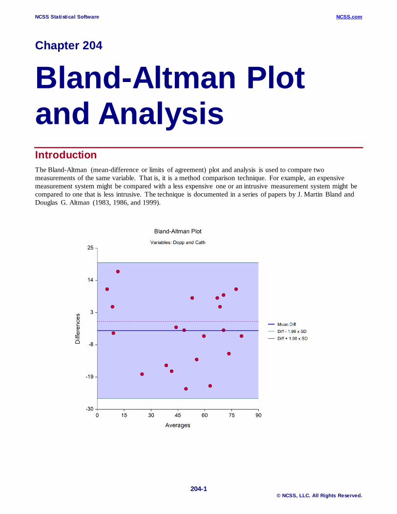
NCSS Statistical Software NCSS.com Bland-Altman Plot and Analysis


Repeatability An important part of method comparison is to understand how repeatable the measurement system is. This can only be understood by sampling each subject multiple times on the same method. This provides for the analysis of designs that include replicates.

Technical Details for Three Designs There are three study designs that can be analyzed by this procedure. Each type has different input and different technical details and the output is not identical. The technical details of each design will be presented here.

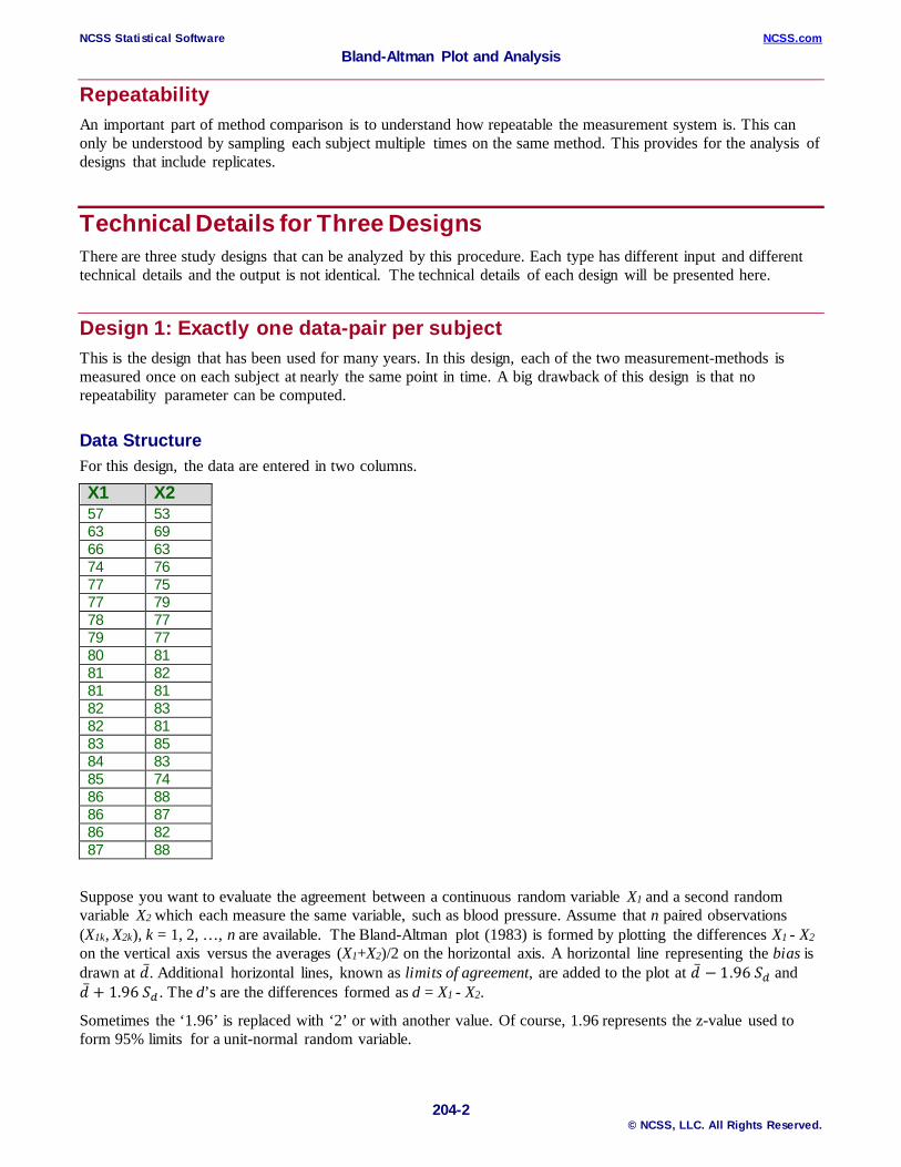
Design 1: Exactly one data-pair per subject This is the design that has been used for many years. In this design, each of the two measurement-methods is measured once on each subject at nearly the same point in time. A big drawback of this design is that no repeatability parameter can be computed.

Data Structure For this design, the data are entered in two columns.

X1 X2 57 53 63 69 66 63 74 76 77 75 77 79 78 77 79 77 80 81 81 82 81 81 82 83 82 81 83 85 84 83 85 74 86 88 86 87 86 82 87 88

Suppose you want to evaluate the agreement between a continuous random variable X1 and a second random variable X2 which each measure the same variable, such as blood pressure. Assume that n paired observations (X1k, X2k), k = 1, 2, …, n are available. The Bland-Altman plot (1983) is formed by plotting the differences X1 - X2 on the vertical axis versus the averages (X1+X2)/2 on the horizontal axis. A horizontal line representing the bias is drawn at �̅�𝑑. Additional horizontal lines, known as limits of agreement, are added to the plot at �̅�𝑑 − 1.96 𝑆𝑆𝑑𝑑 and �̅�𝑑 + 1.96 𝑆𝑆𝑑𝑑 . The d’s are the differences formed as d = X1 - X2.

Sometimes the ‘1.96’ is replaced with ‘2’ or with another value. Of course, 1.96 represents the z-value used to form 95% limits for a unit-normal random variable.




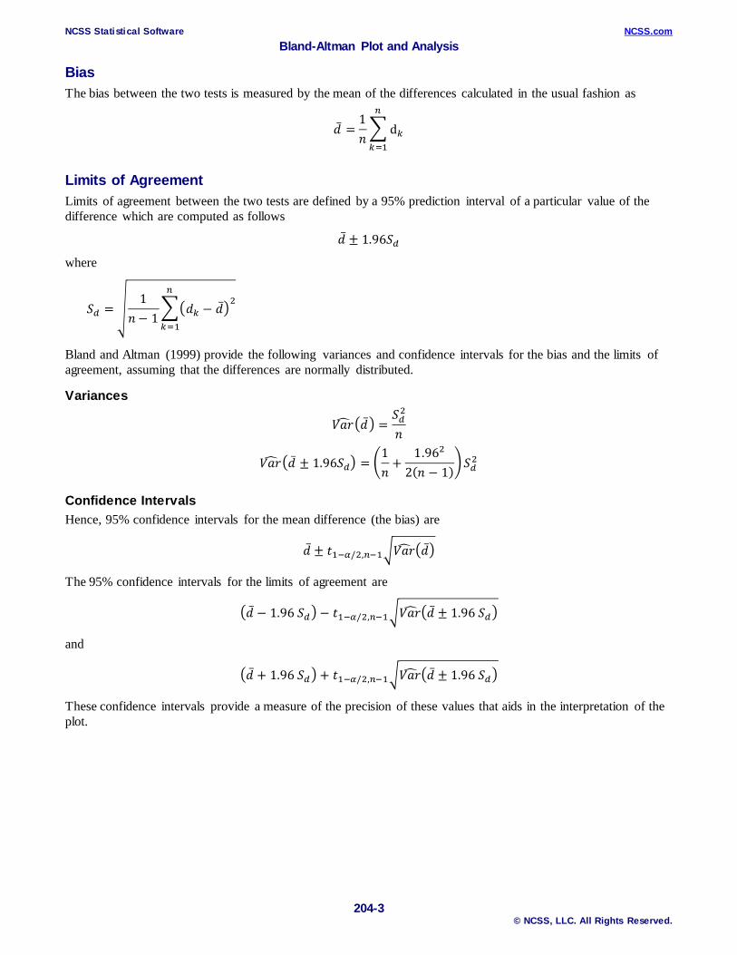
Bias The bias between the two tests is measured by the mean of the differences calculated in the usual fashion as

�̅�𝑑 =1𝑛𝑛� d𝑘𝑘

𝑛𝑛

𝑘𝑘=1

Limits of Agreement Limits of agreement between the two tests are defined by a 95% prediction interval of a particular value of the difference which are computed as follows

�̅�𝑑 ± 1.96𝑆𝑆𝑑𝑑

where

𝑆𝑆𝑑𝑑 = �1

𝑛𝑛 − 1��𝑑𝑑𝑘𝑘 − �̅�𝑑�

2𝑛𝑛

𝑘𝑘=1

Bland and Altman (1999) provide the following variances and confidence intervals for the bias and the limits of agreement, assuming that the differences are normally distributed.

Variances

𝑉𝑉𝑉𝑉𝑉𝑉� ��̅�𝑑� =𝑆𝑆𝑑𝑑2

𝑛𝑛

𝑉𝑉𝑉𝑉𝑉𝑉� ��̅�𝑑 ± 1.96𝑆𝑆𝑑𝑑� = �1𝑛𝑛

+1.962

2(𝑛𝑛 − 1)�𝑆𝑆𝑑𝑑2

Confidence Intervals Hence, 95% confidence intervals for the mean difference (the bias) are

�̅�𝑑 ± 𝑡𝑡1−𝛼𝛼/2,𝑛𝑛−1�𝑉𝑉𝑉𝑉𝑉𝑉� ��̅�𝑑�

The 95% confidence intervals for the limits of agreement are

��̅�𝑑 − 1.96 𝑆𝑆𝑑𝑑� − 𝑡𝑡1−𝛼𝛼/2,𝑛𝑛−1�𝑉𝑉𝑉𝑉𝑉𝑉� ��̅�𝑑 ± 1.96 𝑆𝑆𝑑𝑑�

and

��̅�𝑑 + 1.96 𝑆𝑆𝑑𝑑� + 𝑡𝑡1−𝛼𝛼/2,𝑛𝑛−1�𝑉𝑉𝑉𝑉𝑉𝑉� ��̅�𝑑 ± 1.96 𝑆𝑆𝑑𝑑�

These confidence intervals provide a measure of the precision of these values that aids in the interpretation of the plot.




Design 2: Multiple replicates for each method, no pairing In this Bland-Altman design, each subject is measured several times (usually in immediate succession) on one method and then measured several times on the other method. There is no natural pairing of the measures. In fact, the number of replicates does not have to be the same for each method. It is assumed that the overall response mean stays constant throughout the data gathering period.

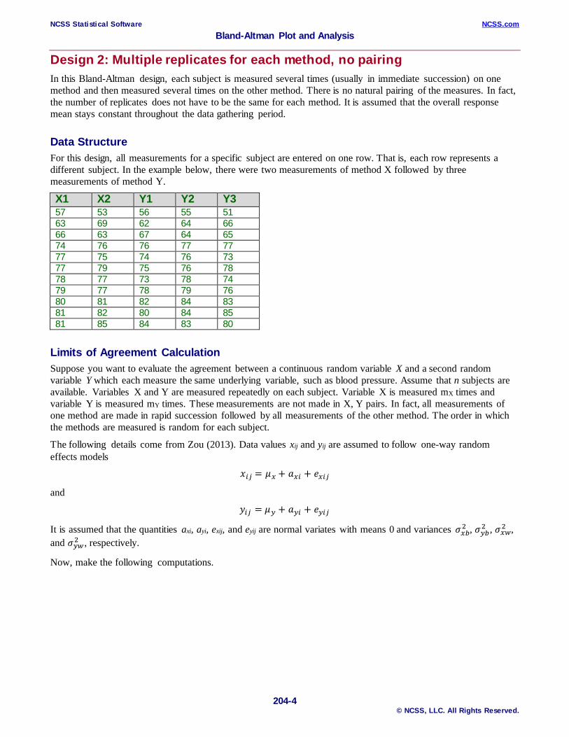
Data Structure For this design, all measurements for a specific subject are entered on one row. That is, each row represents a different subject. In the example below, there were two measurements of method X followed by three measurements of method Y.

X1 X2 Y1 Y2 Y3 57 53 56 55 51 63 69 62 64 66 66 63 67 64 65 74 76 76 77 77 77 75 74 76 73 77 79 75 76 78 78 77 73 78 74 79 77 78 79 76 80 81 82 84 83 81 82 80 84 85 81 85 84 83 80

Limits of Agreement Calculation Suppose you want to evaluate the agreement between a continuous random variable X and a second random variable Y which each measure the same underlying variable, such as blood pressure. Assume that n subjects are available. Variables X and Y are measured repeatedly on each subject. Variable X is measured mX times and variable Y is measured mY times. These measurements are not made in X, Y pairs. In fact, all measurements of one method are made in rapid succession followed by all measurements of the other method. The order in which the methods are measured is random for each subject.

The following details come from Zou (2013). Data values xij and yij are assumed to follow one-way random effects models

𝑥𝑥𝑖𝑖𝑖𝑖 = 𝜇𝜇𝑥𝑥 + 𝑉𝑉𝑥𝑥𝑖𝑖 + 𝑒𝑒𝑥𝑥𝑖𝑖𝑖𝑖

and

𝑦𝑦𝑖𝑖𝑖𝑖 = 𝜇𝜇𝑦𝑦 + 𝑉𝑉𝑦𝑦𝑖𝑖 + 𝑒𝑒𝑦𝑦𝑖𝑖𝑖𝑖

It is assumed that the quantities axi, ayi, exij, and eyij are normal variates with means 0 and variances 𝜎𝜎𝑥𝑥𝑥𝑥2 , 𝜎𝜎𝑦𝑦𝑥𝑥2 , 𝜎𝜎𝑥𝑥𝑥𝑥2 , and 𝜎𝜎𝑦𝑦𝑥𝑥2 , respectively.

Now, make the following computations.




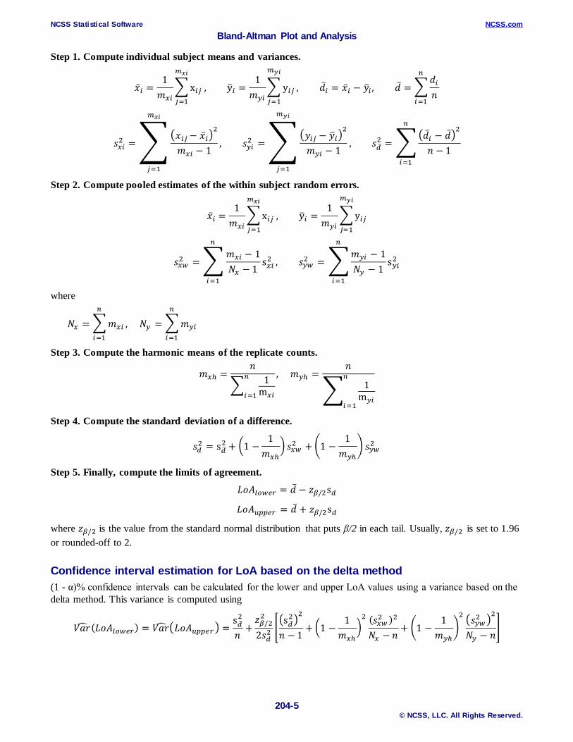
Step 1. Compute individual subject means and variances.

�̅�𝑥𝑖𝑖 =1𝑚𝑚𝑥𝑥𝑖𝑖

� x𝑖𝑖𝑖𝑖

𝑚𝑚𝑥𝑥𝑥𝑥

𝑖𝑖=1

, 𝑦𝑦�𝑖𝑖 =1𝑚𝑚𝑦𝑦𝑖𝑖

� y𝑖𝑖𝑖𝑖

𝑚𝑚𝑦𝑦𝑥𝑥

𝑖𝑖=1

, �̅�𝑑𝑖𝑖 = �̅�𝑥𝑖𝑖 − 𝑦𝑦�𝑖𝑖 , �̅�𝑑 = �𝑑𝑑𝑖𝑖𝑛𝑛

𝑛𝑛

𝑖𝑖=1

𝑠𝑠𝑥𝑥𝑖𝑖2 = ��𝑥𝑥𝑖𝑖𝑖𝑖 − �̅�𝑥𝑖𝑖�

2

𝑚𝑚𝑥𝑥𝑖𝑖 − 1


𝑖𝑖=1

, 𝑠𝑠𝑦𝑦𝑖𝑖2 = ��𝑦𝑦𝑖𝑖𝑖𝑖 − 𝑦𝑦�𝑖𝑖�

2

𝑚𝑚𝑦𝑦𝑖𝑖 − 1


𝑖𝑖=1

, 𝑠𝑠𝑑𝑑�2 = �

��̅�𝑑𝑖𝑖 − �̅�𝑑�2

𝑛𝑛 − 1

𝑛𝑛

𝑖𝑖=1

Step 2. Compute pooled estimates of the within subject random errors.

�̅�𝑥𝑖𝑖 =1𝑚𝑚𝑥𝑥𝑖𝑖

� x𝑖𝑖𝑖𝑖


𝑖𝑖=1

, 𝑦𝑦�𝑖𝑖 =1𝑚𝑚𝑦𝑦𝑖𝑖

� y𝑖𝑖𝑖𝑖


𝑖𝑖=1

𝑠𝑠𝑥𝑥𝑥𝑥2 = �𝑚𝑚𝑥𝑥𝑖𝑖 − 1𝑁𝑁𝑥𝑥 − 1

s𝑥𝑥𝑖𝑖2𝑛𝑛

𝑖𝑖=1

, 𝑠𝑠𝑦𝑦𝑥𝑥2 = �𝑚𝑚𝑦𝑦𝑖𝑖 − 1𝑁𝑁𝑦𝑦 − 1

s𝑦𝑦𝑖𝑖2𝑛𝑛

𝑖𝑖=1

where

𝑁𝑁𝑥𝑥 = �𝑚𝑚𝑥𝑥𝑖𝑖

𝑛𝑛

𝑖𝑖=1

, 𝑁𝑁𝑦𝑦 = �𝑚𝑚𝑦𝑦𝑖𝑖

𝑛𝑛

𝑖𝑖=1

Step 3. Compute the harmonic means of the replicate counts.

𝑚𝑚𝑥𝑥ℎ =𝑛𝑛

� 1m𝑥𝑥𝑖𝑖

𝑛𝑛

𝑖𝑖=1

, 𝑚𝑚𝑦𝑦ℎ =𝑛𝑛

� 1m𝑦𝑦𝑖𝑖

𝑛𝑛

𝑖𝑖=1

Step 4. Compute the standard deviation of a difference.

𝑠𝑠𝑑𝑑2 = s𝑑𝑑�2 + �1 −

1𝑚𝑚𝑥𝑥ℎ

� 𝑠𝑠𝑥𝑥𝑥𝑥2 + �1 −1𝑚𝑚𝑦𝑦ℎ

� 𝑠𝑠𝑦𝑦𝑥𝑥2

Step 5. Finally, compute the limits of agreement.

𝐿𝐿𝐿𝐿𝐿𝐿𝑙𝑙𝑙𝑙𝑥𝑥𝑙𝑙𝑙𝑙 = �̅�𝑑 − 𝑧𝑧𝛽𝛽/2s𝑑𝑑

𝐿𝐿𝐿𝐿𝐿𝐿𝑢𝑢𝑢𝑢𝑢𝑢𝑙𝑙𝑙𝑙 = �̅�𝑑 + 𝑧𝑧𝛽𝛽/2s𝑑𝑑

where 𝑧𝑧𝛽𝛽/2 is the value from the standard normal distribution that puts β/2 in each tail. Usually, 𝑧𝑧𝛽𝛽/2 is set to 1.96 or rounded-off to 2.

Confidence interval estimation for LoA based on the delta method (1 - α)% confidence intervals can be calculated for the lower and upper LoA values using a variance based on the delta method. This variance is computed using

𝑉𝑉𝑉𝑉𝑉𝑉� (𝐿𝐿𝐿𝐿𝐿𝐿𝑙𝑙𝑙𝑙𝑥𝑥𝑙𝑙𝑙𝑙) = 𝑉𝑉𝑉𝑉𝑉𝑉� �𝐿𝐿𝐿𝐿𝐿𝐿𝑢𝑢𝑢𝑢𝑢𝑢𝑙𝑙𝑙𝑙� =s𝑑𝑑�2

𝑛𝑛+𝑧𝑧𝛽𝛽/22

2𝑠𝑠𝑑𝑑2��s𝑑𝑑�

2�2

𝑛𝑛 − 1+ �1 −

1𝑚𝑚𝑥𝑥ℎ

�2 (𝑠𝑠𝑥𝑥𝑥𝑥2 )2

𝑁𝑁𝑥𝑥 − 𝑛𝑛+ �1 −

1𝑚𝑚𝑦𝑦ℎ

�2 �𝑠𝑠𝑦𝑦𝑥𝑥2 �2

𝑁𝑁𝑦𝑦 − 𝑛𝑛�




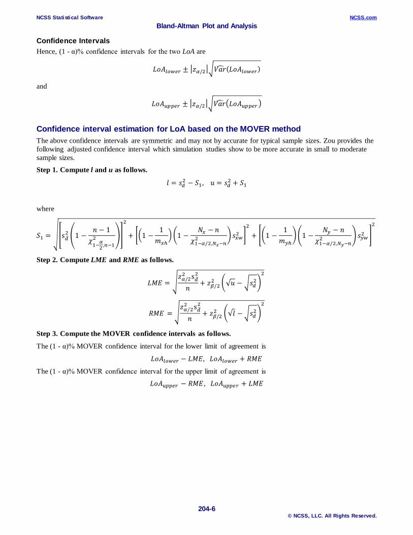
Confidence Intervals Hence, (1 - α)% confidence intervals for the two LoA are

𝐿𝐿𝐿𝐿𝐿𝐿𝑙𝑙𝑙𝑙𝑥𝑥𝑙𝑙𝑙𝑙 ± �𝑧𝑧𝛼𝛼/2��𝑉𝑉𝑉𝑉𝑉𝑉� (𝐿𝐿𝐿𝐿𝐿𝐿𝑙𝑙𝑙𝑙𝑥𝑥𝑙𝑙𝑙𝑙)

and

𝐿𝐿𝐿𝐿𝐿𝐿𝑢𝑢𝑢𝑢𝑢𝑢𝑙𝑙𝑙𝑙 ± �𝑧𝑧𝛼𝛼/2��𝑉𝑉𝑉𝑉𝑉𝑉� �𝐿𝐿𝐿𝐿𝐿𝐿𝑢𝑢𝑢𝑢𝑢𝑢𝑙𝑙𝑙𝑙�

Confidence interval estimation for LoA based on the MOVER method The above confidence intervals are symmetric and may not by accurate for typical sample sizes. Zou provides the following adjusted confidence interval which simulation studies show to be more accurate in small to moderate sample sizes.

Step 1. Compute l and u as follows.

𝑙𝑙 = 𝑠𝑠𝑑𝑑2 − 𝑆𝑆1 , 𝑢𝑢 = 𝑠𝑠𝑑𝑑2 + 𝑆𝑆1

where

𝑆𝑆1 = ��s𝑑𝑑�2 �1 −

𝑛𝑛 − 1𝜒𝜒1−𝛼𝛼2 ,𝑛𝑛−12 ��

2

+ ��1 −1𝑚𝑚𝑥𝑥ℎ

� �1 −𝑁𝑁𝑥𝑥 − 𝑛𝑛

𝜒𝜒1−𝛼𝛼/2,𝑁𝑁𝑥𝑥−𝑛𝑛2 � 𝑠𝑠𝑥𝑥𝑥𝑥2 �

2

+ ��1 −1𝑚𝑚𝑦𝑦ℎ

��1 −𝑁𝑁𝑦𝑦 − 𝑛𝑛

𝜒𝜒1−𝛼𝛼/2,𝑁𝑁𝑦𝑦−𝑛𝑛2 � 𝑠𝑠𝑦𝑦𝑥𝑥2 �

2

Step 2. Compute LME and RME as follows.

𝐿𝐿𝐿𝐿𝐿𝐿 = �𝑧𝑧𝛼𝛼/22 s𝑑𝑑�

2

𝑛𝑛+ 𝑧𝑧𝛽𝛽/2

2 �√𝑢𝑢 − �𝑠𝑠𝑑𝑑2�2

𝑅𝑅𝐿𝐿𝐿𝐿 = �𝑧𝑧𝛼𝛼/22 s𝑑𝑑�

2


2 �√𝑙𝑙 −�𝑠𝑠𝑑𝑑2�2

Step 3. Compute the MOVER confidence intervals as follows.

The (1 - α)% MOVER confidence interval for the lower limit of agreement is

𝐿𝐿𝐿𝐿𝐿𝐿𝑙𝑙𝑙𝑙𝑥𝑥𝑙𝑙𝑙𝑙 − 𝐿𝐿𝐿𝐿𝐿𝐿, 𝐿𝐿𝐿𝐿𝐿𝐿𝑙𝑙𝑙𝑙𝑥𝑥𝑙𝑙𝑙𝑙 + 𝑅𝑅𝐿𝐿𝐿𝐿

The (1 - α)% MOVER confidence interval for the upper limit of agreement is

𝐿𝐿𝐿𝐿𝐿𝐿𝑢𝑢𝑢𝑢𝑢𝑢𝑙𝑙𝑙𝑙 − 𝑅𝑅𝐿𝐿𝐿𝐿 , 𝐿𝐿𝐿𝐿𝐿𝐿𝑢𝑢𝑢𝑢𝑢𝑢𝑙𝑙𝑙𝑙 + 𝐿𝐿𝐿𝐿𝐿𝐿




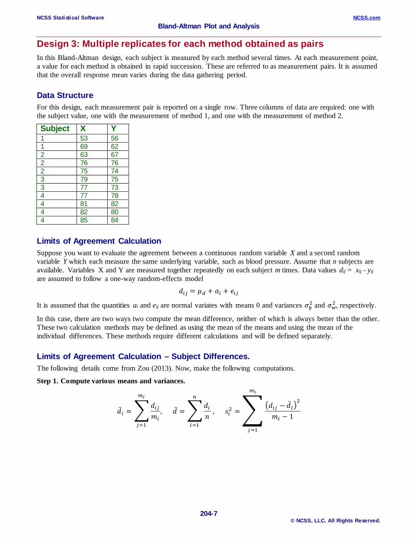
Design 3: Multiple replicates for each method obtained as pairs In this Bland-Altman design, each subject is measured by each method several times. At each measurement point, a value for each method is obtained in rapid succession. These are referred to as measurement pairs. It is assumed that the overall response mean varies during the data gathering period.

Data Structure For this design, each measurement pair is reported on a single row. Three columns of data are required: one with the subject value, one with the measurement of method 1, and one with the measurement of method 2.

Subject X Y 1 53 56 1 69 62 2 63 67 2 76 76 2 75 74 3 79 75 3 77 73 4 77 78 4 81 82 4 82 80 4 85 84

Limits of Agreement Calculation Suppose you want to evaluate the agreement between a continuous random variable X and a second random variable Y which each measure the same underlying variable, such as blood pressure. Assume that n subjects are available. Variables X and Y are measured together repeatedly on each subject m times. Data values dij = xij - yij are assumed to follow a one-way random-effects model

𝑑𝑑𝑖𝑖𝑖𝑖 = 𝜇𝜇𝑑𝑑 + 𝑉𝑉𝑖𝑖 + 𝑒𝑒𝑖𝑖𝑖𝑖

It is assumed that the quantities ai and eij are normal variates with means 0 and variances 𝜎𝜎𝑥𝑥2 and 𝜎𝜎𝑥𝑥2 , respectively.

In this case, there are two ways two compute the mean difference, neither of which is always better than the other. These two calculation methods may be defined as using the mean of the means and using the mean of the individual differences. These methods require different calculations and will be defined separately.

Limits of Agreement Calculation – Subject Differences. The following details come from Zou (2013). Now, make the following computations.

Step 1. Compute various means and variances.

�̅�𝑑𝑖𝑖 = �𝑑𝑑𝑖𝑖𝑖𝑖𝑚𝑚𝑖𝑖

𝑚𝑚𝑥𝑥

𝑖𝑖=1

, �̅�𝑑 = �𝑑𝑑𝑖𝑖𝑛𝑛

𝑛𝑛

𝑖𝑖=1

, 𝑠𝑠𝑖𝑖2 = ��𝑑𝑑𝑖𝑖𝑖𝑖 − �̅�𝑑𝑖𝑖�

2

𝑚𝑚𝑖𝑖 − 1

𝑚𝑚𝑥𝑥

𝑖𝑖=1




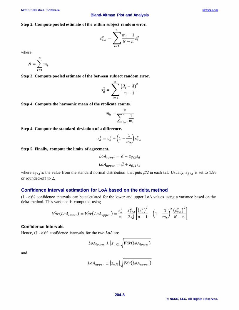
Step 2. Compute pooled estimate of the within subject random error.

𝑠𝑠𝑑𝑑𝑥𝑥2 = �𝑚𝑚𝑖𝑖 − 1𝑁𝑁 − 𝑛𝑛

𝑠𝑠𝑖𝑖2𝑛𝑛

𝑖𝑖=1

where

𝑁𝑁 = �𝑚𝑚𝑖𝑖

𝑛𝑛

𝑖𝑖=1

Step 3. Compute pooled estimate of the between subject random error.

𝑠𝑠𝑑𝑑�2 = �

��̅�𝑑𝑖𝑖 − �̅�𝑑�2

𝑛𝑛 − 1

𝑛𝑛

𝑖𝑖=1

Step 4. Compute the harmonic mean of the replicate counts.

𝑚𝑚ℎ =𝑛𝑛

� 1m𝑖𝑖

𝑛𝑛

𝑖𝑖=1

Step 4. Compute the standard deviation of a difference.

𝑠𝑠𝑑𝑑2 = s𝑑𝑑�2 + �1 −

1𝑚𝑚ℎ

� 𝑠𝑠𝑑𝑑𝑥𝑥2

Step 5. Finally, compute the limits of agreement.

𝐿𝐿𝐿𝐿𝐿𝐿𝑙𝑙𝑙𝑙𝑥𝑥𝑙𝑙𝑙𝑙 = �̅�𝑑 − 𝑧𝑧𝛽𝛽/2s𝑑𝑑

𝐿𝐿𝐿𝐿𝐿𝐿𝑢𝑢𝑢𝑢𝑢𝑢𝑙𝑙𝑙𝑙 = �̅�𝑑 + 𝑧𝑧𝛽𝛽/2s𝑑𝑑

where 𝑧𝑧𝛽𝛽/2 is the value from the standard normal distribution that puts β/2 in each tail. Usually, 𝑧𝑧𝛽𝛽/2 is set to 1.96 or rounded-off to 2.

Confidence interval estimation for LoA based on the delta method (1 - α)% confidence intervals can be calculated for the lower and upper LoA values using a variance based on the delta method. This variance is computed using

𝑉𝑉𝑉𝑉𝑉𝑉� (𝐿𝐿𝐿𝐿𝐿𝐿𝑙𝑙𝑙𝑙𝑥𝑥𝑙𝑙𝑙𝑙) = 𝑉𝑉𝑉𝑉𝑉𝑉� �𝐿𝐿𝐿𝐿𝐿𝐿𝑢𝑢𝑢𝑢𝑢𝑢𝑙𝑙𝑙𝑙 � =s𝑑𝑑�2

𝑛𝑛+𝑧𝑧𝛽𝛽/22

2𝑠𝑠𝑑𝑑2��s𝑑𝑑�

2�2

𝑛𝑛 − 1+ �1 −

1𝑚𝑚ℎ

�2 �𝑠𝑠𝑑𝑑𝑥𝑥2 �2

𝑁𝑁 − 𝑛𝑛�

Confidence Intervals Hence, (1 - α)% confidence intervals for the two LoA are

𝐿𝐿𝐿𝐿𝐿𝐿𝑙𝑙𝑙𝑙𝑥𝑥𝑙𝑙𝑙𝑙 ± �𝑧𝑧𝛼𝛼/2��𝑉𝑉𝑉𝑉𝑉𝑉� (𝐿𝐿𝐿𝐿𝐿𝐿𝑙𝑙𝑙𝑙𝑥𝑥𝑙𝑙𝑙𝑙)

and

𝐿𝐿𝐿𝐿𝐿𝐿𝑢𝑢𝑢𝑢𝑢𝑢𝑙𝑙𝑙𝑙 ± �𝑧𝑧𝛼𝛼/2��𝑉𝑉𝑉𝑉𝑉𝑉� �𝐿𝐿𝐿𝐿𝐿𝐿𝑢𝑢𝑢𝑢𝑢𝑢𝑙𝑙𝑙𝑙�




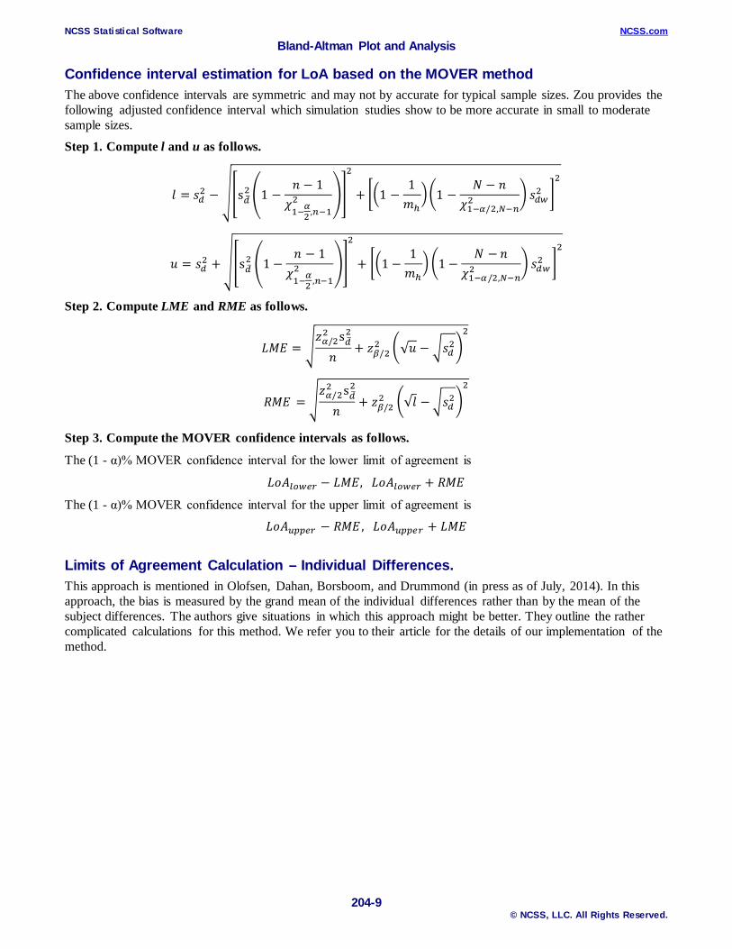
Confidence interval estimation for LoA based on the MOVER method The above confidence intervals are symmetric and may not by accurate for typical sample sizes. Zou provides the following adjusted confidence interval which simulation studies show to be more accurate in small to moderate sample sizes.

Step 1. Compute l and u as follows.

𝑙𝑙 = 𝑠𝑠𝑑𝑑2 − ��s𝑑𝑑�2 �1 −

𝑛𝑛 − 1𝜒𝜒1−𝛼𝛼2 ,𝑛𝑛−12 ��

2

+ ��1 −1𝑚𝑚ℎ

��1 −𝑁𝑁 − 𝑛𝑛

𝜒𝜒1−𝛼𝛼/2,𝑁𝑁−𝑛𝑛2 � 𝑠𝑠𝑑𝑑𝑥𝑥2 �

2

𝑢𝑢 = 𝑠𝑠𝑑𝑑2 +��s𝑑𝑑�2 �1 −

𝑛𝑛 − 1𝜒𝜒1−𝛼𝛼2 ,𝑛𝑛−12 ��

2

+ ��1 −1𝑚𝑚ℎ

� �1 −𝑁𝑁 −𝑛𝑛

𝜒𝜒1−𝛼𝛼/2,𝑁𝑁−𝑛𝑛2 � 𝑠𝑠𝑑𝑑𝑥𝑥2 �

2

Step 2. Compute LME and RME as follows.

𝐿𝐿𝐿𝐿𝐿𝐿 = �𝑧𝑧𝛼𝛼/22 s𝑑𝑑�

2


2 �√𝑢𝑢 − �𝑠𝑠𝑑𝑑2�2

𝑅𝑅𝐿𝐿𝐿𝐿 = �𝑧𝑧𝛼𝛼/22 s𝑑𝑑�

2


2 �√𝑙𝑙 −�𝑠𝑠𝑑𝑑2�2

Step 3. Compute the MOVER confidence intervals as follows.

The (1 - α)% MOVER confidence interval for the lower limit of agreement is

𝐿𝐿𝐿𝐿𝐿𝐿𝑙𝑙𝑙𝑙𝑥𝑥𝑙𝑙𝑙𝑙 − 𝐿𝐿𝐿𝐿𝐿𝐿, 𝐿𝐿𝐿𝐿𝐿𝐿𝑙𝑙𝑙𝑙𝑥𝑥𝑙𝑙𝑙𝑙 + 𝑅𝑅𝐿𝐿𝐿𝐿

The (1 - α)% MOVER confidence interval for the upper limit of agreement is

𝐿𝐿𝐿𝐿𝐿𝐿𝑢𝑢𝑢𝑢𝑢𝑢𝑙𝑙𝑙𝑙 − 𝑅𝑅𝐿𝐿𝐿𝐿 , 𝐿𝐿𝐿𝐿𝐿𝐿𝑢𝑢𝑢𝑢𝑢𝑢𝑙𝑙𝑙𝑙 + 𝐿𝐿𝐿𝐿𝐿𝐿

Limits of Agreement Calculation – Individual Differences. This approach is mentioned in Olofsen, Dahan, Borsboom, and Drummond (in press as of July, 2014). In this approach, the bias is measured by the grand mean of the individual differences rather than by the mean of the subject differences. The authors give situations in which this approach might be better. They outline the rather complicated calculations for this method. We refer you to their article for the details of our implementation of the method.




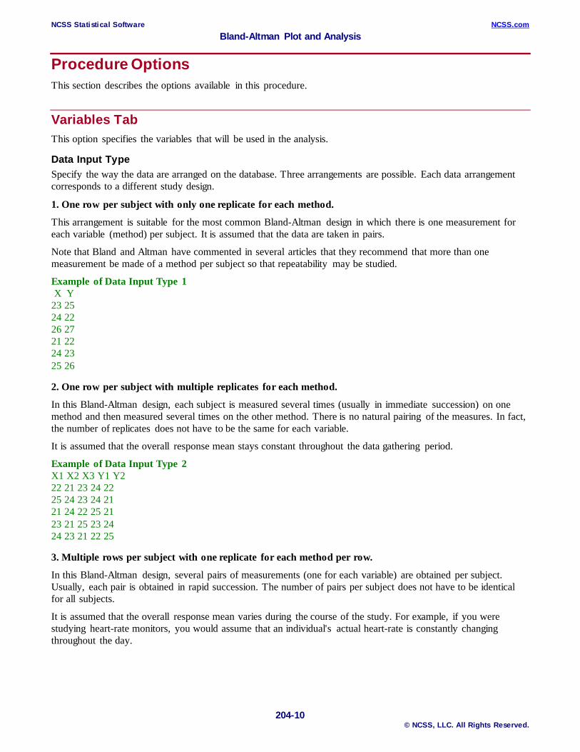
Procedure Options This section describes the options available in this procedure.

Variables Tab This option specifies the variables that will be used in the analysis.

Data Input Type Specify the way the data are arranged on the database. Three arrangements are possible. Each data arrangement corresponds to a different study design.

1. One row per subject with only one replicate for each method.

This arrangement is suitable for the most common Bland-Altman design in which there is one measurement for each variable (method) per subject. It is assumed that the data are taken in pairs.

Note that Bland and Altman have commented in several articles that they recommend that more than one measurement be made of a method per subject so that repeatability may be studied.

Example of Data Input Type 1 X Y 23 25 24 22 26 27 21 22 24 23 25 26 2. One row per subject with multiple replicates for each method.

In this Bland-Altman design, each subject is measured several times (usually in immediate succession) on one method and then measured several times on the other method. There is no natural pairing of the measures. In fact, the number of replicates does not have to be the same for each variable.

It is assumed that the overall response mean stays constant throughout the data gathering period.

Example of Data Input Type 2 X1 X2 X3 Y1 Y2 22 21 23 24 22 25 24 23 24 21 21 24 22 25 21 23 21 25 23 24 24 23 21 22 25 3. Multiple rows per subject with one replicate for each method per row.

In this Bland-Altman design, several pairs of measurements (one for each variable) are obtained per subject. Usually, each pair is obtained in rapid succession. The number of pairs per subject does not have to be identical for all subjects.

It is assumed that the overall response mean varies during the course of the study. For example, if you were studying heart-rate monitors, you would assume that an individual's actual heart-rate is constantly changing throughout the day.




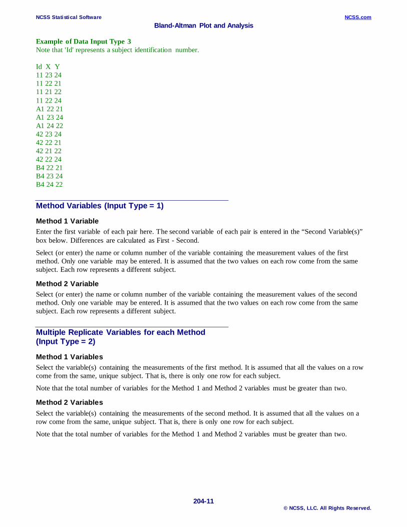
Example of Data Input Type 3 Note that 'Id' represents a subject identification number. Id X Y 11 23 24 11 22 21 11 21 22 11 22 24 A1 22 21 A1 23 24 A1 24 22 42 23 24 42 22 21 42 21 22 42 22 24 B4 22 21 B4 23 24 B4 24 22

Method Variables (Input Type = 1)

Method 1 Variable Enter the first variable of each pair here. The second variable of each pair is entered in the “Second Variable(s)” box below. Differences are calculated as First - Second.

Select (or enter) the name or column number of the variable containing the measurement values of the first method. Only one variable may be entered. It is assumed that the two values on each row come from the same subject. Each row represents a different subject.

Method 2 Variable Select (or enter) the name or column number of the variable containing the measurement values of the second method. Only one variable may be entered. It is assumed that the two values on each row come from the same subject. Each row represents a different subject.

Multiple Replicate Variables for each Method (Input Type = 2)

Method 1 Variables Select the variable(s) containing the measurements of the first method. It is assumed that all the values on a row come from the same, unique subject. That is, there is only one row for each subject.

Note that the total number of variables for the Method 1 and Method 2 variables must be greater than two.

Method 2 Variables Select the variable(s) containing the measurements of the second method. It is assumed that all the values on a row come from the same, unique subject. That is, there is only one row for each subject.

Note that the total number of variables for the Method 1 and Method 2 variables must be greater than two.




Subject Variable and Method Variables (Input Type = 3)

Subject Variable Specify (or enter) the name or column number of the variable containing the subject id values. These values may be text or numeric. These values are used to identify which rows are associated with which subjects.

Method 1 Variable Select (or enter) the name or column number of the variable containing the measurement values of the first method. Only one variable may be entered. It is assumed that the two values on each row come from the same subject. The database may contain several rows for each subject with one measurement pair per row.

Method 2 Variable Select (or enter) the name or column number of the variable containing the measurement values of the second method. Only one variable may be entered. It is assumed that the two values on each row come from the same subject. The database may contain several rows for each subject with one measurement pair per row.

Variables – Calculation Options These options specify which techniques and methods you want to use. Note that these options will only be displayed when they apply, depending on the setting of Data Input Type.

SD Multiplier for Limits of Agreement The limits of agreement are formed using the mean difference plus and minus the standard deviation of the difference times this multiplier value. Commonly, ‘1.96’ is used because, assuming a normal distribution, 95% of the data fall within these limits. Historically, this value was rounded to ‘2’ for convenience in computing the limits of agreement by hand.

Confidence Level of Confidence Intervals This confidence level is used for the confidence intervals of the means and agreement limits. Typical confidence levels are 90%, 95%, and 99%, with 95% being the most common.

Mean Difference (Bias) Estimation If each measurement method produced accurate measurements, the only difference between the means would be due to random error. Any systematic difference is called the bias.

There are two methods available for estimating the mean difference between the measurement methods.

• Subject Differences (Recommended) Compute the mean difference for each subject, then compute the mean of these mean differences.

• Individual Row Differences Calculate the mean difference for each row, then compute the mean of these means.

The most recommended method is the Subject Differences method. However, in some cases, the Individual Row Differences method may be better.

Note that this option only is available for Data Input Type 3. For Data Input Types 1 and 2, the Subject Differences method is used.




Limits of Agreement Confidence Interval There are two options available for computing a confidence interval for the limits of agreement (LoA): Delta Method and MOVER. This option specifies which of these methods to use.

• MOVER (Recommended) This method (Method Of Variance Estimates Recovery) has been shown by simulation studies to be more accurate than the delta method.

• Delta Method This is the classical method. This method produces symmetrical confidence limits. Simulation studies have shown this method to be inaccurate.

Reports Tab The options on this panel specify which reports will be included in the output.

Select Reports

Descriptive Statistics This section reports the count, mean, standard deviation, standard error, and mean for the specified variable.

Bland-Altman Analysis This provides a numeric report of the statistics used in the Bland-Altman plot.

Variance and Standard Deviation Reports This provides a numeric report of the statistics used in the Bland-Altman plot.

Test of Normality Assumption (Data Input Type = 1) This section reports a Shapiro-Wilk normality test.

Assumption Alpha This is the significance level of the Shapiro-Wilk normality test. A value of 0.05 is recommended. Typical values range from 0.001 to 0.200.

Report Options Tab The options on this panel control the label and decimal options of the report.

Report Options

Variable Names This option lets you select whether to display only variable names, variable labels, or both.




Decimal Places

Means, Differences, and Limits – Test Statistics These options specify the number of decimal places used in the reports. If one of the Auto options is used, the ending zero digits are not shown. For example, if ‘Significant Digits (Up to 7)’ is chosen, 0.0500 is displayed as 0.05 and 1.314583689 is displayed as 1.314584.

The output formatting system is not designed to accommodate (Up to 13), and if chosen, this will likely lead to lines that run on to a second line. This option is included, however, for the rare case when a very large number of decimals is needed.

Plots Tab The options on this panel control the inclusion and appearance of the plots. The plot format used depends on the setting of the Data Input Type setting

Select Plots

Bland-Altman Plot … Scatter Plot Check the boxes to display the plot. Click the plot format button to change the plot settings.




Example 1 – Bland-Altman Plots and Reports This section presents an example of how to generate a Bland-Altman plot. In this example, two measurements were made on each of 100 subjects. The first measurement was made by a lengthy, invasive method and the second measurement was made by a second, much less invasive method. The data are in the Bland-Altman dataset. The engineers wish to analyze whether the two methods agree.

You may follow along here by making the appropriate entries or load the completed template Example 1 by clicking on Open Example Template from the File menu of the Bland-Altman Plot window.

1 Open the Bland-Altman dataset. • From the File menu of the NCSS Data window, select Open Example Data. • Click on the file Bland-Altman.NCSS. • Click Open.

2 Open the Bland-Altman Plot window. • Using the Analysis or Graphics menu or the Procedure Navigator, find and select the Bland-Altman Plot

and Analysis procedure. • On the menus, select File, then New Template. This will fill the procedure with the default template.

3 Specify the variables. • Select the Variables tab. (This is the default.) • Set the Data Input Type to “1. One row per subject …” • Double-click in the Method 1 Variable box. This will bring up the variable selection window. • Select Method1 from the list of variables and then click Ok. “Method1” will appear in this box. • Double-click in the Method 2 Variable box. This will bring up the variable selection window. • Select Method2 from the list of variables and then click Ok. “Method2” will appear this box.

4 Run the procedure. • From the Run menu, select Run Procedure. Alternatively, just click the green Run button.

The following reports and charts will be displayed in the Output window.




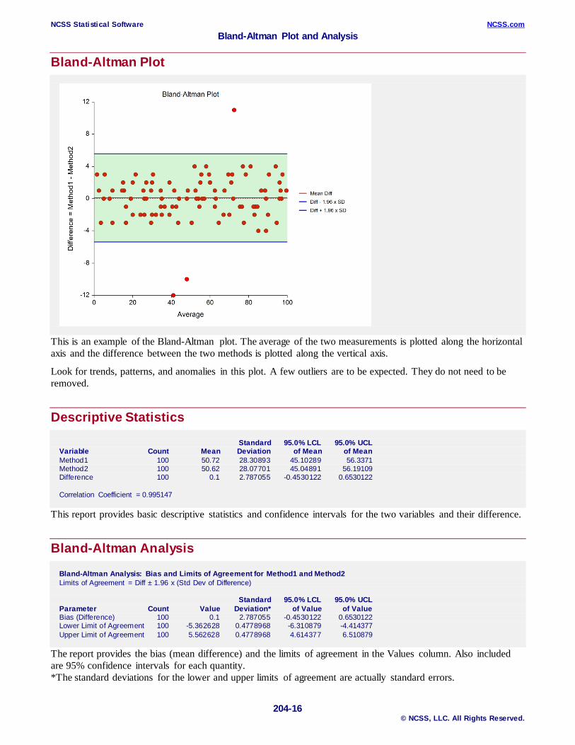
Bland-Altman Plot

This is an example of the Bland-Altman plot. The average of the two measurements is plotted along the horizontal axis and the difference between the two methods is plotted along the vertical axis.

Look for trends, patterns, and anomalies in this plot. A few outliers are to be expected. They do not need to be removed.

Descriptive Statistics Standard 95.0% LCL 95.0% UCL Variable Count Mean Deviation of Mean of Mean Method1 100 50.72 28.30893 45.10289 56.3371 Method2 100 50.62 28.07701 45.04891 56.19109 Difference 100 0.1 2.787055 -0.4530122 0.6530122 Correlation Coefficient = 0.995147 This report provides basic descriptive statistics and confidence intervals for the two variables and their difference.

Bland-Altman Analysis Bland-Altman Analysis: Bias and Limits of Agreement for Method1 and Method2 Limits of Agreement = Diff ± 1.96 x (Std Dev of Difference) Standard 95.0% LCL 95.0% UCL Parameter Count Value Deviation* of Value of Value Bias (Difference) 100 0.1 2.787055 -0.4530122 0.6530122 Lower Limit of Agreement 100 -5.362628 0.4778968 -6.310879 -4.414377 Upper Limit of Agreement 100 5.562628 0.4778968 4.614377 6.510879 The report provides the bias (mean difference) and the limits of agreement in the Values column. Also included are 95% confidence intervals for each quantity. *The standard deviations for the lower and upper limits of agreement are actually standard errors.




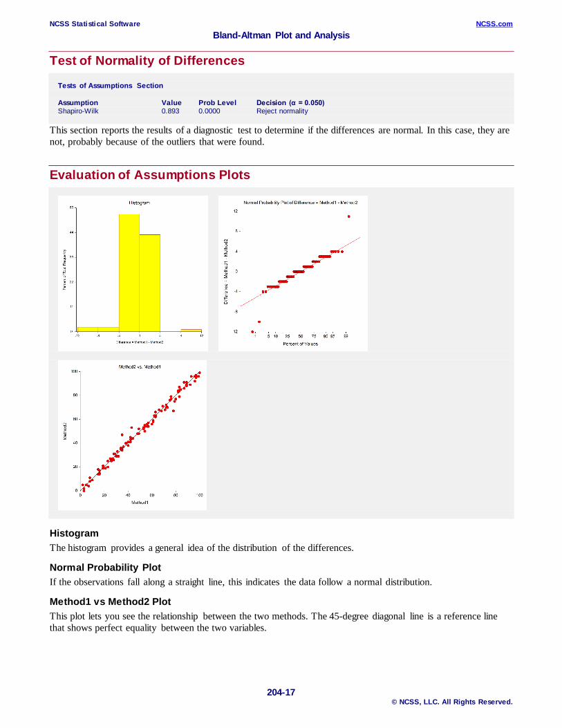
Test of Normality of Differences Tests of Assumptions Section Assumption Value Prob Level Decision (α = 0.050) Shapiro-Wilk 0.893 0.0000 Reject normality This section reports the results of a diagnostic test to determine if the differences are normal. In this case, they are not, probably because of the outliers that were found.

Evaluation of Assumptions Plots

Histogram The histogram provides a general idea of the distribution of the differences.

Normal Probability Plot If the observations fall along a straight line, this indicates the data follow a normal distribution.

Method1 vs Method2 Plot This plot lets you see the relationship between the two methods. The 45-degree diagonal line is a reference line that shows perfect equality between the two variables.




Example 2 – Bland-Altman Plot with Confidence Intervals This section shows the result of embellishing the standard Bland-Altman plot with confidence intervals for the three horizontal lines. The data are in the Bland-Altman dataset. You may follow along here by making the appropriate entries or load the completed template Example 2 by clicking on Open Example Template from the File menu of the Bland-Altman Plot window.

1 Open the Bland-Altman dataset. • From the File menu of the NCSS Data window, select Open Example Data. • Click on the file Bland-Altman.NCSS. • Click Open.



3 Specify the variables. • Select the Variables tab. (This is the default.) • Set the Data Input Type to “1. One row per subject …” • Double-click in the Method 1 Variable box. This will bring up the variable selection window. • Select Method1 from the list of variables and then click Ok. “Method1” will appear this box. • Double-click in the Method 2 Variable box. This will bring up the variable selection window. • Select Method2 from the list of variables and then click Ok. “Method2” will appear in this box.

4 Change the Plot Options. • Select the Plots tab. • Click the Bland-Altman Plot button. This will bring up the Bland-Altman Plot Format window. • Check the Fill box next to Mean Difference row. • Check the Fill box on the Lower Limit row. • Check the Fill box on the Upper Limit row.






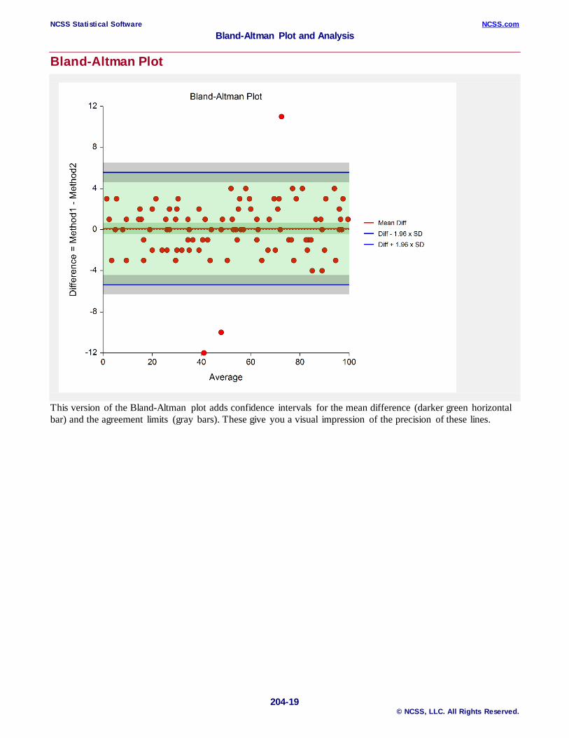
Bland-Altman Plot

This version of the Bland-Altman plot adds confidence intervals for the mean difference (darker green horizontal bar) and the agreement limits (gray bars). These give you a visual impression of the precision of these lines.




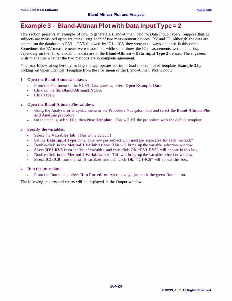
Example 3 – Bland-Altman Plot with Data Input Type = 2 This section presents an example of how to generate a Bland-Altman plot for Data Input Type 2. Suppose that 12 subjects are measured up to six times using each of two measurement devices: RV and IC. Although the data are entered on the database as RV1 – RV6 followed by IC1 – IC6, they were not always obtained in this order. Sometimes the RV measurements were made first, while other times the IC measurements were made first, depending on the flip of a coin. The data are in the Bland-Altman – Data Input Type 2 dataset. The engineers wish to analyze whether the two methods are in complete agreement.


1 Open the Bland-Altman2 dataset. • From the File menu of the NCSS Data window, select Open Example Data. • Click on the file Bland-Altman2.NCSS. • Click Open.



3 Specify the variables. • Select the Variables tab. (This is the default.) • Set the Data Input Type to “2. One row per subject with multiple replicates for each method.” • Double-click in the Method 1 Variables box. This will bring up the variable selection window. • Select RV1-RV6 from the list of variables and then click Ok. “RV1-RV6” will appear in this box. • Double-click in the Method 2 Variables box. This will bring up the variable selection window. • Select IC1-IC6 from the list of variables and then click Ok. “IC1-IC6” will appear this box.






Bland-Altman Plot

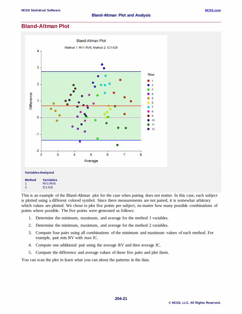
Variables Analyzed Method Variables 1 RV1-RV6 2 IC1-IC6 This is an example of the Bland-Altman plot for the case when pairing does not matter. In this case, each subject is plotted using a different colored symbol. Since there measurements are not paired, it is somewhat arbitrary which values are plotted. We chose to plot five points per subject, no matter how many possible combinations of points where possible. The five points were generated as follows:

1. Determine the minimum, maximum, and average for the method 1 variables.

2. Determine the minimum, maximum, and average for the method 2 variables.

3. Compute four pairs using all combinations of the minimum and maximum values of each method. For example, pair min RV with max IC.

4. Compute one additional pair using the average RV and then average IC.

5. Compute the difference and average values of these five pairs and plot them.

You can scan the plot to learn what you can about the patterns in the data.




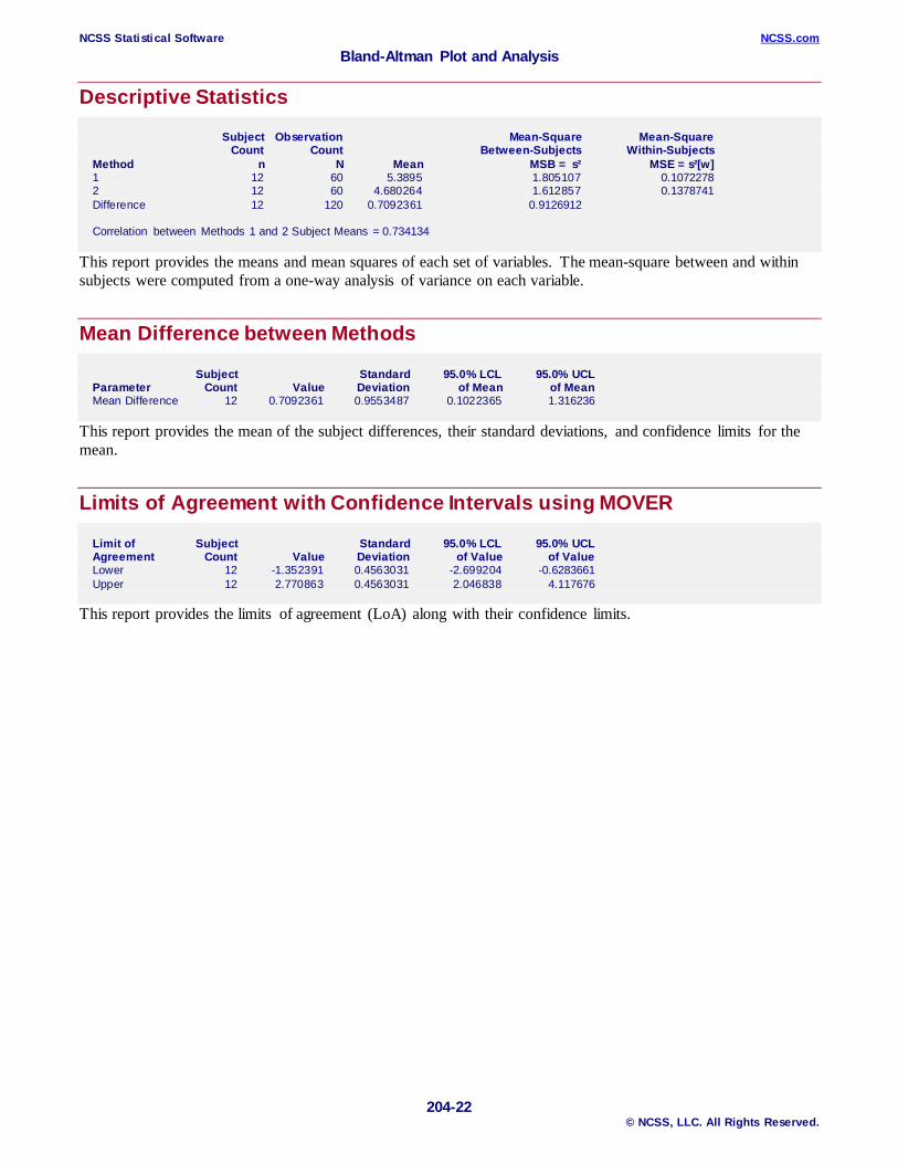
Descriptive Statistics Subject Observation Mean-Square Mean-Square Count Count Between-Subjects Within-Subjects Method n N Mean MSB = s² MSE = s²[w] 1 12 60 5.3895 1.805107 0.1072278 2 12 60 4.680264 1.612857 0.1378741 Difference 12 120 0.7092361 0.9126912 Correlation between Methods 1 and 2 Subject Means = 0.734134 This report provides the means and mean squares of each set of variables. The mean-square between and within subjects were computed from a one-way analysis of variance on each variable.

Mean Difference between Methods Subject Standard 95.0% LCL 95.0% UCL Parameter Count Value Deviation of Mean of Mean Mean Difference 12 0.7092361 0.9553487 0.1022365 1.316236 This report provides the mean of the subject differences, their standard deviations, and confidence limits for the mean.

Limits of Agreement with Confidence Intervals using MOVER Limit of Subject Standard 95.0% LCL 95.0% UCL Agreement Count Value Deviation of Value of Value Lower 12 -1.352391 0.4563031 -2.699204 -0.6283661 Upper 12 2.770863 0.4563031 2.046838 4.117676 This report provides the limits of agreement (LoA) along with their confidence limits.




Example 4 – Bland-Altman Plot with Data Input Type = 3 This section presents an example of how to generate a Bland-Altman plot for Data Input Type 3. Suppose that 12 subjects are measured a variable number of times on each of two measurement devices: RV and IC. Each measurement pair is recorded on a row of the database. The data are in the Bland-Altman – Data Input Type 3 dataset. The engineers wish to analyze whether the two methods are in complete agreement.


1 Open the Bland-Altman3 dataset. • From the File menu of the NCSS Data window, select Open Example Data. • Click on the file Bland-Altman3.NCSS. • Click Open.

2 Open the Bland-Altman Plot window. • Using the Analysis (or Graphics) menu or the Procedure Navigator, find and select the Bland-Altman

Plot procedure. • On the menus, select File, then New Template. This will fill the procedure with the default template.

3 Specify the variables. • Select the Variables tab. (This is the default.) • Set the Data Input Type to “3. Multiple rows per subject...” • Double-click in the Subject Variable box. This will bring up the variable selection window. • Select Subject from the list of variables and then click Ok. “Subject” will appear in this box. • Double-click in the Method 1 Variable box. This will bring up the variable selection window. • Select RV from the list of variables and then click Ok. “RV” will appear in this box. • Double-click in the Method 2 Variable box. This will bring up the variable selection window. • Select IC from the list of variables and then click Ok. “IC” will appear this box.






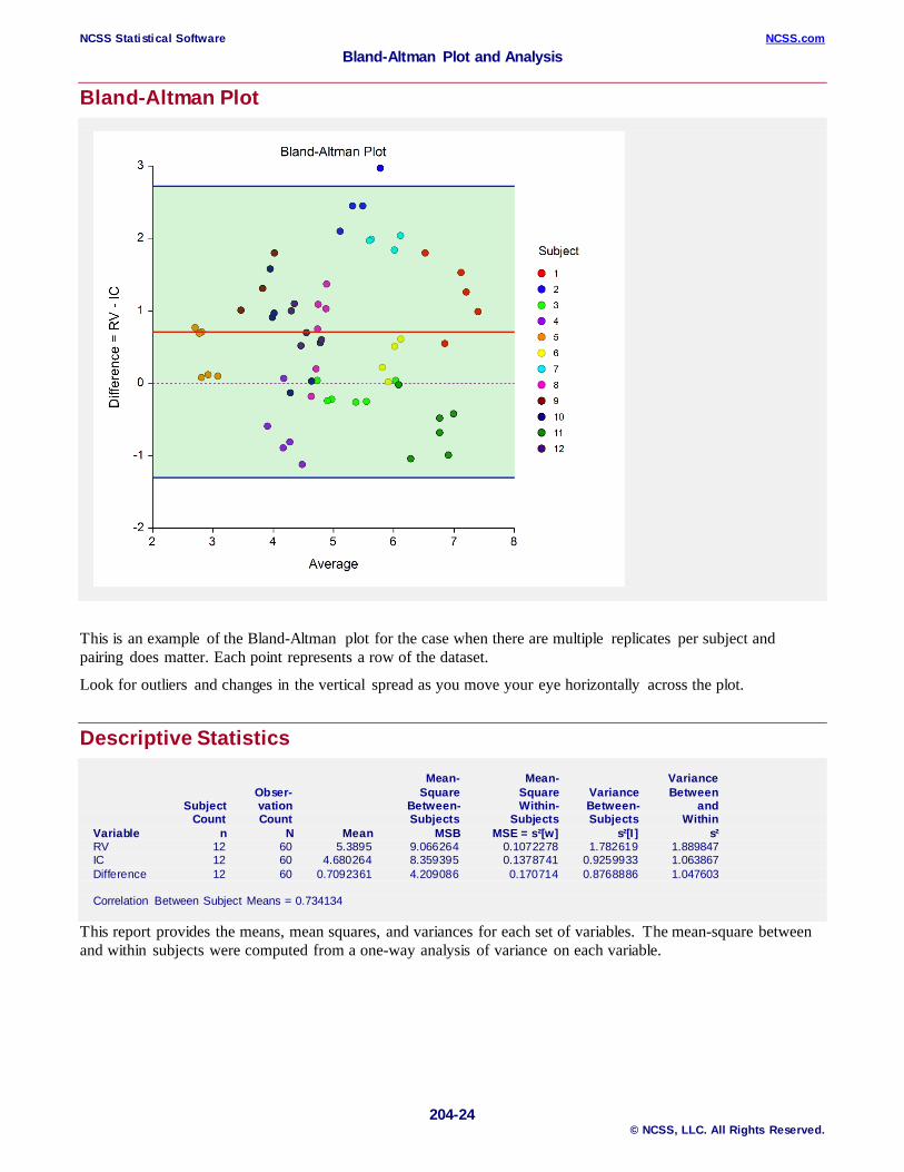
Bland-Altman Plot

This is an example of the Bland-Altman plot for the case when there are multiple replicates per subject and pairing does matter. Each point represents a row of the dataset.

Look for outliers and changes in the vertical spread as you move your eye horizontally across the plot.

Descriptive Statistics Mean- Mean- Variance Obser- Square Square Variance Between Subject vation Between- Within- Between- and Count Count Subjects Subjects Subjects Within Variable n N Mean MSB MSE = s²[w] s²[I ] s² RV 12 60 5.3895 9.066264 0.1072278 1.782619 1.889847 IC 12 60 4.680264 8.359395 0.1378741 0.9259933 1.063867 Difference 12 60 0.7092361 4.209086 0.170714 0.8768886 1.047603 Correlation Between Subject Means = 0.734134 This report provides the means, mean squares, and variances for each set of variables. The mean-square between and within subjects were computed from a one-way analysis of variance on each variable.




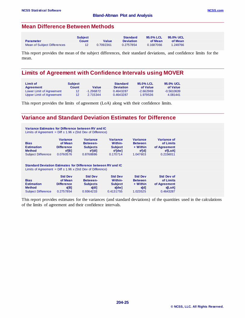
Mean Difference Between Methods Subject Standard 95.0% LCL 95.0% UCL Parameter Count Value Deviation of Mean of Mean Mean of Subject Differences 12 0.7092361 0.2757854 0.1687066 1.249766 This report provides the mean of the subject differences, their standard deviations, and confidence limits for the mean.

Limits of Agreement with Confidence Intervals using MOVER Limit of Subject Standard 95.0% LCL 95.0% UCL Agreement Count Value Deviation of Value of Value Lower Limit of Agreement 12 -1.296872 0.4643287 -2.662969 -0.5610639 Upper Limit of Agreement 12 2.715344 0.4643287 1.979536 4.081441 This report provides the limits of agreement (LoA) along with their confidence limits.

Variance and Standard Deviation Estimates for Difference Variance Estimates for Difference between RV and IC Limits of Agreement = Diff ± 1.96 x (Std Dev of Difference) Variance Variance Variance Variance Variance of Bias of Mean Between- Within- Between of Limits Estimation Difference Subjects Subject + Within of Agreement Method s²[B] s²[dI] s²[dw] s²[d] s²[LoA] Subject Difference 0.0760576 0.8768886 0.170714 1.047603 0.2156011 Standard Deviation Estimates for Difference between RV and IC Limits of Agreement = Diff ± 1.96 x (Std Dev of Difference) Std Dev Std Dev Std Dev Std Dev Std Dev of Bias of Mean Between- Within- Between of Limits Estimation Difference Subjects Subject + Within of Agreement Method s[B] s[dI] s[dw] s[d] s[LoA] Subject Difference 0.2757854 0.9364233 0.4131755 1.023525 0.4643287 This report provides estimates for the variances (and standard deviations) of the quantities used in the calculations of the limits of agreement and their confidence intervals.


Bland-Altman Plot and Analysis - Statistical Software · Bland-Altman Plot and Analysis...

Documents

Transcript of Bland-Altman Plot and Analysis - Statistical Software · Bland-Altman Plot and Analysis...